Vulnerability Assessment for Groundwater Dependent...

i

Depar tm ent o f Ea r t h Sc iences S im on F raser Un ive rs i t y

Mary Ann Middleton (Ph.D) and Diana M. Allen (Ph.D)

Department of Earth Sciences, Simon Fraser University

April 2016

Vulnerability Assessment for Groundwater Dependent Streams A guidance document describing a three level assessment approach for assessing the vulnerability of groundwater dependent streams to pumping.

ii

Table of Contents

1 Introduction ............................................................................................................................. 1

2 Background .............................................................................................................................. 2

2.1 Aquifer – Stream Connectivity ........................................................................................ 2

2.2 Assessing Connectivity .................................................................................................... 4

2.3 Aquifer – Stream System Types ....................................................................................... 5

2.4 Stressors and Stream Vulnerability ................................................................................. 7

3 Vulnerability Assessment for Groundwater Dependent Streams: Overview ........................ 11

3.1 Level I Assessment ......................................................................................................... 12

3.2 Level II Assessment ........................................................................................................ 12

3.3 Level III Assessment ....................................................................................................... 12

4 Level I Assessment: Potential Stream Vulnerability .............................................................. 12

4.1 Step 1: The Hydrologic Setting ...................................................................................... 13

4.1.1 Other Considerations ............................................................................................ 15

4.2 Step 2: Potential Stream Vulnerability .......................................................................... 16

4.2.1 Aquifer Productivity ............................................................................................... 16

Low (1) ........................................................................................................................................... 17

Moderate (2) ................................................................................................................................. 17

High (3) .......................................................................................................................................... 17

4.2.2 Groundwater Demand ........................................................................................... 17

4.2.3 Potential Stream Vulnerability .............................................................................. 18


4.2.5 Final Level I Assessment Criteria ........................................................................... 20

5 Level II Assessment: Rating Stream Vulnerability ................................................................. 21

5.1 Overview ........................................................................................................................ 21

5.2 Stream Susceptibility (SS) .............................................................................................. 21

5.2.1 Aquifer Characteristics (A) ..................................................................................... 22

5.2.2 Recharge to Stream (QR) ........................................................................................ 25

5.2.3 Summer Streamflow (QS) ....................................................................................... 27

5.2.4 Recharge Ratio (QS/QR) .......................................................................................... 27


iii

5.2.6 Stream Susceptibility (SS) Rating ........................................................................... 29

5.3 Hazard (H) ...................................................................................................................... 30


5.3.2 Hazard (H) Rating ................................................................................................... 31

5.4 Final Level II Assessment for Stream Vulnerability (SV) ................................................ 31

5.4.1 Example Level II Assessment ................................................................................. 32


6 Level III Assessment - Stream Impact .................................................................................... 37

6.1 Well Scale: Well Capture Zone Analysis ........................................................................ 37

6.2 Aquifer Scale Case Study ............................................................................................... 41

6.2.1 The Numerical Groundwater Flow Model ............................................................. 42

6.2.2 Comparing Annual Recharge and Baseflow under Non-Pumping Conditions ...... 45

6.2.3 Annual Recharge .................................................................................................... 45

6.2.4 Baseflow ................................................................................................................ 46

6.2.5 Comparing Pumping Impacts to the Stream Zones ............................................... 47

6.2.6 Comparing Impacts for Non-Pumping and Pumping ............................................. 50

6.2.7 Regional Monitoring: Field Indicators ................................................................... 50

6.2.8 Comparing Regional Field Measurements to Vulnerability Assessment Results .. 56


7 Risk Assessment / Risk Management Framework ................................................................. 57

7.1 Risk to a Stream ............................................................................................................. 58

7.2 Risk Management Example ........................................................................................... 58

8 References ............................................................................................................................. 60

Appendix A. Level III Assessment - Comparing Impacts for Non-Pumping and Pumping for Fishtrap and Bertrand Creek Watersheds ........................................................................... 67

Non-Pumping Impacts to the Watershed Zones ....................................................................... 67

Pumping Impacts to the Watershed Zones ............................................................................... 68

1

1 Introduction

This guidance document “Vulnerability Assessment for Groundwater Dependent Streams” (hereafter Stream Vulnerability Assessment), describes a multi-step, risk-based approach for evaluating the vulnerability of groundwater dependent streams to changes in the aquifer system. There is a particular emphasis on the summer low flow period, because it is during this time that streams can be sensitive to changes in the aquifer system; however, in principle the methodology can be used to assess stream vulnerability year round.

Understanding the likely response of streams to changes in the groundwater levels is important for integrated management of water quantity, quantity particularly in relation to groundwater pumping and its impact on stream flow. In many streams in the province of British Columbia (BC), stream flow during the annual summer low flow period1 is sustained by groundwater inputs (baseflow); as a result, such “groundwater dependent streams” can be sensitive to lower groundwater fluxes during this period. Streams with greater connectivity to the aquifer system2 may respond to changes in groundwater levels and fluxes, especially during the summer low flow period (Allen et al. 2010). Decreases in the timing and amount of precipitation as a result of climate change are projected for many areas of the province, and this has the potential to lead directly or indirectly to more extreme summer low flow events, and to extend the length of the summer low flow period in many streams (Déry et al. 2009). Climate variability and climate change have the potential to impact recharge conditions (e.g. Allen et al. 2004) as well as lead to increased water resource demands (e.g. Cohen et al. 2004), which in turn will lead to changes in groundwater conditions. Changes in land use/land cover (urbanization, timber harvesting, etc.) also impact recharge (Arnell 2002).

This guidance document also discusses how the Stream Vulnerability Assessment can be incorporated into a Risk Assessment / Risk Management Framework, to include indicators relevant to groundwater dependent streams and how these indicators may be used to inform decision making. The Vulnerability Assessment is envisioned to provide critical information for the Sensitive Stream Designation in BC. Under the Fish

1 In British Columbia, many streams also have a winter low flow period during which the streams may also be sensitive to changes in groundwater flux; however, this document is focused only on the summer period. 2 The “aquifer system” includes aquifers and aquitards, although the connection with a stream will be primarily through the more permeable geological units which are characterized as aquifers.

2

Protection Act, (Bill 25: FPA, 1997: Section 6(2)) a stream is designated a “sensitive stream” when it “contributes to the population of fish whose sustainability is at risk because of inadequate flow of water within the stream or degradation of fish habitat.” Under this regulation, a stream designated as sensitive will have mitigation measures and recovery plans in place to ensure sufficient water quantity for fish survival. The Sensitive Stream Designation is addressed in the Fish Protection Act (Bill 25: FPA, 1997) The Water Sustainability Act also addresses surface water and groundwater use including provision for environmental flows (Bill 18: WSA, 2014). The vulnerability assessment method presented in this document aims to contribute to the definition of a sensitive stream by including groundwater sensitive streams. A groundwater sensitive stream is herein defined as “a stream that is groundwater dependent and vulnerable to changes in the aquifer system, and is likely to have measurable impacts in water quantity to potential stressors.”

2 Background

2.1 Aquifer – Stream Connectivity

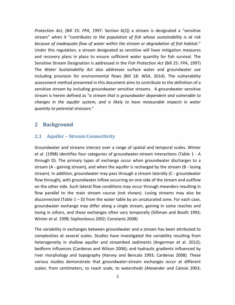
Groundwater and streams interact over a range of spatial and temporal scales. Winter et al. (1998) identifies four categories of groundwater-stream interactions (Table 1 - A through D). The primary types of exchange occur when groundwater discharges to a stream (A - gaining stream), and when the aquifer is recharged by the stream (B - losing stream). In addition, groundwater may pass through a stream laterally (C - groundwater flow through), with groundwater inflow occurring on one side of the stream and outflow on the other side. Such lateral flow conditions may occur through meanders resulting in flow parallel to the main stream course (not shown). Losing streams may also be disconnected (Table 1 – D) from the water table by an unsaturated zone. For each case, groundwater exchange may differ along a single stream, gaining in some reaches and losing in others, and these exchanges often vary temporally (Silliman and Booth 1993; Winter et al. 1998; Sophocleous 2002; Constantz 2008)

The variability in exchanges between groundwater and a stream has been attributed to complexities at several scales. Studies have investigated the variability resulting from heterogeneity in shallow aquifer and streambed sediments (Angerman et al. 2012); bedform influences (Cardenas and Wilson 2006); and hydraulic gradients influenced by river morphology and topography (Harvey and Bencala 1993; Cardenas 2008). These various studies demonstrate that groundwater-stream exchanges occur at different scales: from centimeters, to reach scale, to watersheds (Alexander and Caissie 2003;

3

Conant 2004, Anderson 2005; Constantz 2008). However, due to the complexities in the groundwater-stream exchanges, it can be challenging to extend field-based data (generally collected at the reach scale or smaller) into broader understanding of the processes driving the groundwater-surface water interactions at a watershed scale.

Table 1. Types of groundwater-stream interactions (adapted from Winter et al. 1998).

A - Gaining stream: Groundwater discharges into the stream. The water table in the vicinity of the stream is higher than the water level in the stream.

B - Losing stream: Stream water recharges the aquifer. The water table in the vicinity of the stream is lower than the water level in the stream.

C - Groundwater flow through: The groundwater flow direction is approx. perpendicular to the stream (or segment) and groundwater flows into one side of the stream, and outflows on the other side. The water table is higher on the upgradient side of the stream.

D - Disconnected stream: The water table is disconnected from the losing stream by an unsaturated zone. The water table is below the water level in the stream; however, localized mounding of the water table may occur in the vicinity of the stream.

4

2.2 Assessing Connectivity

Methods used to evaluate the connectivity between the aquifer and the stream are varied, and range from field-based methods to integrative approaches. The field based methods include direct methods for measuring exchanges between groundwater and surface water; indirect methods; and combinations of both (Cey et al. 1998; Essaid et al. 2008; Rosenberry and LaBaugh 2008). Direct methods include seepage meters, piezometers, and stream flow measurements (Boulton 1993; Baxter et al. 2003; Kalbus et al. 2006; Rosenberry 2008). Indirect methods include indicators such as water chemistry and mixing properties, or tracers such as heat (Stonestrom and Constantz 2003; Anderson 2005; Malcolm et al. 2005; Constantz 2008). The combination of methods can range from first-order assessments of the aquifer-stream system using mapping tools, to analytical solutions, to numerical modelling solutions.

Field measurements and integrative methods represent a spectrum of evaluation methods for groundwater-stream connectivity investigations. The integrative methods, such as numerical modelling, incorporate the field data, where available. Many studies have emphasized the benefits of using multiple methods to better quantify groundwater-stream interactions (Cey et al. 1998; Becker et al. 2004; Conant 2004; Kalbus et al. 2006; Brodie et al. 2009). Groundwater-stream exchanges often occur over a range of scales and in heterogeneous conditions; therefore, using a combination of methods is advantageous for understanding interactions in complex environments. A combination of methods reduces uncertainty, which may arise from limitations of the methods themselves, as well as errors and uncertainty in the available data. Use of multiple methods aids in linking information about the groundwater and the stream, and these linkages are necessary for assessment of connectivity. Lack of long term records for groundwater and streams can impede assessments of connectivity, and therefore the use of proxies, such as water temperature, can be incorporated within the spectrum of investigative methods.

Temperature is considered a robust and easily measured parameter for heat tracing and assessing groundwater interactions with streams (Anderson 2005; Caissie 2006; Hatch et al. 2006; Brewer 2013; Rau et al. 2014). At depths several metres below land surface, at which there is practically no annual fluctuation in ground temperature, groundwater temperatures remain relatively stable throughout the year, with values often similar to the mean annual air temperature (Alexander and Caissie 2003; Constantz 2008; Brewer 2013). Diurnal and seasonal groundwater temperature fluctuations are less pronounced than the fluctuations in stream water, which responds with similar patterns to air temperature, in response to solar radiation (Johnson and Jones 2000; Johnson 2003;

5

Moore et al. 2005). As a result of the relatively stable temperature of groundwater, groundwater influxes to streams can moderate the surface water temperature fluctuations, and the resulting attenuation of stream temperatures makes temperature variations suitable as a proxy for identifying relative magnitude of groundwater fluxes to streams and as a tracer for exchanges with groundwater (Silliman and Booth 1993; Becker et al. 2004; Conant 2004; Anderson 2005; Constantz 2008; Krause et al. 2012; Caissie et al. 2014). In addition, temperature varies both spatially and temporally, and this variability can inform on the timing and magnitude of groundwater-surface water exchanges. Previous studies have shown that streambed interface temperature, in particular, is variable due to focused (Krause et al. 2012; Briggs et al. 2013), or diffuse groundwater discharge (Lowry et al. 2007). Therefore, interface temperature can potentially be used to study connectivity over a wide range of groundwater flux conditions.

2.3 Aquifer – Stream System Types

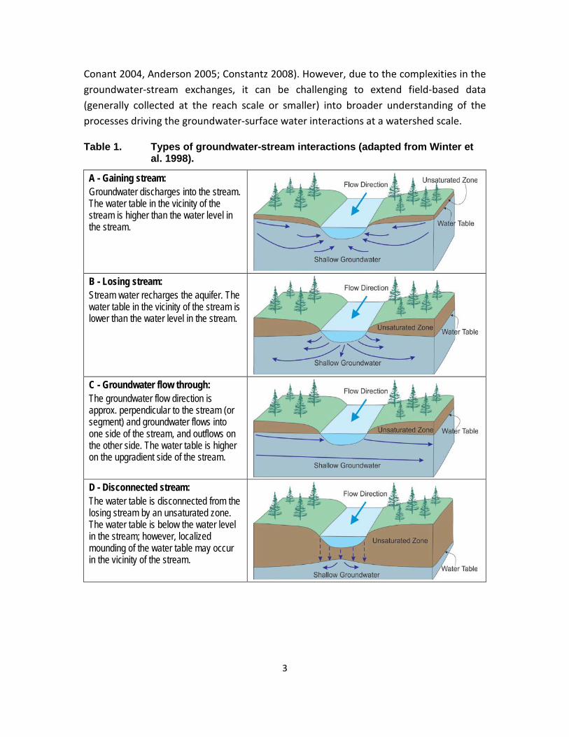
A useful approach for understanding the broader scale connectivity between an aquifer and a stream was proposed by Allen et al. (2010) who analyzed groundwater level responses in relation to streamflows in various temperate mountainous settings (British Columbia, Canada). They demonstrated that the coupled response of aquifers and streams can be reasonably predicted by considering the hydroclimatology and the “aquifer-stream system” type. The seasonal timing of the aquifer-stream system response depends on the hydroclimatology of the region; rainfall-dominated (pluvial) or snowmelt-dominated (nival) (Figure 1). A hybrid (mixture of rain and snow) hydroclimatology is also possible (not shown). These aquifer-stream system types were defined based on classifying different aquifer types (Wei et al. 2009). The magnitude and timing of the recharge and discharge response of the aquifer-stream system was shown to depend not only on the storage and permeability characteristics of the aquifer, as might be anticipated, but also on the aquifer-stream system type, which is broadly classified as diffuse recharge-driven or stream-driven (Allen et al. 2010).

1. Diffuse Recharge-Driven – the aquifer is recharged solely by precipitation and groundwater discharges to streams throughout the year as baseflow. These systems are commonly associated with first order streams.

2. Stream-Driven - groundwater flow to and from streams is bi-directional, and varies seasonally depending on stream stage. These aquifer-stream systems are found in association with major streams/rivers.

6

Figure 1. Framework for classifying the responses in aquifer-stream systems,

showing end members of the hydroclimatic regimes (from Allen et al. 2010 with permission).

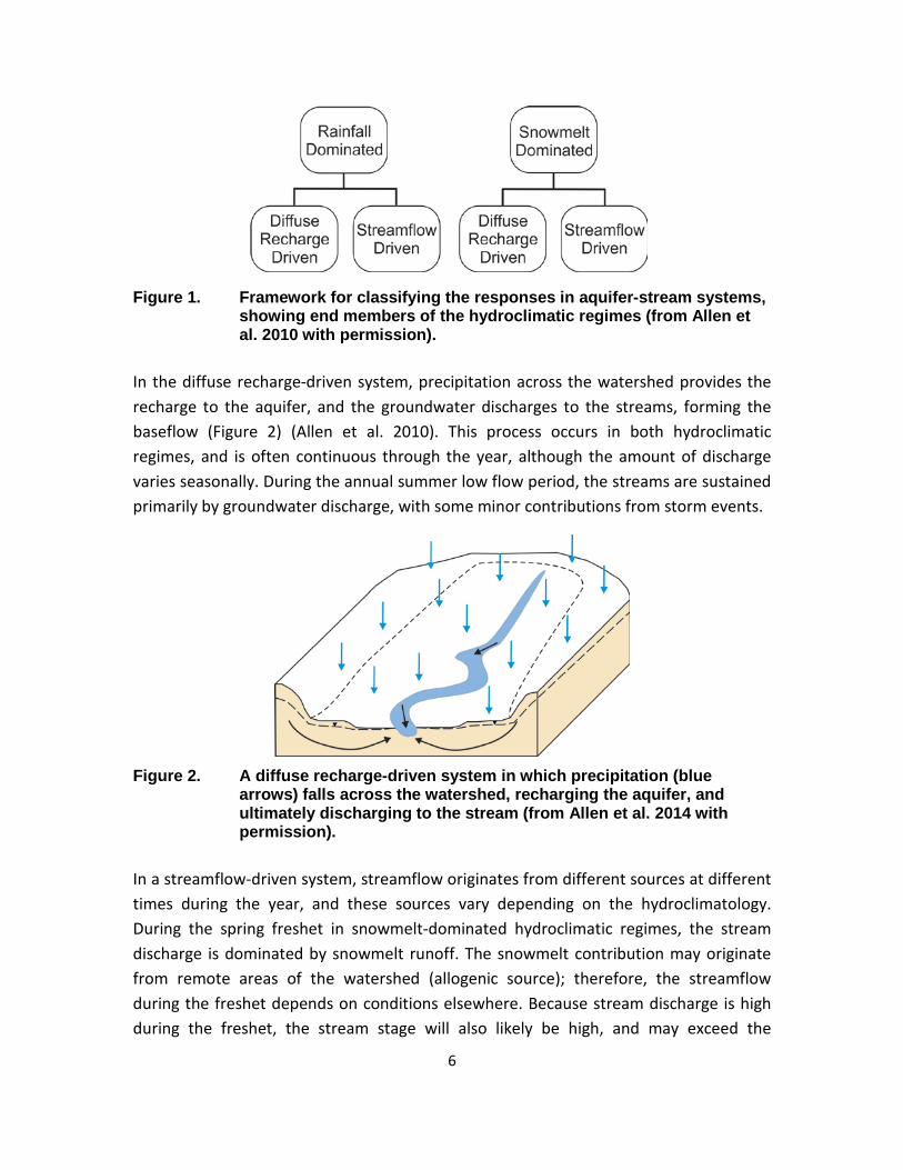
In the diffuse recharge-driven system, precipitation across the watershed provides the recharge to the aquifer, and the groundwater discharges to the streams, forming the baseflow (Figure 2) (Allen et al. 2010). This process occurs in both hydroclimatic regimes, and is often continuous through the year, although the amount of discharge varies seasonally. During the annual summer low flow period, the streams are sustained primarily by groundwater discharge, with some minor contributions from storm events.

Figure 2. A diffuse recharge-driven system in which precipitation (blue

arrows) falls across the watershed, recharging the aquifer, and ultimately discharging to the stream (from Allen et al. 2014 with permission).

In a streamflow-driven system, streamflow originates from different sources at different times during the year, and these sources vary depending on the hydroclimatology. During the spring freshet in snowmelt-dominated hydroclimatic regimes, the stream discharge is dominated by snowmelt runoff. The snowmelt contribution may originate from remote areas of the watershed (allogenic source); therefore, the streamflow during the freshet depends on conditions elsewhere. Because stream discharge is high during the freshet, the stream stage will also likely be high, and may exceed the

7

elevation of the water table in a valley aquifer. Therefore, during the freshet, the stream recharges the aquifer adjacent to the stream (Figure 3). This aquifer recharge mechanism is relatively short lived (less than a month in studied aquifers; Scibek et al., 2007). Following the freshet, when stream discharge reduces, the flow direction within the aquifer reverses and groundwater recharges the stream. Local precipitation (either rainfall or snowmelt) may also recharge the aquifer throughout the year, as shown by the blue arrows in Figure 3. During the summer low flow period, the main contribution to the stream is local groundwater discharge. The same processes occur in rainfall-dominated hydroclimatic regimes, with the exception that snowmelt is not a driver of streamflow.

Figure 3. A streamflow driven system, with the snowmelt-derived streamflow

recharging the aquifer adjacent to the stream (left). The blue arrows indicate precipitation across the aquifer contributing locally to the recharge. During the summer low flow period (right), groundwater discharge to the stream is driven by the local groundwater flow, which depends on diffuse recharge to the aquifer (modified from Allen et al. 2014 with permission).

In both aquifer-stream system types, streamflow is often sustained by the groundwater discharge during the summer low flow period. First order streams will be the most dependent on groundwater discharge from the local aquifers during the low flow season. Higher order streams, because they accumulate discharge from lower order streams up-gradient and thus are often larger, generally are less dependent on discharge from local aquifers. Therefore, the sensitivity of a stream to stressors in the aquifer (e.g. pumping) will depend on the stream discharge during the low flow season and the proportion of the discharge that derives from local groundwater discharge.

2.4 Stressors and Stream Vulnerability

Groundwater pumping in the vicinity of the stream is one of the most important stressors on an aquifer-stream system. Pumping can impact the various types of

8

groundwater-stream interactions shown in Table 1, with the exception of the disconnected stream, which is not directly impacted by pumping of groundwater3.

The potential effects of groundwater pumping on streamflow in an unconfined aquifer are presented in Table 2 (A through D). In a non-pumping situation (A), the shallow groundwater flows from recharge areas at higher elevation and discharges into the stream. The installation of a groundwater well, pumping at some rate (Q1) (B), draws groundwater from a capture zone around the well, and creates a cone of depression4. In this scenario, the pumping well intercepts a portion of the groundwater that would have otherwise discharged to the stream, leading to some lowering of the stream level. Under conditions of reduced recharge to the aquifer (C), perhaps due to climate change or land use change, the water table may be lower over a large area. Pumping under reduced recharge conditions would exacerbate the drawdown effect. At a higher pumping rate (Q2) (D), the water table is lowered further (compared to at Q1), and water may be drawn from the stream.

3 If the disconnection is temporary under natural conditions; prolonged pumping may lead to more permanent disconnection. 4 A cone of depression in an unconfined aquifer is a lowering of the water table in the vicinity of the well.

9

Table 2. Groundwater pumping effects on streamflow (adapted from Winter et al. 1998).

A - No pumping: Natural condition in a gaining stream with groundwater flowing from recharge areas at higher elevation and discharging to the gaining stream.

B - Pumping at a rate Q1 from a well near the steam: The pumping well draws water from a zone around the well (capture zone) and may intercept a portion of the groundwater that would have discharged to the stream.

C - Pumping at Q1 with lower recharge: The lower recharge leads to a lower water table, exacerbating the effects of drawdown.

D - Pumping at a higher rate Q2 from a well near the steam: The pumping well draws more water from a larger capture zone. Pumping can lower the water table in the vicinity of the stream, and water may be drawn from the stream to meet the higher pumping demand.

The size of the cone of depression in an unconfined aquifer depends on the aquifer transmissivity (T) and specific yield (Sy). When T and Sy are low, the water table may lower substantially in a localized area around the well during pumping. In contrast, when T and Sy are high, for the same pumping rate, there is less drawdown near the well, and drawdown is distributed over a larger area. An aquifer with high T and Sy values is productive and also generally well connected to the stream; therefore, if a well is pumped at a high rate near the stream, there is a strong potential for the capture

10

zone to intersect the stream in a relatively short period of time; although the high aquifer productivity may limit the amount of water sourced from the stream (Winter et al. 1998; Alley et al. 1999; Barlow and Leake 2012). An aquifer with lower T and S values is not as productive, and a well placed near the stream may only derive some of its water from the stream over the same period of time due to the lower T. But in this case, a deeper cone of depression will form, and over time, this scenario would result in more water being sourced from the stream to meet the pumping demand.

Pumping from a confined aquifer in the vicinity of a stream may or may not have an impact on stream levels. Pumping causes a zone of depressurization (a lowering of the hydraulic head) in the vicinity of the well, which causes groundwater to move towards the well in much the same way as in an unconfined aquifer (Alley et al. 1999; Barlow and Leake 2012). The size of the zone of depressurization depends on the T and the storativity (S) 5 of the confined aquifer. While confined aquifers are oftentimes disconnected from surface water bodies, lowering of the hydraulic head in a confined aquifer can induce leakage from overlying unconfined aquifers, resulting in a lowering of the water table, and therefore, an indirect impact on stream level as discussed above for unconfined aquifers. Connection between a stream and a confined aquifer may occur if the stream is incised into the confining layer, or if the aquifer outcrops along the stream channel.

Other stressors include potential changes in the timing and amount of precipitation as a result of climate change. Such changes have the potential to lead to more extreme summer low flow events, and to extend the length of the summer low flow period in many streams (Déry et al. 2009). Climate variability and climate change also have the potential to impact aquifer recharge (e.g. Allen et al. 2004) as well as lead to increased water resource demands (e.g. Cohen et al. 2004), which in turn will lead to changes in groundwater conditions. Changes in land use/land cover (urbanization, timber harvesting, etc.) also impact recharge (Arnell 2002).

Understanding the likely response of streams to changes in the groundwater conditions is important for management of water resources, and for evaluating the potential impacts from the various stressors described above, particularly pumping. However, generalized frameworks for evaluating the vulnerability of streams to changes in the aquifer are currently lacking. For jurisdictions like British Columbia, which for the first time will be licensing groundwater under the new Water Sustainability Act (Bill 18: WSA, 2014) consideration of the impacts to streams due to groundwater pumping is of critical 5 S is much smaller than Sy; therefore, the same amount of pumping will result in a much larger cone of depression in a confined aquifers compared to an unconfined aquifer.

11

importance. To develop such a framework, however, would require information on groundwater – stream interactions for different geographical regions. In most regions, data are often available for other applications, such as aquifer characteristics compiled for aquifer inventory, surface water data, and fish habitat metrics. These data available may not be ideal for the representation of groundwater – stream interactions; however; they represent a valuable resource that can be repurposed for evaluation of stream vulnerability.

3 Vulnerability Assessment for Groundwater Dependent Streams: Overview

The Vulnerability Assessment involves a three level assessment procedure shown schematically in Figure 4:

Figure 4. Overview of the levels of assessment for Stream Vulnerability.

12

3.1 Level I Assessment

A Level I Assessment evaluates the potential vulnerability of a stream based on the hydrologic setting and the level of development of the aquifer. The assessment is qualitative and relies on existing publicly available information for classified aquifers in BC. A Level I Assessment is intentioned for screening or prioritizing purposes or for provincial level classification of stream-aquifer connectivity in diverse settings. If a Level I Assessment determines the stream is potentially vulnerable, then a Level II Assessment would be undertaken.

3.2 Level II Assessment

A Level II Assessment rates the vulnerability of the stream relative to other streams, specifically the degree of connectivity between the stream and the aquifer, and the stressor(s) that act on the system. This Level II Assessment is semi-quantitative and is intended for establishing water management guidelines or policies in aquifers where the stream is connected to the aquifer system. If a Level II Assessment determines the stream is vulnerable, a Level III assessment would be undertaken to quantify the potential impact to the stream from the stressor(s).

3.3 Level III Assessment

A Level III Assessment considers the impacts to the stream from groundwater-related stressors. Level III Assessments are quantitative in that they incorporate data analysis requiring more specific information about how the stream-aquifer system functions as well as the magnitude of the stressors acting on the system. Level III Assessments are site specific and intended for such activities as drought preparedness, groundwater licensing, planning of subdivisions, etc. The assessment aims to demonstrate the likely impact on a stream due to stressors acting on the aquifer system. The assessment could include, for example, the impact of groundwater pumping or impacts due to changes in recharge rates caused by land use/land cover changes or climate change/climate variability.

4 Level I Assessment: Potential Stream Vulnerability

A Level I Assessment evaluates the potential vulnerability of a stream based on the hydrologic setting and the level of development of the aquifer in the area of interest. The main objective of a Level I Assessment is to assess whether the stream is potentially connected to the aquifer, and whether the aquifer can produce adequate quantities of

13

water to meet the current demand. A Level I Assessment is intended for screening or prioritizing purposes, or for provincial level classification of stream-aquifer connectivity in diverse settings.

A Level I Assessment uses publicly available information, where possible, on aquifers and streams. Spatial data can be accessed from iMapBC (http://maps.gov.bc.ca/ess/sv/imapbc/ ).

4.1 Step 1: The Hydrologic Setting

Step 1 of the Level I Assessment establishes whether the stream intersects the aquifer. The BC Ministry of Environment maintains an inventory of aquifers in the province. Aquifer polygons have been mapped, and their attributes (outline, vulnerability, among other para meters available for specific aquifers) characterized. All aquatic-related features (streams, rivers, lakes, wetlands, etc.) are also mapped at a 1:50,000 scale for the province (BC Watershed Atlas -http://www.env.gov.bc.ca/fish/watershed_atlas_maps/). If the stream intersects an aquifer, then there is a potential for that stream to interact with the aquifer. Some examples are provided below.

Figure 5 shows the aquifer polygons in the Fraser Valley with a stream map layer based on the BC Watershed Atlas (Stream Routes 50k). Figure 6 shows an enlarged portion of Figure 5. In both figures, most of the streams intersect an aquifer polygon. Not all aquifers are at the surface, so these figures identify only potential interactions.

http://maps.gov.bc.ca/ess/sv/imapbc/

http://www.env.gov.bc.ca/fish/watershed_atlas_maps/

14

Figure 5. Aquifer polygons (black outline) shown with streams (blue) in the

Fraser Valley.

Figure 6. Zoomed view of aquifer polygons (black outline) with streams (blue)

in the Fraser Valley.

15

Figure 7 shows the aquifer polygons in the Fraser Valley with the map layer of streams designated as Sensitive Streams in the Fish Protection Act. In catchments with sensitive streams, a Level II Assessment is recommended.

Figure 7. Zoomed view of aquifer polygons (black outline) with streams (blue)

and designated sensitive streams (Fish Protection Act) in the Fraser Valley.

4.1.1 Other Considerations

In some cases, there may be insufficient information available on iMapBC to undertake step 1 of the Level I Assessment and it is recommended a hydrogeologist be consulted in those situations.

Not all streams intersect aquifers. For example, confined aquifers typically lie at depth below the surface, and while they are mapped and appear to be at surface based on the aquifer polygons, further investigation would be needed to determine if an aquifer is unconfined or confined. Also, a number of aquifers mapped as confined aquifers are semi-confined by semi-permeable and/or discontinuous confining units. Those aquifers mapped as confined, therefore, should be investigated to determine potential for connectivity with streams.

16

Not all aquifers are mapped. While some 1,000 aquifers have been mapped to date in the province, not all aquifers have been mapped. If aquifer polygons are not shown for the area of interest, then further investigation is needed to obtain the data necessary to complete a Level I Assessment.

Aquifer polygons in bedrock regions typically do not extend beyond areas with water wells. In bedrock regions (areas with no substantial accumulation of surficial materials), aquifer polygons typically extend no further than the area with existing water wells. This is because the aquifer inventory focuses on developed areas. However, even a single well placed outside an aquifer boundary in bedrock has the potential to be connected to a stream. If aquifer polygons in bedrock do not extend to the area of interest, then further investigation is needed.

4.2 Step 2: Potential Stream Vulnerability

Step 2 of the Level I Assessment is based on the BC Aquifer Classification System (ACS) (Kreye and Wei 1994). The system 1) classifies aquifers on the basis of their Level of Development and vulnerability to contamination, and 2) provides ranking values for aquifers using hydrogeologic and water use criteria. While designed primarily for assessing the vulnerability of the aquifer to contamination from surface activities, the Level of Development component is readily adapted to assess stream vulnerability as it relies on information on the aquifer properties. Thus, for a Level I Assessment, the Level of Development directly represents the Potential Stream Vulnerability.

The Level of Development is a relative and subjective term. However, it enables comparison of the amount of groundwater withdrawn from an aquifer (demand) to the aquifer’s inferred ability to supply groundwater for use (productivity) (Berandinucci and Ronneseth 2002). In the context of stream interaction, aquifers with a higher Level of Development are more likely to impact streamflow than those with a low Level of Development, other factors being equal. The Level of Development is assessed based on 1) aquifer productivity and 2) groundwater demand. Aquifer Productivity and Groundwater Demand have been assessed for over 1,000 aquifers in BC as part of the aquifer inventory process (BC Ministry of Environment, 2014).

4.2.1 Aquifer Productivity

Aquifer Productivity describes the rate of groundwater flow from wells and springs and the abundance of groundwater in an aquifer. Indicators of productivity (e.g., aquifer material, reported well yields, specific capacity of wells, and transmissivity of the aquifer) are used to infer potential water availability of the aquifer (Table 3). For

17

example, Kreye and Wei (1994) assign an indicator of 1 to a low productivity aquifer, 2 for moderate, and 3 for high (Table 3). Figure 8 shows an example of aquifers in the Fraser Valley for which productivity has been estimated.

Table 3. Productivity classes (from Kreye and Wei, 1994).

Indicators of Productivity

Class Low (1) Moderate (2) High (3)

Aquifer Material -Silt and sand -Fractured bedrock

Sand Sand and gravel

Well Yield (L/s) < 0.3 0.3 – 3.0 > 3.0 Specific Capacity (L/s/m)

< 0.4 0.4 – 4 > 4

Transmissivity (m2/s) < 5.0E-4 5.0E-4 - 5.0E-3 > 5.0E-3

Figure 8. Productivity (Low (1), Moderate (2), High (3)), of aquifers in the

Fraser Valley with an overlay of sensitive streams (pink).

4.2.2 Groundwater Demand

The Groundwater Demand provides information on the groundwater use. Well use and actual withdrawal rates are usually not available. Therefore, groundwater demand is generally assessed subjectively based on domestic well density per map quadrant, the

18

number and type of production wells, and general knowledge of well use and land use in the area (Table 4). Figure 9 shows an example of aquifers in the Fraser Valley for which demand has been estimated.

Table 4. Demand classes (modified from Kreye and Wei, 1994).

Demand Classes Class Low (1) Moderate (2) High (3)1

Well Density Descriptor

Low Moderate High

Number of Wells < 10 10-50 >50 Well Density (wells/km2)

< 4 4-20 >20

1The high and very high categories from Kreye and Wei (1994) have been combined in this table. Aquifers categorized as very high well density in the aquifer database are simply classified high in this table.

Figure 9. Groundwater Demand (Low (1), Moderate (2), High (3)) in the Fraser

Valley with an overlay of sensitive streams (pink).

4.2.3 Potential Stream Vulnerability

The Potential Stream Vulnerability (Table 5) is derived from the Level of Development defined by Berardinucci and Ronneseth (2002). Three ranks of Potential Stream

19

Vulnerability are designated: Low (1); Moderate (2); or High (3), and based on the categories defined in Berardinucci and Ronneseth (2002) the rank may range for different combinations of Demand and Productivity. The range is represented by the color scale in Table 5.

Table 5. Potential Stream Vulnerability risk matrix.


Where an aquifer has not yet been classified, the Aquifer Productivity and Level of Demand can be assessed using the tables above following the methodology by Berardinucci and Ronneseth (2002). Indicators of Aquifer Productivity and Level of Demand can be estimated using information on wells in the BC WELLS database, which is also linked to iMapBC.

Where the Potential Stream Vulnerability risk matrix results in two possible ranking outcomes (e.g. II-III in Table 5), additional information may be required for assigning a final ranking and action required (Table 6). The following list provides various options; the list is not exhaustive, but rather acknowledges some of the challenges.

• A conservative approach would be to apply the higher ranking by default. • Consider additional aquifer properties for each aquifer – stream system, such as:

o Aquifer type (listed in Table 7), with Type 1a resulting in a lower ranking due to its proximity to a higher order stream or river and so development may have less impact on streamflow. Other aquifer types listed as commonly connected to streams would be ranked higher;

o Relative area of stream segments per area of aquifer; o Relative position of the aquifer, with confined aquifers having a lower

rank and unconfined aquifers having a higher rank;

Low (1) Moderate (2) High (3)Low (1)

ModerateLow - Moderate

Low

Moderate (2) Moderate - High

ModerateLow - Moderate

High (3)High

Moderate - High

Low to High

ProductivityDe

man

d

20

o If the depth to water in the confined aquifer (based on available well records) indicates upward flow (higher head at depth), a lower ranking for that aquifer would be assigned;

o A higher ranking would be assigned to aquifers that have a quantity concern identified in the aquifer inventory, and;

o Higher weighting could be assigned to groundwater demand, with low demand aquifers ranked lower.

4.2.5 Final Level I Assessment Criteria

Table 6 lists the criteria that are used to determine the action required depending on whether the stream intersects the aquifer in the area of interest and Level of Development within the aquifer in the area of interest.

Table 6. Potential Stream Vulnerability within an aquifer and action required.

Potential Stream

Vulnerability

Description Action Required

Low (1) No stream intersects the aquifer in the area of interest. Thus, there is a low potential for connection between the stream and the aquifer. Demand for water is light relative to water availability.

No further action required

Moderate (2) A stream either passes through the aquifer or borders the aquifer. Thus, there is a moderate potential for connection between the stream and the aquifer, particularly in areas very close to the stream. Demand for water is moderate relative to water availability.

Proceed to Level II Assessment

High (3) A sensitive stream either passes through the aquifer or borders the aquifer and/or there is a high potential for connection between the stream and the aquifer. Demand for water is high relative to water availability.

Proceed to Level II Assessment

21

5 Level II Assessment: Rating Stream Vulnerability

5.1 Overview

A Level II Assessment results in a rating of stream vulnerability. It is a semi-quantitative assessment process that relies on understanding of the physical system (the aquifer - stream system), and what current stressors act on the system. A Level II Assessment rates the stream vulnerability relative to other streams, specifically the degree of connectivity between the stream and aquifer, and is intended for establishing water management guidelines or policies in aquifers where the stream is connected to the aquifer system.

The Stream Vulnerability (SV) is the combination of the Stream Susceptibility (SS) and the Hazard (H) (Figure 10) and is rated in a matrix. The stream susceptibility evaluates the potential for the stream to be influenced by stressors acting on the aquifer system. It is based on the aquifer characteristics and the recharge to the aquifer system. The hazards represent the current stressors to the aquifer, specifically pumping, which may translate into potential changes to the stream.

Figure 10. Flow chart outlining the components of stream vulnerability.

5.2 Stream Susceptibility (SS)

The stream susceptibility (Equation 1) represents the natural hydrogeological system, characterized by the aquifer setting, the aquifer properties, the nature of the interconnection between the aquifer system and the stream, and the recharge characteristics:

Stream Susceptibility (SS) = Aquifer Characteristics (A) * Recharge Ratio (QS/QR) (1)

22

5.2.1 Aquifer Characteristics (A)

Wei et al. (2009) summarize the characteristics of the major aquifer types in the province. The aquifer characteristics reflect the aquifer setting, the origin and type of geologic deposit, the degree of confinement, and the potential hydraulic connection with surface water. There are twelve aquifer types, eight in unconsolidated sand and gravel settings, and four in bedrock (Table 7).

Each aquifer type is defined primarily on geological and hydrological properties, as well as on practical considerations, such as data availability (Wei et al. 2009). The main geologic factors are the origin and type of the geologic deposit that comprise an aquifer (e.g., sand and gravel aquifer forming a delta at the mouth of a river, or a plutonic granitic fractured bedrock aquifer). The origin and type of geologic deposit often governs an aquifer’s hydraulic properties, such as the nature of the porous medium (porous sand and gravel, or fractured bedrock) and its ability to transmit and store water. The degree of aquifer confinement represents the hydraulic separation of aquifers from each other and from surface waters. Aquifers can be unconfined, discontinuously confined, partially confined, or confined. Unconfined aquifers have the highest likelihood of being connected to the stream because there is no low permeability layer separating the aquifer from the stream. Deep confined aquifers are the least likely to be connected to streams.

Table 7 rates each aquifer type according its likely connection with a stream. The rating scheme is also shown in Figure 11. A direct hydraulic connection can be disadvantageous to streamflow because pumping could induce infiltration of surface water into the aquifers, and thereby remove water from the stream.

Table 7. Aquifer types and key hydrogeological characteristics (from Wei et al. 2009) with the assigned Aquifer Characteristics (A) ratings assigned through consultation with BC Ministry of Environment.

Aquifer type Confined - unconfined

Connection with streams

Rating1

1. Aquifers of fluvial or glaciofluvial origin along river valley bottoms

Unconfined

a. aquifers along low gradient, higher order rivers

Unconfined Commonly connected but stream size buffers impact

4

b. aquifers along generally higher gradient, moderate order rivers

Unconfined Commonly connected

10

c. aquifers along lower order streams; Unconfined Commonly 10

23

Aquifer type Confined - unconfined

Connection with streams

Rating1

limited aquifer thickness and lateral extent

connected

2. Deltaic (sand and gravel) aquifers Unconfined Commonly connected

10

3. Alluvial, colluvial (sand and gravel) fan aquifers

Unconfined Commonly connected near the stream

8

4. Aquifers of glacial or pre-glacial origin

Variable

a. Outwash and ice-contact sand and gravel aquifers (glacio-fluvial)

Unconfined Commonly connected near the stream

8

b. Aquifers of glacial or pre-glacial origin

Mostly confined

Possibly connected if unconfined

4

c. Confined aquifers of glacio-marine origin

Confined Unlikely to be connected

4

5. Sedimentary rock aquifers Variable a. fractured sedimentary rock aquifers Unconfined

near surface Possibly connected near the stream

3

b. karstic limestone aquifers Unconfined near surface

Likely connected 5

6. Crystalline rock aquifers Variable a. flat-lying or gently-dipping volcanic flow aquifers

Unconfined near surface

Likely connected 5

b. fractured igneous intrusive, metamorphic, fractured volcanic or metavolcanic aquifers

Unconfined near surface

Possibly connected near the stream

3

1The ratings were determined based on expert knowledge of aquifer types in British Columbia. Intermediate rating values could be assigned based on local hydrogeological conditions.

24

Figure 11. Overview of Aquifer Characteristics rating.

25

5.2.2 Recharge to Stream (QR)

The recharge component applied to assess the reliance of the stream during the summer low flow period on locally-derived aquifer recharge. Annual recharge is assessed based on the area contributing groundwater discharge to the stream, and is compared to baseflow to estimate the ability of the discharge amount to sustain the streamflow.

When considering the annual summer low flow period, the annual recharge to the aquifer is a critical factor. Aquifer recharge, however, is difficult to quantify due to large uncertainties in the various water balance components. Equation2 shows a typical annual water balance equation for an aquifer system.

R = (P + Qin + GWin) – (AET + Qout + GWout) ± ΔSG ± ΔSS (2)

where R is the recharge, P is precipitation, Qin is the surface water inflow (influent water bodies), GWin is the groundwater inflow to the area (from adjacent areas and return flows from irrigation), AET is actual evapotranspiration, Qout is the surface water outflow (effluent water bodies), GWout is the groundwater outflow from the area (to adjacent areas and pumping), and ΔSG ± ΔSS are the changes in storage for each of groundwater and surface water (typically assumed to be zero on an annual basis). Quantification of each component of the water balance equation for the aquifer system requires data and a sound understanding of the system. For this reason, a full water balance assessment would require a Level III Assessment.

For a Level II Assessment, the water balance of the aquifer is approximated as follows:

R = P – PET = QR (3)

This water balance equation is a gross simplification of the aquifer system, but it provides a first order approximation of the potential recharge (R) and hence the discharge to the stream from the aquifer system (QR). Equation 3 assumes the aquifer drains to a stream and that all the recharge to the aquifer discharges to the stream (R = QR). It assumes no pumping. It assumes that if there is any groundwater inflow from adjacent areas, that this groundwater leaves the aquifer through adjacent areas. It also assumes that there are no gains to the aquifer from the stream.

Precipitation is measured at many locations in Canada, and annual estimates are available as precipitation normals over a recent 30 year period (Environment Canada 2007). BC station data are also available from the Data Portal maintained by the Pacific

26

Climate Impacts Consortium (http://www.pacificclimate.org/data/bc-station-data). In addition to the Environment Canada stations, data for many non-federal climate stations are available. Near real-time climate data are available. The quality of the data used for a Level II Assessment must be balanced with the availability of data (e.g. period of record, seasonal availability) and proximity to the area of interest. For example a close proximity climate station with high quality data, but at high elevation may not be appropriate for evaluating a valley bottom aquifer due to orographic effects and greater snowfall, such that a climate station with poorer quality data but at a representative elevation might be more appropriate to use.

Estimates of actual evapotranspiration (AET) are often not available due to limited measurements. For this reason, the potential evapotranspiration (PET) is used in this assessment. PET, however, generally overestimates AET because it does not consider the available water. The PET values can be derived using the FAO Penman-Monteith method, which is considered one of the more comprehensive PET estimation methods (Hess 1996, Herrera-Pantoja and Hiscock 2008). The FAO Penman-Monteith method for reference crop evapotranspiration requires air temperature, wind speed, radiation, and humidity (Allen et al. 1998). The full suite of these parameters may not be readily available at some climate stations; therefore, it is possible to estimate PET from using a simplified approach that requires the daily solar radiation (SR) and maximum air temperature (Tmax) (Equation 4) (Cohen et al. 2004).

-3.26 + 0.201Tmax + 0.058 SR = PET (4)

Solar radiation can be calculated for the days of the year using the solar position and radiation calculator (Washington State Department of Ecology, 2014), using longitude/latitude and elevation.

When summed over the year, PET can exceed precipitation, specifically in arid or semi-arid areas. For this reason, R was calculated daily. If precipitation occurred on a particular day, a recharge amount was computed according to Equation 3. If there was no precipitation, then R was assumed to be zero. This approach likely overestimates R, because soil moisture is able to evaporate and plants are able to transpire even on days it does not rain; however, for a Level II Assessment, recharge calculated in this way is a first approximation.

Using values for P (mm/yr) and the calculated values of PET (mm/year) for the aquifer area (m2), R or QR (m3/year) is estimated. The aquifer area corresponds to the area contributing to streamflow measured at a gauging station (see below). For simplicity,

http://www.pacificclimate.org/data/bc-station-data

27

the aquifer area can be considered the same as the watershed or catchment area. This definition assumes that all the recharge within the watershed exits the watershed via the stream. Any deep groundwater flow is neglected.

5.2.3 Summer Streamflow (QS)

QR represents the volume of groundwater that discharges to the stream on an annual basis as baseflow. Ideally, the baseflow would be calculated from the same period of record as the climate normals. While there are hydrograph separation techniques that can be used to estimate the baseflow, which varies seasonally, the approach used here is to calculate the average summer streamflow, QS, (from July to September) over the period of record. In actuality, the summer streamflow will include the baseflow as well as storm runoff from rain events, and so may overestimate summer baseflow. But, countering this is the fact that summer baseflow is less than the average annual baseflow. Therefore, summer streamflow (QS) is considered a reasonable approximation to baseflow.

5.2.4 Recharge Ratio (QS/QR)

The Recharge ratio QS / QR represents the proportion of the summer streamflow that derives from groundwater recharge. There are three main outcomes for this ratio: 1) If the summer streamflow is fully dependent on groundwater recharge, the ratio will be one, and the stream would be considered sensitive to the amount of recharge in the aquifer. 2) If QS is larger than QR, then streamflow likely derives from an area remote to the aquifer, such that the streamflow is augmented by upstream contributions. 3) if QS is smaller than QR, then what small contributions of recharge to the streamflow there are must be significant, and the stream is considered sensitive. The rating scheme for Recharge Ratio is shown in Table 8. The maximum and minimum ratings were determined from the highest and lowest likely recharge ratios expected in British Columbia. The intermediate values were assigned according to order of magnitude changes in the recharge ratio to best capture the observed ranges during testing of the method.

28

Table 8. Recharge Ratio (QS/QR), and the assigned ratings.

Ratio (QS/QR) Rating > 1000 1 > 100 2 > 10 3 1.0 - 9.9 4 0.1 – 0.9 5 0.01 – 0.09 6 0.001 – 0.009 7 0.0001 – 0.0009 8 0.00001 – 0.00009 9 < 0.00001 10


Climate varies spatially. In large watersheds or in watersheds with elevation changes, the precipitation (P) and temperature can be quite different from one area to another. For example, measurements of P at valley bottom climate stations generally underestimate P at higher elevation due to orographic effects. If climate is known to vary spatially, the climate data should be interpolated or zoned appropriately to estimate recharge (R).

Climate varies interannually. Precipitation and temperature vary from year to year, and at longer time scales due to climate oscillations such as the El Nino Southern Oscillation (ENSO), the Pacific Decadal Oscillation (PDO), among others, and is expected to have effects on groundwater and watershed hydrology in BC (Fleming and Quilty 2006; Merritt et al. 2006; Scibek and Allen 2006a; Pike et al. 2010). Recharge calculations could incorporate potential climate variability by using historic records where available. Recharge calculated using historic high and low values rather than annual averages would provide a means to assess the sensitivity of recharge to climate variability in the assessment. Many methods are discussed in the literature for estimating climate change impacts on groundwater recharge; however, adopting these approaches is non-trivial and would best be carried out under a Level III Assessment. Some areas of BC have climate change impacts on recharge assessed and these estimates of future recharge could be used in a Level III Assessment. (e.g. Scibek and Allen 2006 (Grand Forks); Toews et al. 2009 (Oliver); Foster and Allen 2015 (Cowichan Watershed). In areas where climate change impacts are identified as a factor contributing to high stream susceptibility, a Level III Assessment is recommended to address site specific outcomes.

29

Summer streamflow (QS) varies interannually. For similar reasons as above for recharge, a range of QS values corresponding to the same years used to estimate the range of QR values (as above) could be used.

The rating for the recharge component of stream sensitivity could be based on other criteria. For example, if the instream flow needs (QINF)for a particular stream are known, QR could be compared to QIFN.

Other measures of the relative importance of groundwater recharge to streamflow include the baseflow index (BFI), which is defined as the ratio of annual baseflow in a river to the total annual runoff. BFI values for different streams could be compared in different areas of the province and these values used to rate different streams. The baseflow of the stream can also be estimated using simple hydrograph separation techniques rather than QS, and use of an alternate method is required if the low flow period being evaluated is not the summer period.

5.2.6 Stream Susceptibility (SS) Rating

The Stream Susceptibility (SS) rating is calculated as the product of the Aquifer Characteristics (A) rating and the Recharge Ratio (QS/QR) rating. The overall SS rating will range from 3 – 100. The rating scheme for Stream Susceptibility is shown in Table 9.

Table 9. Stream Susceptibility (SS), and the assigned ratings.

Recharge Ratio (QS/QR) Low (1-3) Moderate (4-7) High (8-10)

Aqui

fer C

hara

cter

istics

(A)1

Low (1-3)

Low Low Low Low Low Low Low Mod Mod Mod

Low Low Low Low Low Mod Mod Mod Mod Mod

Moderate (4-7)

Low Low Low Mod Mod Mod Mod Mod Mod Mod

Low Low Mod Mod Mod Mod Mod High High High

High (8-10)

Mod Mod Mod Mod Mod Mod High High High High

Mod Mod Mod Mod High High High High High High

1Ranges for Aquifer Characteristics (A) are continuous in this table, but in Table 7 they are not continuous.

30

5.3 Hazard (H)

The Hazard (H) component of stream vulnerability represents the primary stressor to the aquifer system, i.e., pumping (Equation. 5). For the purpose of a Level II Assessment, the H component is considered representative of current conditions. Future stressors are evaluated in a Level III Assessment, and could include land use/land cover changes, climate variability and climate change, which can lower the net recharge, and increased groundwater extraction.

H represents the magnitude and likelihood that the hazards that may change the water quantity in the stream:

Hazard (H) = Groundwater Pumping Magnitude * Likelihood of Impact (5)

The Groundwater Pumping Magnitude is assessed based on the volumetric pumping rate. The Likelihood of Impact is based on the ratio of the pumping volume to the recharge to the stream. The volumetric pumping rate is assessed for either the area of aquifer polygon, or the area of the stream watershed.

The annual volume of groundwater pumped is then compared to the Recharge to stream (QR), as calculated in Equation 3. If QP is equal to, or greater than, QR, the pumping is very likely impacting the streamflow quantity and represents a hazard. If QP is less than the QR, pumping may not be impacting the stream; however, the magnitude of the ratio between the two components provides an indication of the condition of the system.


For establishing water management guidelines or policies, a sensitivity analysis should be conducted whereby the effect on the assessment results are compared for different Hazard magnitudes (increasing the number of wells in the zone). This is necessary for two reasons: 1) The Province estimates that perhaps only 50% of wells are recorded in the WELLS database; therefore, the number of active wells may be significantly underestimated; and 2) The assessment would better reflect how sensitive the results are for current conditions. If there is a noticeable change in H rating, then the system is particularly sensitive to the number of wells.

The Level II Assessment utilizes the actual pumping rate (if known) or the estimated yield of the well, when reported in the WELLS database. If no information is available from the WELLS database on estimated well yield, then the well can be assumed to be

31

pumped at the domestic rate of 2,270 L/day, which is defined within the BC Well Protection Toolkit as the estimated water use per household (BC Ministry of Environment 2004). If possible, all wells in the area of interest should be included. A door-to-door survey may be required to identify the well location and the pumping rate.

The Level II Assessment assumes that the pumping rate is constant. Seasonal changes in water use are not accounted for. The Level II Assessment also assumes all the groundwater pumped is removed from the aquifer. Return flows (e.g. irrigation and septic fields) are not accounted for.

5.3.2 Hazard (H) Rating

The Hazard (H) rating is derived directly from the QP/QR ratios. Table 10 shows the Hazard (H) rating for a range of QP/QR ratios. Intermediate ratings are scaled accordingly.

Table 10. Ratio of volume pumped (QP) to the recharge to stream (QR) and the assigned ratings.

Ratio (QP/QR) H Rating < 0.19 Low (1) 0.2 – 0.39 Low (2) 0.4 – 0.59 Moderate (4) 0.6 – 0.79 Moderate (6) 0.8 – 0.99 High (8) > 1 High (10)

5.4 Final Level II Assessment for Stream Vulnerability (SV)

The Stream Vulnerability (SV) ratings can range from low to high, based on the Stream Susceptibility rating and the Hazard rating in Tables 9 and 10, respectively. Table 11 shows the Stream Vulnerability ratings as a matrix, which captures both components of the assessment.

Table 11. Stream Vulnerability (SV) matrix.

Stream Susceptibility

Low Moderate High

Haza

rd

Low Low Low Moderate Moderate Low Moderate High

High Moderate High High

32

Table 12 describes the whether or not further assessment is required based on the stream vulnerability rating.

Table 12. Stream Vulnerability (SV) rating and assessment required.

Stream Vulnerability

Rating

Description Action Required

Low The stream is currently of low vulnerability. No further action required unless there is a significant change to the water demand. A Level II Re-Assessment would then be required.

Moderate The stream is currently of moderate vulnerability.

No further action required unless there are changes to the water demand or the recharge conditions. A Level II Re-Assessment would then be required.

High The stream is currently of high vulnerability. Proceed to Level III Assessment

5.4.1 Example Level II Assessment

Level II Assessments were completed for nine streams in BC to represent different aquifer-stream settings in the province (Figure 12).

• Fishtrap and Bertrand Creeks - These creeks drain the Abbotsford aquifer in the Lower Fraser Valley in the Abbotsford aquifer. The aquifer-stream system is diffuse recharge-driven in a rainfall dominated hydroclimatic regime. Topographic relief is low. The aquifer is comprised of sands and gravels.

• The Kettle River Section at Grand Forks – The Kettle River meanders through the Grand Forks valley in south-central BC. The river originates at high elevation remotely to the valley. The aquifer-stream system is stream-driven in a snowmelt-dominated hydroclimatic regime. Topographic relief in the valley is low. The aquifer is comprised of sands and gravels.

• Daves Creek – The creek is situated in Okanagan Basin. The aquifer-stream system is diffuse recharge-driven in a snowmelt-dominated hydroclimatic regime. Topography is steep. The aquifer is comprised of bedrock.

• Upper Mission Creek – The creek is situated in Okanagan Basin. The aquifer-stream system is stream-driven in a snowmelt-dominated hydroclimatic regime. In this section of Mission Creek, topography is moderately steep. The stream incises a mostly confined aquifer comprised of sands and gravels.

• Fulford Creek – The creek is situated on Salt Spring Island and has been designated as a Sensitive Stream. The aquifer is diffuse recharge-driven in a

33

rainfall-dominated hydroclimatic regime. Topography is moderately steep. The aquifer is comprised of bedrock.

• Cowichan River section in the lower Cowichan Valley – The river is situated in Cowichan Valley, Vancouver Island. The river originates at high elevation in the valley. The aquifer-stream system is stream-driven in a snowmelt-dominated hydroclimatic regime. Two aquifers were assessed for comparison:

o Aquifer 179 –Topography is moderately steep. Well records for the aquifer indicate 62 known wells. The aquifer is comprised of sands and gravels.

o Aquifer 186 – Topography is low. Well records for the aquifer indicate 222 known wells. The aquifer is comprised of sands and gravels.

• Kiskatinaw River section – The Kiskatinaw River bounds the west and northwest side of the aquifer. The aquifer-stream system is stream-driven in a snowmelt-dominated hydroclimatic regime. Topography is low. The aquifer is comprised of bedrock.

Figure 12. Location of the nine Level II case study aquifer – stream systems in

BC. The aquifers for each system are shown in pink.

34

For each example, climate data were obtained from the nearest Environment Canada climate station. Daily recharge was estimated from daily precipitation minus PET for days were precipitation occurred. With the exception of the Grand Forks River example, the watershed area upstream of the gauge was used for calculating QR. QS was calculated over the period of record for the nearest stream gauge downstream. The summary of the steps of the Level II Assessment are presented in Table 13.

Fishtrap and Bertrand Creeks are very similar in their physical settings, locations, and size (same Aquifer Characteristics rating); however, the lower discharge and higher pumping volume at Bertrand Creek leads to a higher overall Stream Vulnerability.

The Cowichan River aquifers are very similar in their physical settings and have the same Aquifer Characteristic ratings and Stream Susceptibility; however, the volume pumped from the aquifer is greater in Aquifer 186 and leads to a high Stream Vulnerability, compared with a low rating for Aquifer 179.

Fulford Creek is designated as a Sensitive Stream under the Fish Protection Act, but was rated as having a low Stream Vulnerability in this assessment. However, surface water extraction volumes, and fish population status and habitat conditions are other key components to the Sensitive Stream Designation and are not included in this assessment method, which is focuses on sensitivity to changes in groundwater.

A Level III Assessment would be recommended for Fishtrap Creek, Bertrand Creek, Kettle River at the Grand Forks aquifer, Daves Creek, Mission Creek, and Cowichan River Aquifer 186; all of which have high Stream Vulnerability ratings. The Stream Vulnerabilities are low for Fulford Creek, Cowichan River Aquifer 179 and the Kiskatinaw River, and no further action is required unless there is a change in the recharge or volume pumped, at which time a Level II Re-assessment would be required.

35

Table 13. Example of Level II Assessments for nine streams.

Fishtrap Creek

Bertrand Creek

Kettle River

Daves Creek

Mission Creek

Fulford Creek

Cowichan River

Kiskatinaw River

Aquifer 179 Aquifer 186 Aquifer # 015 015 158 473 461 722-723 179 186 593 Type 4A 4A 1B 6B 4B 6B 1B IA 5A Aquifer Characteristics Rating (A)

8 8 10 3 4 3 10 10 3

Precipitation (mm/yr)a 1619.5 1619.5 552.7 313 414.82 997.7 1379.1 1379.1 468.6 PET (mm/yr)b 479.5 478.5 579.3 313 538.3 424.1 499 499 355.1 Recharge (mm/yr)c 1563.3 1518.3 445.2 566.9 326.3 941.8 1305.2 1305.2 392.2 Area of watershed/aquifer (km2) 37.0 51.0 38.8 37.2 15.1 21.1 7.6 16.9 1150 QR (m3/yr) *106 57.8 77.4 17.3 21.1 4.93 19.9 9.9 22.1 45000 QS (m3/yr)d *106 1.80 0.29 401. .88 34.8 4.65 683. 683. 14700 Qs/QR 0.031 0.004 23.214 0.042 7.063 0.234 68.854 30.964 0.327 Recharge Ratio Rating (QS/QR) 6 7 3 6 4 5 3 3 5 Stream Susceptibility (SS) 48 56 30 18 16 15 30 30 15 Q P(m3/yr) *106 240. 122. 200 128 6.42 8.78 3.54 308 3.56 n (number of wells) 856 828 611 188 57 204 62 222 163 QP/QR 4.15 1.58 11.58 6.07 1.30 0.44 0.36 13.96 0.01 Hazard Rating (H) 8 8 10 8 8 4 2 10 1 Stream Vulnerability (SV) High High High High High Low Low High Low

a The climate data were for the period spanning 1990-2002 based on availability; b Estimated from Equation 5; c Recharge calculated only for days when precipitation occurred; d Stream discharge data were for the summer periods (July – Sept.) spanning 1980 to 2012 based on availability.

36


The Level II Assessment may require some assumptions or simplifications, based on the availability of data or the complexity of the aquifer-stream system. In completing the Level II Assessment for the nine example streams, some of complexities were encountered. These are described below. The list is not exhaustive, but rather acknowledges some of the challenges.

• Some streams intersect multiple aquifers.

o For Fulford Creek, both aquifers (Aquifers 722 & 723) are classified as bedrock. These aquifers were merged into a single shapefile in ArcGIS for this assessment.

o For Fishtrap and Bertrand Creeks, the dominant aquifer (Aquifer 015) was selected as the aquifer of interest.

o For the Kiskatinaw River, the aquifer with the greatest potential connectivity to the stream was selected (Aquifer 593). Here, some of the aquifer polygons were unconfined, while others were confined or located at depth.

• The recharge area for the aquifer-stream area can be defined by the watershed area or the aquifer area.

o The contributing area for a low order stream can be readily defined as the watershed area (e.g. Daves Creek).

o For higher order streams, and for systems where the flow originates remotely (such as the Kettle River), the aquifer area will be the more appropriate area to use.

o For bedrock aquifers, it is important to note that the mapped aquifer boundaries are defined according to whether wells are present or not. The bedrock extends beyond the mapped boundary. Therefore, the contributing recharge area must be carefully assessed based on available data (e.g. topography, geology).

• Some large aquifers may be bounded by multiple streams (e.g. Kiskatinaw River). In these situations, recharge to the aquifer does not discharge to a single stream. Therefore, the QS/QR ratio calculated in this assessment is likely underestimated and would require adjustment in the Stream Vulnerability calculation.

• Data periods for the climate and the stream flow should be selected for the same time span for comparison. For these example assessments, ten-year periods were used when available.

37

• To calculate the recharge, the latitude, longitude, and elevation are required as a single point. For the calculations, a middle point in the aquifer or watershed was selected.

6 Level III Assessment - Stream Impact

A Level III Assessment aims to quantify the impacts to the stream from groundwater-related stressors. The Level III Assessment evaluates streams that have been identified as having a potential connectivity with the surrounding aquifer and where the aquifer productivity may be insufficient to meet the current demand (Level I Assessment), and where the stream is determined to be highly vulnerable to stressors (Level II Assessment). Level III Assessments are quantitative in that they require more specific information about how the stream-aquifer system functions as well as the magnitude of the stressors acting on the system. The stressors can include, for example, groundwater pumping from wells in zones adjacent to a susceptible stream and/or changes in recharge due to land use/land cover change, climate variability or climate change. Level III Assessments are site specific and are intended for such activities as drought preparedness, groundwater licensing, planning of subdivisions, etc.

The main objective of a Level III Assessment is to demonstrate the likely impact on a stream due to stressors acting on the aquifer system. Therefore, quantitative assessment tools are needed. Such tools can range from simple analytical methods to sophisticated numerical hydrogeological models. The range of possible tools is quite large. Two examples are used to demonstrate how certain tools could be used for Summer Low Flow Impact Assessment: 1) a simple method based on the fixed radius capture zone of a single well, and 2) a numerical groundwater flow model of an aquifer.

6.1 Well Scale: Well Capture Zone Analysis

Delineation of well capture zones is a critical component of any well vulnerability study. In the simplest of terms, a well capture zone visually represents the area (or volume) of aquifer that the well receives its water from (Hemmer and Beach 1997; BC Ministry of Environment 2004). By defining a well capture zone, decisions can be made to mitigate risk to the well, for example, eliminating hazardous land use activities within the capture zone area that may result in the well becoming contaminated. In the context of interactions with streams, well capture zones identify if the well likely receives water from the stream as it pumps. Capture zones normally are constructed for different periods (e.g. 60 day capture zone, 5 year capture zone, etc.) to reflect the time of travel

38

time of the water (or contaminant). For the purpose of a Level III Assessment, the time of travel is equivalent to the summer low flow period (in days).

Three methods of increasing complexity can be used to estimate well capture zones: 1) calculated fixed radius, 2) analytical calculations, and 3) numerical modeling. These methods can be used to assess if there are impacts potentially occurring at the interface of the stream and the capture zone, but do not provide information regarding the magnitude of the impact. To determine the magnitude of the impact, a numerical modeling approach would be needed.

A novel application of the calculated fixed radius capture zone analysis is described below. It extends the traditional capture zone method specifically for quantifying the maximum pumping rate that could be accommodated by a well situated close to a stream if the summer low flow period is longer than normal.

6.1.1.1 Calculated Fixed Radius Capture Zone

The calculated fixed radius capture zone method (CFR) is a simplified approach to calculate the radius of the circular groundwater contribution area related to a pumping well (Equation 6). The CFR method equates the volume pumped to the volume of a cylinder (Figure 13), and from this, the radius of the capture zone (Ro) can be calculated based on the method described by Hemmer and Beach (1997):

𝑅𝑜 = 𝐹𝐹�( 𝑸𝑸𝝅𝝅𝝅

) (6)

where:

• FS is the factor of safety to related to uncertainty in the parameters (FS = 1.3 when all parameters are known, and FS=1.5 when one or more parameters are not known). The factor of safety is unitless.

• Q is the pumped flow rate (m3/d);

• t is the time of travel for the period of the annual summer low flow period (days);

• π is pi = 3.1416;

• n is the aquifer system porosity (unitless);

• H is the screened length of the well (m).

39

Figure 13. A schematic of the fixed capture radius method, showing the

pumping well, at the center of the cylindrical capture zone with a radius of Ro.

The purpose of finding Ro is to determine if the capture zone from a pumping well situated a distance (D) from a stream, pumping at a constant rate (Q) for the duration of the annual summer low flow period (t), will intersect, and thereby divert water from, an adjacent stream. The ratio Ro/D indicates the position of the capture zone relative to the stream (Figure 14).

If 𝑅𝑜𝐷≪ 1 then there is no impact to the stream;

If 𝑅𝑜 𝐷

= 1 then there is an exact impact which is the point at which the effect of the capture zone, and thus the impact, just reaches the stream; and

If 𝑅𝑜𝐷≫ 1 then impacts are likely significant.

The ratio Ro/D changes with the pumping rate, and this can be plotted to determine the maximum pumping rate for a well in a zone adjacent to a stream. Within the calculation of R0 there is uncertainty in the aquifer properties, namely heterogeneity, and there may be uncertainty in the well parameters also, and these are incorporated into the equation through the Factor of Safety.

40

Figure 14. A pumping well is positioned at a distance, D, from the stream. The

dashed circles represent circular capture zones with different values of Ro.

The ratio Ro/D is related to both the pumping rate (Q), and the time of pumping (t) which is the length of the low flow period in days (t). There is growing concern that climate change may result in an extended period of more extreme low flows (Moore et al. 2007). This would increase the number of low flow days, such that for a well pumping at a constant rate Q, Ro would be larger. Therefore, climate change could increase the impacts to streams from pumping wells in adjacent zones.

To illustrate the impacts of an extended summer low flow period, Figure 15 shows the ratio Ro/D as a function of the pumping rate (Q) for a simple system. In this system, the pumping well is completed in an unconsolidated aquifer, with an estimated porosity of 0.25. The well has a screened interval of 3 m and is positioned 30 m away from the stream. The factor of safety applied to the calculation for Ro is 1.5, given the uncertainty in porosity. The scenario shown in Figure 15 shows the results for two summer low flow periods: 77 days, and 122 days.

Based on Figure 15, the maximum pumping rate for the low flow period of 77 days is 12.2 m3/day. However, if the pumping time is increased to 122 days, the safe pumping rate drops to a maximum of 7.7 m3/day. Therefore, as the length of the low flow period increases the pumping rate should be decreased or there will likely be impacts to the stream.

41

Figure 15. Ratio Ro/D as a function of pumping rate (Q) in a well adjacent to a

stream. The blue line indicates a low flow period of 77 days with safe pumping rate of 12.2 m3/d, and the orange line represents 122 days, with a safe pumping rate of 7.7 m3/d.

6.2 Aquifer Scale Case Study

A Level III Assessment may be carried out to quantify the magnitude of impact due to one or a combination of stressors. At the scale of an aquifer or watershed, the assessment is likely complex. One option for this type of assessment is to develop a numerical model to quantify the magnitude of impact from the stressors.

Two of the nine streams presented in the example of Level I and Level II Assessments (Table 13) are Fishtrap and Bertrand Creeks. The Level II Assessment indicated that both streams are rated as High Stream Vulnerability (Table 13). The result of this rating is a recommendation for the completion of a Level III Assessment to quantify the impact to the streams from the groundwater pumping. This section presents an example of a Level III Assessment for the Fishtrap and Bertrand Creek watersheds in the Lower Fraser Valley using an existing groundwater flow model for the Abbotsford-Sumas aquifer and incorporating field indicators. In this example, the Level III Assessment is used to show:

1. Annual recharge in the model is compared to recharge estimated in Level II Assessment (Table 13);

2. Zone Budget results for the two streams presently under non-pumping conditions. Using the Zone Budget results, the baseflow simulated in the model is compared to observed summer

42

discharge in the Level II Assessment; All wells within each watershed are turned on in the model and the Zone Budget results under pumping conditions are compared to non-pumping conditions to quantify the impact of pumping to each stream;

3. Zone Budget results are compared for a selection of pumping conditions to evaluate how different configurations of pumping wells impact the zone budgets for each watershed;

4. Field indicator measurements are presented as a method to monitor the aquifer-stream connectivity, and indicators are used as a tool to support the findings of the Zone Budget results; and,

5. Results of the regional field monitoring are used to provide an example of integration of indicators and a Level III Assessment into a risk management framework.

6.2.1 The Numerical Groundwater Flow Model

A regional steady state numerical groundwater model was developed for the Abbotsford-Sumas aquifer by Scibek and Allen (2005). The model was constructed in Visual MODFLOW (Scibek and Allen, 2005; Scibek, 2005) and has subsequently been used in several studies (with some modifications6), including groundwater-surface water interactions (Pruneda et al. 2010), nitrate transport (Chesnaux et al. 2007), and potential impacts of climate change on groundwater (Scibek and Allen 2006). The streams are delineated as main-stem segments and ephemeral channel segments. The boundary conditions used to represent the streams are a combination of river boundary conditions and drain boundary conditions. For those portions of the streams with river boundary conditions assigned, the head is maintained at a fixed level intended to represent summer baseflow conditions (Scibek and Allen 2005). Those portions of the streams assigned as drain boundaries have no fixed head – they simply act as drains. The recharge is applied as a monthly average and is spatially distributed based on the zonation of precipitation, and the soil cover, slope and vegetation type. Recharge was modeled separately using the US EPA code HELP (see Scibek and Allen, 2005 for details). Recharge is net recharge and incorporates evapotranspiration. The model was originally calibrated to observed historical static heads in existing domestic wells (Scibek and Allen 2005). Figure 16 shows the model area, stream main-stem and ephemeral segments,

6 Modifications include minor domain adjustments to truncate the model at the Nooksak River in Washington; implementing time varying recharge for transient models; converting constant head boundary conditions for streams to river boundary condition; and other minor adjustments specific to the various studies.

43

the watersheds, and the pumping wells within each watershed. Details concerning the model development are given in Scibek and Allen (2005).

Figure 16. MODFLOW model of the Abbotsford-Sumas aquifer. The model area

is shown in white. The green area represents de-activated cells. The Canadian portion of the Fishtrap and Bertrand watersheds are outlined and, for the purpose of this case study, terminate along the southern extent at the International border (yellow line). Stream main-stem segments are shown in blue, and ephemeral segments are red. The pink points are the pumping wells within each watershed.

Zone Budget in MODFLOW uses the MODFLOW simulation results to calculate water budgets through all the layers in the model. For the Level III Vulnerability Assessment, the zone budget zones are defined to focus entirely on the Canadian portion of the Fishtrap and Bertrand Creek watersheds. Figure 17 shows an example of the zone budget zones for layer 1 of the model. In total, eight zones were defined and are detailed in Table 14. The area outside the watershed zones was assigned as a single zone (Zone 1) through all model layers. Each watershed was assigned a zone based on the watershed Canadian boundaries (Zone 2 for Bertrand and Zone 9 for Fishtrap, through all model layers). Within each watershed, zones were applied to specific cells assigned as drain and river boundaries along main channel reaches for each stream. The ephemeral reaches of the stream were also assigned separate zones, because those are considered most likely to have the lowest flow conditions in the summer periods. The

44

constant head boundaries associated with the lakes in the Fishtrap Creek watershed were assigned to Zone 7.

All simulations were transient – January to December with monthly stress periods to reflect monthly recharge variability. Because the simulation was transient, an initial condition had to be specified. This initial condition was head distribution derived from a steady-state simulation that used the mean annual recharge. Monthly water balance outputs7 were summed annually. The mass balance for flow for each simulation ranged from 0 to 1% for all simulations, except for a single step with a value of 18%, with an average discrepancy of 0.15% indicating that a satisfactory water balance closure had been achieved for the model as a whole.

Figure 17. Zone Budget zones for the Level III Assessment, showing layer 1 in

the model. Green is de-activated cells, white (Zone 1) is the background zone representing the model area outside of the watersheds. The variably coloured zones along the stream segments and lakes correspond to the zones described in Table 14.

7 Each month comprised a stress period. A cumulative monthly water balance was calculated by summing the water balance output for all time steps in each stress period.

45

Table 14. The MODFLOW Zone Budget zones for a Level III Vulnerability Assessment of Fishtrap and Bertrand Creek watersheds.

Zone ID Area Represented 1 Aquifer area outside of Fishtrap and Bertrand Creek

Watersheds 2 Bertrand Creek Watershed (blue in Figure 17) 9 Fishtrap Creek Watershed (grey in Figure 17) 3 Bertrand Creek main reaches 5 Fishtrap Creek main reaches 4 Bertrand Creek ephemeral reaches 6 Fishtrap Creek ephemeral reaches 7 Constant head boundaries (lakes) (yellow in Figure 17)

6.2.2 Comparing Annual Recharge and Baseflow under Non-Pumping Conditions

The estimated annual recharge and baseflow volumes under non-pumping conditions are compared for the Level II and Level III Assessments (Table 15). The results are discussed in the following subsections.

Table 15. Comparison of the annual recharge and baseflow estimated for the Fishtrap and Bertrand Creek watersheds in the Level II and Level III Assessments.

Watershed Assessment Level

Recharge (QR) (m3/yr) *106

Baseflow (QS) (m3/yr) *106

Fishtrap Creek Level II 57.8 0.29 Level III 39.3 2.90

Bertrand Creek Level II 77.4 0.11 Level III 41.4 2.48

6.2.3 Annual Recharge

The estimated annual recharge in the Level II Assessment is slightly lower, but comparable to the annual recharge in the Level III Assessment (Table 15, Figure 18). Both methods use the same watershed area, but the approach differs. The annual recharge estimate in the Level II Assessment is calculated using a simplified water balance approach. The input parameters are generalized regional daily climate inputs (precipitation, solar radiation, and maximum air temperature) derived from the best available data for the area from the nearest climate station. The recharge is not spatially distributed and does not account for ground or near surface geological conditions, such as vegetation type, soil, slope or aquifer material. In contrast, the applied monthly recharge in the Abbotsford-Sumas model was modelled spatially

46

using the US EPA HELP code, which accounts for the spatial distribution in these various parameters.

Figure 18. Recharge values estimated for the Fishtrap and Bertrand Creek watersheds

in the Level II and III Assessments.

6.2.4 Baseflow

The baseflow estimates for both creeks in the Level III Assessment method are higher than in the Level II Assessment estimates by approximately one order of magnitude (Table 15, Figure 19). In the Level II Assessment, the estimated baseflow is the average observed summer discharge (from July to September – 3 months) measured at the respective gauging stations at the international border. There may be summer stormflow or bank storage contributions or contributions from irrigation return flow, and pumping impacts from activities within the watershed. In the Level III Assessment, baseflow is estimated as sum of the Zone Budget flux out of the river and drain boundary condition cells along the stream segments north of the border, over the summer period (model time steps - days 182 to 274). In the model, the calculated baseflow relies on simplifications and assumptions inherent in modelling, and is inherently uncertain. First, the river boundary conditions used to represent some portions of the streams fix (hold constant) the head (stage) values throughout the simulation. This is likely the greatest limitation of the model. Second, the model is designed as a groundwater flow model; therefore, the flux through the river and drain cells functions to moderate groundwater levels. There is no contribution from stormflow or bank storage or irrigation return flow (no

47

irrigation applied in the model) – the only source is groundwater. A benefit of the model is that the model domain is not limited to the actual watershed and there may be contributions from adjoining watersheds, and non-pumping conditions can be simulated.

Figure 19. Baseflow estimates for Fishtrap and Bertrand Creek from the Level II and

Level III Assessments. The baseflow estimate in the Level II Assessment is the observed summer discharge, and in the Level III Assessment, the baseflow is estimated from the outflow cells corresponding to river and drain cells along the stream segments.

6.2.5 Comparing Pumping Impacts to the Stream Zones

The impacts of pumping on the streams were evaluated by simulating a series of pumping scenarios for each watershed and comparing these to the non-pumping scenario. For the pumping models, the wells with known or estimated pumping rates used in the Level II Assessment were added to the model. Wells were added as groups; first, for each watershed individually, then in combination, and finally the remaining wells across the entire model area. The rationale for the estimated pumping rates is provided in the Example Level II Assessment Section. Zone Budget was used to calculate the annual fluxes into and out of the various zones during non-pumping and pumping conditions.

The Zone Budget results are shown for Fishtrap and Bertrand Creek watersheds in Figures 20 and 21, respectively. Each figure compares the volume of water out of the zones (the watershed itself, the main-stem and the ephemeral streams) by boundary type for the non-pumping and pumping scenarios. The water flow occurs through the river and drain cells or to

48

other zones (for both the non-pumping and pumping scenarios), and out through wells for the pumping scenarios. In both watersheds, there is an increase in the total volume out of the watershed zone during pumping, which can be attributed to the volume pumped (red columns in Figures 20 and 21). As a consequence, the volume of water out of the stream segments is lower during pumping. In Fishtrap Creek (Figure 20) the volume of water out of the main-stem decreased by approximately 27%, and in the ephemeral segments by 37% relative to non-pumping conditions. In Bertrand Creek (Figure 21), the decrease in outflow along the main-stem channel was approximately 25%, and in the ephemeral segments 31%. Some water was also lost directly from Bertrand Creek main-stem by pumping (Figure 21).

This information can be directly applied to address water quantity management objectives for the watersheds, and for risk management. For example the estimated decrease in flow could be compared to in-stream flow for fisheries needs to ensure thresholds are not exceeded. For risk management, a sensitivity analysis in the model could be run to determine groundwater management zones in riparian areas and well set back distances for groundwater pumping to manage the decrease in flows.

Figure 20. Comparison of the Zone Budget results for the non-pumping (left) and

pumping (right) scenarios for Fishtrap Creek. The annual volumes shown represent the flow out of the model for the watershed zone, and the stream segments.

49

Figure 21. Comparison of the Zone Budget results for the non-pumping (left) and

pumping (right) scenarios for Fishtrap Creek. The annual volumes shown represent the flow out of the model for the watershed zone, and the stream segments.

50

6.2.6 Comparing Impacts for Non-Pumping and Pumping

To compare the impact of pumping on the system as a whole, the model was run with Zone Budget to evaluate the changes in the water balance in each watershed (Fishtrap and Bertrand) for each of the following scenarios.

1. No pumping in either watershed;

2. Wells activated only in the specified watershed;

3. Wells activated only in the adjacent watershed;

4. Wells activated in both watersheds; and,

5. All wells activated in the model area.

The results of these simulations are discussed in detail in the Appendix A. The results show that pumping within the specified watershed is important for the water budget of each stream, as expected. However, the effects of pumping from a more widespread area such as the adjacent watershed, or cumulative impacts from pumping over the larger aquifer area have minimal additional impact on the water balance for each stream. These results suggest that data acquisition for the groundwater can be focused on the area of assessment, defined as either the watershed, or the aquifer intersecting the groundwater-dependent stream. In this case study, the streams are located within a larger regional aquifer setting; however, the watershed boundary was found to be an appropriate area for delineating the vulnerability assessment for the groundwater dependent stream.

6.2.7 Regional Monitoring: Field Indicators

The results of the numerical modelling were compared with field data collected at the regional sites, throughout Fishtrap Creek watershed and at the Bertrand Creek site (Figure 22). The data collected regionally include manual discharge measurements, sediment-water interface temperatures, and water chemistry parameters. The field methodology and data are presented in Middleton (2016). The regional data are used here support interpretations of aquifer-stream connectivity and zones of potential groundwater contributions (baseflow). The results are also described in the context of supporting the Zone Budget results from the numerical model. For each parameter discussed for the regional monitoring, the most spatially complete data are presented in Figures 21 through Figure 26. Unfortunately, data for these parameters were not all represented within the same periods and therefore are presented over the period of 2009 to 2012. The data from the different summer periods were compared to regional monitoring data collected as part of other work (Berg 2006), and the patterns observed were similar and therefore comparing data between the summer periods seemed to be a reasonable approach.

51

The spatial distribution of the mean daily sediment-water interface temperatures measured at all regional study locations is shown in Figure 22. The temperatures ranged from 13.1° (F13) to 20.5°C (F10). The temperature in Fishtrap Creek generally decreases in the downstream direction, with the highest temperatures recorded at sites F10 and F11 (Enns Brook) and the lowest temperature at F13 (Waetcher Creek tributary). Along the mainstem, the water temperatures decrease downstream towards F1 reflecting both the influence of cooler water from Waetcher Creek and an increased contribution of cooler groundwater (mean annual temperature 10.9±0.4°C at ABB01) to baseflow through this section of stream. The temperature at B1 is comparable to moderate values in Fishtrap Creek, similar to F3.

Figure 22. Mean daily sediment-water interface temperatures recorded August 20,

2009 at the regional sites. Shown also are the locations of two observation wells, ABB01 and FT5-25 (in pink). Values are reported in Middleton (2016).

Manual stream discharge measurements were made at seven regional locations (Figure 23), and are reported as the mean of repeated measurements (refer to Middleton 2016 for detailed methodology). The discharge in Fishtrap Creek generally increases with distance downstream, consistent with the findings of Berg and Allen (2007). The lowest discharge was along the length of Waetcher Creek (F6, F7, and F13). The largest stream volumes were measured in the lower reaches of Fishtrap (F1 and F2), indicating increased groundwater contribution supporting the flow volumes. The upper reach sites (F3 and F11) had low to moderate discharge volumes, similar to B1.

52

Figure 23. Manual stream discharge values measured during the 2009 summer period.

Values are reported in Middleton (2016).

Total alkalinity (as HCO3-) was measured by titration from single grab samples from four stream

locations and observation well FT5-25 (7.6 m deep) adjacent to F2 in 2010 (Figure 24). Groundwater typically has a higher total alkalinity than surface water given that HCO3

- is produced in the soil zone and through dissolution of various minerals. The alkalinity from the groundwater well, however, was 34 mg/L, and measured values in 2011 from observation well FT1-24 adjacent to F1 (38 and 41 mg/L) were consistent. Not only is the alkalinity low for groundwater, but it is also lower than the stream values, which ranged from 84 to 96 mg/L in Fishtrap Creek and 70 mg/L at B1. The highest alkalinity values were at F2 and F3, while the alkalinity at F1 was lower.

The potential decrease in alkalinity downstream from F2 (as suggested by the low value at F1) may be related to the declining influence of Waetcher Creek. Alkalinity was not measured in Waetcher Creek in this study, but it was 102 mg/L in August 2005 (Berg and Allen 2007). These authors noted that Waetcher Creek had higher alkalinity than Fishtrap Creek and suggested that Waetcher Creek inflow influenced the alkalinity values for some distance downstream of the confluence. Also consistent with this earlier work, the alkalinity at B1 was the lowest measured in this study. Given the influence of Waetcher Creek alkalinity on Fishtrap Creek alkalinity, and the generally low groundwater alkalinity, this parameter is not considered particularly valuable for detecting groundwater contributions to baseflow at this particular study location.

53

Figure 24. Alkalinity values for water samples collected in summer 2010 from regional

sites and groundwater observation wells ( FT1-24 and FT5-25 shown in pink but using the same legend scale. Groundwater was collected at a depth of approximately 7 m below ground elevation. Values are reported in Middleton (2016).

Electrical conductivity (EC) was measured at seven regional sites on October 11, 2012, at the end of the summer period (Figure 25). EC was recorded as single spot measurements at each location. EC can be used as a tracer for baseflow contribution to streams as the EC of groundwater is often higher than surface water (Cox et al. 2007; Vogt et al. 2010). The EC at the regional sites were highest at Enns Brook (F11). These high values may be a result of beaver ponding, and the presence of a small wetland in the upper reaches, both of which create sources of stagnant turbid water that could undergo concentration of dissolved solids through evaporation, thus leading to a higher EC. The EC values along Fishtrap Creek were variable, with moderate values through the central portion of the watershed, and higher values at F1. Given that the sediment-water interface temperature and discharge indicate increased groundwater contributions in this section of stream near F1, and that mean daily groundwater EC measured in the FT1-24 well was 468 μS/cm, the increase in EC at F1 is likely due to groundwater influx, but this parameter is not a strong indicator in this study. The lowest observed value (191 μS/cm) was recorded at B1.

54

Figure 25. Electrical conductivity (EC) recorded at regional sites at the end of the

summer period (October 11, 2012), and at the observation well FT1-24 (in pink). Values are reported in Middleton (2016).

pH values were also as single spot measurements recorded at the same seven regional locations in 2012 as the EC (Figure 26). The changes in pH values were subtle, and generally followed the same pattern as the EC values. pH in the groundwater well FT1-24 was monitored hourly and recorded intermittently between July 2008 and July 2011 (refer to Middleton (2016) for details), and the mean daily pH was 6.3, which is lower than the stream pH values. Overall, the pH values are difficult to interpret in this study area given the complexity of inflows from various creeks and the similarity of the groundwater pH to that of the streams.

Figure 26. pH recorded at regional sites at the end of the summer period (October 11,

2012) and the mean daily pH recorded at observation well FT1-24 (pink). Values are reported in Middleton (2016).

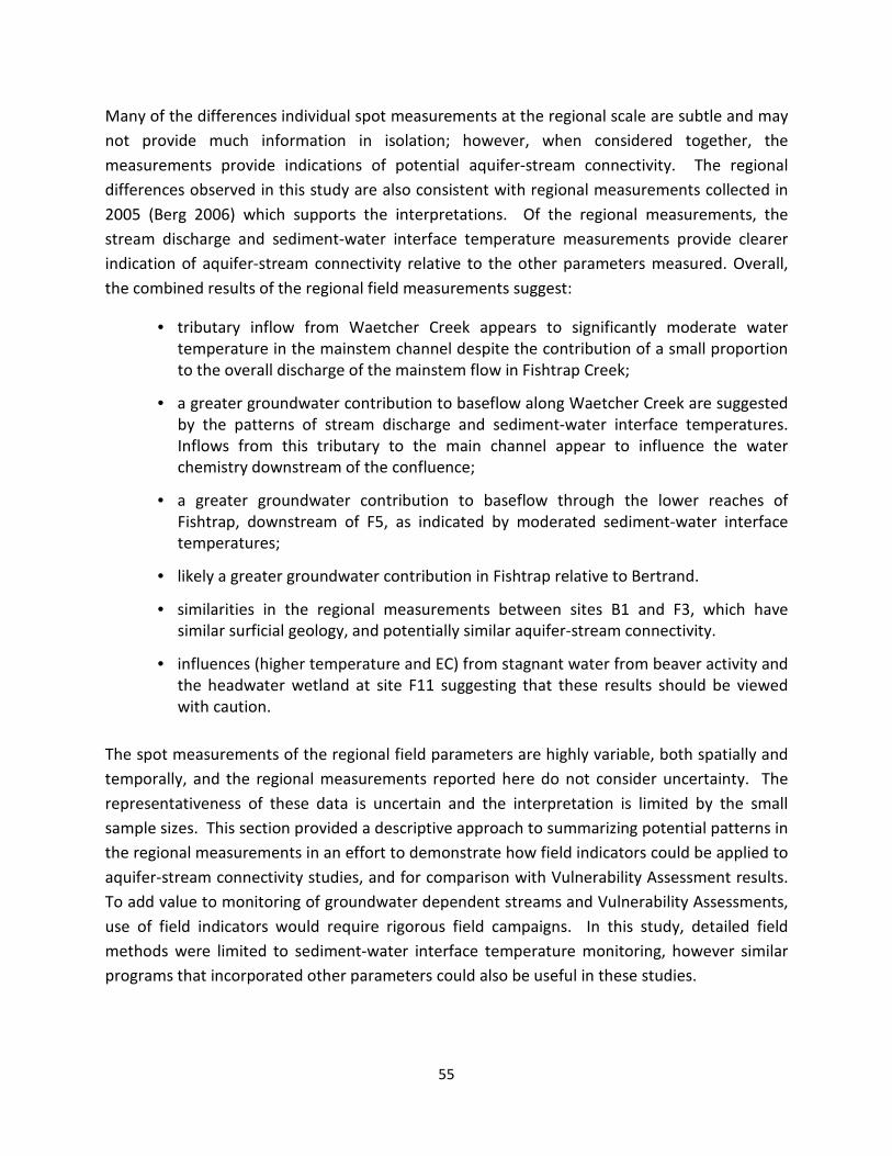
55

Many of the differences individual spot measurements at the regional scale are subtle and may not provide much information in isolation; however, when considered together, the measurements provide indications of potential aquifer-stream connectivity. The regional differences observed in this study are also consistent with regional measurements collected in 2005 (Berg 2006) which supports the interpretations. Of the regional measurements, the stream discharge and sediment-water interface temperature measurements provide clearer indication of aquifer-stream connectivity relative to the other parameters measured. Overall, the combined results of the regional field measurements suggest:

• tributary inflow from Waetcher Creek appears to significantly moderate water temperature in the mainstem channel despite the contribution of a small proportion to the overall discharge of the mainstem flow in Fishtrap Creek;

• a greater groundwater contribution to baseflow along Waetcher Creek are suggested by the patterns of stream discharge and sediment-water interface temperatures. Inflows from this tributary to the main channel appear to influence the water chemistry downstream of the confluence;

• a greater groundwater contribution to baseflow through the lower reaches of Fishtrap, downstream of F5, as indicated by moderated sediment-water interface temperatures;

• likely a greater groundwater contribution in Fishtrap relative to Bertrand.

• similarities in the regional measurements between sites B1 and F3, which have similar surficial geology, and potentially similar aquifer-stream connectivity.

• influences (higher temperature and EC) from stagnant water from beaver activity and the headwater wetland at site F11 suggesting that these results should be viewed with caution.

The spot measurements of the regional field parameters are highly variable, both spatially and temporally, and the regional measurements reported here do not consider uncertainty. The representativeness of these data is uncertain and the interpretation is limited by the small sample sizes. This section provided a descriptive approach to summarizing potential patterns in the regional measurements in an effort to demonstrate how field indicators could be applied to aquifer-stream connectivity studies, and for comparison with Vulnerability Assessment results. To add value to monitoring of groundwater dependent streams and Vulnerability Assessments, use of field indicators would require rigorous field campaigns. In this study, detailed field methods were limited to sediment-water interface temperature monitoring, however similar programs that incorporated other parameters could also be useful in these studies.

56

6.2.8 Comparing Regional Field Measurements to Vulnerability Assessment Results

The Level I and II Assessments for Bertrand and Fishtrap Creeks took a generalized watershed approach for evaluating the vulnerability of the streams. For the Level III Assessment, the Zone Budget results from the numerical model refined the results by considering zones categorized into main channel and ephemeral sections. For example, in Fishtrap watershed, the ephemeral stream zones delineated in Zone Budget were primarily in the upper reaches of the watershed, and the tributaries: Waetcher Creek and the west segments of Enns Brook (Figure 16), corresponding to field locations F8, F9, F12 and F13. The regional field data was included to support the Zone Budget results by identifying stream sections with potentially greater groundwater contributions, both along the sections corresponding to defined zones in Zone Budget, and also within the zone segments. The regional temperature and chemistry data similarly suggest greater groundwater contribution to baseflow along Waetcher Creek and the upper reaches in the west portion of the watershed.

At the watershed scale, both the Level II and Level III Assessments estimated a larger volume of baseflow in Fishtrap Creek relative to Bertrand Creek. The regional field data, primarily the rigorous streambed-water interface temperature monitoring, also show a likely greater groundwater contribution in Fishtrap relative to Bertrand. However, the regional field results suggest greater groundwater contributions to baseflow through the lower reaches of Fishtrap, downstream of F5, and similarities between the temperature and water chemistry between B1 and F3. These areas and patterns of groundwater contribution were not detected in the Zone Budget, and provide an example of how field indicators could be used to refine Vulnerability Assessment for site specific requirements and identify stream segments with higher potential vulnerability.


Regardless of the approach used in a Level III Assessment, there will be uncertainty in the predicted impact. These uncertainties can arise due to a poor conceptual understanding of how the system functions, a lack of information on the properties of the system (e.g. the hydraulic properties), and/or a poor understanding of the stressors themselves (e.g., changes in recharge under future climate change). For these reasons, it is important to recognize sources of uncertainty in a Level III Assessment and convey the implications of uncertainties in a transparent manner.

Changes to recharge can result from changes in land use/land cover, climate variability and climate change. Several studies have been conducted in BC concerning the potential responses of aquifer systems to changes in recharge (e.g., Scibek and Allen, 2006a; Scibek and Allen 2006b; Scibek et al. 2007; Toews and Allen 2009; Allen et al. 2011). Uncertainties in future

57

climate projections, downscaling methods, current recharge estimates and aquifer dynamics complicate the ability to predict how climate change, or indeed climate variability, might influence recharge.

Current best practices for estimating aquifer responses to climate change recommend numerical hydrogeological modeling (Holman et al. 2012). For similar reasons, changes in recharge due to land use/land cover change also would require numerical hydrogeological modeling.

7 Risk Assessment / Risk Management Framework

The results of Level II and Level III Assessments can be integrated into a risk assessment / risk management framework (Figure 27). In addition to assessing stream vulnerability, the consequence of the impacts to the stream must be assessed so as to assess the risk to the stream as summarized below. A full risk assessment in combination with monitoring (using specific indicators for the stream) could be utilized to develop integrated management plans for water quantity planning in aquifer-stream systems. These plans could include measures such as well set-back distances or buffer zones along sensitive streams, and integrated planning for abstraction volumes.

Figure 27. Flow chart for stream vulnerability within a risk assessment framework.

58

7.1 Risk to a Stream

The risk to a stream resulting from a specific hazard is defined in Equation 8, and the components of the risk framework are shown in Figure 28.

Risk (R) = Stream Vulnerability (SV) * Loss (L) (8)

The Level II Assessment results in a rating for Stream Vulnerability. The second component of the risk equation is the Loss (L), which is the consequence of a change to stream flow quantity resulting from stressors in the aquifer system (such as pumping). This loss component can represent a range of impacts, including economic losses from changes in flow conditions, or restoration costs, human health impacts from changes to drinking water sources, and ecological losses. The ecological loss component may arise from loss of ecosystem health, or loss of the valuation assigned to the ecosystem service. For example, a loss of ecosystem health could relate to insufficient flow to sustain fish habitat, as is currently defined for Coho salmon (Oncorhynchus kisutch) under the Sensitive Stream Designation in the Fish Protection Act. The value assigned to this loss component could be based on presence or absence of this loss arising from loss of stream flow. The loss may be related to costs in the mitigation strategies, such as relocation of migrating salmon, loss of water use due to surface water license restrictions, or changes in groundwater use such as relocation of pumping wells outside the boundary of the active zone of the stream.

7.2 Risk Management Example

As an example of risk management, the Zone Budget results for the Fishtrap and Bertrand Watersheds indicated that stream discharge would decrease in both watersheds as result of groundwater pumping, with likely greater decreases in the ephemeral stream sections. These results suggest that the ephemeral stream segments receive greater groundwater contributions on an annual basis, and likely in the summer periods. Figure 28 shows the measured discharge in summer 2009 at various regional sites along with the estimated percent decrease in discharge due to pumping based on the Zone Budget results. The stream discharge was measured while an unknown number of wells were pumped in the watershed. Therefore pumping impacts to the streamflow are likely incorporated in the measurements; however, these discharge values were used in the absence of available non-pumping discharge measurements in order to provide an example how field indicators can be combined with the Level III Assessment for risk management. The ephemeral streams have much lower discharge than the main stem of Fishtrap Creek. The Zone Budget results estimated decreases in overall discharge in the streams as a result of pumping (Figure 28), with the greater impact in the groundwater-dependent ephemeral sections. Given that the regional field data show that the stream temperatures and discharge from the ephemeral reaches influence the downstream

59

stream sections (Figures 22 and 23), it is likely that decreases in baseflow due to pumping will not only reduce the stream flow, but will also result in reduced buffering of high summer stream temperatures. Decreases in stream flow and increases in water temperature can be associated with decreased aquatic habitat suitability, and thus could be quantified as loss of ecosystem health. As shown in Figure 27, the field indicators (here discharge) can be used to monitor the status of the stream and groundwater contributions for management of the risk.

Figure 28. Stream discharge measured regionally in summer 2009 (light blue) with the

percent decrease in summer baseflow estimated in the Zone Budget results (black).

60

8 References

Alexander, M., and D. Caissie. 2003. Variability and comparison of hyporheic water temperatures and seepage fluxes in a small Atlantic salmon stream. Ground Water 41 (1): 72-82.

Allen, D. M., D. C. Mackie, and M. Wei. 2004. Groundwater and climate change: A sensitivity analysis for the grand forks aquifer, southern British Columbia, Canada. Hydrogeology Journal 12(3): 270-90.

Allen, D. M., K. Stahl, P. H. Whitfield, and R. D. Moore. 2014. Trends in groundwater levels in British Columbia. Canadian Water Resources Journal 39 (1): 15-31.

Allen, D. M., P. H. Whitfield, and A. Werner. 2010. Groundwater level response in temperature mountainous terrain: Regime classification, and linkages to climate and streamflow. Hydrological Processes 24(23): 3392-412.

Allen, R. G., L. S. Pereira, D. Raes, and M. Smith. 1998. Crop evapotranspiration - guidelines for computing crop water requirements. Rome: Food and Agriculture Organization of the United Nations, FAO Irrigation and drainage paper 56.

Alley, W. M., T. E. Reilly, and O. L. Franke. 1999. Sustainability of ground-water resources. US Geological Survey, US Geological Survey, Circular 1186

Anderson, M. 2005. Heat as a ground water tracer. Ground Water 43 (6): 951-68.

Angerman, L., S. Krause, and J. Lewanowski. 2012. Application of heat pulse injections for investigating shallow hyporheic flow in a lowland area. Water Resources Research 48: W00P02.

Arnell, N. 2002. Hydrology and global environmental change. Prentice Hall.

Barlow, P. M., and S. A. Leake. 2012. Streamflow depletion by Wells—Understanding and managing the effects of groundwater pumping on streamflow. US Geological Survey, US Geological Survey, Circular 1376

Baxter, C., F. R. Hauer, and W. Woessner. 2003. Measuring groundwater-stream water exchange: New techniques for installing minipiezometers and estimating hydraulic conductivity. Transactions of the American Fisheries Society 132 (3): 493-502.

61

BC Ministry of Environment. 2014 Water protection & sustainability branch: Aquifers. In Government of British Columbia [database online]. 2014 [cited 2014, 08/28 2014]. Available from http://www.env.gov.bc.ca/wsd/plan_protect_sustain/groundwater/aquifers/ (accessed 2014, 08/28).

Becker, M. W., T. Georgian, H. Ambrose, J. Siniscalchi, and K. Fredrick. 2004. Estimating flow and flux of ground water discharge using water temperature and velocity. Journal of Hydrology 296 (1-4): 221-33.

Berandinucci, J., and K. Ronneseth. 2002. Guide to using the BC aquifer classification maps for the protection and management of groundwater. Victoria: British Columbia Ministry of Water, Land and Air Protection.

Berg, M. A. 2006. Stream discharge and hydrochemical variation over the low flow season in the Abbotsford-Sumas aquifer, British Columbia. Bachelor of Science Honors Thesis., Simon Fraser University.

Berg, M. A., and D. M. Allen. 2007. Low flow variability in groundwater-fed streams. Canadian Water Resources Journal 32 (3): 227-45, http://pubs.nrc-cnrc.gc.ca/cwrj/cwrj.html.

Bill 18: Water Sustainability Act, 2014. Third reading, April 29, 2014, 40th Parliament, 2nd Session. Retrieved from: https://www.leg.bc.ca/pages/bclass-legacy.aspx#/content/legacy/web/40th2nd/3rd_read/gov18-3.htm

Bill 25: Fish Protection Act, 1997. First reading, 36th Parliament, 2nd Session. Retrieved from: http://www.env.gov.bc.ca/habitat/fish_protection_act/act/documents/act-theact.html

Boulton, A. 1993. Stream ecology and surface-hyporheic hydrologic exchange: Implications, techniques and limitations. Australian Journal of Marine and Freshwater Research 44 (4): 553-64.

Brewer, S. K. 2013. Groundwater influences on the distribution and abundance of riverine smallmouth bass, Micropterus dolomieu, in pasture landscapes of the midwestern USA. River Research and Applications 29: 269-78.

Briggs, M. A., E. B. Voytek, F. D. Day-Lewis, D. O. Rosenberry, and J. W. Lane. 2013. Understanding water column and streambed thermal refugia for endangered mussels in the Delaware River. Environmental Science and Technology 47 (20): 11423-31.

Brodie, R., S. Baskaran, T. Ransley, and J. Spring. 2009. Seepage meter: Progressing a simple method of directly measuring water flow between surface water and groundwater systems. Australian Journal of Earth Sciences 56 (1): 3-11.

http://www.env.gov.bc.ca/wsd/plan_protect_sustain/groundwater/aquifers/

http://pubs.nrc-cnrc.gc.ca/cwrj/cwrj.html

https://www.leg.bc.ca/pages/bclass-legacy.aspx#/content/legacy/web/40th2nd/3rd_read/gov18-3.htm

https://www.leg.bc.ca/pages/bclass-legacy.aspx#/content/legacy/web/40th2nd/3rd_read/gov18-3.htm

62

Caissie, D. 2006. The thermal regime of rivers: A review. Freshwater Biology 51 (8): 1389-406.

Caissie, D., B. L. Kurylyk, A. St-Hilaire, N. El-Jabi, and T. B. MacQuarrie. 2014. Streambed temperature dynamics and corresponding heat fluxes in small streams experiencing seasonal ice cover. Journal of Hydrology 519 (1441): 1452.

Cardenas, M. 2008. The effect of river bend morphology on flow and timescales of surface water–groundwater exchange across pointbars. Journal of Hydrology 362 (1-2): 134-41.

Carndenas, M. and J. L. Wilson. 2006. The influence of ambient groundwater discharge on exchange zones induced by current–bedform interactions. Journal of Hydrology 331 (1-2): 103-109.

Cey, E. E., D. L. Rudolph, G. W. Parkin, and R. Aravena. 1998. Quantifying groundwater discharge to a small perennial stream in southern Ontario, Canada. Journal of Hydrology 210 (1-4) (SEP): 21-37.

Chesnaux, R., D. M. Allen, and G. Graham. 2007. Assessment of the impact of soil amendment practices on nitrate contamination in the Abbotsford-Sumas aquifer. Environmental Science and Technology 41 (21): 7229-34.

Cohen, S., D. Neilson, and R. Welbourn, eds. 2004. Expanding the dialogue on climate change & water management in the Okanagan Basin, British Columbia. Final report, January 1, 2002 to June 30, 2004. Ottawa, ON: Climate Change Action Fund, Natural Resources Canada.

Conant, B. 2004. Delineating and quantifying ground water discharge zones using streambed temperatures. Ground Water 42 (2): 243-57.

Constantz, J. 2008. Heat as a tracer to determine streambed water exchanges. Water Resources Research 44: W00D10.

———. 1998. Interaction between stream temperature, streamflow, and groundwater exchanges in alpine streams. Water Resources Research 34 (7): 1609-15.

Déry, Stephen J., K. Stahl, R. D. Moore, P. H. Whitfield, B. Menounos, and Jason E. Burford. 2009. Detection of runoff timing changes in pluvial, nival, and glacial rivers of western Canada. Water Resources Research 45 (4).

Environment Canada. Canadian climate normals online, CDCD west CD. 2007 [cited March 9 2009]. Available from http://climate.weatheroffice.ec.gc.ca.proxy.lib.sfu.ca/prods_servs/cdcd_iso_e.html.

http://climate.weatheroffice.ec.gc.ca.proxy.lib.sfu.ca/prods_servs/cdcd_iso_e.html

63

Essaid, H. I., C. M. Zamora, K. A. McCarthy, J. R. Vogel, and J. T. Wilson. 2008. Using heat to characterize streambed water flux variability in four stream reaches. Journal of Environmental Quality 37 (3): 1010-23.

Fleming, Sean W., and Edward J. Quilty. 2006. Aquifer responses to el Niño–Southern oscillation, southwest British Columbia. Ground Water 44 (4): 595-9.

Foster, S., and D. M. Allen. 2015 (in Press). Groundwater – surface water interactions in a mountain-to-coast watershed: Effects of climate change and human stressors. Advances in Meteorology, Special Issue on Hydrological Processes in Changing Climate, Land Use and Cover Change, Article ID 861805 (open access).

Harvey, J. W., and K. E. Bencala. 1993. The effect of streambed topography on surface-subsurface water exchange in mountain catchments. Water Resources Research 29 (1): 89-98.

Hatch, C. E., A. T. Fisher, Revenaugh, J.S., Constantz,J., and C. Ruehl. 2006. Quantifying surface water-groundwater interactions using time series analysis of streambed thermal records: Method development. Water Resources Research 42.

Herrera-Pantoja, M., and K. M. Hiscock. 2008. The effect of climate change on groundwater recharge in Great Britain. Hydrological Processes 22(1): 73-86.

Hess, T. M. 1996. Evapotranspiration estimates for water balance scheduling in the UK. Irrigation News 25: 31-6.

Holman, I. P., D. M. Allen, M. O. Cuthbert, and P. Goderniaux. 2012. Towards best practice for assessing the impacts of climate change on groundwater. Hydrogeology Journal 20 (1): 1-4.

Johnson, S. L. 2003. Stream temperature: Scaling of observations and issues for modelling. Hydrological Processes 17: 497-9.

Johnson, S. L., and J. A. Jones. 2000. Stream temperature responses to forest harvest and debris flows in western Cascades, Oregon. Canadian Journal of Fisheries and Aquatic Sciences 57: 30-9.

Kalbus, E., F. Reinstorf, and M. Schirmer. 2006. Measuring methods for groundwater - surface water interactions: A review. Hydrology and Earth System Sciences 10 (6): 873-87.

64

Krause, S., T. Blume, and N. J. Cassidy. 2012. Investigating patterns and controls of groundwater up-welling in a lowland river by combining fibre-optic distributed temperature sensing with observations of vertical hydraulic gradients. Hydrology and Earth System Sciences 16: 1775-92.

Krause, S., A. Bronstert, and E. Zehe. 2007. Groundwater-surface water interactions in a north German lowland floodplain - implications for the river discharge dynamics and riparian water balance. Journal of Hydrology 347 (3-4): 404-17.

Kreye, R., and M. Wei. 1994. A proposed aquifer classification system for ground water management in British Columbia. Victoria, BC: Ministry of Environment, Lands, and Parks, Water Management Division.

Lowry, C. S., J. F. Walker, R. J. Hunt, and M. P. Anderson. 2007. Indentifying spatial variability of groundwater discharge in a wetland stream using a distributed temperature sensor. Water Resources Research 43: 1-9.

Malcolm, I., C. Soulsby, A. Youngson, and D. Hannah. 2005. Catchment-scale controls on groundwater-surface water interactions in the hyporheic zone: Implications for salmon embryo survival. River Research and Applications 21 (9): 977-89.

Merritt, W. S., Y. Alila, M. Barton, B. Taylor, S. Cohen, and D. Neilson. 2006. Hydrologic response to scenarios of climate change in sub watersheds of the Okanagan Basin, British Columbia. Journal of Hydrology 326: 79-108.

Middleton, M. A. 2016. Aquifer – stream connectivity at various scales; Application of sediment – water interface temperature and vulnerability assessments of groundwater dependent streams. PhD Thesis., Simon Fraser University, Department of Earth Sciences.

Moore, R. D., D. M. Allen, and K. and Stahl. 2007. Climate change and low flows: Influences of groundwater and glaciers. Climate Change Action Fund, Final Report Project A875.

Moore, R. D., D. L. Spittlehouse, and A. Story. 2005. Riparian microclimate and stream temperature response to forest harvest: A review. Journal of the American Water Resources Association 4194): 813-34.

Pike, R. G., K. E. Bennett, T. E. Redding, A. T. Werner, D. L. Spittlehouse, R. D. Moore, T. Q. Murdock, et al. 2010. Climate change effects on watershed processes in British Columbia (chapter 19). In Compendium of forest hydrology and geomorphology in British Columbia. Land Management Handbook 66,., eds. R. G. Pike, T. E. Redding, R. D. Moore, R. D. Winker and K. D. Bladon. Vol. 2 of 2, 699-747. Victoria, BC: B.C. Min. For. Range, For. Sci. Prog.

65

Pruneda, E. B. 2007. Use of stream response functions and Stella software to determine impacts of replacing surface water diversions with groundwater pumping withdrawals on in-stream flows within the Bertrand Creek and Fishtrap Creek watersheds, Washington state, USA. M.Sc. Thesis., Washington State University, Dept. of Civil and Environmental Engineering.

Rau, G. C., M. S. Andersen, A. M. McCallum, H. Roshan, and R. I. Acworth. 2014. Heat as a tracer to quantify water flow in near-surface sediments. Earth-Science Reviews 129: 40-58.

Rosenberry, D. 2008. A seepage meter designed for use in flowing water. Journal of Hydrology 359 (1-2): 118-30.

Rosenberry, D., and J. W. LaBaugh. 2008. Field techniques for estimating water fluxes between surface water and ground water. Reston, Virgina: US Geological Survey, Techniques and methods 4-D2.

Scibek, J. 2005. Modelling the impacts of climate change on groundwater: A comparative study of two unconfined aquifers in Southern British Columbia and Northern Washington State. M.Sc. Thesis., Simon Fraser University, Department of Earth Sciences.

Scibek, J., and D. M. Allen. 2006a. Comparing the responses of two high permeability, unconfined aquifers to predicted climate change. Global and Planetary Change 50: 50-62.

———. 2006b. Modeled impacts of predicted climate change on recharge and groundwater levels. Water Resources Research 42.

Scibek, J., and D. M. Allen. 2005. Numerical groundwater flow model of the Abbotsford-Sumas aquifer, Central Fraser Lowland of BC, Canada, and Washington State, US. Prepared for Environment Canada.

Scibek, J., D. M. Allen, A. Cannon, and P. H. Whitfield. 2007b. Groundwater-surface water interaction under scenarios of climate change using a high-resolution transient groundwater model. Journal of Hydrology 333: 162-81.

Silliman, S. E., and D. F. Booth. 1993. Analysis of time-series measurements of sediment temperature for identification of gaining vs. losing portions of Juday Creek, Indiana. Journal of Hydrology 146 (1-4): 131-48.

Sophocleous, M. 2002. Interactions between groundwater and surface water: The state of the science. Hydrogeology Journal 10 (1): 52-67.

66

Stonestrom, D. A., and J. Constantz, eds. 2003. Heat as a tool for studying the movement of ground water near streams: U.S. Geological Survey Circular 1260, 96 p. http://pubs.water.usgs.gov/circ1260: USGS.

Toews, M. W., and D. M. Allen. 2009. Simulated response of groundwater to predicted recharge in a semi-arid region using A scenario of modelled climate change. Environmental Research Letters 4.

Washington State Department of Ecology. Solrad.v. 1.2: A solar position and radiation calculator for Microsoft Excel/VBA. State of Washington, 2014 [cited 04/15 2014]. Available from http://www.ecy.wa.gov/programs/eap/models.html (accessed 2014/04/15).

Wei, M., D. M. Allen, A. Kohut, S. Grasby, K. Ronneseth, and B. Turner. 2009. Understanding the types of aquifers in the Canadian Cordillera hydrogeologic region to better manage and protect groundwater. Streamline Water Management Bulletin 13(1): 10-8.

Winter, T. C., J. W. Harvey, O. L. Franke, and W. M. Alley. 1998. Groundwater and surface water – a single resource. US Geological Survey, US Geological Survey, Circular 1139.

http://pubs.water.usgs.gov/circ1260

http://www.ecy.wa.gov/programs/eap/models.html

67

Appendix A. Level III Assessment - Comparing Impacts for Non-Pumping and Pumping for Fishtrap and Bertrand Creek Watersheds

Non-Pumping Impacts to the Watershed Zones

The Zone Budget results for the non-pumping conditions for Fishtrap and Bertrand Creek watersheds are shown in Figures A1 and A2, respectively. The results are divided into the main Zone Budget zones: the watershed zone, the main-stem stream zones, and the ephemeral stream zones. The results show the main water inputs to the watershed zones is recharge with some exchange between zones. The exchanges between the zones for each watershed are dominated by exchange between the watershed zones (zones 2 and 9) and the main aquifer zone (zone 1), rather than with the main stem and ephemeral zones. Water leaving the watershed zones, goes partially into storage and partially as zone transfers (discussed in more detail below). The Zone Budget results for the stream segments (Figures A1 and A2) indicate that water exchange from other zones, primarily from the broader watershed zone, is the main input of water, and water leaves the stream main stem zone via the river and drain cells which comprise these two zones. For the ephemeral stream segments, the drain cells are the primary outflow zones, which is to be expected given that drains are the boundary condition for most of the ephemeral reaches.

The gain in storage over the year is an interesting outcome and a consequence of the initial head distribution (steady-state heads) for the transient simulation. An examination of the heads time series suggests that heads gradually increase over the simulation time period, consistent with water being added to storage. Upon closer examination of the detailed water balance, water is made available to a zone from storage or is lost from the zone to storage. In Fishtrap and Bertrand watersheds, more water is supplied to the zone from storage during the summer months, and in the winter more water goes into storage. This is an expected outcome. Over the long term, roughly the same amount of water should go into and out of storage on an annual basis. However, for this single simulation year, both watershed zones lose more water to storage (Figures A1 and A2). Thus, the annual water budget is not reflecting conditions that might be expected over the long term. The model is not in dynamic equilibrium for this single year simulation. Multiple years could be run to achieve a better dynamic equilibrium, and the first few years of output removed for analysis of outputs. This is referred to as model spin up. The water balance would then be examined over the latter portion of the simulation period. Consequently, the overall annual water balance results should be viewed with caution. Over the longer term, the amount of water entering storage should equal the amount leaving storage. This suggests that of the amount of recharge added to the watershed, most of the water will exit to other zones, resulting in the green bars (zone transfer out of the watershed in Figures A1 and A2) comprising the only outflow component. Notwithstanding the storage problem, changes in the water balance results between the pumping and non-pumping conditions are likely fairly representative. If water does not come from storage to supply pumping, then water would come from elsewhere. Therefore, the results are conservative.

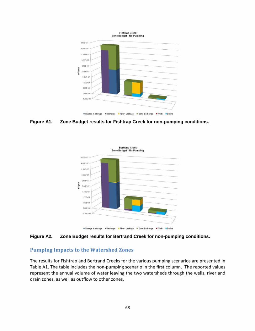
68

Figure A1. Zone Budget results for Fishtrap Creek for non-pumping conditions.

Figure A2. Zone Budget results for Bertrand Creek for non-pumping conditions.

Pumping Impacts to the Watershed Zones

The results for Fishtrap and Bertrand Creeks for the various pumping scenarios are presented in Table A1. The table includes the non-pumping scenario in the first column. The reported values represent the annual volume of water leaving the two watersheds through the wells, river and drain zones, as well as outflow to other zones.

69

Table A1. Zone Budget results showing the annual water volume out of the Fishtrap and Bertrand Creek watersheds zones.

No Pumping

(m3/yr)

Pumping Single

Watershed (m3/yr)

Pumping Other

Watershed (m3/yr)

Pumping Both

Watersheds (m3/yr)

Pumping All Model Wells

(m3/yr) Fishtrap Creek 3.46E+07 4.33E+07 1.12E+07 2.69E+07 2.69E+07 Bertrand Creek 3.31E+07 3.56E-07 2.83E+07 3.58E+07 3.58E+07

The pumping scenarios show that for each stream, the strongest influence is the result of pumping within the respective watershed, manifested by an increase in the water volume out of the watershed (Table A1; Figures A3 and A7). There is an apparent decrease in the volume of water out of each watershed through the river, drain, wells, and to other zones during the pumping scenarios when wells in other model areas are activated. This is due diversion of available water to the pumped wells, and a subsequent decrease in water volume into the individual watersheds.

Cumulative impacts from pumping outside the watershed result in a decrease in the water volume out of the watershed (Table A1) and the volumes are the same if the pumping is occurring in the two watersheds (Figures A5 and A6) or aquifer-wide (Figures A9 and A10). Therefore, the watershed boundary (in this study) provides an appropriate boundary to monitor pumping when there is pumping across a wider area.

When pumping occurs only in the adjacent watershed (Figure A4 and A8), there is a larger apparent decrease in the water volume out of the watershed. This is because available water in the model is being drawn to the adjacent watershed, and there is no pumping in the specified watershed drawing water from other zones. There is the potential that pumping in each watershed, when isolated, will have influence on an area larger than the watershed boundary. The impacts to adjacent watersheds can be direct as well, as seen in the Bertrand watershed, where a minor volume of water from the ephemeral stream segments is lost to wells when pumping is activated in the Fishtrap Creek watershed (Figure A8). These ephemeral stream reaches are higher order segments of the stream, which are closer to the boundary of the watershed, and therefore some segments are located closer to the pumping wells adjoining watershed. Consequently, pumping in adjacent watersheds only can have the combined effect of intercepting water that would have entered the watershed, and directly drawing water away. For the scenario with all of the pumping wells across the model area activated, the results indicate decreases in total water volume out of each watershed on the order of approximately 105 m3/year, relative to the non-pumping scenario.

70

Figure A3. Zone Budget results for Fishtrap Creek for wells pumping only in the

Fishtrap Creek watershed.

Figure A4. Zone Budget results for Fishtrap Creek for wells pumping only in the

adjacent Bertrand Creek watershed.

71

Figure A5. Zone Budget results for Fishtrap Creek for wells pumping in both Fishtrap

and Bertrand Creek watersheds.

Figure A6. Zone Budget results for Fishtrap Creek for all wells pumping throughout

the model domain.

72

Figure A7. Zone Budget results for Bertrand Creek for wells pumping only in the

Bertrand Creek watershed.

Figure A8. Zone Budget results for Bertrand Creek for wells pumping only in the

adjacent Fishtrap Creek watershed.

73

Figure A9. Zone Budget results for Bertrand Creek for wells pumping in both Fishtrap

and Bertrand Creek watersheds.

Figure A10. Zone Budget results for Bertrand Creek for all wells pumping throughout

the model domain.

Vulnerability Assessment for Groundwater Dependent...

Documents

Transcript of Vulnerability Assessment for Groundwater Dependent...