Vtusolutionvtusolution.in/uploads/9/9/9/3/99939970/mechanical_vibrations[10me... · Resonance is...
167
vtusolution.in Introduction: When an elastic body such as, a spring, a beam and a shaft are displaced from the equilibrium position by the application of external forces, and then released, they execute a vibratory motion, due to the elastic or strain energy present in the body. When the body reaches the equilibrium position, the whole of the elastic or stain energy is converted into kinetic energy due to which the body continues to move in the opposite direction. The entire KE is again converted into strain energy due to which the body again returns to the equilibrium position. Hence the vibratory motion is repeated indefinitely. Oscillatory motion is any pattern of motion where the system under observation moves back and forth across some equilibrium position, but dose not necessarily have any particular repeating pattern. Periodic motion is a specific form of oscillatory motion where the motion pattern repeats itself with a uniform time interval. This uniform time interval is referred to as the period and has units of seconds per cycle. The reciprocal of the period is referred to as the frequency and has units of cycles per second. This unit of combination has been given a special unit symbol and is referred to as Hertz (Hz) Harmonic motion is a specific form of periodic motion where the motion pattern can be describe by either a sine or cosine. This motion is also sometimes referred to as simple harmonic motion. Because the sine or cosine technically used angles in radians, the frequency term expressed in the units radians per seconds (rad/sec). This is sometimes referred to as the circular frequency. The relationship between the frequency in Hz (cps) and the frequency in rad/sec is simply the relationship. 2π rad/sec. Natural frequency is the frequency at which an undamped system will tend to oscillate due to initial conditions in the absence of any external excitation. Because there is no damping, the system will oscillate indefinitely. Damped natural frequency is frequency that a damped system will tend to oscillate due to initial conditions in the absence of any external excitation. Because there is damping in the system, the system response will eventually decay to rest. Resonance is the condition of having an external excitation at the natural frequency of the system. In general, this is undesirable, potentially producing extremely large system response. Degrees of freedom: The numbers of degrees of freedom that a body possesses are those necessary to completely define its position and orientation in space. This is useful in several fields of study such as robotics and vibrations. Consider a spherical object that can only be positioned somewhere on the x axis. UNIT - 1 VIBRATIONS Mechanical Vibrations[10ME72] Dept. Of ME, ACE 1 Vtusolution.in Vtusolution.in
Transcript of Vtusolutionvtusolution.in/uploads/9/9/9/3/99939970/mechanical_vibrations[10me... · Resonance is...

vtuso
lution
.in
06ME 64 - Mechanical Vibrations, Dr.T.V.Givindaraju Introduction 1
Visvesvaraya Technological University
E-notes
Dr. .V. Govindaraju
Principal, Shirdi Sai Engineering College, Bangalore
06ME 64 - MECHANICAL VIBRATIONS UNIT - 1
Introduction: When an elastic body such as, a spring, a beam and a shaft are displaced from the
equilibrium position by the application of external forces, and then released, they execute a vibratory
motion, due to the elastic or strain energy present in the body. When the body reaches the
equilibrium position, the whole of the elastic or stain energy is converted into kinetic energy due to
which the body continues to move in the opposite direction. The entire KE is again converted into
strain energy due to which the body again returns to the equilibrium position. Hence the vibratory
motion is repeated indefinitely.
Oscillatory motion is any pattern of motion where the system under observation moves back and
forth across some equilibrium position, but dose not necessarily have any particular repeating
pattern.
Periodic motion is a specific form of oscillatory motion where the motion pattern repeats itself with a
uniform time interval. This uniform time interval is referred to as the period and has units of seconds
per cycle. The reciprocal of the period is referred to as the frequency and has units of cycles per
second. This unit of combination has been given a special unit symbol and is referred to as Hertz
(Hz)
Harmonic motion is a specific form of periodic motion where the motion pattern can be describe by
either a sine or cosine. This motion is also sometimes referred to as simple harmonic motion.
Because the sine or cosine technically used angles in radians, the frequency term expressed in the
units radians per seconds (rad/sec). This is sometimes referred to as the circular frequency. The
relationship between the frequency in Hz (cps) and the frequency in rad/sec is simply the
relationship. 2π rad/sec.
Natural frequency is the frequency at which an undamped system will tend to oscillate due to initial
conditions in the absence of any external excitation. Because there is no damping, the system will
oscillate indefinitely.
Damped natural frequency is frequency that a damped system will tend to oscillate due to initial
conditions in the absence of any external excitation. Because there is damping in the system, the
system response will eventually decay to rest.
Resonance is the condition of having an external excitation at the natural frequency of the system. In
general, this is undesirable, potentially producing extremely large system response.
Degrees of freedom: The numbers of degrees of freedom
that a body possesses are those necessary to completely
define its position and orientation in space. This is useful in
several fields of study such as robotics and vibrations.
Consider a spherical object that can only be positioned
somewhere on the x axis.
UNIT - 1
VIBRATIONS
Mechanical Vibrations[10ME72]
Dept. Of ME, ACE1
Vtusolution.in
Vtusolution.in

vtuso
lution
.in
06ME 64 - Mechanical Vibrations, Dr.T.V.Givindaraju Introduction 2
This needs only one dimension, ‘x’ to define the position to the centre of gravity so it has one degree
of freedom. If the object was a cylinder, we also need an angle ‘θ’ to define the orientation so it has
two degrees of freedom.
Now consider a sphere that can be positioned in
Cartesian coordinates anywhere on the z plane. This
needs two coordinates ‘x’ and ‘y’ to define the
position of the centre of gravity so it has two
degrees of freedom. A cylinder, however, needs the
angle ‘θ’ also to define its orientation in that plane
so it has three degrees of freedom.
In order to completely specify the position and
orientation of a cylinder in Cartesian space, we
would need three coordinates x, y and z and three
angles relative to each angle. This makes six
degrees of freedom. A rigid body in space has
(x,y,z,θx θy θz).
In the study of free vibrations, we will be
constrained to one degree of freedom.
Types of Vibrations: Free or natural vibrations: A free vibration is one that occurs naturally with no energy being added
to the vibrating system. The vibration is started by some input of energy but the vibrations die away
with time as the energy is dissipated. In each case, when the body is moved away from the rest
position, there is a natural force that tries to return it to its rest position. Free or natural vibrations
occur in an elastic system when only the internal restoring forces of the system act upon a body.
Since these forces are proportional to the displacement of the body from the equilibrium position, the
acceleration of the body is also proportional to the displacement and is always directed towards the
equilibrium position, so that the body moves with SHM.
Figure 1. Examples of vibrations with single degree of freedom.
Note that the mass on the spring could be made to swing like a pendulum as well as bouncing up and
down and this would be a vibration with two degrees of freedom. The number of degrees of freedom
of the system is the number of different modes of vibration which the system may posses.
Mechanical Vibrations [10ME72]
Dept. Of ME, ACE 2
Vtusolution.in
Vtusolution.in
vtuso
lution
.in
06ME 64 - Mechanical Vibrations, Dr.T.V.Givindaraju Introduction
3
The motion that all these examples perform is called SIMPLE HARMONIC MOTION (S.H.M.).
This motion is characterized by the fact that when the displacement is plotted against time, the
resulting graph is basically sinusoidal. Displacement can be linear (e.g. the distance moved by the
mass on the spring) or angular (e.g. the angle moved by the simple pendulum). Although we are
studying natural vibrations, it will help us understand S.H.M. if we study a forced vibration
produced by a mechanism such as the Scotch Yoke.
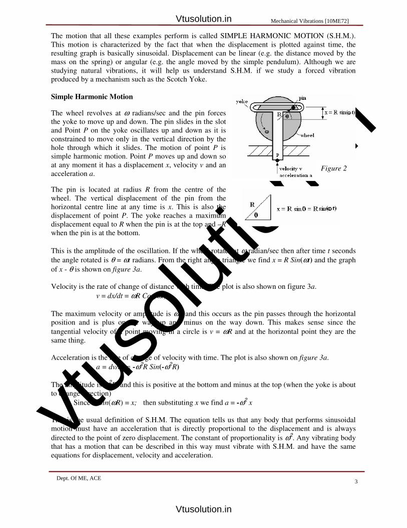
Simple Harmonic Motion
The wheel revolves at ω radians/sec and the pin forces
the yoke to move up and down. The pin slides in the slot
and Point P on the yoke oscillates up and down as it is
constrained to move only in the vertical direction by the
hole through which it slides. The motion of point P is
simple harmonic motion. Point P moves up and down so
at any moment it has a displacement x, velocity v and an
acceleration a.
The pin is located at radius R from the centre of the
wheel. The vertical displacement of the pin from the
horizontal centre line at any time is x. This is also the
displacement of point P. The yoke reaches a maximum
displacement equal to R when the pin is at the top and –R
when the pin is at the bottom.
This is the amplitude of the oscillation. If the wheel rotates at ω radian/sec then after time t seconds
the angle rotated is θ = ωt radians. From the right angle triangle we find x = R Sin(ωt) and the graph
of x - θ is shown on figure 3a.
Velocity is the rate of change of distance with time. The plot is also shown on figure 3a.
v = dx/dt = ωR Cos(ωt).
The maximum velocity or amplitude is ωR and this occurs as the pin passes through the horizontal
position and is plus on the way up and minus on the way down. This makes sense since the
tangential velocity of a point moving in a circle is v = ωR and at the horizontal point they are the
same thing.
Acceleration is the rate of change of velocity with time. The plot is also shown on figure 3a.
a = dv/dt = -ω2R Sin(-ω2
R)
The amplitude is ω2R and this is positive at the bottom and minus at the top (when the yoke is about
to change direction)
Since R Sin(ωR) = x; then substituting x we find a = -ω2 x
This is the usual definition of S.H.M. The equation tells us that any body that performs sinusoidal
motion must have an acceleration that is directly proportional to the displacement and is always
directed to the point of zero displacement. The constant of proportionality is ω2. Any vibrating body
that has a motion that can be described in this way must vibrate with S.H.M. and have the same
equations for displacement, velocity and acceleration.
Figure 2
Mechanical Vibrations [10ME72]
Dept. Of ME, ACE3
Vtusolution.in
Vtusolution.in

vtuso
lution
.in
06ME 64 - Mechanical Vibrations, Dr.T.V.Givindaraju Introduction
4
FIGURE 3a FIGURE 3b
Angular Frequency, Frequency and Periodic time
ω is the angular velocity of the wheel but in any vibration such as the mass on the spring, it is called
the angular frequency as no physical wheel exists.
The frequency of the wheel in revolutions/second is equivalent to the frequency of the vibration. If
the wheel rotates at 2 rev/s the time of one revolution is ½ seconds. If the wheel rotates at 5 rev/s the
time of one revolution is 1/5 second. If it rotates at f rev/s the time of one revolution is
1/f. This
formula is important and gives the periodic time.
Periodic Time T = time needed to perform one cycle.
f is the frequency or number of cycles per second.
It follows that: T = 1/f and f =
1/T
Each cycle of an oscillation is equivalent to one rotation of the wheel and 1 revolution is an angle of
2π radians.
When θ = 2π and t = T.
It follows that since θ = ωt; then 2π = ωT
Rearrange and θ = 2π
/T. Substituting T = 1/f, then ω =2πf
Mechanical Vibrations [10ME72]
4Dept. Of ME, ACE
Vtusolution.in
Vtusolution.in

vtuso
lution
.in
06ME 64 - Mechanical Vibrations, Dr.T.V.Givindaraju Introduction
5
Equations of S.H.M.
Consider the three equations derived earlier.
Displacement x = R Sin(ωt).
Velocity v = dx/dt = ωR Cos(ωt) and Acceleration a = dv/dt = -ω2R Sin(ωt)
The plots of x, v and a against angle θ are shown on figure 3a. In the analysis so far made, we
measured angle θ from the horizontal position and arbitrarily decided that the time was zero at this
point.
Suppose we start the timing after the angle has reached a value of φ from this point. In these cases, φ is called the phase angle. The resulting equations for displacement, velocity and acceleration are then
as follows.
Displacement x = R Sin(ωt + φ).
Velocity v = dx/dt = ωR Cos(ωt + φ).
Acceleration a = dv/dt = -ω2R Sin((ωt + φ).
The plots of x, v and a are the same but the vertical axis is displaced by φ as shown on figure 3b. A
point to note on figure 3a and 3b is that the velocity graph is shifted ¼ cycle (90o) to the left and the
acceleration graph is shifted a further ¼ cycle making it ½ cycle out of phase with x.
Forced vibrations: When the body vibrates under the influence of external force, then the body is
said to be under forced vibrations. The external force, applied to the body is a periodic disturbing
force created by unbalance. The vibrations have the same frequency as the applied force.
(Note: When the frequency of external force is same as that of the natural vibrations, resonance
takes place)
Damped vibrations: When there is a reduction in amplitude over every cycle of vibration, the motion
is said to be damped vibration. This is due to the fact that a certain amount of energy possessed by
the vibrating system is always dissipated in overcoming frictional resistance to the motion.
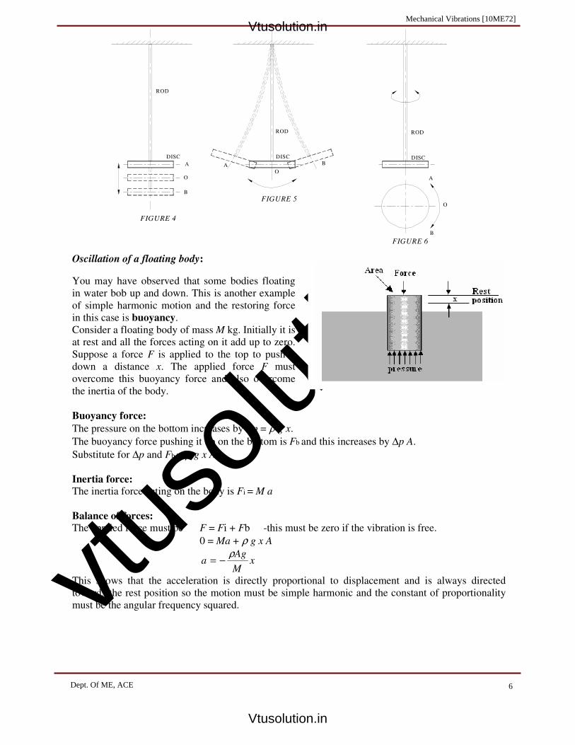
Types of free vibrations:
Linear / Longitudinal vibrations: When the disc is displaced vertically downwards by an external
force and released as shown in the figure 4, all the particles of the rod and disc move parallel to the
axis of shaft. The rod is elongated and shortened alternately and thus the tensile and compressive
stresses are induced alternately in the rod. The vibration occurs is know as Linear/Longitudinal
vibrations.
Transverse vibrations: When the rod is displaced in the transverse direction by an external force and
released as shown in the figure 5, all the particles of rod and disc move approximately perpendicular
to the axis of the rod. The shaft is straight and bends alternately inducing bending stresses in the rod.
The vibration occurs is know as transverse vibrations.
Torsional vibrations: When the rod is twisted about its axis by an external force and released as
shown in the figure 6, all the particles of the rod and disc move in a circle about the axis of the rod.
The rod is subjected to twist and torsional shear stress is induced. The vibration occurs is known as
torsional vibrations.
Mechanical Vibrations [10ME72]
5Dept. Of ME, ACE
Vtusolution.in
Vtusolution.in
vtuso
lution
.in
06ME 64 - Mechanical Vibrations, Dr.T.V.Givindaraju Introduction
6
A
O
B
O
BA
DISC
ROD
DISC
ROD
B
O
A
ROD
DISC
FIGURE 4
FIGURE 5
FIGURE 6
Oscillation of a floating body:
You may have observed that some bodies floating
in water bob up and down. This is another example
of simple harmonic motion and the restoring force
in this case is buoyancy.
Consider a floating body of mass M kg. Initially it is
at rest and all the forces acting on it add up to zero.
Suppose a force F is applied to the top to push it
down a distance x. The applied force F must
overcome this buoyancy force and also overcome
the inertia of the body.
Buoyancy force:
The pressure on the bottom increases by ∆p = ρ g x.
The buoyancy force pushing it up on the bottom is Fb and this increases by ∆p A.
Substitute for ∆p and Fb = ρ g x A
Inertia force:
The inertia force acting on the body is Fi = M a
Balance of forces:
The applied force must be F = Fi + Fb -this must be zero if the vibration is free.
0 = Ma + ρ g x A
xM
Aga
ρ−=
This shows that the acceleration is directly proportional to displacement and is always directed
towards the rest position so the motion must be simple harmonic and the constant of proportionality
must be the angular frequency squared.
Mechanical Vibrations [10ME72]
Dept. Of ME, ACE 6
Vtusolution.in
Vtusolution.in

vtuso
lution
.in
06ME 64 - Mechanical Vibrations, Dr.T.V.Givindaraju Introduction
7
M
Agf
M
Ag
M
Ag
n
ρ
ππ
ω
ρω
ρω
2
1
2
2
==
=
=
Example: A cylindrical rod is 80 mm diameter and has a mass of 5 kg. It floats vertically in water of
density 1036 kg/m3. Calculate the frequency at which it bobs up and down. (Ans. 0.508 Hz)
Principal of super position: The principal of super position means that, when TWO or more
waves meet, the wave can be added or subtracted.
Two waveforms combine in a manner, which simply adds their
respective Amplitudes linearly at every point in time. Thus, a
complex SPECTRUM can be built by mixing together different
Waves of various amplitudes.
The principle of superposition may be applied to waves whenever
two (or more) waves traveling through the same medium at the
same time. The waves pass through each other without being
disturbed. The net displacement of the medium at any point in
space or time, is simply the sum of the individual wave
dispacements.
General equation of physical systems is:
)(tFkxxcxm =++ &&& - This equation is for a
linear system, the inertia, damping and spring force are linear
function xandxx &&& , respectively. This is not true case of non-
linear systems.
)()()( tFxfxxm =++ &&& φ - Damping and spring
force are not linear functions of xandx&
Mathematically for linear systems, if 1x is a solution of;
)(1 tFkxxcxm =++ &&&
and 2x is a solution of;
)(2 tFkxxcxm =++ &&&
then )( 21 xx + is a solution of;
)()( 21 tFtFkxxcxm +=++ &&&
Law of superposition does not hold good for non-linear systems.
If more than one wave is traveling through the medium: The resulting net wave is given by the
Superposition Principle given by the sum of the individual waveforms”
Mechanical Vibrations[10ME72]
7Dept. Of ME, ACE
Vtusolution.in
Vtusolution.in

vtuso
lution
.in
06ME 64 - Mechanical Vibrations, Dr.T.V.Givindaraju Introduction
8
Beats: When two harmonic motions occur with the same amplitude ‘A’ at different frequency is
added together a phenomenon called "beating" occurs.
The resulting motion is:
( ) ( ) ( )[ ]tftfAyyy 2121 2cos2cos ππ +=+=
with trigonometric manipulation, the above
equation can be written as:
tff
tff
Ay2
2cos2
2cos2 2121 +×
−= ππ
The resultant waveform can be thought of as a wave with frequency fave = (f1 + f2)/2 which is
constrained by an envelope with a frequency of fb = |f1 - f2|. The envelope frequency is called the beat
frequency. The reason for the name is apparent if you listen to the phenomenon using sound waves.
(Beats are often used to tune instruments. The desired frequency is compared to the frequency of the instrument. If a beat
frequency is heard the instrument is "out of tune". The higher the beat frequency the more "out of tune" the instrument
is.)
Fourier series: decomposes any periodic function or periodic signal into the sum of a
(possibly infinite) set of simple oscillating functions, namely sines and cosines (or complex
exponentials).
Fourier series were introduced by Joseph Fourier (1768–1830) for the purpose of solving the
heat equation in a metal plate.
The Fourier series has many such applications in electrical engineering, vibration analysis,
acoustics, optics, signal processing, image processing, quantum mechanics, thin-walled shell
theory,etc.
( )tfAy 11 2cos π=
( )tfAy 22 2cos π=
Mechanical Vibrations [10ME72]
8Dept. Of ME, ACE
Vtusolution.in
Vtusolution.in
vtuso
lution
.in
06ME 64 - Mechanical Vibrations, Dr.T.V.Givindaraju Introduction
9
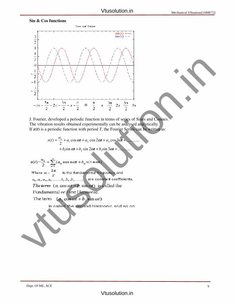
Sin & Cos functions
J. Fourier, developed a periodic function in terms of series of Sines and Cosines.
The vibration results obtained experimentally can be analysed analytically.
If x(t) is a periodic function with period T, the Fourier Series can be written as:
............3sin2sinsin
............3cos2coscos2
)(
321
321
++++
++++=
tbtbtb
tatataa
tx o
ωωω
ωωω
Mechanical Vibrations[10ME72]
9Dept. Of ME, ACE
Vtusolution.in
Vtusolution.in
vtuso
lution
.in
06ME 64 - Mechanical Vibrations, Dr.T.V.Givindaraju Introduction
10
Refer PPT – for more Problems
( )( )
smm
Cos
tCosAvVelocity
/999
963.15020
=
××=
+== φωω
( )
( )2
2
2
/1712
963.15020
smm
Sin
tSinAaonAccelerati
−=
××−=
+−== φωω
Mechanical Vibrations [10ME72]
10Dept. Of ME, ACE
Vtusolution.in
Vtusolution.in

vtuso
lution
.in
06ME 64 - Mechanical Vibrations, Dr.T.V.Givindaraju Undamped Free Vibrations
1
δx
m
W
W=kδ
Unstrained postion
kx
m x
m O
x
k(δ+x)
mg
m
k= Stiffness spring
FIGURE 7
Visvesvaraya Technological University
E-notes
Dr. .V. Govindaraju
Principal, Shirdi Sai Engineering College, Bangalore
06ME 64 - MECHANICAL VIBRATIONS UNIT - 2
Undamped Free Vibrationis:
NATURAL FREQUENCY OF FREE LONGITUDINAL VIBRATION
Equilibrium Method: Consider a body of mass ‘m’ suspended from a spring of negligible mass as
shown in the figure 4.
Let m = Mass of the body
W = Weight of the body = mg
K = Stiffness of the spring
δ = Static deflection of the spring due to ‘W’
By applying an external force, assume the body
is displaced vertically by a distance ‘x’, from the
equilibrium position. On the release of external
force, the unbalanced forces and acceleration
imparted to the body are related by Newton
Second Law of motion.
∴ The restoring force = F = - k × x (-ve sign indicates, the restoring force ‘k.x’ is
opposite to the direction of the displacement ‘x’)
By Newton’s Law; F = m × a
2
2
dt
xdmxkF =−=∴
∴ The differential equation of motion, if a body of mass ‘m’ is acted upon by a restoring force ‘k’
per unit displacement from the equilibrium position is;
SHMrepresentsequationThisxm
k
dt
xd−=+ 0
2
2
SHMform
kx
dt
xd−==+ 22
2
2
0 ωω
The natural period of vibration is Seck
mT π
ω
π2
2==
The natural frequency of vibration is sec/2
1cycles
m
kf n
π=
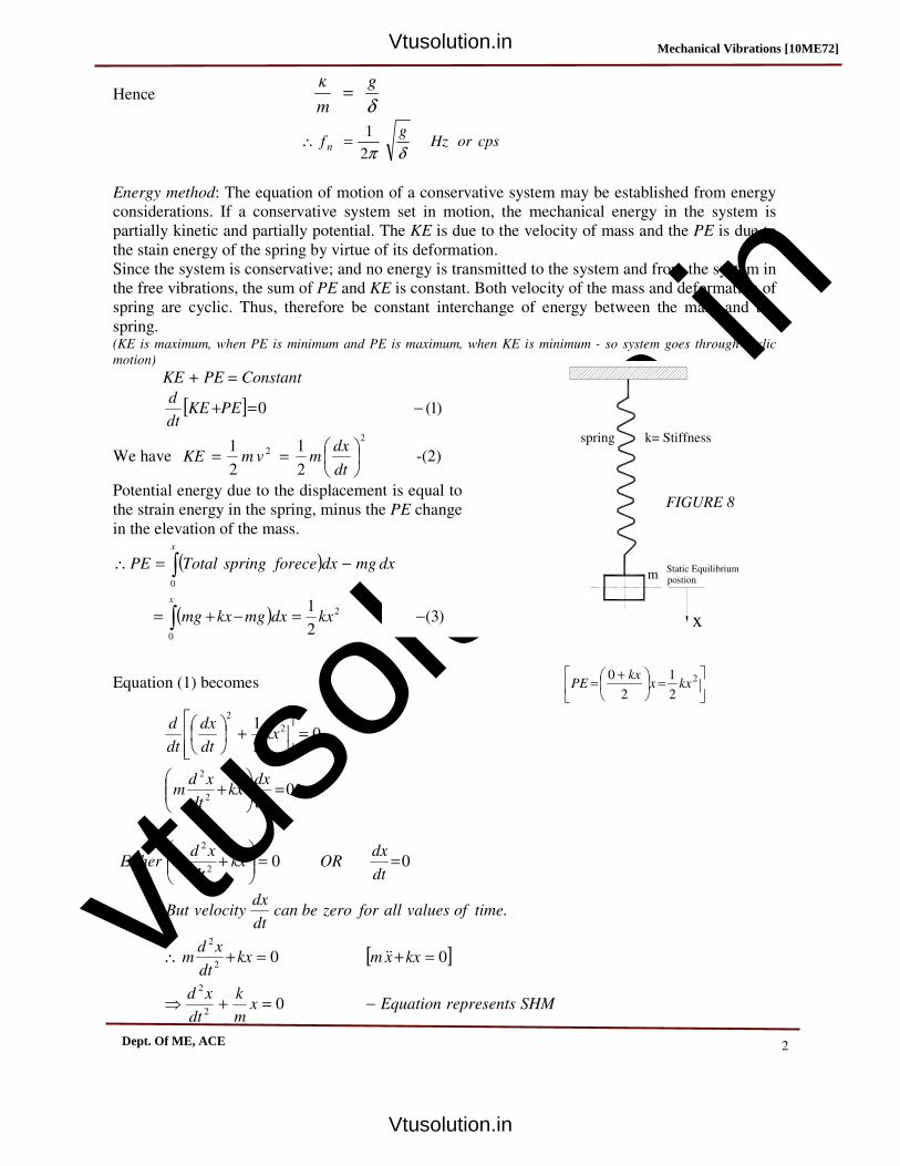
From the figure 7; when the spring is strained by an amount of ‘δ’ due to the weight W = mg
δ k = mg
UNIT 2
UNDAMPED FREE VIBRATIONS
Mechanical Vibrations [10ME72]
Dept. Of ME, ACE
Vtusolution.in
Vtusolution.in
vtuso
lution
.in
06ME 64 - Mechanical Vibrations, Dr.T.V.Givindaraju Undamped Free Vibrations
2
Static Equilibrium
postion
spring
x
m
k= Stiffness
FIGURE 8
Hence δ
g
m
k=
cpsorHzg
f nδπ2
1=∴
Energy method: The equation of motion of a conservative system may be established from energy
considerations. If a conservative system set in motion, the mechanical energy in the system is
partially kinetic and partially potential. The KE is due to the velocity of mass and the PE is due to
the stain energy of the spring by virtue of its deformation.
Since the system is conservative; and no energy is transmitted to the system and from the system in
the free vibrations, the sum of PE and KE is constant. Both velocity of the mass and deformation of
spring are cyclic. Thus, therefore be constant interchange of energy between the mass and the
spring. (KE is maximum, when PE is minimum and PE is maximum, when KE is minimum - so system goes through cyclic
motion)
KE + PE = Constant
[ ] )1(0 −=+PEKEdt
d
We have
2
2
2
1
2
1
==
dt
dxmvmKE -(2)
Potential energy due to the displacement is equal to
the strain energy in the spring, minus the PE change
in the elevation of the mass.
( )
( ) )3(2
1 2
0
0
−=−+=
−=∴
∫
∫
kxdxmgkxmg
dxmgdxforecespringTotalPE
x
x
Equation (1) becomes
=
+= 2
2
1
2
0kxx
kxPE
0
02
1
2
2
2
2
=
+
=
+
dt
dxkx
dt
xdm
kxdt
dx
dt
d
002
2
==
+
dt
dxORkx
dt
xdmEither
[ ]
SHMrepresentsEquationxm
k
dt
xd
kxxmkxdt
xdm
timeofvaluesallforzerobecandt
dxvelocityBut
−=+⇒
=+=+∴
0
00
.
2
2
2
2
&&
Mechanical Vibrations [10ME72]
Dept. Of ME, ACE
Vtusolution.in
Vtusolution.in

vtuso
lution
.in
06ME 64 - Mechanical Vibrations, Dr.T.V.Givindaraju Undamped Free Vibrations
3
sec/2
1
sec2
cyclesm
kfvibrationoffrequencyNatural
andk
mTperiodTime
nπ
π
==
==∴
(The natural frequency is inherent in the system. It is the function of the system parameters 'k' and 'm' and it is
independent of the amplitude of oscillation or the manner in which the system is set into motion.)
Rayleigh’s Method: The concept is an extension of energy method. We know, there is a constant
interchange of energy between the PE of the spring and KE of the mass, when the system executes
cyclic motion. At the static equilibrium position, the KE is maximum and PE is zero; similarly when
the mass reached maximum displacement (amplitude of oscillation), the PE is maximum and KE is
zero (velocity is zero). But due to conservation of energy total energy remains constant.
Assuming the motion executed by the vibration to be simple harmonic, then;
x = A Sinωt
x = displacement of the body from the mean position after time 't' sec and
A = Maximum displacement from the mean position
tSinAx ω=&
At mean position, t = 0; Velocity is maximum
( ) ( )
=⇒
=
=
=
=
=
=∴
==
=∴
==
=∴
•
δ
g
m
k
gmkδ
m
k
π f
m
k ω
k m ω
PEKE We know
kA P.E Maximum
Axxk P.E Maximum
Aωm E Maximum K.
Axdt
dx v
n
/
Q
2
1
2
1
2
1
2
1
21
2
maxmax
2
max
2
max
22
max
max
max ω
Mechanical Vibrations [10ME72]
Dept. Of ME, ACE 3
Vtusolution.in
Vtusolution.in

vtuso
lution
.in
06ME 64 - Mechanical Vibrations, Dr.T.V.Givindaraju Undamped Free Vibrations
4
T V G
1. Determine the natural frequency of the spring-mass system, taking mass of the spring into
account.
k= Spring
stiffness
m
x
y
l dy
We know that PE + KE = Constant
( )
222
3
2
22
l
0
2
2
22
l
0
22
32
1
32
1x m
2
1
32
1x m
2
1
2
1x m
2
1
dy 2
1x m
2
1 EK
xm
mm
x
l
l
x
dyyl
x
xl
y
ss &&&
&&
&&
&&
+=+=
+=
+=
+=∴
∫
∫
ρ
ρ
ρ
( )
sec/
3
][
3
2
1
0
3
03
0;''
032
1
2
1 22
radiansm
m
kf
OR
mlcpsm
m
kf
xm
m
kx
equationalDifferentixxm
mxxk
KEPEdt
dttorespectwithatingDifferenti
xm
mxk
s
n
s
s
n
s
s
s
+
=∴
=
+
=∴
=
+
+
−=
++
=+
=
++
ρπ
&&
&&&&
&
Let l = Length of the spring under
equilibrium condition
ρ = Mass/unit length of the spring
ms = Mass of the spring = ρ × l
Consider an elemental length of 'dy' of the
spring at a distance 'y' from support.
∴ Mass of the element = ρ dy
At any instant, the mass 'm' is displaced by a
distance 'x' from equilibrium position.
springmass
2
(KE) and (KE) of sum theis
instant, at this system theof EK
k x 2
1 E P =∴
Mechanical Vibrations [10ME72]
Dept. Of ME, ACE
Vtusolution.in
Vtusolution.in

vtuso
lution
.in
06ME 64 - Mechanical Vibrations, Dr.T.V.Givindaraju Undamped Free Vibrations
5
T V G
2. Determine the natural frequency of the system shown in figure by Energy and Newton's
method.
kx/2
F1
θ°
= x
/2
x/2
x
Io m1
m
Disc
Newton's Method: Use x, as co-ordinate
sec38
2
38
2
2
1
04
1
8
38
1
1
1
rad/mm
kfor
cpsmm
kf
kxmm
x
n
n
+=
+=∴
=+
+
π
&&
When mass 'm' moves down a distance 'x'
from its equilibrium position, the center
of the disc if mass m1 moves down by x
and rotates though and angle θ.
( )
013
0
22
1
16
3
2
1
44
1
8
1
2
1
2
1
42
1
2
1
)()(
2
2
1
2
21
2
2
22
12
12
22
12
=++⇒
=+
=
+=
++=
++=
+=
=⇒
=∴
xxkxxmxxm
PEKEdt
d
xkPE
xmxm
r
xrmxmxm
Ix
mxm
KEKEKE
r
x
rx
o
rotTr
&&&&&&&
&&
&&&
&&
&
&&
θ
θ
θ
62
52
422
2)3()2()1(
3
222
;
1;
12
1
11
1
11
−−−=
−−−=
−−+−=
−−=
−−+=
−−=
Fxmr
xI
rFrxmr
xI
kxFxm
xm
r
xbyreplaceandandinngSubstituti
rFFrI
kxFF
xmmdiscfor
Fxmmmassor
o
o
o
&&&&
&&&&
&&&&
&&&&
&&
&&
&&
θ
θ
Mechanical Vibrations [10ME72]
Dept. Of ME, ACE
Vtusolution.in
Vtusolution.in

vtuso
lution
.in
06ME 64 - Mechanical Vibrations, Dr.T.V.Givindaraju Undamped Free Vibrations
6
3. Determine the natural frequency of the system shown in figure by Energy and Newton's
method. Assume the cylinder rolls on the surface without slipping.
a) Energy method:
When mass 'm' rotates through an angle θ, the center of the roller move
distance 'x'
k
θ°
Io
mr
xx
Roller/Disc
kx
Fr
Newton’s method:
sec/3
2
3
2
2
1
02
3
2
1
2
.equationtorqueusing
radm
kforcps
m
kf
xkxm
xmxkxm
xmF
rFI
Fkxxm
Fam
nn
r
ro
r
==∴
=+
−−=
−=
−=
+−=
=∑
π
θ
&&
&&&&
&&
&&
&&
Hzorcpsmm
kf
radmm
kf
kxmm
mx
rmIkx
xmr
xI
xm
andsequationAdding
n
n
oo
83
2
2
1
sec/83
2
042
}2
1{
22
22
)6()4(
1
1
11
2121
+=
+=
=+
++
=−−=+
π
&&
&&&&&&
( )
m
kffrequencyNatural
xkxm
PEKEdt
d
xkPE
xmKE
r
xrmxm
Ixm
KEKEKE
n
o
rotTr
3
2
2
1
02
3
0
2
1
4
3
2
1
2
1
2
1
2
1
2
1
)()(
2
2
2
222
22
π
θ
==
=+⇒
=+
=
=∴
+=
+=
+=
&&
&
&&
&&
MechMechanical Vibrations[10Me72]
Dept. Of ME, ACE
Vtusolution.in
Vtusolution.in

vtuso
lution
.in
06ME 64 - Mechanical Vibrations, Dr.T.V.Givindaraju Undamped Free Vibrations
7
T V G
4. Determine the natural frequency of the system shown in figure by Energy and Newton's
method.
Energy Method: Use θ or x as coordinate
( )
orHzcpsrmI
krORcps
mm
krad
mm
kffrequencyNatural
xmmxk
xxmmxxk
PEKEdt
d
xkPE
xmxmKE
r
xrmxm
Ixm
KEKEKE
o
n
o
rotTr
2
2
11
1
1
2
21
2
2
22
12
22
2
1
2
2
2
1sec/
2
2
02
1
024
1
2
1
0
2
1
4
1
2
1
2
1
2
1
2
1
2
1
2
1
)()(
++=
+==
=
++
=
++⇒
=+
=
+=∴
+=
+=
+=
ππ
θ
&
&&&&&
&&
&&
&&
Newton’s Method: Consider motion of the disc with ‘θ’ as coordinate.
For the mass ‘m’ : .)1(−−= rFxm &&
For the disc : )2(. 2 −−−= θθ rkrFI ro&&
Substitute (1) in (2):
( )
=
+=
+=
+=∴
=++
−−=
−−=
21
1
2
2
2
2
22
22
2
2
1
2
2
2
1
2
1
sec/
0
rmIcpsmm
k
HzorcpsrmI
rk
radrmI
rkf
rkrmI
rkrmI
rkxrmI
o
o
o
n
o
o
o
π
π
θθ
θθθ
θθ
&&
&&&&
&&&&
k
θ°
x
Io m1
m
Disc
x=rθ
F
krθ
Mechanical Vibrations [10ME72]
Dept. Of ME, ACE
Vtusolution.in
Vtusolution.in

vtuso
lution
.in
06ME 64 - Mechanical Vibrations, Dr.T.V.Givindaraju Undamped Free Vibrations
8
5. Determine the natural frequency of the system shown in figure 5 by Energy and Newton's
method. Assume the cylinder rolls on the surface without slipping.
Energy Method:
( )
( )
( )
( )
( ) ( )Hzorcps
rm
arkrad
rm
arkffrequencyNatural
arkrm
arkrm
PEKEdt
d
arkxkPE
rmKE
rmrm
Ixm
KEKEKE
n
o
rotTr
2
2
2
2
22
22
222
22
2222
22
3
4
2
1sec/
3
4
043
022
3
0
2
12
4
3
2
1
2
1
2
1
2
1
2
1
)()(
+=
+==
=++
=++⇒
=+
+=
=
=∴
+=
+=
+=
π
θθ
θθθθ
θ
θ
θθ
θ
&&
&&&&
&
&&
&&
Newton’s Method: Considering combined translation and rotational motion as shown in Figure
‘a’.
Hence it must satisfy:
( )
( )
( )
( )
( )
( ) ( )Hzorcps
rm
arkrad
rm
arkffrequencyNatural
arkrm
aararrkrm
aarkarkrrm
r
aarkrFrmand
arkFrm
aaxkrF
aboutTorqueIand
axkFxm
directionxinForcexm
n
o
2
2
2
2
22
2
2
2
3
4
2
1sec/
3
4
0)(43
0])([43
4)(43
addThen 2.by (2) and 2by (1)equation Multiply
)2(22
1
)1(2
2
''
)(2
+=
+==
=++
=++++
+−+−=
−+−=
−+−−=
+−=
=
+−−=
=
∑
∑
π
θ
θθ
θθθ
θθ
θθ
θ
θθ
θ
&&
&&
&&
&&
&&
&&
&&
&&
Refer PPT – For more problems
kθ°
xIo
m
a
r
k
+x
x
c
c'
(x+aθ)
o
o'
F
2k(x+aθ)
a(Appx)
FIGURE 5
Figure 'a'
Mechanical Vibrations [10ME72]
Dept. Of ME, ACE
Vtusolution.in
Vtusolution.in

vtuso
lution
.in
06ME 64 - Mechanical Vibrations, Dr.T.V.Givindaraju Undamped Free Vibrations
9
C
θ°
θ°
l
l
A
B
Wsinθ
WWcosθ
T
Oscillation of a simple pendulum
O
Oscillation of a simple pendulum: Figure shows the arrangement of simple pendulum, which consists of a light, inelastic
(inextensible), flexible string of length 'l' with heavy bob of weight W (m×g)
suspended at the lower end and the upper end is fixed at 'O'. The bob oscillates freely
in a vertical plane.
The pendulum is in equilibrium, when the bob is at 'A'. If the bob is brought at B or C
and released, it will start oscillating between B and C with 'A' as mean position.
Let θ be a very small angle (′ 4o), the bob will have SHM.
Consider the bob at 'B', the forces acting on the bob are:
i) weight of the bob = W = mg ⇒ acting downwards vertically.
ii) tension 'T' in the string
The two components of the weight 'W'
i) along the string = W cosθ
ii) normal to the string = W sinθ
The component W sinθ acting towards 'A'
will be unbalanced and will give rise to an
acceleration 'a' in the direction of 'A'.
Acceleration of the body with SHM is given by; [a = -ω2 × Distance form
centre]
Numerically, a = ω2 × Arc AB -(2)
From (1) and (2)
Second's pendulum: is defined as that pendulum which has one beat per second. Thus
the time period for second's pendulum will be equal to two seconds.
( )1
sin small; very is Since
sinsin
sinMassForce on Accelerati
−=
=
=∴
=
==
===∴
L
ABArcg
Radius
ABArc lengthg
ga
gm
mg
mWa
θ
θθθ
θθ
θ
2
T
22
==
==
=
n oscillatiolf of the Beat is haBeat
g
LTnoscillatioofperiodTime
L
g
πω
π
ω
Mechanical Vibrations [10ME72]
Dept. Of ME, ACE 9
Vtusolution.in
Vtusolution.in

vtuso
lution
.in
06ME 64 - Mechanical Vibrations, Dr.T.V.Givindaraju Undamped Free Vibrations
10
θ°
θ°
G
W Sinθ
W = m g
W Cosθ
���������� �� ��� ��� ������
O
Equilibrium position
A
Point of suspension
l
Compound pendulum:
When a rigid body is suspended
vertically, and it oscillates with a small
amplitude under the effect of force of
gravity, the body is known as
compound pendulum.
Let W = weight of the pendulum
= mass × g = m × g N
kG = radius of gyration
l = distance from point of suspension
to 'G' (CG) of the body.
The components of the force W, when the
pendulum is given a small angular
displacement 'θ' are:
1. W cosθ - along the axis of the body.
2. W sinθ - along normal to the axis of the body.
The component W sinθ acting towards
equilibrium position (couple tending to
restore) of the pendulum:
C = W sinθ × l = m g l sinθ
Since θ is very small sinθ = θ
∴ C = m g l θ
Mass moment of inertia about the axis of suspension 'O':
I = IG + m l2 (parallel axis theorem)
= m (kG2+ l
2)
( )
sec222 period that timeknow We
pendulum theofon acceleratiAngular
22
22
22
lg
lk
onAccelerati
ntDisplacemeT
onAccelerati
ntDisplaceme
lg
lk
lkm
mgl
I
C
G
G
G
+====
=+
=
+=
==∴
πα
θππ
α
θ
α
θ
θα
α
ll
k
l
l
lk
lgn
T
G
G
+=+
=
+===
222
G
22
kL
pendulum simple of
length equivalent thependulum, simpleith equation w above theComparing
2
11 n oscillatio ofFrequency
π
Mechanical Vibrations [10ME72]
Dept. Of ME, ACE
Vtusolution.in
Vtusolution.in
vtuso
lution
.in
1
E-notes Dr. Ajit Prasad S L
Professor in Mechanical Engineering
PES College of Engineering
Mandya
Damped Free Vibrations
Single Degree of Freedom Systems
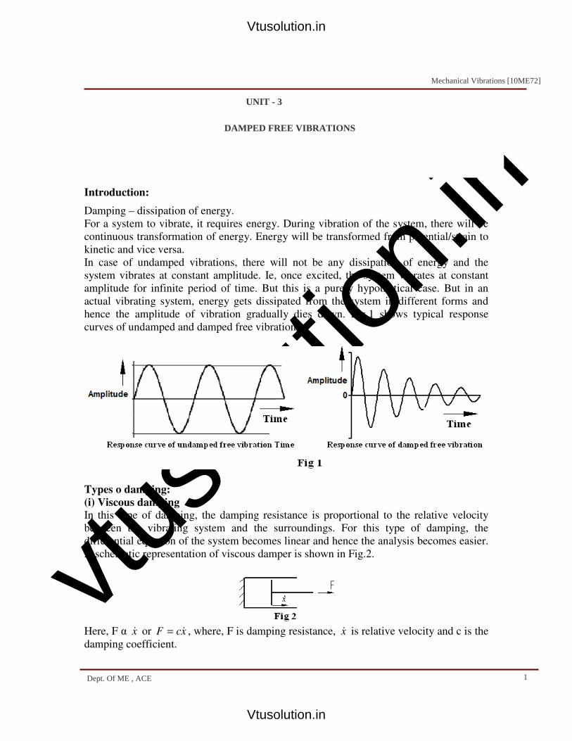
Introduction:
Damping – dissipation of energy.
For a system to vibrate, it requires energy. During vibration of the system, there will be
continuous transformation of energy. Energy will be transformed from potential/strain to
kinetic and vice versa.
In case of undamped vibrations, there will not be any dissipation of energy and the
system vibrates at constant amplitude. Ie, once excited, the system vibrates at constant
amplitude for infinite period of time. But this is a purely hypothetical case. But in an
actual vibrating system, energy gets dissipated from the system in different forms and
hence the amplitude of vibration gradually dies down. Fig.1 shows typical response
curves of undamped and damped free vibrations.
Types o damping:
(i) Viscous damping
In this type of damping, the damping resistance is proportional to the relative velocity
between the vibrating system and the surroundings. For this type of damping, the
differential equation of the system becomes linear and hence the analysis becomes easier.
A schematic representation of viscous damper is shown in Fig.2.
Here, F α x& or xcF &= , where, F is damping resistance, x& is relative velocity and c is the
damping coefficient.
UNIT - 3UNIT - 3
DAMPED FREE VIBRATIONS
Mechanical Vibrations [10ME72]
1Dept. Of ME , ACE
Vtusolution.in
Vtusolution.in

vtuso
lution
.in
2
(ii) Dry friction or Coulomb damping
In this type of damping, the damping resistance is independent of rubbing velocity and is
practically constant.
(iii) Structural damping
This type of damping is due to the internal friction within the structure of the material,
when it is deformed.
Spring-mass-damper system:
Fig.3 shows the schematic of a simple spring-mass-damper system, where, m is the mass
of the system, k is the stiffness of the system and c is the damping coefficient.
If x is the displacement of the system, from Newton’s second law of motion, it can be
written
kxxcxm −−= &&&
Ie 0=++ kxxcxm &&& (1)
This is a linear differential equation of the second order and its solution can be written as st
ex = (2)
Differentiating (2), stsex
dt
dx== &
stesx
dt
xd 2
2
2
== &&
Substituting in (1), 02 =++ stststkecseems
( ) 02 =++ stekcsms
Or 02 =++ kcsms (3)
Equation (3) is called the characteristic equation of the system, which is quadratic in s.
The two values of s are given by
m
k
m
c
m
cs −
±−=
2
2,122
(4)
Mechanical Vibrations [10ME72]
2Dept. Of ME, ACE
Vtusolution.in
Vtusolution.in

vtuso
lution
.in
3
The general solution for (1) may be written as
tstseCeCx 21
21 += (5)
Where, C1 and C2 are arbitrary constants, which can be determined from the initial
conditions.
In equation (4), the values of s1 = s2, when m
k
m
c=
2
2
Or, nm
k
m
cω==
2 (6)
Or nmc ω2= , which is the property of the system and is called critical
damping coefficient and is represented by cc.
Ie, critical damping coefficient = nc mc ω2=
The ratio of actual damping coefficient c and critical damping coefficient cc is called
damping factor or damping ratio and is represented by ζ.
Ie, cc
c=ζ (7)
In equation (4), m
c
2 can be written as n
c
c m
c
c
c
m
cωζ .
22=×=
Therefore, ( ) [ ] nnnns ωζζωωζωζ 1.. 222
2,1 −±−=−±−= (8)
The system can be analyzed for three conditions.
(i) ζ > 1, ie, c > cc, which is called over damped system.
(ii) ζ = 1. ie, c = cc, which is called critically damped system.
(iii) ζ < 1, ie, c < cc, which is called under damped system.
Depending upon the value of ζ, value of s in equation (8), will be real and unequal, real
and equal and complex conjugate respectively.
(i) Analysis of over-damped system (ζ > 1).
In this case, values of s are real and are given by
[ ]ns ωζζ 12
1 −+−= and [ ]ns ωζζ 12
2 −−−=
Then, the solution of the differential equation becomes
tt nn
eCeCxωζζωζζ
−−−
−+−
+=1
2
1
1
22
(9)
This is the final solution for an over damped system and the constants C1 and C2 are
obtained by applying initial conditions. Typical response curve of an over damped system
is shown in fig.4. The amplitude decreases exponentially with time and becomes zero at t
= ∞.
Mechanical Vibrations [10ME72]
3Dept. Of ME, ACE
Vtusolution.in
Vtusolution.in

vtuso
lution
.in
4
(ii) Analysis of critically damped system (ζ = 1).
In this case, based on equation (8), s1 = s2 = -ωn
The solution of the differential equation becomes
tststeCeCx 21
21 +=
Ie, tt nn teCeCx
ωω −−+= 21
Or, ( ) tnetCCxω−
+= 21 (10)
This is the final solution for the critically damped system and the constants C1 and C2 are
obtained by applying initial conditions. Typical response curve of the critically damped
system is shown in fig.5. In this case, the amplitude decreases at much faster rate
compared to over damped system.
Mechanical Vibrations [10ME72]
4Dept. Of ME, ACE
Vtusolution.in
Vtusolution.in

vtuso
lution
.in
5
(iii) Analysis of under damped system (ζ < 1).
In this case, the roots are complex conjugates and are given by
[ ]njs ωζζ 2
1 1−+−=
[ ]njs ωζζ 2
2 1−−−=
The solution of the differential equation becomes
tjtj nn
eCeCxωζζωζζ
−−−
−+−
+=22 1
2
1
1
This equation can be rewritten as
+=
−−
−
−tjtj
t nnn eCeCex
ωζωζζω
22 1
2
1
1 (11)
Using the relationships
θθθ sincos iei +=
θθθ sincos iei −=−
Equation (11) can be written as
{ } { }[ ]tjtCtjtCex nnnn
tn ωζωζωζωζζω 22
2
22
1 1sin1cos1sin1cos −−−+−+−=−
Or ( ){ } ( ){ }[ ]tCCjtCCex nn
tn ωζωζζω 2
21
2
21 1sin1cos −−+−+=−
(12)
In equation (12), constants (C1+C2) and j(C1-C2) are real quantities and hence, the
equation can also be written as
{ } { }[ ]tBtAex nn
tn ωζωζζω 22 1sin1cos −+−=−
Or, ( ){ }[ ]1
2
1 1sin φωζζω+−=
−teAx n
tn (13)
The above equations represent oscillatory motion and the frequency of this motion is
represented by nd ωζω 21−= (14)
Where, ωd is the damped natural frequency of the system. Constants A1 and Φ1 are
determined by applying initial conditions. The typical response curve of an under damped
system is shown in Fig.6.
Mechanical Vibrations [10ME72]
5Dept.Of ME, ACE
Vtusolution.in
Vtusolution.in

vtuso
lution
.in
6
Applying initial conditions,
x = Xo at t = 0; and 0=x& at t = 0, and finding constants A1 and Φ1,
equation (13) becomes
−+−
−= −−
ζ
ζωζ
ζ
ζω2
12
2
1tan1sin
1te
Xx n
to n (15)
The term to ne
X ζω
ζ
−
− 21 represents the amplitude of vibration, which is observed to decay
exponentially with time.
Mechanical Vibrations [10ME72]
6Dept. Of ME, ACE
Vtusolution.in
Vtusolution.in

vtuso
lution
.in
7
LOGARITHMIC DECREMENT
Referring to Fig.7, points A & B represent two successive peak points on the response
curve of an under damped system. XA and XB represent the amplitude corresponding to
points A & B and tA & tB represents the corresponding time.
We know that the natural frequency of damped vibration = nd ωζω 21−= rad/sec.
Therefore, π
ω
2
d
df = cycles/sec
Hence, time period of oscillation =
ndd
ABf
ttωζ
π
ω
π21
221
−===− sec (16)
From equation (15), amplitude of vibration
XA = Anto e
X ζω
ζ
−
− 21
XB = Bnto eX ζω
ζ
−
− 21
Or, ( ) ( )ABnBAn tttt
B
A eeX
X −−−==
ζωζω
Using eqn. (16), 21
2
ζ
πζ
−= e
X
X
B
A
Or, 21
2log
ζ
πζ
−=
B
Ae
X
X
Mechanical Vibrations [10ME72]
7Dept. Of ME, ACE
Vtusolution.in
Vtusolution.in
vtuso
lution
.in
8
This is called logarithmic decrement. It is defined as the logarithmic value of the ratio of
two successive amplitudes of an under damped oscillation. It is normally denoted by δ.
Therefore, δ = 21
2log
ζ
πζ
−=
B
Ae
X
X (17)
This indicates that the ratio of any two successive amplitudes of an under damped system
is constant and is a function of damping ratio of the system.
For small values of ζ, πζδ 2≈
If X0 represents the amplitude at a particular peak and Xn represents the amplitude after
‘n’ cycles, then, logarithmic decrement = δ = =1
0logX
Xe =
2
1logX
Xe ……
n
n
eX
X 1log −=
Adding all the terms, nδ = n
n
eX
X
X
X
X
X 1
2
1
1
0 ......log −×
Or, n
eX
X
n
0log1
=δ (18)
Mechanical Vibrations [10ME72]
8Dept. Of ME, ACE
Vtusolution.in
Vtusolution.in

vtuso
lution
.in
9
Solved problems
1) The mass of a spring-mass-dashpot system is given an initial velocity 5ωn, where
ωn is the undamped natural frequency of the system. Find the equation of motion
for the system, when (i) ζ = 2.0, (ii) ζ = 1.0, (i) ζ = 0.2.
Solution:
Case (i) For ζ = 2.0 – Over damped system
For over damped system, the response equation is given by
tt nn
eCeCxωζζωζζ
−−−
−+−
+=1
2
1
1
22
Substituting ζ = 2.0, [ ] [ ] tt nn eCeCx
ωω 73.3
2
27.0
1
−−+= (a)
Differentiating, t
n
t
nnn eCeCx
ωω ωω 73.3
2
27.0
1 73.327.0−−
−−=& (b)
Substituting the initial conditions
x = 0 at t = 0; and nx ω5=& at t = 0 in (a) & (b),
0 = C1 + C2 (c)
5ωn = -0.27 ωn C1 – 3.73 ωn C2 (d)
Solving (c) & (d), C1 = 1.44 and C2 = -1.44.
Therefore, the response equation becomes
[ ] [ ]( )tt nn eex
ωω 73.327.044.1
−−−= (e)
Case (ii) For ζ = 1.0 – Critically damped system
For critically damped system, the response equation is given by
( ) tnetCCxω−
+= 21 (f)
Differentiating, ( ) tt
nnn eCetCCx
ωωω −−++−= 221
& (g)
Substituting the initial conditions
x = 0 at t = 0; and nx ω5=& at t = 0 in (f) & (g),
C1 = 0 and C2 = 5ωn
Substituting in (f), the response equation becomes
( ) t
nnetx
ωω −= 5 (h)
Case (iii) For ζ = 0.2 – under damped system
For under damped system, the response equation is given by
{ }[ ]1
2
1 1sin φωζζω+−=
−teAx n
tn
Substituting ζ = 0.2, ( ){ }[ ]1
2.0
1 98.0sin φωω+=
−teAx n
tn (p)
Mechanical Vibrations [10ME72]
9Dept. Of ME, ACE
Vtusolution.in
Vtusolution.in

vtuso
lution
.in
10
Differentiating,
( ){ }[ ] ( )1
2.0
11
2.0
1 98.0cos98.098.0sin2.0 φωωφωω ωω+++−=
−−teAteAx n
t
nn
t
nnn& (q)
Substituting the initial conditions
x = 0 at t = 0; and nx ω5=& at t = 0 in (p) & (q),
A1sinΦ1 = 0 and A1 cosΦ1 = 5.1
Solving, A1 = 5.1 and Φ1 = 0
Substituting in (p), the response equation becomes
( ){ }[ ]tex n
tn ωω98.0sin1.5
2.0−= (r)
2) A mass of 20kg is supported on two isolators as shown in fig.Q.2. Determine the
undamped and damped natural frequencies of the system, neglecting the mass of the
isolators.
Solution:
Equivalent stiffness and equivalent damping coefficient are calculated as
30000
13
3000
1
10000
1111
21
=+=+=kkkeq
300
4
100
1
300
1111
21
=+=+=CCCeq
Undamped natural frequency = sec/74.1020
1330000
radm
keq
n ===ω
cpsf n 71.12
74.10==
π
Damped natural frequency = nd ωζω 21−=
1745.0
2013
300002
4300
2=
××
==mk
C
eq
eqζ
Mechanical Vibrations [10ME72]
10Dept. Of ME, ACE
Vtusolution.in
Vtusolution.in

vtuso
lution
.in
11
sec/57.1074.101745.01 2radd =×−=∴ω
Or, cpsf d 68.12
57.10=
×=
π
3) A gun barrel of mass 500kg has a recoil spring of stiffness 3,00,000 N/m. If the
barrel recoils 1.2 meters on firing, determine,
(a) initial velocity of the barrel
(b) critical damping coefficient of the dashpot which is engaged at the end of the
recoil stroke
(c) time required for the barrel to return to a position 50mm from the initial
position.
Solution:
(a) Strain energy stored in the spring at the end of recoil:
mNkxP −=××== 2160002.13000002
1
2
1 22
Kinetic energy lost by the gun barrel:
222 2505002
1
2
1vvmvT =××== , where v = initial velocity of the barrel
Equating kinetic energy lost to strain energy gained, ie T = P,
216000250 2 =v
v = 29.39m/s
(b) Critical damping coefficient = mNkmCc sec/2449550030000022 −=×==
(c) Time for recoiling of the gun (undamped motion):
Undamped natural frequency = srm
kn /49.24
500
300000===ω
Time period = sec259.029.24
22===
π
ω
πτ
n
Time of recoil = sec065.04
259.0
4==
τ
Time taken during return stroke:
Response equation for critically damped system = ( ) tnetCCxω−
+= 21
Differentiating, ( ) t
n
t nn etCCeCxωω ω −−
+−= 212&
Applying initial conditions, x = 1.2, at t = 0 and 0=x& at t = 0,
C1 = 1.2, & C2 = 29.39
Therefore, the response equation = ( ) tetx 49.2439.292.1 −+=
When x = 0.05m, by trial and error, t = 0.20 sec
Therefore, total time taken = time for recoil + time for return = 0.065 + 0.20 = 0.265 sec
The displacement – time plot is shown in the following figure.
Mechanical Vibrations [10ME72]
11Dept. Of ME, ACE
Vtusolution.in
Vtusolution.in

vtuso
lution
.in
12
4) A 25 kg mass is resting on a spring of 4900 N/m and dashpot of 147 N-se/m in
parallel. If a velocity of 0.10 m/sec is applied to the mass at the rest position, what
will be its displacement from the equilibrium position at the end of first second?
Solution:
The above figure shows the arrangement of the system.
Critical damping coefficient = nc mc ω2=
Where srm
kn /14
25
4900===ω
Therefore, mNcc sec/70014252 −=××=
Since C< Cc, the system is under damped and 21.0700
147===
cc
cζ
Mechanical Vibrations [10ME72]
12Dept. Of ME, ACE
Vtusolution.in
Vtusolution.in

vtuso
lution
.in
13
Hence, the response equation is ( ){ }[ ]1
2
1 1sin φωζζω+−=
−teAx n
tn
Substituting ζ and ωn, ( ){ }[ ]1
21421.0
1 1421.01sin φ+−= ×− teAx t
( ){ }[ ]1
94.2
1 7.13sin φ+= − teAx t
Differentiating, ( ){ }[ ] ( )1
94.2
11
94.2
1 7.13cos7.137.13sin94.2 φφ +++−= −− teAteAx tt&
Applying the initial conditions, x = 0, at t = 0 and smx /10.0=& at t = 0
Φ1 = 0
( ){ }[ ] ( )1111 cos7.13sin94.210.0 φφ AA +−=
Since, Φ1 = 0, 0.10 = 13.7 A1; A1 = 0.0073
Displacement at the end of 1 second = ( ){ }[ ] mex 494.2 105.37.13sin0073.0 −− ×==
5) A rail road bumper is designed as a spring in parallel with a viscous damper.
What is the bumper’s damping coefficient such that the system has a damping ratio
of 1.25, when the bumper is engaged by a rail car of 20000 kg mass. The stiffness of
the spring is 2E5 N/m. If the rail car engages the bumper, while traveling at a speed
of 20m/s, what is the maximum deflection of the bumper?
m
k
c
Solution: Data = m = 20000 kg; k = 200000 N/m; 25.1=ζ
Critical damping coefficient =
mNkmcc sec/1024.12000002000022 5 −×=××=××=
Damping coefficient mNCC C sec/1058.11024.125.1 55 −×=××=×= ζ
Undamped natural frequency = srm
kn /16.3
20000
200000===ω
Since 25.1=ζ , the system is over damped.
For over damped system, the response equation is given by
tt nn
eCeCxωζζωζζ
−−−
−+−
+=1
2
1
1
22
Substituting ζ = 1.25, [ ] [ ] tt nn eCeCx
ωω 0.2
2
5.0
1
−−+= (a)
Mechanical Vibrations [10ME72]
13Dept. Of ME, ACE
Vtusolution.in
Vtusolution.in

vtuso
lution
.in
14
Differentiating, t
n
t
nnn eCeCx
ωω ωω 0.2
2
5.0
1 0.25.0−−
−−=& (b)
Substituting the initial conditions
x = 0 at t = 0; and smx /20=& at t = 0 in (a) & (b),
0 = C1 + C2 (c)
20 = -0.5 ωn C1 – 2.0 ωn C2 (d)
Solving (c) & (d), C1 = 4.21and C2 = -4.21
Therefore, the response equation becomes
[ ] [ ]( )meex tt ×−×− −= 32.658.121.4 (e)
The time at which, maximum deflection occurs is obtained by equating velocity equation
to zero.
Ie, 00.25.00.2
2
5.0
1 =−−=−− t
n
t
nnn eCeCx
ωω ωω&
Ie, 061.2665.6 32.658.1 =+− −− ttee
Solving the above equation, t = 0.292 secs.
Therefore, maximum deflection at t = 0.292secs,
Substituting in (e), [ ] [ ]( )meex 292.032.6292.058.121.4 ×−×− −= , = 1.99m.
6) A disc of a torsional pendulum has a moment of inertia of 6E-2 kg-m2 and is
immersed in a viscous fluid. The shaft attached to it is 0.4m long and 0.1m in
diameter. When the pendulum is oscillating, the observed amplitudes on the same
side of the mean position for successive cycles are 90, 6
0 and 4
0. Determine (i)
logarithmic decrement (ii) damping torque per unit velocity and (iii) the periodic
time of vibration. Assume G = 4.4E10 N/m2, for the shaft material.
Shaft dia. = d = 0.1m
Shaft length = l = 0.4m
Moment of inertia of disc = J = 0.06 kg-m2.
Modulus of rigidity = G = 4.4E10 N/m2
Solution: The above figure shows the arrangement of the system.
(i) Logarithmic decrement = 405.04
6log
6
9log === eeδ
(ii) The damping torque per unit velocity = damping coefficient of the system ‘C’.
Mechanical Vibrations [10ME72]
14Dept. Of ME, ACE
Mechanical Vibrations [10ME72]Mechanical Vibrations [10ME72]
Vtusolution.in
Vtusolution.in

vtuso
lution
.in
15
We know that logarithmic decrement = 21
2
ζ
πζδ
−= , rearranging which, we get
Damping factor 0645.0405.04
405.0
4 2222=
+=
+=
πδπ
δζ
Also, CC
C=ζ , where, critical damping coefficient = JkC tC 2=
Torsional stiffness = radmNd
l
G
l
GIk
p
t /1008.132
1.0
4.0
104.4
32
64104
−×=×
××
=×==ππ
Critical damping coefficient = radmNJkC tC /50906.01008.122 6 −=××==
Damping coefficient of the system = radmNCC C /8.320645.0509 −=×=×= ζ
(iii) Periodic time of vibration = 21
221
ζω
π
ω
πτ
−===
nddf
Where, undamped natural frequency = sec/6.424206.0
1008.1 6
radJ
kt
n =×
==ω
Therefore, sec00148.00645.016.4242
2
2=
−×=
πτ
7) A mass of 1 kg is to be supported on a spring having a stiffness of 9800 N/m. The
damping coefficient is 5.9 N-sec/m. Determine the natural frequency of the system.
Find also the logarithmic decrement and the amplitude after three cycles if the
initial displacement is 0.003m.
Solution:
Undamped natural frequency = srm
kn /99
1
9800===ω
Damped natural frequency = nd ωζω 21−=
Critical damping coefficient = mNmc nc sec/19899122 −=××=××= ω
Damping factor = 03.0198
9.5===
cc
cζ
Hence damped natural frequency = sec/99.9899013.011 22radnd =×−=−= ωζω
Mechanical Vibrations [10ME72]
15Dept. Of ME, ACE
Vtusolution.in
Vtusolution.in

vtuso
lution
.in
16
Logarithmic decrement = 188.003.01
03.02
1
2
22=
−
××=
−=
π
ζ
πζδ
Also, n
eX
X
n
0log1
=δ ; if x0 = 0.003,
then, after 3 cycles, 3
0 003.0log
3
1188.0,log
1
Xie
X
X
ne
n
e ×==δ
ie, me
X3
188.033 1071.1003.0 −
××==
8) The damped vibration record of a spring-mass-dashpot system shows the
following data.
Amplitude on second cycle = 0.012m; Amplitude on third cycle = 0.0105m;
Spring constant k = 7840 N/m; Mass m = 2kg. Determine the damping constant,
assuming it to be viscous.
Solution:
Here, 133.00105.0
012.0loglog
3
2 === eeX
Xδ
Also, 21
2
ζ
πζδ
−= , rearranging, 021.0
133.04
133.0
4 2222=
+=
+=
πδπ
δζ
Critical damping coefficient = mNkmcc sec/4.2507840222 −=××=××=
Damping coefficient mNCC C sec/26.54.250021.0 −=×=×= ζ
9) A mass of 2kg is supported on an isolator having a spring scale of 2940 N/m and
viscous damping. If the amplitude of free vibration of the mass falls to one half its
original value in 1.5 seconds, determine the damping coefficient of the isolator.
Solution:
Undamped natural frequency = srm
kn /34.38
2
2940===ω
Mechanical Vibrations [10ME72]Mechanical Vibrations[10ME72]
16Dept.Of ME, ACE
Vtusolution.in
Vtusolution.in

vtuso
lution
.in
17
Critical damping coefficient = mNmc nc sec/4.15334.38222 −=××=××= ω
Response equation of under damped system = ( ){ }[ ]1
2
1 1sin φωζζω+−=
−teAx n
tn
Here, amplitude of vibration =tneA
ζω−
1
If amplitude = X0 at t = 0, then, at t = 1.5 sec, amplitude = 2
0X
Ie, 0
0
1 XeA n =×−ζω
or 01 XA =
Also, 2
05.1
1
XeA n =
×−ζω or
2
05.134.38
0
XeX =× ××−ζ or
2
15.134.38 =××−ζe
Ie, 25.134.38 =××ζe , taking log, 012.069.05.134.38 =∴=×× ζζ
Damping coefficient mNCC C sec/84.14.153012.0 −=×=×= ζ
Mechanical Vibrations [10ME72]
17Dept. Of ME, ACE
Vtusolution.in
Vtusolution.in

vtuso
lution
.in
Forced Vibrations Dr. M.A.Kamoji
KLE CET Belgaum
Introduction: In free un-damped vibrations a system once disturbed from its initial
position executes vibrations because of its elastic properties. There is no
damping in these systems and hence no dissipation of energy and hence it
executes vibrations which do not die down. These systems give natural
frequency of the system.
In free damped vibrations a system once disturbed from its position will
execute vibrations which will ultimately die down due to presence of
damping. That is there is dissipation of energy through damping. Here one
can find the damped natural frequency of the system.
In forced vibration there is an external force acts on the system. This
external force which acts on the system executes the vibration of the system.
The external force may be harmonic and periodic, non-harmonic and
periodic or non periodic. In this chapter only external harmonic forces acting
on the system are considered. Analysis of non harmonic forcing functions is
just an extension of harmonic forcing functions.
Examples of forced vibrations are air compressors, I.C. engines, turbines,
machine tools etc,.
Analysis of forced vibrations can be divided into following categories as per
the syllabus.
1. Forced vibration with constant harmonic excitation
2. Forced vibration with rotating and reciprocating unbalance
3. Forced vibration due to excitation of the support
A: Absolute amplitude
UNIT - 4
FORCESUNIT - 4
FORCED VIBRATIONS
Mechanical Vibrations [10ME72]
1Dept. Of ME, ACE
Vtusolution.in
Vtusolution.in

vtuso
lution
.in
B: Relative amplitude
4. Force and motion transmissibility
For the above first a differential equation of motion is written. Assume a
suitable solution to the differential equation. On obtaining the suitable
response to the differential equation the next step is to non-dimensional the
response. Then the frequency response and phase angle plots are drawn.
1. Forced vibration with constant harmonic excitation
From the figure it is evident that spring force and damping force oppose the
motion of the mass. An external excitation force of constant magnitude acts
on the mass with a frequency ω. Using Newton’s second law of motion an
equation can be written in the following manner.
Equation 1 is a linear non homogeneous second order differential equation.
The solution to eq. 1 consists of complimentary function part and particular
1tSinωFkxxcxm o −−−−−−=++ &&&
Mechanical Vibrations [10ME72]
2Dept. Of ME, ACE
Vtusolution.in
Vtusolution.in

vtuso
lution
.in
integral. The complimentary function part of eq, 1 is obtained by setting the
equation to zero. This derivation for complementary function part was done
in damped free vibration chapter.
The complementary function solution is given by the following equation.
Equation 3 has two constants which will have to be determined from the
initial conditions. But initial conditions cannot be applied to part of the
solution of eq. 1 as given by eq. 3. The complete response must be
determined before applying the initial conditions. For complete response the
particular integral of eq. 1 must be determined. This particular solution will
be determined by vector method as this will give more insight into the
analysis.
Assume the particular solution to be
Differentiating the above assumed solution and substituting it in eq. 1
[ ] 3φtωξ1SineAx 2n2tζω
2cn −−−+−=
−
2xxx pc −−−−−+=
( ) 4φωtXSinxp −−−−−=
( )πφωtXSinωx
2
πφωtωXSinx
2
p
p
+−=
+−=
&&
&
( )
( ) 50πφωtXSinmω
2
πφωtxcωφωtkXSintSinωF
2
o
−−−−−=+−−
+−−−−
Mechanical Vibrations [10ME72]
3Dept. Of ME, ACE
Vtusolution.in
Vtusolution.in

vtuso
lution
.in
Fig. Vector representation of forces on system subjected to forced vibration
Following points are observed from the vector diagram
1. The displacement lags behind the impressed force by an angle Φ.
2. Spring force is always opposite in direction to displacement.
3. The damping force always lags the displacement by 90°. Damping
force is always opposite in direction to velocity.
4. Inertia force is in phase with the displacement.
The relative positions of vectors and heir magnitudes do not change with
time.
From the vector diagram one can obtain the steady state amplitude and
phase angle as follows
Mechanical Vibrations [10ME72]
4Dept. Of ME, ACE
Vtusolution.in
Vtusolution.in

vtuso
lution
.in
The above equations are made non-dimensional by dividing the numerator
and denominator by K.
where, is zero frequency deflection
Therefore the complete solution is given by
( ) ( )[ ] 6cωmωkFX222
0 −−−+−=
( )[ ] 7mωkcωtanφ 2-1 −−−−=
( )[ ] ( )[ ]
( )( )
92
nωω1
nωω2ξ
tan 1-φ
8
ωω2ξωω1
XX
2
n
22
n
st
−−−−
=
−−−
+−
=
kFX ost =
pc xxx +=
[ ]( )
( )[ ] ( )[ ]10
ωω2ξωω1
φωtSinX
φtωξ1SineAx
2
n
22
n
st
2n
2tζω
2n
−−−
+−
−+
+−= −
Mechanical Vibrations [10ME72]
5Dept. Of ME, ACE
Vtusolution.in
Vtusolution.in

vtuso
lution
.in
The two constants A2 and φ2 have to be determined from the initial
conditions.
The first part of the complete solution that is the complementary function
decays with time and vanishes completely. This part is called transient
vibrations. The second part of the complete solution that is the particular
integral is seen to be sinusoidal vibration with constant amplitude and is
called as steady state vibrations. Transient vibrations take place at damped
natural frequency of the system, where as the steady state vibrations take
place at frequency of excitation. After transients die out the complete
solution consists of only steady state vibrations.
In case of forced vibrations without damping equation 10 changes to
Φ2 is either 0° or 180° depending on whether ω<ωn or ω>ωn
Steady state Vibrations: The transients die out within a short period of
time leaving only the steady state vibrations. Thus it is important to know
the steady state behavior of the system,
Thus Magnification Factor (M.F.) is defined as the ratio of steady state
amplitude to the zero frequency deflection.
[ ]( )
( )11
ωω1
ωtSinXφtωSinAx
2
n
st2n2 −−−
−++=
( )[ ] ( )[ ]12
ωω2ξωω1
1
X
XM.F.
2
n
22
nst
−−−
+−
==
( )( )
132
nωω1
nωω2ξ
tan 1-φ −−−−
=
Mechanical Vibrations [10ME72]
6Dept. Of ME, ACE
Vtusolution.in
Vtusolution.in

vtuso
lution
.in
Equations 12 and 13 give the magnification factor and phase angle. The
steady state amplitude always lags behind the impressed force by an angle
Φ. The above equations are used to draw frequency response and phase
angle plots.
Fig. Frequency response and phase angle plots for system subjected forced
vibrations.
Frequency response plot: The curves start from unity at frequency ratio of
zero and tend to zero as frequency ratio tends to infinity. The magnification
factor increases with the increase in frequency ratio up to 1 and then
decreases as frequency ratio is further increased. Near resonance the
amplitudes are very high and decrease with the increase in the damping
ratio. The peak of magnification factor lies slightly to the left of the
resonance line. This tilt to the left increases with the increase in the damping
ratio. Also the sharpness of the peak of the curve decreases with the increase
in the damping.
Mechanical Vibrations [10ME72]
7Dept. OF ME, ACE
Vtusolution.in
Vtusolution.in

vtuso
lution
.in
Phase angle plot: At very low frequency the phase angle is zero. At
resonance the phase angle is 90°. At very high frequencies the phase angle
tends to 180°. For low values of damping there is a steep change in the phase
angle near resonance. This decreases with the increase in the damping. The
sharper the change in the phase angle the sharper is the peak in the
frequency response plot.
The amplitude at resonance is given by equation 14
The frequency at which maximum amplitude occurs is obtained by
differentiating the magnification factor equation with respect to frequency
ratio and equating it to zero.
Also no maxima will occur for or
2. Rotating and Reciprocating Unbalance
Machines like electric motors, pumps, fans, clothes dryers, compressors
have rotating elements with unbalanced mass. This generates centrifugal
type harmonic excitation on the machine.
The final unbalance is measured in terms of an equivalent mass mo rotating
with its c.g. at a distance e from the axis of rotation. The centrifugal force is
proportional to the square of frequency of rotation. It varies with the speed
142ξXX
FX cω
str
or
−−−=
=
152ξ1ω
ω2
n
p−−−−=
⟩
2
1ξ 707.0⟩ξ
Mechanical Vibrations [10ME72]
Dept. Of ME, ACE 8
Vtusolution.in
Vtusolution.in
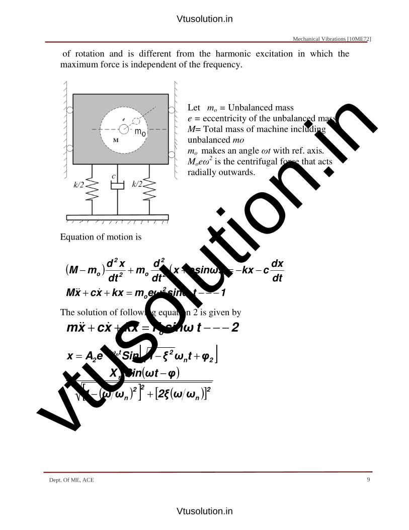
vtuso
lution
.in
of rotation and is different from the harmonic excitation in which the
maximum force is independent of the frequency.
Let mo = Unbalanced mass
e = eccentricity of the unbalanced mass
M= Total mass of machine including
unbalanced mo
mo makes an angle ωt with ref. axis.
Moeω2 is the centrifugal force that acts
radially outwards.
Equation of motion is
The solution of following equation 2 is given by
( ) ( )
1t sinωeωmkxxcxM
dt
dxckxesinωsx
dt
dm
dt
xdmM
2o
2
2
o2
2
o
−−−=++
−−=++−
&&&
2t sinωFkxxcxm o −−−=++ &&&
[ ]( )
( )[ ] ( )[ ]2n
22
n
st
2n
2tζω
2
ωω2ξωω1
φωtSinX
φtωξ1SineAx n
+−
−+
+−= −
Mechanical Vibrations [10ME72]
9Dept. Of ME, ACE
Vtusolution.in
Vtusolution.in

vtuso
lution
.in
Compare eq. 1 with eq.2 the only change is Fo is replaced by mo eω2
The transient part of the solution remains the same. The only change is in the
steady state part of the solution.
Therefore the steady state solution of eq.1 can be written as
The above equation reduces to dimensionless form as
The phase angle equation and its plot remains the same as shown below
( )
222
2o
k
cω
k
Mω1
keωmwhere...X
φωtXsinx
+
−
=
−=
2
n
22
n
2
n
2o
ω
ω2ξ
ω
ω1
ω
ω
M
eωm
X
+
−
=
−
= −
2
n
n1
ω
ω1
ω
ω2ξ
tanφ
Mechanical Vibrations[10ME72]
10Dept. Of ME, ACE
Vtusolution.in
Vtusolution.in

vtuso
lution
.in
Frequency response and phase angle plots (Unbalance)
At low speeds is small, hence all response curves start
from zero.
At resonance ω / ωn = 1, therefore
And amplitude is limited due to damping present in the system. Under these
conditions the motion of main mass (M-mo) lags that of the mass mo by 90°.
When ω / ωn is very large the ratio X/(moe/M) tends to unity and the main
mass (M-mo) has an amplitude of X= moe/M . This motion is 180° out of
phase with the exciting force. That is when unbalanced mass moves up, the
main mass moves down and vice versa.
Problem 1
A counter rotating eccentric weight exciter is used to produce the forced
oscillation of a spring-supported mass as shown in Fig. By varying the speed
2222ξξξξ1111
MMMMeeeemmmm
XXXXoooo =
Mechanical Vibrations [10ME72]
11Dept. Of ME, ACE
Vtusolution.in
Vtusolution.in

vtuso
lution
.in
of rotation, a resonant amplitude of 0.60 cm was recorded. When the speed
of rotation was increase considerably beyond the resonant frequency, the
amplitude appeared to approach a fixed value of 0.08 cm. Determine the
damping factor of the system.
Dividing one by the other
(Answer)
Problem 2
A system of beam supports a mass of 1200 kg. The motor has an unbalanced
mass of 1 kg located at 6 cm radius. It is known that the resonance occurs at
2210 rpm. What amplitude of vibration can be expected at the motors
operating speed of 1440 rpm if the damping factor is assumed to be less than
0.1
Solution:
Given: M = 1200 kg, mo= 1 kg, eccentricity = e = 0.06m, Resonance at 2210
rpm, Operating speed = 1440 rpm, ξ = 0.1, X = ?.
0.6cm0.6cm0.6cm0.6cm2222ξξξξMMMMeeeemmmm
XXXXoooo
==
0.08cm0.08cm0.08cm0.08cmMMMMeeeemmmmXXXX oooo ==
0.06670.06670.06670.0667ξξξξ =
ssss / / / /radradradrad 231.43231.43231.43231.4360606060
NNNN 2222ππππωωωωnnnn == s150.79rad/60
N 2πω
op==
0.652rω
ω
n
==
2222nnnn22222222nnnn nnnn2222ooooωωωωωωωω2222ξξξξωωωω
ωωωω1111
ωωωωωωωω
MMMMeeeeωωωωmmmmXXXX
+
−
=
2
Mechanical Vibrations[10ME72]
12Dept. Of ME, ACE
Vtusolution.in
Vtusolution.in

vtuso
lution
.in
Substituting the appropriate values in the above eq.
X = 0.036 mm (Answer)
However, if ξ is made zero, the amplitude X = 0.037 mm (Answer)
This means if the damping is less than 0.1, the amplitude of vibration will be
between 0.036 mm and 0.037 mm. (Answer)
Problem 3
An eccentric mass exciter is used to determine the vibratory characteristics
of a structure of mass 200 kg. At a speed of 1000 rpm a stroboscope showed
the eccentric mass to be at the bottom position at the instant the structure
was moving downward through its static equilibrium position and the
corresponding amplitude was 20 mm. If the unbalance of the eccentric is
0.05 kg-m, determine, (a) un damped natural frequency of the system (b) the
damping factor of the structure (c) the angular position of the eccentric at
1300 rpm at the instant when the structure is moving downward through its
equilibrium position.
Solution:
Given: M = 200 kg, Amplitude at 1000 rpm = 20 mm, moe = 0.05 kg-m
At 1000 rpm the eccentric mass is at the bottom when the structure was
moving downward – This means a there is phase lag of 90° (i.e., at
resonance). At resonance ω = ωn.
(Answer) (Answer)
0.00625ξ
2ξ
1
M
em
X
s104.72rad/60
N 2πωω
o
n
=
=
===
oooo 2222nnnnnnnn1111176.89176.89176.89176.89φφφφ
ωωωωωωωω1111ωωωωωωωω2222ξξξξ
tantantantan
=
−
= −φφφφ
Mechanical Vibrations [10ME72]
13Dept. Of ME, ACE
Vtusolution.in
Vtusolution.in

vtuso
lution
.in
Problem 4
A 40 kg machine is supported by four springs each of stiffness 250 N/m.
The rotor is unbalanced such that the unbalance effect is equivalent to a
mass of 5 kg located at 50mm from the axis of rotation. Find the amplitude
of vibration when the rotor rotates at 1000 rpm and 60 rpm. Assume
damping coefficient to be 0.15
Solution:
Given: M = 40 kg, mo= 5 kg, e = .05 m, ξ = 0.15, N = 1000 rpm and 60 rpm.
When N = 1000 rpm
X at 1000 rpm = 6.26 mm (Solution)
When N = 60 rpm
Using the same eq. X at 60 rpm = 14.29 mm (Solution)
Problem 5
A vertical single stage air compressor having a mass of 500 kg is mounted
on springs having a stiffness of 1.96×10⁵ N/m and a damping coefficient of
0.2. The rotating parts are completely balanced and the equivalent
reciprocating parts have a mass of 20 kg. The stroke is 0.2 m. Determine the
5rad/sM
kω
s104.67rad/60
N 2πω
n ==
==
20.934ω
ω
n
=
2222nnnn22222222nnnn nnnn2222ooooωωωωωωωω2222ξξξξωωωω
ωωωω1111
ωωωωωωωω
MMMMeeeeωωωωmmmmXXXX
+
−
=
2
1.256ω
ω
6.28rad/s60
N 2πω
n
=
==
Mechanical Vibrations [10Me72]
14Dept. Of ME, ACE
Vtusolution.in
Vtusolution.in

vtuso
lution
.in
dynamic amplitude of vertical motion and the phase difference between the
motion and excitation force if the compressor is operated at 200 rpm.
Solution
Given: M = 500 kg, k = 1.96×10⁵ N/m, ξ = 0.2, mo = 20 kg, stroke = 0.2 m, N
= 200 rpm, X = ?.
Stroke = 0.2 m, i.e. eccentricity e = stroke/2 = 0.1 m
Using the equations X = 10.2 mm and φ = 105.9° (Solution)
(a)
(Solution)
(b)
X = 0.15 cm and φ = 169° (Solution)
(c)
(d)
0.175715.5
125
c
cξ
s/m715.54N2064002kM2c
s/m125N4500c
c
c
===
−=×==
−==
2222nnnn22222222nnnn nnnn2222ooooωωωωωωωω2222ξξξξωωωω
ωωωω1111
ωωωωωωωω
MMMMeeeeωωωωmmmmXXXX
+
−
=
2
−
= − 2222nnnnnnnn1111ωωωωωωωω1111ωωωωωωωω2222ξξξξ
tantantantanφφφφ
0.357cmM 2ξ
emX
170.74rpmπ2
ω60N
17.88rad/s20
6400
M
kω
or
nr
n
==
=×
×=
===
( ) ( ) 12.4NkXX cωF
9.6N100.156400kX
7.85N100.1560
400π2125X cω
22
2
2
=+=
=××=
=××××
×=
−
−
Mechanical Vibrations [10ME72]
15Dept.Of ME, ACE
Vtusolution.in
Vtusolution.in
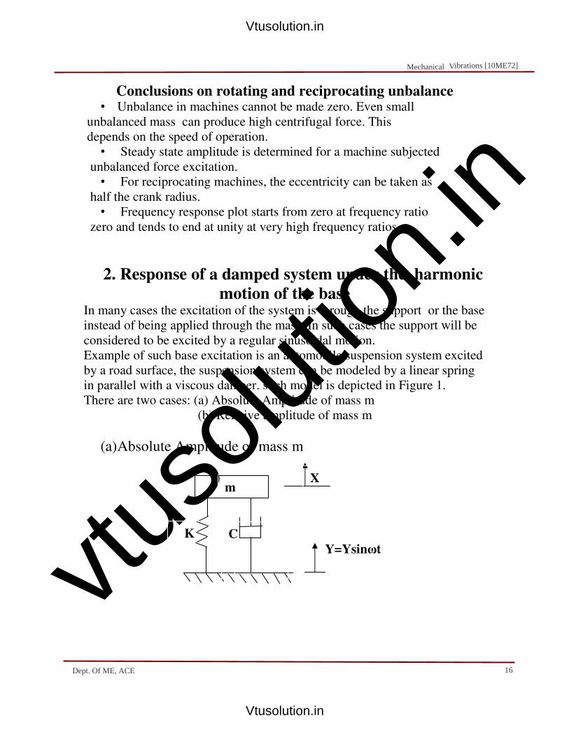
vtuso
lution
.in
Conclusions on rotating and reciprocating unbalance • Unbalance in machines cannot be made zero. Even small
unbalanced mass can produce high centrifugal force. This
depends on the speed of operation.
• Steady state amplitude is determined for a machine subjected
unbalanced force excitation.
• For reciprocating machines, the eccentricity can be taken as
half the crank radius.
• Frequency response plot starts from zero at frequency ratio
zero and tends to end at unity at very high frequency ratios.
2. Response of a damped system under the harmonic
motion of the base In many cases the excitation of the system is through the support or the base
instead of being applied through the mass. In such cases the support will be
considered to be excited by a regular sinusoidal motion.
Example of such base excitation is an automobile suspension system excited
by a road surface, the suspension system can be modeled by a linear spring
in parallel with a viscous damper. such model is depicted in Figure 1.
There are two cases: (a) Absolute Amplitude of mass m
(b) Relative amplitude of mass m
(a) Absolute Amplitude of mass m
m
Y=Ysinωt
K C
X
Mechanical Vibrations [10ME72]
16Dept. Of ME, ACE
Vtusolution.in
Vtusolution.in

vtuso
lution
.in
It is assumed that the base moves harmonically, that is
where Y denotes the amplitude of the base motion and ω represents the
frequency of the base excitation
Substituting Eq.2 in Eq. 1
The above equation can be expressed as
where Y[k2 + (c ω )
2]
1/2 is the amplitude of excitation force.
Examination of equation 3 reveals that it is identical to an Equation
developed during derivation for M.F. The solution is:
( )φφφφωtωtωtωtXsinXsinXsinXsinxxxx −=
=++ tFkxxcxm o ωsin&&&
Mechanical Vibrations [10ME72]
17Dept. Of ME, ACE
Vtusolution.in
Vtusolution.in

vtuso
lution
.in
Therefore the steady state amplitude and phase angle to eq. 3 is
The above equations can be written in dimensionless form
as follows
( )[ ] ( )[ ]2222nnnn22222222nnnn ooooωωωωωωωω2222ξξξξωωωωωωωω1111
kkkkFFFFXXXX+−
=
( )φφφφ----ααααωtωtωtωtXsinXsinXsinXsinxxxx +=
2222nnnn22222222nnnn2222nnnnωωωωωωωω2222ξξξξωωωω
ωωωω1111
ωωωωωωωω2222ξξξξ1111
YYYYXXXX
+
−
+
=
−
= − 2222nnnnnnnn1111ωωωωωωωω1111ωωωωωωωω2222ξξξξ
tantantantanφφφφ
Mechanical Vibrations [10ME72]
18Dept. Of ME, ACE
Vtusolution.in
Vtusolution.in
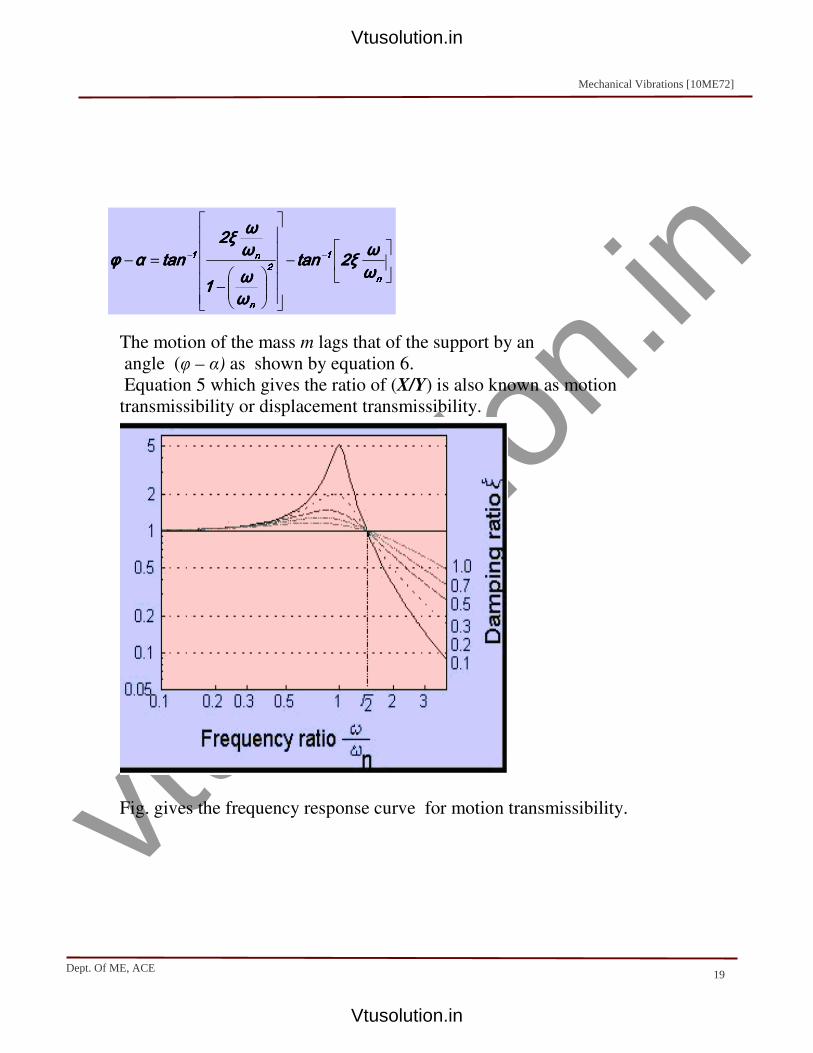
vtuso
lution
.in
The motion of the mass m lags that of the support by an
angle (φ – α) as shown by equation 6.
Equation 5 which gives the ratio of (X/Y) is also known as motion
transmissibility or displacement transmissibility.
Fig. gives the frequency response curve for motion transmissibility.
−
−
=− −− nnnn11112222nnnnnnnn1111ωωωωωωωω2222ξξξξtantantantan
ωωωωωωωω1111ωωωωωωωω2222ξξξξ
tantantantanααααφφφφ
Mechanical Vibrations [10ME72]
19Dept. Of ME, ACE
Vtusolution.in
Vtusolution.in

vtuso
lution
.in
1. For low frequency ratios the system moves as a rigid body and X/Y
�1.
2. At resonance the amplitudes are large
3. For very high frequency ratios the body is almost stationary (X/Y � 0)
It will seen later that the same response curve is also used for Force
Transmissibility.
(b) Relative Amplitude of mass m
Here amplitude of mass m relative to the base motion is considered. The
equations are basically made use in the
Seismic instruments. If z represents the relative motion of the mass w.r.t.
support,
Substituting the value of x in eq.
The above equation is similar to the equation developed for rotating and
reciprocating unbalances. Thus the relative steady state amplitude can
written as
zyx
yxz
+=
−=
tY ωsin2mωkzzczm =++ &&&
2222nnnn22222222nnnn nnnnωωωωωωωω2222ξξξξωωωω
ωωωω1111
ωωωωωωωω
YYYYZZZZ
+
−
=
2 ( )( )
=
− 21
2
n
n
ωω
ωωξφ 1-tan
Mechanical Vibrations [10ME72]
20Dept. OF ME, ACE
Vtusolution.in
Vtusolution.in

vtuso
lution
.in
Thus eq. 7 and eq.8 are similar to the one developed during the study
of rotating an reciprocating unbalances. Frequency and phase response plots
will also remain same.
Problem 1
The support of a spring mass system is vibrating with an amplitude of 5 mm
and a frequency of 1150 cpm. If the mass is 0.9 kg and the stiffness of
springs is 1960 N/m, Determine the amplitude of vibration of mass. What
amplitude will result if a damping factor of 0.2 is included in the system.
Solution:
Given: Y = 5 mm, f = 1150cpm, m =0.9 kg, k = 1960 N/m, X = ?
ξ = 0.2, then X = ?
When ξ = 0, X = 0.886 mm (Solution)
When ξ = 0.2, X = 1.25 mm (Solution)
46.67rad/s0.9
1960
m
kωn ===
s120.43rad/1150/60π2fπ2ω =××=××=
2.58rω
ω
n
==
2222nnnn22222222nnnn2222nnnnωωωωωωωω2222ξξξξωωωω
ωωωω1111
ωωωωωωωω2222ξξξξ1111
YYYYXXXX
+
−
+
=
Mechanical Vibrations [10ME72]
21Dept.Of ME, ACE
Vtusolution.in
Vtusolution.in

vtuso
lution
.in
Observe even when damping has increased the amplitude has not decreased
but it has increased.
Problem 2
The springs of an automobile trailer are compressed 0.1 m under its own
weight. Find the critical speed when the trailer is travelling over a road with
a profile approximated by a sine wave of amplitude 0.08 m and a
wavelength of 14 m. What will be the amplitude of vibration at 60 km/hr.
Solution:
Given: Static deflection = dst = 0.1 m, Y = 0.08 m, γ = 14 m, Critical Speed
= ?, X60 = ?.
Critical speed can be found by finding natural frequency.
Corresponding V = 22.06 m/s = 79.4 km/hr
Amplitude X at 60 km/hr
V60 = 16.67 m/s
When damping is zero X at 60km/hr = 0.186 m (Solution)
1.576cps2π
ωf
9.9rad/s.1
9.81
d
g
m
k
nn
st
n
==
====ω
22.06m/s1.57614fwavelengthV n =×=×=
.756rω
ω
n
==
7.48rad/sf 2πω
1.19cps14
16.67wavelengthvelocityf
==
===
2222nnnn22222222nnnn2222nnnnωωωωωωωω2222ξξξξωωωω
ωωωω1111
ωωωωωωωω2222ξξξξ1111
YYYYXXXX
+
−
+
=
Mechanical Vibrations [10ME72]
22Dept. Of ME, ACE
Vtusolution.in
Vtusolution.in

vtuso
lution
.in
Problem 3
A heavy machine of 3000 N, is supported on a resilient foundation. The
static deflection of the foundation due to the weight of the machine is found
to be 7.5 cm. It is observed that the machine vibrates with an amplitude of 1
cm when the base of the machine is subjected to harmonic oscillations at the
undamped natural frequency of the system with an amplitude of 0.25 cm.
Find (a) the damping constant of the foundation (b) the dynamic force
amplitude on the base (c) the amplitude of the displacement of the machine
relative to the base.
Solution
Given: mg = 3000 N, Static deflection = dst = 7.5 cm, X = 1 cm,
Y = 0.25 cm, ω = ωn, ξ = ?, Fbase = ?, Z = ?
(a)
Solving for ξ = 0.1291
(c)
Note: Z = 0.00968 m, X = 0.001m, Y = 0.0025 m, Z is not equal to
X-Y due phase difference between x, y, z.
Using the above eq. when ω = ωn, the
( )( )2
2
n
2ξ
2ξ14
0.0025
0.010
Y
X
ωω
+===
=
s/m903.05Nkm2ξξcc c −=×==
2
n
22
n
2
n
ω
ω2ξ
ω
ω1
ω
ω
Y
Z
+
−
=
Mechanical Vibrations [10ME72]
23Dept. Of ME, ACE
Vtusolution.in
Vtusolution.in

vtuso
lution
.in
relative amplitude is Z = 0.00968 m (Solution)
(b)
(Solution)
Problem 4
The time of free vibration of a mass hung from the end of a helical spring is
0.8 s. When the mass is stationary, the upper end is made to move upwards
with displacement y mm given by y = 18 sin 2πt, where t is time in seconds
measured from the beginning of the motion. Neglecting the mass of spring
and damping effect, determine the vertical distance through which the mass
is moved in the first 0.3 seconds.
Solution:
Given: Time period of free vibration = 0.8 s., y = 18 sin 2πt,
ξ = 0, x at the end of first 0.3 s. = ?
where, Y = 18 mm, and ω = 2π rad/s.
The complete solution consists of Complementary function and Particular
integral part.
where,
( ) ( )
388.5NF
3.65rad/sωω
kZZ cωF
d
n
22
d
=
==
+=
t kYsinωkxxm
kykxxm
=+
=+
&&
&&
( )φαωtXsinx
tBsinωtAcosωx
xxx
p
nnc
pc
−+=
+=
+=
2
nω
ω1
YX
−
=
( )
( ) 1ω
ωif,180αφ
1ω
ωif0,αφ
n
o
n
⟩
=−
⟨=−
0αφand
0.8ω
ω
2πω
0.8
2π
τ
2πω
n
n
=−
=
=
==
Mechanical Vibrations [10ME72]
24Dept.Of ME, ACE
Vtusolution.in
Vtusolution.in

vtuso
lution
.in
The complete solution is given by
Substituting the initial conditions in the above eq. constants A and B can be
obtained
0αφand
0.8ω
ω
2πω
0.8
2π
τ
2πω
n
n
=−
=
=
==
t sinω
ω
ω1
YxHence,
2
n
p
−
=
t sinω
ω
ω1
YtBsinωtAcosωx
2
n
nn
−
++=
−
−=
=
2
n
n
ω
ω1
ω
ωY
Band
0Agives
0tat0,x
0tat0;x
==
==
&
Mechanical Vibrations [10ME72]
25Dept. Of ME, ACE
Vtusolution.in
Vtusolution.in

vtuso
lution
.in
Thus the complete solution after substituting the values of A and B
when t = 0.3 s, the value of x from the above eq.
is x = 19.2 mm (Solution)
Conclusions on Response of a damped system under the
harmonic motion of the base
• Review of forced vibration ( constant excitation force and rotating
and reciprocating unbalance ).
• Steady state amplitude and phase angle is determined when the base
is excited sinusoidally. Derivations were made for both absolute and
relative amplitudes of the mass.
4. Vibration Isolation and Force Transmissibility
• Vibrations developed in machines should be isolated from the
foundation so that adjoining structure is not set into vibrations. (Force
isolation)
• Delicate instruments must be isolated from their supports which may
be subjected to vibrations. (Motion Isolation)
• To achieve the above objectives it is necessary to choose proper
isolation materials which may be cork, rubber, metallic springs or
other suitable materials.
−
−
= tsinωω
ωt sinω
ω
ω1
Yx n
n2
n
Mechanical Vibrations [10ME72]
26Dept. Of ME, ACE
Vtusolution.in
Vtusolution.in

vtuso
lution
.in
• Thus in this study, derivations are made for force isolation and
motion isolation which give insight into response of the system and
help in choosing proper isolation materials.
Transmissibility is defined as the ratio of the force transmitted to the
foundation to that impressed upon the system.
The force transmitted to the base is the sum of the spring force and damper
force. Hence, the amplitude of the transmitted force is:
1sin −−−=++ tFkxxcxm o ω&&&
( )φω −= tXSinxp
Mechanical Vibrations [10ME72]
27Dept.Of ME, ACE
Vtusolution.in
Vtusolution.in

vtuso
lution
.in
Substituting the value of X from Eq. 2 in Eq. 3 yields
Mechanical Vibrations [10ME72]
28Dept.Of ME, ACE
Vtusolution.in
Vtusolution.in
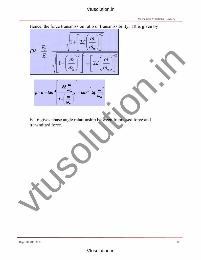
vtuso
lution
.in
Hence, the force transmission ratio or transmissibility, TR is given by
Eq. 6 gives phase angle relationship between Impressed force and
transmitted force.
−
−
=− −− nnnn11112222nnnnnnnn1111ωωωωωωωω2222ξξξξtantantantan
ωωωωωωωω1111ωωωωωωωω2222ξξξξ
tantantantanααααφφφφ
Mechanical Vibrations [10ME72]
29Dept. Of ME, ACE
Vtusolution.in
Vtusolution.in

vtuso
lution
.in
• Curves start from unity value of transmissibility pass through
unit value of transmissibility at (ω / ωn ) = and after that they
Tend to zero as (ω / ωn ) → .
Mechanical Vibrations [10ME72]
30Dept. Of ME, ACE
Vtusolution.in
Vtusolution.in

vtuso
lution
.in
• Response plot can be divided into three regions depending on
the control of spring, damper and mass.
• When (ω / ωn ) is large, it is mass controlled region. Damping
in this region deteriorates the performance of machine.
• When (ω / ωn ) is very small, it is spring controlled region.
• When (ω / ωn ) ranges from 0.6 to , it is damping controlled
region.
• For effective isolation (ω / ωn ) should be large. It means it will
have spring with low stiffness (hence large static deflections).
Motion Transmissibility
Motion transmissibility is the ratio of steady state amplitude of mass m (X)
to the steady amplitude (Y) of the supporting base.
The equations are same as that of force transmissibility. Thus the frequency
response and phase angle plots are also the same.
Problem 1
A 75 kg machine is mounted on springs of stiffness k=11.76×10⁶ N/m with a
damping factor of 0.2. A 2 kg piston within the machine has a reciprocating
motion with a stroke of 0.08 m and a speed of 3000 cpm. Assuming the
motion of the piston to be harmonic, determine the amplitude of vibration of
machine and the vibratory force transmitted to the foundation.
Solution:
Given: M = 75 kg, ξ = 0.2, mo = 2 kg, stroke = 0.08 m, N = 3000 cpm, X = ?,
FT = ?.
2222nnnn22222222nnnn2222nnnnωωωωωωωω2222ξξξξωωωω
ωωωω1111
ωωωωωωωω2222ξξξξ1111
YYYYXXXX
+
−
+
=
−
−
=− −− nnnn11112222nnnnnnnn1111ωωωωωωωω2222ξξξξtantantantan
ωωωωωωωω1111ωωωωωωωω2222ξξξξ
tantantantanααααφφφφ
Mechanical Vibrations [10ME72]
31Dept. Of ME, ACE
Vtusolution.in
Vtusolution.in

vtuso
lution
.in
Using the above eq. X = 1.25 mm (Solution)
Using the above eq. FT = 2078 N (Solution)
rad/srad/srad/srad/s12512512512575757575
1010101011.7611.7611.7611.76mmmmkkkkωωωω
5555nnnn =×
==
rad/srad/srad/srad/s314.16314.16314.16314.166060606030003000300030002222ππππωωωω =
×=
mmmm0.040.040.040.042222
0.080.080.080.08eeee2.512.512.512.51ωωωωωωωωnnnn ===
2222nnnn22222222nnnn nnnnooooωωωωωωωω2222ξξξξωωωω
ωωωω1111
ωωωωωωωω
MMMMeeeemmmm
XXXX
+
−
=
2
NNNN7900790079007900eeeeωωωωmmmmFFFF 2222oooooooo ==
Mechanical Vibrations [10ME72]
32Dept. Of ME, ACE
Vtusolution.in
Vtusolution.in

vtuso
lution
.in
Solution by Complex Algebra Here steady state solution is obtained for a system subjected to constant
excitation force using complex algebra
Let the harmonic forcing function be represented by in complex form as
Now the equation of motion becomes
Actual excitation is given by real part of F(t), the response will also
be given by real part of x(t), where x(t) is a complex quantity
satisfying the differential equation 1.
Assuming a particular solution as
Substituting eq. 3 in eq. 2
Multiplying the numerator and denominator of eq.4 by
And separating real and imaginary parts
1sin −−−=++ tFkxxcxm o ω&&&
( ) ttttiiiiooooeeeeFFFFttttFFFF ω=
2−−−=++ ttttiiiiooooeeeeFFFFkxkxkxkxxxxxccccxxxxmmmm ω&&&
( ) 3−−−= tiωXeXeXeXettttxxxx pppp( )
4444icicicicωωωωmmmmωωωωkkkk
FFFFXXXX 2222oooo −−−+−
=
( )[ ]icicicicωωωωmmmmωωωωkkkk 2222 −−
Mechanical Vibrations [10ME72]
33Dept. Of ME, ACE
Vtusolution.in
Vtusolution.in
vtuso
lution
.in
Multiplying and dividing the above expression by
Thus the steady state solution becomes
The real part of the above equation 8 gives the steady state
response
Dividing the numerator and denominator of this eq. by k
( ) ( )5555
ωωωωccccmmmmωωωωkkkkccccωωωωiiii
ωωωωccccmmmmωωωωkkkkmmmmωωωωkkkkFFFFXXXX 22222222222222222222222222222222 2222oooo −−−
+−−
+−
−=
( ) 2222222222222222 ωωωωccccmmmmωωωωkkkk +−
( ) ( ) ( )
+−
−
+−
−
+−
= 22222222222222222222222222222222 22222222222222222222oooo ωωωωccccmmmmωωωωkkkkccccωωωωiiii
ωωωωccccmmmmωωωωkkkkmmmmωωωωkkkk
ωωωωccccmmmmωωωωkkkkFFFFXXXX
( )6666eeee
ωωωωccccmmmmωωωωkkkkFFFFXXXX iiiiφφφφ2222222222222222oooo −−−
+−
= −
7777mmmmωωωωkkkkccccωωωωtantantantanφφφφwhere,where,where,where, 22221111 −−−
−
= −
( )( ) 8888eeee
ωωωωccccmmmmωωωωkkkkFFFFxxxx φφφφ----ttttiiii2222222222222222oooopppp −−−
+−
= ω
( )
( )9999
ωωωωccccmmmmωωωωkkkkφφφφωtωtωtωtcoscoscoscosFFFFxxxx 2222222222222222oooopppp −−−
+−
−=
Mechanical Vibrations [10ME72]
Vtusolution.in
Vtusolution.in

vtuso
lution
.in
Problem 1
A torsional system consists of a disc of mass moment of inertia J = 10 kg-
m2, a torsional damper of damping coefficient c = 300 N-m-s/rad, and steel
shaft of diameter 4 cm and length 1 m (fixed at one end and attached to the
disc at the other end). A steady angular oscillation of amplitude 2o is
observed when a harmonic torque of magnitude 1000 N-m is applied to the
disc. (a) Find the frequency of the applied torque, (b) find the maximum
torque transmitted to the support. Assume modulus of rigidity for the steel
rod to be 0.83×10¹¹ N/m2.
Solution:
Given: J = 10 kg-m2, c = 300 N-m-s/rad, l = 1 m, d = 4 cm,
Θ = 2o, To = 1000 N-m, G = 0.83×10¹¹ N/m
2, ω = ?, Tmax=?
Stiffness of the shaft is given by
( )[ ] ( )[ ]2222nnnnωωωωωωωω2222ξξξξ22222222nnnnωωωωωωωω1111 kkkkooooFFFFXXXX+−
=
radradradradmmmmNNNN20860208602086020860
3232323211110.040.040.040.04ππππ101010100.830.830.830.83
LLLLGIGIGIGI
θθθθTTTTkkkk
444411111111pppptttt −=×
×××===
rad/srad/srad/srad/s45.6745.6745.6745.6710101010
20860208602086020860JJJJkkkkωωωω ttttnnnn ===
( )[ ] ( )[ ]2222nnnnωωωωωωωω2222ξξξξ22222222nnnnωωωωωωωω1111 kkkkooooFFFFXXXX+−
=
( )[ ] ( )[ ]2222nnnnωωωωωωωω2222ξξξξ22222222nnnnωωωωωωωω1111 ttttkkkkooooTTTTθθθθ+−
=
0.035rad0.035rad0.035rad0.035rad180180180180
ππππ2222radiansradiansradiansradiansininininθθθθ =×
=
1.3691.3691.3691.3690.0350.0350.0350.03520860208602086020860
1000100010001000θθθθkkkk
TTTTttttoooo =×
=
34Dept. Of ME, ACE
Vtusolution.in
Vtusolution.in

vtuso
lution
.in
( ) 2222nnnn222222222222ωωωωωωωωrrrrwhere,where,where,where,1.8761.8761.8761.876rrrr4444ξξξξrrrr1111 ==+−
0.3280.3280.3280.32845.6745.6745.6745.67101010102222300300300300
2J2J2J2Jωωωωccccξξξξ nnnn =
××==
00000.8760.8760.8760.8761.569r1.569r1.569r1.569rrrrr 2222 =−−
1.4161.4161.4161.416ωωωωωωωωnnnn = rad/srad/srad/srad/s64.6864.6864.6864.68ωωωω =
2222nnnn22222222nnnn2222nnnnooootrtrtrtrωωωωωωωω2222ξξξξωωωω
ωωωω1111
ωωωωωωωω2222ξξξξ1111
TTTTTTTT
+
−
+
= mmmm1000N1000N1000N1000NTTTTtrtrtrtr −=
Mechanical Vibrations [10ME72]
35Dept. Of ME, ACE
Vtusolution.in
Vtusolution.in

vtuso
lution
.in
Vibration Measuring Instruments
Need for vibration measuring instruments
1.To detect shifts in the natural frequencies – could indicate a possible
failure or need for maintenance
2.To select operational speeds to avoid resonance
3.Theoretically estimated values may be different from the actual
values due to assumptions.
4.To design active vibration isolation systems
5.To validate the approximate model
6.To identify the system in terms of mass, stiffness and damper.
When a transducer is used in conjunction with another device to measure
vibrations it is called vibration pickup.
Commonly used vibration pickups are seismic instruments.
If the seismic instrument gives displacement of the vibrating body – It is
known as VIBROMETER.
If the seismic instrument gives velocity of the vibrating body – It is known
as VELOMETER.
If the seismic instrument gives acceleration of the vibrating body – It is
known as ACCELEROMETER.
SEISMIC INSTRUMENT
Mechanical Vibrations [10ME72]
UNIT - 5
VIBRATION MEASURING INSTRUMENTS
1Dept. Of ME, ACE
Vtusolution.in
Vtusolution.in

vtuso
lution
.in
Vibrating body is assumed to have a Harmonic Motion given by
Eq. of motion for the mass m can be written as
Defining relative displacement as
Substituting this value of x in equation 2
Steady state solution of eq. 4 is given by
1−−−= ttttYsinYsinYsinYsinyyyy ω
( ) ( ) 22220000yyyyxxxxkkkkyyyyxxxxccccxxxxmmmm −−−=−+−+ &&&&
zzzzyyyyxxxxor,or,or,or,3333yyyyxxxxzzzz
+=
−−−=
4444------------ttttYsinYsinYsinYsinmmmmωωωωkzkzkzkzzzzzcccczzzzmmmmyyyymmmmkzkzkzkzzzzzcccczzzzmmmm 2222 ω=++
−=++
&&&
&&&&&
( )φφφφωtωtωtωtZsinZsinZsinZsinzzzz −=
[ ] ( )
−=
−
=
=
+−
=
+
−
=
−−
2
1
2
n
n1
n222
2
2
n
22
n
2
n
r1
r2ξtan
ω
ω1
ω
ω2ξ
tanφ
ω
ωrwhere
r2ξr1
r
ω
ω2ξ
ω
ω1
ω
ω
Y
Z
Mechanical Vibrations [10ME72]
2Dept.Of ME, ACE
Vtusolution.in
Vtusolution.in

vtuso
lution
.in
The frequency response plot is shown in the fig. The type of instrument is
determined by the useful range of frequency
The phase angle plot shown below indicates the phase lag of the seismic
mass with respect to vibrating base of machine
0 1 2 3 4
0
1
2
3
4
Accele
rom
ete
r
Vib
rom
ete
r
an
d
Ve
lom
ete
r
ζ = 0 .0
ζ = 0 .1
ζ = 0 .2
ζ = 0 .3
ζ = 0 .4
ζ = 0 .5
ζ = 0 .7 0 7
ζ = 1
Z/Y
ω / ωn ( r )
0 1 2 3 4 5
0
2 0
4 0
6 0
8 0
1 0 0
1 2 0
1 4 0
1 6 0
1 8 0
ξ = 1 .0
ξ = 0 .7 0 7ξ = 0 .5
ξ = 0 .2
ξ = 0 .1
ξ = 0
Pha
se
an
gle
, φ
ω /ωr ( r )
Mechanical Vibrations [10ME72]
33Dept.Of ME, ACE
Vtusolution.in
Vtusolution.in
vtuso
lution
.in
Vibrometers Used for measurement of displacement of vibrating body.
It means when Z / Y ~ 1, the observed reading on the scale directly gives the
displacement of the vibrating body. For this to happen r = ω / ωn ≥ 3.
Thus when r = ω / ωn ≥ 3, Z / Y ~ 1, but there is a phase lag. Z lags behind Y
by an angle φ or by time lag of t = φ / ω. This time lag is not important if
the input consists of single harmonic component.
Thus for vibrometers the range of frequency lies on the right hand side of
frequency response plot. It can also be seen from the plot a better
approximation can be obtained if ξ is less than 0.707.
Also for fixed value of ω, and for the value of ωn
must be small. It means mass must be very large and stiffness must be small.
This results in bulky instrument which may not be desirable in many
applications.
Accelerometer
Accelerometer measures the acceleration of a vibrating body.
They are widely used for measuring acceleration of vibrating bodies and
earthquakes. Integration of acceleration record provides displacement and
velocity.
( )φφφφωtωtωtωtZsinZsinZsinZsinzzzz −=
[ ] ( ) Y
Z1
r2ξr1
r222
2
==
+−ttttYsinYsinYsinYsinyyyy ω=
[ ] ( )
[ ] ( ) 2222nnnn22222222 222222222222 222222222222 2222ωωωω
YYYYωωωωZZZZ Y,Y,Y,Y,rrrrZZZZthenthenthenthen
1111rrrr2222ξξξξrrrr1111
1111rrrr2222ξξξξrrrr1111
rrrrYYYYZZZZ
==
=
+−
+−
=
Mechanical Vibrations [10ME72]
4Dept. Of ME, ACE
Vtusolution.in
Vtusolution.in
vtuso
lution
.in
The expression is equal to the acceleration amplitude of the
Vibrating body. The amplitude recorded by the instrument is proportional to
the acceleration of vibrating body since ωn is constant for the instrument.
For an accelerometer the ratio << 1 and the range of operation lies
on the extreme left hand side of the frequency
response curve.
Since << 1, the natural frequency must be high. That is mass
must be as low as possible. Thus the instrument is small in size and is
preferred in vibration measurement.
Frequency ratio, r should be between 0 and 0.6
Damping ratio, ξ , should be less than 0.707
Problem 1 The static deflection of the vibrometer mass is 20 mm. The
instrument when attached to a machine vibrating with a frequency of 125
cpm records a relative amplitude of 0.03 cm. Determine (a) the amplitude of
vibration (b) the maximum velocity of vibration (c) the maximum
acceleration.
Solution:
Given: dst = 20 mm, f = 125 cpm, Z = 0.03 cm, Y = ?,
Vmax = ?, a = ?, ξ = 0.0
YYYYωωωω 2222
0.590.590.590.59ωωωωωωωωrrrr
rad/srad/srad/srad/s13.0913.0913.0913.0960606060NNNN2222ππππωωωωrad/srad/srad/srad/s22.1522.1522.1522.150.020.020.020.02
9.819.819.819.81ddddggggωωωω nnnn ststststnnnn==
=====
[ ] ( )0000ξξξξasasasasrrrr1111
rrrrrrrr2222ξξξξrrrr1111
rrrrYYYYZZZZ 22222222222222222222 2222
=−
=
+−
=
2222222222222222
cm/scm/scm/scm/s95.9595.9595.9595.95YYYYωωωωononononAcceleratiAcceleratiAcceleratiAcceleratiMaxMaxMaxMaxcm/scm/scm/scm/s0.7330.7330.7330.733YYYYωωωωVelocityVelocityVelocityVelocityMaxMaxMaxMax
0.56cm0.56cm0.56cm0.56cm0.5340.5340.5340.5340.030.030.030.03YYYY
0.5340.5340.5340.5340.590.590.590.5911110.590.590.590.59
YYYYZZZZ
==
==
==
=−
=
Mechanical Vibrations [10ME72]
5Dept. Of ME, ACE
Vtusolution.in
Vtusolution.in
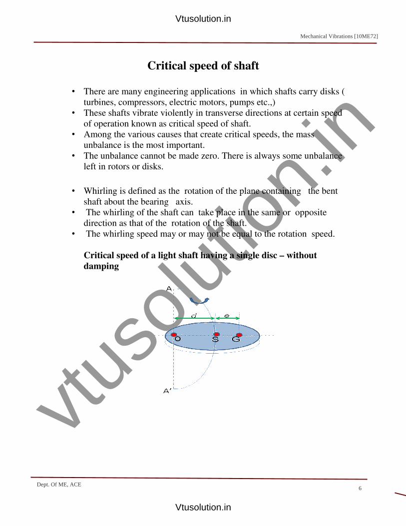
vtuso
lution
.in
Critical speed of shaft
• There are many engineering applications in which shafts carry disks (
turbines, compressors, electric motors, pumps etc.,)
• These shafts vibrate violently in transverse directions at certain speed
of operation known as critical speed of shaft.
• Among the various causes that create critical speeds, the mass
unbalance is the most important.
• The unbalance cannot be made zero. There is always some unbalance
left in rotors or disks.
• Whirling is defined as the rotation of the plane containing the bent
shaft about the bearing axis.
• The whirling of the shaft can take place in the same or opposite
direction as that of the rotation of the shaft.
• The whirling speed may or may not be equal to the rotation speed.
Critical speed of a light shaft having a single disc – without
damping
Mechanical Vibrations [10ME72]
6Dept. Of ME, ACE
Vtusolution.in
Vtusolution.in

vtuso
lution
.in
Consider a light shaft carrying a single disc at the centre in deflected
position. ‘S’ is the geometric centre through which centre line of shaft
passes. ‘G’ is centre of gravity of disc. ‘O’ intersection of bearing centre
line with the disc ‘e’ is distance between c.g. ‘G’ and the geometric centre
‘S’. ‘d’ is displacement of the geometric centre ‘S’ from the un deflected
position ‘O’. ‘k’ is the stiffness of the shaft in the lateral direction.
The forces acting on the disc are
- Centrifugal force ‘mω2(d+e)’ acts radially outwards at ‘G’
- Restoring force ‘kd’ acts radially inwards at ‘S’
- For equilibrium the two forces must be equal and act along the
same line
• Deflection ‘d’ tends to infinity when ω = ωn
• ‘d’ is positive below the critical speed, the disc rotates with
heavy side outside when ω < ωn
• ‘d’ is negative above the critical speed, the disc rotates with
light side outside when ω > ωn
• When ω >> ωn, ‘d → - e’ , which means point ‘G’ approaches
point ‘O’ and the disc rotates about its centre of gravity.
( )
( )2
r1
er
ω
ω1
eω
ω
mωk
emωd
1kredmω
2
2
2
n
2
n
2
2
2
−−−−
=
−
=−
=
−−−=+
Mechanical Vibrations 10ME72[
7Dept. Of ME, ACE
Vtusolution.in
Vtusolution.in

vtuso
lution
.in
Problem 1
A rotor having a mass of 5 kg is mounted midway on a 1 cm shaft supported
at the ends by two bearings. The bearing span is 40 cm. Because of certain
manufacturing inaccuracies, the centre of gravity of the disc is 0.02 mm
away from the geometric centre of the rotor. If the system rotates at 3000
rpm find the amplitude of steady state vibrations and the dynamic force
transmitted to the bearings. Assume the rotor to be simply supported. Take E
= 1.96×10¹¹
N/m2.
Solution:
Given: m = 5 kg, d = 1 cm, l = 40 cm, e = 0.02 mm,
N = 3000 rpm, E = 1.96×10¹¹
N/m2 , d = ?, Simply supported
In the above eq. e and ω are known, ωn has to be found out in order to find
d. To find ωn, stiffness has to be determined.
For a simply supported shaft the deflection at the mid point is given by the
following equation.
−
=2
n
2
n
ω
ω1
ω
ω
e
d
N/m720000.464
0.01π101.9648
l
48EI
δ
mgk,
48EI
mglδ
3
411
3
3
=×
××××====
Mechanical Vibrations [10ME72]
8Dept. Of ME, ACE
Vtusolution.in
Vtusolution.in
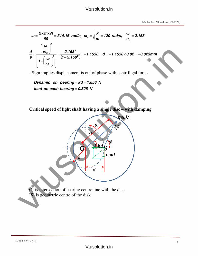
vtuso
lution
.in
- Sign implies displacement is out of phase with centrifugal force
Critical speed of light shaft having a single disc – with damping
O’ is intersection of bearing centre line with the disc
’S’ is geometric centre of the disk
2.168ω
ωrad/s,120
m
kω rad/s,314.16
60
Nπ2ω
n
n ====××
=
( )0.023mm0.021.1558d1.1558,
2.1681
2.168
ω
ω1
ω
ω
e
d2
2
2
n
2
n−=×−=−=
−=
−
=
N0.828bearingeachonload
N1.656kdbearingonDynamic
=
==
Mechanical Vibrations [10ME72]
9Dept. Of ME, ACE
Vtusolution.in
Vtusolution.in

vtuso
lution
.in
‘G’ is centre of gravity of disc
The forces acting on the disc are
1. Centrifugal force at G along OG produced
2. Restoring force kd at S along SO
3. Damping force cωd at S in a direction opposite to velocity at S
4. The points O,S and G no longer lie on straight line
Let,
OG = a,SG = e,OS = d,∟GOS = α ∟GSA = φ
From the geometry
Eliminating a and α from equations 3 and 4 with the help of equations 1 and
2
2ecosφdacosα
1esinφasinα
−−−+=
−−−=
40asinαmωdcω
0,Y
30amωkd
0,X
2
2
−−−=+−
=
−−−=+−
=
∑
∑
( )
( ) 60esinφmωdcω
50ecosφdmωkd2
2
−−−=+−
−−−=++−
Mechanical Vibrations[10ME72]
10Dept. Of ME, ACE
Vtusolution.in
Vtusolution.in

vtuso
lution
.in
Squaring and adding the equations 7 and 8
From the curves or the equation it can be seen that (Discussions of speeds
above and below critical speed)
(a) Φ ~ 0 when ω << ωn (Heavy side out)
(b) 0 < φ < 90° when ω < ωn (Heavy side out)
8emω
dcωsinφeq.6From
7emω
dmωkdcosφeq.5From
2
2
2
−−−=
−−−−
=
( ) ( )222
2
cωmωk
mω
e
d
+−
=
( ) ( )9
r2ξr1
r
ω
ω2ξ
ω
ω1
ω
ω
e
d222
2
2
n
2
n
2
n−−−
+−
=
+
−
=
10r1
r2ξtan
ω
ω1
ω
ω2ξ
tanφ2
1
2
n
n1 −−−−
=
−
= −−
Mechanical Vibrations [10ME72]
11Dept. Of ME, ACE
Vtusolution.in
Vtusolution.in

vtuso
lution
.in
(c) Φ = 90° when ω = ωn
(d) 90° < Φ < 180° when ω > ωn (Light side out)
Mechanical Vibratiosn [10ME72]
12Dept. Of ME, ACE
Vtusolution.in
Vtusolution.in

vtuso
lution
.in
(e) Φ ~ 180° when ω >> ωn, (Light side out, disc rotates about its
centre of gravity)
Critical speed of shaft may be placed above or below the operating speed.
1. If the unit is to operate at high speeds, that do not vary widely, the critical
speed may be below the operating speed, and the shaft is then said to be
flexible.
2 In bringing the shaft up to the operating speed, the critical speed must be
passed through. If this is done rapidly, resonance conditions do not have
chance to build up.
3. If the operating speed is low or if speeds must vary through wide ranges,
the critical speed is placed over the operating speed and the shaft is said to
be rigid or stiff.
4. Generally the running speed must at least 20% away from the critical
speed.
Problem 1
A disk of mass 4 kg is mounted midway between the bearings
Which may be assumed to be simply supported. The bearing span is 48 cm.
The steel shaft is 9 mm in diameter. The c.g. of the disc is displaced 3 mm
from the geometric centre. The equivalent viscous damping at the centre of
Mechanical Vibrations [10ME72]
13Dept. Of ME, ACE
Vtusolution.in
Vtusolution.in

vtuso
lution
.in
the disc- shaft may be taken as 49 N-s/m. If the shaft rotates at 760 rpm, find
the maximum stress in the shaft and compare it with the dead load stress in
the shaft when the shaft is horizontal. Also find the power required to drive
the shaft at this speed. Take E = 1.96 × 10¹¹
N/m2.
Solution:
Given: m = 4kg, l = 48 cm, e = 3 mm, c = 49 N-s/m, N = 760rpm
E = 1.96 × 10¹¹
N/m2, smax = ?. Dia = 9 mm, E = 1.96 × 10
11 N/m
2.
d = 0.017 m (solution)
The dynamic load on the bearings is equal to centrifugal force of the disc
which is equal to the vector sum of spring force and damping force.
The total maximum load on the shaft under dynamic conditions is the sum of
above load and the dead load.
The load under static conditions is
The maximum stress, due to load acting at the centre of a simply supported
shaft is
0.074km2
cξ
79.5rad/s60
2ππω
82.8rad/sm
kω
27400N/ml
48EIk
n
3
==
==
==
==
2
n
2
n
2
n
ω
ω2ξ
ω
ω1
ω
ω
e
d
+
−
=
( ) ( ) ( ) 470NcωkddcωkdF2222
dy =+=+=
( ) 509.2N9.814470Fmax =×+=
39.2N9.814Fs =×=
Mechanical Vibrations [10ME72]
14Dept. Of ME, ACE
Vtusolution.in
Vtusolution.in
vtuso
lution
.in
The total maximum stress under dynamic conditions
Maximum stress under dead load
--------------------------------------------------------------------------------------------
F10168diaπ24
64diaFl
2I
diaMs 4
4×=
×××
××=
×
×=
28
max
4
max N/m108.55F10168s ×=××=
274
max N/m106.5939.210168s ×=××=
( )
90W60
NT2πPower
m1.125NddcωTtorqueDamping
==
−===
Mechanical Vibrations [10ME72]
15Dept. Of ME, ACE
Vtusolution.in
Vtusolution.in

vtuso
lution
.in
1
Unit - 6
Vibrations of Two Degree of Freedom Systems
Dr. T. Jagadish. Professor for Post Graduation, Department of Mechanical Engineering,
Bangalore Institute of Technology, Bangalore
Introduction
A two degree of freedom system is one that requires two coordinates to completely describe
its equation of motion. These coordinates are called generalized coordinates when they are
independent of each other. Thus system with two degrees of freedom will have two equation of
motion and hence has two frequencies.
A two degree freedom system differs from a single degree of freedom system in that it has
two natural frequencies and for each of these natural frequencies there correspond a natural state of
vibration with a displacement configuration known as NORMAL MODE. Mathematical terms
related to these quantities are known as Eigen values and Eigen vectors. These are established from
the two simultaneous equation of motion of the system and posses certain dynamic properties
associated.
A system having two degrees of freedom are important in as far as they introduce to the
coupling phenomenon where the motion of any of the two independent coordinates depends also on
the motion of the other coordinate through the coupling spring and damper. The free vibration of two
degrees of freedom system at any point is a combination of two harmonics of these two natural
frequencies.
Under certain condition, during free vibrations any point in a system may execute harmonic
vibration at any of the two natural frequencies and the amplitude are related in a specific manner and
the configuration is known as NORMALMODE or PRINCIPAL MODE of vibration. Thus system
with two degrees of freedom has two normal modes of vibration corresponding two natural
frequencies.
Free vibrations of two degrees of freedom system:
Consider an un-damped system with two degrees of freedom as shown in Figure 6.1a, where
the masses are constrained to move in the direction of the spring axis and executing free vibrations.
The displacements are measured from the un-stretched positions of the springs. Let x1 and x2 be the
displacement of the masses m1 and m2 respectively at any given instant of time measured from the
Mechanical Vibrations [10ME72]
UNIT - 6
SYSTEMS WITH TWO DEGREES OF FREEDOMS
Dept. Of ME, ACE
Vtusolution.in
Vtusolution.in

vtuso
lution
.in
2
equilibrium position with x2 > x1. Then the spring forces acting on the masses are as shown in free
body diagram in Figure 6.1b
(a) (b)
Figure 6.1
Based on Newton’s second law of motion ∑ƒ =
For mass m1
for mass (2)
The solution for x1 and x2 are obtained by considering that they can have harmonic vibration under
steady state condition. Then considering the case when the mass m1 execute harmonic vibration at
frequency ω1 and the mass m2 execute harmonic vibration at frequency ω2 then we have
x1 = X1 sin ω1t, and x2 = X2 sin ω2t ----------- (3)
Where X1 and X2 are the amplitudes of vibrations of the two masses under steady state conditions.
Substituting equation (3) into equation (1) we have
- m1ω12X1 sin ω1t + (k1 + k2) X1 sin ω1t = k2 X2 sin ω2t
Therefore X1 = k2 sinω2t
X2 (k1 + k2 ) – mω12 sinω1t
Since X1 and X2 are the amplitude of two harmonic motions, their ratio must be constant and
independent of time. Therefore sinω2t / sinω1t = C a constant.
.. m x
.. m1 x1 + k1 x1 - k2x2 + k2x1 = 0
.. m1 x1 + (k1 + k2) x1 = k2x2 ------------ (1)
= ..
m1 x1 - k1 x1 + k2(x2 –x1)
.. m2 x2 + k3 x2 + k2x2 - k2x1 = 0
.. m2 x2 + (k2 + k3) x2 = k2x1 ------------ (2)
= ..
m2 x2 - k3 x2 - k2(x2 –x1)
k1x1
k2(x2 - x1)
k3x2
..
m1x1
..
m2x2
m1
m2 m
k2
k1
x1
x2
k3
Mechanical Vibrations[10ME72]
Dept. Of ME, ACE
Vtusolution.in
Vtusolution.in
vtuso
lution
.in
3
Consider if C > 1. Then at time t = π/2ω1 , sinω1t will be sinω1 x π/2ω1 = sin π/2 = 1
Therefore sinω2t / sinω1t > 1 or sinω2t > 1 which is impossible. Hence C > 1 is not possible.
Similarly it can be shown that C < 1 is also not possible. Thus the only possibility is that C = 1
Hence sinω2t / sinω1t = 1 which is only possible if ω2 = ω1 = ω. Hence the two harmonic motion
have to be of the same frequency. Thus the solution of equation (1) and (2) can be
x1 = X1 sin ωt, and x2 = X2 sin ωt ----------- (4)
------------------ (5)
Substitute equation (4) and (5) into the equation (1) and (2)
- m1ω2X1 sin ωt + (k1 + k2) X1 sin ωt = k2 X2 sin ωt ----------------- (6)
- m2 ω2X2 sin ωt + (k2 + k3) X2 sin ωt = k2 X1 sin ωt. ----------------- (7)
Canceling the common term sin ωt on both the sides and re arranging the terms we have from
equation (6)
X1/X2 = k2 / (k1 + k2 – m1ω2) ---------------- (8)
X1/X2 = [(k2 + k3) – m2ω2] / k2 ----------- (9)
Thus equating equation (8) and (9) we have
X1/X2 = k2 / (k1 + k2 – m1ω2) = [(k2 + k3) – m2ω
2] / k2 -------------- (10)
Cross multiplying in equation (10) we have
(k1 + k2 – m1ω2) (k2 + k3 – m2ω
2) = k2
2 on simplification we get
m1m2 ω4 – [m1 (k2 + k3) + m2 (k1 + k2)] ω
2 + [k1k2 + k2k3 + k3k1] = 0 ---------- (11)
The above equation (11) is quadratic in ω2 and gives two values of ω
2 and therefore the two positive
values of ω correspond to the two natural frequencies ωn1 and ωn2 of the system. The above equation
is called frequency equation since the roots of the above equation give the natural frequencies of the
system.
Now considering m1 = m2 = m and k1 = k3 = k
Then the frequency equation (11) becomes
m2ω
4 – 2m (k + k2) ω
2 + (k
2 + 2kk2) = 0 ------------------ (12)
Let: ω2 = λ ∴λ
2 = ω
4, ∴ m
2 λ
2 – 2 m (k + k2) λ + (k
2 + 2kk2) = 0 ------------------ (13)
The roots of the above equation (13) are as follows: Let a = m2, b = -2 m (k + k2); c = (k
2 + 2kk2)
∴ λ1,2 = [- b ± √(b2 – 4ac)] / 2a
λ1,2 = [- (-2m) (k + k2) ± √[-2m (k+k2)]2 – 4 (m
2) (k
2 + 2kk2)]/2m
2
= [+ 2m (k +k2)] / 2m2 ± [√4m
2[(k
2 + k2
2 + 2 kk2) – (k
2 + 2kk2)]/4m
4 = (k+ k2) /m ± √(k2
2/m
2)
= (k +k2) /m ± k2/m
.. x1= - ω
2X1 sin ωt
.. x2= - ω
2X2 sin ωt
Mechanical Vibrations [10ME72]
Dept. Of ME, ACE
Vtusolution.in
Vtusolution.in

vtuso
lution
.in
4
Thus λ1 = (k + k2) /m – k2 / m = k/m. Then ωn12 = K/m ∴∴∴∴ωωωωn1 = √√√√(k/m) ----------------- (14)
and ∴λ2 = (k + 2k2) /m Thus ωn22 = (k + 2k2) /m. Then ∴∴∴∴ωωωωn2 = √√√√[(k + 2k2) /m] --- (15)
ωn1 is called the first or fundamental frequency or 1st mode frequency, ωn2 is called the second or 2
nd
mode frequency. Thus the number of natural frequencies of a system is equal to the number of
degrees of freedom of system.
Modes Shapes: From equation (10) we have X1/X2 = k2/(k+k2) -mω2 = (k2 + k) - mω
2/k2 ---(16)
Substitute ωn1 = √(k/m) in any one of the above equation (16).
(X1/X2)ωn1 = k2 / (k+ k2 – m(k/m)) or ((k2 + k) – m(k/m))/k2 = k2/k2 = 1
(X1/X2)ωn1 = 1 ----------------- (17)
Similarly substituting ωn2 = √[(k + 2k2) /m] in any one of the above equation (16).
(X1/X2)ωn2 = k2 / (k + k2 – m(k+ 2k2)/m) or ((k2 + k) – m(k+ 2k2)/m))/k2 = - k2/k2 = -1
(X1/X2)ωn2 = -1 ----------------- (18)
The displacements X1 and X2 corresponding to the two natural frequency of the system can be
plotted as shown in Figure 6.2, which describe the mode in which the masses vibrate. When the
system vibrates in principal mode the masses oscillate in such a manner that they reach maximum
displacements simultaneously and pass through their equilibrium points simultaneously or all
moving parts of the system oscillate in phase with one frequency. Since the ratio X1/X2 is important
rather than the amplitudes themselves, it is customary to assign a unit value of amplitude to either X1
or X2. When this is done, the principal mode is referred as normal mode of the system.
(a) (b) (c)
Figure – 6.2
ωn1 = √(k/m) ωn2 = √[(k + 2k2) /m]
1st Mode 2
nd Mode
m1
m2
k3
k2
k1
x1
x2
x1 = 1
x2 = 1
Node
x1 = 1
x2 = -1
Mechanical Vibrations [10ME72]
Dept.Of ME, ACE
Vtusolution.in
Vtusolution.in

vtuso
lution
.in
5
It can be observed from the figure – 6.2b when the system vibrates at the first frequency, the
amplitude of two masses remain same. The motion of both the masses are in phase i.e., both the
masses move up or down together, the length of the middle spring remains constant, this spring
(coupling spring) is neither stretched nor compressed. It moves rigid bodily with both the masses and
hence totally ineffective as shown in Figure 6.3a. Even if the coupling spring is removed the two
masses will vibrate as two single degree of freedom systems with ωn = √(K/m).
When the system vibrates at the second frequency the displacement of the two masses have
the same magnitude but with opposite signs. Thus the motions of m1 and m2 are 1800 out of phase,
the midpoint of the middle spring remains stationary for all the time. Such a point which experiences
no vibratory motion is called a node, as shown in Figure 6.3b which is as if the middle of the
coupling spring is fixed
When the two masses are given equal initial displacements in the same direction and
released, they will vibrate at first frequency. When they are given equal initial displacements in
opposite direction and released they will vibrate at the second frequency as shown in Figures 6.3a
and 6.3b
(a) (b)
Figure – 6.3
ωn1 = √(k/m) ωn2 = √[(k + 2k2) /m]
1st Mode 2
nd Mode
If unequal displacements are given to the masses in any direction, the motion will be superposition
of two harmonic motions corresponding to the two natural frequencies.
m1
m2
k3
k1
x1
x2
m1
m2
k3
k1
x1
x2
= - T1
θ
Mechanical Vibrations [10ME72]
Dept Of ME, ACE
Vtusolution.in
Vtusolution.in
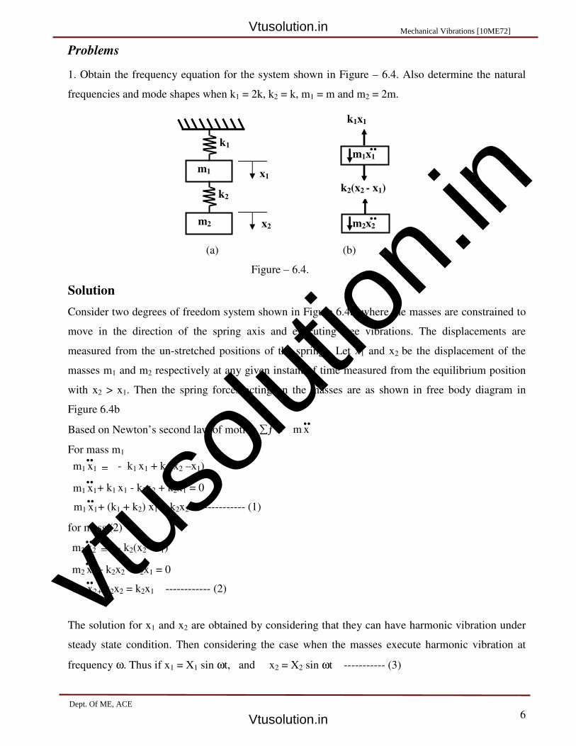
vtuso
lution
.in
6
Problems
1. Obtain the frequency equation for the system shown in Figure – 6.4. Also determine the natural
frequencies and mode shapes when k1 = 2k, k2 = k, m1 = m and m2 = 2m.
(a) (b)
Figure – 6.4.
Solution
Consider two degrees of freedom system shown in Figure 6.4a, where the masses are constrained to
move in the direction of the spring axis and executing free vibrations. The displacements are
measured from the un-stretched positions of the springs. Let x1 and x2 be the displacement of the
masses m1 and m2 respectively at any given instant of time measured from the equilibrium position
with x2 > x1. Then the spring forces acting on the masses are as shown in free body diagram in
Figure 6.4b
Based on Newton’s second law of motion ∑ƒ =
For mass m1
for mass (2)
The solution for x1 and x2 are obtained by considering that they can have harmonic vibration under
steady state condition. Then considering the case when the masses execute harmonic vibration at
frequency ω. Thus if x1 = X1 sin ωt, and x2 = X2 sin ωt ----------- (3)
k1x1
k2(x2 - x1)
..
m1x1
..
m2x2
m1
m2
k2
k1
x1
x2
.. m x
.. m1 x1 + k1 x1 - k2x2 + k2x1 = 0
.. m1 x1 + (k1 + k2) x1 = k2x2 ------------ (1)
= ..
m1 x1 - k1 x1 + k2(x2 –x1)
.. m2 x2 + k2x2 - k2x1 = 0
.. m2 x2 + k2x2 = k2x1 ------------ (2)
= ..
m2 x2 - k2(x2 –x1)
Mechanical Vibrations [10ME72]
Dept. Of ME, ACE
Vtusolution.in
Vtusolution.in

vtuso
lution
.in
7
Then we have x1= - ω2X1 sin ωt, x2 = - ω
2 X2 sin ωt ------------------ (4)
Substitute equation (3) and (4) into the equation (1) and (2) we get
- m1ω2X1 sin ωt + (k1 + k2) X1 sin ωt = k2 X2 sin ωt ----------------- (5)
- m2 ω2X2 sin ωt + k2X2 sin ωt = k2 X1 sin ωt. ----------------- (6)
From equation (5) we have X1/X2 = k2/[(k1 + k2) – m1ω2] -------------- (7)
From equation (6) we have X1/X2 = [ k2 – m2ω2] / k2 -------------- (8)
Equating (7) and (8)
k2 / (k1 + k2 – m1ω2) = [k2 – m2ω
2] /k2
k22 = (k1 + k2 – m1ω
2) (k2 – m2ω
2)
k22 = (k1 + k2) k2 – m1ω
2 k2 – m2ω
2 (k1 + k2) + m1 m2ω
4
m1 m2 ω4 - ω
2 [m1 k2 + m2 (k1 + k2)] + k1 k2 = 0 --------------- (9)
letting ω2 = λ m1 m2 λ
2 – λ [m1k2 + m2 (k1 + k2)] + k1k2 = 0 ---------------------- (10)
Equation (10) is the frequency equation of the system which is quadratic in λ and hence the solution
is
λ = [[m1k2 + m2 (k1 + k2)] ± √ [[{m1k2 + m2(k1+k2)}2]- 4 m1 m2k1k2]] / 2m1m2
To determine the natural frequencies Given k1 = 2 k, k2 = k and m1 = m, m2 = 2m
λ = [mk + 2m (2k +k) ± √[mk + 6mk)2 – 4m 2mk
2k]] / 2m . 2m
= [7mk ± √[(7mk)2 – 4 (4m
2k
2)]] / 4m
2
= [7mk ± √(49m2k
2 – 16m
2k
2] / 4m
2
λ = [7mk ± 5.744 mk] /4m2 Thus λ1 = [7mk - 5.744 mk]/4m
2 and λ2 = [7mk + 5.744 mk] /4m
2
λ1 = ωn12 = [7 mk – 5.744 mk] /4m
2 = 1.255 mk /4m
2 = 0.3138 k/m Thus ωωωωn1 = 0.56 √√√√(k/m)
λ2 = ωn22 = [7mk + 5.744 mk] /4m
2 = 3.186 k/m. Thus ωωωωn2 = 1.784 √√√√(k/m)
Substituting the values of frequencies into the amplitude ratio equation as given by equation (7) and
(8) one can determine the mode shapes:
FOR THE FIRST MODE:
Substituting ωn12 = 0.3138 K/m into either of the equation (7) or (8) we get first mode shape:
I.e. X1/X2 = k2/[(k1 + k2) – m1ω2] -------------- (7) X1/X2 = [ k2 – m2ω
2] / k2 -------------- (8)
X1/X2 = k / [(2k + k – m ω2] = k/ [3k –m. ωn1
2]
X1/X2 = k/ [3k –2m. 0.3138k/m] = 1/(3 – 0.3138) =1/2.6862 = 0.3724
Thus we have X1/X2 = 0.3724. Then If X1 = 1, X2 = 2.6852
Mechanical Vibrations [10ME72]
Dept. Of ME, ACE
Vtusolution.in
Vtusolution.in
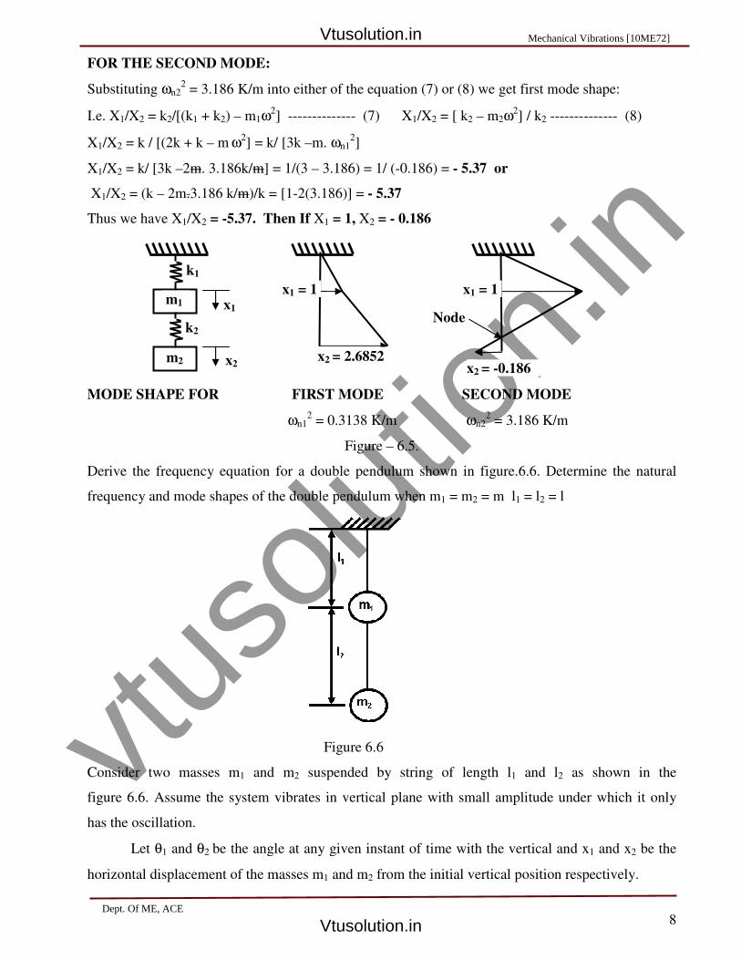
vtuso
lution
.in
FOR THE SECOND MODE:
Substituting ωn22 = 3.186 K/m into either of the equation (7) or (8) we get first mode shape:
I.e. X1/X2 = k2/[(k1 + k2) – m1ω2]
X1/X2 = k / [(2k + k – m ω2] = k/ [3k
X1/X2 = k/ [3k –2m. 3.186k/m] = 1/(3
X1/X2 = (k – 2m.3.186 k/m)/k = [1
Thus we have X1/X2 = -5.37. Then If
MODE SHAPE FOR FIRST MODE
Derive the frequency equation for a double pendulum shown in figure.6.
frequency and mode shapes of the double pendulum when m
Consider two masses m1 and m
figure 6.6. Assume the system vibrates in vertical plane with small amplitude under which it only
has the oscillation.
Let θ1 and θ2 be the angle at any given instant of time with the vertical and x
horizontal displacement of the masses m
m1
m2
k2
k1
x1
x2
= 3.186 K/m into either of the equation (7) or (8) we get first mode shape:
] -------------- (7) X1/X2 = [ k2 – m2ω2] / k2 --------------
] = k/ [3k –m. ωn12]
] = 1/(3 – 3.186) = 1/ (-0.186) = - 5.37 or
)/k = [1-2(3.186)] = - 5.37
5.37. Then If X1 = 1, X2 = - 0.186
SHAPE FOR FIRST MODE SECOND MODE
ωn12 = 0.3138 K/m ωn2
2 = 3.186 K/m
Figure – 6.5.
Derive the frequency equation for a double pendulum shown in figure.6.6. Determine the natural
frequency and mode shapes of the double pendulum when m1 = m2 = m l1 = l2 = l
Figure 6.6
and m2 suspended by string of length l1 and l
. Assume the system vibrates in vertical plane with small amplitude under which it only
be the angle at any given instant of time with the vertical and x
horizontal displacement of the masses m1 and m2 from the initial vertical position respectively.
x1 = 1
x2 = 2.6852
x1 = 1
x2 = -0.186
Node
8
= 3.186 K/m into either of the equation (7) or (8) we get first mode shape:
-------------- (8)
SECOND MODE
= 3.186 K/m
. Determine the natural
= l
and l2 as shown in the
. Assume the system vibrates in vertical plane with small amplitude under which it only
be the angle at any given instant of time with the vertical and x1 and x2 be the
om the initial vertical position respectively.
Mechanical Vibrations [10ME72]
Dept. Of ME, ACE
Vtusolution.in
Vtusolution.in
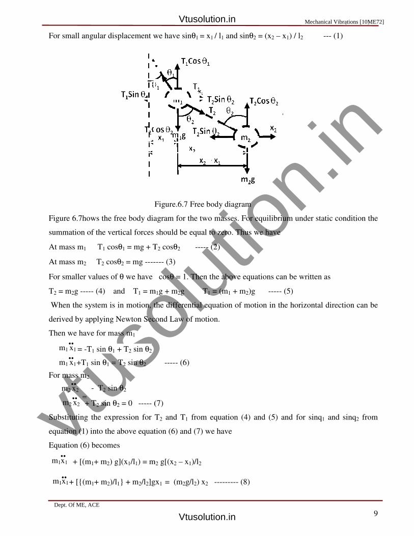
vtuso
lution
.in
For small angular displacement we have sin
Figure.6.
Figure 6.7hows the free body diagram for the two masses. For equilibrium under static condition the
summation of the vertical forces should be equal to zero. Thus we have
At mass m1 T1 cosθ1 = mg + T
At mass m2 T2 cosθ2 = mg -------
For smaller values of θ we have
T2 = m2g ----- (4) and T1 = m
When the system is in motion, t
derived by applying Newton Second Law of motion
Then we have for mass m1
For mass m2
Substituting the expression for T
equation (1) into the above equation (6) and (7) we have
Equation (6) becomes
= .. m2 x2 + T2 sin θ2 = 0 ----- (7)
- T2 sin θ2 ..
m2 x2
.. m1x1
+ [(m1+ m2) g](x1/l1) = m
+ [{(m1+ m2)/l1} + m2/l2]gx ..
m1x1
.. m1 x1 +T1 sin θ1 = T2 sin θ2
.. m1 x1 = -T1 sin θ1 + T2 sin θ2
For small angular displacement we have sinθ1 = x1 / l1 and sinθ2 = (x2 – x1) / l2
Figure.6.7 Free body diagram
hows the free body diagram for the two masses. For equilibrium under static condition the
summation of the vertical forces should be equal to zero. Thus we have
= mg + T2 cosθ2 ----- (2)
------- (3)
cosθ = 1. Then the above equations can be written as
= m1g + m2g T1 = (m1 + m2)g ----- (5)
the differential equation of motion in the horizontal direction can be
derived by applying Newton Second Law of motion.
Substituting the expression for T2 and T1 from equation (4) and (5) and for sinq
equation (1) into the above equation (6) and (7) we have
(7)
) = m2 g[(x2 – x1)/l2
gx1 = (m2g/l2) x2 --------- (8)
----- (6)
9
--- (1)
hows the free body diagram for the two masses. For equilibrium under static condition the
= 1. Then the above equations can be written as
ion of motion in the horizontal direction can be
from equation (4) and (5) and for sinq1 and sinq2 from
Mechanical Vibrations[10ME72]Mechanical Vibrations [10ME72]
Dept. Of ME, ACE
Vtusolution.in
Vtusolution.in

vtuso
lution
.in
10
Equation (7) becomes
Equations (8) and (9) represent the governing differential equation of motion. Thus assuming the
solution for the principal mode as
Substitute in (10) into equation (8) and (9) and cancelling the common term sinωt we have
[-m1ω2+{(m1+m2)/l1+m2/l2}g]A=(m2g /l2)B --(11)
[-m2ω2+(m2g/l2)]B = (m2g/l2)A ---------- (12)
From equation (11) we have
A/B=(m2g/l2)/[{(m1+m2)/l1+m2/l2}g]-m1ω2 -- (13)
From equation (12) we have
A/B = [(m2g / l2) -m2ω2] / (m2g / l2) ------ (14)
Equating equation (13) and (14) we have
A/B = (m2g/l2)/[{(m1+m2)/l1 + m2/l2}g-m1ω2] = [(m2g/l2) -m2ω
2]/(m2g/l2)
[{(m1+ m2)/l1+m2/l2}g-m1ω2][(m2g/l2) -m2ω
2] = (m2g / l2)
2 ------- (15)
Equation (15) is a the quadratic equation in w2 which is known as the frequency equation.
Solving for ω2 we get the natural frequency of the system.
Particular Case:
When m1 = m2 = m and l1 = l2 = l
Then equation (13) will be written as A/B = (mg/l)/[(3mg/l)-mω2] = (g/l)/[(3g/l) - ω
2]
A/B= 1/[3 – (ω2l/g)] ------ (16)
and equation (14) will be written as A/B = [1 – (ω2l/g)] ------ (17)
Equating equation (16) and (17) we get A/B = 1/[3- (ω2l/g)] = [1- (ω
2l/g)]
[3- (ω2l/g)] * [1- (ω
2l/g)] = 1 or (3g- ω
2l)*(g- ω
2l) = g
2
3g2 – 3glω
2 – glω
2 +l
2ω
4 = g
2 or l
2ω
4 – 4glω
2 + 2g
2 = 0 or
ω4 – (4g/l) ω
2 + (2g
2/l
2) = 0 ------- (18)
letting λ = ω2 in equation (18) we get λ
2 – (4g/l)λ + (2g
2/l
2) = 0 ----- (19)
Which is a quadratic equation in l and the solution for the equation (19) is
.. m2x2
+ m2 g(x2 – x1)/l2
+ (m2g/l2) x1 = (m2g/l2) x2 ------ (9) .. m2x2
.. x1 = - ω
2Asinωt and
.. x2
= - ω2Bsinωt -------- (10)
Mechanical Vibrations [10ME72]
Dept. Of ME, ACE
Vtusolution.in
Vtusolution.in

vtuso
lution
.in
λ1,2 = (2g/l) + √[(4g2/l
2) – (2g
2/l
2
λ1 = (g/l)(2 -√2) = 0.5858(g/l) -----
Since λ=ω2 then the natural frequency
and ωn2 = √ l2 = 1.8478√(g/l) thus
Substituting ωn1 and ωn2 from equation (23) and (24) into either of the equation (16) or (17) we
the mode shape
FOR THE FIRST MODE:
Mode shapes for the first natural frequency
I mode from equation (16) A/B= 1/[3
(A/B)1=1/[3-ωn12l/g] =1/[(3-{(g/l)(2
Thus when A =1 B = 2.4142
Also from equation (17) A/B = [1
For ωn1 = 0.7654 √(g/l) or ωn1
(A/B)1= (1- ωn12
l/g) = [1- {(g/l)(2
or (A/B)1 = (1–2+√2 ) = √2 -
Thus when A =1 B = 2.4142
Modes shape is shown in figure-6.8
FOR THE SECOND MODE:
Mode shapes for second natural frequency
II mode from equation (16) is given by
(A/B)2=1/[3-ωn12l/g] =1/[(3-{(g/l)(2+
(A/B)2 = 1/(- 0.4142) = - 2.4142 or Thus when A =1 B =
Also from equation (17) A/B = [1
ωn2 = 1.8478√(g/l) or ωn22 = (g/
(A/B)2= (1- ωn12
l/g) = [1- {(g/l)(2+
(A/B)2 = (1–2-√2 ) = -(1+√2) =
Thus when A =1 B = -0.4142
Modes shape is shown in figure-6.
2) or λ1,2 = (g/l)(2 ±√2) --------------------
----- (21) and λ2 = (g/l)(2 +√2) = 3.4142(g/l) ------
then the natural frequency ωn1 = √ l1 = 0.7654√(g/l) thus ωωωωn1 = 0.7654
(g/l) thus ωωωωn2 = 1.8478√(g/l) ---------- (24)
from equation (23) and (24) into either of the equation (16) or (17) we
Mode shapes for the first natural frequency ωn1 = 0.7654√(g/l) or ωn12 = (g/l)(2
I mode from equation (16) A/B= 1/[3 – (ω2l/g)]
{(g/l)(2- √2)*l/g}] = 1/(3-2+√2) =1/(1+√2) = 1/ 2.4142 = 0.4142
A/B = [1 – (ω2l/g)]
n12 = (g/l)(2 - √2)
{(g/l)(2- √2)}l/g]
-1 = 0.4142
6.8
Figure- 6.8
Mode shapes for second natural frequency ωn2 = 1.8478√(g/l) or ωn22 = (g/l)(2+
is given by A/B=1/[3–(ω2l/g)]
{(g/l)(2+√2)*l/g}] = 1/(3-2-√2) =1/(1-√2)
2.4142 or Thus when A =1 B = -0.4142
A/B = [1–(ω2l/g)]
= (g/l)(2+√2)
{(g/l)(2+√2)}l/g]
= - 2.4142
6.9
Figure- 6.9
11
-------------------- (20)
------ (22)
= 0.7654√(g/l) --- (23)
from equation (23) and (24) into either of the equation (16) or (17) we get
= (g/l)(2 - √2)
= 1/ 2.4142 = 0.4142
= (g/l)(2+√2)
Mechanical Vibrations [10ME72]
Dept . Of ME. ACE
Vtusolution.in
Vtusolution.in
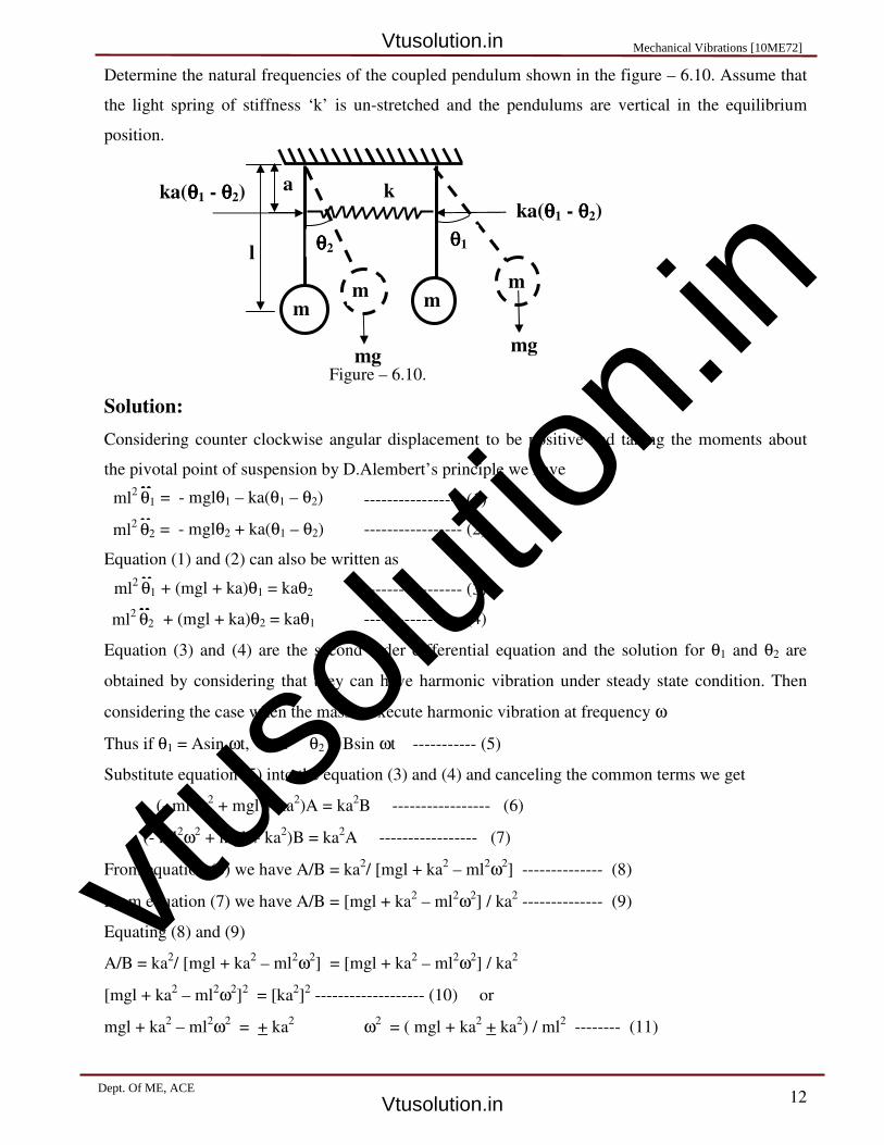
vtuso
lution
.in
12
Determine the natural frequencies of the coupled pendulum shown in the figure – 6.10. Assume that
the light spring of stiffness ‘k’ is un-stretched and the pendulums are vertical in the equilibrium
position.
Figure – 6.10.
Solution:
Considering counter clockwise angular displacement to be positive and taking the moments about
the pivotal point of suspension by D.Alembert’s principle we have
----------------- (1)
----------------- (2)
Equation (1) and (2) can also be written as
----------------- (3)
----------------- (4)
Equation (3) and (4) are the second order differential equation and the solution for θ1 and θ2 are
obtained by considering that they can have harmonic vibration under steady state condition. Then
considering the case when the masses execute harmonic vibration at frequency ω
Thus if θ1 = Asin ωt, and θ2 = Bsin ωt ----------- (5)
Substitute equation (5) into the equation (3) and (4) and canceling the common terms we get
(- ml2ω
2 + mgl + ka
2)A = ka
2B ----------------- (6)
(- ml2ω
2 + mgl + ka
2)B = ka
2A ----------------- (7)
From equation (6) we have A/B = ka2/ [mgl + ka
2 – ml
2ω
2] -------------- (8)
From equation (7) we have A/B = [mgl + ka2 – ml
2ω
2] / ka
2 -------------- (9)
Equating (8) and (9)
A/B = ka2/ [mgl + ka
2 – ml
2ω
2] = [mgl + ka
2 – ml
2ω
2] / ka
2
[mgl + ka2 – ml
2ω
2]
2 = [ka
2]2 ------------------- (10) or
mgl + ka2 – ml
2ω
2 = + ka
2 ω
2 = ( mgl + ka
2 + ka
2) / ml
2 -------- (11)
θ θ θ θ2
m
m m
θθθθ1
k
mg
l
a
mg
ka(θθθθ1 - θθθθ2)
m
ka(θθθθ1 - θθθθ2)
= - mglθ2 + ka(θ1 – θ2) ..
ml2
θ2
+ (mgl + ka)θ1 = kaθ2 ..
ml2
θ1
+ (mgl + ka)θ2 = kaθ1 ..
ml2
θ2
= - mglθ1 – ka(θ1 – θ2) ..
ml2
θ1
Mechanical Vibrations [10ME72]
Dept. Of ME, ACE
Vtusolution.in
Vtusolution.in
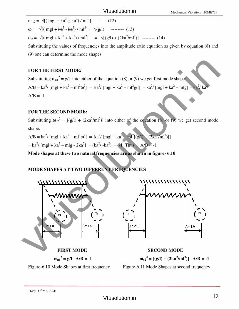
vtuso
lution
.in
ω1,2 = √[( mgl + ka2 + ka
2) / ml
2]
ω1 = √[( mgl + ka2 - ka
2) / ml
2]
ω2 = √[( mgl + ka2 + ka
2) / ml
2] =
Substituting the values of frequencies
(9) one can determine the mode shapes:
FOR THE FIRST MODE:
Substituting ωn12 = g/l into either of the equation (8) or (9) we get first mode shape:
A/B = ka2/ [mgl + ka
2 – ml
2ω
2] = ka
A/B = 1
FOR THE SECOND MODE:
Substituting ωn22 = [(g/l) + (2ka
shape:
A/B = ka2/ [mgl + ka
2 – ml
2ω
2] = ka
= ka2/ [mgl + ka
2 – mlg - 2ka
2] = (ka
Mode shapes at these two natural frequencies are as shown in figure
MODE SHAPES AT TWO DIFFERENT FREQUENCIES
FIRST MODE
ωωωωn12 = g/l A/B = 1
Figure-6.10 Mode Shapes at first frequency
] -------- (12)
= √(g/l) -------- (13)
] = √[(g/l) + (2ka2/ml
2)] -------- (14)
Substituting the values of frequencies into the amplitude ratio equation as given by equation (8) and
(9) one can determine the mode shapes:
= g/l into either of the equation (8) or (9) we get first mode shape:
] = ka2/ [mgl + ka
2 – ml
2g/l] = ka
2/ [mgl + ka
2 –
= [(g/l) + (2ka2/ml
2)] into either of the equation (8) or (9) we get second mode
] = ka2/ [mgl + ka
2 – ml
2[(g/l) + (2ka
2/ml
2)]]
] = (ka2/ -ka
2) = -1 Thus A/B = -1
Mode shapes at these two natural frequencies are as shown in figure- 6.10
MODE SHAPES AT TWO DIFFERENT FREQUENCIES
SECOND MODE
= g/l A/B = 1 ωωωωn22 = [(g/l) + (2ka
2/ml
at first frequency Figure-6.11 Mode Shapes at second frequency
13
into the amplitude ratio equation as given by equation (8) and
= g/l into either of the equation (8) or (9) we get first mode shape:
mlg] = ka2/ ka
2
)] into either of the equation (8) or (9) we get second mode
SECOND MODE
/ml2)] A/B = -1
at second frequency
Mechanical Vibrations [10ME72]
Dept. Of ME, ACE
Vtusolution.in
Vtusolution.in

vtuso
lution
.in
14
m m2
l2 l1
Derive the equation of motion of the system shown in figure 6.12. Assume that the initial tension ‘T’
in the string is too large and remains constants for small amplitudes. Determine the natural
frequencies, the ratio of amplitudes and locate the nodes for each mode of vibrations when m1 = m2
= m and l1= l2 = l3 = l.
Figure 6.12.
At any given instant of time let y1 and y2 be the displacement of the two masses m1 and m2
respectively. The configuration is as shown in the figure 6.13.
(a) (b)
Figure 6.13. Figure 6.14
The forces acting on the two masses are shown in the free body diagram in figure 6.14(a) and (b)
From figure 6.13 we have sinθ1 = (y1/l1) sinθ2 = [(y1 – y2)/l2] and sinθ3 = (y2/l3)
For small angle we have sinθ1 = θ1 = (y1/l1), sinθ2 = θ2 = [(y1 – y2)/l2] and sinθ3 = θ3 = (y2/l3)
and cosθ1 = cosθ2 = cosθ3 = 1.0 Thus the equation of motion for lateral movement of the masses
For the mass m1
or
For the mass m2
or
sin
θθθθ
θθθθ1
θθθθ2
θθθθ3
θθθθ3
3y1
2y2
2
m1
θθθθ1
θθθθ2
T Tcosθθθθ
T
Tcosθθθθ
T(sinθθθθ1+ T
T
Tcosθθθθ Tcosθθθθ
Tsinθθθθ
.. y2
θθθθ2
θθθθ3
m2
y1
..
m1y1 + [(T/l1) + (T/l2)]y1 = (T/l2)y2 ---- (1) ..
.. m1y1 = - (Tsinθ1 + Tsinθ2) = - T (θ1 + θ2)
m1y1 = - T [(y1 /l1) + (y1- y2) /l2] ..
.. m2y2 = (Tsinθ2 – Tsinθ3)
m2y2 = T[(y1- y2) /l2 - (y2 /l3)] ..
y2 + [(T/l2) +(T/l3)]y2 = (T/l2)y1 ----- (2)
Mechanical Vibrations [10ME72]
Dept. Of ME, ACE
Vtusolution.in
Vtusolution.in

vtuso
lution
.in
15
Assuming harmonic motion as y1 =Asinωt and y2 = Bsinωt ------- (3) and substituting this
into equation (1) and (2) we have [-m1ω2 + (T/l1) + (T/l2)] A = (T/l2) B ----- (4)
[-m2ω2 + (T/l2) + (T/l3)] B = (T/l2) A ----- (5)
Thus from equation (4) we have A/B = (T/l2) / [(T/l1) + (T/l2) - m1ω2] ----- (6)
and from equation (5) we have A/B = [(T/l2) + (T/l3) - m2ω2] / (T/l2) ----- (7)
Equating equation (6) and (7) we have A/B=(T/l2)/[(T/l1)+(T/l2)- m1ω2]/[(T/l2)+(T/l3)-m2ω
2]/(T/l2)
Thus we have [(T/l1)+(T/l2)–m1ω2][(T/l2)+(T/l3)-m2ω
2] = (T
2/l2
2) -------------- (8)
Equation (8) is the equation on motion which is also known as frequency equation. Solving this
equation gives the natural frequencies of the system.
Particular Case: When m1 = m2 = m and l1 = l2 = l3 = l then equation (6) can be written as
A/B = (T/l)/[(T/l)+(T/l)-mω2] = (T/l)/[(2T/l)-mω
2] ---------- (9)
and equation (7) can be written as A/B = [(T/l)+(T/l) -mω2]/(T/l) = [(2T/l) - mω
2]/(T/l) ---- (10)
Equating equation (9) and (10) we have [(2T/l - mω2]
2 = (T/l)
2 -------- (11)
Thus 2T/l - mω2 = + (T/l) ------- (12) Therefore we have ω
2 = [(2T+T)]/ml ------ (13)
ωn1 = √[(2T-T]/ml] = √(T/ml) -------- (14) and ωn2 = √[(2T+T]/ml] = √(3T/ml) --------- (15)
Substituting equation (14) and (15) into either of the equation (9) or (10) we have the ratio of
amplitudes for the two natural frequencies. For the first natural frequency ωn1 = √(T/ml) then from
equation (9) we have (A/B)ωn1 = (T/l)/[(2T/l)-mω2] = (T/l)/[(2T/l) – m(T/ml)] = (T/l)/(T/l) = +1
or from equation (10) we have (A/B)ωn1 = [(2T/l) - mω2]/(T/l) = [(2T/l) – m(T/ml)]/(T/l)
Thus (A/B)ωn1 = (T/l)/(T/l) = +1
For the second natural frequency ωn2 = √(3T/ml) then from equation (9) we have
(A/B)ωn2 = (T/l)/[(2T/l)-mω2] = (T/l)/[(2T/l) – m(3T/ml)] = (T/l)/(-T/l) = -1
Thus (A/B)ωn2 = (T/l)/(-T/l) = -1 Then the mode shape will be as shown in figure 6.15(a) and (b)
Figure 6.15(a) Figure 6.15(b)
First Mode ωn1=√(T/ml), (A/B)ωn1 = +1 Second Mode ωn2=√(3T/ml), (A/B)ωn1 = -1
+1 +1 m1 m2 m1
+1
m2 -1
Mechanical Vibrations [10ME72]
Dept. Of ME, ACE
Vtusolution.in
Vtusolution.in

vtuso
lution
.in
16
θθθθ1 J1
θθθθ2 J2
Kt1
Kt2
Torsional Vibratory systems
Derive the equation of motion of a torsional system shown in figure 6.16. Let J1 and J2 be the mass
moment of inertia of the two rotors which are coupled by shafts having torsional stiffness of Kt1 and
Kt2.
Figure 6.16 Two Degree of Freedom Figure 6.17 Free Body Diagram
torsional system
If θ1 and θ2 are the angular displacement of the two rotors at any given instant of time, then the shaft
with the torsional stiffness Kt1 exerts a torque of Kt1θ1 and the shaft with the torsional stiffness Kt2
exerts a torque of Kt2(θ2- θ1) as shown in the free body diagram figure 6.17
Then by Newton second law of motion we have for the mass m1
or
for the mass m2
or
Equation (1) and (2) are the governing Equations of motion of the system.
Equivalent Shaft for a Torsional system
In many engineering applications we find shaft of different diameters as shown in Figure 6.18 are in
use.
Figure-6.18 Stepped shaft
Disc-1
Disc-2
Kt1θθθθ1 Jθθθθ1 ..
Jθθθθ2
..
θθθθ2
θθθθ1
Kt2(θθθθ2 - θθθθ1)
.. J1θ1 = - K1θ1 + K2(θ2 – θ1)
.. J1θ1+( K1+ K2)θ1 = K2θ2 ------ (1)
.. J2θ2 = - K2(θ2 – θ1)
.. J2θ2 + K2θ2 = K2θ1 -------- (2)
d1 d2 d3 d4 J1θθθθ J2 J3 J4
1m2 2 3 4
L1 L2 L3 L4
Ja JB
Mechanical Vibrations[10ME72]
Dept. Of ME, ACE
Vtusolution.in
Vtusolution.in

vtuso
lution
.in
17
For vibration analysis it is required to have an equivalent system. In this section we will study how
to obtain the torsionally equivalent shaft. Let θ be the total angle of twist in the shaft by application
of torque T, and θ1, θ2, θ3 and θ4 be twists in section 1, 2, 3 and 4 respectively. Then we have
θ = θ1 + θ2 + θ3 + θ4
From torsion theory we have,
T = Gθ Where J = pd4/32 Polar moment of inertia of shaft.
J L
Thus θ = θ1 + θ2 + θ3 + θ4 will be
θ = TL1 + TL2 + TL3 + TL4
J1G1 J2G2 J3G3 J4G4
If material of shaft is same, then the above equation can be written as
θ = 32T [ L1 + L2 + L3 + L4 ]
πG [ d14 d2
4 d3
4 d4
4]
If de and Le are equivalent diameter and lengths of the shaft, then:
Le = [ L1 + L2 + L3 + L4 ]
de [ d14 d2
4 d3
4 d4
4]
Le= L1[ de] + L2[ de ] + L3[ de ] + L4[ de ]
[d14] [d2
4] [d3
4] [d4
4]
Equivalent shaft of the system shown in Figure- 6.19
Figure – 6.19 Equivalent shaft of the system shown in figure – 6.18
Definite and Semi-Definite Systems
Definite Systems
A system, which is fixed from one end or both the ends is referred as definite system. A definite
system has nonzero lower natural frequency. A system, which is free from both the ends, is referred
as semi-definite system. For semi-definite systems, the first natural frequency is zero.
Various definite linear and a torsional systems are shown in figure-6.19
de
Le
JA JB
Mechanical Vibrations [10ME72]
Dept. Of ME, ACEDept. Of ME, ACE
Vtusolution.in
Vtusolution.in
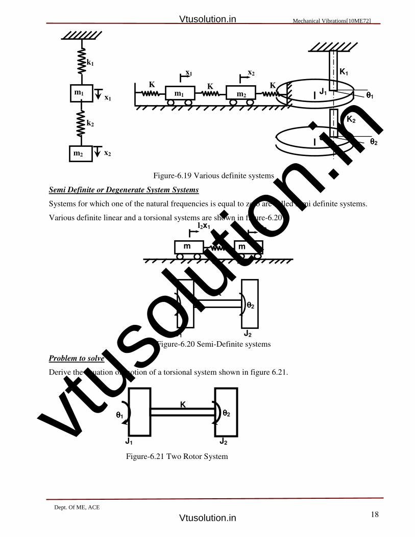
vtuso
lution
.in
18
Figure-6.19 Various definite systems
Semi Definite or Degenerate System Systems
Systems for which one of the natural frequencies is equal to zero are called semi definite systems.
Various definite linear and a torsional systems are shown in figure-6.20
Figure-6.20 Semi-Definite systems
Problem to solve
Derive the equation of motion of a torsional system shown in figure 6.21.
Figure-6.21 Two Rotor System
m1
m2
x1
k2
x2
k1
K1
J1 θθθθ1
J2
K2
θθθθ2
m1 m2 K K K
x1 x2
θθθθ2 K
J2 J1
θθθθ1
m m K
θθθθ2
K
J2 J1
x2 l2x1
Mechanical Vibrations[10ME72]
Dept. Of ME, ACE
Vtusolution.in
Vtusolution.in
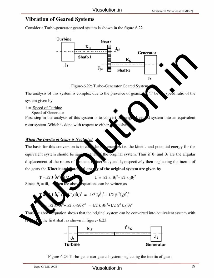
vtuso
lution
.in
19
Generator
Gears
Shaft-1
J1
J2
Jg1
Jg2
Kt1
Kt2
Turbine
Shaft-2
Vibration of Geared Systems
Consider a Turbo-generator geared system is shown in the figure 6.22.
Figure-6.22: Turbo-Generator Geared System.
The analysis of this system is complex due to the presence of gears. Let ‘i’ be the speed ratio of the
system given by
i = Speed of Turbine
Speed of Generator
First step in the analysis of this system is to convert the original geared system into an equivalent
rotor system. Which is done with respect to either of the shafts.
When the Inertia of Gears is Neglected
The basis for this conversion is to consider the energies i.e. the kinetic and potential energy for the
equivalent system should be same as that of the original system. Thus if θ1 and θ2 are the angular
displacement of the rotors of moment of inertia J1 and J2 respectively then neglecting the inertia of
the gears the Kinetic and Potential energy of the original system are given by
Since θ2 = iθ1 Then the above equations can be written as
Thus the above equation shows that the original system can be converted into equivalent system with
respect to the first shaft as shown in figure- 6.23
Figure-6.23 Turbo-generator geared system neglecting the inertia of gears
U = 1/2 kt1θ12+1/2 kt2θ2
2
T =1/2 J1θ12
+ 1/2 J2θ22
. .
T =1/2 J1θ12
+ 1/2 J2(iθ2)2 = 1/2 J1θ1
2 + 1/2 (i
2J2)θ1
2
. . . .
U = 1/2 kt1θ12+1/2 kt2(iθ2)
2 = 1/2 kt1θ1
2+1/2 (i
2 kt2)θ1
2
Generator
J1
kt1
Turbine
i2kt2
J2
Mechanical Vibrations [10ME72]
Dept. Of ME, ACE
Vtusolution.in
Vtusolution.in
vtuso
lution
.in
20
l1
m, J G
K2 K1
Which is obtained by multiplying the inertia and stiffness of the second shaft by i2 and keeping this
part of the system in series with the first part. Thus the stiffness of this equivalent two rotor system is
Thus the frequency of the system is given by
When the Inertia of Gears is Considered
If the inertia of the gears is not negligible then the equivalent system with respect to the first shaft
can be obtained in the same manner and finally we have the three rotor system as shown in figure-
6.24
Figure-6.24 Considering the inertia of gears
CO-ORDINATE COUPLING AND PRINCIPAL COORDINATES.
Consider a two degree of freedom system as shown in the figure- 6.25. The vibration is restricted in
plane of paper.
Figure-6.25. Two degree of freedom system
If m is the mass of the system, J is the Mass Moment of Inertia the system and G is the centre of
gravity. k1 and k2 are the stiffness of the springs which are at a distance ‘l1’ and ‘l2’ from the line
passing through the centre of gravity of the mass.
Then the system has two generalized co-ordinates, x is in Cartesian and θ is in Polar co-ordinate
systems when it is vibrating.
kte = i2 kt1kt2 / (kt1 + i
2 kt2)
ωn = kte(J1 + i2 J2) / i
2 J1J2 rad/sec
J1 J2
Jg1+i2Jg2
Generator
kt1 i2kt2
Turbine
Mechanical Vibrations[10ME72]
Dept. Of ME, ACE
Vtusolution.in
Vtusolution.in
vtuso
lution
.in
21
At any given instant of time for a small disturbance the system occupy the position as shown in
figure-6.26(a).
Figure-6.26 (a) system under vibration (b) displacements at the springs
If ‘x’ is the displacement at the center of gravity of the system. Then the amount of displacements
that take place at the left spring is (x–l1θ)and at the right spring is (x+ l2θ) which is as shown in
figur-6.26(b).
At any given instant of time when the body is displaced through a rectilinear displacement ‘x’ and an
angular displacement ‘θ’ from its equilibrium position. The left spring with the stiffness k1 and the
right spring with the stiffness k2 are compressed through (x–l1θ) and (x+l2θ) from their equilibrium
position, The forces acting on the system is as shown in the free body diagram in figure-6.26. The
differential equation of motion of the system in ‘x’ and ‘θ’ direction are written by considering the
forces and moments in their respective direction.
Thus we have the equation of motion
Rearranging the above two equation we have
Since J = mr2 The above two equation can also be written as
Letting [(k1 + k2)/m = a, (k1l1 - k2l2)/ m = b and (k1l12 + k2l2
2)/ mr
2 = c
Thus substituting these into equation (5) and (6) we have
G
K1 K2
m,J
l1 l2
Static equilibrium
(x – l1θθθθ) (x + l2θθθθ)
θθθθ
x
G
l1 l2
k1(x-l1θθθθ) k2(x + l2θθθθ)
- k (x+l θθθθ)
..
Jθ =+k1(x-l1θ)l1 - k2(x+l2θ)l2 ----- (2)
..
mx + (k1 + k2)x = ( k1l1 - k2l2)θ ----- (3) Jθ + (k1l12 + k2l2
2) θ = (k1l1- k2l2) x ----- (4)
..
θ + [(k1l12
+ k2l22)/ mr
2] θ = [(k1l1- k2l2)/ mr
2] x ----- (6)
..
..
mx = - k1(x - l1θ) - k2(x + l2θ) ----- (1)
..
x + [(k1 + k2)/m]x = [( k1l1 - k2l2)/ m]θ ----- (5)
Mechanical Vibrations [10ME72]
Dept. Of ME, ACE
Vtusolution.in
Vtusolution.in
vtuso
lution
.in
22
The above two differential equation (7) and (8) are coupled with respect to the coordinates in which
‘b’ is called the coupling coefficient or coordinate coupling.
Since if b=0 the two coordinate coupling equations (7) and (8) are independent of each other. The
two equations are then decoupled and each equation may be solved independently of the other. Such
a coordinate are called PRINCIPAL COORDINATE OR NORMAL COORDINATES.
Therefore the two i.e. rectilinear and angular motions can exists independently of each other with
their natural frequency as √a and √c.
Thus for the case of decoupled system when b=0 then (k1l1 – k2l2)/m = 0 or k1l1 – k2l2 = 0 or k1l1 =
k2l2. Then the natural in rectilinear and angular modes are ωnl = √a and ωna = √c
ωnl = √a = √(k1 + k2)/m and ωna = √c = √(k1l12
+ k2l22)/ mr
2
In general for a two degree of freedom under damped free vibration the equation of motion can be
written in the matrix form as
m11 m12 x1 c11 c12 x1 k11 k12 x1 0
+ + =
m21 m22 x2 c21 c22 x2 k21 k22 x2 0
Which reveal the type of coupling present in the system as Dynamic or Mass Coupling exist if the
mass matrix is non diagonal matrix. Where as stiffness or static Coupling exist if the stiffness matrix
is non diagonal. Where as damping Coupling exist if the damping matrix is non diagonal.
The system is dynamically decoupled when the mass matrix exists is a diagonal matrix.
m11 0 x1 c11 c12 x1 k11 k12 x1 0
+ + =
0 m22 x2 c21 c22 x2 k21 k22 x2 0
The system is damped decoupled when the damping matrix exists is a diagonal matrix.
m11 m12 x1 c11 0 x1 k11 k12 x1 0
+ + =
m21 m22 x2 0 c22 x2 k21 k22 x2 0
..
x + ax = bθ ----- (7)
θ + c θ = (b/r2) x ----- (8)
..
..
..
.
.
..
.
.
..
..
.
.
Mechanical Vibrations[10ME72]
Dept. Of ME, ACE
Vtusolution.in
Vtusolution.in

vtuso
lution
.in
23
The system is statically decoupled when the stiffness matrix exists is a diagonal matrix.
m11 m12 x1 c11 c12 x1 k11 0 x1 0
+ + =
m21 m22 x2 c21 c22 x2 0 k22 x2 0
Dynamic or Mass Coupling:
If there is some point ‘C’ in the system along which a force is applied to the system produces pure
translation along the line of action of force as shown in figure-6.27
Figure-6.27 (a) system under vibration (b) displacements at the springs
Then the equation of motion is
Rearranging the above two equation we have
The above equation can be written in matrix form as
When k2l4 – k1l3 = 0 or k2l4 = k1l3 then the system is statically decoupled but dynamically coupled in
which the equation of motion will be which was
Mxc + meθ = -k1(xc-l3θ) - k2(xc+l4θ) ..
..
Jθ + mexc + (k2l4 - k1l3)xc + (k1l32 + k2 l4
2) θ = 0
..
..
Mxc + meθ + (k1+ k2)xc + (k2l4- k2l3)θ = 0 ..
..
Jθ + mexc= -k1(xc-l3θ) - k2(xc+l4θ) ..
..
.. xc
θ
.. (k1+ k2) (k2l4- k1l3)
(k2l4- k1l3) (k1l32+ k2l4
2)
+
xc
θ
0
0
=
M me
me J
(xc-l3θθθθ)(xc+ l4θθθθ)
θθθθ
xc
C
k1(x-l3θθθθ) k2(x+l4θθθθ)
G
l3 l4
Static equilibrium line
G
k1 k2
M,J
l1 l2
C
l3 l4
e e
..
..
.
.
Mechanical Vibrations [10ME72]
Dept. Of ME, ACE
Vtusolution.in
Vtusolution.in

vtuso
lution
.in
24
Static/Stiffness and Dynamic/Mass Coupling: If there is a point ‘C’ in the system along which a
displacement produces pure translation along the line of action of spring force as shown in
figure-6.28
Figure-6.28 (a) system under vibration (b) displacements at the springs
Then the equation of motion is
and
Rearranging the above two equation we have
The above equation can be written in matrix form as
In which both the mass matrix and stiffness matrix are non-diagonal matrix hence the system is both
statically and dynamically coupled.
.. xc
θ
.. (k1+ k2) 0
0 (k1l32+ k2l4
2)
+
xc
θ
0
0
=
M me
me J
xc
(xc+ lθθθθ) θθθθ
C
k1xc k2(xc + lθθθθ)
G
l1 l2
Static equilibrium line
G
k1 k2
M,J
l1 l2
C
l
l
Jθ + ml1xc + k2lxc + k1l2
θ = 0 ..
..
Mxc + ml1θ + (k1+ k2)xc + k2l = 0 ..
..
Mxc + ml1θ = - k1xc - k2(xc+lθ) ..
..
Jθ + m l1xc= -k2(xc+ lθ)l ..
..
+
.. xc
θ
.. (k1+ k2) k2l
k2l k2l2
xc
θ
0
0
=
M ml1
ml1 J
Mechanical Vibrations[10ME72]
Dept. Of ME, ACE
Vtusolution.in
Vtusolution.in

vtuso
lution
.in
25
θ x K1
L1 L2
K2
Problem
Determine the normal mode of vibration of an automobile shown in figure-6.29 simulated by a
simplified two degree of freedom system with the following numerical values m = 1460 kg,
L1 = 1.35m, L2 = 2.65 m, K1 = 4.2x10⁵N/m, K2 = 4.55x10
5 N/m and J=mr
2 where r= 1.22 m
Figure-6.29
Automobile can be modeled as shown in figure -6.30
Figure-6.30 (a) system under vibration (b) displacements at the springs
Let at any given instant of time the translatory displacement be ‘x’ and an angular displacement be
‘θ’ from its equilibrium position of the automobile. Then the left spring with the stiffness k1 and the
right spring with the stiffness k2 are compressed through (x–l1θ) and (x+l2θ) from their equilibrium
position, The forces acting on the system are as shown in the free body diagram in figure-6.30(b).
The differential equation of motion of the automobile in ‘x’ and ‘θ’ direction are written by
considering the forces and moments in their respective direction.
Thus we have the equation of motion
G
K1 K2
m,J
l1 l2
Static equilibrium line
(x – l1θθθθ) (x + l2θθθθ)
θθθθ
x
G
l1 l2
k1(x-l1θθθθ) k2(x + l2θθθθ)
- k (x+l θθθθ)
..
Jθ =+k1(x-l1θ)l1 - k2(x+l2θ)l2 ----- (2)
..
mx = - k1(x - l1θ) - k2(x + l2θ) ----- (1)
Mechanical Vibrations [10ME72]
Dept. Of ME, ACE
Vtusolution.in
Vtusolution.in

vtuso
lution
.in
26
Rearranging the above two equation we have
Equation (3) and (4) are the second order differential equation and the solution for x and θ are
obtained by considering that they can have harmonic vibration under steady state condition. Then
considering the case when the system execute harmonic vibration at frequency ω
Thus if x = Asinωt, and θ = Bsin ωt ---- (5) Substitute equation (5) into the equation (3) and (4) and
canceling the common term sinωt we get
[- mω2 + (k1 + k2)] A = (k1l1 – k2l2) B ------- (6)
[- Jω2 + (k1l1
2 + k2l2
2)] B = (k1l1 – k2l2) A ---- (7)
From equation (6) we have A/B = (k1l1-k2l2)/ [(k1 + k2) – mω2] ---------- (8)
From equation (7) we have A/B = [(k1l12 + k2l2
2) - Jω
2] / (k1l1 – k2l2) ---- (9)
Equating (8) and (9) A/B = (k1l1-k2l2)/ [(k1 + k2) – mω2] = [(k1l1
2 + k2l2
2) - Jω2] / (k1l1 – k2l2)
[(k1+k2)–mω2][(k1l1
2+k2l2
2)-Jω
2]=(k1l1-k2l2)
2 Further Simplification will give
mJω4–[J(k1+k2) + m(k1l1
2+k2l2
2)]ω
2 + k1k2(l1+l2)
2 = 0 --------- (10)
Substituting the value of m, J, k1, k2, l1, l2 into the above equation (10) we have
3.173x10⁶ω
4– 4.831x10
9ω
2+1.72x10
12=0 --- (11) or ω
4– 1.523x10³ω
2+5.429x10
5=0 ---- (12)
Letting ω2 =λ we have λ
2– 1.523x10
3λ+5.429x10
5 = 0 ---- (13)
Equation (13) is quadratic equation in λ. Thus solving equation (13) we get two roots which are
λ1= 569.59, λ2= 953.13 Since ω2
=λ we have ω = √λ. Thus ω1=23.86 rad/sec and ω2=30.87 rad/sec
Thus fn1 = 3.797 Hz and fn2 = 4.911 Hz
Un-damped Dynamic Vibration Absorber
Consider a two degree of freedom system with a forcing function F1 = Fosinωt as shown in
figure-6.31(a).
(a) (b)
Figure- 6.31(a) Two degree of freedom system with forcing function F1 on mass 1
..
mx + (k1 + k2)x = ( k1l1 - k2l2)θ ----- (3)
Jθ + (k1l12 + k2l2
2) θ = (k1l1- k2l2) x ----- (4)
..
m1
m2
k2
k1
x1
x2
F1
m1
m2
k2 (x2 –
x )
k1x1
F1 = Fosinωωωωt
Mechanical Vibrations [10ME72]
Dept. Of ME, ACE
Vtusolution.in
Vtusolution.in
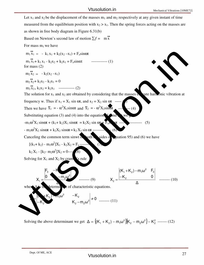
vtuso
lution
.in
27
Let x1 and x2 be the displacement of the masses m1 and m2 respectively at any given instant of time
measured from the equilibrium position with x2 > x1. Then the spring forces acting on the masses are
as shown in free body diagram in Figure 6.31(b)
Based on Newton’s second law of motion ∑ƒ =
For mass m1 we have
for mass (2)
The solution for x1 and x2 are obtained by considering that the masses execute harmonic vibration at
frequency w. Thus if x1 = X1 sin ωt, and x2 = X2 sin ωt ----- (3)
Then we have and --------- (4)
Substituting equation (3) and (4) into the equation (1) and (2) we get
-m1ω2X1 sinωt + (k1+ k2)X1 sinωt = k2X2 sin ωt + Fosinωt ----------------- (5)
- m2ω2X2 sinωt + k2X2 sinωt = k2 X1 sin ωt -------------- (6)
Canceling the common term sinwt on both the sides of equation 95) and (6) we have
[(k1+ k2) - m1ω2]X1 - k2X2 = Fo ----------- (7)
k2 X1 - [k2- m2ω2]X2 = 0----- (8)
Solving for X1 and X2 by cramer’s rule
-------- (9) -------- (10)
where ∆ is the determinant of characteristic equations.
-------- (11)
Solving the above determinant we get ------- (12)
..
x1 = - ω2X1sinωt
..
x2 = - ω2X2sinωt
.. m x
.. m2 x2 + k2x2 - k2x1 = 0
.. m2 x2 + k2x2 = k2x1 ------------ (2)
= ..
m2 x2 - k2(x2 –x1)
= ..
m1 x1 - k1 x1 + k2(x2 –x1) + Fosinωt
.. m1 x1 + k1 x1 - k2x2 + k2x1 = Fosinωt ------------ (1)
{ }{ } 2
2
2
22
2
121KωmKωm)K(K∆ −−−+=
∆
ωmK
K
0
F
X
2
22
20
1
−
−
=∆
0
F
K
ωm)K(K
X
0
2
2
121
2
−
−+
=
0ωmK
K
K
ωm)K(K∆
2
22
2
2
2
121 ≠−
−
−
−+=
Mechanical Vibrations [10ME72]
Dept. Of ME, ACE
Vtusolution.in
Vtusolution.in

vtuso
lution
.in
28
If the two vibratory masses are considered separately as shown in Figure- 6.32, the mass 1 is a main
system and mass 2 is an secondary system. This system can be used as Dynamic vibration absorber
or Tuned damper by using the amplitude Equations (9) and (10).
Figure- 6.32
If the system has to be used as a Dynamic vibration absorber, then the amplitude of vibration of
mass m1 should be equal to zero, i.e X1=0.
-------- (13) Then we have
Fo(k2 – m2ωωωω2) = 0 since Fo cannot be equal to zero we have k2 – m2ωωωω
2 = 0
ωωωω2 = k2 /m2 or ωωωω
= √ k2 /m2 rad/sec -------- (14)
The above Eqn. is the natural frequency of secondary or absorber system.
0∆
ωmK
K
0
F
X
2
22
20
1=
−
−
=0
ωmK
K
0
F
2
22
20=
−
−
m1
m2
k2
k1
x1
x2
F1 Main System
Secondary System
Dept. Of ME, ACE
Mechanical vibraMechanical Vibrations [10ME72]Vtusolution.in
Vtusolution.in

vtuso
lution
.inMechanical Vibrations (ME 65)
CHAPTER-8
MULTI DEGREE OF FREEDOM SYSTEMS
Topics covered:
Influence co-efficents
Approximate methods
(i) Dunkerley’s method
(ii) Rayleigh’s method
Influence co-efficients
Numerical methods
(i) Matrix iteration method
(ii) Stodola’s method
(iii) Holzar’s method
1. Influence co-efficents
It is the influence of unit displacement at one point on the forces at various points of a
multi-DOF system.
OR
It is the influence of unit Force at one point on the displacements at various points of
a multi-DOF system.
The equations of motion of a multi-degree freedom system can be written in terms of
influence co-efficients. A set of influence co-efficents can be associated with each of
matrices involved in the equations of motion.
[ ]{ } [ ]{ } [ ]0xKxM =+&&
For a simple linear spring the force necessary to cause unit elongation is referred as
stiffness of spring. For a multi-DOF system one can express the relationship between
displacement at a point and forces acting at various other points of the system by
using influence co-efficents referred as stiffness influence coefficents
The equations of motion of a multi-degree freedom system can be written in terms of
inverse of stiffness matrix referred as flexibility influence co-efficients.
Matrix of flexibility influence co-efficients = [ ] 1−K
The elements corresponds to inverse mass matrix are referred as flexibility
mass/inertia co-efficients.
Matrix of flexibility mass/inertia co-efficients =[ ] 1−M
The flexibility influence co-efficients are popular as these coefficents give elements
of inverse of stiffness matrix. The flexibility mass/inertia co-efficients give elements
of inverse of mass matrix
UNIT - 7
NUMERICAL METHODS FOR MULTI DEGREE FREEDOM OF SYSTEMS
Mechanical Vibrations [10ME72]
1Dept. Of ME, ACE
Vtusolution.in
Vtusolution.in

vtuso
lution
.inVTU e-learning Course ME65 Mechanical Vibrations
Prof. S. K. Kudari, Principal APS College of Engineering, Bengaluru-28.
2
Stiffness influence co-efficents.
For a multi-DOF system one can express the relationship between displacement at a
point and forces acting at various other points of the system by using influence co-
efficents referred as stiffness influence coefficents.
{ } [ ]{ }xKF =
[ ]
=
333231
322221
131211
kkk
kkk
kkk
K
wher, k11, ……..k33 are referred as stiffness influence coefficients
k11-stiffness influence coefficient at point 1 due to a unit deflection at point 1
k21- stiffness influence coefficient at point 2 due to a unit deflection at point 1
k31- stiffness influence coefficient at point 3 due to a unit deflection at point 1
Example-1.
Obtain the stiffness coefficients of the system shown in Fig.1.
I-step:
Apply 1 unit deflection at point 1 as shown in Fig.1(a) and write the force equilibrium
equations. We get,
2111KKk +=
221Kk −=
0k31
=
m1
K1
m2
K2
x1=1 Unit
x2=0
m3
K3
x3=0
k11
k21
k31
x2=1 Unit
m1
K1
m2
K2
x1=0
m3
K3
x3=0
K12
k22
k32
m1
K1
m2
K2
x1=0
x2=0
m3
K3
x3=1 Unit
k13
k23
k33
(a) (b) (c)
Fig.1 Stiffness influence coefficients of the system
Mechanical Vibrations [10ME72]
Dept. Of ME, ACE 2
Vtusolution.in
Vtusolution.in

vtuso
lution
.inVTU e-learning Course ME65 Mechanical Vibrations
Prof. S. K. Kudari, Principal APS College of Engineering, Bengaluru-28.
3
II-step:
Apply 1 unit deflection at point 2 as shown in Fig.1(b) and write the force equilibrium
equations. We get,
212-Kk =
3222KKk +=
331-Kk =
III-step:
Apply 1 unit deflection at point 3 as shown in Fig.1(c) and write the force equilibrium
equations. We get,
0k13
=
323-Kk =
333Kk =
[ ]
=
333231
322221
131211
kkk
kkk
kkk
K
[ ]( )
( )
+
+
=
33
3322
221
KK-0
K-KKK-
0K-KK
K
From stiffness coefficients K matrix can be obtained without writing Eqns. of motion.
Flexibility influence co-efficents.
{ } [ ]{ }xKF =
{ } [ ] { }FKx1−
=
{ } [ ]{ }Fαx =
where, [ ]α - Matrix of Flexibility influence co-efficents given by
[ ]
=
333231
322221
131211
ααα
ααα
ααα
α
wher, α11, ……..α33 are referred as stiffness influence coefficients
α11-flexibility influence coefficient at point 1 due to a unit force at point 1
α21- flexibility influence coefficient at point 2 due to a unit force at point 1
α31- flexibility influence coefficient at point 3 due to a unit force at point 1
Example-2.
Obtain the flexibility coefficients of the system shown in Fig.2.
Mechanical Vibrations [10ME72]
3Dept. Of ME, ACE
Vtusolution.in
Vtusolution.in

vtuso
lution
.inVTU e-learning Course ME65 Mechanical Vibrations
Prof. S. K. Kudari, Principal APS College of Engineering, Bengaluru-28.
4
I-step:
Apply 1 unit Force at point 1 as shown in Fig.2(a) and write the force equilibrium
equations. We get,
1
312111K
1ααα ===
II-step:
Apply 1 unit Force at point 2 as shown in Fig.2(b) and write the force equilibrium
equations. We get,
21
3222K
1
K
1αα +==
III-step:
Apply 1 unit Force at point 3 as shown in Fig.2(c) and write the force equilibrium
equations. We get,
21
23K
1
K
1α +=
321
33K
1
K
1
K
1α ++=
Therefore,
1
1331122111K
1ααααα ======
21
233222K
1
K
1ααα +===
321
33K
1
K
1
K
1α ++=
(b) (c)
Fig.2 Flexibility influence coefficients of the system
x2=α22
m1
K1
m2
K2
x1=α12
m3
K3
x3=α32
F1=0
F2=1
F3=0
m1
K1
m2
K2
x1=α13
x2=α23
m3
K3
x3=α33
F1=0
F2=1
F3=0
(a)
m1
K1
m2
K2
m3
K3
x3=α31
F1=0
F2=1
F3=0
x1=α11
x2=α21
Mechanical Vibrations [10ME72]
4Dept. Of ME, ACE
Vtusolution.in
Vtusolution.in

vtuso
lution
.inVTU e-learning Course ME65 Mechanical Vibrations
Prof. S. K. Kudari, Principal APS College of Engineering, Bengaluru-28.
5
For simplification, let us consider : KKKK321
===
K
1
K
1ααααα
1
1331122111=======
K
2
K
1
K
1ααα
233222=+===
K
3
K
1
K
1
K
1α
33=++=
[ ]
=
333231
322221
131211
ααα
ααα
ααα
α
[ ]
=
321
221
111
K
1α
[ ] [ ] 1Kα
−=
In Vibration analysis if there is need of [ ] 1K
−one can use flexibility co-efficent matrix.
Example-3
Obtain of the Flexibility influence co-efficents of the pendulum system shown in the
Fig.3.
I-step:
Apply 1 unit Force at point 1 as shown in Fig.4 and write the force equilibrium
equations. We get,
m
m
l
l
m
l
Fig.3 Pendulum system
m
m
l
l
m
l
F=1
T θ
α11
Fig.4 Flexibility influence
co-efficents
Mechanical Vibrations 10ME72]
5Dept. Of ME, ACE
Vtusolution.in
Vtusolution.in

vtuso
lution
.inVTU e-learning Course ME65 Mechanical Vibrations
Prof. S. K. Kudari, Principal APS College of Engineering, Bengaluru-28.
6
lθ sin T =
3mgm)mg(mθ cos T =++=
3mg
1θ tan =
θ sinθ tan small, is θ =
l
αθ sin
11=
θ sin lα11
=
3mg
lα
11=
Similarly apply 1 unit force at point 2 and next at point 3 to obtain,
5mg
lα
22=
the influence coefficients are:
5mg
lααααα
1331122111======
6mg
11lααα
233222===
6mg
11lα
33=
Approximate methods
In many engineering problems it is required to quickly estimate the first
(fundamental) natural frequency. Approximate methods like Dunkerley’s method,
Rayleigh’s method are used in such cases.
(i) Dunkerley’s method
Dunkerley’s formula can be determined by frequency equation,
[ ] [ ] [ ]0KMω2 =+−
[ ] [ ] [ ]0MωK2 =+−
[ ] [ ] [ ] [ ]0MKIω
1 1
2=+−
−
[ ] [ ][ ] [ ]0MαIω
1
2=+−
For n DOF systems,
Mechanical Vibrations [10ME72]
6Dept. Of ME, ACE
Vtusolution.in
Vtusolution.in

vtuso
lution
.inVTU e-learning Course ME65 Mechanical Vibrations
Prof. S. K. Kudari, Principal APS College of Engineering, Bengaluru-28.
7
[ ]0
m.00
.
0.m0
0.0m
α.αα
.
α.αα
α.αα
1.00
.
0.10
0.01
ω
1
n
2
1
nnn2n1
2n2221
1n1211
2=
+
−
[ ]0
mαω
1.mαmα
.
mα.mαω
10
mα.mαmαω
1
nnn22n21n1
n2n2222
n1n2121112
=
+−
+−
+−
...
Solve the determinant
( )
( ) [ ]0...mα...mmααmmαα
ω
1mα...mαmα
ω
1
nnn313311212211
1n
2nnn222111
n
2
=++++
+++−
−
(1)
It is the polynomial equation of nth degree in (1/ω2). Let the roots of above Eqn. are:
2
n
2
2
2
1ω
1...... ,
ω
1 ,
ω
1
0...ω
1
ω
1......
ω
1
ω
1
ω
1
ω
1
ω
1...... ,
ω
1
ω
1 ,
ω
1
ω
1
1n
22
n
2
2
2
1
n
2
2
n
22
2
22
1
2
=−
+++−
=
−
−
−
− (2)
Comparing Eqn.(1) and Eqn. (2), we get,
=
+++
2
n
2
2
2
1ω
1......
ω
1
ω
1( )
nnn222111mα...mαmα +++
In mechanical systems higher natural frequencies are much larger than the
fundamental (first) natural frequencies. Approximately, the first natural frequency is:
≅
2
1ω
1( )
nnn222111mα...mαmα +++
The above formula is referred as Dunkerley’s formula, which can be used to estimate
first natural frequency of a system approximately.
The natural frequency of the system considering only mass m1 is:
1
1
111
1nm
K
mα
1ω ==
The Dunkerley’s formula can be written as:
2
nn
2
2n
2
1n
2
1ω
1......
ω
1
ω
1
ω
1+++≅ (3)
Mechanical Vibrations [10ME72]
7Dept. Of ME, ACE
Vtusolution.in
Vtusolution.in

vtuso
lution
.inVTU e-learning Course ME65 Mechanical Vibrations
Prof. S. K. Kudari, Principal APS College of Engineering, Bengaluru-28.
8
where, ..... ,ω ,ω2n1n
are natural frequency of single degree of freedom system
considering each mass separately.
The above formula given by Eqn. (3) can be used for any mechanical/structural
system to obtain first natural frequency
Examples: 1
Obtain the approximate fundamental natural frequency of the system shown in Fig.5
using Dunkerley’s method.
Dunkerley’s formula is:
≅
2
1ω
1( )
nnn222111mα...mαmα +++ OR
2
nn
2
2n
2
1n
2
1ω
1......
ω
1
ω
1
ω
1+++≅
Any one of the above formula can be used to find fundamental natural frequency
approximately.
Find influence flexibility coefficients.
K
1ααααα
1331122111=====
K
2ααα
233222===
K
3α
33=
Substitute all influence coefficients in the Dunkerley’s formula.
≅
2
1ω
1( )
nnn222111mα...mαmα +++
m
K
m
K
x1
x2
m
K
x3
Fig.5 Linear vibratory system
Mechanical Vibrations [10ME72]
8Dept. Of ME, ACE
Vtusolution.in
Vtusolution.in

vtuso
lution
.inVTU e-learning Course ME65 Mechanical Vibrations
Prof. S. K. Kudari, Principal APS College of Engineering, Bengaluru-28.
9
≅
2
1ω
1
K
6m
K
3m
K
2m
K
m=
++
K/m0.40ω1=
rad/s
Examples: 2
Find the lowest natural frequency of the system shown in Figure by Dunkerley’s
method. Take m1=100 kg, m2=50 kg
VTU Exam July/Aug 2006 for 20 Marks
Obtain the influence co-efficents:
EI
1.944x10α
-3
11=
EI
9x10α
-3
22=
≅
2
nω
1( )
222111mαmα +
rad/s 1.245ωn
=
(ii) Rayleigh’s method
It is an approximate method of finding fundamental natural frequency of a system
using energy principle. This principle is largely used for structural applications.
Principle of Rayleigh’s method
Consider a rotor system as shown in Fig.7. Let, m1, m2 and m3 are masses of rotors on
shaft supported by two bearings at A and B and y1, y2 and y3 are static deflection of
shaft at points 1, 2 and 3.
1 2
180 120
m1 m2
Fig.6 A cantilever rotor system.
Mechanical Vibrations [10ME72]
9Dept. Of ME, ACE
Vtusolution.in
Vtusolution.in

vtuso
lution
.inVTU e-learning Course ME65 Mechanical Vibrations
Prof. S. K. Kudari, Principal APS College of Engineering, Bengaluru-28.
10
For the given system maximum potential energy and kinetic energies are:
∑=
=n
1i
iimaxgym
2
1V (4)
∑=
=n
1i
2
iimaxym
2
1T &
where, mi- masses of the system, yi –displacements at mass points.
Considering the system vibrates with SHM,
i
2
iyωy =&
From above equations
∑=
=n
1i
2
ii
2
maxym
2
ωT (5)
According to Rayleigh’s method,
maxmaxTV = (6)
substitute Eqn. (4) and (5) in (6)
∑
∑
=
==n
1i
2
ii
n
1i
ii
2
ym
gym
ω (7)
The deflections at point 1, 2 and 3 can be found by.
gmαgmαgmαy3132121111
++=
gmαgmαgmαy3232221212
++=
gmαgmαgmαy3332321313
++=
Eqn.(7) is the Rayleigh’s formula, which is used to estimate frequency of transverse
vibrations of a vibratory systems.
1 2 3
m1 m2 m3
A B
y1 y2
y3
Fig.7 A rotor system.
Mechanical Vibrations [10ME72]
10Dept. Of ME, ACE
Vtusolution.in
Vtusolution.in
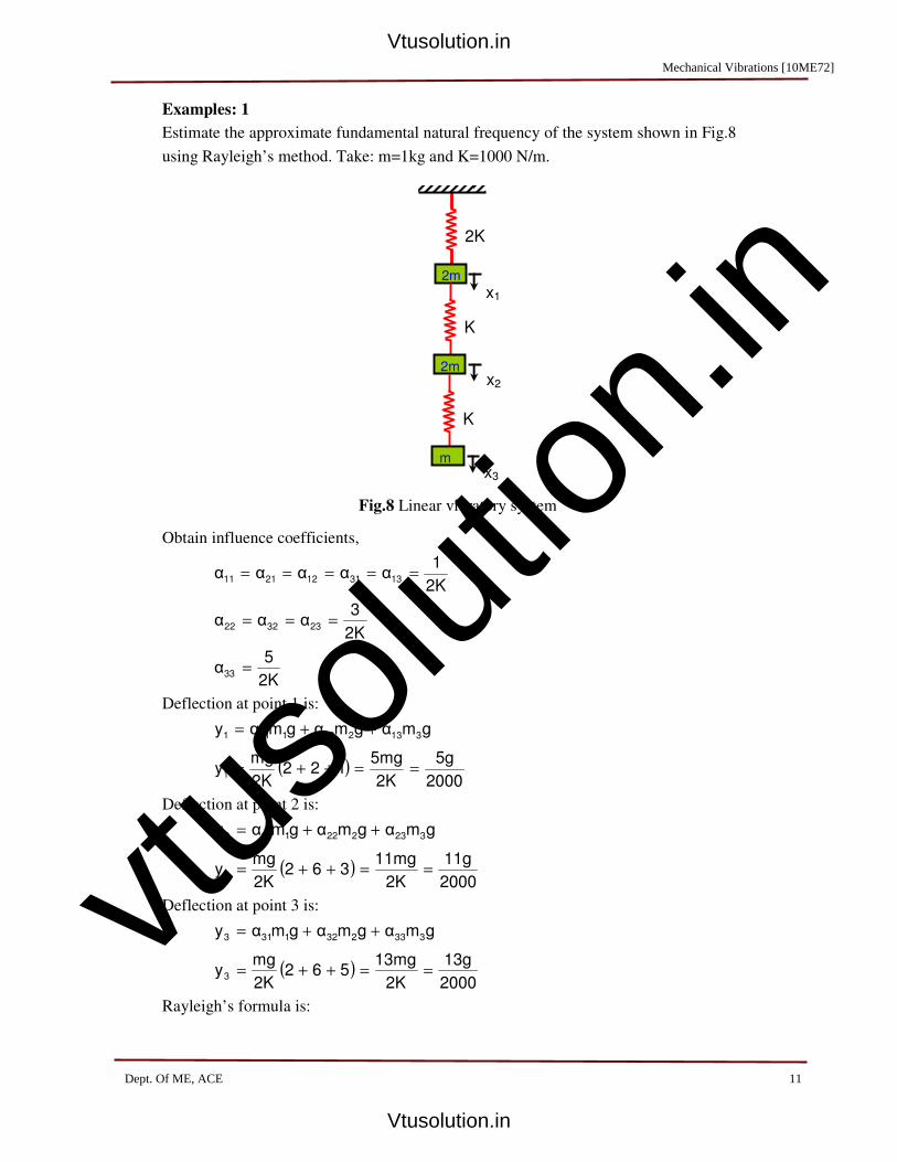
vtuso
lution
.inVTU e-learning Course ME65 Mechanical Vibrations
Prof. S. K. Kudari, Principal APS College of Engineering, Bengaluru-28.
11
Examples: 1
Estimate the approximate fundamental natural frequency of the system shown in Fig.8
using Rayleigh’s method. Take: m=1kg and K=1000 N/m.
Obtain influence coefficients,
2K
1ααααα
1331122111=====
2K
3ααα
233222===
2K
5α
33=
Deflection at point 1 is:
gmαgmαgmαy3132121111
++=
( )2000
5g
2K
5mg122
2K
mgy
1==++=
Deflection at point 2 is:
gmαgmαgmαy3232221212
++=
( )2000
11g
2K
11mg362
2K
mgy
2==++=
Deflection at point 3 is:
gmαgmαgmαy3332321313
++=
( )2000
13g
2K
13mg562
2K
mgy
3==++=
Rayleigh’s formula is:
2m
2K
2m
K
x1
x2
m
K
x3
Fig.8 Linear vibratory system
Mechanical Vibrations [10ME72]
11Dept. Of ME, ACE
Vtusolution.in
Vtusolution.in

vtuso
lution
.inVTU e-learning Course ME65 Mechanical Vibrations
Prof. S. K. Kudari, Principal APS College of Engineering, Bengaluru-28.
12
∑
∑
=
==n
1i
2
ii
n
1i
ii
2
ym
gym
ω
2
222
2
2
g2000
132
2000
112
2000
52
g2000
132x
2000
112x
2000
52x
ω
+
+
++
=
rad/s 12.41ω =
Examples: 2
Find the lowest natural frequency of transverse vibrations of the system shown in
Fig.9 by Rayleigh’s method.
E=196 GPa, I=10-6 m4, m1=40 kg, m2=20 kg
VTU Exam July/Aug 2005 for 20 Marks
Step-1:
Find deflections at point of loading from strength of materials principle.
For a simply supported beam shown in Fig.10, the deflection of beam at distance x
from left is given by:
( ) b)(l xfor bxl6EIl
Wbxy
222 −≤−−=
For the given problem deflection at loads can be obtained by superposition of
deflections due to each load acting separately.
1 2
m1 m2
B
160 80 180
A
Fig.9 A rotor system.
b x
l
W
Fig.10 A simply supported beam
Mechanical Vibrations [10ME72]
12Dept. Of ME, ACE
Vtusolution.in
Vtusolution.in

vtuso
lution
.inVTU e-learning Course ME65 Mechanical Vibrations
Prof. S. K. Kudari, Principal APS College of Engineering, Bengaluru-28.
13
Deflections due to 20 kg mass
( ) ( ) EI
0.2650.180.160.42
6EI0.42
x0.18x0.169.81x20y
222'
1=−−=
( ) ( ) EI
0.290.180.240.42
6EIx0.42
x0.18x0.249.81x20y
222'
2=−−=
Deflections due to 40 kg mass
( ) ( ) EI
0.5380.160.260.42
6EIx0.42
x0.16x0.269.81x40y
222''
1=−−=
( ) ( ) EI
0.530.160.180.42
6EIx0.42
x0.16x0.189.81x40y
222''
2=−−=
The deflection at point 1 is:
EI
0.803yyy
''
1
'
11=+=
The deflection at point 2 is:
EI
0.82yyy
''
2
'
22=+=
∑
∑
=
==n
1i
2
ii
n
1i
ii
2
ym
gym
ω
( )( ) ( )22
2
20x0.8240x0.803
20x0.8240x0.8039.81ω
+
+=
rad/s 1541.9ωn
=
Mechanical Vibrations [10ME72]
13Dept. Of ME,ACE
Vtusolution.in
Vtusolution.in

vtuso
lution
.inVTU e-learning Course ME65 Mechanical Vibrations
Prof. S. K. Kudari, Principal APS College of Engineering, Bengaluru-28.
14
Numerical methods
(i) Matrix iteration method
Using this method one can obtain natural frequencies and modal vectors of a vibratory
system having multi-degree freedom.
It is required to have ω1< ω2<……….< ωn
Eqns. of motion of a vibratory system (having n DOF) in matrix form can be written
as:
[ ]{ } [ ]{ } [ ]0xKxM =+&&
where,
{ } { } ( )φωtsinAx += (8)
substitute Eqn.(8) in (9)
[ ]{ } [ ]{ } [ ]0AKAMω2 =+− (9)
For principal modes of oscillations, for rth
mode,
[ ]{ } [ ]{ } [ ]0AKAMωrr
2
r=+−
[ ] [ ]{ } { }r2
r
rA
ωAMK
11=
−
[ ]{ } { }r2
r
rA
ωAD
1= (10)
where, [ ]D is referred as Dynamic matrix.
Eqn.(10) converges to first natural frequency and first modal vector.
The Equation,
[ ] [ ]{ } { }r
2
rrAωAKM =
−1
[ ]{ } { }r
2
rr1AωAD = (11)
where, [ ]1
D is referred as inverse dynamic matrix.
Eqn.(11) converges to last natural frequency and last modal vector.
In above Eqns (10) and (11) by assuming trial modal vector and iterating till the Eqn
is satisfied, one can estimate natural frequency of a system.
Examples: 1
Find first natural frequency and modal vector of the system shown in the Fig.10 using
matrix iteration method. Use flexibility influence co-efficients.
Find influence coefficients.
2K
1ααααα
1331122111=====
2K
3ααα
233222===
Mechanical Vibrations [10ME72]
14Dept. Of ME, ACE
Vtusolution.in
Vtusolution.in

vtuso
lution
.inVTU e-learning Course ME65 Mechanical Vibrations
Prof. S. K. Kudari, Principal APS College of Engineering, Bengaluru-28.
15
2K
5α
33=
[ ]
=
333231
322221
131211
ααα
ααα
ααα
α
[ ] [ ]
==−
531
331
111
2K
1Kα
1
First natural frequency and modal vector
[ ] [ ]{ } { }r2
r
rA
ωAMK
11=
−
[ ]{ } { }r2
r
rA
ωAD
1=
Obtain Dynamic matrix [ ] [ ] [ ]MKD1−
=
[ ]
=
=
562
362
122
2K
m
100
020
002
531
331
111
2K
mD
Use basic Eqn to obtain first frequency
[ ]{ } { }12
r
1A
ωAD
1=
Assume trial vector and substitute in the above Eqn.
Assumed vector is: { }
=
1
1
1
u1
First Iteration
[ ]{ } =1
uD
1
1
1
562
362
122
2K
m
=
2.6
2.2
1
2K
5m
As the new vector is not matching with the assumed one, iterate again using the new
vector as assumed vector in next iteration.
Mechanical Vibrations [10ME72]
15Dept. Of ME, ACE
Vtusolution.in
Vtusolution.in

vtuso
lution
.inVTU e-learning Course ME65 Mechanical Vibrations
Prof. S. K. Kudari, Principal APS College of Engineering, Bengaluru-28.
16
Second Iteration
[ ]{ } =2
uD
2.6
2.2
1
562
362
122
2K
m
=
3.13
2.55
1
K
4.5m
Third Iteration
[ ]{ } =3
uD
3.133
2.555
1
562
362
122
2K
m
=
3.22
2.61
1
K
5.12m
Fourth Iteration
[ ]{ } =4
uD
3.22
2.61
1
562
362
122
2K
m
=
3.23
2.61
1
K
5.22m
As the vectors are matching stop iterating. The new vector is the modal vector.
To obtain the natural frequency,
[ ]
3.22
2.61
1
D
=
3.23
2.61
1
K
5.22m
Compare above Eqn with with basic Eqn.
[ ]{ } { }12
1
1A
ωAD
1=
K
5.22m
ω
1
2
1
=
m
K
5.22
1ω2
1=
m
K0.437ω
1= Rad/s
Modal vector is:
{ }
=
3.23
2.61
1
A1
Mechanical Vibrations [10ME72]
16Dept. Of ME, ACE
Vtusolution.in
Vtusolution.in

vtuso
lution
.inVTU e-learning Course ME65 Mechanical Vibrations
Prof. S. K. Kudari, Principal APS College of Engineering, Bengaluru-28.
17
Method of obtaining natural frequencies in between first and last one
(Sweeping Technique)
For understanding it is required to to clearly understand Orthogonality principle of
modal vectors.
Orthogonality principle of modal vectors
Consider two vectors shown in Fig.11. Vectors { } { }b and a are orthogonal to each
other if and only if
{ } { } 0baT
=
{ } 0b
baa
2
1
21=
{ } 0b
b
10
01aa
2
1
21=
{ } [ ]{ } 0bIaT
= (12)
where, [ ]I is Identity matrix.
From Eqn.(12), Vectors { } { }b and a are orthogonal to each other with respect to
identity matrix.
Application of orthogonality principle in vibration analysis
Eqns. of motion of a vibratory system (having n DOF) in matrix form can be written
as:
[ ]{ } [ ]{ } [ ]0xKxM =+&&
{ } { } ( )φωtsinAx +=
[ ]{ } [ ]{ } [ ]0AKAMω2 =+− 11
x1
x2
{ }
=2
1
b
bb
{ }
=2
1
a
aa
Fig.11 Vector representation graphically
Mechanical Vibrations [10ME72]
17Dept.Of ME, ACE
Vtusolution.in
Vtusolution.in

vtuso
lution
.inVTU e-learning Course ME65 Mechanical Vibrations
Prof. S. K. Kudari, Principal APS College of Engineering, Bengaluru-28.
18
[ ]{ } [ ]{ }11 AKAMω2 =
If system has two frequencies ω1 and ω2
[ ]{ } [ ]{ }11 AKAMω2
1= (13)
[ ]{ } [ ]{ }22 AKAMω2
2= (14)
Multiply Eqn.(13) by { }T
2A and Eqn.(14) by { }T
1A
{ } [ ]{ } { } [ ]{ }1
T
21
T
2
2
1AKAAMAω = (15)
{ } [ ]{ } { } [ ]{ }2
T
12
T
1
2
1AKAAMAω = (16)
Eqn.(15)-(16)
{ } [ ]{ } 0AMA2
T
1=
Above equation is a condition for mass orthogonality.
{ } [ ]{ } 0AKA2
T
1=
Above equation is a condition for stiffness orthogonality.
By knowing the first modal vector one can easily obtain the second modal vector
based on either mass or stiffness orthogonality. This principle is used in the matrix
iteration method to obtain the second modal vector and second natural frequency.
This technique is referred as Sweeping technique
Sweeping technique
After obtaining { }11
ω and A to obtain { }22
ω and A choose a trial vector { }1
V
orthogonal to { }1
A ,which gives constraint Eqn.:
{ } [ ]{ } 0AMV1
T
1=
{ } 0
A
A
A
m00
0m0
00m
VVV
3
2
1
3
2
1
321=
( ) ( ) ( ){ } 0AmVAmVAmV333222111
=++
( ) ( ) ( ){ } 0VAmVAmVAm333222111
=++
321βVαVV +=
where α and β are constants
−=
11
22
Am
Amα
−=
11
33
Am
Amβ
Therefore the trial vector is:
Mechanical Vibrations [10ME72]
18Dept. Of ME, ACE
Vtusolution.in
Vtusolution.in

vtuso
lution
.inVTU e-learning Course ME65 Mechanical Vibrations
Prof. S. K. Kudari, Principal APS College of Engineering, Bengaluru-28.
19
( )
+
=
3
2
32
3
2
1
V
V
βVαV
V
V
V
=
3
2
1
V
V
V
100
010
βα0
[ ]{ }1VS=
where [ ]S= is referred as Sweeping matrix and { }1V is the trial vector.
New dynamics matrix is:
[ ] [ ][ ]SDDs
+
[ ]{ } { }22
2
1sA
ωVD
1=
The above Eqn. Converges to second natural frequency and second modal vector.
This method of obtaining frequency and modal vectors between first and the last one
is referred as sweeping technique.
Examples: 2
For the Example problem 1, Find second natural frequency and modal vector of the
system shown in the Fig.10 using matrix iteration method and Sweeping technique.
Use flexibility influence co-efficients.
For this example already the first frequency and modal vectors are obtained by matrix
iteration method in Example 1. In this stage only how to obtain second frequency is
demonstrated.
First Modal vector obtained in Example 1 is:
{ }
=
=
3.23
2.61
1
A
A
A
A
3
2
1
1
[ ]
=
100
020
002
M is the mass matrix
Find sweeping matrix
[ ]
=
100
010
βα0
S
2.612(1)
2(2.61)
Am
Amα
11
22 −=
−=
−=
Mechanical Vibrations[10ME72]
19Dept. Of ME, ACE
Vtusolution.in
Vtusolution.in

vtuso
lution
.inVTU e-learning Course ME65 Mechanical Vibrations
Prof. S. K. Kudari, Principal APS College of Engineering, Bengaluru-28.
20
1.6152(1)
1(3.23)
Am
Amβ
11
33 −=
−=
−=
Sweeping matrix is:
[ ]
=
100
010
1.615-2.61-0
S
New Dynamics matrix is:
[ ] [ ][ ]SDDs
+
[ ]
−
−−
=
=
1.890.390
0.110.390
1.111.610
K
m
100
010
1.615-2.61-0
531
362
122
2K
mD
s
First Iteration
[ ]{ } { }22
2
1sA
ωVD
1=
=
=
−
−−
8.14
1
9.71-
K
0.28m
2.28
0.28
2.27-
K
m
1
1
1
1.890.390
0.110.390
1.111.610
K
m
Second Iteration
=
=
−
−−
31.54
1-
21.28-
K
0.5m
15.77
0.50-
10.64-
K
m
8.14
1
9.71-
1.890.390
0.110.390
1.111.610
K
m
Third Iteration
=
=
−
−−
15.38
1-
8.67-
K
3.85m
59.52
3.85-
33.39-
K
m
31.54
1-
21.28-
1.890.390
0.110.390
1.111.610
K
m
Fourth Iteration
=
=
−
−−
13.78
1-
8.98-
K
2.08m
28.67
2.08-
18.68-
K
m
15.38
1-
8.67-
1.890.390
0.110.390
1.111.610
K
m
Fifth Iteration
=
=
−
−−
13.5
1
7.2-
K
1.90m
25.65
1.90-
13.68-
K
m
13.78
1
8.98-
1.890.390
0.110.390
1.111.610
K
m
Sixth Iteration
Mechanical Vibrations [10ME72]
20Dept.Of ME, ACE
Vtusolution.in
Vtusolution.in

vtuso
lution
.inVTU e-learning Course ME65 Mechanical Vibrations
Prof. S. K. Kudari, Principal APS College of Engineering, Bengaluru-28.
21
=
=
−
−−
13.43
1-
7.08-
K
1.87m
25.12
1.87-
13.24-
K
m
13.5
1-
7.2-
1.890.390
0.110.390
1.111.610
K
m
K
1087m
ω
1
2
2
=
m
K
1.87
1ω2
1=
m
K0.73ω
1=
Modal vector
{ }
=
1.89
0.14-
1-
A2
Similar manner the next frequency and modal vectors can be obtained.
Mechanical Vibrations [10ME72]
21Dept. Of ME, ACE
Vtusolution.in
Vtusolution.in
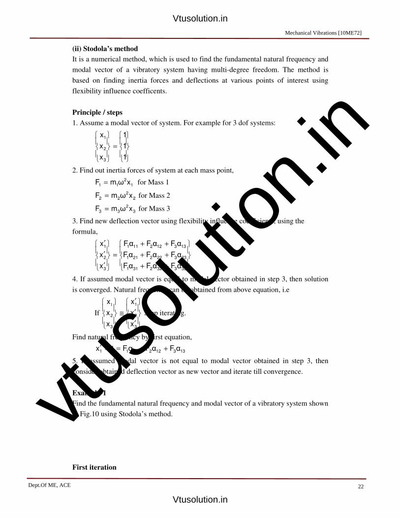
vtuso
lution
.inVTU e-learning Course ME65 Mechanical Vibrations
Prof. S. K. Kudari, Principal APS College of Engineering, Bengaluru-28.
22
(ii) Stodola’s method
It is a numerical method, which is used to find the fundamental natural frequency and
modal vector of a vibratory system having multi-degree freedom. The method is
based on finding inertia forces and deflections at various points of interest using
flexibility influence coefficents.
Principle / steps
1. Assume a modal vector of system. For example for 3 dof systems:
=
1
1
1
x
x
x
3
2
1
2. Find out inertia forces of system at each mass point,
1
2
11xωmF = for Mass 1
2
2
22xωmF = for Mass 2
3
2
33xωmF = for Mass 3
3. Find new deflection vector using flexibility influence coefficients, using the
formula,
++
++
++
=
′
′
′
333322311
233222211
133122111
3
2
1
αFαFαF
αFαFαF
αFαFαF
x
x
x
4. If assumed modal vector is equal to modal vector obtained in step 3, then solution
is converged. Natural frequency can be obtained from above equation, i.e
If
′
′
′
≅
3
2
1
3
2
x
x
x
x
x
x1
Stop iterating.
Find natural frequency by first equation,
1331221111αFαFαFx ++==′ 1
5. If assumed modal vector is not equal to modal vector obtained in step 3, then
consider obtained deflection vector as new vector and iterate till convergence.
Example-1
Find the fundamental natural frequency and modal vector of a vibratory system shown
in Fig.10 using Stodola’s method.
First iteration
Mechanical Vibrations [10ME72]
22Dept.Of ME, ACE
Vtusolution.in
Vtusolution.in
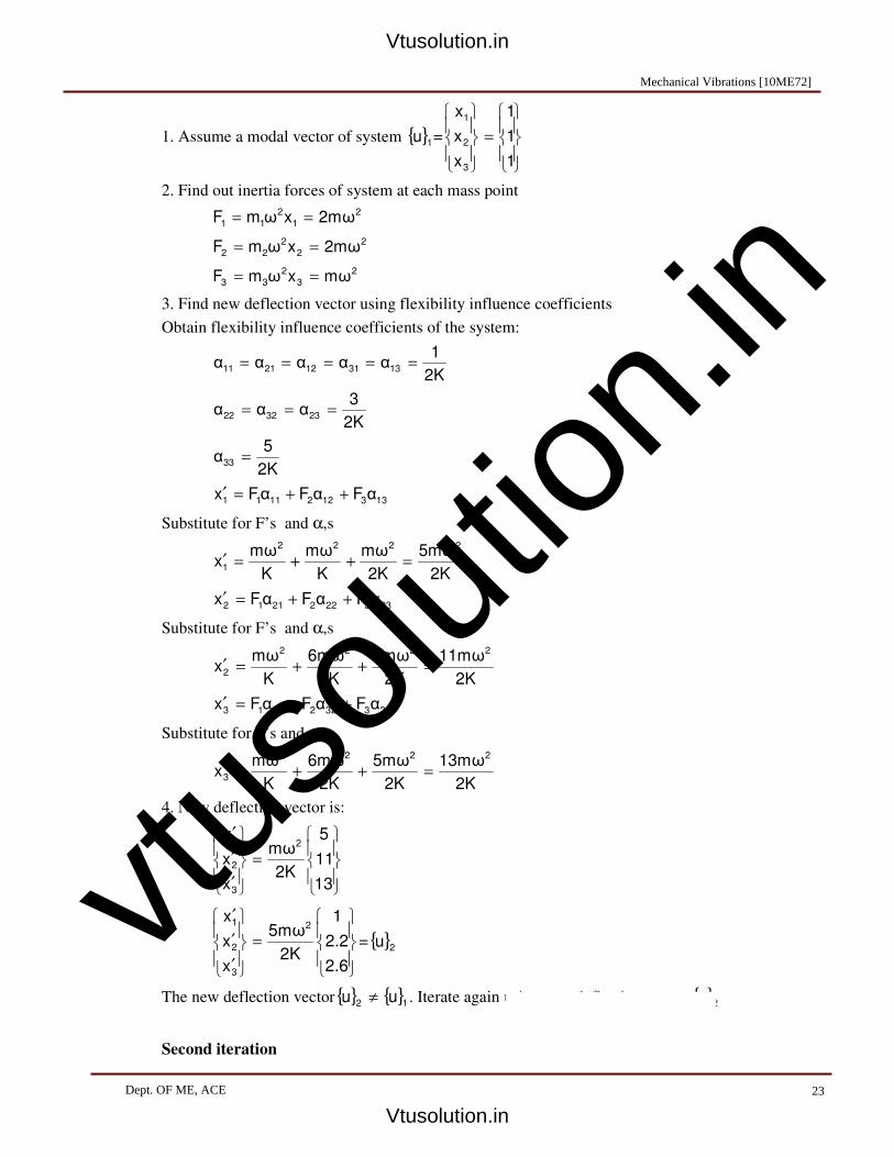
vtuso
lution
.inVTU e-learning Course ME65 Mechanical Vibrations
Prof. S. K. Kudari, Principal APS College of Engineering, Bengaluru-28.
23
1. Assume a modal vector of system { }1
u =
=
1
1
1
x
x
x
3
2
1
2. Find out inertia forces of system at each mass point
2
1
2
112mωxωmF ==
2
2
2
222mωxωmF ==
2
3
2
33mωxωmF ==
3. Find new deflection vector using flexibility influence coefficients
Obtain flexibility influence coefficients of the system:
2K
1ααααα
1331122111=====
2K
3ααα
233222===
2K
5α
33=
1331221111αFαFαFx ++=′
Substitute for F’s and α,s
2K
5mω
2K
mω
K
mω
K
mωx
2222
1=++=′
2332222112αFαFαFx ++=′
Substitute for F’s and α,s
2K
11mω
2K
3mω
2K
6mω
K
mωx
2222
2=++=′
3333223113αFαFαFx ++=′
Substitute for F’s and α,s
2K
13mω
2K
5mω
2K
6mω
K
mωx
2222
3=++=′
4. New deflection vector is:
=
′
′
′
13
11
5
2K
mω
x
x
x2
3
2
1
=
′
′
′
2.6
2.2
1
2K
5mω
x
x
x2
3
2
1
={ }2
u
The new deflection vector{ } { }12
uu ≠ . Iterate again using new deflection vector { }2
u
Second iteration
22Dept. OF ME, ACE
MechanicalMechanical Vibrations [10ME72]
23
Vtusolution.in
Vtusolution.in

vtuso
lution
.inVTU e-learning Course ME65 Mechanical Vibrations
Prof. S. K. Kudari, Principal APS College of Engineering, Bengaluru-28.
24
1. Initial vector of system { }2
u =
=
′
′
′
2.6
2.2
1
x
x
x
3
2
1
2. Find out inertia forces of system at each mass point
2
1
2
112mωxωmF =′=′
2
2
2
22mω4xωmF 4.=′=′
2
3
2
332.6mωxωmF =′=′
3. New deflection vector,
1331221111αFαFαFx ′+′+′=′′
Substitute for F’s and α,s
2K
9mω
2K
2.6mω
2K
4.4mω
K
mωx
2222
1=++=′′
2332222112αFαFαFx ′+′+′=′′
Substitute for F’s and α,s
2K
23mω
2K
7.8mω
2K
13.2mω
K
mωx
2222
2=++=′′
3333223113αFαFαFx ′+′+′=′′
Substitute for F’s and α,s
2K
28.2mω
2K
13mω
2K
13.2mω
K
mωx
2222
3=++=′′
4. New deflection vector is:
=
′′
′′
′′
28.2
23
9
2K
mω
x
x
x2
3
2
1
=
′′
′′
′′
3.13
2.55
1
2K
9mω
x
x
x2
3
2
1
={ }3
u
The new deflection vector{ } { }23
uu ≠ . Iterate again using new deflection vector{ }3
u
Third iteration
1. Initial vector of system { }3
u =
=
′′
′′
′′
3.13
2.55
1
x
x
x
3
2
1
2. Find out inertia forces of system at each mass point
2
1
2
112mωxωmF =′′=′′
2
2
2
225.1mωxωmF =′′=′′
Mechanical Vibrations [01ME72]
24Dept.Of ME, ACE
Vtusolution.in
Vtusolution.in

vtuso
lution
.inVTU e-learning Course ME65 Mechanical Vibrations
Prof. S. K. Kudari, Principal APS College of Engineering, Bengaluru-28.
25
3. new deflection vector,
1331221111αFαFαFx ′′+′′+′′=′′′
Substitute for F’s and α,s
2K
10.23mω
2K
3.13mω
2K
5.1mω
K
mωx
2222
1=++=′′′
2332222112αFαFαFx ′′+′′+′′=′′′
Substitute for F’s and α,s
2K
26.69mω
2K
9.39mω
2K
15.3mω
K
mωx
2222
2=++=′′′
3333223113αFαFαFx ′′+′′+′′=′′′
Substitute for F’s and α,s
2K
28.2mω
2K
16.5mω
2K
15.3mω
K
mωx
2222
3=++=′′′
4. New deflection vector is:
=
′′′
′′′
′′′
33.8
26.69
10.23
2K
mω
x
x
x2
3
2
1
=
′′′
′′′
′′′
3.30
2.60
1
2K
10.23mω
x
x
x2
3
2
1
={ }4
u
The new deflection vector { } { }34
uu ≅ stop Iterating
Fundamental natural frequency can be obtained by.
1=2K
10.23mω2
m
K0.44ω = rad/s
Modal vector is:
{ }
=
3.30
2.60
1
A1
2
3
2
333.13mωxωmF =′′=′′
Mechanical Vibrations [10ME72]
25Dept.Of ME, ACE
Vtusolution.in
Vtusolution.in
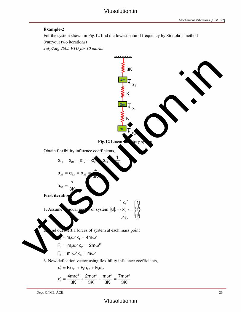
vtuso
lution
.inVTU e-learning Course ME65 Mechanical Vibrations
Prof. S. K. Kudari, Principal APS College of Engineering, Bengaluru-28.
26
Example-2
For the system shown in Fig.12 find the lowest natural frequency by Stodola’s method
(carryout two iterations)
July/Aug 2005 VTU for 10 marks
Obtain flexibility influence coefficients,
3K
1ααααα
1331122111=====
3K
4ααα
233222===
3K
7α
33=
First iteration
1. Assume a modal vector of system { }1
u =
=
1
1
1
x
x
x
3
2
1
2. Find out inertia forces of system at each mass point
2
1
2
114mωxωmF ==
2
2
2
222mωxωmF ==
2
3
2
33mωxωmF ==
3. New deflection vector using flexibility influence coefficients,
1331221111αFαFαFx ++=′
3K
7mω
3K
mω
3K
2mω
3K
4mωx
2222
1=++=′
4m
3K
2m
K
x1
x2
m
K
x3
Fig.12 Linear vibratory system
Mechanical Vibrations [10ME72]
26Dept. Of ME, ACE
Vtusolution.in
Vtusolution.in
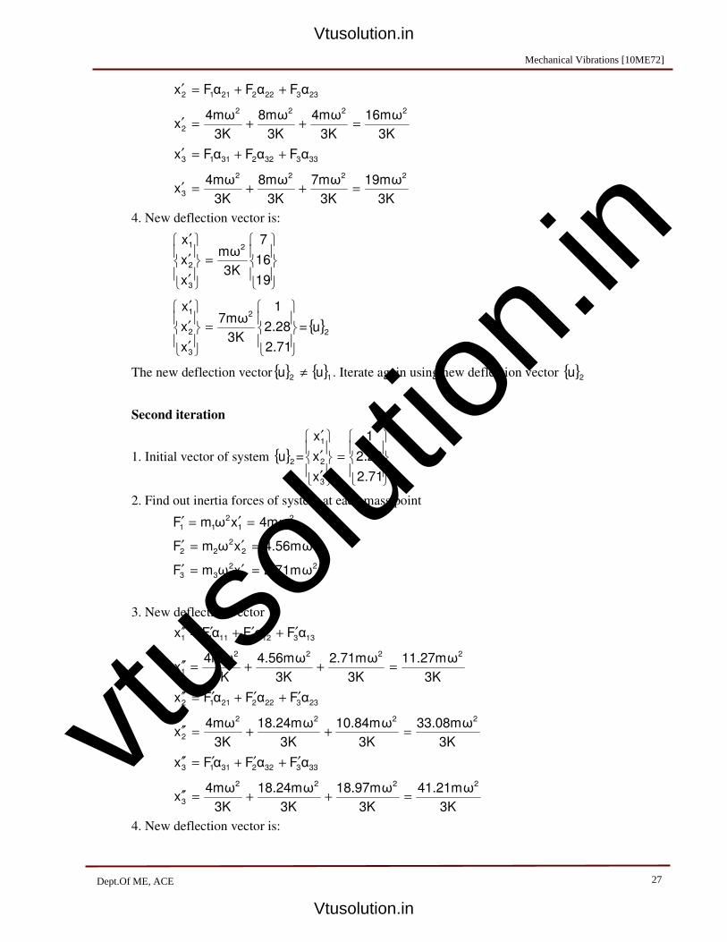
vtuso
lution
.inVTU e-learning Course ME65 Mechanical Vibrations
Prof. S. K. Kudari, Principal APS College of Engineering, Bengaluru-28.
27
2332222112αFαFαFx ++=′
3K
16mω
3K
4mω
3K
8mω
3K
4mωx
2222
2=++=′
3333223113αFαFαFx ++=′
3K
19mω
3K
7mω
3K
8mω
3K
4mωx
2222
3=++=′
4. New deflection vector is:
=
′
′
′
19
16
7
3K
mω
x
x
x2
3
2
1
=
′
′
′
2.71
2.28
1
3K
7mω
x
x
x2
3
2
1
={ }2
u
The new deflection vector{ } { }12
uu ≠ . Iterate again using new deflection vector { }2
u
Second iteration
1. Initial vector of system { }2
u =
=
′
′
′
2.71
2.28
1
x
x
x
3
2
1
2. Find out inertia forces of system at each mass point
2
1
2
114mωxωmF =′=′
2
2
2
224.56mωxωmF =′=′
2
3
2
332.71mωxωmF =′=′
3. New deflection vector
1331221111αFαFαFx ′+′+′=′′
3K
11.27mω
3K
2.71mω
3K
4.56mω
3K
4mωx
2222
1=++=′′
2332222112αFαFαFx ′+′+′=′′
3K
33.08mω
3K
10.84mω
3K
18.24mω
3K
4mωx
2222
2=++=′′
3333223113αFαFαFx ′+′+′=′′
3K
41.21mω
3K
18.97mω
3K
18.24mω
3K
4mωx
2222
3=++=′′
4. New deflection vector is:
Mechanical Vibrations [10ME72]
27Dept.Of ME, ACE
Vtusolution.in
Vtusolution.in

vtuso
lution
.inVTU e-learning Course ME65 Mechanical Vibrations
Prof. S. K. Kudari, Principal APS College of Engineering, Bengaluru-28.
28
=
′′
′′
′′
41.21
33.08
11.27
3K
mω
x
x
x2
3
2
1
=
′′
′′
′′
3.65
2.93
1
K
3.75mω
x
x
x2
3
2
1
={ }3
u
Stop Iterating as it is asked to carry only two iterations. The Fundamental natural
frequency can be calculated by,
12K
3.75mω2
=
m
K0.52ω =
Modal vector,
{ }
=
3.65
2.93
1
A1
Disadvantage of Stodola’s method
Main drawback of Stodola’s method is that the method can be used to find only
fundamental natural frequency and modal vector of vibratory systems. This method is
not popular because of this reason.
Mechanical Vibrations [10ME72]
28Dept.Of ME, ACE
Vtusolution.in
Vtusolution.in

vtuso
lution
.inVTU e-learning Course ME65 Mechanical Vibrations
Prof. S. K. Kudari, Principal APS College of Engineering, Bengaluru-28.
29
(iii) Holzar’s method
It is an iterative method, used to find the natural frequencies and modal vector of a
vibratory system having multi-degree freedom.
Principle
Consider a multi dof semi-definite torsional semi-definite system as shown in Fig.13.
The Eqns. of motions of the system are:
0θ(θKθJ21111
=−+ )&&
0θ(θKθ(θKθJ32212122
=−+−+ ))&&
0θ(θKθ(θKθJ43323233
=−+−+ ))&&
0θ(θKθJ34344
=−+ )&&
The Motion is harmonic,
( )ωtsinφθii
= (17)
where i=1,2,3,4
Substitute above Eqn.(17) in Eqns. of motion, we get,
)φ(φKφJω21111
2 −= (18)
)φ(φK)φ(φKφJω32212122
2 −+−=
)φ(φK)φ(φKφJω43323233
2 −+−=
)φ(φKφJω34344
2 −+ (19)
Add above Eqns. (18) to (19), we get
0φJω4
1i
ii
2 =∑=
For n dof system the above Eqn changes to,
0φJωn
1i
ii
2 =∑=
(20)
The above equation indicates that sum of inertia torques (torsional systems) or inertia
forces (linear systems) is equal to zero for semi-definite systems.
θ1 K1 θ2 θ3 K2 K3 θ4
J4 J3
J2 J1
Fig.13 A torsional semi-definite system
Mechanical Vibrations[10ME72]
29Dept. Of ME, ACE
Vtusolution.in
Vtusolution.in

vtuso
lution
.inVTU e-learning Course ME65 Mechanical Vibrations
Prof. S. K. Kudari, Principal APS College of Engineering, Bengaluru-28.
30
In Eqn. (20) ω and φi both are unknowns. Using this Eqn. one can obtain natural
frequencies and modal vectors by assuming a trial frequency ω and amplitude φ1 so
that the above Eqn is satisfied.
Steps involved
1. Assume magnitude of a trial frequency ω
2. Assume amplitude of first disc/mass (for simplicity assume φ1=1
3. Calculate the amplitude of second disc/mass φ2 from first Eqn. of motion
0)φ(φKφJω21111
2 =−=
1
11
2
12K
φJωφφ −=
4. Similarly calculate the amplitude of third disc/mass φ3 from second Eqn. of motion.
0)φ(φK)φ(φKφJω32212122
2 =−+−=
0)φ(φK)φK
φJω(φKφJω
3221
1
11
2
1122
2 =−+−−=
0)φ(φKφJωφJω32211
2
22
2 =−+−=
22
2
11
2
322φJωφJω)φ(φK +=−
2
22
2
11
2
23K
φJωφJω-φφ
+= (21)
The Eqn (21) can be written as:
2
2
1i
2
ii
23K
ωφJ
-φφ∑
==
5. Similarly calculate the amplitude of nth disc/mass φn from (n-1)th Eqn. of motion
is:
n
n
1i
2
ii
1-nnK
ωφJ
-φφ∑
==
6. Substitute all computed φi values in basic constraint Eqn.
0φJωn
1i
ii
2 =∑=
7. If the above Eqn. is satisfied, then assumed ω is the natural frequency, if the Eqn is
not satisfied, then assume another magnitude of ω and follow the same steps.
For ease of computations, Prepare the following table, this facilitates the calculations.
Table-1. Holzar’s Table
MMechanical Vibrations [10ME72]
30Dept. Of ME, ACE
Vtusolution.in
Vtusolution.in

vtuso
lution
.inVTU e-learning Course ME65 Mechanical Vibrations
Prof. S. K. Kudari, Principal APS College of Engineering, Bengaluru-28.
31
1 2 3 4 5 6 7 8
ω
S No J φ Jω
2φ
K
Example-1
For the system shown in the Fig.16, obtain natural frequencies using Holzar’s method.
Make a table as given by Table-1, for iterations, follow the steps discussed earlier.
Assume ω from lower value to a higher value in proper steps.
Table-2. Holzar’s Table for Example-1
1 2 3 4 5 6 7 8
ω
S No J φ Jω
2φ
K
I-iteration
0.25
1 1 1 0.0625 0.0625 1 0.0625
2 1 0.9375 0.0585 0.121 1 0.121
3 1 0.816 0.051 0.172
II-iteration
0.50
1 1 1 0.25 0.25 1 0.25
2 1 0.75 0.19 0.44 1 0.44
3 1 0.31 0.07 0.51
III-iteration
0.75
1 1 1 0.56 0.56 1 0.56
2 1 0.44 0.24 0.80 1 0.80
3 1 -0.36 -0.20 0.60
IV-iteration
1.00 1 1 1 1 1 1 1
2 1 0 0 1 1 1
∑ φ2Jω ∑ φ2
JωK
1
θ1 K1 θ2 θ3 K2
J3 J2 J1
Fig.14 A torsional semi-definite system
∑ φ2Jω ∑ φ2
JωK
1
Mechanical Vibrations[10ME72]
31Dept.Of ME, ACE
Vtusolution.in
Vtusolution.in

vtuso
lution
.inVTU e-learning Course ME65 Mechanical Vibrations
Prof. S. K. Kudari, Principal APS College of Engineering, Bengaluru-28.
32
3 1 -1 -1 0
V-iteration
1.25
1 1 1 1.56 1.56 1 1.56
2 1 -0.56 -0.87 0.69 1 0.69
3 1 -1.25 -1.95 -1.26
VI-iteration
1.50
1 1 1 2.25 2.25 1 2.25
2 1 -1.25 -2.82 -0.57 1 -0.57
3 1 -0.68 -1.53 -2.10
VII-iteration
1.75
1 1 1 3.06 3.06 1 3.06
2 1 -2.06 -6.30 -3.24 1 -3.24
3 1 1.18 3.60 0.36
Table.3 Iteration summary table
ω
0 0
0.25 0.17
0.5 0.51
0.75 0.6
1 0
1.25 -1.26
1.5 -2.1
1.75 0.36
∑ φ2Jω
Mechanical Vibrations[10ME72]
32Dept. Of ME, ACE
Vtusolution.in
Vtusolution.in

vtuso
lution
.inVTU e-learning Course ME65 Mechanical Vibrations
Prof. S. K. Kudari, Principal APS College of Engineering, Bengaluru-28.
33
The values in above table are plotted in Fig.15.
From the above Graph, the values of natural frequencies are:
rad/s 1.71ω
rad/s 1ω
rad/s 0ω
3
2
1
=
=
=
Definite systems
The procedure discussed earlier is valid for semi-definite systems. If a system is
definite the basic equation Eqn. (20) is not valid. It is well-known that for definite
systems, deflection at fixed point is always ZERO. This principle is used to obtain the
natural frequencies of the system by iterative process. The Example-2 demonstrates
the method.
0.00 0.25 0.50 0.75 1.00 1.25 1.50 1.75 2.00
-2.5
-2.0
-1.5
-1.0
-0.5
0.0
0.5
1.0
1.5
∑ φ2Jω
Frequency, ω
Fig.15. Holzar’s plot of Table-3
Mechanical Vibrations [10ME72]
33Dept.Of ME, ACE
Vtusolution.in
Vtusolution.in
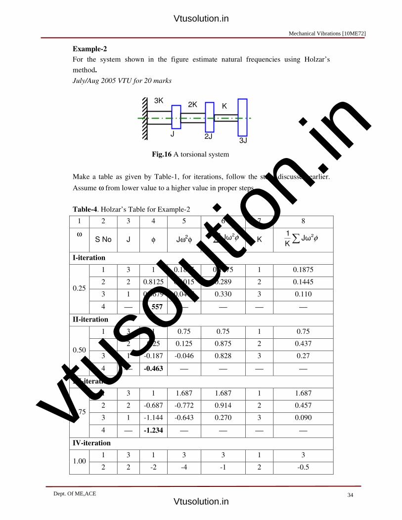
vtuso
lution
.inVTU e-learning Course ME65 Mechanical Vibrations
Prof. S. K. Kudari, Principal APS College of Engineering, Bengaluru-28.
34
Example-2
For the system shown in the figure estimate natural frequencies using Holzar’s
method.
July/Aug 2005 VTU for 20 marks
Make a table as given by Table-1, for iterations, follow the steps discussed earlier.
Assume ω from lower value to a higher value in proper steps.
Table-4. Holzar’s Table for Example-2
1 2 3 4 5 6 7 8
ω
S No J φ Jω
2φ
K
I-iteration
0.25
1 3 1 0.1875 0.1875 1 0.1875
2 2 0.8125 0.1015 0.289 2 0.1445
3 1 0.6679 0.0417 0.330 3 0.110
4 0. 557
II-iteration
0.50
1 3 1 0.75 0.75 1 0.75
2 2 0.25 0.125 0.875 2 0.437
3 1 -0.187 -0.046 0.828 3 0.27
4 -0.463
III-iteration
0.75
1 3 1 1.687 1.687 1 1.687
2 2 -0.687 -0.772 0.914 2 0.457
3 1 -1.144 -0.643 0.270 3 0.090
4 -1.234
IV-iteration
1.00 1 3 1 3 3 1 3
2 2 -2 -4 -1 2 -0.5
J 2J
3K 2K K
3J
Fig.16 A torsional system
∑ φ2Jω ∑ φ2
JωK
1
Mechanical Vibrations [10ME72]
34Dept. Of ME,ACE
Vtusolution.in
Vtusolution.in

vtuso
lution
.inVTU e-learning Course ME65 Mechanical Vibrations
Prof. S. K. Kudari, Principal APS College of Engineering, Bengaluru-28.
35
3 1 -1.5 -1.5 -2.5 3 -0.833
4 -0.667
V-iteration
1.25
1 3 1 4.687 4.687 1 4.687
2 2 -3.687 -11.521 -6.825 2 -3.412
3 1 -0.274 -0.154 -6.979 3 -2.326
4 2.172
VI-iteration
1.50
1 3 1 6.75 6.75 1 6.75
2 2 -5.75 -25.875 -19.125 2 -9.562
3 1 3.31 8.572 -10.552 3 -3.517
4 7.327
1 2 3 4 5 6 7 8
ω
S No J φ Jω
2φ
K
VII-iteration
1.75
1 3 1 9.18 9.18 1 9.18
2 2 -8.18 -50.06 -40.88 2 -20.44
3 1 12.260 37.515 -3.364 3 -1.121
4 13.38
VIII-iteration
2.0
1 3 1 12 12 1 12
2 2 -11 -88 -76 2 -38
3 1 -27 108 32 3 10.66
4 16.33
IX-iteration
2.5
1 3 1 18.75 18.75 1 18.75
2 2 -17.75 -221.87 -203.12 2 -101.56
3 1 83.81 523.82 320.70 3 106.90
4 -23.09
∑ φ2Jω ∑ φ2
JωK
1
Mechanical Vibrations[10ME72]
35Dept.Of ME, ACE
Vtusolution.in
Vtusolution.in

vtuso
lution
.inVTU e-learning Course ME65 Mechanical Vibrations
Prof. S. K. Kudari, Principal APS College of Engineering, Bengaluru-28.
36
Table.5 Iteration summary table
ω φ4
0 0
0.25 0.557
0.5 -0.463
0.75 -1.234
1 -0.667
1.25 2.172
1.5 7.372
1.75 13.38
2 16.33
2.5 -23.09
The values in above table are plotted in Fig.17.
From the above Graph, the values of natural frequencies are:
rad/s 2.30ω
rad/s 1.15ω
rad/s 0.35ω
3
2
1
=
=
=
0.0 0.5 1.0 1.5 2.0 2.5
-20
-10
0
10
20
Dis
pla
ce
me
nt,
φ4
Frequency,ω
1ω
2ω
3ω
Fig.17. Holzar’s plot of Table-5
Mechanical Vibrations [10ME72]
36Dept. Of ME, ACE
Vtusolution.in
Vtusolution.in

vtuso
lution
.in
1
Unit - 7
Vibration of Continuous System
Dr. T. Jagadish. Professor for Post Graduation, Department of Mechanical Engineering, Bangalore
Institute of Technology, Bangalore
Continuous systems are tore which have continuously distributed mass and Elasticity. These continuous
systems are assumed to be homogeneous and isotropic obeying hook law within the elastic limit. Since to
specify the position of every point in the continuous systems an infinite number of coordinates is required
therefore a continuous systems is considered to have infinite number of degrees of freedom. Thus there will
be infinite natural frequencies
Free vibration of continuous system is sum of the principal or normal modes. For the normal mode
vibration, every particle of the body performs simple harmonic motion at the frequency corresponding to
the particular root of the frequency equation, each particles passing simultaneously through its respective
equilibrium position. If the elastic curve resulting due to vibration motion starts coinciding exactly with
one of the normal modes, only that normal mode will be produced. If the elastic curve of the system under
which the vibration is started, is identical to any one of the principal mode shapes, then the system will
vibrate only in that principal mode.
Vibration of String.
A string stretched between two support is shown in figure-1 is an infinite degree of freedom system.
Figure-1
dx X
Y
y
x dx
T
θθθθ
θθθθ + (δ + (δ + (δ + (δθθθθ/δ/δ/δ/δx) dx
T
UNIT - 7
MULTIDEGREE VIBRATIONS SYSTEMSMULTI DEGREE FREEDOM OFSYSTEMS
Mechanical Vibrations [10ME72]
Dept. Of ME, ACE
UNIT - 8
MODAL ANALYSIS AND CONDITION MONITORING
Vtusolution.in
Vtusolution.in

vtuso
lution
.in
2
Let the tension T in the string be large so that for small displacement or amplitude the tension in the
string remains constant throughout the string. Consider an element of length dx at a distance ‘x’ from the
left end. At any instant of time the element of the string be displaced through a distance ‘y’ from the
equilibrium position. Then the tension at both the ends of this element is ‘T’. If θ the angle at the left end
of the element makes with the horizontal x- axis then the angle at the right end of the element is
θ + (δθ/δx)dx
The components of these two tensions at the ends of the element along x-axis balance each others.
The components along Y – axis � ��� �� � � �� � � sin � Since θ is small
� � �� � �� �� � �� � � �� �� � �1�
If ‘ρ' is mass per unit length, then the mass of the element is ‘ρdx’ and the differential equation of motion
along Y-axis according to Newton’s second law of motion is,
Mass x Acceleration = Sum of all the forces.
��� ������ � � �� �� Therefore � ���
��� � � ��
But we know slope � � ��� then we have
� ������ � � ����� or ������ �
��
������ or
����� �
�� �⁄ ������
����� �
���
������ --- (2)
Where � !� �⁄ ------ (3) is the velocity of wave propagation along the string. Solution of equation (2)
can be obtained by assuming Y through separation of variables to be a product of two functions in the
form. " ��, $� � % ��� & �$� � � � ��4�
()"(�) � & (
)"(�) *��
()"($) � % (
)"($) � � � �5�
Substituting equation (5) in to equation (2) we have
Mechanical Vibrations [10ME72]
Dept. Of ME, ACE 2
Vtusolution.in
Vtusolution.in

vtuso
lution
.in
3
& ����� � ,��
��-��� ./
�,
����� � �
-�� ��-���
0�,����� �
�-
��-��� ---- (6)
Left hand side of equation (6) is a function of x alone and the right hand side is a function of t alone. These
two can only be equal if each one of these expression is a constant. This constant may be positive, zero or
negative. If it is a positive constant or zero then there is no vibratory motion. Hence this constant has to be
negative constant and equal to -�2
Then 0�,����� �
�-
��-��� � � ) � � � � � �7�
)%()"(�) � 2
) � 0 *�� 1& ()&($) � 2) � 0
()"(�) � �4� �) % � 0 *�� (
)&($) � 2) � 0 � � � �� �8�
With the general solution Y � A sin 89� � : ;.< 89� � � � ��9�
G � D sin $ � @;.< $ � � � ��10� Substituting equation (9) and (10) into equation (4) we have
" ��, $� � �A sin 40� � : ;.< 40� �D sin $ � @;.< $� � � � �11�
Since 2 can have infinite values, being an infinite degree of freedom system the general solution can be
written as
" ��, $� � ∑ BAisin 8C9 � � :� ;.< 8C9 � D�Disin �$ � @�;.< �$� � ��11�∞EF�
The arbitrary constant A, B, D and E have to be determined from the boundary condition and the initial
conditions.
For the string of length ‘L’ stretched between two fixed points. The boundary conditions are
y(0,t) = y(L, t) = 0
The condition y (0, t) = 0 will require B = 0 so the solution will be
Mechanical Vibrations [10ME72]
Dept. Of ME, ACE
Vtusolution.in
Vtusolution.in
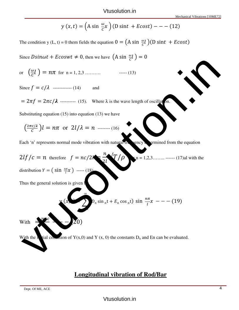
vtuso
lution
.in
4
" ��, $� � �A sin 40� �D sin $ � @;.< $� � � � �12�
The condition y (L, t) = 0 them fields the equation 0 � BA sin 89H D�D sin $ � @;.< $�
Since I<��2$ � @;.<J$ K 0, then we have BA sin 89H D � 0
or B89H D � �L for n = 1, 2,3 ………. ----- (13)
Since M � ;/O ------------ (14) and
� 2LM � 2L;/P ---------- (15). Where λ is the wave length of oscillation.
Substituting equation (15) into equation (13) we have
B�QR/P9 DH � �L or 2H/O � � -------- (16)
Each ‘n’ represents normal mode vibration with natural frequency determined from the equation
2HM/; � � therefore M � �;/2H = S)T√�/V for n = 1,2,3…….. ------ (17)al with the
distribution % � B sin �LH � D ----- (18)
Thus the general solution is given by
" ��, $� � W�I� sin �t � @� cos �t�∞
��1 sin S\T � � � � �19�
With � S\�T � � � �20�
With the initial condition of Y(x,0) and Y (x, 0) the constants Dn and En can be evaluated.
Longitudinal vibration of Rod/Bar
Mechanical Vibrations [10ME72]
Dept. Of ME, ACE
Vtusolution.in
Vtusolution.in
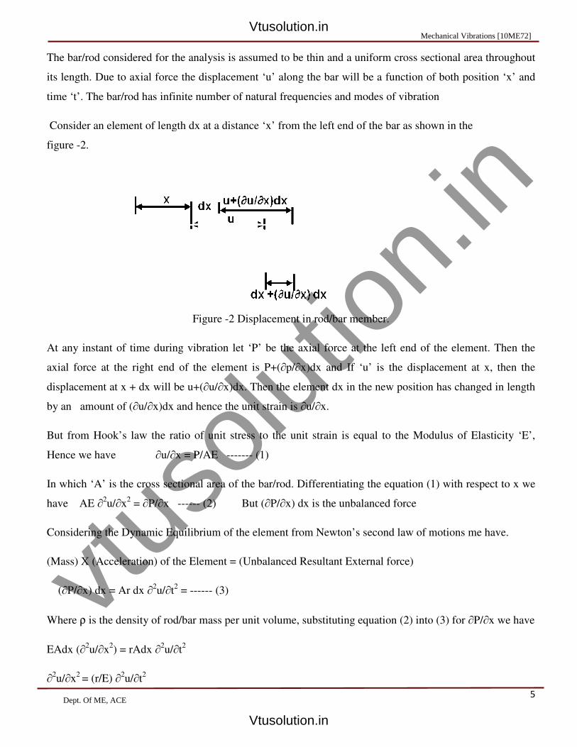
vtuso
lution
.in
The bar/rod considered for the analysis is assumed to be thin and a uniform cross sectional area throughout
its length. Due to axial force the displacement ‘u’ along the bar will be a function of both position ‘x’ and
time ‘t’. The bar/rod has infinite number of natural frequencies and modes of vibration
Consider an element of length dx at a distance ‘x’ from the left end of the bar as shown in the
figure -2.
Figure
At any instant of time during vibration let ‘P’ be the axial force at the left end of the element. Then the
axial force at the right end of the element is P+(
displacement at x + dx will be u+(∂u/
by an amount of (∂u/∂x)dx and hence the unit strain is
But from Hook’s law the ratio of unit stress to the unit strain is equal to the Modulus of Elasticity ‘E
Hence we have ∂u/∂x = P/AE
In which ‘A’ is the cross sectional area of the bar/rod.
have AE ∂2u/∂x2
= ∂P/∂x ------ (2)
Considering the Dynamic Equilibrium of the element from Newton’s second law of motions me have.
(Mass) X (Acceleration) of the Element = (Unbalanced Resultant External force)
(∂P/∂x) dx = Ar dx ∂2u/∂t2
= ------ (3)
Where ρ is the density of rod/bar mass per unit volume, substituting equation
EAdx (∂2u/∂x2
) = rAdx ∂2u/∂t2
∂2u/∂x2
= (r/E) ∂2u/∂t2
The bar/rod considered for the analysis is assumed to be thin and a uniform cross sectional area throughout
its length. Due to axial force the displacement ‘u’ along the bar will be a function of both position ‘x’ and
bar/rod has infinite number of natural frequencies and modes of vibration
Consider an element of length dx at a distance ‘x’ from the left end of the bar as shown in the
igure -2 Displacement in rod/bar member.
At any instant of time during vibration let ‘P’ be the axial force at the left end of the element. Then the
axial force at the right end of the element is P+(∂p/∂x)dx and If ‘u’ is the displacement at x, then the
u/∂x)dx. Then the element dx in the new position has changed in length
x)dx and hence the unit strain is ∂u/∂x.
But from Hook’s law the ratio of unit stress to the unit strain is equal to the Modulus of Elasticity ‘E
x = P/AE ------- (1)
‘A’ is the cross sectional area of the bar/rod. Differentiating the equation (1) w
(2) But (∂P/∂x) dx is the unbalanced force
Considering the Dynamic Equilibrium of the element from Newton’s second law of motions me have.
(Mass) X (Acceleration) of the Element = (Unbalanced Resultant External force)
(3)
ass per unit volume, substituting equation (2) into (3)
5
The bar/rod considered for the analysis is assumed to be thin and a uniform cross sectional area throughout
its length. Due to axial force the displacement ‘u’ along the bar will be a function of both position ‘x’ and
bar/rod has infinite number of natural frequencies and modes of vibration
Consider an element of length dx at a distance ‘x’ from the left end of the bar as shown in the
At any instant of time during vibration let ‘P’ be the axial force at the left end of the element. Then the
x)dx and If ‘u’ is the displacement at x, then the
x)dx. Then the element dx in the new position has changed in length
But from Hook’s law the ratio of unit stress to the unit strain is equal to the Modulus of Elasticity ‘E’,
Differentiating the equation (1) with respect to x we
Considering the Dynamic Equilibrium of the element from Newton’s second law of motions me have.
(2) into (3) for ∂P/∂x we have
Mechanical Vibrations [10ME72]
Dept. Of ME, ACE
Vtusolution.in
Vtusolution.in
vtuso
lution
.in
6
∂2u/∂x2
= [1/(E/r)] ∂2u/∂t2
--------------- (4)
∂2u/∂x2
= (1/c2) ∂2
u/∂t2 --------------- (5)
Where c = √(E/r) ------ (6) is the velocity of propagation of the displacement or stress wave in the rod/bar.
Solution of equation (5) can be obtained by assuming u through separation of variables to be a product of
two functions in the form u(x, t) = U(x) G(t) ------ (7)
∂2u/∂x2
=G(∂2U/∂x2
) and ∂2u/∂t2
=U(∂2G/∂t2
) --(8)
Substituting equation (8) in to equation (5) we have G(∂2U/∂x2
) = (U/c2)(∂2
G/∂t2)
Then (c2/U)(∂2
U/∂x2) = (1/G)(∂2
G/∂t2) ----- (9)
Left hand side of equation (9) is a function of x alone and the right hand side is a function of t alone. These
two can only be equal if each one of these expression is a constant.
This constant may be positive, zero or negative. If it is a positive constant or zero then there is no vibratory
motion. Hence this constant have to be negative constant and equal to - w2 . Then we have
(c2/U)(∂2
U/∂x2)=(1/G)(∂2
G/∂t2)= - ω
2 ------- (10)
(c2/U)(∂2
U/∂x2)= - w
2 and (1/G)(∂2
G/∂t2)= - ω
2
∂2U/∂x2
+(ω/c)2U = 0 and ∂2
G/∂t2+ω
2G = 0 - (11)
With the general solution U = Asin(ω/c)x + Bcos(ω/c)x ----- (12) G = Dsinωt + Ecosωt ------ (13)
Substituting equation (12) and (13) into equation (7) we have
u(x, t) = [Asin(ω/c)x + Bcos(ω/c)x] * [Dsinωt + Ecosωt] --------- (14)
Since ω can have infinite values, as the system being an infinite degree of freedom the general solution can
be written as
u(x, t) =∑i∞
=1[Aisin(ωi/c)x + Bicos(ωi/c)x] [Disinωit + Eicosωit ] -------- (15)
The arbitrary constant A, B, D and E have to be determined from the boundary condition and the initial
conditions.
Mechanical Vibrations [10ME72]
Dept. Of ME, ACE
Vtusolution.in
Vtusolution.in

vtuso
lution
.in
Example:
Determine the natural frequencies and mode shape of a bar/rod when both the ends are free
Solution: When the bar/rod with both the ends being free then the stress and strain at the ends are zero
The boundary conditions are ∂u/∂x = 0 at x= 0 and x= L
u(x, t) = [Asin(ω/c)x + Bcos(ω/c)x] [Dsin
∂u/∂x = [(Aω/c)cos(ω/c)x + (Bω/c)sin(
(∂u/∂x)x=0=(Aω/c)[Dsinwt + Ecosωt] = 0
(∂u/∂x) x=L = (ω/c)[Acos(ωL/c) + Bsin(
Since the equation (4) and (5) must be true for any time ‘t’
From equation (4) A must be equal to zero.
equation (5) is satisfied only when sin(
Since c = √(E/ρ) then we have ωnL
since the natural frequency is fn = ωn
fn = (n/2L) √(E/ρ) ------------- (7)
Each ‘n’ represents normal mode vibration with natural frequency ‘f
equation (7).
Torsional vibration
Consider an element of length dx at a distance x from one end of the shaft as shown in the figure
Determine the natural frequencies and mode shape of a bar/rod when both the ends are free
When the bar/rod with both the ends being free then the stress and strain at the ends are zero
∂x = 0 at x= 0 and x= L ------- (1)
/c)x] [Dsinωt + Ecosωt] ------------ (2)
/c)sin(ω/c)x] [Dsinωt + Ecosωt] ------------ (3)
t] = 0 --- (4)
L/c) + Bsin(ωL/c)] [Dsinωt + Ecosωt] = 0 ------ (5)
Since the equation (4) and (5) must be true for any time ‘t’
From equation (4) A must be equal to zero. Since B must be finite value in order to have vibration then
sin(ωnL/c) = 0 or ωnL/c =sin-1
(0) = nπ
L√(ρ/E) = nπ Thus ωn = (nπ/L) √(E/ρ) ------
n/2π = [(nπ/L) √(E/ρ)]/ 2π
Each ‘n’ represents normal mode vibration with natural frequency ‘fn’ determined from the
sional vibration of circular shaft.
Consider an element of length dx at a distance x from one end of the shaft as shown in the figure
7
Determine the natural frequencies and mode shape of a bar/rod when both the ends are free.
When the bar/rod with both the ends being free then the stress and strain at the ends are zero
Since B must be finite value in order to have vibration then
(6)
’ determined from the
Consider an element of length dx at a distance x from one end of the shaft as shown in the figure -3
Mechanical Vibrations [10ME72]
Dept. Of ME, ACE 7
Vtusolution.in
Vtusolution.in

vtuso
lution
.in
8
Figure -3 Torque acting on the element of the circular shaft
At any given instant of time during vibration let T be the torque at left end of the element. Then the torque
at the right end of the element is given by T+(∂T/∂x)dx.
If θ is the angular twist of the shaft at the distance x, then θ+(∂θ/∂x)dx is the angular twist of the
shaft at the distance x+dx. Therefore the angular twist in the element of length dx is (∂θ/∂x)dx.
If ‘J’ is the polar moment of inertia of the shaft and ‘G’ the modulus of rigidity then the angular twist in the
element of length dx is given by torsion formula
dθ = (T/GJ) dx ------- (1) or GJ(dθ/dx) = T ------- (2)
Differentiating with respect to x we have GJ(d2θ/dx
2) = dT/dx ------- (3)
In which GJ is the torsional stiffness of the shaft. Since the torque on the two face of the element being T
and T+(∂T/∂x)dx the net torque on the element will be (∂T/∂x)dx --- (4)
Substituting equation (3) for ∂T/∂x in to equation (4) we have (∂T/∂x)dx = GJ(∂2θ/∂x2
)dx ------- (5)
Considering the dynamic equilibrium of the element one can obtain the equation of motion by equating the
product of mass moment of inertia ‘Jρdx’ and the acceleration ‘∂2θ/∂t2
’ to the net torque acting on the
element we have.
(Jρdx) ∂2θ/∂t2
= GJ(∂2θ/∂x2
)dx
∂2θ/∂t2
= (G/ρ)(∂2θ/∂x2
) or
∂2θ/∂x2
= (ρ/G) ∂2θ/∂t2
∂2θ/∂x2
= [1/(G/ρ)] ∂2θ/∂t2
∂2θ/∂x2
= (1/c2) ∂2
θ/∂t2 --------- (6)
Where c = √(G/ρ) ------ (7) is the velocity of wave propagation in which r is the density of the shaft in
mass per unit volume.
Mechanical Vibrations[10ME72]
Dept. Of ME, ACE
Vtusolution.in
Vtusolution.in
vtuso
lution
.in
9
Solution of equation (6) can be obtained by assuming q through separation of variables to be a product of
two functions in the form. θ(x, t) = Θ(x) G(t) ------ (7)
∂2θ/∂x2
=G(∂2Θ/∂x2) and ∂2
θ/∂t2=Θ(∂2
G/∂t2)---(8)
Substituting equation (8) in to equation (6) we have G(∂2Θ/∂x2) = (Θ/c
2)(∂2
G/∂t2)
Then (c2/Θ)(∂2Θ/∂x2
) = (1/G)(∂2G/∂t2
) ----- (9)
Left hand side of equation (9) is a function of ‘Θ’ alone and the right hand side is a function of ‘t’ alone.
These two can only be equal if each one of these expression is a constant. This constant may be positive,
zero or negative. If it is a positive constant or zero then there is no vibratory motion. Hence this constant
has to be negative constant and equal to - ω2
(c2/Θ)(∂2Θ/∂x2
)=(1/G)(∂2G/∂t2
) = -ω2
-- (10)
(c2/Θ)(∂2Θ/∂x2
)= - ω2
and (1/G)(∂2G/∂t2
)= - ω2
∂2Θ/∂x2+(ω/c)
2Θ = 0 and ∂2G/∂t2
+ω2G = 0--(11)
With the general solution Θ = Asin(ω/c)x + Bcos(ω/c)x ----- (12) G = Dsinωt + Ecosωt ------ (13)
Substituting equation (12) and (13) into equation (7) we have
θ(x, t) = [Asin(ω/c)x + Bcos(ω/c)x] [Dsinωt + Ecosωt] --------- (14)
Since ω can have infinite values, as the system being an infinite degree of freedom the general solution can
be written as
θ(x, t) =∑i∞
=1[Aisin(ωi/c)x + Bicos(ωi/c)x] [Disinωit + Eicosωit ] -------- (15)
The arbitrary constant A, B, D and E have to be determined from the boundary condition and the initial
conditions.
Lateral Vibration of beams
To derive the differential equation of motion for lateral vibration of beams one has to consider the forces
and moments acting on the beam. Let V and M are the shear forces and bending moments respectively
acting on the beam with p(x) represents the intensity of lateral loading per unit length of the beam.
Mechanical Vibrations[10ME72]
Dept. Of ME, ACE
Vtusolution.in
Vtusolution.in

vtuso
lution
.in
10
Consider a beam of length ‘L’ and moment of inerter ‘I’ subjected to distributed lateral load of p(x) N per
unit length. At any section x-x at a distance x from one end consider an element of length dx as shown in
the figure-4. The force and the moments acting on the element of length dx are as shown in the figure-5
Figure-4 Beam Figure-5 Force and Moments
For static equilibrium the summation of the forces and moment should be equal to zero. Thus summing the
vertical force in the Y – direction and equating to zero we have
V + p(x) dx – [V +(∂V/∂x) dx] = 0
[p(x) - (∂V/∂x)] dx = 0 since dx ≠ 0
p(x) - (∂V/∂x) = 0 or ∂V/∂x = p(x) ---- (1)
Which state that the rate of change of shear force along the length of the beam is equal to the load per unit
length.
Summation of the moment about any point should be equal to zero. Thus summing the moments about the
right bottom corner of the element considering the clockwise moment as positive we have
M + p(x) dx2/2 + V dx – [M +(∂M/∂x) dx] = 0 or p(x) dx
2/2 + V dx – (∂M/∂x) dx = 0
Since dx is small neglecting the higher order terms we have
[V – (∂M/∂x)] dx = 0 Since dx ≠ 0 we have
V – (∂M/∂x) = 0 ∂M/∂x = V ----- (2)
Which state that the rate of change of bending moment along the length of the beam is equal to the shear
force.
From equation (1) and (2) we have ∂2M/∂x2
= ∂V/∂x = p(x) ----- (3)
Mechanical Vibrations[10ME72]
Dept.. Of ME, ACE
Vtusolution.in
Vtusolution.in

vtuso
lution
.in
11
But we known that the bending moment is related to curvature by flexure formula and for the coordinates
indicated we have EI(d2y/dx
2) = M ----- (4)
Substituting equation (4) into equation (3) we have ∂2[EI(d
2y/dx
2) ]/∂x2
= p(x)
EI (d4y/dx
4) = p(x) ----- (5)
For the dynamic equilibrium when the beam is having transverse vibrations about its static equilibrium
position under its own weight and due to the distributed load per unit length must be equal to the inertia
load due its mass and acceleration. By assuming harmonic motion the inertia force ρωy2
is in the same
direction as that of the distributed load p(x).
Thus we have p(x) = ρω2y ------ (6)
In which ρ is the mass density per unit length of the beam. Thus substituting equation (6) into equation (5)
for p(x) we have EI(d4y/dx
4) = ρω
2y or EI(d
4y/dx
4) - ρω
2y = 0 ------ (7)
If the flexural rigidity EI is constant then equation (7) can be written as d4y/dx
4 - (ρω
2/EI)y = 0 ---- (8)
Letting β4 = ρω
2/EI ------ (9) d
4y/dx
4 – β
4y = 0 ------ (10)
The above equation (10) is a fourth order differential equation for the lateral vibration of a uniform cross
section beam. The solution of the above equation (10) can be obtained by assuming the displacement ‘y’ of
the form y = eax
---- (11)
Which will satisfy the fourth order differential equation (10) when a = ± β and a = ± iβ ---- (12)
Since e±βx
= coshβx ± sinhβx ---- (13) and e±ibx
= cosβx ± sinβx ---- (14)
Then the solution of the above equation (10) will be in the form
Y=Acoshβx+Bsinhβx+Ccosβx+Dsinβx -- (15) Which is readily established
The natural frequencies of lateral vibration of beams are found from equation (9) given by
βn4 = ρωn
2/EI Thus ωn
2 = βn
4 EI/ρ or ωn
= βn
2√EI/ρ
ωn = (βnL)
2√(EI/ρL4) ------ (16) Where the number βn depends on the boundary conditions of the beam.
The following table lists the numerical values of (βnL)2
for typical end boundary conditions of the beam.
Mech Vibrations [10Me72]Mechanical Vibrations [10ME72]
Dept. Of ME , ACE
Vtusolution.in
Vtusolution.in
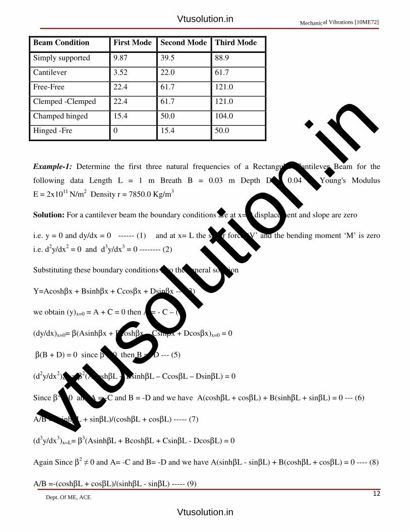
vtuso
lution
.in
12
Beam Condition First Mode Second Mode Third Mode
Simply supported 9.87 39.5 88.9
Cantilever 3.52 22.0 61.7
Free-Free 22.4 61.7 121.0
Clemped -Clemped 22.4 61.7 121.0
Champed hinged 15.4 50.0 104.0
Hinged -Fre 0 15.4 50.0
Example-1: Determine the first three natural frequencies of a Rectangular Cantilever Beam for the
following data Length L = 1 m Breath B = 0.03 m Depth D = 0.04 m Young's Modulus
E = 2x10¹¹
N/m2 Density r = 7850.0 Kg/m
3
Solution: For a cantilever beam the boundary conditions are at x= 0 displacement and slope are zero
i.e. y = 0 and dy/dx = 0 ------ (1) and at x= L the shear force ‘V’ and the bending moment ‘M’ is zero
i.e. d2y/dx
2 = 0 and d
3y/dx
3 = 0 -------- (2)
Substituting these boundary conditions into the general solution
Y=Acoshβx + Bsinhβx + Ccosβx + Dsinβx --- (3)
we obtain (y)x=0 = A + C = 0 then A = - C – (4)
(dy/dx)x=0= β(Asinhβx + Bcoshβx – Csinβx + Dcosβx)x=0 = 0
β(B + D) = 0 since β ≠ 0 then B = -D --- (5)
(d2y/dx
2)x=L= β
2(AcoshβL + BsinhβL – CcosβL – DsinβL) = 0
Since β2 ≠ 0 and A = -C and B = -D and we have A(coshβL + cosβL) + B(sinhβL + sinβL) = 0 --- (6)
A/B =-(sinhβL + sinβL)/(coshβL + cosβL) ----- (7)
(d3y/dx
3)x=L= β
3(AsinhβL + BcoshβL + CsinβL - DcosβL) = 0
Again Since β2 ≠ 0 and A= -C and B= -D and we have A(sinhβL - sinβL) + B(coshβL + cosβL) = 0 ---- (8)
A/B =-(coshβL + cosβL)/(sinhβL - sinβL) ----- (9)
Mechanical Vibrations [10ME72]
Dept. Of ME, ACE
Vtusolution.in
Vtusolution.in
vtuso
lution
.in
13
From equation (7) and (9) we have A(coshβL+cosβL) + B(sinhβL+sinβL) = 0 --- (10)
(sinhβL + sinβL) (coshβL + cosβL)
A/B = ---------------------- = ------------------------
(coshβL + cosβL) (sinhβL - sinβL)
Which reduces to coshβLcosβL + 1 = 0 ---------- (11)
Equation (11) is satisfied by a number of values of βL, corresponding to each normal mode of vibration,
which for the first three modes these values are tabulated in the table as
(β1l)2 = 3.52, (β2l)
2 = 22.00, (β3l)
2 = 61.70
Area A = 0.0012 m2 Moment of Inertia I = 1.600E-07m
4
Density per unit length (ρ*A) = ρL = 7850x 0.0012 = 9.4200 Kg/m
Circular Frequency
ωn1 = (β1l)2√(EI)/(ρl
4) = 2.052E+02 rad/sec
ωn2 = (β2l)2√(EI)/(ρl
4) = 1.282E+03 rad/sec
ωn3= (β3l)2√(EI)/(ρl
4) = 3.596E+03rad/sec
Natural Frequencies
fn1 = ωn1/2π = 32.639 Hz
fn2 = ωn2/2π = 203.994 Hz
fn3 = ωn3/2π = 572.111 Hz
Example-2: Determine the first three natural frequencies of a Rectangular Cantilever Beam for the
following data Length L = 1 m Breath B = 0.03 m Depth D = 0.04 m Young's Modulus E = 2.00E+11 N/m2
Density r = 7850.0 Kg/m3
Solution: For a cantilever beam the boundary conditions are at x= 0 displacement and slope are zero
Mechanical Vibrations [10ME72]
Dept. Of ME, ACE
Vtusolution.in
Vtusolution.in

vtuso
lution
.in
14
i.e. y = 0 and dy/dx = 0 ------ (1)
and at x= L the shear force ‘V’ and the bending moment ‘M’ is zero
i.e. d2y/dx
2 = 0 and d
3y/dx
3 = 0 -------- (2)
Substituting these boundary conditions into the general solution
Y=Acoshβx + Bsinhβx + Ccosβx + Dsinβx --- (3)
we obtain (y)x=0 = A + C = 0 then A = - C – (4)
(dy/dx)x=0= β(Asinhbx + Bcoshbx – Csinbx + Dcosbx)x=0 = 0
β(B + D) = 0 since β ≠ 0 then B = -D --- (5)
(d2y/dx
2)x=L= β
2(AcoshβL + BsinhβL – CcosβL – DsinβL) = 0
Since β2 ≠ 0 and A = -C and B = -D and we have
A(coshβL + cosβL) + B(sinhβL + sinβL) = 0 ---- (6)
A/B =-(sinhβL + sinβL)/(coshβL + cosβL) ----- (7)
(d3y/dx
3)x=L= β
3(AsinhβL + BcoshβL + CsinβL - DcosβL) = 0
Again Since β2 ≠ 0 and A = -C and B = -D and we have
A(sinhβL - sinβL) + B(coshβL + cosβL) = 0 ----- (8)
A/B =-(coshβL + cosβL)/(sinhβL - sinβL) ----- (9)
From equation (7) and (9) we have
A(coshβL+cosβL)+B(sinhβL+sinβL)= 0 --- (10)
(sinhβL + sinβL) (coshβL + cosβL)
A/B = ---------------------- = ------------------------
(coshβL + cosβL) (sinhβL - sinβL)
Which reduces to coshβLcosβL + 1 = 0 ---------- (11)
Mechanical Vibrations [10ME72]
Dept. Of ME, ACE
Vtusolution.in
Vtusolution.in

vtuso
lution
.in
15
Equation (11) is satisfied by a number of values of βL, corresponding to each normal mode of vibration,
which for the first three modes these values are tabulated in the table as
(β1l)2 = 3.52, (β2l)
2 = 22.00, (β3l)
2 = 61.70
Area A = 0.0012 m2 Moment of Inertia I = 1.600E-07m
4
Density per unit length (ρ*A) = ρL = 7850x 0.0012 = 9.4200 Kg/m
Circular Frequency
ωn1 = (β1l)2√(EI)/(ρl
4) = 2.052E+02 rad/sec
ωn2 = (β2l)2√(EI)/(ρl
4) = 1.282E+03 rad/sec
ωn3= (β3l)2√(EI)/(ρl
4) = 3.596E+03rad/sec
Natural Frequencies
fn1 = ωn1/2π = 32.639 Hz
fn2 = ωn2/2π = 203.994 Hz
fn3 = ωn3/2π = 572.111 Hz
Mechanical Vibrations [10ME72]
Dept. Of ME, ACE
Vtusolution.in
Vtusolution.in
![vtusolutionvtusolution.in/.../cse-viii-web_2.0___rich_internet_application_[06cs832]-notes.pdf · vtusolution.in Web 2.0 06CS832 Dept of CSE, 2 differences between HTML and Flex applications,](https://static.fdocuments.net/doc/165x107/5e058fb87f76f517fd59d4ac/vt-06cs832-notespdf-vtusolutionin-web-20-06cs832-dept-of-cse-2-differences.jpg)


![DATABASE MANAGEMENT SYSTEMS [10CS54] Notes - VTU Solutionvtusolution.in/uploads/9/9/9/3/99939970/cse-v-database_management... · DATABASE MANAGEMENT SYSTEMS . ... Classification of](https://static.fdocuments.net/doc/165x107/5ac2a75d7f8b9a4e7c8e8506/database-management-systems-10cs54-notes-vtu-management-systems-classification.jpg)


![INDUSTRIAL DRIVES & APPLICATIONS (06EE74)vtusolution.in/uploads/9/9/9/3/99939970/complete_[10ee74]-notes.pdf · INDUSTRIAL DRIVES & APPLICATIONS 10EE74 ... A First Course On Electric](https://static.fdocuments.net/doc/165x107/5aec939a7f8b9a585f8efaf5/industrial-drives-applications-06ee74-10ee74-notespdfindustrial-drives-applications.jpg)