Voter Uncertainty and Economic Conditions: A Lookinto Election Competitiveness

Christopher V. Lau∗

April 30, 2009

Abstract

It is widely know that the state of the economy has a substantial effect on howvoters vote. Unforunately, voter uncertainty during particular economic conditionsis often overlooked. In this study, I attempt to uncover how uncertain voters areduring an election by uncovering a relationship between election competitivenessand the state of the economy. Essentially, if an election is competitive, the outcomeis as good as random; overall, voters are uncertain of who they want to govern thestate. I use congressional elections from 1900 to 1976 to analyze these potentialeffects and find that the change in prices has the greatest effect on election compet-itiveness. Moreover, I find that, contrary to expectations, inflation actually makescandidates who are opposing an incumbent less competitive. Furthermore, I findthat unemployment has very little effect on election competitivness; this is in linewith the previous analysis of Gerald Kramer (1971) and George Stigler (1973). Inthe end, it is found that increases in the percent change of GNP lead to decreasesin electoral competition, as predicted. Also, increases in inflation cause electionswithout incumbents to become more competitive, while at the same time makingelections with third party incumbents less competitive. Elections where incumbentsare either Democrats or Republicans are left ambiguous.

∗I would like to thank Professor James Powell for his advice, guidance, and willingness to work withme on this Undergraduate Honors Thesis. I would also like to thank Eva Arceo-Gomez for helping mewith Stata.

1 Introduction

Over the past sixty years, economists and political scientists have tried to uncover the

properties of voting and elections. The goal of these studies is to develop and test theories

as to why voters vote for particular candidates; is it because of the candidates themselves

or the party they belong to? Or, is it because of some outside source? For example, David

Lee, Enrico Moretti, and Matthew Butler (2004) tried to shed light on a property of

voting by answering the question, “Do voters affect or elect policies?” Here, they wanted

to decipher between which voting theory was dominating, policy convergence or policy

divergence. In policy convergence, candidates moderate their platforms to address the

median candidate; they converge to the same platform in an attempt to gain as many

votes as possible. Obviously, this can only exist when the promises candidates make are

credible. Policy divergence drops the assumption that candidate promises are credible,

and concludes that voters vote for the candidate who shares the closest policy platform

to their own, since they know any promise by the candidate will be broken. Using close

elections as a quasi-experiment, Lee, Moretti, and Butler found that voters do not affect

policies, and instead elect them. Thus, the hypothesis that candidates alter their positions

with the hope of winning the election fails; the leading explanation presented was that

“the difficulty in establishing credible commitments to moderate policies” dominates any

possible effect of convergence.

A very common election hypothesis that is often tested is economic voting; the con-

cept that economic conditions affect election outcomes. While the acceptance of this

hypothesis has been well established, Richard Nadeau and Michael Lewis-Beck (2001)

attempted uncover another property: whether voters were retrospective or prospective.

That is, do voters cast their vote based on a candidate’s (or party’s) past economic

record, or on what they expect the economy to be in the future if a candidate is elected?

Using presidential elections from 1956 to 1996 , Nadeau and Lewis-Black found that

retrospective voting is used when a popularly elected president is running for reelection,

1

and prospective voting is used otherwise1.

Along similar lines, I too would like to uncover and test a property of elections.

Specifically, I would like to see whether or not economic conditions influence uncertainty

among voters. I begin my analysis with the assumption that a competitive election

implies, on average, that voters are unsure of who they would like to vote for, i.e. the

“representative voter” is uncertain of who they want to see in office. Thus, under this

assumption, I use election competitiveness as a proxy for how unsure voters are in a given

election. This assumption seems quite reasonable; Lee, Moretti and Butler essentially

used this assumption to form their quasi-experiment. They interpreted a close election

as an election with an outcome that is as good as random.

A large proprtion of the current literature has revealed that an incumbent loses votes

when their macroeconomic performance is poor. Ideally, I would like to answer the

question: do these losses in incumbent vote shares benefit a single competing candidate,

or benefit all other candidates in the election? Much of the current literature has assumed

the two party system (all other candidates outside of the two parties are not considered),

however examining almost any Congressional ballot clearly indicates voters usually have

more than two options. The problem with restricting analysis to two parties is that we

never get to see how other candidates are affected. When there are two candidates, an

incumbent losing votes clearly implies that the challenger will gain more, however if we

introduce more candidates, it is not clear that a single candidate will obtain the entire

incumbent residual. It could very well be the case that the incumbent’s residual votes

are retained by a third party candidate. It is even possible that the “primary” challenger

loses votes to third party candidates, thus leaving the effect of the economy on election

outcome lower than the “true value”. Thus, in this study, I would like to extend past

the typical two-party analysis, and see whether or not third party candidates earn more

votes during years of economic downturn.

1To test retrospective voting, change in the Nation Business Index (NBI) was used as a proxy. Totest prospective voting, change in the Economic Future Index (EFI) was used as a proxy.

2

I will proceed by sectioning this paper in the following way: Section 2 will deal with

a review of the past literature. I will summarize major economic voting theories and

findings, as well as address a study dealing with election competitiveness. Section 3

will present two models I would like to test. Section 4 discusses the data I used, and

estimation. Section 5 gives the results of my empirical analysis, and Section 6 concludes.

2 Literature Review

Before beginning our analysis of competitive elections, it will be useful to properly under-

stand a few economic voting theories, and the empirical test that support them. Gerald

Kramer (1971) developed an empirical model to test how economic conditions affect vot-

ing percentages of congressional candidates. Here, he made a crucial assumption for a

voter’s decision rule: voters only look at the performance of the incumbent. That is,

voters will vote for the incumbent if they deem his or her performance satisfactory. Oth-

erwise, the voter will allow the opposition a chance to govern. Kramer assumes that

voters completely ignore the qualities of all non-incumbent candidates and only focus

on those of the incumbent when making a decision. Under this assumption, Kramer

developes the following statistical model:

yt = V + λT + δt[α + β∆t] + ηt

where yt is party A’s share of the two-party vote, T allows for trends in partisanship, δt

is +1 if A is the incumbent and -1 if B is the incumbent, ∆t is a proxy for incumbent

performance, and ηt is a stochastic error term that consists of the net effects that affect

yt, not explained by the other covariates. In this model, V is considered the base vote for

party A, λ is the time trend coefficient, α is the incumbent’s advantage, and β reflects

the effect of the incumbent’s performance in office.

Kramer dealt with the error term, ηt, in two seperate ways. First he tested his model

3

under the assumption that ηt satisfies the Gauss-Markov assumptions by using Ordi-

nary Least Squares. Next, he assumed that during presidential elections, congressional

candidates obtained a “coattail” effect; that is, congressional candidates are effected by

the fact that they are a member of the same party as a presidental candidate. Since a

political party can be considered as a “team,” congressional candidates can be effected

by the campaign of the highly publicized presidental candidate. Thus, Kramer assumes:

ηt = ut + γvt

where ut is the disturbance from the congressional election, vt is the disturbance in the

presidental election, and γ (with 0 ≤ γ ≤ 1) is the effect of the presidential campaign on

the congressional vote. In Kramer’s analysis, he esitmated γ̂ using maximum likelihood

techniques, then preformed a weighted least squares with a weight that was a function of

γ̂. In addition, the proxies used in ∆t were (in percent change form) real income, prices,

and unemployment.

The results of his study found that all of the estimated equations explained a signifi-

cant amount of the vote; it was found that a likelihood ratio test of the hypothesis that

all coefficients except for the intercept and time trend term were zero was significant.

In addition, the models had R2 values between 0.48 and 0.64, indicating that all of the

equations explained a half to two-thirds of the variance in the vote. The coefficients

on the income terms in all of his equations were positive and significant, as expected

(increases in income increase an incumbent’s vote share), while the coefficients on price

were negative, with only a few significant. The coefficients on unemployment consis-

tently had the wrong sign (positive), however none were significantly different from zero.

Kramer explains this by a variety of factors, most notably, the possibility that those who

are typically unemployed at normal unemployment levels are also less politically active.

Suprisingly, all of the incumbency coefficients (α) were small and insignificant, indicating

4

that incumbency does not have an effect on vote share, contrary to intuition.

In the end, Kramer concluded that election outcomes are substantially responsive to

changes that occur under the incumbent party. Specifically, he found that a 10% decrease

in per capita real income would cost the incumbent party 4 to 5 percent of the vote share,

all else equal. Furthermore, Kramer concluded that real income was the most important

factor in determining election outcomes, and that incumbency itself was unimportant.

George Stigler (1973) attempted to further justify Kramer’s findings of an insignifi-

cant effect on unemployment, and improve his model. After replicating Stigler’s analysis

using the change in unemployment, relative change in per capita real income, and price

level, Stigler continues to find that there is not a significant relationship between vote

share and unemployment. His justification for this was that moderate changes in unem-

ployment would most likely affect a small proportion of the voting population. Stigler

also recognizes that multicollinearity may be a problem; the correlation between unem-

ployment and per capita real income is −0.78.

A few improvments and variations Stigler made on Kramer’s work included restoring

data from years the United States was in war (Kramer had dropped them), regressing over

two-year changes in economic activity, and demeaning the economic condition variables2.

With these modifications, it was found that both changes in real income and changes

in price both significantly affect the vote share between Democrats and Republicans

within an election. Stiger follows this analysis by questioning whether or not voters

directly evaluate economic conditions as a basis for voting; a decline in the economy is

not always due to poor governing by Congress. In addition, voters may not abandon an

incumbent because of a small hiccup; one does not sell stock in a corporation just because

it performed poorly on one day. Instead, Stigler argues that the voter judges which

candidate could maintain a high and steady rate of growth of income. To do this, voters

use past experiences to forecast how well a candidate (or party) will govern. Specifically,

2Stigler also tried to regress the change in vote share on the change in economic conditions. Thisregression resulted in a significant coefficient for income, and an insignificant coefficient for prices.

5

voters discount previous economic conditions by (1/(1 + r))t, where r is a discount rate.

In other words, past performance does influence how voters vote, yet not as strongly as

Kramer had assumed. Using discount rates of 0.10 and 0.25, Stigler found that there

is no significant relationship between vote share and average income performance. As a

result, “voters disregard average income experience in deciding between the parties.”

Ray Fair (1979) attempted to create a generalized model of the works by Kramer and

Stigler, which he followed by testing on Presidential elections. Instead of accepting either

of the theories assumed by Stigler or Kramer, Fair incorporated them in his model. He

first assumed a utility function for voter i’s expected future utility if either the Democratic

or Republican presidential candidate was elected at time t:

UDit = ξDi + βDM

Dt

URit = ξRi + βRM

Rt

where MDt and MR

t are vectors of preformance proxies for the last time a Democrat and

Republican were in office, respectively3. ξDi and ξRi are voter i’s respective utility for the

Democrat’s and Republican’s candidate, given economic performance. βD and βR are

vectors of coefficients.

It follows that voter i votes for the Democratic candidate when UDit > UR

it , i.e., we

can let Vit = 1{UDit > UR

it }. Rearranging, he defined

ψi = ξRi − ξDi

qt = βDMDt − βRMR

t

3To be exact, in Fair’s study, he lets

βDMDt = β1

Mtd1

(1 + ρ)t−td1+ β2

Mtd2

(1 + ρ)t−td2and βRM

Rt = β3

Mtr1

(1 + ρ)t−tr1+ β4

Mtr2

(1 + ρ)t−tr2

where tc1 is the last time party C was in office, tc2 is the second-to-last time party C was in office,Mtc1 is party C’s economic performance the last time party C was in office, Mtc2 is party C’s economicperformance the second-to-last time they were in office, and ρ is a discount rate

6

so that Vit = 1{qt > ψi}. Fair assumes that ψi has a uniform distribution between some

numbers a+δt and b+δt, where a and b are constant across all elections. Thus, ψ (where

the subscript is dropped due to aggregation) has a cumulitive distribution function of

F (ψ) =

0 for ψ < a+ δt;

ψ−a−δtb−a for a+ δt ≤ ψ ≤ b+ δt;

1 for ψ > b+ δt

It follows that the percent share of votes for the Democratic candidate is simply F (qt), i.e.

Vt = − ab−a + qt

b−a −δtb−a . He eventually simplifies this to a form α0 +α1qt + vt, where α0 =

− ab−a , α1 = 1

b−a , and vt = δtb−a . Inserting qt gives an estimatable equation. Furthermore,

after inspection of the residuals, vt, Fair finds that the problem of heteroskedasticity

exists; he solves this by using a general least squares procedure.

Fair applys his generalized model to presidential elections by specifying the measures

of economic performance to be the growth rate of GNP per capita, the absolute value of

the growth rate of prices, the level of unemployment and the change in unemployment,

over one, two, three and four years, giving him sixteen possible measures. He estimated

48 equations, with up to four regressors in each equation and found that the growth rate

of GNP per capita was the best measure of performance, with a coefficient of 0.0116.

This implies that a one percentage point increase in the growth rate of GNP per capita

is associated with a 1.16% increase in the incumbent party’s vote share. Unlike Kramer,

Fair found that the incumbent has an average advantage of about 3.5%. Furthremore,

he concludes that voters do not consider the past performance of the non-incumbent

party, and only consider the events that occured in the incumbent’s last term, which is

consistent with Kramer’s initial assumption.

Fair acknowledges that his findings are very limited; since he worked with only pres-

idential elections, he used 16 observations. Thus, we must take Fair’s empirical results

with a grain of salt.

7

The preceding studies have allowed us to examine the relationship between elections

and economic activity. We can now take a look at how electoral competitiveness has

previously been treated. Alan Abramowitz (1991) tried to explain why U.S. House in-

cumbents in the 1980’s were winning by larger margins compared to the 1950’s and

1960’s. He notes that the proportion of House incumbents to win over 60% of the vote

increased from 64% in the 1960’s to 78% in the 1980’s. Abramowitz tries to explain

this phenomenon by creating a model that explained competition; he regressed margin

of victory or defeat of the incumbent on a group of explanatory regressors4, and finds

that the most important determinant to the level of competition in House elections is the

challenger’s campaign spending. Interestingly, the coefficient on the incumbent’s amount

of spending was insignificant, indicating that the margin of victory is not influenced by

how much money the incumbent spends. Unfortunately, Abramowitz does not address

whether or not the condition of the economy has an effect on competition; there is no

clear direction to the causal relationship between competition and campaign spending.

Non-incumbent candidates may be spending more because of the fact that the election

is competitive; they already have a chance to win.

In addition, it is quite apparent that the state of the economy can affect how much

money a non-incumbent candidate gathers and spends. Unfortunately, either direction of

this relationship seems feasible. It could easily be the case that during a period of strong

economic performance, rival candidates are able to obtain more funding. Likewise, during

dismal economic times, contributors may be discouraged by the incumbent’s performance,

thus fund alternative candidates. In either situation, if my hypothesis is true, it could

be the case that economic conditions influence competition, which influences campaign

spending, in which case the economy is the true cause of competitiveness in U.S. House

elections.

4Regressors included partisanship of the district, incumbent’s personal popularity, incumbent’s se-niority, the type of committees the incumbent has served on, the incumbent’s rate of defection fromhis party, the incumbent’s campaign spending, the challenger’s campaign spending, the challenger’sexperience, and the party affiliation of the incumbent

8

3 Model

In this section, I will derive a basic model that can be used to estimate some election

properties of interest. What makes this model different than those used in previous

studies is two-fold. First, I will examine competitiveness, rather than outcome. Second,

I will explain this competitiveness using all nt candidates in each election, rather than

assuming third party candidates are negligible. One main advantage of this model is its

ability to disentagle incumbency effects in multi-candidate (greater than two) elections , a

concept that has rarely been studied in the previous literature. Specifically, I will present

two models, each with different assumptions regarding the use of “coattail” effects, i.e. the

effect of presidential incumbency on local elections. The second model is a generalization

of the first, with variations in the assumptions used to check the robustness of the original

specification, thus I will explain the first model in detail, and explain the other in less.

3.1 The baseline model

I will present my model in a similar derivation to that done by Ray Fair. First, we

assume that election t has nt candidates running for office. We can define Uict to be the

future expected utility of voter i in election t if candidate c wins. For voter i to vote

for candidate c, the future expected utility of voter i voting for candidate c will exceed

her expected future utility of voting for any of the other nt − 1 candidates in election t.

This is equivalent to saying the future expcted utility of voting for candidate c exceeds

the maximum utility gained from voting for any of the other nt − 1 candidates. Then,

we can let Pit(c) be a variable that indicates whether or not voter i voted for candidate

c in election t, i.e. the variable is equal to one if candidate c was voted for, and 0 if the

candidate was not. That is:

Pit(c) =

1 if Uict > maxk 6=c Uikt;

0 otherwise.

9

Then, let us define Xt to be a vector of covariates that describe the performance of the

economy during election t, Ict to be an indicator variable5 for whether or not candidate

c was an incumbent in election t, PTYct to be an indicator for whether or not candidate

c belongs to a major political party (Democrat or Republican) in election t, and PRSct

to be an indicator for whether or not candidate c is of the same party as the current

presidential administration in election t. Define the future expected utility of voter i

voting for candidate c in election t as:

Uict = Vct + εict (1)

Vct = γ + β1Ict +X ′tβ2 +X ′t · Ictβ3 + β4PTYct + PTYct ·X ′tβ5 + β6PRSct + ξct (2)

where γ is a constant and β1, β2, β3, β4, β5, and β6 are vectors of coefficients. Here, I

assume that political party status helps influence the effect of economic conditions on

competitiveness. Specifically, if candidate c belongs to a major political party, she should

be helped by a strong economy, and hurt by a weak one; candidates’ expected performance

is associated with their party. Since major party candidates are most often in power,

they take the greatest responsibility.

I define ξct as the stochastic error term from candidated c, which is the same across

all voters i who participate in election t, and εitc as the stochastic error term for voter

i when voting for candidate c in election t. If we assume that εitc is independently and

identically distributed according to an extreme value distribution, we can solve for the

probability that the representative voter, voter i, votes for candidate c as a multinomial

logit model:

Pt(c) =eVct∑ntj=1 e

Vjt, c = 1, ..., nt

That is, the percent voted for candidate c in election t is Pt(c).

To measure competitiveness of all candidates, I observe that the incumbent candidate

5In cases where indicator variables are multiplied by vectors, the variable is then either the identitymatrix, or the zero matrix

10

is typically considered as the most competitive. Thus, any judgement in competition

should be relative to the incumbent candidate, if one exists in the election. If we define

Pt(I) as the proportion voted for the incumbent candidate in election t, we can measure

competitiveness of candidate c in election t as Pt(c)/Pt(I). If an election is competitive,

this “competitiveness ratio” should be 1 for all candidates in election t. As a result, the

farther away the ratio is from 1, the less competitive the election.

However, not all elections have incumbents. This gives us a chance to measure in-

cumbency effects on competitiveness. For elections with incumbents, let Pt(1) = Pt(I).

In elections without incumbents, I let Pt(1) be defined as the proportion of votes gained

by the candidate whose last name is alphabetically first, Pt(A). If an election is competi-

tive, it should not matter who the other candidates are being compared against; the ratio

should be hypothetically 1 for all candidates, assuming alphabetic ordering of candidate

names is independent of qualifications and vote-getting ability. Thus, define INCt as an

indicator variable for whether or not there is an incumbent in election t, so that Pt(1)

can be defined as:

Pt(1) =

Pt(I) if INCt = 1;

Pt(A) if INCt = 0.

An implication of this definition is that candidate 1 is the incumbent when there exists

an incumbent in the election, and is the first alphabetical candidate when there does not

exist an incumbent. In addition, we define the competitiveness ratio for candidate c in

election t as Pt(c)/Pt(1). Notice that each election should have nt − 1 competitiveness

ratios, since comparing a candidate against herself will always yield a ratio of 1. In other

words, if we examine nt − 1 ratios, we can solve for the last, thus we are given complete

information regarding voting proportions in election t.

Let us assume that Pt(1) 6= 0. Then, using the multinomial logit model from the

11

utility function, an estimatable equation can be formulated:

Pt(c)

Pt(1)=

eVct/∑ntj=1 e

Vjt

eV1t/∑ntj=1 e

Vjt=eVct

eV1t

log[Pt(c)

Pt(1)] = log(

eVct

eV1t)

log[Pt(c)]− log[Pt(1)] = Vct − V1t

Using equation (2):

Vct − V1t = γ + β1Ict +X ′tβ2 +X ′t · Ictβ3 + β4PTYct + PTYct ·X ′tβ5 + β6PRSct + ξct

−(γ + β1I1t +X ′tβ2 +X ′t · I1tβ3 + β4PTY1t + PTY1t ·X ′tβ5 + β6PRS1t + ξ1t)

= −β1(I1t)−X ′t · I1tβ3 + β4(PTYct − PTY1t) +X ′tβ5(PTYct − PTY1t) +

β6(PRSct − PRS1t) + (ξct − ξ1t)

Since candidate 1 is defined as the incumbent if there exists one, and the first alphabetical

candidate when there is not, we can observe that I1t = INCt, i.e. if there is an incumbent

in the election, then candidate 1 is the incumbent. Furthermore, PTYct−PTY1t can take

on three values: 1 if candidate c is in a major political party and candidate 1 is not, 0

if both candidates are not in a major political party or both candidates are in a major

political party, and −1 if candidate c is not in a major political party and candidate 1 is

in a major political party. Therefore, we can define:

Pct =

1 if candidate c is in a major political party and candidate 1 is not;

−1 if candidate c is not in a major political party and candidate 1 is;

0 otherwise.

Similarly, PRSct−PRS1t can take on three values: 1 if candidate c belongs to the party

of the current president, 0 if neither or both candidates belongs to party of the current

president, and −1 if candidate 1 belongs to the party of the current president. We then

12

define:

CTct =

1 if candidate c belongs to the party of the president;

−1 if candidate 1 belongs to the party of the president;

0 otherwise.

This will allow us to measure “coattail” effects. Therefore, if we let ηct = ξct − ξ1t, we

can simplify:

log[Pt(c)]− log[Pt(1)] = α0INCt + INCt ·X ′tα1 + α2Pct + Pct ·X ′tα3 + α4CTct + ηct (3)

where α0 = −β1, α1 = −β3, α2 = β4, α3 = β5, and α4 = β6. The term ηct represents the

net effect of factors not explicitly considered in the model above.

It should be noted that if there is no incumbent in the election, if the two candidates

being compared are either both apart of a major political party, or are both not, and

if neither or both candidates belong to the President’s party, then the competitiveness

ratio will depend completely on the stochastic error term. This is quite intuitive: If

there is no incumbent and both candidates are from “unknown” political parties, the

candidate to win more votes should win by a very slight margin and should be essentially

random. Similarly, if there is no incumbent and both candidates are from major political

parties, the candidate who wins more votes should depend on other factors not explicitly

explained in the model; usually unobservable (rather, unmeasureable) characteristics.

That is, in an election where no one is already well known (not the incumbent), then

voting decisions should depend on party affiliations. If the effect of each candidate’s party

affiliation cancels out, i.e. the two candidates both belong to major political parties, or

both belong to minor political parties, then the election should be relatively close and

random. In these types of elections, economic performance is not considered because

either both candidates belong to minor political parties, in which case they take no

responsibility for the economy, or they both belong to a major political party, where the

effect cancels out.

13

I now examine the error term, ηct, further. Two other factors that could influence the

closeness of an election is trends in time and the number of candidates in the election.

Let T represent time trend; it takes the value 1 for the first year an election is held in

the sample, and N for the N th year after. For example, in the sample used in the next

section, we start from elections taking place in 1900. Thus, elections in this year will

have T = 1. In 1902, T = 2, and in 1970, T = 36. In addition, we would also like to

analyze how elections with incumbents are affected over time. To do this, we include the

interaction between incumbent in election status and time, i.e. INCt · T .

Furthermore, let Ct be a vector of indicator variables for the number of candidates in

election t. Precisely, if C1t = 1{∃ 1 candidate in election t},...,C11t = 1{∃ 11 candidates

in election t}, then:

C ′t =[C1t C2t ... C10t C11t

]

It follows that we can decompose ηct into the following:

ηtc = α5T + α6INCt · T + C ′α7 + vct

where α5, α6 and α7 are vectors of coefficients, and vct is interpreted as the net effect

of factors not explicitly considered by the model. Replacing this decomposition into

equation (3) gives:

log[Pt(c)]−log[Pt(1)] = α0INCt+INCt·X ′tα1+α2Pct+Pct·X ′tα3+α4CTct+α5T+α6INCt·T+C ′α7+vct

(4)

If it is assumed that vct ∼ N(0, σ2), then an ordinarly least squares regression can be

used to estimate the coefficients.

Each coefficient can be used to assess a property of elections. α0 measures the effect

of having an incumbent in an election on competitiveness, α1 measures how economic

performance affects competitivness when an incumbent is in the election, α2 measures the

effect of being in a major political party, α3 measures how economic performance affects

14

competitiveness when a candidate is a member of a major political party, α4 measures

the effect of competitiveness on being in the same political party as the president, α5

measures time trend effects when there is no incumbent in the election, α6 measures time

trend coefficients when there exists an incumbent in the election and α7 measures the

effect of the number of candidates in an election.

In general, we expect to see α0 < 0, i.e. on average, having an incumbent in the

election makes all other candidates less competitive. Furthermore, α2 should be greater

than zero; if candidate c is a member of a major political party and candidate 1 is not, we

expect candidate c to be more competitive relative to candidate 1. Since being a member

of the presidential political party should help a candidate, we expect to see α4 > 0.

The sign of the time trend coefficient α5 is ambiguous; evaluating how competitiveness

changes over time when there is no incumbent in the election can be reasoned to be

both positive and negative. However, we might expect it to be close to zero. Finally,

according to Abramowitz (1991), House elections with incumbent candidates have become

less competitive over time, thus we hope to find α6 < 0, i.e. incumbents win by greater

amounts in later years.

When looking at the economic performance proxies, we would expect to see the co-

efficient on the interaction between party status and GNP to be positive; if candidate

c is in a major party and candidate 1 is not, then an increase in GNP should help the

candidate who is in a major party. The coefficient on the interaction between party

status and prices, and between party status and unemployment, should be negative;

increases in these variables indicate that there has been poor economic performance,

thus elections should become more competitive for those not in a major political party.

The coefficients on the interaction between incumbent in election status and economic

performance variables should be as follows: the interaction with GNP should be nega-

tive, while the interaction with prices and unemployment should be positive. That is,

poor economic performance should should lead to increased competition for alternative

15

candidates against the incumbent.

3.2 Non-incumbent coattail effects

In this second model, I try explain coattail effects in a different manner. In the previous

model, I measured coattail effects within the individual’s utility function through the use

of the indicator variable PRSct. However, it is very well possible that individual voters

do not give an extra benefit to the incumbent for being apart of the president’s party. In

this case, I redefine equation (1) as:

Uitc = γ+β1Ict+X ′tβ2 +X ′t · Ictβ3 +β4PTYct+PTYct ·X ′tβ5 +β6PRSct(1− Ict)+ εitc (5)

That is, a candidate is affected by the presidential party only if they are not the incum-

bent. Through similar derivations of model 1, if we let:

CTEct =

PRSct if I1t = 1

Ect if I1t = 0

It follows that the equation to be estimated becomes:

log[Pt(c)]−log[Pt(1)] = α0INCt+INCt·X ′tα1+α2Pct+Pct·X ′tα3+α4CTEct+α5T+α6INCt·T+C ′α7+vct

(6)

Again, if vct ∼ N(0, σ2), we can use OLS procedures to estimate the coefficients. In

addition, all coefficients should have the same interpretation as before.

4 Data and Estimation

To estimate the relationship between economic conditions and competition, I use results

from congressional elections. There are two main reasons I chose this dataset. The first

reason is that there is a very large number of observations; since congressional elections

16

are held for every district, in every state, every two years, we can bypass some of the

problems of limited observations found in previous studies, such as that acknowledged

by Fair (1979). The second reason is that non-major party candidates can be more

influential in congressional elections. That is, third party candidates need less resources

to be competitive and are less likely to be at a disadvantage because of well known major

party candidates.

Data for congressional elections was collected from the Inter-University Consortium

for Political and Social Research. In this data set, I received the following information

for each candidate: identification codes, the year of election, party of the candidate, the

number of votes cast for the candidate, the total number of votes cast in the election, the

number of candidates in the election, a dummy variable for incumbency, and a dummy

variable for outcome. From this information, I was able to form the dependent variable,

log(Pt(i)/Pt(1)),∀t,∀i 6= 1.

To obtain data on economic performance, I chose to use data on national economic

indicators. This choice was made over state or district data because Congress typically

affects national policies, rather than local, thus they should be judged at the national

level. Precisely, I used the economic data provided in Fair’s (1979) article in the Review

of Economics and Statistics. In the appendix, I present Table A, where the data for

performance proxies are displayed: percent change in real per capita GNP (in 1972

dollars) over one and two years, percent change in unemployment rates over one and two

years, and percent change in GNP deflator (with 1972 = 100.0) over one and two years.

The years covered in this study are from 1900 to 1976; after ensuring that each election

has nt− 1 observed candidates, where nt is the number of candidates in election t, I end

up with 29,967 observations.6

In Table 1 I present a decomposition of the percent voted statistic, Pt(c). It can be

found that on average, the incumbent wins 62.3% of the vote when they are in an election;

6We have only nt − 1 candidates per election, since one candidate is used as the denominator of thecompetitiveness ratio.

17

this clearly indicates that my assumption of an incumbent’s superior competitiveness is

correct. Furthermore, of non-incumbents, those who are members of major parties win

39.5% of the vote on average, and those who are not members of major parties only win

3.9% of the vote.

Table 1: Summary of Percent Vote by Incumbent and Party Status

Incumbents Non-Incumbents in Major Party Non-Incumbents not in Major Party

Mean S.D. Mean S.D. Mean S.D.

Percent voted for in election 0.623 0.143 0.395 .146 0.0391 0.0820

In Table 2, I present statistics to summarize some of the important covariates. Upon

inspection, over two-thirds of congressional elections from 1900 to 1976 had three or

more candidates, indicating that the typical assumption of two candidates is weak. The

fact that a large proportion of elections involve more than two candidates is the primary

reason why this paper examines all candidates in a given election; two party models do

not fully explain most elections. In addition, 84.9% of elections contained an incumbent

and 61.9% of the candidates were members of a major political party. About half of

those who were members of a major political party were members of the same party as

the President.

Table 2: Summary of Covariates

Percentage S.D. Percentage S.D.

C2 0.325932 0.468727 C9 0.001182 0.034353

C3 0.276444 0.447244 C10 0.000468 0.021632

C4 0.235092 0.424061 C11 0.000245 0.015658

C5 0.107715 0.310024 PRS 0.310573 0.462733

C6 0.035578 0.185238 INC 0.848741 .3583132

C7 0.012305 0.110246 I 0.279587 0.448801

C8 0.005038 0.070801 PTY 0.618917 0.485658

CN = Percent of elections with N candidates

PRS = Percent of candidates in same party as President

INC = Percent of elections with an incumbent

I = Percent of candidates who are incumbents

PTY = Percent of candidates in a major party

18

4.1 The baseline model

We can now proceed to estimate the coefficients of interest. If we assume E(vct) = 0,

then the following OLS estimates of equation (4), presented in Table 3, will be correct.

As a base case for interpretation, Table 3 presents equations that include the economic

condition variables growth in GNP and change in inflation7. Precisely, if we let G1t and

G2t be the growth rate of GNP over 1 and 2 years at election t, respectively, and Pr1t

and Pr2t be the change in inflation over 1 and 2 years at election t, respectively, then:

X ′t =[G1t Pr1t

]for equation 4.1.1

X ′t =[G2t Pr2t

]for equation 4.2.1

The only difference, then, between equations 4.1.1 and 4.2.1 is the lag structure of the

desired economic variables. Equation 4.1.1 contains economic variables that are lagged

one year. That is, for the year 1970, if we let GNP (X) be the annual GNP for year X,

G11970 is given by:

G11970 =GNP (1970)−GNP (1969)

GNP (1969)

We can find the change in price level in a similar manner. Equation 4.2.1 containts eco-

nomic variables that are lagged two years, i.e. for the year 1970, we replace GNP (1969)

with GNP (1968) to obtain G21970.

7Growth and inflation were used because unemployment has been previously shown to be an inaccu-rate measure for economic conditions, and this regression explained the most variability in the data.

19

Table 3: Regression Output for Equation (4)

4.1.1 4.2.1

Coef. S.E. t P > |t| Coef. S.E. t P > |t|

INC -1.46584 0.031155 -47.05 0 -1.49354 0.031303 -47.71 0

INC ·G -0.49058 0.23245 -2.11 0.035 0.174485 0.169531 1.03 0.303

INC · Pr -1.51518 0.30675 -4.94 0 -0.60523 0.166943 -3.63 0

P 4.182622 0.032108 130.27 0 4.086285 0.031953 127.88 0

P ·G 0.850794 0.370161 2.3 0.022 1.485549 0.271976 5.46 0

P · Pr -3.13866 0.475446 -6.6 0 -0.93914 0.246123 -3.82 0

CT 0.109576 0.044544 2.46 0.014 0.106718 0.044623 2.39 0.017

T 0.005501 0.001084 5.08 0 0.005426 0.001084 5 0

INC · T -0.24235 0.046803 -5.18 0 -0.23826 0.046881 -5.08 0

Adj −R2 0.7041 0.704

Note: Standard errors are robust; 4.X.1 uses economic changes over X year(s)

Equation 4.1.1 shows that all of the coefficients are significantly different from zero

at the 5% level. In equation 4.2.1, the only coefficient that is not significantly different

from zero at the 5% level (nor the 10% level) is the interaction between incumbency

and growth in GNP. Note that all coefficients that do not involve an economic condition

variable are similar in both equations, as we would expect. In addition, they are of

the same sign as we had predicted earlier; the non-incumbent time trend coefficient is

slightly, yet significantly, positive. The coefficients of terms that do involve economic

conditions variables, however, are very different in the two equations. A change in price

over one year has a larger effect in absolute value on candidates who are in an election

with an incumbent and/or are members of a major party than over two years, yet growth

in GNP over two years affects major party candidates more than growth over one year.

Finally, all significant coeffficients on terms that involve economic conditions variables

hold the correct sign except for the interaction between prices and incumbency. This

can possibly be explained by the fact that voters directly observe nominal wages, and

not real. Increases in the price levels will usually lead to increases in nominal income.

This increase may give voters the perception that their congressional representative’s

performance is satisfactory, and thus will reelect the incumbent.

20

In Table B of the appendix, I present variants of the above two equations that I also

tested. For X ∈ {1, 2}, 4.X.2 includes only growth in GNP, 4.X.3 includes only changes

in prices, 4.X.4 includes only changes in unemployment, and 4.X.5 includes changes in

prices and unemployment.

4.2 Non-incumbent “coattail” effects

The second model adds the assumption that incumbents do not gain from being a mem-

ber of the current president’s party, yet non-incumbents find this quality beneficial. To

support this assumption, Table 4 presents the average percent vote of candidates by

presidential party status and incumbency. It can easily be seen that, on average, incum-

bents who are not a member of the President’s party earn a slightly higher percent of

the vote than incumbents who are members of the President’s party. Furthermore, of

non-incumbents, those who are a member of the President’s party earned a much larger

proportion of the votes compared to those who were not members of the President’s

party. It is quite clear that incumbents gain no advantage from having the same political

affiliation as the President, unlike non-incumbents, therefore justifying the use of the

second model.

Table 4: Percent vote by Presidential party status and incumbency

Incumbent Non-incumbent

Member of President’s party 0.608464 0.493548

Not a member of President’s party 0.639486 0.252267

Again, for interpretation, I use growth in GNP and change in inflation to measure

the effect of economic conditions on congressional election competitiveness. In Table 5,

equation 6.1.1 presents the regression output using changes in economic variables over

one year, while equation 6.2.1 presents the regression output using changes in economic

variables over two years.

21

Table 5: Regression Output for Equation (6)

6.1.1 6.2.1

Coef. S.E. t P > |t| Coef. S.E. t P > |t|

INC -1.78038 0.03924 -45.37 0 -1.80274 0.03918 -46.01 0

INC ·G -0.40881 0.224286 -1.82 0.068 0.157099 0.163701 0.96 0.337

INC · Pr -1.46412 0.29524 -4.96 0 -0.5856 0.160205 -3.66 0

P 4.005888 0.033395 119.95 0 3.910756 0.033219 117.73 0

P ·G 0.97041 0.363731 2.67 0.008 1.528109 0.267442 5.71 0

P · Pr -3.48784 0.467465 -7.46 0 -0.5856 0.160205 -3.66 0

CTE 0.693637 0.043776 15.85 0 0.68799 0.043848 15.69 0

T 0.005202 0.001087 4.79 0 0.005097 0.001087 4.69 0

INC · T -0.39607 0.024758 -16 0 -0.39275 0.024805 -15.83 0

Adj −R2 0.7067 0.7065

Note: Standard Errors are robust, 6.X.1 uses economic changes over X year(s)

As expected, the relationship between using one and two year changes of economic

condition variables is the same as that presented by Table 3: changes in competition

for major party candidates and candidates facing an incumbent are most drastic when

examining prices over one year. Likewise, growth seems to have very little effect on

competition when there is an incumbent, however helps a major party candidate the

most when it is examined over two years. It should be noted that the coefficient on

the interaction between incumbency and growth of GNP changes from significant at 5%

significance in equation 4.1.1, to insignificant at 5% significance in equation 6.1.1, which

implies that after controlling for the fact that incumbents do not recieve any beneficial

“coattail” effect, growth in GNP does not significantly affect the competitiveness of an

election involving an incumbent.

Comparing Table 3 and Table 5 shows that including non-incumbent “coattail” ef-

fects result in an increase in the absolute effect of having an incumbent in the election.

In addition, the effect of being a major party candidate is slightly smaller, while the

“coattail” effects and the incumbency time trend effect are both larger in absolute value.

The coefficients on the interaction between incumbent in election status and both of

the economic condition variables decreased in absolute value, and the coefficients on the

interaction between major party status and the economic condition variables increased.

22

This implies that including non-incumbent coattail effects causes major political party

status to be more responsive to changes in the economy, relative to before the effects

were included, while incumbent in election status becomes less responsive.

Similar to the baseline mode, I used different combinations of economic condition

variables in variant regressions, but felt that those presented in Table 5 fit the relationship

between competitiveness and the economy the best. In the appendix, I use Table C to

present the other regressions used.

5 Results

5.1 Evaluation of findings

After finding estimates for both the baseline model and non-incumbent coattail effect

model, it seems that economic conditions do have an effect on competitiveness of con-

gressional elections. To ensure this is true, I test whether or not the coefficients on all

variables that include an economic condition variable are not influential in the equation

and are identically zero, i.e. if we let δXY be the coefficient on the interaction between

X and Y , where X ∈ {INCt, Pct} and Y ∈ {G1t, G2t, P r1t, P r2t}, then we test the

null hypotheses at α = 0.05, H0 : δINCtG1t = δINCtPr1t = δPctG1t = δPctPr1t = 0, and

H0 : δINCtG2t = δINCtPr2t = δPctG2t = δPctPr2t = 0, for both equations (4) and (6). Table

6 presents the results of these hypothesis tests:

Table 6: F-tests for relationship of joint relationships

Equation 4.1.1 4.2.1 6.1.1 6.2.1

F-statistic 15.81 12.68 17.86 14.07

P > F 0 0 0 0

Note: df = (4, 29947)

Thus, we can reject the null hypothesis that economic conditions are not related

to competitiveness in all four equations at α = 0.05. We still do not know anything

about how particular economic changes related to competitiveness; since changes in each

23

particular economic variable are broken up between incument in election and major party

statuses, we cannot see the total effect of how an increase in inflation, for example, affects

the competitiveness of a particular candidate. To analyze this, we must recognize that

there are six kinds of candidates:

1. In an election with an incumbent and apart of a major political party, while the“base” candidate8 is not.

2. In an election with an incumbent and not apart of a major party, while the “base”candidate is.

3. In an election with an incumbent with both candidates either apart of a majorpolitical party, or not.

4. Not in an election with an incumbent and a member of a major party, while the“base” candidate is not.

5. Not in an election with an incumbent and not a member of a major party, whilethe “base” candidate is.

6. Not in an election with an incumbent with both candidates either apart of a majorpolitical party, or not.

The effect of economic conditions on the competitiveness of candidates type six is

zero, by assumption. The effect of economic conditions for candidates type four is the

coefficient of the interaction between major party status and the economic variable of

interest. The effect of candidates type five is the coefficient of the interaction between

major party status and the economic variable of interest multiplied by −1. The coefficient

on the interaction between incumbent in election status and the economic variable of

interest is the effect of the economy on competitiveness for candidates type three. The

sum of the coefficients on both interaction terms that involve the economic variable of

interest is the effect on the competitiveness of candidates type one, while the difference

is the effect on candidates type two.

We expect competitiveness of candidates type two, type three, and type five to have

a positive relationship with inflation, competitiveness of candidates type four to have a

8By “base” candidate, I am referring to candidate 1

24

negative relationship with inflation, and competitiveness of candidates type six to have

no relationship with inflation9. As noted earlier, the coefficient on incumbent in election

status and inflation (essentially, candidate type three) was of the wrong expected sign

(negative), however I already supplied a possible reason for this (voters observe nominal

wages). In addition, the relationship between inflation and competitiveness is ambiguous

for candidate type one; an increase in inflation should cause an increase in competitiveness

for some candidate c since an incumbent is in the election, however it should also cause

a decrease in competitiveness since candidate c is of a major party. This relationship,

because of the ambiguity, is of particular interest to test.

The relationships represented by candidates type three through six have been tested

in the previous section when evaluating whether or not the coefficients were significantly

different from zero10. Then we can run an F-test for the following null hypotheses, at

α = 0.05:

1. H0 : δINCtP1 + δPctP1 = 0, in favor of the alternative HA : δINCtP1 + δPctP1 < 0.

2. H0 : δINCtP2 + δPctP2 = 0, in favor of the alternative HA : δINCtP2 + δPctP2 < 0.

3. H0 : δINCtP1 − δPctP1 = 0, in favor of the alternative HA : δINCtP1 − δPctP1 > 0.

4. H0 : δINCtP2 − δPctP2 = 0, in favor of the alternative HA : δINCtP2 − δPctP2 > 0.

The results of the four hypothesis tests are presented below in Table 7. Seeing that

δINCtP1, δPctP1, δINCtP2, and δPctP2 are all significantly negative, it is sensible to test

whether or not candidates type one are less competitive when inflation increases, i.e. it

is beneficial to be an incumbent from a non-major party against an opponent from a

major party during times of increasing inflation. Here, we only test the hypotheses for

equation (6). Corresponding hypotheses are tested for equation (4) in Table D of the

appendix.

9Since an increase in inflation should represent the same economic condition as a decrease in thegrowth of GDP, we expect the relationship between growth and competitiveness to be opposite in signas the relationship between inflation and competitiveness.

10All coefficients involving inflation were significant, while the interaction between growth in GNPand incumbency were insignificant for equations 4.2.1, 6.1.1, 6.2.1. The coefficient on the interactionbetween prices and incumbency was of the wrong expected sign, however was significantly negative.

25

Table 7: One-sided F-tests for sign of inflation relationship in equation (6)

Hypothesis 1 2 3 4

F-statistic 53.88 17.56 26.21 7.32

P > F 1.092× 10−13 23.35× 10−7 1.54× 10−7 0.0034

Note: df = (1, 29947)

At α = 0.05, we can reject the four null hypotheses. Thus, the competitiveness of

candidates type one are negatively related to inflation; the benefits the incumbent from a

non-major political party gains outweighs the losses from increased inflation when facing

a major party opponent. However, it should be noted that in general, the benefit of being

an incumbent outweighs the losses from inflation, contrary to our original expectations.

In addition, the competitiveness of candidates type two are positively related to inflation,

as we had hoped; third party candidates become more competitive against the incumbent

when inflation increases.

Similarly, I can analyze the potential relationships for candidates type one and two

when using the growth in GNP instead of inflation. The null hypotheses at α = 0.05 are:

5. H0 : δINCtG1 + δPctG1 = 0, in favor of the alternative HA : δINCtG1 + δPctG1 > 0.

6. H0 : δINCtG2 + δPctG2 = 0, in favor of the alternative HA : δINCtG2 + δPctG2 > 0.

7. H0 : δINCtG1 − δPctG1 = 0, in favor of the alternative HA : δINCtG1 − δPctG1 < 0.

8. H0 : δINCtG2 − δPctG2 = 0, in favor of the alternative HA : δINCtG2 − δPctG2 < 0.

Table 8 gives the output of the four hypothesis tests using equation (6). I also tested

the hypotheses using equation (4); these are presented in Table D of the appendix.

Table 7: One-sided F-tests for sign of growth relationship for (6)

Hypothesis 5 6 7 8

F-statistic 1.15 19.17 20.91 38.78

P > F 0.14177 6.01× 10−6 2.42× 10−6 2.408× 10−10

Note: df = (1, 29947)

For hypothesis five, we fail to reject the null hypothesis that the effect of growth

in GNP over one year on competitiveness is zero for candidate type one; there is no

relationship between changes in GNP over one year and competitiveness of elections

26

for major party candidates competing against non-major party incumbents. There is,

however, a positive relationship when voters examine growth in GNP over two years. The

negative relationships confirmed in hypotheses seven and eight are as expected; increases

in GNP hurt third-party candidates in elections that contain incumbents. To summarize

the types of candidates and the change in their competitiveness as a response to the

economy, Table 8 is presented below for changes in inflation, and Table 9 for changes in

growth.

So far, I have ignored the potential relationship between competitiveness and unem-

ployment. This is because, similar to what Kramer and Stigler have found, the rela-

tionship between unemployment and elections, specifically competitiveness, is essentially

insignificant. Like Stigler, I argue that this finding is intuitive. Unemployment is not

only the result of a poor economy, but also of poor performance by workers, who are

potential voters. Corporations often fire those who they can afford to dispose of: those

who are young and unqualified, and those who are inadequate and unmotivated. If these

are the types of people who are less likely to vote, then their “displeasure” of being laid

off will not be voiced in an election, thus there would be no relationship between unem-

ployment and election competitiveness. That is, those who actually do vote will vote as

if unemployment was not a problem (since it is not for them!). Therefore, inflation and

growth in GNP should be more appropriate factors to consider.

When debating which economic variable, inflation or growth, affects election com-

petitiveness more, the previous analysis concludes that inflation is a more important

factor. This result is quite inuitive: prices are completely observable by voters. Voters

can respond to changes in prices because they often see them change first hand; every-

day, voters buy products for business and pleasure. They know when prices and wages

increase, and can make voting decision regarding them easily. The growth in GNP is not

as easily observable; it is not apparent to everybody in the voting population that there

has been a mild decrease in the rate that GNP increases. Not everybody readily knows

27

or observes this fact. As a result, voters make voting decisions primarily from observable

factors, such as prices; in turn, these voting decisions will either increase or decrease the

competitiveness of an election.

5.2 Election competitiveness and voter uncertainty

We return back to the original question of this paper: how does voter uncertainty change

with economic conditions? We initially assumed that voters are more uncertain when

elections are more competitive. However, the previous analysis has focused on how the

competitiveness of individual candidates respond to the economy; we can now evaluate

how overall election competitiveness changes. For an election to be more competitive,

we expect to see those who typically obtain the most votes to have a decrease in their

competitiveness ratio, and those who typically obtain the least votes to have an increase

in their ratio. That is, when facing an incumbent, major party candidates should have an

increase or no change in the competitiveness ratio, while third party candidates should

have an increase in the competitiveness ratio. When not facing an incumbent, major

party candidates should have a decrease in their competitiveness ratio, while third party

candidates should still have an increase.

Table 8: Summary of changes in competitiveness of candidate c caused by changes in inflation

Candidate c

Major Party Third Party

Incumbent/Major Party ↓ ↑

1 Incumbent/Third Party ↓ ↓

Non-incumbent/Major Party − ↑

Non-incumbent/Third Party ↓ −

Note: All relationships are determined from F-tests from Section 5.1

Type X : Candidate c; Candidate 1

Type 1: Major; Incumbent/Third

Type 2: Third; Incumbent/Major

Type 3: Third; Incumbent/Third and Major; Incumbent/Major

Type 4: Major; Non-incumbent/Third

Type 5: Third; Non-incumbent/Major

Type 6: Third/Non-incmbent/Third and Major; Non-incumbent/Major

28

From examining Table 8, we can decipher how the competitiveness of each type of

candidate reacts to changes in inflation; this will allow us to interpret the reaction in

overall election competitiveness. In Table 8, the rows are essentially the types of elections,

while the columns are the types of candidates in these elections. That is, the rows give

qualities of candidate 1, the columns give qualities of candidate c, and the relationships

(the arrows) in the table represent changes in the competitiveness ratio for increases in

inflation11. For example, in an election without an incumbent and where the “base”

candidate belongs to a third party, a major party candidate c is predicted to become

less competitive relative to the “base” candidate when there are increases in inflation.

This situation corresponds to the last row, first colomn in Table 8. Furthermore, we

can interpret the relationship between changes in inflation and election competitiveness

by ensuring that there are no conflicting relationships across election type (the rows).

It should be noted that − is interpreted as neutral, so if, for example there are three

candidates, and one candidate has no change (−) in competition relative to the “base”

candidate and another has an increase (↑) in competition relative to the “base” candidate,

then electoral competition has increased overall. If there are conflicting relationships,

i.e. one type of candidate increases competition (↑), while another decreases (↓), the

interpretation is left ambiguous.

It is easy to tell that in elections without incumbents, candidates who are members

of non-major parties benefit the most from increases in inflation12, while major party

candidates either have a decrease in competitiveness, or no change. Thus, we can conclude

that elections with no incumbents become more competitive as the change in inflation

increases. The cases when there exists an incumbent in the election is a little more

difficult to interpret. When the incumbent is a third party candidate, we can determine

11To be clear, ↑ indicates an increase in the competitiveness ratio, ↓ indicates a decrease in thecompetitiveness ratio, and − indicates no change

12In the bottom row of Table 8, the decrease in a major candidate’s competitiveness is actually anincrease in the third party candidate’s competitiveness, since the “base” candidate is a non-incumbentfrom a third party.

29

that the advantage of being a third party candidate outweighs any possible disadvantage

of being an incumbent when inflation increases, which makes elections less competitive.

We should note that these elections are very rare; elections that contain non-major

party incumbents have only occured in 3.36% of all congressional elections between 1900

and 1976. When the incumbent is of a major party, an opponent from another major

party actually loses votes, while third party candidates gain votes. Therefore, if there

are enough quality third party candidates, elections can become more competitive when

inflation increases, however the relationship is not well defined in general.

We can also examine how competitiveness responds to changes in GNP. Table 9

presents information similar to that found in Table 8. Clearly, in all election cases, when

GNP increases, competition decreases or does not change; that is, third parties gain less

of the vote share in all cases they are not the incumbent (with corresponding increases

for major party candidates) and there is no change when the incumbent is a third party

candidate. This is consistent with the hypothesis that an increase in GNP will cause a

decrease in electoral competition.

Table 9: Summary of changes in competitiveness of candidate c caused by changes in GNP

Candidate c

Major Party Third Party

Incumbent/Major Party − ↓

1 Incumbent/Third Party − −

Non-Incumbent/Major Party − ↓

Non-Incumbent/Third Party ↑ −

Note: All relationships insignificantly different from zero were considered as no change (−).

5.3 Problems and possible improvements

Throught this paper, I have tried to minimize the number of errors made. However, a few

potential problems do arise; I would like to address them in this section. One potential

criticism is the use of Table 4 to justify non-incumbent coattail effects. The problem

arises because of the fact that the President always belongs to a major political party.

Thus, since major party candidates tend to earn higher percentages of the vote share in

30

general, the disparity found for non-incumbents may just reflect the fact that candidates

in third parties earn such a small portion of the vote. In Table 10, I present the percent

vote of non-incumbents broken down by Presidential and major party status. It is found

that non-incumbents who are major party candidates actually do earn more if they are

not a member of the President’s party. Note that since there has never been a third

party candidate as president, there are no observations for candidates who are not from

a major party and of the same party as the President.

Table 10: Percent vote of non-incumbents by Presidential and candidate party status

Non-incumbent (Major party) Non-incumbent(Non-major party)

Member of President’s party 0.388908 -

Not a member of President’s party 0.401123 0.039111

By observation, it seems that being apart of a major political party will negate the

potential of coattail effects. This can be seen through Table 11; candidates who are

members of the President’s political party earn just as much as as candidates who are

member’s of the other major political party.

Table 11: Percent vote by Presidential and candidate party status

Member of Major Party Not a member of major party

Member of President’s party 0.493548 -

Not a member of President’s party 0.494519 0.056255

Thus, we can adjust the model to incorporate this fact. Let

Uitc = γ+β1Ict+X′tβ2+X ′t ·Ictβ3+β4PTYct+PTYct ·X ′tβ5+β6PRSct(1−PTYct)+εitc (7)

However, since if PRSct = 1, then PTYct = 1, the term PRSct(1 − PTYct) becomes

zero, and we are left with the regression equation:

log[Pt(c)]− log[Pt(1)] = α0INCt +INCt ·X ′tα1 +α2Pct +Pct ·X ′tα3 +α5T +α6INCt ·T +C ′α7 +vct (8)

I estimate this regression for my standard base case13 in Table E of the appendix.

John Ferejohn and Randall Calvert (1984) found that Presidential coattail effects are

13By standard base case, I am referring to the regression that uses prices and growth in GNP to beproxies for economic conditions.

31

inconsistent over time; coattail voting has been more important in certain historical

periods, such as the New Deal Era, and less important in others. Future studies in

electoral competitions may want to incorporate this fact to recieve better estimates.

Another problem that exists is the potential for correlated standard errors. Recall

that our competitiveness variable was formed by dividing Pt(c) by Pt(1). Since ξct was an

error term presented in the logit model for Pt(c) and ξ1t was an error term presented in the

logit model for Pt(1)14, the error term of our regression equation becomes ηtc = ξct − ξ1t,

where ξ1t is the same for all candidates c in election t. Since the error terms of each

candidate within an election have something in common, that is ξ1t, they are correlated.

Again, future studies may want to address this issue by clustering the standard errors.

Finally, one last improvement to this study can be made. If my hypothesis that prices

are used to evaluate candidates because they are easy to observe is true, nominal price

changes may give more reliable estimates. Voters vote according to how they think the

economy is doing; they may not actually know the exact state of the economy, but instead

vote according to what they observe.

6 Conclusion

The goal of this study is to examine how voter uncertainty is related to the condition

of the economy. To do this, I used election competitiveness to represent how uncertain

voters are during that election. It was determined that changes in the growth of GNP

caused elections to be less competitive; this is consistent with the hypothesis that changes

in the state of the economy affect how competitive elections are. Specifically, growth

in GNP indicates that the economy is strong, so voters are more inclined to support

candidates who are the incumbent and/or from major political parties, i.e. Democrats

and Republicans. Therefore, a successful economy is associated with voter certainty. For

14εict was the other error term, which was assumed to be i.i.d. with an extreme value distribution toform the multinomial logit model

32

the most part, voters know they should continue voting for the incumbent, or major

party candidate, and not switch to alternative parties. Likewise, a decline in the growth

of GNP creates more electoral competition, indicating that voters are uncertain of who

should be in charge.

Unfortunately, the interpretation of the economy’s effect on election competitiveness

is not as easy when considering other macroeconomic variables. Specifically, when an-

alyzing inflation, we cannot simply say, “an increase in inflation leads to a increase in

competition.” Instead, the relationship is more complicated; we must look at different

election cases. In elections without an incumbent, increases in inflation cause the election

to become more competitive, thus implying voter uncertainty. In elections where the in-

cumbent is not from a major political party, it is quite clear that competition decreases.

While there are very few elections where the incumbent is of an alternate party, these

findings make sense: voters who deviate from the “mainstream” by switching to third

party candidates are really expressing their dissatisfaction with the current political sys-

tem (Stigler, 1973). If increases in inflation cause individuals to switch to third party

candidates, then those who switched in the previous election to elect the third party

incumbent have no incentive to switch back to a major party candidate. In addition,

those who did not switch in the previous election will proceed to do so. Finally, in elec-

tions with incumbents who are members of major political parties, the findings are more

ambiguous. It is possible that increases in inflation can cause an increase or a decrease in

electoral competition. This is unfortunate, since 81.57% of congressional elections from

1900 to 1976 contained a major party incumbent.

Therefore, we can conclude there is a negative relationship between growth in GNP

and voter uncertainty in all elections, and a positive relationship between increases in

prices and voter uncertainty, however this only applies to elections that do not include

an incumbent. Of these two economic variables, inflation seemed to have the largest

effect on individual candidate competitiveness. Changes in unemployment were also

33

considered, however were often found to be the least significant of the three. This finding

is consistent with past literature, however the importance of prices has been studied less.

Future studies may want to address the ambiguous outcome: inflationary changes in

elections with major party incumbents. These elections are in high frequency, thus the

geniune effect of inflation on competitiveness in this type of election would provide the

most information regarding the true relationship of interest.

34

References

[1] Abramowitz, Alan I., “Incumbency, Campaign Spending, and the Decline of Compe-

tition in U.S. House Elections,” Journal of Politics 53 (February 1991), 34-56.

[2] Fair, Ray C., “The Effect of Economic Events on Votes for President,” The Review

of Economics and Statistics 60 (May 1978), 159-173.

[3] Ferejohn, John A. and Randall L. Calvert, “Presidential Coattails in Historical Per-

spective,” American Journal of Political Science 28 (February 1984), 127-146.

[4] Kramer, Gerald H., “Short-Term Fluctuations in U.S. Voting Behavior, 1896-1964,”

The American Political Science Review 69 (Dec. 1971), 131-143.

[5] Lee, David S., Moretti, Enrico and Matthew J. Butler, “Do Voters Affect or Elect

Policies? Evidence From the U.S. House,” The Quarterly Journal of Economics (Au-

gust 2004), 807-859.

[6] Nadeau, Richard and Michael S. Lewis-Beck, “National Economic Voting in U.S.

Presidential Elections,” The Journale of Politics 63 (February 2001), 159-181.

[7] Stigler, George J., “General Economic Conditions and National Elections,” The

American Economic Review 69 (May 1973), 160-167.

35

A Appendix

A.1 Table A

Table A: DataYear G dG1 dG2 U dU1 dU2 P dP1 dP21900 1620 0.008717 0.082888 5 -0.015 -0.074 16.08 0.04824 0.0813721902 1755 -0.01071 0.083333 3.7 -0.003 -0.013 16.48 0.033229 0.0248761904 1751 -0.031527 -0.002279 5.4 0.015 0.017 16.88 0.01199 0.0242721906 2021 0.095393 0.154198 1.7 -0.026 -0.037 17.69 0.027294 0.0479861908 1813 -0.100248 -0.102919 8 0.052 0.063 18.29 -0.0076 0.0339171910 2009 0.007018 0.108108 5.9 0.008 -0.021 19.43 0.028587 0.0623291912 2110 0.040947 0.050274 4.6 -0.021 -0.013 20.1 0.041451 0.0344831914 1958 -0.061811 -0.072038 7.9 0.036 0.033 20.44 0.010381 0.0169151916 2035 0.063774 0.039326 5.1 -0.034 -0.028 23.72 0.123638 0.160471918 2273 0.124135 0.116953 1.4 -0.032 -0.037 34.17 0.167008 0.4405561920 2032 -0.061432 -0.106027 5.2 0.038 0.038 39.87 0.14012 0.1668131922 2078 0.143014 0.022638 6.7 -0.05 0.015 32.16 -0.05328 -0.193381924 2240 -0.021834 0.07796 5 0.026 -0.017 32.56 -0.01214 0.0124381926 2500 0.044714 0.116071 1.8 -0.014 -0.032 33.3 0.003919 0.0227271928 2447 -0.006496 -0.0212 4.2 0.009 0.024 32.76 0.008 -0.016221930 2315 -0.103408 -0.053944 8.7 0.055 0.045 31.79 -0.03315 -0.029611932 1815 -0.144272 -0.215983 23.6 0.077 0.149 25.67 -0.11176 -0.192511934 1893 0.071307 0.042975 21.7 -0.032 -0.019 27.26 0.084759 0.061941936 2310 0.12793 0.220285 16.9 -0.032 -0.048 27.97 0.006839 0.0260451938 2286 -0.048293 -0.01039 19 0.047 0.021 28.61 -0.02388 0.0228821940 2601 0.065984 0.137795 14.6 -0.026 -0.044 29.1 0.024648 0.0171271942 3371 0.133872 0.29604 4.7 -0.052 -0.099 34.83 0.106417 0.1969071944 4097 0.062225 0.215366 1.2 -0.007 -0.035 37.12 0.01978 0.0657481946 3374 -0.155444 -0.176471 3.9 0.02 0.027 43.92 0.156703 0.183191948 3326 0.0237 -0.014226 3.8 -0.001 -0.001 53.13 0.069014 0.2096991950 3517 0.069322 0.057426 5.3 -0.006 0.015 53.64 0.019966 0.0095991952 3813 0.020337 0.084163 3 -0.003 -0.023 58 0.012747 0.0812831954 3779 -0.03028 -0.008917 5.5 0.026 0.025 59.69 0.013757 0.0291381956 3976 0.003534 0.05213 4.1 -0.003 -0.014 62.9 0.031486 0.0537781958 3902 -0.018612 -0.018612 6.8 0.025 0.027 66.06 0.015995 0.0502381960 4078 0.002212 0.045105 5.5 0 -0.013 68.67 0.017032 0.039511962 4284 0.041829 0.050515 5.5 -0.012 0 70.55 0.018331 0.0273771964 4557 0.038041 0.063725 5.2 -0.005 -0.003 72.71 0.015645 0.0306171966 4991 0.047429 0.095238 3.8 -0.007 -0.014 76.76 0.032831 0.0557011968 5241 0.033524 0.05009 3.6 -0.002 -0.002 82.57 0.044925 0.075691970 5248 -0.01409 0.001336 4.9 0.014 0.013 91.36 0.053506 0.1064551972 5608 0.04842 0.068598 5.6 -0.003 0.007 100 0.04145 0.0945711974 5729 -0.023854 0.021576 5.6 0.007 0 116.41 0.100284 0.16411976 5880 0.053763 0.026357 7.7 -0.008 0.021 133.79 0.051395 0.1493

G = real per capita GNP (1972 dollars)U = civilian unemployment rate, P = GNP deflator (1972 = 100)

dX1 = percent change in X over 1 year, dX2 = percent change in X over 2 years

36

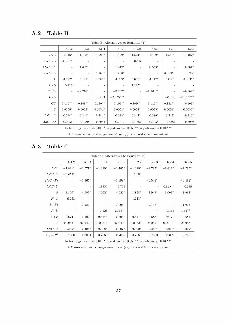
A.2 Table B

Table B: Alternatives to Equation (4)

4.1.2 4.1.3 4.1.4 4.1.5 4.2.2 4.2.3 4.2.4 4.2.5

INC −1.516∗ −1.463∗ −1.525∗ −1.472∗ −1.524∗ −1.489∗ −1.516∗ −1.487∗

INC ·G −0.737∗ - - - 0.0253 - - -

INC · Pr - −1.637∗ - −1.442∗ - −0.559∗ - −0.507∗

INC · U - - 1.950∗ 0.906 - - 0.868∗∗ 0.295

P 4.082∗ 4.181∗ 4.084∗ 4.203∗ 4.040∗ 4.117∗ 4.086∗ 4.133∗∗

P ·G 0.216 - - - 1.227∗ - - -

P · Pr - −2.778∗ - −3.287∗ - −0.563∗∗ - −0.809∗

P · U - - 0.424 −2.0754∗∗ - - −0.404 −1.316∗∗∗

CT 0.110∗∗ 0.109∗∗ 0.110∗∗ 0.109∗∗ 0.109∗∗ 0.110∗∗ 0.111∗∗ 0.109∗

T 0.0056∗ 0.0052∗ 0.0054∗ 0.0052∗ 0.0054∗ 0.0055∗ 0.0051∗ 0.0052∗

INC · T −0.244∗ −0.241∗ −0.244∗ −0.242∗ −0.244∗ −0.239∗ −0.245∗ −0.240∗

Adj −R2 0.7036 0.7039 0.7035 0.7040 0.7038 0.7035 0.7035 0.7036

Notes: Significant at 0.01: *; significant at 0.05: **, significant at 0.10:***

4.X uses economic changes over X year(s); standard errors are robust

A.3 Table C

Table C: Alternatives to Equation (6)

6.1.2 6.1.3 6.1.4 6.1.5 6.2.2 6.2.3 6.2.4 6.2.5

INC −1.821∗ −1.777∗ −1.829∗ −1.785∗ −1.828∗ −1.797∗ −1.821∗ −1.795∗

INC ·G −0.653∗ - - - 0.009 - - -

INC · Pr - −1.565∗ - −1.398∗ - −0.543∗ - −0.492∗

INC · U - - 1.783∗ 0.765 - - 0.849∗∗ 0.288

P 3.899∗ 4.005∗ 3.902∗ 4.029∗ 3.858∗ 3.944∗ 3.903∗ 3.961∗

P ·G 0.252 - - - 1.211∗ - - -

P · Pr - −3.089∗ - −3.663∗ - −0.747∗ - −1.033∗

P · U - - 0.428 −2.365∗∗ - - −0.365 −1.527∗∗

CTE 0.674∗ 0.692∗ 0.674∗ 0.695∗ 0.677∗ 0.683∗ 0.677∗ 0.687∗

T 0.0053∗ 0.0049∗ 0.0051∗ 0.0049∗ 0.0052∗ 0.0052∗ 0.0049∗ 0.0048∗

INC · T −0.389∗ −0.394∗ −0.388∗ −0.397∗ −0.390∗ −0.388∗ −0.389∗ −0.392∗

Adj −R2 0.7060 0.7064 0.7060 0.7066 0.7063 0.7060 0.7059 0.7061

Notes: Significant at 0.01: *; significant at 0.05: **, significant at 0.10:***

6.X uses economic changes over X year(s); Standard Errors are robust

37

A.4 Table D

Table D: One-sided F-tests for sign of inflation and growth relationship for equation (4)

Hypothesis 1 2 3 4

F-statistic 44.69 17.56 16.93 2.71

P > F 1.17× 10−11 1.395× 10−5 1.94× 10−5 0.0497

Hypothesis 5 6 7 8

F-statistic 0.45 17.58 19.71 35.35

P > F 0.25207 1.39× 10−5 4.53× 10−6 1.39× 10−9

Note: df = (1, 29947)

A.5 Table E

Table E: Regression output for equation (8)

8.1.1 8.2.1

Coef. S.E. t P > |t| Coef. S.E. t P > |t|

INC -1.46526 0.031165 -47.02 0 -1.49292 0.031314 -47.68 0

INC ·G -0.49708 0.232955 -2.13 0.033 0.175629 0.16991 1.03 0.301

INC · P -1.51414 0.307409 -4.93 0 -0.60749 0.167267 -3.63 0

P 4.199873 0.031669 132.62 0 4.103187 0.031529 130.14 0

P ·G 0.842985 0.370772 2.27 0.023 1.489718 0.272492 5.47 0

P · P -3.14013 0.476283 -6.59 0 -0.94587 0.246525 -3.84 0

T 0.005564 0.001087 5.12 0 0.005486 0.001088 5.04 0

INC · T -0.13585 0.01317 -10.31 0 -0.13454 0.0132 -10.19 0

Adj −R2 0.704 0.7041

Standard errors are robust; 8.X.1 uses economic changes over X year(s)

38