vot 78237 modeling and simulation of quantum nanostructures for ...
147
VOT 78237 MODELING AND SIMULATION OF QUANTUM NANOSTRUCTURES FOR SINGLE-ELECTRON TRANSISTORS (PEMODELAN DAN SIMULASI STRUKTUR NANO KUANTUM BAGI TRANSISTOR ELEKTRON TUNGGAL) AHMAD RADZI MAT ISA MOHD KHALID KASMIN NOR MUNIROH MUSA PUSAT PENGURUSAN PENYELIDIKAN UNIVERSITI TEKNOLOGI MALAYSIA 2009
Transcript of vot 78237 modeling and simulation of quantum nanostructures for ...

VOT 78237
MODELING AND SIMULATION OF QUANTUM NANOSTRUCTURES FOR SINGLE-ELECTRON TRANSISTORS
(PEMODELAN DAN SIMULASI STRUKTUR NANO KUANTUM
BAGI TRANSISTOR ELEKTRON TUNGGAL)
AHMAD RADZI MAT ISA MOHD KHALID KASMIN NOR MUNIROH MUSA
PUSAT PENGURUSAN PENYELIDIKAN UNIVERSITI TEKNOLOGI MALAYSIA
2009

VOT 78237
MODELING AND SIMULATION OF QUANTUM NANOSTRUCTURES FOR SINGLE-ELECTRON TRANSISTORS
(PEMODELAN DAN SIMULASI STRUKTUR NANO KUANTUM BAGI TRANSISTOR ELEKTRON TUNGGAL)
AHMAD RADZI MAT ISA MOHD KHALID KASMIN NOR MUNIROH MUSA
RESEARCH VOT NO: 78237
Jabatan Fizik Fakulti Sains
Universiti Teknologi Malaysia
2009

i
ACKNOWLEDGEMENTS
First of all, in humble way I wish to give all the Praise to Allah, the Almighty
God for with His mercy has given me the strength, keredhaanNya and time to
complete this work.
I would like to express my sincere gratitude and appreciation to the Ministry
of Higher Education for providing the financial support through FRGS funding.
Thanks are also due to the Research Management Center of Universiti Teknologi
Malaysia for the management of funds VOT No. 78237 for this project.
Thanks also to all my friends and colleagues for their views, concerns,
encouragement and for their continuing support, patience, valuable advices and ideas
throughout the duration of this research.
i
ii
ABSTRACT
Semiconductor clusters have occupied the centre of scientific interest because
of their unique electronic nature. Among the group III-V compound clusters, the
gallium arsenide clusters have been the focus of this research due to their importance
in constructing fast microelectric devices. The electronic structures of gallium
arsenide clusters were studied. The simulations were carried out by using VASP
(Vienna Ab-Initio Software Package) which utilizes the method of density functional
theory (DFT) and plane wave basis set. Gallium arsenide clusters with surface
passivated by hydrogen, GaxAsyHz were simulated to obtain the density of states
(DOS) as well as bandstructure for each cluster. From the DOS graphs, discrete
spectrum was observed instead of bulk-like continuous DOS which is the evolvement
from bulk to nano-size. Bandstructure graphs also showed the discrete energy level
in consistence with the discrete energy spectrum from DOS. It was found that the
bandgaps for hydrogenated gallium arsenide clusters increases with the decrease in
size. Bare gallium arsenide clusters, GaxAsy were also simulated (x + y ≤ 15) gallium
arsenide atoms. Optimization was performed to obtain the ground state structure. The
bandgaps for the ground state gallium arsenide clusters do not show a decreasing
trend with the increment of cluster size as that of hydrogenated gallium arsenide
cluster. The electronic structures of optimized clusters are affected by the surface
orientation of the clusters. Comparison of the bandgap values for GaxAsyHz and
GaxAsy was made.
iii
ABSTRAK
Semikonduktor kluster menjadi matlamat kajian dalam bidang sains
disebabkan oleh sifat elektronik semulajadinya. Antara gabungan kluster kumpulan
III-V, kluster gallium arsenida menjadi tumpuan dalam kajian ini kerana
kepentingannya dalam pembuatan alat-alat mikroelektrik yang lebih pantas. Struktur
elektronik kluster gallium arsenida telah dikaji. Simulasi kajian telah dijalankan
dengan menggunakan perisian VASP (Vienna Ab-Initio Software Package) yang
menggunakan teori fungsian ketumpatan dan set basis gelombang satah. Simulasi ke
atas kluster gallium arsenida yang permukaannya dipasifkan dengan hidrogen,
GaxAsyHz telah dilakukan untuk mendapatkan ketumpatan keadaan dan juga
struktur jalur untuk setiap kluster. Daripada graf ketumpatan keadaan, spektrum
diskrit telah diperolehi. Perubahan ketumpatan keadaan daripada selanjar bagi
struktur pukal ke spektrum diskrit bagi struktur nano merupakan evolusi nano.
Struktur jalur juga menunjukkan aras tenaga diskrit yang selaras dengan spektrum
diskrit daripada ketumpatan keadaan. Jurang jalur untuk gallium arsenida
terhidrogenasi semakin berkurang apabila saiz kluster meningkat. Simulasi ke atas
kluster gallium arsenik tulen (tak terhidrogenasi), GaxAsy yang mempunyai bilangan
atom (x + y ≤ 15) juga dilakukan. Optimasi dilaksanakan untuk mendapatkan
struktur keadaan dasar. Jurang jalur bagi struktur keadaan dasar kluster-kluster itu
tidak mempunyai aliran yang menurun dengan peningkatan saiz kluster seperti yang
berlaku pada kluster gallium arsenida terhidrogenasi. Struktur elektronik kluster-
kluster optimum dipengaruhi oleh orientasi permukaan kluster. Perbandingan nilai
jurang jalur bagi GaxAsyHz dan GaxAsy telah dilakukan.

iv
TABLE OF CONTENTS
CHAPTER TITLE PAGE
ACKNOWLEDGEMENTS
ABSTRACT
ABSTRAK
TABLE OF CONTENTS
LIST OF TABLES
LIST OF FIGURES
LIST OF ABBREVIATIONS
LIST OF SYMBOLS
LIST OF APPENDICES
i
ii
iii
iv
xi
xii
xv
xviii
xxi
1 INTRODUCTION
1.1 Background of Research
1.2 Atomic and Molecular Clusters
1.3 Applications of Clusters
1.4 Introduction to Modeling and Simulation
1.4.1 Modeling and Simulation Approach Used in This
Research
1.5 Research Objectives
1.6 Scopes of Study
1.7 Outline of Dissertation
1
1
2
4
6
8
9
9

v
10
2 COMPUTATIONAL METHOD
2.1 Computational Materials Science (CMS)
2.2 Density Functional Theory
2.2.1 Development of Density Functional Theory
2.2.2 Kohn-Sham Theory
2.2.3 Self-Consistent Field (SCF)
2.2.4 Non-Self Consistent Field
2.2.5 Exchange-Correlation Functionals
2.2.5.1 Local Density Approximation for
Exchange-Correlation Energy
2.2.5.2 Generalized Gradient Approximation (GGA)
2.2.6 DFT Choice of Electronic Structure
2.3 Basis Set
2.3.1 Plane Wave Basis Set
2.3.2 Projected Augmented Wave (PAW) –Pseudopotentials
(PP) in Plane Wave Basis
11
11
16
17
18
22
22
23
23
26
30
32
33
37
3 METHODOLOGY
3.1 Introduction to VASP
3.1.1 Software Packages Needed by VASP
3.2 Files Used by VASP
3.2.1 INCAR File
3.2.2 POTCAR File
3.2.3 POSCAR File
3.2.4 KPOINTS File
3.3 Algorithm Used in VASP
3.3.1 Conjugate Gradient Algorithm
3.3.2 Block Davidson Algorithms
39
39
41
43
44
44
45
45
47
51
52

vi
3.3.3 Residual Minimization Scheme-Direct Inversion In
The Iterative Subspace (RMM-DIIS)
3.4 Simulation Process
3.4.1 Construction of Clusters
3.4.2 Geometry Optimization
3.4.2.1 INCAR for Conjugate Gradient Geometry
Optimization
3.4.2.2 INCAR for Simulate Annealing
3.4.2.3 KPOINTS for Geometry Optimization
3.4.3 Electronic Structures Calculations
3.4.3.1 INCAR for Self-Consistent Run
3.4.3.2 INCAR for Non-Selfconsistent Run
3.4.3.3 KPOINTS for Non-selfconsistent and
Bandstructure
53
54
55
56
58
60
65
65
66
67
68
4 SIMULATION RESULT AND ANALYSIS
4.1 Simulation of Bulk Gallium Arsenide and Gallium Arsenide
Dimer
4.2 The Effect of Size on the Electronic Structures of
Gallium Arsenide Clusters
4.3 The Effect of Shape on the Electronic Structures of Gallium
Arsenide Clusters
4.3.1 Optimized Geometry Structure
4.3.2 Electronic Structures
4.4 Effect of Hydrogen and Reconstructed Surface to Electronic
Structures
69
69
73
80
82
87
102
5 SUMMARY AND CONCLUSION 105
vii
5.1 Summary and Conclusion
5.2 Suggestions
5.2.1 Improvement of the Bandgap Accuracy
5.2.2 Improvement of the Computation Time
105
108
108
109
REFERENCES 113
APPENDICES 121

viii
LIST OF TABLES
TABLE NO TITLE PAGE
1.1 Schematic classification of clusters according to the number N of atoms.
3
2.1 Comparison of accuracy of various computational tools. 31
3.1 A relatively large number of input and output files of VASP.
43
3.2 Coordinates of high symmetry k-points in Cartesian and reciprocal mode.
46
4.1 Bandgap energy for each of the cluster. 77
4.2 The configurations and point group for each of the gallium arsenide clusters, GaxAsy.
82
4.3 Energy level (HOMO and LUMO) as well as bandgap value of each GaxAsy clusters, (x +y ≤ 15 ).
95
4.4 Binding energy per atom of each gallium arsenide cluster, GaxAsy (x + y ≤ 15 ). The binding energies are not corrected with zero potential energies.
96
4.5 Second-difference enegies and electron affinity of each gallium arsenide cluster, GaxAsy (x + y ≤ 15 ).
97
4.6 Bandgap (eV) comparison of bare non-optimized tetrahedral gallium arsenide clusters, hydrogenated gallium arsenide clusters and surface reconstructed gallium arsenide clusters.
102
5.1 Execution time, speedup and efficiency of VASP using parallel computing.
111

ix
LIST OF FIGURES
FIGURE NO TITLE PAGE
1.1 Computational science is defined as the intersection of the three disciplines, i.e. computer science, mathematics and applied science.
8
2.1 Schematic depicting self-consistent loop. 21
2.2 Schematic diagram depicting the energy density for inhomogeneous electron gas system (left hand panel) at any location can be assigned a value from the known density variation of the exchange-correlation energy density of the homogeneous electron gas (right hand panel).
26
2.3 Schematic illustrating the a supercell model for a isolated molecule. The dashed line depicts the boundaries of the supercell.
35
2.4 Schematic representation of a psedopotential (left) and a pseudowavefunction (right) along with all-electron potential and wavefunction. The radius at which all-electron and pseudofunction values match and identical is rc. the pseudofunctions are smooth inside the core region.
36
2.5 Schematic depicting principle of pseudopotential, of which core electrons are neglected.
36
2.6 Schematic depicting the decomposition of exact wavefunction (and energy) into three terms
38
3.1 The First Brillouin zone of a fcc lattice, with high symmetry k-points and direction of planes marked.
46
3.2 Flow chart of iterative methods for the diagonalization of the KS-Hamiltonian in conjunction with an iterative improvement (mixing techniques) of the charge density for the calculation of KS-ground-state.
50

x
3.3 Flow chart of the electronic structure simulation process of gallium arsenide clusters.
55
3.4 (a) Bulk gallium arsenide with its unit cells repeated in 3 dimensions. (b) supercells with Ga2As2 cluster in the center and the distance between clusters is large. The brown’s colour show the Ga atoms and purple’s colour show the As atoms.
56
3.5 Algorithm of geometry optimization used for large clusters.
58
3.6 Parameters for CG algorithm in INCAR file. 59
3.7 Conjugate gradient techniques: (top) Steepest descent step from 0xr search for minimum along by performing several trial steps to
0gr
1xr . (below) New gradient ( )10 xgg rrr
= is determined and 1sr
(green arrow) is conjugated.
60
3.8 Parameters for SA algorithm in INCAR file. 61
3.9 Flowchart illustrating the algorithm of SA. 64
3.10 Parameters for geometry optimization in KPOINTS file. 65
3.11 Parameters for self-consistent run in INCAR file. 66
3.12 Parameters for non-selfconsistent run in INCAR file. 67
3.13 Parameters for non-selfconsistent run in KPOINTS file. 68
4.1 (Left) Structure of zinc blende bulk gallium arsenide; (Right) Structure of Ga1As1.dimer.
70
4.2 Bandstructure of bulk gallium arsenide. 71
4.3 4.4 4.5 4.6
DOS of bulk gallium arsenide Ball and stick model for hydrogenated gallium arsenide clusters. Bandstructrue and DOS of hydrogenated gallium arsenide clusters, GaxAsyHz.
Band shift related to the cluster size. The upper line is HOMO energy value while lower line is LUMO energy value.
72
74
76
77

xi
4.7 Lowest energy geometries for the GaxAsy (x + y ≤ 15).
81
4.8 DOS and bandstructure of Ga1As1 cluster.
88
4.9 DOS and bandstructure of Ga1As2 cluster
88
4.10 DOS and bandstructure of Ga2As2 cluster
89
4.11 DOS and bandstructure of Ga2As3 cluster
89
4.12 DOS and bandstructure of Ga3As3 cluster
90
4.13 DOS and bandstructure of Ga3As4 cluster 90
4.14 DOS and bandstructure of Ga4As4 cluster
91
4.15 DOS and bandstructure of Ga4As5 cluster
91
4.16 DOS and bandstructure of Ga5As5 cluster
92
4.17 DOS and bandstructure of Ga5As6 cluster
92
4.18 DOS and bandstructure of Ga6As6 cluster
93
4.19 DOS and bandstructure of Ga7As6 cluster
93
4.20 DOS and bandstructure of Ga7As7 cluster
94
4.21 DOS and bandstructure of Ga7As8 cluster
94
4.22 Graph of bandgap versus number of gallium arsenide atom in the cluster.
95
4.23 Graph of binding energy per atom of gallium arsenide clusters.
96

xii
4.24 Graph of second-difference enegies and electron affinity of each gallium arsenide cluster, GaxAsy (x + y ≤ 15 ) corresponding to the table above.
97
5.1 Graph of total time used for completing a parallel calculation versus the number of CPU.
111
5.2 Graph of speedup and efficiency vs number of CPU.
112

xiii
LIST OF ABBREVIATIONS
ATLAS - Automatically Tuned Linear Algebra Software
BLAS - Basic Linear Algebra Subprograms
BO - Born Oppenheimer
BP - Becke-Perdew
BSSE - Basis set superposition error
CC - Coupled cluster theory
CG - Conjugate gradient
CI - Configuration Interaction
CMS - Computational materials science
DFT - Density functional theory
DOS - Density of states
ETB - Empirical tight binding
EPM - Empirical pseudopotential method
EMA - Effective mass approximation
FFT - Fast-fourier transform
GEA - Gradient expansion approximation
GGA - Generalized gradient approximation
GTO - Gaussian-type orbital
GVB - Generalized valence bond
HF - Hartree Fock theorem
HK - Hohenberg-Kohn
HOMO - Highest Occupied Molecular Orbital
HPC - High-performance cluster
xiv
IFC - Intel Fortran Compiler
Intel® MKL - Intel Math Kernel Library
KS - Kohn-Sham theorem
LCAO - Linear combination of atomic orbitals
LDA - Local density approximation
LAPACK - Linear Algebra PACKage
LM - Langreth-Mehl
LSDA - Local spin density approximation
LUMO - Lowest Unoccupied Molecular Orbital
LYP - Lee-Yang-Parr
MCSCF - Multi-Configurations Self Consistent Field
MD - Molecular dynamics
MGGA - Meta-Generalized Gradient Approximation
MPI - Message Passing Interface
NC-PP - Norm-conserving pseudopotential
NFS - Network file system
PAW - Projected Augmented Wave
PBE - Perdew-Burke-Ernzernhof
PES - Potential energy surfaces
PP - Pseudopotential
PW - Plane Wave
PW91 - Perdew-Wang 1991
RMM - Residual minimization scheme
rPBE - Revised-Perdew-Burke-Ernzernhof
RPA - Random phase approximation
SA - Simulated annealing
SCF - Self-consistent functional
SSH - Secure Shell
SET - Single-electron transistor
STO - Slater-type orbitals

xv
US-PP - Ultrasoft Vanderbilt pseudopotential
VASP - Vienna Ab-Initio Software Package
VWN - Vosko-Wilk-Nusair
QMC - Quantum Monte Carlo
WF - Wavefunction

xvi
LIST OF SYMBOLS
E - Energy
E - Fermi Energy F
E - Energy gap / bandgap g
E - Exchange-correlation energy XC
f(E) - Fermi energy
F - Force
g(E) - Density of states
g - Spin-scaling factor
G
h
- Reciprocal lattice vector
- Planck’s constant
h - Dirac constant
- Hamiltonian H [nJ ] - Coulomb interaction
k - Wavenumber
k - Boltzmann’s constant BB
L - Edge length
L
( )rn
- Angular momentum operator
m - Mass
n - Quantum number of state (integer)
N - Number of electron r - Electron density
p - Momentum
- Linear momentum operator rp

xvii
εlmp~ - Projector function
r, rr - Position vector
r - Electron spatial coordinates i
r - Wigner-Seitz radius s
( )rRnl
( )ϕ,m
( )r
- Radial wavefunction
R - Radius
R - Nuclei spatial coordinates A
s, t - Dimensionless density gradient
t - time
T - Kinetic energy o
T - Temperature u - Bloch function k
U - Potential Energy
V - Volume
- Spherical harmonic θYl
Z - Nuclei charge A
- λ Wavelength 2 - Second-order difference energy ∆
Ψ - Wavefunction
- υ Velocity
ω - Angular frequency - ν Frequency
- Envelope function φ
- Θ Unit step function
ε - Energy
ε - Single-particle energy level i
μ - Chemical potential
- ∇ Laplacian operator
ξ - Spin-polarization
( )rr - Kinetic energy density τ

xviii
Ω - Volume of unit cell
η - Voltage division factor
ρ - Density matrix
Ga - Gallium
As - Arsenide
GaxAsy - Gallium arsenide cluster with x,y atom
GaxAsyHz - Hydrogenated gallium arsenide cluster with x,y atom and z hydrogen atom
SN - Speedup
EN
- Efficiency

xix
LIST OF APPENDICES
APPENDIX TITLE PAGE
A Parallelization of VASP 113

CHAPTER 1
INTRODUCTION
1.1 Background of Research
In recent years, the structure and properties of microclusters of pure and
compound semiconductors have received much attention and have been the subject
of great interest both for experimental and theoretical studies. The structure and
electronic properties of clusters can be dramatically different from those of the bulk
due to the high surface area to volume ratio. The addition of a few atoms to a cluster
can also result in major structural rearrangement [1].
Studies of clusters become important also because bulk and surface effects
can be modeled using only a few atoms or a supercell of a typical cluster size.
Moreover, with the rapid advancement in science and technology, electronic devices
have been reduced in size and the behavior of semiconductor surface properties has
thus gained more attention. The relation between the geometry and the electronic
structure plays a critical role in dictating the properties of a material.

2
In the case of semiconductors, this evolution is remarkable. Semiconductor
clusters have been shown to exhibit exotic properties quite different from those in
molecules and solids. Compared to homogeneous clusters such as carbon and silicon,
heterogeneous semiconductor clusters like gallium arsenide are more attractive
because their properties can be controlled by changing the composition, in addition
to the size. For these reasons, theoretical studies on clusters are critical to the design
and synthesis of advanced materials with desired optical, electronic, and chemical
properties.
However, theoretical studies of heterogeneous semiconductor clusters have
been limited due to computational difficulties arising from the large number of
structural and permutational isomers formed due to multiple elements. On one hand,
sophisticated computational method such as self-consistent quantum mechanical
calculation is required to make reliable prediction on the properties of these clusters,
in the absence of comprehensive experimental results. On the other hand, the amount
of computational work is enormous in order to find all the stable isomers for a given
cluster size and composition. A number of theoretical and experimental attempts
[2-14] have been made to determine the structure and properties of small GaxAsy
clusters. Most of the theoretical studies have been focused on clusters of a few atoms
due to the above mentioned difficulties.
1.2 Atomic and Molecular Clusters
Study of physical and chemical properties of clusters is one of the most active
and emerging frontiers in physics, chemistry and material science. In the last decade
or so, there has been a substantial progress in generation, characterization and
understanding of clusters. Clusters of varying sizes, ranging from a few angstroms to
nanometers, can be generated using a variety of techniques such as sputtering,
chemical vapor deposition, laser vaporization, supersonic molecular beam etc. Their

3
electronic, magnetic, optical and chemical properties are found to be very different
from their bulk form and depend sensitively on their size, shape and composition.
Thus, clusters form a class of materials different from the bulk and isolated
atoms/molecules. Looking at the mass distribution of clusters, some are found to be
much more abundant than others. These clusters are therefore more stable and are
called magic clusters. They act like superatoms and can be used as building blocks or
basis to form a cluster assembled solid. It is these kinds of developments that add
new frontiers to material science and offer possibilities of designing new materials
with desirable properties by assembling suitably chosen clusters. The Table 1 show
the schematic classification of clusters according to the number N of atoms.
Table 1.1: Schematic classification of clusters according to the number N of atoms.
Observable Very small
clusters
Small clusters Large clusters
Number of atoms N 2 ≤ N ≤ 20 20 ≤ N ≤ 500 500 ≤ N ≤ 107
Diameter d d ≤ 1 nm 1 nm ≤ d ≤ 3 nm 3 nm ≤ d ≤ 100 nm
Surface fraction f undefined 0.5 < f < 0.9 f ≤ 0.5
It should be recognized that if we are to harness full technological potential of
clusters, we have to gain a fundamental scientific understanding of them. This
involves, for example, understanding why clusters are different from atoms and bulk,
what is their geometry and structure and how it evolves with size, the evolution of
their electronic, optical, magnetic and chemical properties with size and the high
stability of some clusters.
Such an understanding will teach us how we can modify the cluster structure
to get a desired property. These are difficult research problems because clusters are

4
species in their own right and do not fall into the field of atoms or solid state. Thus
many techniques of atomic or solid state physics are just not applicable to clusters.
New techniques of applying quantum mechanics have to be developed to handle
clusters. Similarly, thermodynamics of clusters is of great importance. Many
thermodynamical relationships which are derived for the bulk form are not applicable
to clusters. Thus one requires new approaches to concepts of melting, freezing and
phase changes in dealing with finite clusters and their dependence on size. An
understanding of these concepts is important for developing technologies based on
clusters.
Since many cluster properties such as geometry and structure of a cluster are
not directly measurable from experiments, theoretical models and computation play
an important role in the study of clusters. In this respect, the Density Functional
Theory (DFT) which is designed to handle a large number of electrons quantum
mechanically, has been found to be extremely useful. Using this theory one can
calculate very accurately the total energy and other properties of a many electron
system in its ground state ( ground state energy is the lowest energy of a system;
lately, the DFT has also been developed to calculate excited states).
1.3 Applications of Clusters
Clusters are an important state of matter, consisting of aggregates of atoms
and molecules that are small enough not to have the same properties as the bulk
liquid or solid. Quantum states in clusters are size-dependent, leading to new
electronic, optical, and magnetic properties. Clusters offer attractive possibilities for
innovative technological applications in ever smaller devices, and the ability to
"tune" properties, especially in semiconductors, may produce novel electronic and
magnetic capabilities.

5
Semiconductors are one of the most active areas of cluster research. Many of
their properties are very dependent on size; for example, optical transitions can be
tuned simply by changing the size of the clusters. Alivisatos [15] describes current
research on semiconductor clusters consisting of hundreds to thousands of atoms--
"quantum dots." These dots can be joined together in complex assemblies. Because
of the highly specific interactions that take place between them, a "periodic table" of
quantum dots is envisioned. Such coupled quantum dots have potential applications
in electronic devices.
The magnetic properties of clusters are of fundamental interest and also offer
promise for magnetic information storage. Shi et al. [16] describe recent
developments in the study of magnetic clusters, both isolated and embedded in a host
material. Such clusters can behave like paramagnets with a very large net moment--
superparamagnets. Superparamagnetic particles can be embedded in a metal and
show dramatic field changes in electrical conduction. Ion implantation has generated
ferromagnetic clusters embedded in a semiconductor host, which can be switched
individually.
The constituents of clusters can be arranged in many different ways: Their
multidimensional potential energy surfaces have many minima. Finding the global
minimum can be a daunting task, to say nothing of characterizing the transition states
that connect these minima. Wales [17] describes the fundamental role of the potential
energy surface in the understanding of the structure, thermodynamics, and dynamics
of clusters. In a Report accompanying the special section, Ball et al. [18] analyze
Ar19 and (KCl)32 clusters and illustrate how potential energy surface topography (the
sequences of minima and saddles) governs the tendency of a system to form either
amorphous or regular structures.
Water is essential to life and to a great number of chemical processes.
Hydrogen bonding, the source of many of water's most interesting properties,
requires at least two water molecules. Far-infrared laser vibration-rotation tunneling
6
experiments on supersonically cooled small clusters allow characterization of
geometric structures and low-energy tunneling pathways for rearrangement of the
hydrogen bond networks. Liu et al. [19] describe how these and other recent
experiments on water clusters give insight into fundamental properties of water.
Simple aggregates of carbon atoms, especially C60, are remarkably stable.
Determination of their actual physical and electronic structures is a formidable task
because of the large number of electrons and the many possible isomeric
arrangements involved. Scuseria [20] reviews the status of the field, including recent
advances and current challenges in ab initio algorithms.
1.4 Introduction to Modeling and Simulation
Modeling is the technique of representing a real-word system or phenomenon
with a set of mathematical equations or physical model. A computer simulation then
attempts to use the models on a computer so that it can be studied to see how the
system works. Prediction may be made about the behavior and performance of the
system by changing its variables. In this research, nanostructures are the system
targets of the modeling and simulation.
Simulation is a useful and important part of modeling nanostructures to gain
insight into the attributes of a structure or a whole system with several structures
connected. It is a method to predict the behavior transformation for a variable
changing before performing a practical experiment. The simulation can then be
proven by the results of experiment. This is also a beneficial approach to test the
most optimal and the best performance of a device which is built by those
nanostructures before the real fabrication.

7
Besides, simulation can give detailed theoretical explanation to the
phenomenon that could not be solely explained by experiment . Among the examples
are the reconstruction of the small cluster structures and the occupation of the
electrons. With the 3D graphical viewer and animation, we can view the atomic
structure models and the process of the structure transformation. With computer
simulation done prior to experiment, the mastering of the small cluster structures
principles is improved and ‘trial and error’ could be reduced during experiment.
However, there isn’t a comprehensive simulator which can take into account
every factor that would contribute to the system changes. Many of those only adopt
the approximation which is the most optimal and closest to the real system for the
representation. For nanostructures, first principle calculation is an appropriate
simulation approach for studying the electronic structures and properties. The
advantage of this calculation is that, it can be done without any experimental data.
However, it could be a massive calculation that consumes a very long time to
accomplish.
Computational science becomes an essential tool in modeling and simulation.
It is the application of computational and numerical technique to solve large and
complex problem, for example, complex mathematics that involved a large number
of calculations. Therefore, modeling and simulation are commonly accomplished by
the aid of computational science and therefore they are always referred to computer
modeling and computer simulation. Computational science could be defined as an
interdisciplinary approach that uses concepts and skills from the science, computer
science and mathematic disciplines to solve complex problems which allow the study
of various phenomena. It can be illustrated by Figure 1.1. To improve the
performance and speed of large computation, one of the approaches is parallel
computing. Parallel computing can reduce the computing time of computational
costly calculations such as first principle calculations mentioned above, where it
distributes the calculation to two or more processors or computers.

8
Mathematics Applied Science
1.4.1 Modeling and Simulation Approach Used in This Research
In this research, Vienna Ab-initio Simulation Package (VASP) is used as the
simulation tools for electronic structures of the gallium arsenide clusters. VASP is
the leading density functional code to accurately compute structural, energetical,
electronic and magnetic properties for a wide range of materials including solids and
molecules. VASP is highly efficient for structural optimizations and ab-initio
molecular dynamics (MD). It covers all elements of the periodic table of practical
interest. With its projector-augmented-wave (PAW) potentials, VASP combines the
accuracy of all electron methods with the elegance and computational efficiency of
plane wave approaches.
Computational science
Computer Science
Figure 1.1: Computational science is defined as the intersection of the three disciplines, i.e. computer science, mathematics and applied science.

9
1.5 Research Objectives
The main interest of this research is to study the electronic structures of
gallium arsenide clusters. The objectives of this research can be summarized as the
following:
a) to study the electronic structures of gallium arsenide clusters with variable
size and structures.
b) to study the relation between the bandgap and the structures size of the
gallium arsenide clusters.
1.6 Scopes of Study
The scopes of this research are as the following:
a) Clusters is simulated as isolated small range nanocluster.
b) Gallium arsenide is adopted as the material of the clusters.
c) Bandstructures and energy spectrum are studied for the electronic structures
of gallium arsenide clusters.
d) Density functional theory is used to calculate and simulate the electronic
structures of gallium arsenide clusters.

10
1.7 Outline of Thesis
A general background of study and brief introduction to clusters are discussed
in Chapter 1. This is followed by introduction of modeling and simulation, objective
and scope of study. There are a lot of approaches to simulate the electronic structures
of gallium arsenide clusters. Density functional theory (DFT) is a sufficient method
in doing this. Its theory is discussed in the Chapter 2. The methodology of the
simulation VASP which is utilized in this study is introduced in Chapter 3.
Following this, Chapter 4 would be results and discussion. Figures and graphs of the
electronic structures of gallium arsenide clusters are showed and the results are
discussed and interpreted. Finally Chapter 5 which is the conclusion. Theories and
results discussed in the previous chapters are summarized and concluded here.
Furthermore, suggestion is given on how to make the simulation better and more
complete.

CHAPTER 2
COMPUTATIONAL METHOD
Electronic structure and stability of gallium arsenide clusters were investigated in
detail by several theoretical studies based on Hartree-Fock (HF) [21,22], density
functional theory (DFT) [6,23], configuration interaction theory (CI) [24,25] and the
ab initio molecular dynamics Car-Parrinello method [5]. For this research, gallium
arsenide clusters GaxAsy (x+y≤15) are investigated using the density functional
theory. Density functional theory is the computational method used in the simulation
tool. This chapter gives a basic understanding on the relevant theorem used, although
it had been well developed for the simulation tool. The next chapter will describe the
simulation tool itself.
2.1 Computational Materials Science ( CMS)
Computational materials science (CMS) is an interdisciplinary research area
of physics, chemistry and scientific computing [26]. It can bring a microscopic
understanding of the interrelationship between structure, composition, and various
materials properties through classical and quantum mechanical modeling. As
discussed above, we are dealing with quantum theory when the structures are in

12
nano-scale. Therefore, solution of Schrödinger equation, which model molecules in
mathematics, brings understanding of the properties of nanostructures. By using
Schrödinger equation, one can implement the following tasks:
i. electronic structure determinations
ii. geometry optimizations
iii. electron and charge distributions
iv. frequency calculations
v. transition structures
vi. potential energy surfaces (PES)
vii. chemical reaction rate constants
viii. thermodynamic calculations e.g. heat of reactions, energy of
activation
Theoretical techniques of CMS with regards to Schrödinger equation can be
generally categorized into three methods: molecular mechanics, semi-empirical or
empirical, and ab-initio methods.
Molecular mechanics is referred to the use of Newtonian mechanics to model
molecular systems. It is a mathematical formalism which produces molecular
geometries, energies and other features by adjusting bond lengths, bond angles and
torsion angle to equilibrium values that are dependent on the hybridization of an
atom and its bonding scheme. The potential energy of the system is calculated using
force field. In molecular mechanics, a group of molecules is treated as a classical
collection of balls and springs rather than a quantum collection of electron and nuclei.
Hence, each atom is simulated as a single particle with assigned parameters as radius,
polarizability, net charge, ‘spring’ length (bond length). These parameters are
generally derived from experimental data or ab-initio calculations beforehand. In
many cases, large molecular systems can be modelled successfully with molecular
mechanics, avoiding quantum mechanical calculations entirely.

13
Semi-empirical is defined as ‘partly from experiment’. Semi-empirical and
empirical methods are based on the Hartree Fock formalism that is simplified using
empirical data derived from experimental, to make approximations and consequently
to improve performance. They are important in treating large molecules where the
full Hartree Fock method without approximations is too costly. Electron correlation
is included in this method with the use of empirical parameters. In this method, one
of the approximations is that two-electron integrals involving two-center charge
distributions are neglected or parameterized and only valence shell electrons are
considered. The rationale behind this approximation is that the electrons involved in
chemical bonding or other phenomena are those in the valence shell.
Parameterization is done to correct the loss, that the results are fitted by a set of
parameters, normally in such a way as to produce results that best agree with
experimental data, but sometimes to agree with ab-initio results. Empirical tight
binding (ETB), empirical pseudopotential method (EPM), and k · p approximation or
its equivalent form of effective mass approximation (EMA) are those among semi-
empirical electronic structure methods [27]. Semi-empirical calculations are faster
than their ab-initio counterpart.
The next level is ab-initio method which means ‘from the beginning’ in Latin.
As opposed to semi-empirical, ab-initio do not include any empirical or semi-
empirical in their equation but being derived directly from theoretical principles
without inclusion of experimental data. It could be also known as first principle.
This does not imply that Schrödinger equation have to be solved exactly, but
reasonable approximation to its solution is made by choosing a suitable method and a
basis set that will implement that method in a reasonable way is selected. Usually the
approximations made are mathematical approximations. The time-dependent, non-
relativistic Schrödinger equation can be written as
( ) ( )AiAi R,rER,rH ψψ = , (2.1)
where H is the Hamiltonian operator with the total energy E as eigenvalue and many-
wavefunction ψ(ri, RA) as eigenfunction with ri is electron spatial coordinates and RA

14
is nuclei spatial coordinates [28]. The Hamiltonian operator with N electrons and M
nuclei in atomic unit (me = e = ħ = 1) is given by
∑ ∑∑ ∑∑ ∑∑∑= = = = > = >=
++−∇−∇−=M
A
N
i
M
A
N
i
N
ij
M
A
M
AB AB
BA
jiiA
AA
A
N
ii R
ZZrr
Zm
H1 1 1 1 1
2
1
2 1121
21 . (2.2)
Indices i and j run over N electrons while A and B over the M nuclei. is the
Laplacian operator acting on particle, m
2∇
A is the mass of nuclei A and ZA is its nucleus
charge, rij is the distance between particle i and j which is equal to | ri – rj |, and same
to riA. The first term in equation (2.2) is the operator for the kinetic energy of the
electrons; the second term is the operator for the kinetic energy of the nuclei; the
third term represents the coulomb attraction between electrons and nuclei; the fourth
term represents the repulsion between electrons and the last term represents repulsion
between nuclei [29]. The wavefunction ψ is then a function of (3N+3M) spatial
coordinates for a system containing N electrons and M nuclei. This is a very
complicated problem that is impossible to be solved exactly. The first step in
simplifying this problem is the Born Oppenheimer (BO) approximation. Since the
nuclei are much heavier than electrons, they move more slowly. Hence, a good
approximation can be made by considering the electrons in a molecule to be moving
in the field of fixed nuclei [29]. As a result, the second term of equation (2.2) can be
neglected and the last term can be considered to be a constant which has no effect on
the operator eigenfunctions. Then the remaining terms are called the electronic
Hamiltonian which is given by
∑∑ ∑∑∑= = = >=
+−∇−=N
i
M
A
N
i
N
ij jiiA
AN
iielec rr
ZH1 1 11
2 121 . (2.3)
Although BO simplifies the original Schrödinger, the electronic part is still a
daunting task to be solved exactly for systems with more than a few electrons and
further approximation must be introduced. One fundamental approach is the Hartree
Fock (HF) scheme, in which the principal approximation is called the central field
approximation which means the Coulombic electron-electron repulsion is not
specifically taken into account. Only its net effect is included in the calculation. As a
result, the energies from HF calculation are always greater than the exact energy and
tend to a limiting value called Hartree Fock limit. Post-Hartree-Fock methods which

15
are used by many calculations, begin with a Hartree-Fock calculation and
subsequently correct for electron-electron repulsion, referred to also as electronic
correlation. Some of these methods are Møller-Plesset perturbation theory (MPn,
where n is the order of correction), the Generalized Valence Bond (GVB) method,
Multi-Configurations Self Consistent Field (MCSCF), Configuration Interaction (CI)
and Coupled Cluster theory (CC). Other important formalism which treats the
correlation energy is Density Functional Theory (DFT) which has become popular in
last two decades. In this method, energy is expressed as a function of total electron
density. DFT is selected as the method of electronic structure in this research. It will
be explained in more detailed in the following. Another method of ab-initio is
Quantum Monte Carlo (QMC) which avoids making the HF mistakes in the first
place. QMC methods work with an explicitly correlated wave function and evaluate
integrals numerically using a Monte Carlo integration. Although these calculations
can be very time consuming, they are probably the most accurate methods known
today. As these methods are pushed to the limit, they approach the exact solution of
the non-relativistic Schrödinger equation. Relativistic and spin-orbit term should be
included to obtain exact agreement with experiment.
In HF, each molecular orbital is expanded in terms of a set of basis functions
which are normally centered on the atoms in the molecule, as given by LCAO
equation. The basis functions collectively are the basis set. Ab-initio is a method of
calculation involves a choice of method and a choice of basis set. It offers a level of
accuracy one needs to understand most physical properties of various materials.
However in comparison with semi-empirical or empirical method, the high degree of
accuracy and reliability of ab-initio calculation is compensated by large
computational demand. In this method, the total molecular energy can be evaluated
as a function of the molecular geometry, or in other words the potential energy
surface.
16
2.2 Density Functional Theory
Density Functional Theory (DFT) is among the most popular and versatile
methods in condensed matter physics or computational physics as well as
computational chemistry. It is a quantum mechanical method that is widely used to
investigate the electronic structure of many-body systems, particularly molecules and
condensed phases. The contribution of DFT was given a great assurance with the
award of the 1998 Nobel Prize in Chemistry to Walter Kohn and John Pople. DFT
has been applied most of all to systems of electrons like atoms, molecules, clusters,
homogenous solids, surfaces and interfaces, quantum wells, quantum dots and others
[30]. It includes a significant fraction of the electron correlation for about the same
cost of doing a HF calculation. Strictly speaking, DFT is neither a HF method nor
post-HF method. The wavefunctions for spin and spatial parts are constructed in a
different way from those in HF and the induced orbitals are often referred to as
‘Kohn-Sham’ orbitals. Nonetheless, the same procedure of SCF is used as in HF
theory.
The main objective of density functional theory is to replace the many-body
electronic wavefunction with the electronic density as the basic quantity. The many
body Schrodinger equation is similar to equation (2.1) but can be more explicitly
shown by
( ) ( )NN rrrErrrH rL
rrrL
rr ,,,, 2121 ψψ = (2.4)
The particle density which is the key variable in DFT is given by
( ) ( ) ( NNN rrrrrrrdrdrdNrn )rL
rrrL
rrL
r ,,,,,,*2121
33
32
3 ψψ∫ ∫∫= (2.5)
The electron density only depends on 3 instead of 3N spatial coordinates, but still
contains all the information needed to determine the Hamiltonian, for example
number of electron N, the coordinate of nuclei RA and the charge of nuclei ZA. This is
the advantage of electron density compared to wavefunction. N is simply given by
the integral over ( )rn r :
( )∫ = Nrdrn 3r (2.6)

17
2.2.1 Development of Density Functional Theory
The very first attempt to use electron density ( )rn r to calculate its total energy
is the Thomas-Fermi theory formulated by Thomas and Fermi in 1927 [31,32]. They
calculated the energy of an atom by representing its kinetic energy as a functional of
the electron density, combining this with the classical expression for the nuclear-
electron and electron-electron interactions. Thus, Thomas-Fermi model is the
predecessor to density functional theory. However, Thomas-Fermi model is not very
accurate since there is no exchange or correlation included, and also the Thomas-
Fermi kinetic energy functional is only a crude approximation to the actual kinetic
energy. Hohenberg-Kohn justified in 1964 the use of electron density as basic
variable in determining total energy. They gave a firm theoretical footing to DFT
with two remarkable powerful theorems. The first Hohenberg-Kohn theorem proved
that the relation expressed in equation (2.5) can be reversed, in which the ground
state wavefunction ( No rrr )rL
rr ,, 21ψ can be calculated by a given ground state density
with a unique functional as shown below : ( )rnor
[ ]ooo nψψ = (2.7)
It shows that there exists the one-to-one mapping between ground state electron
densities and external potentials. Therefore, ground state energy is given by
[ ] [ ] [ ]oooooo nHnnEE ψψ== (2.8)
By substituting equation (2.3), we may represent the energy as:
[ ] [ ]( [ ]))()()()()( 3 rnVrnTrdrVrnrnE eeeextrrrrr
−++= ∫ (2.9)
where is equal to the interaction of the electrons with the nuclei V)(rVextr
N-e and it is
non-universal, while [ ] [ ] [ ]nVnTnF eeeHK −+= is the Hohenberg-Kohn functional
which does not depend on external potential and is therefore universal. The
minimization of the energy functional shown in equation (2.9) will yield ground state
density and thus all other ground state observables. The exact form of has
not been found and thus approximation must be used for the variational principle that
was introduced in the second Hohenberg-Kohn theorem. The variational problem of
on [ ]nFHK

18
minimizing the energy functional [ ]nE can be solved by applying the Lagrangian
method of underdetermined multipliers, which was done by Kohn-Sham.
2.2.2 Kohn-Sham Theory
In year 1965 which is a year after the Hohenberg-Kohn theorem was published,
Kohn and Sham proposed a method to obtain an exact, single-particle like,
description of a many body system by approximation of universal HK functional FHK.
Kohn and Sham separate FHK into three parts so that ( )[ ]rnE r becomes
[ ] [ ] [ ] [ ]nEnJnTnF XC++= 0 (2.10)
( )[ ] ( )[ ] ( ) ( ) ( )[ ] ( ) ( )∫∫∫ ++′′−′
+= rdrVrnrnErdrd|rr|
rnrnrnTrnE extXC333
0 21 rrr
rr
rrrr (2.11)
where is the kinetic energy of the non-interacting electron gas with density ( )[ rnT r0 ]
( )rn r, the second term is the Hartree potential which describes coulomb interaction
between electrons, is the exchange-correlation energy. is calculated
in terms of the
( )[ rnEXCr ] [ ]nT0
( )rirφ ’s
( )[ ] ( ) ( ) rdrr*rnT ii
i32
0 21 rrr φφ ⎟
⎠⎞
⎜⎝⎛ ∇−= ∑∫ (2.12)
Though is not the exact kinetic energy, it is well defined and is treated exactly
in this method. This eliminates some of the shortcomings of the Thomas-Fermi
approximation to the Fermion system, for instances the lack of shell effects or
absence of the bonding in molecules and solids. In equation (2.11), is the
only term can not be treated exactly and thus it is the only term concerned in the
approximation of that equation. By applying variational principle, equation (2.11)
can be written in terms of an effective potential,
[ ]nT0
( )[ rnEXCr ]
( )rVeffr as follow:
( )[ ]( ) ( ) μ
δδ
=+ rVrnrnT
effr
r
r0 (2.13)

19
where ( ) ( ) ( ) ( )[ rnrd|rr|
rnrVrV XCexteffr
rr ]r
rr μ+′′−′
+= ∫ 3 (2.14)
and ( )[ ] ( )[ ]( )rn
rnErn XC
XC r
rr
δδ
μ = (2.15)
μ is the Lagrange multiplier related to the conservation of N and ( )rVeffr is called
Kohn-Sham (KS) effective potential. If one consider a system that contains non-
interacting electrons that is without any two-body interaction, moving in an external
potential ( )rVeffr as defined in equation (2.14), then the same analysis will lead to the
exactly same equation (2.13). Solution of equation (2.13) can be found by solving
single-particle equation for the non-interacting particles (KS equation):
( ) ( ) ( )rrrV iiieffrrr φεφ =⎟⎟
⎠
⎞⎜⎜⎝
⎛+
∇−
2
2
(2.16)
where iε is the Kohn-Sham eigenvalue which is the Lagrange multipliers
corresponding to the orthonormality of the N single-particle states ( )rirφ referring to
the variational condition under the orthonormality constraint jiji δφφ = which
lead to the following equation:
( )[ ] ( ⎥⎦
⎤⎢⎣
⎡−− ∑
j,ijijijirnE δφφεδ r ) = 0 (2.17)
The density is constructed from a set of one-electron orbitals or called Kohn-Sham
orbitals (non-interacting reference system):
( ) ( )∑=i
i |r|rn 2rr φ (2.18)
Since the Kohn-Sham potential ( )rVeffr depends upon the density ( )rn r
, equation
(2.14)-(2.16) must be solved self-consistently. This can be done by making a guess
for the form of the density, then Schrödinger equation is solved to obtain a set of
orbitals ( ) rir φ from which a new density is constructed and the process repeated
until the input and output densities are the same as depicted in Figure 2.1. Practically
there is no problem of converging to the ground state minimum owing to the convex
nature of density functional. From this solution, ground state energy and density can
be determined. Total energy is then given by:
( ) ( ) ( )[ ] ( )[ ] ( )∫∑ ∫∫ −+′′−′
−= rdrnrnrnErdrd|rr|
rnrnE XCXCi
i333
21 rrr
rr
rr
με (2.19)

20
where ( ) ( )[ ] ( ) ( )∑ ∫∑ +=+∇
−=i
effi
ieffii rdrnrVrnTrV 30
2
2rrrr φφε (2.20)
In the above equation, ∑i
iε is the non-interacting system energy which given by the
sum of one-electron energies and when double-counting correlations is included
which double-counts the Hartree energy and over-counts the exchange-correlation
energy, induces the interacting system energy E. The solution of equation (2.13) and
(2.15) is much simpler than that of the HF equation since the effective potential is
local.
KS theory succeeds to transform N-body problem into N single-body
problem with each coupled to Kohn-Sham effective potential. In contrary to HF,
there is no physical meaning of these single-particle Kohn-Sham eigenvalues and
orbitals but are merely mathematical tools that facilitate the determination of the true
ground state energy and density. In HF theory, Koopman’s theorem provide a
physical interpretation of orbital energies iε such that the orbital energy is an
approximation of the negative of the ionization energy associated with the removal
of an electron from orbital iφ which is given by
( ) ( ) ( )iIEnEnE iHF
iHFHF
i −==−== 01ε . It explains that the ionization potentials
and electron affinities are approximated by the negative of the HF occupied and
virtual orbital eigenvalues respectively. It assumes no relaxation of the orbitals when
occupation numbers are changed. This theorem is invalid for KS orbitals in which
the total energy is a nonlinear functional of the density as derived from equation
(2.16).
( )[ ]( ) ( ) ( ) ( )rrrn,rnrnE
iiiii
rrrr
r
φφεδδ *== (2.21)
The exception is the highest occupied KS eigenvalue for which it has been shown to
be the negative of the first ionization potential. Also, DFT is only variational if the
exact energy functional is used, yet HF theory is variational providing an upper
bound to the exact energy.

21
Vext known / constructed
Initial guess ( )rn r
Calculate J[n] and EXC[n]
( ) ( ) ( ) ( )rrrVrH iiieffirrrr φεφφ =⎟⎟
⎠
⎞⎜⎜⎝
⎛+
∇−=
2
2
Calculate new ( ) ( )∑= i |r|rn 2rr φ
Self-Consistent ?
Problem solved. Can now calculate energy, forces, etc.
Generate new ( )rn r
Problem diagonalizing
Problem mixing
No
Yes
Figure 2.1: Schematic depicting self-consistent loop.

22
2.2.3 Self-Consistent Field (SCF)
A self-consistent field (SCF) procedure used to find approximate wave
functions and energy levels in many electron atoms. This procedure was introduced
by the English mathematician and physicist Douglas Hartree in 1928 and improved
by the Soviet physicist Vladimir Fock in 1930 ( by taking into account the Pauli
exclusion principle). The initial wave functions can be taken to be hydrogenic atomic
orbitals. The resulting equations can be solved numerically using a computer. The
results of the Hartree-Fock theory are sufficiently accurate to show that electron
density occurs in shells around atoms and can be used quantitatively to show
chemical periodicity.
2.2.4 Non-Self Consistent Field
Recently there was an increased interest in the so called Harris-Foulkes (HF)
functional. This functional is non- self consistent: The potential is constructed for
some 'input' charge density, then the band-structure term is calculated for this fixed
non- self consistent potential. Double counting corrections are calculated from the
input charge density: the functional can be written as
[ ] ( ) ( )[ ] [ cinc
inxc
in
H
in
xc
in
H
ininHF ETrurebandstructE VVVV ρρρρρ α ++−−++= 2/, ] (2.22)
It is interesting that the functional gives a good description of the binding-energies,
equilibrium lattice constants, and bulk-modulus even for covalently bonded systems
like Ge. In a test calculation we have found that the pair-correlation function of l-Sb
calculated with the HF-function and the full Kohn-Sham functional differs only
slightly. Nevertheless, we must point out that the computational gain in comparison

23
to a self consistent calculation is in many cases very small (for Sb less than 20%).
The main reason why to use the HF functional is therefore to access and establish the
accuracy of the HF-functional, a topic which is currently widely discussed within the
community of solid state physicists. To our knowledge VASP is one of the few
pseudopotential codes, which can access the validity of the HF-functional at a very
basic level, for example without any additional restrictions like local basis-sets and
others. Within VASP the band-structure energy is exactly evaluated using the same
plane-wave basis-set and the same accuracy which is used for the self consistent
calculation. The forces and the stress tensor are correct, insofar as they are an exact
derivative of the Harris-Foulkes functional. During a MD or an ionic relaxation the
charge density is correctly updated at each ionic step
2.2.5 Exchange-Correlation Functionals
The results so far are exact, provided that the exchange-correlation functional
is known. The problem of determining the functional form of the universal
HK density functional F
( )[ rnEXCr ]
HK, has now been transferred to the exchange-correlation
functional of Kohn-Sham formalism, and therefore this term is not known exactly.
Good approximation for ( )[ ]rnEXCr is still one of the challenge’s aims in modern
DFT.
2.2.5.1 Local Density Approximation for Exchange-Correlation Energy
The simplest approximation for exchange-correlation functional is local
density approximation (LDA), which works well and most widely used. This
approximation assumes that the density can be treated locally as a uniform electron
gas which describes a system in which electrons move on uniform positive
24
background charge distribution such that overall charge neutrality is preserved. The
exchange-correlation energy at each point in the system is the same as even if the
inhomogeneity is large by approximating it locally with the density of homogeneous
electron gas (see Figure 2.2). This approximation was firstly formulated by Kohn and
Sham and holds for a slow varying density. Using this approximation, the exchange-
correlation energy for a density is commonly written as
( )[ ] ( ) ( )[ ]∫= rdrnrnrnE LDAXC
LDAXC
3rrr ε (2.23)
where ( )[ rnLDAXC ]rε is the exchange-correlation energy density corresponding to a
homogeneous electron gas with the local density ( )rn r. The energy is again can be
separated into exchange and correlation contribution:
( )[ ] ( ) ( )[ ] ( ) ( )[ ]∫∫ += rdrnrnrdrnrnrnE LDAC
LDAX
LDAXC
33 rrrrr εε (2.24)
The LDA exchange-correlation potential is yielded by the functional derivatives of
equation (2.23):
( ) ( )[ ]( ) ( )[ ] ( ) ( )[ ]
( )rnrn
rnrnrn
rnEr
LDAXCLDA
XC
LDAXCLDA
XC r
rrr
r
rr
δεδ
εδ
δμ +== (2.25)
The available exchange and correlation potential of LDA type are as follow:
• Dirac-Slater exchange [33].
• Vosko-Wilk-Nusair (VWN) correlation [34].
• Vosko-Wilk-Nusair (VWN) correlation within the random phase
approximation (RPA) [34].
• Perdew and Zunger parametrization of the homogenous electron gas
correlation energy, which is based on the quantum Monte Carlo calculations of
Ceperley and Alder [35].
The exchange part of the energy per particle ( )[ ]rnLDAX
rε is given by Dirac functional:
( )[ ] ( )3
13
43
⎟⎠⎞
⎜⎝⎛−= rnrnX
rr
πε (2.26)
Accurate results of correlation energy per particle ( )[ ]rnLDAC
rε have been given by
Quantum Monte Carlo (QMC) calculations of Ceperly and Alder [36] for
homogenous electron gas of different densities. This is the most common correlation
formula used. Other methods finding correlation is listed above. Perdew and Zunger
proposed the formula:

25
( )⎩⎨⎧
>++≤+++
=111
21 sss
sssssPZC rrr
rrDrlnrCBrlnAββγ
ε (2.27)
where rs is the Wigner-Seitz radius of each electron. For high-density (rs ≤1), RPA is
used to obtain the parameters for LDA. For intermediate regime of densities, the
simplest approach to the correlation energy is an interpolation between the high- and
the low limit-density. Another widely used VWN correlation is given as:
( ) ( ) ( )( )
⎥⎥
⎦
⎤
⎢⎢
⎣
⎡
⎟⎟
⎠
⎞
⎜⎜
⎝
⎛
+
−
−
−+⎟⎟⎠
⎞⎜⎜⎝
⎛ −−⎟⎟
⎠
⎞
⎜⎜
⎝
⎛
+
−
−+⎟⎟⎠
⎞⎜⎜⎝
⎛= −−
brbc
tanbc
xbrFxr
lnxFxb
brbc
tanbc
brF
rlnA ss
s
ss
sVWNC
21
200
0
02
1
2
4
4
2224
4
2ε (2.28)
F(x) = x2 + bx + c and other filling parameter, which varies for polarized and
unpolarized conditions are obtained by the data of Ceperly and Alder.
Most of the Kohn-Sham calculations were carried out under the LDA which
produces surprisingly accurate results which makes it widely used especially in solid
state physics. In LDA, exact properties of exchange-correlation hole are maintained.
The electron-electron interaction depends only the spherical average of exchange-
correlation hole and this is reasonably well reproduced. The errors in exchange and
correlation energy densities tend to cancel each other. Properties such as structure,
vibrational frequencies, phase stability and elastic moduli are described reliably for
many systems. However it tends to underpredict atomic ground state energies and
ionisation energies, while overestimating binding energies (typically by 20-30%).
Results obtained with the LDA usually become worse with the increasing
inhomogeneity of the described system such as in atoms or molecules particularly.
Nevertheless, the astonishing fact is that the LDA works as well as it does give the
reduction of the energy functional to a simple local function of the density.

26
Figure 2.2: Schematic diagram depicting the energy density for inhomogeneous electron gas system (left hand panel) at any location can be assigned a value from the known density variation of the exchange-correlation energy density of the homogeneous electron gas (right hand panel).
( )rn r
rr
( )rn r
[ ]nXCε
2.2.5.2 Generalized Gradient Approximation (GGA)
As stated above, the LDA uses the exchange-correlation energy of the
homogeneous electron gas at every point in the system regardless of the homogeneity
of the real charge density. For nonuniform or inhomogeneous charge densities the
exchange-correlation energy can deviate significantly from the homogeneous result.
An improvement to this deviation is by considering the gradient of the charge density,
which is utilized by Generalized Gradient Approximation (GGA). GGA was
developed from gradient expansion approximation (GEA) proposed by Hohenberg
and Kohn [37]. In comparison with LSDA, GGA tends to improve total energies,
atomization energies, binding energies, bond length and angle [38], energy barriers
and structural energy difference. Differ from the LDA which is local, GGA is semi-
local functional. General semi-local approximation to the exchange-correlation
energy as a functional of the density and its gradient to fulfill a maximum number of
exact relations is given by:
[ ] ( )∫ ∇∇= rdn,n,n,nfn,nE GGAXC
3βαβαα β (2.29)
where f is the analytic function. There are two strategies for determining function f.
The first one is known as non-empirical by adjusting f such that it satisfies all known
properties of the exchange-correlation hole and energy (Perdew); and the second way
is semiempirical by fitting f to a data-set containing exactly known binding energies

27
of atoms and molecules (Becke). Many GGA’s are tailored for specific classes of
problems, among those are: Langreth-Mehl 1983 (LM) [39,40], Perdew-Wang 1986
(PW86) [41,42], Becke-Perdew 1988 (BP) [43], Lee-Yang-Parr 1988 (LYP) [44],
Perdew-Wang 1991 (PW91) [45,46], Perdew-Burke-Ernzernhof 1996 (PBE) [47,48],
and Revised-Perdew-Burke-Ernzernhof 1999 (rPBE) [49].
One way to compare these GGA’s (for spin-polarized system) is to define the
exchange-correlation energy in terms of enhancement factor [42] as: [ s,rF sGGA
X ]
[ ] ( ) ( )[ ] ( ) ( )[ ]∫= rdrs,,rrFrnrnn,nE sLDAX
GGAXC
3rrrr ξεβα (2.30)
where ( )[ ] πε 43 FLDAX krn −=
r is the exchange energy per particle for a uniform gas
of density n, which is defined by the LDA, s is a dimensionless measure of the
gradient
( ) ( )( ) ( )rnrk
|rn|rsF
rr
rr
2∇
= (2.31)
with the local Fermi wavevector defined as
( ) ( )[ ] 3123 rnrkF
rr π= (2.32)
and rs is the local Wigner-Seitz radius,
( ) ( )3
1
43
⎥⎦
⎤⎢⎣
⎡=
rnrrs rr
π (2.33)
Plotting [ ]s,rF sGGA
X against s for various rs values allows an effective way of
examining and comparing different GGA’s
One GGA functional used predominantly in solid state physics is PW91. The
PW91 exchange and correlation function was constructed by introducing real space
cut-off the spurious long-range part of the density-gradient expansion for the
exchange and correlation hole. It is one of the non-empirical constructions since it
does not contain any free parameters fitted to experimental data but determined from
exact quantum mechanical relations. In general GGA exchange energy can be written
in the form similar to equation (2.33):
[ ] ( ) ( ) ( )[ ] ( ) ( )[ ] ( )[ ]∫ ∫== rdrsFrnrnrdrs,rnrns,nE GGAX
LDAX
GGAX
GGAX
33 rrrrrr εε (2.34)

28
[ ]sF GGAX in the case of PW91 is given by:
[ ] ( ) ( )( ) 41
22100191
004079567196450115084027430795671964501
s.s.sinhs.se..s.sinhs.sF
sPW
X ++−++
= −
−−
(2.35)
which is an extension of a form given by Becke B88 [43], though it is tailored so that
extra exact conditions are obeyed, for instances, the correct behaviour in the slowly
varying (small s) limit, some scaling relations [50], and energy bounds [51]. [ ]sF GGAX
remains unchanged with different rs values because there is no rs dependence in the
enhancement factor since the exchange energy scales linearly with uniform density
scaling. GGA correlation energy can be written in the form:
[ ] ( ) ( ) ( )[ ]∫ += rd,r,tH,rrnn,nE ssLDAC
GGAC
3ξξεβα r (2.36)
where t is another dimensionless density gradient defined by:
( )( )rnkg|rn|t
Sr
r
2∇
= (2.37)
with [ ] 21
4 πFs kk = is the TF screening wave vector and ( ) ( )[ ] 211 32
32
ξξ −++=g is
a spin-scaling factor. For PW91, H is defined as:
[ ]
( ) ( ) ⎥⎦⎤
⎢⎣⎡ ⎟
⎠⎞⎜
⎝⎛−
⎥⎦⎤
⎢⎣⎡ −−+
⎟⎟⎠
⎞⎜⎜⎝
⎛++
++=
222410023
422
4223
730
121
2tFk/skg
xcsc
s
etgCCrC
tAtAtAtlng,r,tH
ν
βα
αβξ
(2.38)
where ( ) ( ) [ ]( )1212 23 −−= βεαβα g/exp//A C ; α = 0.09 ; β = ν Cc(0) =
0.004235 ν 0.066725 ; ν = (16 /π)(3 π≅ 2)1/3 = 15.7559 ; Cx = -0.001667 ; Cc(rs) =
Cxc(rs) – Cx ; and ( ) 32
2
0738904720723810073890266235682
10001
r.r.r.r.r..rC sxc +++
++= .
PW91 incorporates some inhomogeneity effects while retaining many of the best
features of LSDA. However, it has its own problem; for example, the parameters are
not joined seamlessly giving rise to spurious wiggles in the exchange-correlation
potential for small and large dimensionless density gradients, which can afflict the
construction of GGA-based electron-ion pseudopotentials. The analytic function f
fitted to the numerical results of the real-space cutoff is also complicated and
nontransparent, and it has been found that known exact features of the exchange-
correlation energy exist that are more important than those satisfied by the PW91.
Hence, PBE which is the most popular GGA functional today has been constructed

29
to improved the deficiencies of PW91. PBE uses simple derivation of GGA
functional in which its parameters are fundamental constants. The exchange
enhancement factor of PBE is different from PW91 which is given by:
( )κμ
κκ/s
sF PBEX 21
1+
−+= (2.39)
where μ = β (π2/ 3) = 0.21951 and κ = 0.804 is related to the second-order gradient
expansion. This form has the following properties [34,38]: (i) satisfies the uniform
scaling condition, (ii) recovers the correct uniform electron gas limit because Fx(0) =
1, (iii) obeys the spin-scaling relationship, (iv) recovers the LSDA linear response
limit for s 0 (Fx(s)→ 1 + μs→ 2) and (v) satifies the local Lieb-Oxford bound [51]
εX(r) ≥ -1.479 ρ(r)4/3, that is FX(s) ≤ 1.804, for all r, provided that κ ≤ 0.804. The
correlation energy is written similarly to equation (2.35) with H as:
[ ]⎭⎬⎫
⎩⎨⎧
⎥⎦
⎤⎢⎣
⎡++
++⎟⎟
⎠
⎞⎜⎜⎝
⎛= 422
223
0
2
111
tAtAtA
tlng
ae,r,tH s
γβγξ (2.40)
where [ ] ( ) [ ] 10
23 1 −−−= aegnexpA LDA
C γεγβ ; and ( ) 031091021 2 .ln ≅−= πγ .
Other parameters are same with those of PW91. The correlation correction term H of
PBE satisfies the following properties [38,47]: (i) it tends to the correct second-order
gradient expansion in the slowly varying (high-density) limit (t 0), (ii) it
approaches minus of the uniform electron gas correlation for rapidly varying
densities (t ∞), hence making the correlation energy to vanish results from the
correlation hole sum rule
→LDACε−
→
( )∫ =+ 03 ur,rnud , for density at position r+u of the
correlation hole surrounding an electron at r, (iii) it cancels the logarithmic
singularity of in the high-density limit, thus forcing the correlation energy to
scale to a constant under uniform scaling of the density. PBE retains correct features
of LSDA and combines them with the most energetically important features of
gradient-correlation non-locality [47]. It neglect the correct but less important
features of PW91 which are the correct second-order gradient coefficients for E
LDACε
X and
EC in the slowly varying limit, and the correct nonuniform scaling of EX in limits
where the s tends to ∞.

30
2.2.6 DFT Choice of Electronic Structure
Since in the nano-size, the material properties depend to a large extent on
quantum effects, it necessitates the importance of atomic scale computer simulations
and requires that these simulations should include a quantum mechanical description
of the electrons. The development of ab-initio DFT and its integration into user-
friendly program has led to a revolution in atomic-scale computational modeling in
the last two decades. These methods are today used transdisciplinarily for the
investigation of metallic, minerals, semiconducting material and molecular systems,
as well as nano-structured devices such as nano-structured surfaces and thin films,
nano-wires and quantum-dots.
Therefore, DFT is a successful theory to electronic structure of atoms,
molecules and solids. It has become the most popular method in quantum chemistry
and physics, accounting for approximately 90% of all calculation today. It produces
good energy and excellent structure while scaling favorably with electron number
and hence it is feasible on larger systems compared to other methods. Besides, it
offers notable balance between accuracy and computational cost in which it produces
accurate results with relatively smaller basis sets in comparison with other method
such as HF (see Table 2.1). The success of DFT is also due to its availability of
increasingly accurate approximations to the exchange-correlation energy. It is able to
give the quantitative understanding of materials properties from the fundamental
laws of quantum mechanics. Other than these, DFT is very useful in order to
understand the complicated observation of diversity such as the reaction of some
materials, design new materials with desired properties, and study conditions that are
impossible or expensive to be measured experimentally.

31
Table 2.1: Comparison of accuracy of various computation tools.
Method Description Accuracy Molecular Mechanics (MM) Atomistic, empirical potentials Low Austin Model 1 (AM1), Parameterized Model 3 (PM3)
HF with semi-empirical integrals : :
Hartree Fock (HF) Slater-determinant : 2nd-order Møller-Plesset (MP2) Simplest ab-initio correlation : Density Functional Theory (DFT) Density based : Coupled-Cluster with Single and Double and Perturbative Triple excitations [CCSD (T)]
Harder ab-initio correlation : :
Multi-Reference Configuration Interaction (MRCI)
Multi-reference High
There are plenty of DFT codes for electronic structure calculation, for
instances some of them are:
• VASP
• CASTEP
• Wien2K
• CPMD
• ABINIT
• FHImd
• Siesta
In this research, VASP is used as the dominant codes for calculating electronic
structure of gallium arsenide clusters. Its introduction is given in the next chapter.
Below is the list of some of the properties that can be calculated by DFT:
a) Total energy in the ground state, which is very useful quantity that can be
used to get structures, heat of formation, adsorption energies, diffusion
barriers, activation energies, elastic moduli, vibrational frequencies and
others.
b) Forces on nuclei which can be obtained with Hellmann-Feynman Theorem
[52] which is given by:
[ ] ( )( ) rd|Rr|RrrnZ
RRE
Fr
I
II
II
33
0 ∫ −−
=∂
∂−= r rr
rrr
r
rr
(2.41)

32
where is the position of the nuclei the forces IRr
IFr
acting on, and ZI is its
nucleus charge. The forces can be used to get equilibrium structures,
transition states, vibrational frequanecies and others. It is also can be used in
molecular dynamics to get the properties at finite temperature.
c) Eigenvalues
d) Vibrational frequencies
e) Density in the ground state
f) Magnetic properties (for example by using LSDA)
g) Ferroelectric properties (for example by using Berry’s phase formulation)
2.3 Basis Set
As mentioned above, ab-initio involves the choice of method (e.g. DFT) and
basis set. Basis set is a set of functions employed for representation of molecular
orbitals, which are expanded as a linear combination of atomic orbitals (LCAO) with
the coefficients to be determined as given by
( ) ( )∑=
=n
rCr ii1μ
μμ φψ rr (2.42)
where μφ are elements of a complete set of functions. Typically, the basis functions
are centered on the atoms, and so sometimes they are called atomic orbitals. Basis set
were first developed by J. C. Slater. Thus, initially these atomic orbitals were typical
Slater orbitals, which corresponding to a set of functions which decayed
exponentially with distance from the nuclei. Later, it was realized that these Slater-
type orbitals (STO) [53] could be in turn approximated as linear combinations of
Gaussian orbitals instead, for the reason that it is easier to calculate overlap and other
integrals with Gaussian basis functions [54,55], which led to huge computational
savings. Today, there are hundreds of Gaussian-type orbital (GTO) basis sets. They
are generally categorized into two. The first and the simplest is minimal basis sets
which describes only the most basic aspects of the orbitals. Examples for these basis

33
sets are STO-2G, STO-3G and STO-6G, where the number before G represents the
number of GTOs combined to approximate the STO. Minimal basis sets can still be
used in part for other types of basis sets which are called split valence and double-
zeta basis sets, which are the results of scaling the orbital to different size by splitting
the minimal basis set. A few examples of common split-valence basis sets are 3-21G,
4-31G and 6-31G. The second category is extended basis sets which have much more
detailed description derived from a set of mathematical functions designed to give
maximum flexibility to the molecular orbitals, which subject to the costs of the
calculation. The basis sets can be added with any suitable function. The important
additions are polarization functions (denoted by * at the end of basis set name, e.g. 3-
21G*) and diffusion functions (denoted by sign +, e.g. 3-21+g). More extensions are
for instances triple valence and triple zeta basis sets. All these basis sets are of the
type of localized basis sets.
2.3.1 Plane Wave Basis Sets
In addition to the localized basis set, another basis sets available for quantum
chemical or physics simulations are plane wave (PW) basis sets, which are of non-
localized basis set. PW basis set offers a number of advantages, including the
simplicity of the basis functions, which make no preconceptions regarding the form
of the solution, basis set superposition error (BSSE) is removed as all functions in the
basis are mutually orthogonal, suitability for all atomic species with the same basis
set, and the ability of calculate the forces on atoms efficiently due to the correction
terms are not needed.
On the reason that most of the material properties of solids are determined by
the valence electrons, the representation of the valence states is more important than
the representation of the core states for the calculations on solids and surfaces.
Therefore, pseudopotential (PP) [56] is an approximation that removes the core

34
electrons (see Figure 2.3 and 2.4) and thus reducing the wavefunctions need to be
calculated. The use of pseudopotentials and the pseudo-valence wave functions allow
the expansion of the valence wave functions in a PW basis set. In general the
representation of an arbitrary orbital in terms of a PW basis set would require a
continuous, and thus infinite, basis set. Nonetheless, the imposition of periodic
boundary conditions allows the use of Bloch's Theorem whereby the k.n~ rψ of the
system with a band index n and wavevector kr
, can be written as
( ) ( )
( )[ ]riexpc
rfer~
GkG knG
rkik,n k.n
r
rr
rrrr
rr r
⋅+Ω
=
=
∑
⋅
21
1
ψ (2.43)
where ( ) ri GknG
ecrfG
k.n⋅∑
Ω=
r
rrr
r
21
1 is the expansion of the valence wave with Ω is the
volume of the unit cell. The sum is over all reciprocal lattice vectors Gr
, and the
wavevector kr
lies within the first Brillouin zone. A given one-electron state (basis
set) for any point kr
can be expanded in a discrete but infinite number of plane
waves. . In practice, the set of plane waves is restricted to a sphere in reciprocal
space most conveniently represented in terms of a cut-off energy, , such that for
all values of G
cutEr
used in the expansion is given by:
cutEm
|Gk|≤
+2
22rr
h (2.44)
The variation of a single parameter, may ensure the convergence of the
calculation with respect to basis set. Therefore, the calculated properties often show
extreme sensitivity to tiny changes in basis set and no systematic scheme for
convergence is available. This is a significant advantage of PW over other basis set
choices.
cutE
Bulk solid which exhibits translational symmetry possesses the natural
condition of periodic boundary. In the case of isolated molecule, periodic boundary
conditions must be introduced artificially by a supercell model (see Figure 2.3). In
this model, there is an adequate amount of vacuum region around the molecules such
that the periodic array of molecules has a large separation. By this, the results will be
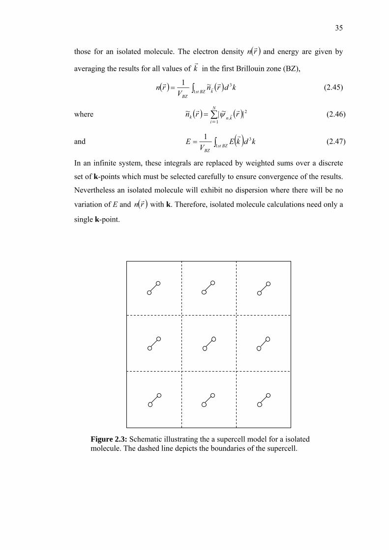
35
those for an isolated molecule. The electron density ( )rn r and energy are given by
averaging the results for all values of kr
in the first Brillouin zone (BZ),
( ) ( )∫=BZst k
BZ
kdrn~V
rn1
31 rrr (2.45)
where (2.46) ( ) ( )∑=
=N
ik,nk |r~|rn~
1
2rrrψ
and ( ) kdkEV
EBZst
BZ
31
1∫=
r (2.47)
In an infinite system, these integrals are replaced by weighted sums over a discrete
set of k-points which must be selected carefully to ensure convergence of the results.
Nevertheless an isolated molecule will exhibit no dispersion where there will be no
variation of E and ( )rn r with k. Therefore, isolated molecule calculations need only a
single k-point.
Figure 2.3: Schematic illustrating the a supercell model for a isolated molecule. The dashed line depicts the boundaries of the supercell.

36
Vpseudo
rrrc
( )rV r
r1 rc
rr
( )rrψ
pseudψ
All electronPseudo
Figure 2.4: Schematic representation of a psedopotential (left) and a pseudowavefunction (right) along with all-electron potential and wavefunction. The radius at which all-electron and pseudofunction values match and identical is rc. the pseudofunctions are smooth inside the core region.
3s
2s, 2p
“All Electron” free atom (AE)
1s = “Pseudo 3s”
Pseudo core
Constructred Pseudopotential (Pseudo)
Figure 2.5: Schematic depicting principle of pseudopotential, of which core electrons are neglected.

37
2.3.2 Projected Augmented Wave (PAW) –Pseudopotentials (PP) in Plane Wave Basis
Owing to the number of plane waves would exceed any practical limit and
lead to slow convergence, pseudopotentials (PP) instead of exact potentials need to
be applied. There are plenty of PP approximations such as norm-conserving PP (NC-
PP), ultrasoft PP (US-PP) and projected augmented wave (PAW) potentials. All
these three methods have a common that they are presently frozen core methods in
which the core electrons are pre-calculated in an atomic environment and kept frozen
in the course of the remaining calculations (see Figure 2.6). Among those, PAW
method which is developed by Blöch [57], is a very powerful tool for performing
electronic structure calculation within the framework of DFT, combining some of the
best features of PP and all-electron approaches [58]. In PAW, the all-electron wave
function is decomposed into three terms as depicted in Figure 3.7:
∑∑ +−= sitelm lmlm
sitelm lmlmk,nk,n cc~~
ε εεε εε φφψψ rr (2.48)
where k,nlmlm~p~c rψεε = (2.49)
where εlmp~ is the projector function, εφlm is the partial wave, lm is an index for the
angular and magnetic quantum numbers and ε refers to a particular reference energy.
The first term on the right side of equation (2.47) is the pseudowavefunction given
by equation (2.42) in PW expansion; the second term is the pseudowavefunction
represented on FFT-grid, on-site terms on atom-centered radial grids; while the third
term is the exact (or all-electron) onsite terms on radial grids. The decomposition is
also holds for charge density, kinetic energy, exchange-correlation energy and
Hartree energy. For instance, charge density ( )rn r can be represented by:
( ) ( ) ( ) ( )( ) ( ) ( )[ ] ( ) ( )[ ] ∑ ∑ +−=
+−=
k,n j,i,k,njijik,njik,nk,nk,nk,n rrr~r~~p~p~~fr~f
rnrn~rn~rn**
r rrrrrr
rrrrr
rrrr
φφφφψψψ2
11
(2.50)
where denotes the occupancy factor weighted by the fractional BZ
sampling volume, i = lmε, is the pseudo-density at one site, and is the
compensation density at site. Whilst kinetic energy can be represented by:
k,nf r
1n~ 1n

38
∑ ∑∑ ∑ ∑ Δ−+Δ−−Δ−=
+−=
siteji
)j,i(ji
k,n siteji
)j,i(jik,nk,nk,n
kin~~~~f
EE~E~E
φφρφφρψψr
rrr
11
(2.51)
where is an on-site density matrix. ∑=k,n
jik,nji ccf *r
rρ
= - +
AE (exact) Wavefunction
(WF)
Pseudo WF Pseudo onsite WF
AE onsite WF (compensation)
Exact potential (interstitial region) pseudopotential
Figure 2.6: Schematic depicting the decomposition of exact wavefunction (and energy) into three terms.
For KS orbitals expanded in a plane-wave basis set, atomic pseudopotentials
are employed, by which a local contribution and a angular momentum
dependent non-local contribution contributes to external energy or electron-
ion (ion = nucleus + core electrons) interaction energy, E
locE
nonlocE
ext which can be represented
by
nonloclocext EEE += (2.52)
with ( ) ( ) rdrnRrVE I
N
I
ionI,locloc
3
1
rrr−= ∑∫
= (2.53)
where is the local ionic pseudopotential with ionlocV IR
r is the Cartesian position of the
Ith ion, and local pseudopotential energy contains the electron-ion Coulomb
interaction.

CHAPTER 3
METHODOLOGY
In this research, VASP is used as the simulation tools for electronic structures of the
gallium arsenide clusters. Introduction and the calculation process of VASP are
discussed in this chapter.
3.1 Introduction to VASP
VASP which stands for Vienna Ab-Initio Software Package is initially
written by Mike Payne at MIT. It has the same roots as the CASTEP/CETEP code
but branched from this root at a very early stage [59]. The CASTEP version upon
which VASP is based only supported local pseudopotentials and a Car-Parrinello
type steepest descent algorithm. In 1989, VASP code had been brought by Jürgen
Hafner to Vienna, Austria and continued its development at the Institut für
Materialphysik of Universität Wien. The completion of the code had important
contribution from Jürgen Furthmüller who joined the group in Jan 1993 and Georg
Kresse who complete the parallelization in Jan 1997.
VASP is a versatile package for performing ab-initio quantum mechanical
molecular dynamics (MD) using pseudopotentials and a plane wave basis set. The

40
approach implemented in VASP is based on a finite-temperature LDA with the free
energy as variational quantity and an exact evaluation of instantaneous electronic
ground state at each MD-step. VASP uses efficient matrix diagonalization schemes
and an efficient Pulay/Broyden charge density mixing. All the problems occurring in
the original Car-Parrinello method based on the simultaneous integration of
electronic and ionic equations of motion, is avoided in these techniques. The
interaction between ions and electrons is described by ultra-soft Vanderbilt
pseudopotentials (US-PP) or by the projector-augmented wave (PAW) [57,60]
method, in which both of them allow for a considerable reduction of the number of
plane-waves per atom for transition metals and first row elements. Forces and stress
can be easily calculated with VASP and used to relax atoms into their instantaneous
ground state. Besides pure LDA for exchange-correlation functional, the gradient
corrected functionals that are implemented in VASP to account for non-locality in
exchange and correlation are: LM, PB, PW91, PBE, RPBE. Below is a short
summary of some highlights of the VASP code [59]:
a) Owing to use of PAW and US-PP method, the size of the basis-set can be
kept very small even for transition metal and first row elements like C and
O. Generally not more than 100 plane waves (PW) per atom are required to
describe bulk materials, in most cases even 50 PW per atom will be
sufficient for a reliable description.
b) In any PW program, the execution time scales like N3 for some parts of the
code, where N is the number of valence electrons in the system. In the
VASP, the pre-factors for the cubic parts are almost negligible leading to an
efficient scaling with respect to system size. This is possible by evaluating
the non-local contributions to the potentials in real space and by keeping the
number of orthogonalisations small. For system with roughly 2000
electronic bands, the N3 part becomes comparable to other parts. Therefore
we expect VASP to be useful for systems with up to 4000 valence electrons.
c) VASP uses a rather “traditional” and “old-fashioned” self-consistency cycle
to calculate the electronic ground state. The combination of this scheme
with efficient numerical methods leads to an efficient, robust and fast
scheme for evaluating the self-consistent solution of the Kohn-Sham
functional. The implemented iterative matrix diagonalisation schemes

41
(RMM-DIIS, and blocked Davidson) are probably among the fastest scheme
currently available.
d) VASP includes a full featured symmetry code which determines the
symmetry of arbitrary configurations automatically.
e) The symmetry code is also used to set up the Monkhorst Pack special points
(k-points) allowing an efficient calculation of bulk materials, symmetric
clusters. The integration of the band-structure energy over the Brillouin
zone is performed with smearing or tetrahedron methods. For the
tetrahedron method, Bloch corrections, which remove the quadratic error of
the linear tetrahedron method, can be used resulting in a fast convergence
speed with respect to the number of special points.
f) VASP runs equally well on super-scalar processors, vector computers and
parallel computers.
3.1.1 Software Packages Needed by VASP
VASP is a Fortran 90 program which is UNIX based. It requires a few
packages in order to successfully execute the simulation. The packages with brief
descriptions are listed as below:
i.) Fast Fourier Transform (FFT)
FFT is an efficient algorithm to compute the Discrete Fourier Transform and
its reverse. FFTs are of great importance to a wide variety of applications,
including solving partial differential equations and algorithms for quickly
multiplying integers. In multiplications involving complex numbers, it is
simply a method of laying out the computation which is much faster for large
values of N, where N is the number of samples in the sequence. FFT works by
using the divide and conquer approach, to break up the original N point
sample into two (N / 2) sequences in order to make a series of smaller
problem which is easier to be solved. For instance, FFTs approach only
require 1 multiplication and 2 additions by breaking it down into a series of 2

42
point samples of which the recombination of the points is minimal, whereas
the Discrete Fourier Transform needs (N-1)2 complex multiplication and N(N-
1) complex addition.
ii.) BLAS
Basic Linear Algebra Subprograms (BLAS) are routines that provide standard
building blocks for performing basic linear algebra operations such as vector
and matrix multiplication. The Level 1 BLAS perform scalar, vector and
vector-vector operations, the Level 2 BLAS perform matrix-vector operations,
and the Level 3 BLAS perform matrix-matrix operations. They are commonly
used in the development of high quality linear algebra software such as
LAPACK (Linear Algebra PACKage) owing to its efficiency, portability and
wide availability. Another package is ATLAS (Automatically Tuned Linear
Algebra Software) which can automatically generate optimized BLAS library.
It provides a full implementation of the BLAS application programming
interfaces (APIs) as well as some additional functions from LAPACK. In
addition, Intel Math Kernel Library (Intel® MKL) is also a package
comprised of BLAS and LAPACK which is specifically support Intel
processors.
iii.) MPI
For parallelization, VASP utilizes Message Passing Interface (MPI). Message
passing is a method by which data from one processor's memory is copied to
the memory of another processor. Hence, MPI is a language-independent
computer communications descriptive API, with defined semantics, and with
flexible interpretations. It was designed for high performance on both
massively parallel machines and on workstation clusters. Simply stated, the
goal of the MPI is to provide a widely used standard for writing message
passing programs with high performance or scalability and high portability.
MPICH (or MPICH2) and LAM/MPI are the examples of the implementation
of the MPI.

43
3.2 Files Used by VASP
Table 3.1 listed the input and out files used by VASP. Basically, four
important input files are INCAR, POTCAR, KPOINTS, and POSCAR, which are
indispensable in the execution of VASP.
Table 3.1: A relatively large number of input and output files of VASP.
File Input / Output File INCAR In
KPOINTS In POTCAR In POSCAR In
stout Out IBZKPT Out
CONTCAR Out CHGCAR In / Out
CHG Out OUTCAR Out
WAVECAR In / Out DOSCAR Out PCDAT Out
OSZICAR Out EIGENVAL Out TMPCAR In / Out
XDATCAR Out LOCPOT Out ELFCAR Out PROOUT Out PROCAR Out

44
3.2.1 INCAR File
INCAR is the central input file of VASP. It determines ‘what to do and how
to do it’, and contains a relatively large number of parameters. Most of these
parameters have convenient defaults and any of the default values should not be
changed without the awareness of their meaning. Some decisive parameters have to
be set for specific calculations for instances geometry optimization and local density
of states calculation. Therefore, understanding the parameters of INCAR helps
manipulating the desired calculation well.
3.2.2 POTCAR File
The POTCAR file contains the pseudopotential for each atomic species used
in the calculation. If the number of species is larger than one, simply combines the
POTCAR files of each species into one. The first pseudopotential will correspond to
the first species in the POSCAR and INCAR files, and so on. The POTCAR file also
contains information about the atoms like their mass, their valence, the energy of the
reference configuration for which the pseudopotential was created and others. In
addition, it also contains a default energy cutoff and therefore it is not necessary to
specify it in the INCAR file. The default value will be overwritten if a different value
is specified in INCAR file. There are two types of pseudopotentials supplied by
VASP, which are PAW and US-PP. Generally, the PAW potentials are more accurate
than the US-PP. There are two reasons for this: first, the radial cutoffs (core radii) are
smaller than the radii used for the US-PP, and second the PAW potentials reconstruct
the exact valence wavefunction with all nodes in the core region. Since the core radii
of the PAW potentials are smaller, the required energy cutoffs and basis sets are also
somewhat larger. Most of the PAW potentials were optimized to work at a cutoff of
250-300 eV. Pseudopotential that is used in this research is PAW for GGA (PBE).

45
3.2.3 POSCAR File
This file contains the lattice geometry and the ionic positions, optionally also
stating velocities and predictor-corrector coordinates for a Molecular Dynamic (MD)
run. After the lattice geometry, number of atom per atomic species is given in the
order consistent with the POTCAR and INCAR file. The atomic positions are
provided either in Cartesian coordinates or in direct coordinates which is respectively
fractional coordinates. In direct mode, the positions are given by
332211 axaxaxR rrrr++= , (3.1)
where are the three basis vectors and are the supplied values. In the
Cartesian mode the positions are scaled by a factor s, which is the lattice constant
used to scale all lattice vectors besides atomic coordinates, as given by:
31Kra 31Kx
⎟⎟⎟
⎠
⎞
⎜⎜⎜
⎝
⎛=
3
2
1
xxx
sRr
. (3.2)
In order to be recognized, “Cartesian” (or ‘C’, ‘c’, ‘K’ or ‘k’) is written before the
Cartesian atomic position, and any other character or “Direct” will switch to direct
mode.
3.2.4 KPOINTS File
The file KPOINTS must contain the k-point coordinates and weights or the
mesh size for creating the k-point grid. There are a few formats to create KPOINTS
file:
i.) Entering all k-points explicitly with Cartesian or reciprocal coordinates. In the
reciprocal mode, the k-points are given by
332211 bxbxbxkrrrr
++= , (3.3)

46
31K
rbwhere are the three reciprocal basis vector and are the supplied
value. In the Cartesian input format the k-points are given by:
31Kx
( 3212 x,x,xa
k )π=
r . (3.4)
Table 3.2 list the input required in order to specify the high symmetry k-points and
Figure 3.1 shows the example of important k point on the BZ of a face-centered
cubic (fcc) crystal.
k<111>
kz <001>
kx <100>
ky <010> Γ
ΣK W
Z X S
U
L
Q Λ
X
Figure 3.1: The First Brillouin zone of a fcc lattice, with high symmetry k-points and direction of planes marked. The zone center is Γ. Note that this is also the Wigner-Seitz cell of a body-centered cubic (bcc) lattice in real space.
Δ
Table 3.2: Coordinates of high symmetry k-points in Cartesian and reciprocal mode.
Point Cartesian coordinates (unit of 2π ) /a
Reciprocal coordinates ( ½ ¾ ¼ ) ( ½ 0 1 ) W
( ¾ ¾ 0 ) ( ⅜ ⅜ ¾ ) K
Γ ( 0 0 0 ) ( 0 0 0 ) ( ½ ½ ½ ) ( ½ ½ ½ ) L
( ½ ½ 0 ) X ( 0 0 1 )

47
ii.) Strings of k-points for bandstructure calculation that connecting specific
points of BZ, for example strings connecting Γ – X – W – Γ.
iii.) Automatic k-mesh generation which requires only the input of subdivisions
of the BZ in each direction and the origin for the k-mesh. The k-mesh is
generated according to the Monkhorst-Pack scheme [61]. This essentially
means that the sampling k-points are distributed homogeneously in the BZ,
with rows or columns of k-points running parallel to the reciprocal lattice
vectors that span the BZ. The construction rule of Monkhorst-Pack is
321 bububuk kjikji
rrrr++= (3.5)
ii
ii N,,,r,
NNr
u K212
12=
−−=where , (3.6)
31K
rb are the reciprocal lattice vectors, and Ni is the numbers of the
subdivisions that determines the number of k-points in i-direction. There are
two modes which are original Monkhorst-Pack, in which the k-mesh will be
shifted off Γ for even divisions to get a mesh which is centered symmetrically
around Γ, and Gamma mode which generates Monkhorst-Pack type meshes
with the origin being at the Γ point. All symmetry operations of Bravais
lattice are applied to all k-points and the irreducible k-points (or Irreducible
Brillouin Zone, IBZ) are then extracted.
3.3 Algorithm Used in VASP
Most of the algorithms implemented in VASP use an iterative matrix-
diagonalization scheme. The used algorithms are based on the conjugate gradient
scheme, block Davidson scheme, or a residual minimization scheme-direct inversion
and the iterative subspace (RMM-DIIS). An efficient Broyden/Pulay mixing scheme
is utilized for the mixing of the charge density. The typical flow-chart of VASP
calculating KS ground state is shown in Figure 3.2. Input charge-density and
wavefunctions
inn
bn N,,n, K1= φ , are independent quantities. At startup, charge-

48
density is by default taken as the superposition of atomic pseudo charge densities,
while wavefunctions by default is set up by filling wavefunction arrays with random
numbers. Within each self-consistency loop the charge density is used to set up the
Hamiltonian and the wavefunctions are then optimized iteratively so that they get
closer to the exact wavefunctions of this Hamiltonian. From the optimized
wavefunctions, a new charge density is calculated which is then mixed with the old
input-charge density. Figure 3.2 shows the flow chart of the algorithm and a more
detailed explanation is given in the next paragraph.
From the input charge densities, the local part of the Kohn-Sham Hamiltonian
( ) which is given by scnonloc
scloc VVTH ++=
[ ] [ ]inXCinHion
locsc
loc nnVVV μ++= (3.7)
and the corresponding double counting corrections
[ ] [ ] [ ] ( ) ( )∫−+−= rdrnrnEnEnE inXCinXCinHin.c.d3
21 rrμ (3.8)
are evaluated. For US-PP, the non-local part of the PP depends also on the local
potential and must be calculated accordingly. In the next step the Nb trial
wavefunctions are improved using iterative method and the new eigenenergies are
used to calculate a new Fermi energy and new partial occupancies. The total free
energy for the current iteration is calculated as the sum of the bandstructure energy,
the entropy term and double counting corrections (see equation 3.9).
[∑∑ +⎟⎠⎞
⎜⎝⎛ −
−=n
in.c.dn
nn
n nESfFσ
μεσε ] , (3.9)
where for occupied bands and 1=nf 0=nf for unoccupied bands, nε is
bandstructure energy, σ is a parameter to control the smearing of the occupation
function f ( )nfS, μ is the Fermi energy, and n is the entropy term. The calculated
energy conceptually corresponds to the energy evaluated from the Harris-Foulkes
functional, which is non-self-consistent (in contrast to the KS functional) and the
Harris Foulkes functional (defined in equation (3.9)) requires the calculation of the
bandstructure energy for a fixed charge density nin. In VASP, it is easy to evaluate
this energy by keeping the initial charge density fixed and iterating the eigenvectors
only until they are converged.

49
To obtain the exact KS-ground-state energy selfconsistency with respect to
the input charge density requires that the charge density residual vector given
by
[ innR ]
[ ] inoutin nnnR −= (3.10)
is zero, where the output charge density nout is calculated from the wavefunctions
with the relation of ( ) ( )∑=n
nnout rfrn 2rr φ . The residual vector allows
calculating a new charge density n
[ innR ]
in for the next selfconsistency loop. In principle it
is necessary to evaluate the eigenfunctions nφ exactly for each new input charge
density making nout and the residual vector R functionals of the input charge density
nin only. However, even in conjunction with complex Broyden like mixing
techniques, it turns out that this is not necessary if the final wavefunctions of the
previous mixing iteration are used as new initial trial wavefunctions. In such case a
few steps in the iterative matrix diagonalization are sufficient to obtain a reliable
result for the charge density residual vector R.
The conjugate gradient (CG) and the residual minimization (RMM) scheme
do not recalculate the exact KS eigenfunctions but an arbitrary linear combination of
the lowest eigenfunctions of a number of bands. Thus, it is in addition necessary to
diagonalize the Hamiltonian in the subspace spanned by the trial wavefunctions, and
to transform the wavefunctions accordingly as shown below.
kjkj
ikkjkji
jiij
U
UUH
H
φφ
ε
φφ
←
=
=H
(3.11)
This is called subspace diagonalization and can be performed either before or after
CG or RMM scheme, in which the first choice is preferable in the self-consistent
calculations.

50
Choose trial-charge nin and trial wavefunction nφ
Calculate Hartree potential [ ]inH nV and double counting corrections
Calculate XC potential [ ]inXC nV and double counting corrections
Set up non-local part scjiD
Sub-space diagonalization nnnn U φφ ′′ ⇐ (if required)
Iterative improvement of nn ,εφ
Gram-Schmidt orthogonalizatoin (if required)
New partial occupancies fn
Free energy ( ) [ ]∑∑ +−=n
in.c.dnnn
n nEfSfF σε
New charge density nout from wavefunctions
Mixing of charge density nin, nout ⇒ new nin
breakEE >Δno
Figure 3.2: Flow chart of iterative methods for the diagonalization of the KS-Hamiltonian in conjunction with an iterative improvement (mixing techniques) of the charge density for the calculation of KS-ground-state.
Calculate force, update ions

51
Gram-Schmidt is a orthogonalization method which is only required for the RMM
scheme and it is performed after the scheme. In general all iterative algorithms work
very similar, where the core quantity is the residual vector:
( ) nnnnnn ,R φφεφε HH =−= (3.12)
The residual vector is added to the wavefunction nφ , and the algorithms differ in the
way this is exactly done.
3.3.1 Conjugate Gradient Algorithm
The conjugate gradient algorithm selects the successive direction vectors as a
conjugate version of the successive gradients obtained as the method progresses.
Thus, the directions are not specified beforehand, but rather are determined
sequentially at each step of the iteration. At step k one evaluates the current negative
gradient vector and adds to it a linear combination of the previous direction vectors
to obtain a new conjugate direction vector along which to move. There are three
primary advantages to this method of direction selection. First, unless the solution is
attained in less than n steps, the gradient is always nonzero and linearly independent
of all previous direction vectors. Indeed, as the corollary states, the gradient is
orthogonal to the subspace
kg
kβ generated by d , d , …..,dk+10 1 . If the solution is
reached before n steps are taken, the gradient vanishes and the process terminates.
Second, a more important advantage of the conjugate gradient method is the
especially simple formula that is used to determine the new direction vector. This
simplicity makes the method only slightly more complicated than steepest descent.
Third, because the directions are based on the gradients, the process makes good
uniform progress toward the solution at every step. This is in contrast to the situation
for arbitrary sequences of conjugate directions in which progress may be slight until

52
the final few steps. Although for the pure quadratic problem uniform progress is of
no great importance, it is important for generalizations to non quadratic problems.
n
kkkk
kTk
kTk
kgk
kkkk
kTk
kTk
k
xdgd
QddQdg
k
bQxdxx
Qdddgnk
gdbQxg
β
β
α
α
+−←
←
+←+←
−←
−=−←
+←
++
+
++
+
11
1
11
1
00
00
1,........,0
1.2.
Step 3b when k = 0 is a steepest descent. Each subsequent step moves in a
direction that modifies the opposite of the current gradient by a factor of the previous
direction. Step 3a – 3e gives us the Q-orthogonality of the descent vector
. 10 ,......., −ndd
3.3.2 Block Davidson Algorithms
Davidson [59] has devised methods that are now widely applied to electronic
structure problems. There are a number of variations that cannot be covered here. A
primary point is that the Davidson approach is closely related to the Lanczos
algorithm, but adapted to be more efficient for problems in which the operator is
diagonally dominant. This is often the case in electronic structure problems for
example plane wave algorithms.
3. for do
a)
b)c)
d)
e)4. return.

53
The flavor of the Davidson methods can be illustrated by defining the
diagonal part of the Hamiltonian matrix as '' mmmmmm HD δ= and rewriting the
eigenvalue problem as εψψ =H
( ) ( )ψεψ DIDH −=− (3.13)
or ( ) ( )ψεψ DHDI −−= −1 (3.14)
Here I is the unit matrix, inversion of I – D is trivial, and H – D involves only
off-diagonal elements. The latter equation is very similar to perturbation theory and
suggests iterative procedures that converge rapidly if the diagonal part of the
Hamiltonian is dominant. An algorithm has been suggested by Lenthe and Pulay [91]
that involves three vectors at each step of the iteration.
3.3.3 Residual Minimization Scheme-Direct Inversion In The Iterative
Subspace (RMM-DIIS)
The approaches described up to now (and the minimization methods
described below) converge to the lowest state with no problems because the ground
state is an absolute minimum. In order to find higher states, they must ensure
orthogonality, either implicitly as in the Lanczos methods or by explicit
orthogonalization. The residual minimization method (RMM) proposed by Pulay [92]
avoids this requirement and converges to the state in the spectrum with eigenvalue
closest to the trial eigenvalue ε because it minimizes the norm of a “residual vector”
instead of the energy.

54
Since the approach of Pulay minimizes the residual in the full Krylov
iterative space generated by previous iterations, the method is known as RMM-DIIS
for “residual minimization method by direct inversion in the iterative subspace”. The
general idea is
∑+
=
+ +=1
1
1n
j
jj
oo
n cc δψψψ (3.15)
1+nRwhere the entire set of is chosen to minimize the norm of the residual jc . (Pre-
conditioning can also be applied at each step [57] to speed the convergence). The coefficients can be obtained by diagonalizing the Hamiltonian in the iterative
subspace jc
( )no ψψψψ ..........,, 21 , which is a miniscule operation since the number of vectors is at most 10 or so. The time-consuming step is the operation ψΗ , which is a matrix operation requiring, in general, ( )2
bNO operations for each eigenvector ψ , where is the size of the basis. bN
3.4 Simulation Process
Generally, the simulation process in this research contains the steps shown in
Figure 3.3 and this flow chart is applied to all of the structures in order to obtain the
electronic structures. Each step of the process will be discussed in the next sections.
The discussion of the methods provided in the following is not specific to any of the
simulated structures but is universal and generally discussed.

55
Construct the cluster
Geometry optimization on the cluster
Density of states and Bandstructures calculation on the optimized cluster
Energy, density of states and bandstructures are obtained
Figure 3.3: Flow chart of the electronic structure simulation process of gallium arsenide
clusters.
3.4.1 Construction of the Clusters
Construction of a structure is done by specifying the Cartesian or direct
coordinate of each atom of the structure in the POSCAR file. As discussed in the
Section 2.2.1, due to the boundary conditions in VASP which are periodic in all three
dimensions, supercell method is used for isolated structure calculations. The
supercell is a simple cubic cell with large lattice length in order to create sufficient
vacuum region for the isolated structure. The purpose is to eliminate the interaction
between isolated clusters across the cell boundary in the periodic array and to make
sure the results will be those for the isolated cluster. The structure of the cluster is
built in the middle of the supercell. The supercell size is at least three times larger
than the lattice constant of solid gallium arsenide. The distance between two isolated
clusters is made about 2-3 times the size of the clusters to make sure the
intermolecular interaction is negligible. In this research, the minimum lattice length
of the supercell is taken to be 17 Å for the smallest clusters as three to six atoms
clusters. Example is shown below with gallium arsenide cluster of 4 atoms. The

56
largest distance between atoms is taken (2.816 Å) and lattice length of 17 Å is built
so that the distance between clusters is more than 10 Å, which is more than 3 times
the individual cluster size. The lattice length increases as the number of atom of the
cluster increases.
(a) (b)
Figure 3.4: (a) Bulk gallium arsenide with its unit cells repeated in 3 dimensions. (b) supercells with Ga2As2 cluster in the center and the distance between clusters is large. The show the Ga atoms and show the As atoms.
3.4.2 Geometry Optimization
Geometry optimization is used to find the minima on the potential energy
surface with these minimum energy structures representing equilibrium structures.
When we first construct a raw cluster structure, the ion positions and bond lengths
are not accurate and the structure is not in a stable condition. Thus geometry
optimization is needed to be accomplished before any other calculation of the
relevant structure. Force is a crucial element in the geometry optimization and it is
relatively simple to be calculated by using plane wave basis set. The forces on a
nucleus I with position RI can be conveniently described as II RFrr
∂∂=F , which
contains Pulay as well as Hellmann-Feymann contributions as shown in equation
(2.40). F is the free energy which depends on the wavefunction nφ , the partial
occupancies fn, expansion coefficients Cnq and the ionic position RI. This force can

57
then be used to find the ground state position of the atoms. The forces can be used to
calculate a molecular dynamics trajectory. As the atoms move to new position, the
electronic wavefunctions must also change. As the forces point to the minimum in
the energy variation where the forces vanish, the atoms move toward an equilibrium
structure. Thus, geometry optimization is also referred to as energy minimization.
In VASP, geometry optimization can be done with a few algorithms such as
standard ab-initio molecular dynamics (MD), RMM-DIIS implementation of quasi-
Newton, conjugate gradient (CG) and damped molecular dynamics. MD is a
algorithm that performs the energy minimization into global minimum whereas all
other algorithms are destined for relaxations into a local energy minimum. Damped
MD is often useful for very bad initial guess structure while RMM-DIIS is usually
the best choice that is close to the local minimum but fails badly if the initial
positions are a bad guess. Therefore for difficult relaxation problems, CG is
recommended because it possesses the most reliable backup routines.
In this research, the geometry of the clusters has been determined by static
relaxation using CG minimization and exact Hellmann-Feynman forces. For small
clusters (n = 2 – 6), the most stable geometry is found from the many possible
configurations with varying coordinates. When the size of the clusters is getting
larger, the number of topologically distinct structures which is called isomers
increases very rapidly with the number of atoms, n. Therefore, for larger clusters
(n > 6) dynamical simulated annealing (SA) of the cluster structure was performed in
addition. SA runs can be very helpful for an automatic determination of favorable
structural models and it can avoid unfavorable local minima in the energy surface.
The elevated temperatures strategy used in SA allows an efficient sampling of the
potential energy surface [62]. Final structural refinement using the static CG
approach for local minimization is performed after the system is cooled down to the
best configurations. The following sections describe the parameters for CG and SA
algorithms in the INCAR file.

58
SA CG Stable geometry
Figure 3.5: Algorithm of geometry optimization used for large clusters.
3.4.2.1 INCAR for Conjugate Gradient Geometry Optimization
Other than the default parameters specified in the POTCAR file, the
following parameters is written in the INCAR file to overwrite those in the POTCAR
(see Figure 3.6). Phrases after “!” briefly describe the flags respectively. The key of
switching to CG algorithm is by setting IBRION = 2 and POTIM = 0.1 determine the
scaling constant for the forces. The simulation is started with wavefunctions
initialized according to flag INIWAV (default = 1 :fill wavefunction array with
random numbers) and superposition of atomic charge densities is taken with
ICHARGE = 2. High energy cutoff and precision are set to ensure the accuracy of
the results. For cluster or isolated molecule with large supercell, Gaussian smearing
is adopted and the width of the smearing is set to a significantly small value, of
which 0.001 is set in this research. During the geometry optimization, the shape and
volume of the supercell is kept constant and only the internal ions are relaxed
(ISIF = 2), in the meanwhile force and stress tensor are calculated. The total energies
and equilibrium geometries will converge to within the chosen precision (EDIFF and
EDIFFG). EDIFF specifies the global break condition for the electronic self-
consistency loop. The relaxation of the electronic degrees of freedom will be stopped
if the total or free energy and the eigenvalues change between two steps are both
smaller than EDIFF. Whereas EDIFFG defines the break conditions for the ionic
relaxation loop. For negative value, the relaxation will stop if all forces are smaller
than | EDIFFG | (in unit of eV/Å). Sixty numbers of ionic steps is set and more steps
should be added if convergence can not be reached.

59
SYSTEM = Gallium arsenide cluster ## Start parameter for this Run: ISTART = 0 ! job : 0-new 1-cont 2-samecut ICHARGE = 2 ! charge: 1-file 2-atom 10-const PREC = HIGH ## Electronic Relaxation ENCUT = 350 eV EDIFF = 0.1E-0.7 ! stopping-criterion for ELM ## Ionic Relaxation IBRION = 2 ! ionic relax: 0-MD 1-qausi-New 2-CG ISIF = 2 ! stress and relaxation
EDIFFG = -0.01 ! stopping-criterion for IOM NSW = 60 ! number of steps for IOM POTIM = 0.1 ! time-step for ionic-motion
## DOS related values ISMEAR = 0 ! -4-tet -1-fermi 0-gaussian SIGMA = 0.001 ! broadening in eV
Figure 3.6: Parameters for CG algorithm in INCAR file.
In the first step of CG algorithm, ions are changed along the direction of the
steepest descent which is the direction of the calculated forces and stress tensor. The
CG method requires a line minimization which is performed in several steps as
below:
1. First a trial step into the search direction (scaled gradients) is done with the
length of the trial step controlled by the POTIM parameter. Then the energy
and the forces are recalculated.
2. The approximate minimum of the total energy is calculated from a cubic or
1xr0xr quadratic interpolation using energies and forces at and (see Figure
3.7), taking into account the change of the total energy and the change of the
forces, then a corrector step to the approximate minimum is performed.
3. After the corrector step the forces and energy are recalculated and it is
checked whether the forces contain a significant component parallel to the

60
previous search direction. If this is the case, the line minimization is
improved by further corrector steps using a variant of Brent’s algorithms.
3.4.2.2 INCAR for Simulate Annealing
Simulated annealing (SA) is a generic probabilistic meta-algorithm for the
global optimization problem for locating a good approximation to the global
optimum of a given function in a large search space. It is a generalization of a Monte
Carlo method for examining the equations of state and frozen states of n-body
systems [63]. This technique involves heating and controlled cooling of a material to
increase the size of its crystals and reduce their defects. The heat causes the atoms to
become loose from their initial positions and wander randomly through states of
higher energy whereas the slow cooling provides more chances of finding
configurations with lower internal energy than the initial one. SA's major advantage
over other methods is an ability to avoid becoming trapped at local minima.
x0
x1
xtrial 2
xtrial 1
Figure 3.7: Conjugate gradient techniques: (top) Steepest descent step from 0x
x0
0gr x1
r
search for minimum along 0gr by performing several trial steps to 1xr . (below) New gradient ( )10 xgg rrr
= is determined and 1sr (green arrow) is conjugated. For 2D functions the gradient now points directly to the minimum. Minimization along search direction 1sr is continued.
x0
x2
1gr
s1x1

61
Because of the SA is a dynamic process that involves temperatures, there are
a few parameters are to be included in the INCAR file as shown in Figure 4.8.
SYSTEM = Gallium arsenide cluster ## Start parameter for this Run: ISTART = 0 ! job : 0-new 1-cont 2-samecut ICHARGE = 2 ! charge: 1-file 2-atom 10-const ## Electronic Relaxation ENCUT = 350 eV IALGO = 48 ! RMM-DIIS algorithm for electrons
LREAL = .FALSE ! evaluate projection operators in rec. space NELMIN = 4 ! do a minimum of four electronic steps MAXMIX = 50 ! keep dielectric function btwn ionic movement
## Ionic Relaxation
IBRION = 0 ! ionic relax: 0-MD 1-qausi-New 2-CG NSW = 600 ! number of steps for IOM POTIM = 3.00 ! time-step for ionic-motion NBLOCK = 1 ! inner block SMASS = -1.00 ! Nose mass-parameter (am) TEBEG = 1700 ! temperature TEEND = 0
Figure 3.8: Parameters for SA algorithm in INCAR file.
Same as CG process, the energy cutoff of 350eV is used in the SA algorithm.
IBRION = 0 denotes that the MD algorithm is combined in the SA process. RMM-
DIIS algorithm is set for electrons in order to reduce the number of
orthonormalization steps and speed up the calculation. The projection operators are
evaluated in reciprocal space (LREAL = FALSE) and at least 4 electronic iterations
per ionic step is required for MD runs. MAXMIX specifies the maximum number of
vectors stored in the Broyden/Pulay mixer or in other words it corresponds to the
maximal rank of the approximation of the charge dielectric function build up by the
mixer. It should be set roughly three times the number of iterations in the first ionic
step. In the process of simulated annealing, the initial temperature is set to a very
high temperature. This temperature is set to 1700 K which is a bit higher than the
62
melting point of gallium arsenide (1511 K). While these are indeed indicators of a
transition from solid to liquid, the temperature at which this happen in a MD
simulation is invariably higher than the melting temperature. In fact, the melting
point is by definition the temperature at which the solid and the liquid phase coexist
(they have the same free energy). However, lacking a liquid seed from where the
liquid could nucleate and grow, overheating above melting commonly occurs. In this
region the system is in a thermodynamically metastable state, nevertheless it appears
stable within the simulation time. An overheated bulk crystal breaks down when its
mechanical instability point is reached. This point may correspond to the vanishing
of one of the shear moduli of the material or to similar instabilities, and is typically
larger than melting temperature by an amount of the order of 20-30%. If the initial
annealing temperature is too low, the search space is limited and the search becomes
trapped in a local region. If the initial temperature is too high, the algorithm spends a
lot of time “boiling around” and wasting CPU time. The idea is to initially have a
high percentage of moves that are accepted.
The temperature reaches zero at the end after 600 numbers of ionic steps. 3 fs
time step is set for the ionic motion. The decrement of the temperature is controlled
by the option SMASS. In this case the velocities of the MD are scaled by each
NBLOCK step to the temperature produced from the formalism TEMP = TEBEG +
(TEEND – TEBEG) × NSTEP / NSW, where NSTEP is the current step (starting
from 1).
Figure 3.9 is the flowchart illustrating the algorithm of SA. There are two
major processes that take place in the simulated annealing algorithm. First, for each
temperature, the simulated annealing algorithm runs through a number of cycles. The
number of cycles is predetermined by the programmer. As a cycle runs, the inputs
are randomized. The randomization process takes the previous input values and the
current temperature as inputs. The input values are then randomized according to the
temperature. A higher temperature will result in more randomization; a lower
temperature will result in less randomization.

63
Once the specified number of training cycles have been completed, the
temperature can be lowered. Once the temperature is lowered, it is determined
whether or not the temperature has reached the lowest temperature allowed. If the
temperature is not lower than the lowest temperature allowed, then the temperature is
lowered and another cycle of randomizations will take place. If the temperature is
lower than the lowest temperature allowed, the simulated annealing algorithm
terminates.
At the core of the simulated annealing algorithm is the randomization of the
input values. This randomization is ultimately what causes simulated annealing to
alter the input values that the algorithm is seeking to minimize. The randomization
process must often be customized for different problems.
By analogy with this physical process, each step of the SA algorithm replaces
the current solution by a random "nearby" solution, chosen with a probability that
depends on the difference between the corresponding function values and on a global
parameter, which is temperature that gradually decreases during the process. The
dependency is such that the current solution changes almost randomly when the
temperature is large, but increasingly move downhill to lower kinetic energy as the
temperature goes to zero. This optimization process does not only proceed uniformly
downhill, but is allowed to make occasional uphill moves. The allowance for moving
uphill saves the method from becoming stuck at local minima.

64
Start
Randomize according to the current temperature
Better than current
solution?
Reached max tries for this temperature?
Decrease temperature by specified rate
Reached specified lowest
temperature?
Replace current solution with randomized
solution
Yes
No
No
No
Yes
YesStop
Figure 3.9: Flowchart illustrating the algorithm of SA.

65
3.4.2.3 KPOINTS for Geometry Optimization
As discussed in section 2.2.1, only single k-point is needed for isolated
molecule. Therefore, gamma point is used for the geometry optimization of the
isolated clusters in this research and the KPOINTS file for such case is shown in
Figure 3.10.
Monkhorst Pack ! comment 0 ! Automatic generation Monkhorst Pack ! M=Monkhorst-Pack
1 1 1 ! grid 0 0 0 ! shift
Figure 3.10: Parameters for geometry optimization in KPOINTS file.
The KPOINTS file is written in the Monkhorst-Pack scheme as discussed in
the section 3.2.4. The automatic generated k-mesh will be created and given in the
file IBZKPT. The fourth line of the KPOINTS gives a gamma point with the
coordinate (0 0 0) and the weight 1.0.
3.4.3 Electronic Structures Calculations
After the geometry optimization is performed and the stable geometry is
obtained, electronic structure calculations are then done by using the final structure
generated. The usual way to calculate DOS and bandstructure is the following: first
charge density using a few k-points (gamma point for the case of isolated clusters) in
a static self-consistent run is performed; the next step is to perform a non-
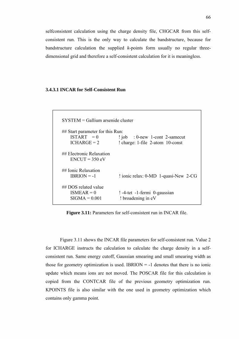
66
selfconsistent calculation using the charge density file, CHGCAR from this self-
consistent run. This is the only way to calculate the bandstructure, because for
bandstructure calculation the supplied k-points form usually no regular three-
dimensional grid and therefore a self-consistent calculation for it is meaningless.
3.4.3.1 INCAR for Self-Consistent Run
SYSTEM = Gallium arsenide cluster ## Start parameter for this Run: ISTART = 0 ! job : 0-new 1-cont 2-samecut ICHARGE = 2 ! charge: 1-file 2-atom 10-const ## Electronic Relaxation ENCUT = 350 eV
## Ionic Relaxation IBRION = -1 ! ionic relax: 0-MD 1-quasi-New 2-CG ## DOS related value ISMEAR = 0 ! -4-tet -1-fermi 0-gaussian SIGMA = 0.001 ! broadening in eV
Figure 3.11: Parameters for self-consistent run in INCAR file.
Figure 3.11 shows the INCAR file parameters for self-consistent run. Value 2
for ICHARGE instructs the calculation to calculate the charge density in a self-
consistent run. Same energy cutoff, Gaussian smearing and small smearing width as
those for geometry optimization is used. IBRION = -1 denotes that there is no ionic
update which means ions are not moved. The POSCAR file for this calculation is
copied from the CONTCAR file of the previous geometry optimization run.
KPOINTS file is also similar with the one used in geometry optimization which
contains only gamma point.
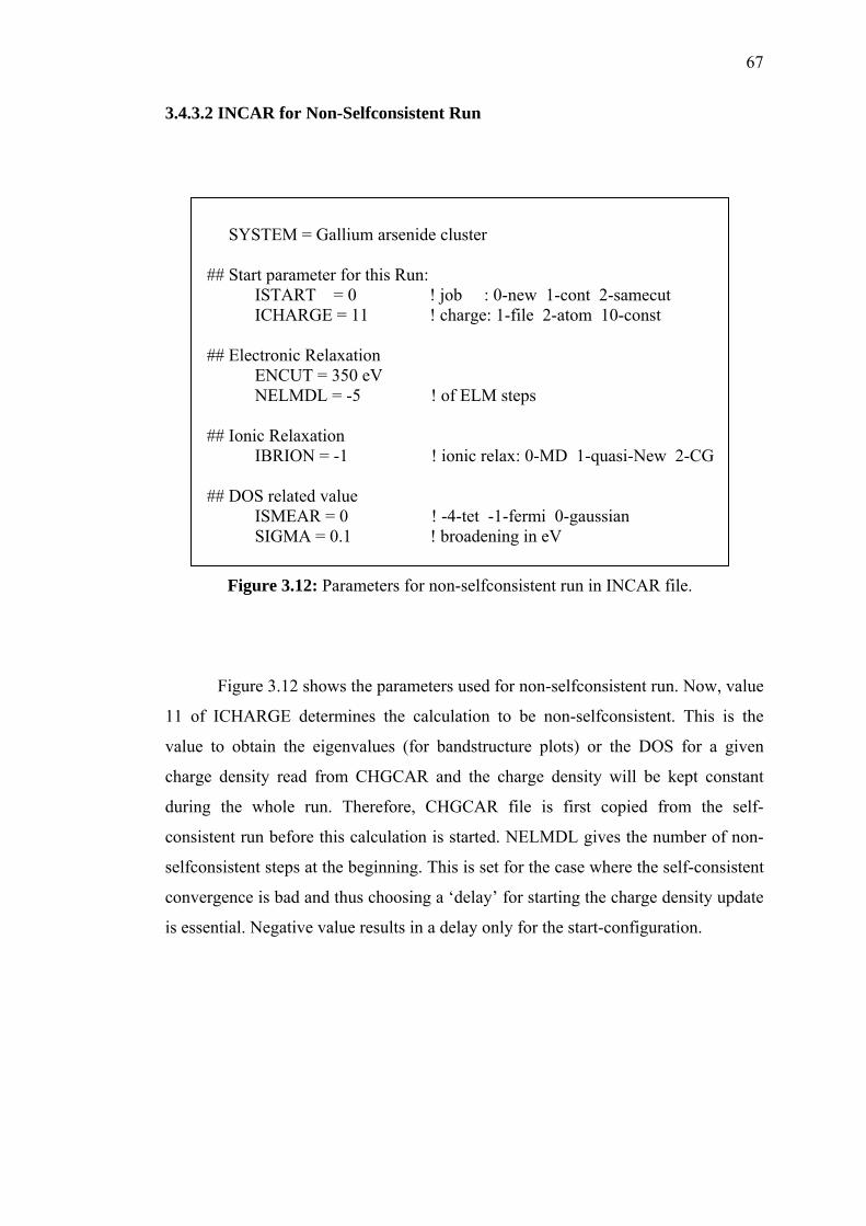
67
3.4.3.2 INCAR for Non-Selfconsistent Run
SYSTEM = Gallium arsenide cluster ## Start parameter for this Run: ISTART = 0 ! job : 0-new 1-cont 2-samecut ICHARGE = 11 ! charge: 1-file 2-atom 10-const ## Electronic Relaxation ENCUT = 350 eV NELMDL = -5 ! of ELM steps
## Ionic Relaxation IBRION = -1 ! ionic relax: 0-MD 1-quasi-New 2-CG ## DOS related value ISMEAR = 0 ! -4-tet -1-fermi 0-gaussian SIGMA = 0.1 ! broadening in eV
Figure 3.12: Parameters for non-selfconsistent run in INCAR file.
Figure 3.12 shows the parameters used for non-selfconsistent run. Now, value
11 of ICHARGE determines the calculation to be non-selfconsistent. This is the
value to obtain the eigenvalues (for bandstructure plots) or the DOS for a given
charge density read from CHGCAR and the charge density will be kept constant
during the whole run. Therefore, CHGCAR file is first copied from the self-
consistent run before this calculation is started. NELMDL gives the number of non-
selfconsistent steps at the beginning. This is set for the case where the self-consistent
convergence is bad and thus choosing a ‘delay’ for starting the charge density update
is essential. Negative value results in a delay only for the start-configuration.

68
3.4.3.3 KPOINTS for Non-selfconsistent and Bandstructure
The k-points used for bandstructrue is different from the previous run and its
KPOINTS file contains strings of k-points as shown in Figure 3.13.
k-points for bandstructure L-G-X-U K-G 10 ! 10 intersections Line-mode Reciprocal 0.500 0.500 0.500 ! L 0.000 0.000 0.000 ! gamma 0.000 0.000 0.000 ! gamma 0.000 0.500 0.500 ! X 0.000 0.500 0.500 ! X 0.250 0.625 0.625 ! U 0.375 0.750 0.375 ! K 0.000 0.000 0.000 ! gamma
Figure 3.13: Parameters for non-selfconsistent run in KPOINTS file.
The strings of k-points connect the specific points of L-G-X-U and K-G of
the Brillouin zone (refer Figure 3.1). The coordinates of the k-points are given in
reciprocal mode. Value 10 in the second line instructs VASP to generate 10 k-points
between the first and second supplied points, 10 k-points between the third and the
fourth, and so on. The bandstructure is then plotted according to these specific k-
points.

CHAPTER 4
RESULTS AND DISCUSSION
4.1 Simulation of Bulk Gallium Arsenide and Gallium Arsenide Dimer
As a first step, bulk gallium arsenide is calculated by using VASP for the
purpose of comparison with the clusters as well as for accuracy assurance. In
addition, dimmer is an excellent test system. If a pseudopotential has passed dimer
and bulk calculation, one can be quite confident that the pseudopotential posseses
excellent transferability. Bulk gallium arsenide is constructed according to its zinc
blende structure that is in F43m space group, which follows face-centered-cubic (fcc)
bravais lattice.
The geometry optimization gives the structure with lattice constant 5.632 Å.
This is close to the experimental lattice constant 5.653 Å [64]. For Ga1As1 dimer, the
approach is same as those for the clusters, which is using supercell method. The
result shows the bond length of the Ga1As1 is 2.580 Å, which is also in good
agreement to the experimental results of 2.53 Å ± 0.02 Å [12]. Density of state

70
(DOS) and bandstructure is further calculated for bulk gallium arsenide. The DOS
and bandstructure are corresponding to each other and from both graph, the obtained
bandgap value (direct bandgap) is 0.354 eV. This is lower than the experimental
value 1.424 eV. It has been claimed that the reason lies the ground state emphasis of
DFT and thus it underestimated the bandgap value [65]. The presence of a
discontinuity in the true DFT exchange-correlation functional derivative is also the
reason leading to the bandgap underestimation.
Figure 4.1: Structure of zinc blende bulk GaAs (Left). Structure of Ga1As1 dimer (Right).

71
zinc blende, GaAs
(ii)
Energy (eV)
Bandstructure
zinc blende, GaAs
K-point distances
a
b
Figure 4.2: Bandstructure of bulk GaAs. Point a represents highest energy of valence band (band or area below a) while point b represents the lowestenergy of the conduction band (band or area after b). Both bandstructure and DOS are corresponding to each other.

72
ba
Figure 4.3: DOS of bulk GaAs. Point a represents highest energy of valence band (band or area below a) while point b represents the lowest energy of the conduction band (band or area after b). Both bandstructure and DOS are corresponding to each other.

73
4.2 The Effect of Size on the Electronic Structures of Gallium Arsenide
Clusters
In order to compare the results for variable size, the gallium arsenide clusters
are simulated by clusters with different number of gallium arsenide atom. The size
would rather to be termed as the number of atoms. A bare cluster has a large number
of dangling bonds on its surface, which shows strong chemical reactivity and induces
an unstable condition for the cluster.
During the geometry optimization, the surface will reconstruct and eliminate
dangling bonds to minimize the surface potential and consequently lead to a stable
structure. Therefore, in order to maintain the regular tetrahedron bonding
configuration, the cluster is terminated or passivated by hydrogen. With the presence
of hydrogen atoms on the dangling bonds of the clusters, the surface tension is
significantly reduced and thus has a function of stabilization.
The clusters were built from arrangement corresponding to the bulk gallium
arsenide fragment. Geometry optimization was performed with conjugate gradient
process and only internal parameters (atoms’ position and distance) change without
fluctuation of the supercell’s size. Four hydrogenated gallium arsenide clusters were
compared, which are Ga4As4H12, Ga5As6H16, Ga7As6H16 and Ga7As6H19.

74
Ga4As4H12
Ga7As6H19Ga7As6H16
Ga5As6H16
Figure 4.4: Ball and stick for hydrogenated gallium arsenide clusters, GaxAsyHz

75
Ga4As4H12
Ga5As6H16

76
Ga7As6H16
Ga7As6H19
Figure 4.5: Bandstructure and DOS of hydrogenated gallium arsenide clusters, GaxAsyHz.

77
The following list the bandgap energy of each cluster obtained from the
bandstructures in Figure 4.5.
Table 4.1: Bandgap energy for each of the cluster. Values in the brackets are the bandgap (eV) from Asok K. Ray et.al [87].
Total Number Of
Atoms In The
Clusters
GaxAsyHz
HOMO (eV) LUMO (eV) Bandgap (eV)
20 Ga4As4H12 -8.20 -0.86 7.34 (7.462) 27 Ga5As6H16 -6.01 -1.59 4.42 (4.584) 29 Ga7As6H16 -5.23 -1.65 3.58 (3.698) 32 Ga7As6H19 -3.89 -1.97 1.92 (2.057)
HOMO-LUMO Energy Levels in GaAs Clusters
-9-8-7-6-5-4-3-2-10
0 5 10 15 20 25 30 35
Total Number Of Atoms In The Clusters
Ene
rgy
(eV
)
HOMO
LUMO
Figure 4.6: Band shift related to the cluster size. The upper line is HOMO energy value while lower line is LUMO energy value.
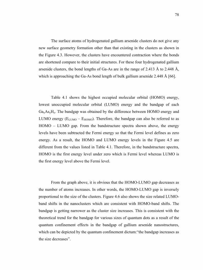
78
The surface atoms of hydrogenated gallium arsenide clusters do not give any
new surface geometry formation other than that existing in the clusters as shown in
the Figure 4.3. However, the clusters have encountered contraction where the bonds
are shortened compare to their initial structures. For these four hydrogenated gallium
arsenide clusters, the bond lengths of Ga-As are in the range of 2.413 Å to 2.448 Å,
which is approaching the Ga-As bond length of bulk gallium arsenide 2.448 Å [66].
Table 4.1 shows the highest occupied molecular orbital (HOMO) energy,
lowest unoccupied molecular orbital (LUMO) energy and the bandgap of each
GaxAsyHz. The bandgap was obtained by the difference between HOMO energy and
LUMO energy (ELUMO – EHOMO). Therefore, the bandgap can also be referred to as
HOMO – LUMO gap. From the bandstructure spectra shown above, the energy
levels have been subtracted the Fermi energy so that the Fermi level defines as zero
energy. As a result, the HOMO and LUMO energy levels in the Figure 4.5 are
different from the values listed in Table 4.1. Therefore, in the bandstructure spectra,
HOMO is the first energy level under zero which is Fermi level whereas LUMO is
the first energy level above the Fermi level.
From the graph above, it is obvious that the HOMO-LUMO gap decreases as
the number of atoms increases. In other words, the HOMO-LUMO gap is inversely
proportional to the size of the clusters. Figure 4.6 also shows the size related LUMO-
band shifts in the nanoclusters which are consistent with HOMO-band shifts. The
bandgap is getting narrower as the cluster size increases. This is consistent with the
theoretical trend for the bandgap for various sizes of quantum dots as a result of the
quantum confinement effects in the bandgap of gallium arsenide nanostructures,
which can be depicted by the quantum confinement dictum:“the bandgap increases as
the size decreases”.
79
The HOMO-LUMO band-shift results in the red-shifting of the bandgap.
From Figure 4.5, it is clear that the correlation between the bandgap and the number
of atom is not linear. This indicates that the bandgap also depends on other factors
which among them are the symmetry of the cluster and the specific transition
involved. The important implication of Figure 4.6 is the relation between the cluster
size and the bandgap as discussed above. Theoretical bandgaps of the four clusters
(Ga4As4H12, Ga5As6H16, Ga7As6H16 and Ga7As6H19) are shown in the bracket in
Table 4.1. As discussed earlier, the calculated bandgaps are underestimated
compared to the theoretical data.
In comparison, it is obvious that the bandgap for each of the cluster is much
larger than the bandgap of bulk gallium arsenide since cluster is much smaller than
the bohr radius of bulk gallium arsenide is 12nm [67]. For bulk gallium arsenide,
there are optical activities due to direct bandgap.
Therefore, for hydrogenated gallium arsenide cluster, the light emission can
be controlled by altering the size of the cluster which results in different color of
light. As a result, it can be observed that the DOS of cluster is different from the one
of bulk. The DOS is not continuous but is in discrete form.
Hence, it is referred to as discrete energy spectrum instead of DOS. In
conjunction with the DOS changing, bandstructure has also become a straight
vertical line in consistent with the discrete spectrum, which is a result of single-point
calculation. Although the calculated values are not in good agreement with the
experimental values (since bandgap is underestimated by DFT), the results show
80
qualitative trends and relativity of the electronic properties of gallium arsenide
nanostructures.
4.3 The Effect of Shape on the Electronic Structures of Gallium Arsenide
Clusters
In this section, the shape effect to the electronic structures of gallium arsenide
clusters is discussed. Unlike the hydrogenated gallium arsenide clusters studied
previously, gallium arsenide clusters used for the study of shape effect are bare
clusters without any passivation with other elements.
After the energy minimization algorithm; conjugate gradient (CG) and
simulated annealing (SA) the ground state structures for GaxAsy (x+y≤15) as shown
in Figure 4.7 were obtained. From an overall view, it could be observed that the
structures of the optimized bare gallium arsenide clusters are different from each
other and they have their own geometries. These optimized geometrical structures
will be discussed in the next section and the discussion of electronic structures will
be made next.

81
Ga1As2 Ga2As2 Ga2As3 Ga3As3
Ga3As4 Ga4As4 Ga4As5
Ga5As5 Ga5As6 Ga6As6
Ga7As6 Ga7As7 Ga7As8
Figure 4.7 : Lowest energy geometries for the GaxAsy (x + y ≤ 15)

82
4.3.1 Optimized Geometry Structure
Table 4.2: The configurations and point group for each of the gallium arsenide clusters, GaxAsy
Ga
xAsy Configurations
Ga1As2 Triangle
Ga2As2 Planar rhombus
Ga2As3 Trigonal bipyramid
Ga3As3 Tetragonal bipyramid
Ga3As4 Pentagonal bipyramid
Ga4As4 Bicapped octahedral
Ga4As5 Capped Rhombic
Ga5As5 Tetracapped trigonal prism
Ga5As6 Capped trigonal prism
Ga6As6 Hexacapped trigonal prism
Ga7As6Tricapped trigonal prisma additional rhombus
capped on edge the prism
Ga7As7 Two distorted rhombus with five atoms ring
Ga7As8 Tricapped trigonal antiprism

83
The ground state geometry structure of each gallium arsenide clusters, GaxAsy
(x + y ≤ 15) is discussed in the following:
1. Ga1As1
In section 4.1, the ground state structure of Ga1As1 was shown with a bond
length of 2.580 Å which is close the experimental result is 2.53 Å ± 0.02 Å
[12] .
2. Ga1As2
The equilibrium geometries of the trimers Ga1As2 are shown in Figure 4.7.
The equilibrium geomerties are bent. The clusters have a ground state
within the point group symmetry C
22 B
2v. In Ga1As2 the bond angle is . The
small bond angle in Ga
o3.56
1As2 is due to the short As-As bond (2.4 Å).
3. Ga2As2
The ground state of Ga2As2 is the state and is in the form of a planar
rhombus in D
gA1
2h symmetry. The values for the Ga-As bond length is 2.71 Å
but for the As-As bond length our value of 2.28 Å is in good agreement with
the value of other researchers [7,8,68,69].
4. Ga2As3
The ground state of Ga2As3 is in D"2
2 A 3h symmetry. The equilibrium
geometry is a trigonal bipyramid composed of a 3-arsenic basal ring and 2
apical gallium atoms. The As-As bond length is 2.62 Å, compared to 2.39 Å
for the As3 cluster in its ground state in an equilateral triangle form. The

84
rather loose bonding between the basal arsenic atoms in the Ga2As3
bipyramid is compensated by the strong bonds between the basal arsenic
atoms and the apical gallium atoms.
5. Ga3As3
Ga3As3 has a similar structure to Ga2As3, which is tetragonal bipyramid
structure in the point group of D4h. The As-As bond length is 2.37 Å and the
distance of unbonded atoms at the pyramid square base is 2.75 Å. The two
apex atoms having coordination number (bonds) of 4 are holding the square
together and they are 2.71 Å apart.
6. Ga3As4
The most stable geometries of the Ga3As4 were obtained by relaxing
pentagonal bipyramids in Cs symmetry. The optimized bond lengths within
the plane of pentagon have a value of 2.50 Å. The apex atoms have five
equivalent bonds to the atoms in the pentagon plane with the length of 2.47
Å, which is a very unusual geometrical arrangement. This is an almost close-
packed compressed structure with the apex atoms only 2.52 Å apart.
7. Ga4As4
Ground state of Ga4As4 has a distorted bicapped octahedral structure with the
point group of Cs. As the name of the structure, Ga4As4 has two octahedron
capping two opposite faces.

85
8. Ga4As5
Ga4As5 has a ground state structure of capped stack rhombic with the point
group of C2v. This structure can be viewed as two stacked distorted rhombic
with an additional atom capped on top.
9. Ga5As5
A tetracapped trigonal prism (C3v) ground state structure was obtained for
Ga5As5. This structure contains a 9 atom gallium arsenide clusters subunit
where there are three rectangular faces are capped together forming a 9-atom
of tricapped trigonal prism (TTP) structure with D3h point group. One atom is
capped on top of the triangular faces of the TTP to give this Ga5As5 structure
with overall C3v symmetry.
10. Ga5As6
For x + y = 11, Cs structure was obtained as the ground state structure, which
is also a capped trigonal prism. This structure is similar to the C3v structure of
Ga5As5 but with one additional atom capped at one prism face.
11. Ga6As6
Ground state structure obtained for Ga6As6 is a hexacapped trigonal prism
with C2v symmetry. This is a structure where two capping atoms are added to
the ground state of Ga5As5.

86
12. Ga7As6
The most stable structure for 13 atoms GaAs cluster is C2v which can be
described as a distorted tricapped trigonal prism with an additional rhombus
capped on one edge of the prism.
13. Ga7As7
The ground state structure obtained in this research for Ga7As7 is of Cs
symmetry. This structure exhibits stacking sequence of two distorted
rhombus, one five atoms ring and an atom on top.
14. Ga7As8
A TTP fused with a tricapped trigonal antiprism on top is found for Ga7As8
as a stable structure. This structure is in the symmetry point group of C3v.
It is very obvious that the tetrahedral bond structure of bulk gallium arsenide
is broken and the stable structures of the clusters have entirely new geometries and
symmetries. The atoms bond in such ways to get the favorable lowest energy
geometries. It could be observed that almost all the structures have their atoms on the
surface and the atoms are bonded. Scanning each of the clusters, it can be seen that
each cluster can be made from the previous cluster by attaching a gallium arsenide
atom at an appropriate bonding site. These bonding sites are typically face- or edge-
capped sites.
For instance, Ga2As2 can be constructed from triangular Ga1As2 by adding a
Ga atom along an edge to obtain a planar rhombus. If a third edge cap is added and
the structure twisted slightly to make all caps equivalent, the trigonal bipyramid of
Ga2As3 can be yielded. The ground state of Ga3As3 can be derived from Ga2As3 by

87
adding an atom along the triangular edges and form a square. Similar to Ga3As4
forming the pentagon from the square by adding an atom. For 2 ≤ x + y ≤ 7, the
clusters can be constructed by edge-capping. For x + y ≥ 10, the GaxAsy clusters are
developed from TTP and face-capping growth mode is preferred. For example
Ga5As5 is made by capping an atom on the triangular face. Ga5As6, Ga6As6 and
Ga7As8 have obvious TTP structure inside with more atoms is inserted around them.
Ground state structures of Ga1As2 – Ga2As2 discussed above agree well with
others’ theoretical structures [4,6,8,9,10,24,70,71,72,73,74,75,76,77] which had been
confirmed experimentally. The experimental results obtained by infrared and raman
spectra [78] are in good agreement with the ab-initio calculated vibrational
frequencies, including their relative intensities. As the cluster size increases, it
becomes more difficult to find its lowest-energy structure theoretically as the number
of possible geometries increases exponentially. For instances, distorted tricapped
octahedron (Cs) and distorted TTP (C2v(II)) [5] has been proposed as stable structures
for Ga4As5, tetracapped octahedron (Td) for Ga5As5 [6], another capping trigonal
prism isomer (C2v) for Ga5As6 [79], and more isomers for Ga6As6,Ga7As6,Ga7As7
and Ga7As8 [9].
4.3.2 Electronic Structure
Figure 4.8 – 4.21 shows the DOS and bandstructure of the corresponding 14
ground state gallium arsenide cluster structures shown in Figure 4.7. DOS and
bandstructure are displayed together since they are related as discussed in the
section above. Binding energy and electron affinity of each of the clusters were also
studied.

88
Figure 4.8: DOS and bandstructure of Ga1As1 cluster
Figure 4.9: DOS and bandstructure of Ga1As2 cluster
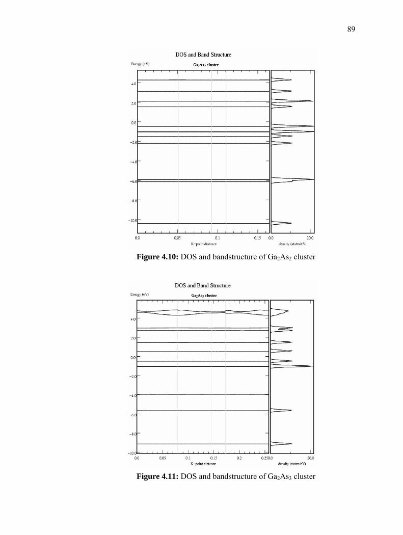
89
Figure 4.10: DOS and bandstructure of Ga2As2 cluster
Figure 4.11: DOS and bandstructure of Ga2As3 cluster

90
Figure 4.12: DOS and bandstructure of Ga3As3 cluster
Figure 4.13: DOS and bandstructure of Ga3As4 cluster

91
Figure 4.14: DOS and bandstructure of Ga4As4 cluster
Figure 4.15: DOS and bandstructure of Ga4As5 cluster

92
Figure 4.16: DOS and bandstructure of Ga5As5 cluster
Figure 4.17: DOS and bandstructure of Ga5As6 cluster

93
Figure 4.18: DOS and bandstructure of Ga6As6 cluster
Figure 4.19: DOS and bandstructure of Ga7As6 cluster
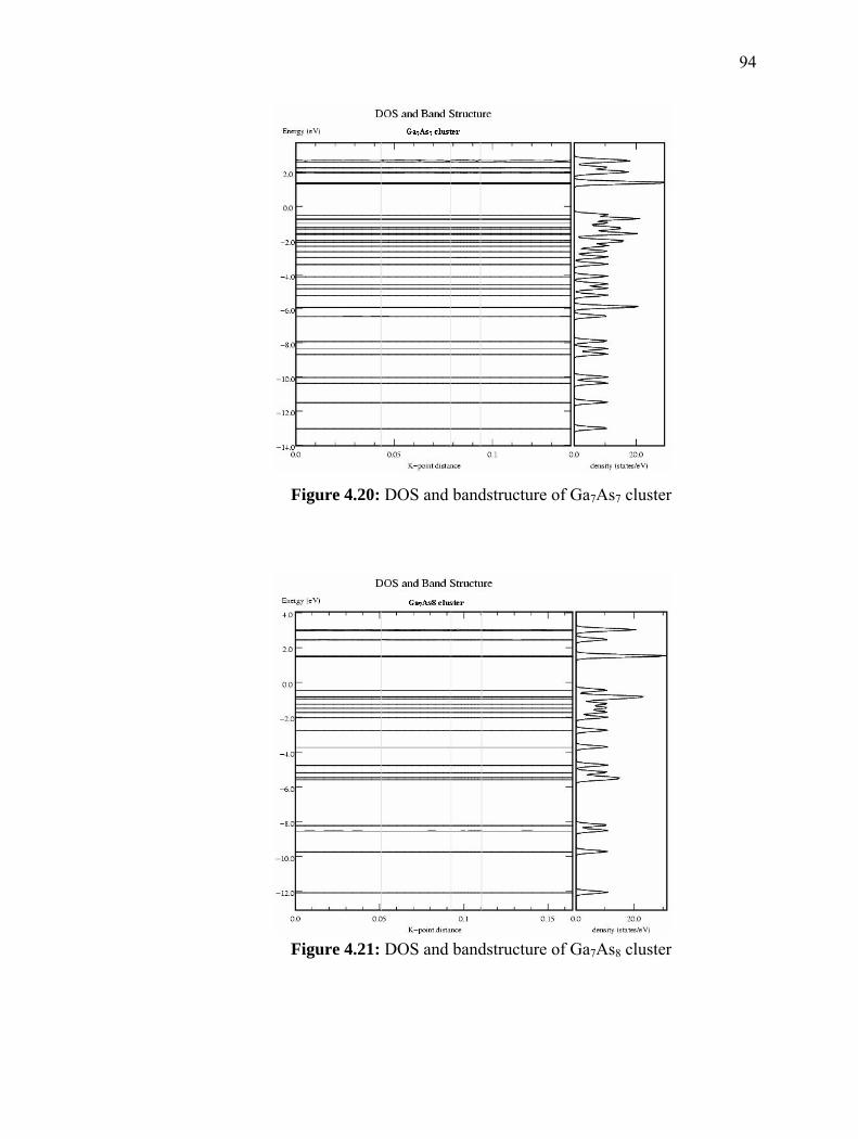
94
Figure 4.20: DOS and bandstructure of Ga7As7 cluster
Figure 4.21: DOS and bandstructure of Ga7As8 cluster

95
Table 4.3: Energy level (HOMO and LUMO) as well as bandgap value of each GaxAsy clusters, (x +y ≤ 15 )
GaxAsy HOMO (eV) LUMO (eV) Bandgap (eV) Ga1As1 -4.329 -3.949 0.38 Ga1As2 -4.473 -4.063 0.41 Ga2As2 -4.356 -3.196 1.16 Ga2As3 -4.783 -3.693 1.09 Ga3As3 -4.325 -2.395 1.93 Ga3As4 -4.294 -3.834 0.46 Ga4As4 -4.392 -3.272 1.12 Ga4As5 -4.211 -3.801 0.41 Ga5As5 -4.584 -2.854 1.73 Ga5As6 -4.205 -3.365 0.84 Ga6As6 -4.117 -3.067 1.05 Ga7As6 -4.287 -3.307 0.98 Ga7As7 -4.311 -3.141 1.17 Ga7As8 -4.195 -3.235 0.96
Bandgap of GaAs Clusters
0
0.5
1
1.5
2
2.5
0 5 10 15 20Number of GaAs Atom
Ene
rgy
Gap
(eV
Our result L.Lou et.al [5]
Figure 4.22: Graph of bandgap versus number of GaAs atom in the cluster and comparison between other researcher’s results [5].

96
Table 4.4: Binding energy per atom of each gallium arsenide cluster, GaxAsy (x + y ≤ 15 ). The binding energies are not corrected with zero potential energies. Reseacher’s data are from reference a[5], b[6] , c[12], d[10], e[80] and f [9].
GaxAsy Binding Energy Per Atom (eV/atom)
Researcher’s Data (eV/atom)
Ga1As1 1.87 1.08a, 2.46b, 2.06±0.05c, 2.206d
Ga1As2 2.14 1.93a, 2.31b, 0.767d
Ga2As2 2.25 2.22a, 2.38b, 0.572d
Ga2As3 2.28 2.40a, 2.87b, 0.387d, 2.95f
Ga3As3 2.31 2.43a, 2.56b, 0.367d, 2.233e, 3.29f
Ga3As4 2.37 2.43a, 2.52b, 0.334d
Ga4As4 2.45 2.54a, 2.55b, 0.673d, 2.379e, 3.35f
Ga4As5 2.48 2.54a, 2.63b
Ga5As5 2.59 2.65a, 2.71b, 2.373e, 3.58f
Ga5As6 2.61 2.393e, 3.59f
Ga6As6 2.69 Ga7As6 2.70 Ga7As7 2.73 2.574e
Ga7As8 2.78
Binding Energy Per Atom of GaAs Clusters
0
0.5
1
1.5
2
2.5
3
0 1 2 3 4 5 6 7 8 9 10 11 12 13 14 15 16
Number of GaAs Atom
Bin
ding
Ene
rgy
Per
Ato
m (e
V/a
tom
Figure 4.23: Graph of binding energy per atom of GaAs clusters.

97
Table 4.5: Second-difference energies and electron affinity of each gallium arsenide cluster, GaxAsy (x + y ≤ 15 ). Researcher’s data are from reference a[5], b[6], c[10] and d[9].
Electron Affinity (eV) GaxAsySecond-difference
Energies (eV) Calculation Researcher’s Data Ga1As1 0.56 1.85 1.9a, 1.9b, 1.24c
Ga1As2 -0.04 2.17 2.1a, 1.9b, 1.31c
Ga2As2 0.28 1.63 1.8a, 1.7b, 1.40c, 1.7d
Ga2As3 -0.11 2.41 2.7a, 2.5b, 1.83c
Ga3As3 0.03 1.72 1.6a, 1.5b, 0.81c, 1.8d
Ga3As4 -1.32 2.69 2.9a, 2.5b, 2.71c
Ga4As4 1.57 2.27 2.8a, 2.4b, 1.46c, 3.3d
Ga4As5 -1.65 3.24 3.5a, 3.1b
Ga5As5 0.96 2.37 2.4a, 2.0b, 2.2d
Ga5As6 -0.46 2.56 Ga6As6 0.51 2.13 2.1d
Ga7As6 -0.27 2.33 Ga7As7 0.22 2.21 Ga7As8 -0.58 2.71
Second-Order Difference Energy and Electron Affinity
-2
-1
0
1
2
3
4
0 5 10 15 20
Number of GaAs Atom
Ene
rgy
(eV
)
2nd-Order DifferenceEnergyElectron Affinity
Figure 4.24: Graph of second-difference energies and electron affinity of each GaxAsy (x + y ≤ 15 ) corresponding to the table above.
98
Figure 4.8 – 4.21 shows the bandstructure and energy spectrum of each of the
gallium arsenide cluster from number of atoms 2 to 15. Obviously similar to the
GaxAsyHz discussed previously, the energy levels of each cluster are discrete
depicting the effect of size and quantum confinement. The corresponding HOMO
and LUMO energy levels as well as the band gap resulted from the HOMO-LUMO
difference is listed in Table 4.3.
The bandgaps of those optimized gallium arsenide clusters do not have a
trend as those for the hydrogenated gallium arsenide clusters, as shown in Figure
4.22. Instead, they have uneven bandgap values and the data point is up and down.
Ga2As2, Ga2As3, Ga3As3, Ga4As4, Ga5As5, Ga6As6 and Ga7As7 a have very large
bandgap values which are above 1.0 eV. Ga1As1 has the lowest bandgap among all
the clusters. Nevertheless, this smallest bandgap is still larger than the bulk gallium
arsenide bandgap (0.354 eV obtained in this research), indicating the effects of
quantum confinement in the small clusters. These bandgap values have a good
agreement with other researchers’ result. As shown in Figure 4.22, the bandgap
values calculated in this research are very close to the results obtained by L. Lou et.al
[5].
Figure 4.23 shows the graph of the binding energies per atom of all clusters.
The energy values shown are not zero-point energy (ZPE) corrected. Binding energy
depicts the energy required to remove an atom from the cluster. Binding energy per
atom is given in terms of the energies of the free gallium arsenide atom and the
cluster:
EB = (nEGa-atom + nEAs-atom) – (Ecluster) (4.1)
99
Where E(Ga), E(As) and E(cluster) are the energies of an isolated Ga atom, a As
atom and the cluster, respectively. An agreement is found between the calculated
and the theoretical binding energy as shown in Table 4.4. The binding energy per
atom rose rapidly from Ga1As1 to Ga1As2 and the slope gradually decreases until it is
nearly horizontal. The size dependence of binding energy is the consequence of the
cluster growth patterns. The very small clusters (x +y ≥ 2-7) tend to have compact
polyhedral geometries, which allow them to maximize their binding energy
effectively [81]. It has been shown that intermediate size clusters (x +y ≥ 8-15) grow
as elongated structures. From Table 4.4 shows that the binding energy per atom
increase as the size of the clusters increases. It is due to the fact that constituent
atoms in larger clusters have more neighbors resulting in strong interactions.
Binding energy graph can be used to study the magic sizes of the clusters.
However, the phenomenon is not obvious and hardly noticeable from the binding
energy graph (Figure 4.23). A better way to show the relative local stability of the
gallium arsenide cluster is through the use of the second-order difference binding
energy (2Δx+y) as a function of cluster size as shown in Figure 4.11. This energy is
obtained by:
2Δx+y
= E(x+y) + 1 + E(x+y) – 1 – 2E(x+y) (4.2)
Notable peaks were observed for GaxAsy clusters with Ga1As1, Ga2As2, Ga3As3,
Ga4As4, Ga5As5, Ga6As6 and Ga7As7 indicating that they are relatively more stable in
comparison with clusters of [(x+y)+1] and [(x+y)-1] atoms. If the highest occupied
electronic subshell is filled in a cluster of (x + y) atoms, and the next available
subshell is separated by a sizable energy gap, the cluster energy will jump from E(x+y)
to E(x+y)+1, which gives rise to peak indicating the cluster of size n is very stable. This
result has proved the validity of the cluster stability obtained from binding energy
graph.

100
Another method to determine the relative stability is through electron affinity.
Electron affinity is a measure of the energy change when an electron is added to a
neutral atom to form a negative ion. Thus it is calculated by:
EA = EN – EN+1 = E(neutral) - E(anion) = E(GaxAsy) – E( ) (4.3) −yAsGax
where N is the number of electrons of the system or cluster. The electron affinity
calculated here is vertical electron affinity which is equal to the energy difference of
the cluster GaxAsy and its anion in the equilibrium geometry of the Ga−yAsGax xAsy.
The result shows smaller electron affinities are yielded for Ga1As1, Ga2As2, Ga3As3,
Ga4As4, Ga5As5, Ga6As6 and Ga7As7. Conversely, Ga1As2, Ga2As3, Ga3As4, Ga4As5,
Ga5As6, Ga7As6 and Ga7As8 have larger electron affinities than their adjacent
clusters.
This result is in opposite trend with the second-order difference energies. The
higher peaks for the second-order difference energies are those lower peaks for the
electron affinities (Ga1As1, Ga2As2, Ga3As3, Ga4As4, Ga5As5, Ga6As6 and Ga7As7).
The gallium arsenide clusters with smaller electron affinities are more stable than
their neighbors. The GaxAsy clusters have shown that the electronic affinity (EA) of
gallium arsenide clusters with the number of atoms (x + y); the even-numbered
clusters tend to have smaller EA and the odd-numbered clusters have larger EA [82].
The vertical electron affinity is in correspondence with the LUMO energy
level. Referring to Table 4.5, it can be observed that the clusters with higher LUMO
energy level have smaller vertical electron affinity and vice versa. Those with higher
LUMO are the highly stable clusters. Ga1As2, Ga2As3, and Ga3As4 and Ga4As5 have
lower LUMO level and therefore its vertical electron affinity is higher. Adiabatic
electron affinity [10] which is the energy difference of GaxAsy and its corresponding

101
anion, had given a much smaller electron affinity value for Ga−yAsGax 1As2 and
Ga2As3. Gallium Arsenide cluster with 5 atoms, Ga2As3 has lower adiabatic electron
affinity than Ga3As4 which has additional bonding in its anion contributing to a fairly
high electron affinity [10]. Most photoelectron spectroscopy corresponds to the
adiabatic electron affinity. Nonetheless, vertical electron affinity yielded in this
research gave a good stability trend for gallium arsenide clusters. The goal here is to
understand the trends in the electron affinities as a function of the size of the clusters.
From the graphs, it can be concluded that the stable clusters obtained are
Ga1As1, Ga2As2, Ga3As3, Ga4As4, Ga5As5, Ga6As6 and Ga7As7. Stability of Ga3As3 is
more obvious in the electron affinity graph than in the second-order difference graph.
These stability studies contribute to the “magic number” of the gallium arsenide
cluster where the highly stable clusters are the magic clusters.
The bandgap of the gallium arsenide clusters can be related with their
stability discussed above. It can be noted that the clusters with large bandgap have
high stability. This is especially obvious for GaxAsy with Ga2As2, Ga3As3, Ga4As4,
Ga5As5, Ga6As6 and Ga7As7, for which these are the magic clusters. However, this is
not the case for Ga1As1 and Ga2As3, where Ga1As1 which is more stable has
comparative lower bandgap and while larger bandgap for Ga2As3 which are less
stable. Therefore, the relation between the stability and bandgap can be applied for
clusters with the number of atom after 5. The interpretation could be made such that
the ground state stability was derived by having significant bonding which splits the
HOMO and LUMO as much as possible. An ambiguous relation can also be made
with the geometries of the gallium arsenide clusters. From Figure 4.7, it could be
observed that GaxAsy with Ga2As3, Ga3As3, Ga3As4, Ga5As5 and Ga6As6 have more
compact, nearly spherical and higher symmetrical geometries. Ga1As2 and Ga2As2
for which their structures are more open and flat have small bandgap.

102
4.4 Effect of Hydrogen and Reconstructed Surface to Electronic Structures
The results of hydrogenated and stable ground state gallium arsenide clusters
could be compared as in Table 4.6. The bandgap values for pristine gallium arsenide
clusters similar to those in Figure 4.3 with hydrogen atoms eliminated and without
optimization, were also included in the table. Only gallium arsenide clusters GaxAsy
with (x +y) = 8, 11 and 13 were taken for comparison.
Bandgap (eV) Number of atom,
x, y, and z GaxAsy (non-
optimized) GaxAsyHz
GaxAsy (surface
reconstructed)
(x = 4), (y = 4), (z = 12) 0.48 7.34 0.92 (x = 5), (y = 6), (z = 16) 0.65 4.42 1.23 (x = 7), (y = 6), (z = 16) 0.31 3.58 0.98
Table 4.6: Bandgap (eV) comparison of bare non-optimized tetrahedral GaAs clusters, hydrogenated GaAs clusters and surface reconstructed GaAs clusters.
(x = 7), (y = 6), ( z = 19) 0.31 1.92 0.98
The bandgap values for 3 types of gallium arsenide cluster show obvious
difference between each other, where hydrogenated gallium clusters have the largest
bandgap followed by optimized gallium clusters and lastly non-optimized gallium
arsenide clusters. For unpassivated and non-optmized gallium clusters having
tetrahedron bonding as bulk gallium , the bandgaps were found to be very small that
they are even smaller than the bandgap of bulk gallium arsenide (0.354 eV). These
clusters tend to be metallic. This phenomenon is due to the surface state of the
unpassivated gallium arsenide clusters that have dangling bonds at the surface. It is a
consequence of the missing neighbors at the surface. Each dangling bond contributes
a partially filled surface state and these states are located in the energy gap around
the Fermi level. This has been well demonstrated for the surface of bulk gallium

103
arsenide using a number of methods including high resolution electron energy loss
spectroscopy [83,84] and photoemission [85], which show that surface states mostly
fill the bandgap of the unpassivated gallium arsenide surface. Therefore, it results in
a much smaller bandgap.
When the clusters with non-relaxed surface atoms and very low average
coordination numbers, as described above is relaxed and optimized, dissimilar
geometries are likely to be produced, in which the tetrahedron bonds symmetry of
bulk gallium arsenide have been broken. The surface atoms (dangling bonds)
contributing surface tension provide a large driving force to form more compact
structures provided the resulting strain energy is not too high.
Therefore the dangling atoms reconstructed by creating bonds with other
atoms and this leads to a stable configurations with large portion of atoms are on the
surface. The dangling bonds and thus the surface states near the Fermi level are
significantly reduced via the reconstruction. New states appear due to the geometry
reconstruction at the outer shell and generally the occupied states shift toward more
negative side while the virtual (unoccupied) states shift towards more positive side.
As a result, the clusters have larger bandgap compared to the pristine cluster with
high density of dangling bonds. However, the reconstruction does not eliminate the
dangling bonds completely. Hence, the reconstructed gallium arsenide surface still
contains a large amount of dangling bonds and shows chemical reactivity which is
somewhat smaller compared to the bulk. This is the reason of the random energy gap
values which is independent of the cluster size.
The results for gallium arsenide clusters passivated with hydrogen are
entirely different from the two types of bare clusters discussed previously. The
passivated gallium arsenide clusters do not show low energy transitions associated

104
with surface states but show much broader bandgaps just as expected for particles in
this extremely small size range. The dangling bonds on the surface which exist in the
bare cluster have now been eliminated or passivated by hydrogen atoms which
complete the four coordination number of gallium arsenide atoms. The surface atoms
do not give any new surface geometry formation and retain their original shape.
Since all the dangling bonds of the surface atoms are passivated, no surface state is
introduced within the energy gap.
The bandgap depends only on the size effect, rather than on the surface effect.
The dependence of electronic structure variations on the size effect has important
consequences especially on the optical properties which are controllable with size.
The bandgap increases as the size decreases, implying that radiation or emission
from quantum dot “blue-shifted” reflecting the fact that electron must fall a greater
distance in terms of energy (from conduction band to valence band) and thus produce
radiation of a shorter wavelength. The size-dependent emission frequency gives rise
to a very important development of optical devices in which the output wavelength
and therefore the output color can be controlled precisely by controlling the size of
the quantum dot. Passivation with oxygen has further consequences for the particles
[86]. Surface passivation and absorption with different passivants are likely to give
different impact on the electronic structures.
The discussions above gave an evidence that the electronic structures of
gallium arsenide clusters could be influenced by plenty of factors. The bandgap is
found to be strongly dependent on the factors as below:
i.) Surface passivation
ii.) Surface reconstruction
iii.) Surface orientation
iv.) Passivation with species other than hydrogen

CHAPTER 5
SUMMARY AND CONCLUSION
5.1 Summary and Conclusion
The electronic structure of gallium arsenide clusters have been presented.
The electronic structures were simulated by using VASP, a simulation package
which is based on the principle of density functional theory (DFT). In this research,
structural properties of gallium arsenide clusters were also studied.
Simulation of bulk gallium arsenide has shown that the density functional
theory underestimates the bandgap value. It has been claimed that the result is due to
the discontinuity in the DFT exchange-correlation functional derivatives. The
simulation shows the bandgap of 0.354 eV for gallium arsenide, which is 1.07 eV
lower than the experimental value, 1.424 eV. However, geometry optimization done
by DFT has produced quite accurate structures. Although DFT has underestimated
the bandgap, it still give excellent qualitative results for insights on nanostructures.
The bandgap underestimation does not demonstrate the failure of DFT since it is a

106
ground state theory and the bandgap is an excited state property. DFT produces good
energy and excellent structure while scaling favorably with electron number and
hence it is feasible on larger systems compared to other methods. Besides, it offers
notable balance between accuracy and computational cost in which it produces
accurate results with relatively smaller basis sets in comparison with other method
such as Hartree-Fock . The success of DFT is also due to its availability of
increasingly accurate approximations to the exchange-correlation energy. It is able to
give the quantitative understanding of materials properties from the fundamental
laws of quantum mechanics.
The simulation of hydrogenated gallium arsenide clusters was done to study
the size effect to electronic structures of the clusters. Bandgap and density of states
(DOS) were studied particularly. The energy quantization is shown by the discrete
spectrum of DOS. It is called discrete energy spectrum instead of density of states
which has continuous density. It shows the evolution of electronic structures of the
clusters in comparison to bulk solids. From the graph of bandgap versus number of
gallium arsenide atom, it is found that the bandgap increases with the decrement of
the cluster sizes in term of the number of gallium arsenide atoms. This dependence of
bandgap to the size of cluster is in agreement with the theory of nanostructures.
The lowest-energy structures of gallium arsenide clusters, GaxAsy (x + y ≤
15) have been studied. The ground state structure of each cluster has entirely
different structure with the tetrahedral bond structure of bulk gallium arsenide.
Unlike hydrogenated gallium arsenide cluster, the bandgap values for these ground
state clusters do not have a particular trend either increasing or decreasing. Instead,
the bandgap values are up and down. Binding energy, second-order difference
energy, and electron affinity were also studied for the ground state gallium arsenide
clusters. These three analyses could show the local relative stability of the gallium
arsenide cluster. The results show that Ga1As1, Ga2As2, Ga3As3, Ga4As4, Ga5As5,

107
Ga6As6 and Ga7As7 are more stable in comparison with their neighbors. When the
stability was related to the bandgap, it was found that the clusters with larger
bandgap (>1.0 eV) have higher stability, such as Ga2As2, Ga3As3, Ga4As4, Ga5As5,
Ga6As6 and Ga7As7. However, it is found that Ga2As3 cluster has lower stability
although it has a bandgap larger than 1.0 eV. The Ga1As1 is more stable and it has
the smallest bandgap with 0.38 eV. Nonetheless, it is still larger than the bulk
bandgap value (0.354 eV).
Comparing the hydrogenated gallium arsenide clusters with the bare ground
state gallium arsenide clusters, it has been observed that the former have much larger
bandgap in comparison with the latter. Another simulation results has showed that
for the unrelaxed gallium arsenide clusters with tetrahedron bonds extracted from
bulk gallium arsenide, their bandgaps are very small that they are even smaller than
the bulk bandgap value and is approximately zero. This smaller bandgap of bare
gallium arsenide clusters compared to the fully passivated gallium arsenide clusters
is due to the dangling bonds. The dangling bonds introduce extra states in the energy
gap near Fermi level which reduces the bandgap.
From the results obtained, it could be concluded that gallium arsenide clusters
in nano-size have novel electronic structures that differ from the bulk gallium
arsenide. The electronic structures of the gallium arsenide clusters can be affected by
the surface reconstruction and also the surface passivations. Therefore, the bandgap
of the clusters can be controlled by manipulating their size and shapes. These
properties of clusters have contributed to the unique attributes of the novel
transistors such as single electron transistor (SET). The objectives of this research
have been achieved and this could be a good foundation for further research, for
instance the study the electron transport in SET.

108
5.2 Suggestions
Some suggestions are given in the following to improve the research. These are the
improvement in bandgap accuracy and computational time.
5.2.1 Improvement of the Bandgap Accuracy
Since DFT underestimates the bandgap value in semiconductor, other
approximation could be taken to improve the accuracy. For example, Green’s
function and the screened Coulomb interaction approximation have been applied as
the correction to DFT bandgaps [88]. Besides this, Quantum Monte Carlo (QMC)
approach for calculating electronic structures would give more accurate results for
the bandgap. QMC is an important and complementary alternative to density
functional theory when performing computational electronic structure calculations in
which high accuracy is required. The method has many attractive features for
probing the electronic structure of real atom, molecules and solids. In particular, it is
a genuine many-body theory with a natural and explicit description of electron
correlation which gives consistent, highly-accurate results while at the same time
exhibiting favorable (cubic or better) scaling of computational cost with system size.
The most important characteristics and advantages of the QMC methodology can be
summarized as follows:

109
(a) it gives a direct and accurate wave-function-based treatment of quantum
many-body effects.
(b) it is a very general approach, applicable to solids and molecules and able to
calculate almost any ground-state expectation value, including energies and
static correlation functions.
(c) the N3 scaling of the computational cost is very favorable when compared
with other correlated wave-function methods. N is the number of particles. In
contrast, Monte Carlo simulations for the ground state of many-body systems
scale as N3 so that they can be applied to sufficiently large systems to allow
extrapolation to the bulk limit.
(d) it has the significant computational advantages of easily achieved scalability
on parallel architectures and low storage requirements.
(e) the diffusion monte carlo (DMC) method does not suffer from the basis set
errors inherent in other correlated wave-function methods.
5.2.2. Improvement of the Computation Time
Ab-initio calculations are accurate but computationally expensive. The
representation of structures by unit cells is the reason leads to redundancies within
the high dimensional search space. To shorten the computation time, more high
power computation units (CPUs) are needed. This problem can be solved by parallel
computing, which is the simultaneous execution of the same task on multiple
processors in order to obtain results faster. A problem can be divided into smaller
task and broken down to a series of instructions. These instructions from each task
execute simultaneously on different CPUs.

110
Computer cluster is a group of tightly coupled computers that work together
closely so that in many respects they can be viewed as though they are a single
computer. The components of a cluster are commonly connected to each other
through fast local area networks. The cluster built can be categorized as high-
performance cluster (HPC). HPC with nodes running Linux as the open system (OS)
and free software to implement the parallelism is often referred to as a Beowulf
cluster.
To test the performance of the parallelization, two factors were studied,
which are speedup and efficiency. Speedup refers to how much a parallel algorithm
is faster than a corresponding sequential algorithm. It is defined by the following
formula:
NSTTS N
NN ≤≤= 1,1
where N is the number of processors, T1 is the execution time of the sequential
algorithm, and Tp is the execution time of the parallel algorithm with p processors
[89]. Ideal speedup is SN = N, which is called linear speedup. Efficiency is a
performance metric estimating how well-utilized the processors are in solving the
problem compared to how much effort is wasted in communication and
synchronization. It is defined as:
10, ≤≤= NN
N ENS
E
Algorithms with linear speedup and algorithms running on a single processor have an
efficiency of 1.

111
Table 5.1: Execution time, speedup and efficiency of VASP using parallel computing [90].
Number of CPU Execution Time (s) Speedup Efficiency 1 308.447 1 1 2 180.798 1.706031 0.853016 3 131.688 2.342256 0.780752 4 109.984 2.804472 0.701118 5 92.549 3.332797 0.666559 6 80.901 3.812648 0.635441 7 73.709 4.184659 0.597808 8 68.259 4.518774 0.564847 9 65.806 4.687217 0.520802
10 61.958 4.978324 0.497832 11 57.473 5.366816 0.487892
Figure 5.1 and 5.2 show a simple performance benchmark of VASP running
at 2 to 11 CPUs. It is obvious that the execution time for the parallel calculation
reduces as the number of CPU increases (refer to Table 5.1).
Figure 5.1: Graph of total time used for completing a parallel calculation versus the number of CPU.
0
50
100
150
200
250
300
350
0 1 2 3 4 5 6 7 8 9 10 11 12
Number of CPU
Tota
l tim
e (s
)

112
Speedup and Efficiency
0
1
2
3
4
5
6
0 1 2 3 4 5 6 7 8 9 10 11 12
Number of CPU
Spee
dup
0
0.2
0.4
0.6
0.8
1
1.2
Effic
ienc
y
SpeedupEfficiency
Figure 5.2: Graph of speedup and efficiency vs number of CPU.
From the graph, it can be observed that the speedup is not linear. For 11
CPUs, the speedup is 5.4 times faster than the sequential algorithm. Both speedup
and efficiency trends show the decreasing of the speedup and efficiency as the
number of CPU increases. This is owing to the communications between the CPUs
are getting more massive when the number of CPU increases.

113
REFERENCES
[1] S.H. Yang, D.A. Drabold, J.B. Adams, A. Sachdev. Stability, structural
transformation and reactivity of Ga13 clusters. Phys. Rev. B. 2000. 61(11):
7277-7290.
[2] H.K. Quek, Y.P. Feng, C.K. Ong. Tight binding molecular dynamics studies
of GamAsn and AlmAsn clusters. Zeitschrift Für Physik D: Atoms, Molecules
and Clusters. 1997. 42(4): 309-317.
[3] Y.P. Feng, C.K. Ong, H.C. Poon, D. Tomanek. Tight binding molecular
dynamics simulation of semiconductor alloy: Cluster, surfaces and defects.
J. Phys. Condens. Matter. 1997. 9(21): 4345.
[4] K.M. Song, A.K. Ray, P.K. Khowash. On the electronic structure of GaAs
clusters. J. Phys. B: Atomic, Molecular and Optical Physics. 1994. 27(8):
1637-1648.
[5] L. Lou, L.Wang, L.P.F. Chibante, R.T. Laaksonen, P. Nordlander, R.E.
Smalley. Electronic structure of small GaAs clusters. J. Chem. Phys. 1991.
94(12): 8015.
[6] L. Lou, P. Nordlander, R.E. Smalley. Electronic structure of small GaAs
clusters II. J. Chem. Phys. 1992. 97(3): 1858.
[7] M.A. Al-Laham, K. Raghavachari. Theoretical study of small gallium
arsenide clusters. J. Chem. Phys. 1991. 187(2): 13-20.
[8] R.M. Graves, G.E. Scuseria. Ab initio theoretical study of small GaAs
clusters. J. Chem. Phys. 1991. 95(9): 6602.

114
[9] J.-Y. Yi. Atomic and electronic structures of small GaAs clusters. Chem.
Phys. Lett. 2000. 325: 269-274.
[10] P. Piquini, A. Fazzio, S. Canuto. Ab initio self-consistent-field studies of the
structures, energetics and bonding of small gallium arsenide clusters.
Zeitschrift Für Physik D: Atoms, Molecules and Clusters. 1995. 33(2): 125-
131.
[11] M.Z. Liao, D.G. Dai, K. Balasubramanian. Electronic states of the Ga3As2
and Ga2As3 clusters. Chem. Phys. Lett. 1995. 239: 124-130.
[12] G.W. Lemire, G.A. Bishea, S.A. Heidecke, M.D. Morse. Spectroscopy and
electronic structure of jet-cooled GaAs. J. Chem. Phys. 1990. 92(121): 121.
[13] R. Schäfer, S. Schlecht, J. Woenckhaus, J.A. Becker. Polarizabilities of
isolated semiconductor clusters. Phys. Rev. Lett. 1996. 76: 471-474.
[14] J.A. Becker. Molecular beam studies on semiconductor clusters:
Polarizabilities and chemical bonding. Angew. Chem. Int. Ed. 1997. 36(14):
1390-1404.
[15] A. P. Alivisatos. Semiconductor clusters, nanocrystals and quantum dots.
Science, New Series. 1996. 271(5251): 933 – 937.
[16] Jing Shi, S. Gider, K. Babcock, D. D. Awschalow. Magnetic clusters in
molecular beams, metals, and semiconductors. Science, New Series. 1996.
271(5251): 937 – 941.
[17] David J. Wales. Structure, dynamics and thermodynamics of clusters: Tales
from topographic potential surfaces. Science, New Series. 1996. 271(5251):
925 – 929.
[18] Keith D. Ball, R. Stephen Berry, Ralph e. Kenz, Feng-Yin Li, Ana Proykova,
David J. Wales. From topographies to dynamics on multidimensional
potential energy surface of atomic clusters. Science, New Series. 1996.
271(5251): 963 – 966.
[19] K. Liu, J. D. Cruzan, R.J. Saykally. Water Clusters. Science, New Series.
1996. 271(5251): 929 – 933.
[20] Gustavo E. Scuseria. Ab Initio calculations of fullerenes. Science, New
Series. 1996. 271(5251): 942 – 945.

115
[21] P. Piquini, S. Canuto, A. Fazzio. Structural and electronic studies of
Ga3As3, Ga4As3 and Ga3As4. Int. J. Quantum Chem. 1994. 52(S28): 571-577.
[22] P. Korambath, S.P. Karna. (Hyper) polarizabilities of GaN, GaP and GaAs
clusters: An initio time dependent Hartree-Fock study. J. Phys. Chem. A.
2000. 104(20): 4801-4804.
[23] M.A Al-Laham, G.W. Trucks, K. Raghavachari. Theoretical study of small
aluminium phosphide and magnesium sulfide clusters. J. Chem. Phys. 1992.
96(2): 1137.
[24] U. Meier, S.D. Peyerimhoff, F. Grein. Ab initio MRD-CI study of
GaAs,−GaAs 2(±), Ga2As2(±) and As4 clusters. Chem. Phys. 1991. 150(3):
331-351.
[25] P.Y. Feng, K. Balasubramanian. Electronic state of Ga2P2. Chem. Phys. Lett.
1996. 258(4): 387-392.
[26] Serdar Öğüt. First Principles Modeling of Nanostructures. Turkish Journal of
Physics. 2003. 27(5): 443-458.
[27] C. Delerue and M. Lannoo. Nanostructures: Theory and Modelling. Berlin:
Springer. 2004.
[28] Takeyce K. Whittingham. Scaling Relations in Density Functional Theory
and Applications of Electronic Structure Methods. PhD Dissertation. The
State University of New Jersey; 2004.
[29] Attila Szabo and Neil S. Ostlund. Modern Quantum Chemistry: Introduction
to Advanced Electronic Structure Theory. Revised Edition. US: McGraw-
Hill. 2003.
[30] Enrico Lipparini. Modern Many-Particle Physics: Atomic Gases, Quantum
Dots and Quantum Fluids. Singapore: World Scientific, 2003.
[31] L. H. Thomas. The calculation of atomic fields. Proc. Cambrigde Philos.
Soc. 1927. 23: 542.
[32] E. Fermi. Application of statistical gas methods to electronic systems. Atti.
Accad. Naz. Lincei, Cl. Sci. Fis. Mat. Nat. Rend. 1927. 6: 602.
[33] P. A. M. Dirac. Quantum Mechanics of Many-Electron Systems. Proc. Royal
Soc.(London) A. 1929. 123(792): 714-733.

116
[34] S. J. Vosko, L. Wilk and M. Nusair. Accurate spin-dependent electron liquid
correlation energies for local spin density calculations: A critical analysis.
Can. J. Phys. 1980. 58: 1200.
[35] J. P. Perdew and A. Zunger. Self-interaction correction to density-functional
approximations for many-electron systems. Phys. Rev. B. 1982. 23(10):5048-
5079.
[36] D. M. Ceperley and B. J. Alder. Ground State of the Electron Gas by a
Stochastic Method. Phys. Rev. Lett. 1980. 45(7): 566.
[37] P. Hohenberg and W. Kohn, Inhomogeneous Electron Gas. Phys. Rev. 1964.
136(3B): B864 - B871.
[38] J. Kohanoff and N.I. Gidopoulos, Density Functional Theory: Basics, New
Trends and Applications. In: Stephen Wilson. Handbook of Molecular Physics
and Quantum Chemistry. Chichester: John Wiley & Sons. Volume 2, Part 5,
Chapter 26, 532–568; 2003.
[39] D. C. Langreth and M. J. Mehl. Easily Implementable Nonlocal Exchange-
Correlation Energy Functional. Phys. Rev. Lett. 1981. 47(6): 446-450.
[40] Langreth, D.C. and Mehl, M.J. Beyond the local-density approximation in
calculations of ground-state electronic properties. Phys. Rev. B. 1983, 28(4):
1809.
[41] Perdew, J.P. and Wang, Y. Accurate and simple density functional for the
electronic exchange energy: Generalized gradient approximation. Phys. Rev.
B. 1986. 33(12): 8800-8802.
[42] J. P. Perdew. Density-functional approximation for the correlation energy of
the inhomogeneous electron gas,Phys. Rev. B. 1986. 33(12): 8822-8824.
[43] A. D. Becke. Density-functional exchange-energy approximation with correct
asymptotic behavior. Phys. Rev. A. 1988. 38(6): 3098-3100.
[44] Chengteh Lee, Weitao Yang, and Robert G. Parr. Development of the Colle-
Salvetti correlation-energy formula into a functional of the electron density.
Phys. Rev. B. 1988. 37(2): 785-789.
[45] J. P. Perdew and Y. Wang. Accurate and simple analytic representation of
the electron-gas correlation energy. Phys. Rev. B, 1992. 45(23): 13244-13249.

117
[46] J. P. Perdew, Unified Theory of Exchange and Correlation Beyond the Local
Density Approximation. In: P. Ziesche and H. Eschrig. Electronic Structure
of Solids '91, Berlin: Akademie Verlag, 11-20; 1991.
[47] J. P. Perdew, K. Burke and M. Ernzerhof. Generalized Gradient
Approximation Made Simple. Phys. Rev. Lett. 1996. 77(18): 3865-3868.
[48] J. P. Perdew, K. Burke and M. Ernzerhof. Generalized Gradient
Approximation Made Simple. Phys. Rev. Lett.1997. 78: 1396 (E).
[49] Yingkai Zhang and Weitao Yang. Comment on “Generalized Gradient
Approximation Made Simple”. Phys. Rev. Lett. 1998. 80(4): 890 – 890.
[50] M. Levy and J. P. Perdew. Hellmann-Feynman, virial, and scaling requisites
for the exact universal density functionals. Shape of the correlation potential
and diamagnetic susceptibility for atoms, Phys. Rev. A. 1985. 32(4):2010-
2021.
[51] E. H. Lieb and S. Oxford. An Improved Lower Bound on the Indirect
Coulomb Energy. Int. J. Quantum Chem. 1981. 19:427.
[52] R. P. Feynman. Forces in Molecules. Phys. Rev. 1939. 56(4): 340 – 343.
[53] J. C. Slater. Atomic Shielding Constants. Phys. Rev. 1930. 36(1): 57 – 64.
[54] W. J. Hehre, R. F. Stewart, and J. A. Pople. Self-Consistent Molecular Orbital
Methods. I. Use of Gaussian Expansions of Slater Type Atomic Orbitals, J.
Chem. Phys. 1969. 51(6): 2657-2664.
[55] W. J. Hehre, W. A. Lathan, R. Ditchfield, M. D. Newton, and J. A. Pople,
Gaussian 70, Quantum Chemistry Program Exchange, Program No. 237,
1970.
[56] M. T. Yin and Marvin L. Cohen. Theory of ab initio pseudopotential
calculations. Phys. Rev. B. 1982. 25(12): 7403 – 7412.
[57] P. E. Blöch. Projector augmented-wave method. Phys. Rev. B. 1994. 50(24):
17953.
[58] A.R. Tackett, N.A.W. Holzwarth and G.E. Matthews. A Projector
AugmentedWave (PAW) code for electronic structure calculations, Part II:
pwpaw for periodic solids in a plane wave basis. Computer Physics
Communications. 2001. 135(3): 348–376.
118
[59] Georg Kresse and Jürgen Furthmüller. VASP the GUIDE. Institut für
Materialphysik, Universität Wien. 2005. (retrieved from:
http://cms.mpi.univie.ac.at/VASP/)
[60] G. Kresse and J. Joubert. From ultrasoft pseudopotentials to the projector
augmented wave method. Phys. Rev. B. 1999. 59(3): 1758-1775.
[61] H. J. Monkhorst and J. D. Pack. Special points for Brillouin-zone
integrations. Phys. Rev. B. 1976. 13(12): 5188-5192.
[62] R. O. Jones. Cluster Geometries From Density Functional Calculations –
Prospects and Limitations. Eur. Phys. J. D. 1999. 9: 81-84.
[63] N. Metropolis, A.W. Rosenbluth, M.N. Rosenbluth. A.H. Teller and E.
Teller. Equation of State Calculations by Fast Computing Machines. J. Chem.
Phys. 1953. 21(6): 1087-1092.
[64] R.C. Weast. Handbook of Chemistry and Physics. 62nd ed. CRC Press, Inc,
Boca Raton. 1981.
[65] Andréîa Luίsa da Rosa. Density Functional Theory Calculations on Anti-
Surfactants at Gallium Nitride Surface. Master Dissertation. Universität
Berlin; 2003.
[66] G. S. Rohrer. Structure and Bonding in Crystalline Materials. Cambridge
University Press, Cambridge, England. 2001.
[67] Thang B. Hoang, L. V. Titova, H. E. Jackson and L. M. Smith; Imaging and
optical properties of single core-shell GaAs-AlGaAs nanowires. University of
Cineinnati, OH. 2006.
[68] K. Balasubramaniam. Electronic states of GaAs and . J. Chem. Phys.
1987. 86(6): 3410.
+GaAs
[69] G.E. Scuseria. Application of open-shell coupled cluster theory to the ground
state of GaAs. Theor. Chim. Acta. 1991. 80: 215-219.
[70] P. Karamanis, D. Begue and C. Pouchan. Ab initio finite field (hyper)
polarizability computations on stoichiometric gallium arsenide clusters
GanAsn (n = 2-9). J. Chem. Phys. 2007. 127: 094706.
[71] K. Balasubramaniam. Spectroscopic constant for , GaAs−2GaAs 2,
and Ga
−AsGa2
2As. J. Phys. Chem. A. 2000. 104(10): 1969-1973.
119
[72] T. R. Taylor, H. Gomez, K. R. Asmis and D. Neumark. Photoelectron
spectroscopy of , , and (X = P, As). J. Chem.
Phys. 2001. 115: 4620.
−2GaX −XGa2
−22 XGa −
32 XGa
[73] J. J. Belbruno. Bonding and energetics in small clusters of gallium and
arsenic. Heteratomic chem. 2003. 14: 189-196.
[74] S. Brownridge and F. Grein. Geometries, electronic g-tensor elements,
hyperfine coupling constants and vertical excitation energies for small
gallium arsenide doublet radicals, GaxAsy (x + y = 3, 5). J. Phys. Chem. A.
2003. 107(39): 7969-7980.
[75] A. Costales, A. K. Kandalam, R. Franco and R. Pandey. Theoretical study of
structural and vibrational properties of (AlP)n, (AlAs)n, (GaP)n, (GaAs)n,
(InP)n and (InAs)n clusters with n = 1,2,3. J. Phys. Chem. B. 2002. 106: 1940-
1944.
[76] X. Zhu, Spectroscopic properties of gallium arsenide tetramers: Ga2As2,
and . Spectrochim. Acta A. 2005. 61: 2730-2736. +22 AsGa −
22 AsGa
[77] S. Burrill and F. Grein. Structure and bonding of III/V compounds X2Y2 with
X2B, Al, Ga and Y = N, P, As. J. Mol. Struct. Theochem. 2005. 757: 137-
142.
[78] S. Li, R. J. Van Zee and W. Weltner Jr. Hyperfine interaction and structure of
a gallium arsenide cluster: Ga2As3. J. Chem. Phys. 1993. 98: 4335
[79] Bei Liu, Zhong- Yi Liu, Bicai Pan, Cai-Zhuang Wang and Kai-Ming Ho.
Ionization of medium sized clusters and the geometries of the cations. J.
Chem. Phys. 1998. 109(21): 9401 – 9409.
[80] Q. L. Lu, J. C. Jiang, J. G. Wan and G. H. Wang. Density-functional study of
ring-like GanAsn (3≤n≤14) clusters. J. of Molecular Structure. 2008. 851:
271-276.
[81] Thomas Bachels, Rolf Schäfer. Binding energies of neutral silicon clusters.
Chem. Phys. Lett. 2004. 324: 365-372.
[82] C. Jin, K. J. Taylor, J. Conceicao and R. E. Smalley. Ultraviolet
photoelectron spectra of gallium arsenide clusters. Chem. Phys. Lett. 1990.
175: 17-22.
120
[83] D. J. Frankel, C. Yu, J. P. Harbison and H. H. Farell. High- resolution
electron energy loss spectroscopy studies of GaAs (100) surfaces. J. Vac. Sci.
Technol. B .1987. 5(4): 1113-1118.
[84] J. A. Schaefer, T. Allinger, C. Stuhlman, U. Beckers and H. Ibach.
Interaction of hydrogen at GaAs (100) surfaces. Surf. Sci. 1991. 251/252:
1000-1005.
[85] E.D. Lu, Y. Yang, X. J. Zhou, S.A. Kellar, P. V. Bogdanor, A.C. Huan, F.
Cerina, Z. Hussain and Z. X. Shen. Photoemission spectromicroscopy study
on passivation of GaAs (100) by CH3CSNH2 / NH4OH. University Stanford,
Stanford. CA94305.
[86] Ronald Schailey and Asok K. Ray. A cluster approach to hydrogen
chemisorption on the GaAs (100) surface. J. Computational Material
Science. 2001. 22: 169-179.
[87] Asok K. Ray and Michael L. Mayo. An ab initio cluster study of atomic
oxygen chemisorption on Ga-rich GaAs (100) (2x1) and β(4x2) surface:
University of Texas at Arlington, Arlington, Texas 76019.
[88] Kurt A. Johnson and N. W. Ashcraft. Corrections to Density-Functional
Theory Band Gaps. Phys. Rev. B. 1998. 58(23): 15548-15556.
[89] Norahanim Mohd Jais. Ujian Prestasi Pembangunan Makmal Pemprosesan
Selari Dengan Antaramuka Laluan Pesanan (MPI) Kaedah Pengenduran
Berturut-turut Merah Hitam (SOR RED BLACK). Degree Dissertation,
Universiti Teknologi Malaysia; 2002.
[90] Lee Jia Yen. Electronic Structures of Silicon Quantum Dots as Nanoclusters
for Single Electron Transistors. Master Dissertation, Universiti Teknologi
Malaysia; 2008.
[91] P. Pulay. Convergence Acceleration in Iterative Sequences: The Case of SCF
Iteration. Chem. Phys. Lett. 73, 393 (1980) .
[92] P. Pulay and S. Saebo: Variational CEPA: Comparison with Different Many-
body Methods. Chem. Phys. Lett. 117, 37 (1985).

121
APPENDIX A
Parallelization of VASP
Traditionally, software has been written for serial computation executed on a
single computer having a single Central Processing Unit (CPU). A problem is broken
into a discrete series of instructions and carried out one after another. In this case,
only one instruction may execute at any moment in time. Therefore, when a CPU is
given a massive and complex ab-initio calculation, it will take a very long time to
handle and the calculation might fail due to the insufficient memory problem. This
serial computing problem can be solved by parallel computing, which is the
simultaneous execution of the same task on multiple processors in order to obtain
results faster. A problem can be divided into smaller task and broken down to a
series of instructions. These instructions from each task execute simultaneously on
different CPUs.
Parallel version of VASP is available and computer cluster approach (see
Figure 2) is used in this research. Computer cluster is a group of tightly coupled
computers that work together closely so that in many respects they can be viewed as
though they are a single computer. The components of a cluster are commonly
connected to each other through fast local area networks. The cluster built can be
categorized as high-performance cluster (HPC). HPC with nodes running Linux as
the OS and free software to implement the parallelism is often referred to as a
Beowulf cluster.
Figure 1 shows the parallel computing cluster used for VASP calculation in
this research. The following lists the important components including hardware and
software of the Beowulf cluster used for the VASP calculation:
i) 11 units of CPU with Intel 3.06Ghz Pentium 4 Hyper-Threading
ii) Gigabit Ethernet card

122
iii) Gigabit network switch
iv) Operating system of Fedora Core 4
v) MPICH2 for the MPI implementation
Network is an important element in determining the performance of the
parallel cluster. It had been shown that Gigabit cards can reduce the latency (delay-
time for a packet of data to get from one designated point to another) to 30 μs in
comparison to the typical 100 MBit Ethernet based network which shows around 90
μs latency. In consideration of bandwidth (maximum transfer rate limits the
communication speed), VASP uses all-to-all communication.
J O B
Master/Server
Local Area Network
J O B
t1
tN
t2Instruction
t1
tN
t2t1
tN
t2
Client/Slave
Figure 1. Schematic of parallel computing cluster illustrating a master-server distributes a job to 3 client nodes and communication between them is showed.

123
The MPI version of VASP is compiled and installed by using the Fortran 90
of Intel Fortran Compiler (IFC). Therefore, MPICH2 is also compiled by using IFC
before the installation of VASP. Below are the brief descriptions on how to build the
11-nodes Beowulf cluster:
1) The network of the cluster is configured. Hostnames and unique IP addresses
are assigned for each node in the cluster. All the nodes should be in the same
local network. One node is designated as the master node and is assigned IP
address of 192.168.10.101. IP address is added one for each client node
(192.168.10.102, etc.) for easy recognition and there would be no problem as
long as the IP address is in the range of 192.168.10.255. The nodes are named
setpar01 through setpar11 to keep things simple, using setpar01 as the master
node. An identical user account is created in all nodes so that VASP is run as
common user but not root.
2) The communication protocol of the cluster is configured. There are commonly
two protocols which are RSH and SSH. Because of the cluster is exposed to the
public networks, SSH (Secure Shell) is chosen to provide a more secure system
since it encrypts all communication by means of private plus public key
encryption methods. The MPICH2 must be also using SSH protocol.
3) Password-less login is enabled. The communication between the cluster nodes
must be free from password request to ensure a non-barrier environment for
data sending and receiving. This can be done by first enabling the global
cluster node authentication. A database of all nodes' public keys is kept in the
file named ‘ssh_known_hosts’ in the SSH directory and this file is saved in
each of the node. In the second step, the list of all hostnames of the cluster
nodes is created in the file ‘shosts.equiv’ in SSH directory and also list of all
hosts and user who allowed to log in is created in file ‘.shosts’ in home
directory. This is a authentication method combines shosts or shosts.equiv with
RSA-based host authentication. It means that is the login would be permitted
by ~/.shosts or /etc/ssh/shosts.equiv, and additionally it can verify the client’s
host key from /etc/ssh/ssh_known_host, only then login is permitted. This
authentication method closes security holes due to IP spoofing, DNS spoofing
and routing spoofing.

124
4) NFS (Network File System) server and clients is configured. NFS allows hosts
to mount partitions on a remote system and use them as though they are local
file systems. This allows the system administrator to store resources in a
central location on the network, providing authorized users continuous access
to them. Master node is configured to be NFS server and shares the directory of
VASP and MPICH2 with other client nodes.
5) MPICH2 is configured and a file mpd.hosts containing a list of hostnames is
created. The process manager of MPICH2 which is called MPD will start the
MPI jobs on the nodes specified in the file.
6) VASP is run by giving the command ‘mpiexec –np 11 <directory of VASP>’
in the working directory where the calculation is to be run.
Figure 2. Cluster of parallel-computing set up for VASP calculation.

125
Performance of Parallelization
To test the performance of the parallelization of VASP, two factors were
studied, which are speedup and efficiency. Speedup refers to how much a parallel
algorithm is faster than a corresponding sequential algorithm. It is defined by the
following formula:
NSTTS N
NN ≤≤= 1,1
where N is the number of processors, T1 is the execution time of the sequential
algorithm, and Tp is the execution time of the parallel algorithm with p processors
[103]. Ideal speedup is SN = N, which is called linear speedup. Efficiency is a
performance metric estimating how well-utilized the processors are in solving the
problem compared to how much effort is wasted in communication and
synchronization. It is defined as:
10, ≤≤= NN
N ENS
E
Algorithms with linear speedup and algorithms running on a single processor have an
efficiency of 1.
Table 1. Execution time, speedup and efficiency of VASP using parallel computing
Number of CPU Execution Time (s) Speedup Efficiency 1 308.447 1 1 2 180.798 1.706031 0.853016 3 131.688 2.342256 0.780752 4 109.984 2.804472 0.701118 5 92.549 3.332797 0.666559 6 80.901 3.812648 0.635441 7 73.709 4.184659 0.597808 8 68.259 4.518774 0.564847 9 65.806 4.687217 0.520802
10 61.958 4.978324 0.497832 11 57.473 5.366816 0.487892

126
Figure 2 and 3 show a simple performance benchmark of VASP running at 2
to 11 CPUs. It is obvious that the execution time for the parallel calculation reduces
as the number of CPU increases (refer to Table 1).
0
50
100
150
200
250
300
350
0 1 2 3 4 5 6 7 8 9 10 11 12
Number of CPU
Tota
l tim
e (s
)
Figure 2. Graph of total time used for completing a parallel calculation versus the number of CPU.
Speedup and Efficiency
0
1
2
3
4
5
6
0 1 2 3 4 5 6 7 8 9 10 11 12
Number of CPU
Spee
dup
0
0.2
0.4
0.6
0.8
1
1.2
Effic
ienc
y
SpeedupEfficiency
Figure 3. Graph of speedup and efficiency vs number of CPU.
From the graph, it can be observed that the speedup is not linear. For 11
CPUs, the speedup is 5.4 times faster than the sequential algorithm. Both speedup
and efficiency trends show the decreasing of the speedup and efficiency as the
number of CPU increases. This is owing to the communications between the CPUs
are getting more massive when the number of CPU increases.