Volker Britz, P. Jean-Jacques Herings, Arkadi Predtetchinski On the Convergence to the Nash Bargaining Solution for Endogenous Bargaining Protocols RM/12/030

On the Convergence to the Nash Bargaining Solution

for Endogenous Bargaining Protocols

Volker Britz1 P. Jean-Jacques Herings2 Arkadi Predtetchinski3

June 14, 2012

1V. Britz (volker.britz@uclouvain.be), CORE, Universite Catholique de Louvain. This author

would like to thank the Netherlands Organization for Scientific Research (NWO) for financial

support.2P.J.J. Herings (p.herings@maastrichtuniversity.nl), Department of Economics, Maastricht

University. This author would like to thank the Netherlands Organization for Scientific Research

(NWO) for financial support.3A. Predtetchinski (a.predtetchinski@maastrichtuniversity.nl), Department of Economics,

Maastricht University. This author would like to thank the Netherlands Organization for Scien-

tific Research (NWO) for financial support.

Abstract

We consider non-cooperative multilateral bargaining games with endogenous bargaining

protocols. Under an endogenous protocol, the probability with which a player becomes the

proposer in a round of bargaining depends on the identity of the player who previously

rejected. An important example is the frequently studied rejector-becomes-proposer pro-

tocol. We focus on subgame perfect equilibria in stationary strategies which are shown to

exist and to be efficient. Equilibrium proposals do not depend on the probability to propose

conditional on the rejection by another player, though equilibrium acceptance sets do de-

pend on these probabilities. Next we consider the limit, as the bargaining friction vanishes.

In case no player has a positive probability to propose conditional on his rejection, each

player receives his utopia payoff conditional on being recognized and equilibrium payoffs

are in general Pareto inefficient. Otherwise, equilibrium proposals of all players converge to

a weighted Nash Bargaining Solution, where the weights are determined by the probability

to propose conditional on a rejection.

Keywords: Strategic Bargaining, Subgame Perfect Equilibrium, Stationary Strate-

gies, Nash Bargaining Solution

JEL codes: C78

1 Introduction

This paper examines the convergence of equilibrium payoffs in a non-cooperative bargaining

game to the asymmetric Nash bargaining solution. In contrast to the existing literature

on this topic, we allow for the proposer selection to be endogenous, that is, influenced by

the players’ actions throughout the game.

We contribute to the so-called Nash program, a research agenda which investigates

the relationship between solution concepts from the cooperative (axiomatic) and non-

cooperative (strategic) branches of game theory. The classic example is the treatment

of the bargaining problem by Nash (1950, 1953). The bargaining problem here refers to a

situation where two players can choose one element of a convex set of feasible payoff pairs

by mutual consent. If they fail to agree, an exogenously given pair of disagreement payoffs

will realize. The Nash bargaining solution is that payoff pair which maximizes the product

of players’ gains over their disagreement payoff. Nash (1950) shows that this is the unique

bargaining solution satisfying the axioms of scale invariance, symmetry, efficiency, and

independence of irrelevant alternatives. Nash (1953) presents a non-cooperative demand

game with two players who are uncertain about which payoff pairs are feasible. In the

limit as uncertainty vanishes, equilibrium payoffs converge to those predicted by the Nash

bargaining solution. In another seminal paper, Rubinstein (1982) also obtains convergence

of equilibrium payoffs to the Nash Bargaining Solution, but in a bargaining game with

alternating offers. In their discussion of cooperative and non-cooperative approaches to

bargaining, Binmore, Rubinstein, and Wolinsky (1986) obtain the Nash bargaining solu-

tion in the limit if either players’ impatience or the risk of an exogenous breakdown of the

negotiations is vanishing.

The asymmetric Nash bargaining solution (Kalai 1977) maximizes a weighted product

of players’ gains over the disagreement payoffs. It reduces to the Nash bargaining solution

when the weights are equal across players. Moreover, it is straightforward to generalize

the asymmetric Nash bargaining solution to the case with an arbitrary number of players.

However, the analysis of non-cooperative bargaining games with more than two players

presents substantial difficulties as long as one insists on unanimity.1 In multilateral una-

nimity bargaining, one typically obtains a wide multiplicity of subgame-perfect equilibrium

payoffs. Much of the literature has dealt with this multiplicity by restricting attention to

subgame-perfect equilibria in stationary strategies. This restriction allows for a unique

1There is a branch of literature which circumvents the complications involved in bargaining with more

than two players by relaxing the unanimity rule, particularly by allowing partial agreements. Examples

of such an approach can be found in Krishna and Serrano (1996), Chae and Yang (1994), and Suh and

Wen (2006). In the paper at hand, however, we are interested in situations where a comprehensive and

unanimous agreement is required.

1

prediction of the limit of equilibrium payoff allocations. In this vein, Hart and Mas-Colell

(1996) give an early support result for the Nash bargaining solution. Kultti and Vartiainen

(2010) consider the extension of the model of Rubinstein (1982) to an arbitrary number

of players and assume that proposers rotate according to some fixed order. They show

convergence to the Nash bargaining solution in the limit. Extensions of the Rubinstein

model where the proposer is selected in each period according to a time-invariant proba-

bility distribution, support the asymmetric Nash bargaining solution with the probability

distribution as the weight vector as has been demonstrated by Laruelle and Valenciano

(2008) and Miyakawa (2008). All these results are special cases of Britz, Herings, and

Predtetchinski (2010), who model the proposer selection process as a Markov chain, and

obtain convergence to the asymmetric Nash bargaining solution where the weight vector is

given by the stationary distribution of the Markov chain. All these proposer selection pro-

tocols are exogenous in the sense that the actions of the players in the game have no effect

on the identity of the next proposer. To the best of our knowledge, the entire literature

that has provided non-cooperative support for the asymmetric Nash bargaining solution

considers exogenous protocols only.

Restricting attention to exogenous protocols, however, seems to be a serious limitation.

More in particular, the proposer selection may be influenced by the identity of the player

who rejects a particular proposal. One simple and intuitively appealing example is the

protocol where the player who rejects the current proposal is automatically called to make

the next proposal. This rejector-becomes-proposer protocol has been introduced in Selten

(1981) and has been studied extensively in both the bargaining and the coalition formation

literature, see for example Chatterjee, Dutta, Ray, and Sengupta (1993), Bloch (1996), Ray

and Vohra (1999), Imai and Salonen (2000), and Bloch and Diamantoudi (2011) to name

a few. Of course, this protocol reduces to Rubinstein’s alternating offers model when there

are only two players.

The protocol we study in this paper is more general than the rejector-becomes-proposer

protocol. Following Kawamori (2008), we are interested in the case where the identity of the

player who rejects a proposal may influence the probability by which a particular player

becomes the next proposer. Clearly, the rejector-becomes-proposer protocol is a special

case of the protocol we consider. Another special case is the protocol where a rejector

proposes in the next period with probability zero. It is the polar opposite of the rejector-

becomes-proposer protocol, and can be intuitively justified by the idea that one may want

to design a protocol which discourages rejections by punishing them with a zero recognition

probability. Moreover, also the protocol with time-invariant recognition probabilities is a

special case of the analysis in this paper. In general, however, our protocol does depend

on the approval/rejection decisions of the players involved in the bargaining process, and

2

is therefore indeed endogenous.

Endogenous protocols are considerably more difficult to analyze than exogenous ones,

and the literature has identified a number of cases where both types of protocol lead to

surprisingly different results. For instance, Chatterjee, Dutta, Ray, and Sengupta (1993)

provide examples for non-existence of equilibria as well as existence of equilibria with

delay in the context of an endogenous protocol. On the contrary, it has been shown in

Okada (1996) that delay cannot occur at equilibrium and in Okada (2011) that equilibria

exist when the protocol is exogenous. Similarly, there are examples for non-existence

of equilibrium in Bloch (1996) under an endogenous protocol while Herings and Houba

(2010) restore existence for an exogenous proposer selection protocol. Duggan (2011)

present a very general coalitional bargaining model where equilibrium existence is shown for

exogenous protocols. The paper points out that a similar approach to establish equilibrium

existence would not work when the protocol is endogenous.

Our main findings are as follows. We first consider the payoff allocations that are sup-

ported by subgame-perfect equilibria in stationary strategies. We show that for any value

of the continuation probability such an equilibrium exists, that equilibria are characterized

by the absence of delay, and that all equilibrium proposals specify a Pareto efficient payoff

allocation, results that would not carry over to the more general environment of coali-

tional bargaining as evidenced by the examples in Chatterjee, Dutta, Ray, and Sengupta

(1993). Equilibrium proposals do not depend on the probability to propose conditional on

the rejection by another player, though equilibrium acceptance sets do depend on these

probabilities.

Regarding results on the limit of equilibrium payoffs as the continuation probability

tends to one, we find a distinction between two cases. If none of the players has a positive

probability of being the next proposer after his own rejection, then the proposer in the

initial round obtains his utopia payoff, that is his highest payoff in the set of feasible

payoffs that satisfy all the individual rationality constraints. Since the initial proposer

is selected according to some given probability distribution, the utilities are in general

not Pareto efficient, and do therefore not correspond to an asymmetric Nash bargaining

solution. Otherwise, we find convergence of the equilibrium payoffs to a weighted Nash

bargaining solution, where the weights are determined by the probabilities of making a

counter-offer. Players with a zero probability of making a counter-offer will receive a

payoff of zero.

The existence of equilibria in stationary strategies and the convergence to a weighted

Nash bargaining solution are established results under exogenous protocols and we show

that they carry over to our setting with an endogenous protocol if and only if there is at

least one player with a strictly positive recognition probability conditional on his rejection.

3

However, we see that the bargaining weights depend only on part of the data on the

recognition probabilities. In particular, for the limit bargaining equilibrium payoffs it is

only relevant with what probability a player proposes after his own rejection. Conversely,

it is not important with what probability a player proposes after another player’s rejection.

Moreover, we find that the payoff allocation in the limit bargaining equilibrium exhibits a

discontinuity when the probabilities of making a counter-offer are zero for all players. In

that case, the initial proposer has all the bargaining power, and hence the expected payoffs

depend on the probability distribution which determines the proposer of the first round.

Romer and Rosenthal (1978) is among the most influential papers emphasizing the role

of proposal making on the selected alternative. Kalandrakis (2006) shows in a bargain-

ing framework that the proposer selection process is more important than voting rights,

impatience, or complex equilibrium strategies in explaining political power. Empirical sup-

port for this feature in the context of the allocation of transportation funds in the US is

provided by Knight (2005). The existing results on non-cooperative bargaining games are

for exogenous protocols only and do not distinguish between the probability of making a

proposal and the probability of making a proposal conditional on a rejection. Our paper

argues that the latter probabilities are the ones that really matter to explain bargaining

power.

The paper is organized as follows. Section 2 presents the bargaining game with an

endogenous protocol. Section 3 presents a characterization of the set of subgame perfect

equilibria in stationary strategies. Section 4 introduces the concept of a bargaining equilib-

rium, a selection of the subgame perfect equilibria in stationary strategies. It is shown that,

in payoff terms, the set of bargaining equilibria is equivalent to the set of subgame perfect

equilibrium in stationary strategies. It is also shown that a bargaining equilibrium exists.

Section 5 studies the case where conditional on his rejection, there is zero probability that a

player becomes a proposer, and shows an inefficiency result for this case. Section 6 studies

the limit bargaining equilibrium for the complementary case and presents the convergence

to the asymmetric Nash bargaining solution. Section 7 presents an example to illustrate

the discontinuity in the limit bargaining equilibrium payoffs. Section 8 concludes.

2 The Bargaining Game

We consider a bargaining game between finitely many players. The set of players is

N = {1, . . . , n}. Each player individually can only attain a disagreement payoff which

we normalize to zero. However, the players can jointly achieve any payoff vector v in a set

V ⊂ Rn if they unanimously agree on such a payoff vector. Each player is assumed to be

an expected utility maximizer. The set V of feasible payoffs and the bargaining protocol

4

are the main primitives of the model. We now introduce each in turn.

For vectors u and v in Rn, we write u ≥ v if ui ≥ vi for all i ∈ N, u > v if u ≥ v and

u = v, and u ≫ v if ui > vi for all i ∈ N. A point v of V is said to be Pareto–efficient if

there is no point u in V such that u > v. A point v of V is said to be weakly Pareto–efficient

if there is no point u in V such that u ≫ v. We write V+ to denote the set V ∩ Rn+.

Our first assumption is as follows:

[A1] The set V is closed, convex, and comprehensive from below. There is a point v ∈ V

such that v ≫ 0. The set V+ is bounded. Each weakly Pareto–efficient point of V+ is

Pareto–efficient.

We will denote by P the set of Pareto-efficient points of V and write P+ for the set

P ∩ Rn+.

Bargaining takes place in discrete time t = 0, 1, . . .. There are n+ 1 probability distri-

butions on the players denoted by π0, π1, . . . , πn, each of which belongs to the unit simplex

∆n in Rn.

In round t = 0, a particular player is chosen as the proposer according to the probability

distribution π0 ∈ ∆n. The proposer then makes a proposal v ∈ V . Player 1 responds to the

proposal by either acceptance or rejection. Once a player i = 1, . . . , n− 1 has accepted the

proposal, it is the turn of player i+ 1 to accept or to reject.2 Once player n has accepted

the proposal, the game ends and the approved proposal is implemented.

As soon as some player j ∈ N rejects a proposal in round t, the game ends with prob-

ability 1− δ > 0 and payoffs to all players are zero. With the complementary probability

δ, the game continues to round t + 1. The proposer in that round is then drawn from

the probability distribution πj. If the game continues perpetually without agreement, the

payoff to every player is zero.

In case π0, π1, . . . , πn all coincide, we are back in the familiar case of an exogenous proto-

col with time-invariant recognition probabilities. The rejector-becomes-proposer protocol

follows from specifying πii = 1 for all i ∈ N. A polar opposite of the rejector-becomes-

proposer protocol, where a rejector proposes with probability zero in the next round,

follows by setting πii = 0 for all i ∈ N.

It is well-known that bargaining games with more than two players admit a wide multi-

plicity of subgame perfect equilibria (SPE), see Herrero (1985) and Haller (1986). We will

therefore restrict attention to SPE in stationary strategies (SSPE). A stationary strategy

for player i consists of a proposal θi ∈ V which i makes whenever it is his turn to propose

2Throughout the paper, for the sake of simplicity, we assume that players respond to a proposal in the

fixed order 1, . . . , n. We show in the appendix that all results carry over to the case with arbitrary voting

orders.

5

and an acceptance set Ai ⊂ V which consists of all the proposals which player i would

be willing to accept if they were offered to him. We denote the social acceptance set by

A = ∩i∈NAi and write the profile of stationary strategies (θ1, A1, . . . , θn, An) more concisely

as (Θ,A).

3 Subgame Perfect Equilibria in Stationary Strategies

In this section, we consider the set of SSPEs of the bargaining game. Fix some profile of

stationary strategies (Θ,A). By definition of a stationary strategy, there is a unique payoff

vector which is expected in any subgame following a rejection by some player i ∈ N. We

refer to it as the vector of continuation payoffs after i’s rejection and denote it by qi(Θ,A).

Since it will be clear from the context, we omit the argument in the sequel. Moreover,

we define a vector r(Θ,A) of reservation payoffs by r(Θ,A) = (q11, . . . , qnn). Again, we will

omit the argument in the sequel. It is important to note at this stage that the endogenous

protocol which we consider induces a disparity between the continuation and the reservation

payoffs. Depending on the identity of the player who rejects the current proposal, one out

of n different continuation payoff vectors will realize. When these n vectors are thought

of as the columns of a matrix, the reservation payoffs correspond to its diagonal. If the

protocol is exogenous, all the columns of this matrix are identical since the sequel of the

game is then not influenced by the identity of the rejector. We will see that the reservation

payoffs are important as an “acceptance threshold” in a sense to be made precise in the

next two lemmas.

For every i ∈ N , let S(i) = {j ∈ N |j ≥ i}. That is, S(i) is the set of players succeedingplayer i in the response order, including i himself. We denote ∩j∈S(i)A

j by AS(i).

Lemma 3.1 Let (Θ,A) be an SSPE inducing reservation payoffs r. It holds that

1. If v ∈ V is such that vn > rn, then v ∈ An.

2. For every i = 1, . . . , n− 1, if v ∈ AS(i+1) and vi > ri, then v ∈ Ai.

Proof: Consider a history of the game where player n has to respond to the proposal

v with vn > rn. If player n accepts, the proposal passes and he receives vn. If he rejects,

he expects to receive rn, so he would have a profitable deviation at this history. This

establishes the first part of the lemma. Now consider a history of the game where player

i ∈ N\{n} has to respond to the proposal v with vi > ri and i ∈ AS(i+1). If player i accepts

v, this proposal passes and he receives vi. Otherwise, he receives ri, so he would have a

profitable deviation at this history. �

6

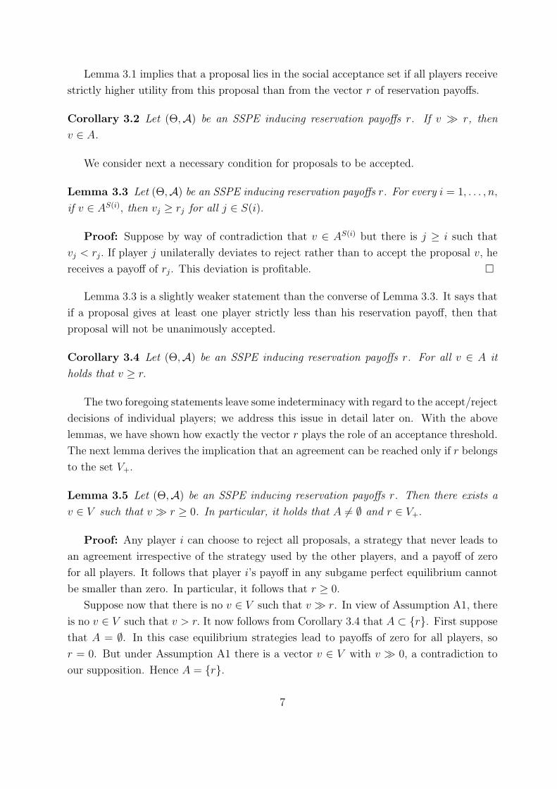
Lemma 3.1 implies that a proposal lies in the social acceptance set if all players receive

strictly higher utility from this proposal than from the vector r of reservation payoffs.

Corollary 3.2 Let (Θ,A) be an SSPE inducing reservation payoffs r. If v ≫ r, then

v ∈ A.

We consider next a necessary condition for proposals to be accepted.

Lemma 3.3 Let (Θ,A) be an SSPE inducing reservation payoffs r. For every i = 1, . . . , n,

if v ∈ AS(i), then vj ≥ rj for all j ∈ S(i).

Proof: Suppose by way of contradiction that v ∈ AS(i) but there is j ≥ i such that

vj < rj. If player j unilaterally deviates to reject rather than to accept the proposal v, he

receives a payoff of rj. This deviation is profitable. �

Lemma 3.3 is a slightly weaker statement than the converse of Lemma 3.3. It says that

if a proposal gives at least one player strictly less than his reservation payoff, then that

proposal will not be unanimously accepted.

Corollary 3.4 Let (Θ,A) be an SSPE inducing reservation payoffs r. For all v ∈ A it

holds that v ≥ r.

The two foregoing statements leave some indeterminacy with regard to the accept/reject

decisions of individual players; we address this issue in detail later on. With the above

lemmas, we have shown how exactly the vector r plays the role of an acceptance threshold.

The next lemma derives the implication that an agreement can be reached only if r belongs

to the set V+.

Lemma 3.5 Let (Θ,A) be an SSPE inducing reservation payoffs r. Then there exists a

v ∈ V such that v ≫ r ≥ 0. In particular, it holds that A = ∅ and r ∈ V+.

Proof: Any player i can choose to reject all proposals, a strategy that never leads to

an agreement irrespective of the strategy used by the other players, and a payoff of zero

for all players. It follows that player i’s payoff in any subgame perfect equilibrium cannot

be smaller than zero. In particular, it follows that r ≥ 0.

Suppose now that there is no v ∈ V such that v ≫ r. In view of Assumption A1, there

is no v ∈ V such that v > r. It now follows from Corollary 3.4 that A ⊂ {r}. First supposethat A = ∅. In this case equilibrium strategies lead to payoffs of zero for all players, so

r = 0. But under Assumption A1 there is a vector v ∈ V with v ≫ 0, a contradiction to

our supposition. Hence A = {r}.

7

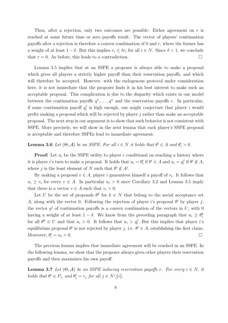
Then, after a rejection, only two outcomes are possible: Either agreement on r is

reached at some future time or zero payoffs result. The vector of players’ continuation

payoffs after a rejection is therefore a convex combination of 0 and r, where the former has

a weight of at least 1− δ. But this implies ri ≤ δri for all i ∈ N . Since δ < 1, we conclude

that r = 0. As before, this leads to a contradiction. �

Lemma 3.5 implies that at an SSPE a proposer is always able to make a proposal

which gives all players a strictly higher payoff than their reservation payoffs, and which

will therefore be accepted. However, with the endogenous protocol under consideration

here, it is not immediate that the proposer finds it in his best interest to make such an

acceptable proposal. This complication is due to the disparity which exists in our model

between the continuation payoffs q1, . . . , qn and the reservation payoffs r. In particular,

if some continuation payoff qji is high enough, one might conjecture that player i would

prefer making a proposal which will be rejected by player j rather than make an acceptable

proposal. The next step in our argument is to show that such behavior is not consistent with

SSPE. More precisely, we will show in the next lemma that each player’s SSPE proposal

is acceptable and therefore SSPEs lead to immediate agreement.

Lemma 3.6 Let (Θ,A) be an SSPE. For all i ∈ N it holds that θi ∈ A and θii > 0.

Proof: Let ui be the SSPE utility to player i conditional on reaching a history where

it is player i’s turn to make a proposal. It holds that ui = θii if θi ∈ A and ui = qji if θ

i /∈ A,

where j is the least element of N such that θi /∈ Aj.

By making a proposal v ∈ A, player i guarantees himself a payoff of vi. It follows that

ui ≥ vi for every v ∈ A. In particular ui > 0 since Corollary 3.2 and Lemma 3.5 imply

that there is a vector v ∈ A such that vi > 0.

Let U be the set of proposals θk for k ∈ N that belong to the social acceptance set

A, along with the vector 0. Following the rejection of player i’s proposal θi by player j,

the vector qj of continuation payoffs is a convex combination of the vectors in U , with 0

having a weight of at least 1 − δ. We know from the preceding paragraph that ui ≥ θkifor all θk ∈ U and that ui > 0. It follows that ui > qji . But this implies that player i’s

equilibrium proposal θi is not rejected by player j, i.e. θi ∈ A, establishing the first claim.

Moreover, θii = ui > 0. �

The previous lemma implies that immediate agreement will be reached in an SSPE. In

the following lemma, we show that the proposer always gives other players their reservation

payoffs and then maximizes his own payoff.

Lemma 3.7 Let (Θ,A) be an SSPE inducing reservation payoffs r. For every i ∈ N, it

holds that θi ∈ P+ and θij = rj for all j ∈ N\{i}.

8

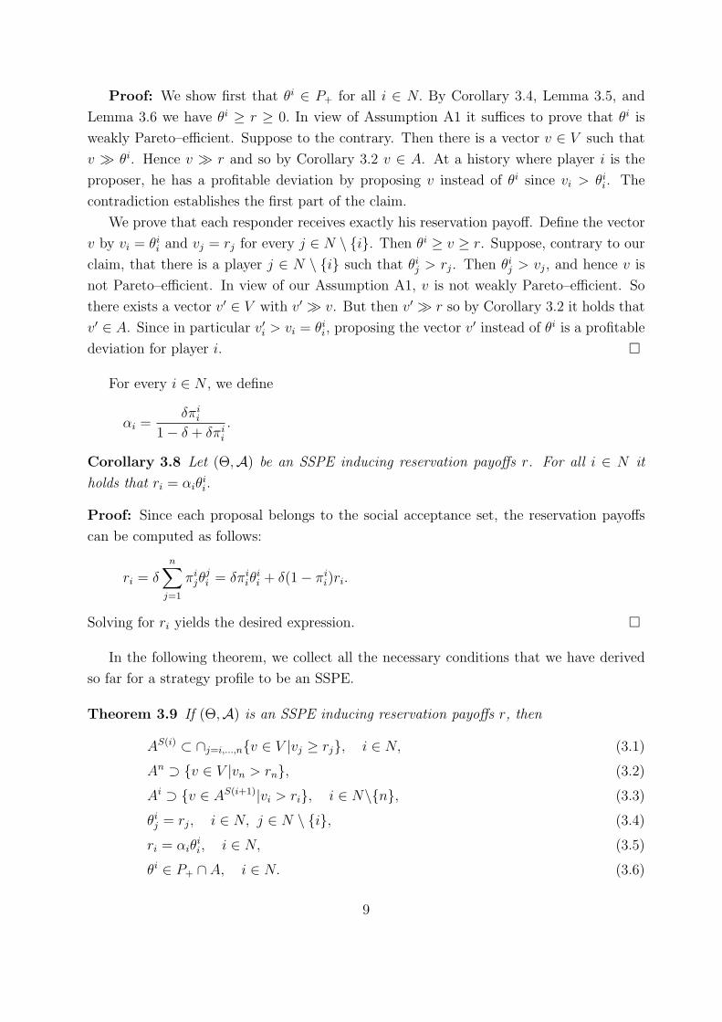
Proof: We show first that θi ∈ P+ for all i ∈ N. By Corollary 3.4, Lemma 3.5, and

Lemma 3.6 we have θi ≥ r ≥ 0. In view of Assumption A1 it suffices to prove that θi is

weakly Pareto–efficient. Suppose to the contrary. Then there is a vector v ∈ V such that

v ≫ θi. Hence v ≫ r and so by Corollary 3.2 v ∈ A. At a history where player i is the

proposer, he has a profitable deviation by proposing v instead of θi since vi > θii. The

contradiction establishes the first part of the claim.

We prove that each responder receives exactly his reservation payoff. Define the vector

v by vi = θii and vj = rj for every j ∈ N \ {i}. Then θi ≥ v ≥ r. Suppose, contrary to our

claim, that there is a player j ∈ N \ {i} such that θij > rj. Then θij > vj, and hence v is

not Pareto–efficient. In view of our Assumption A1, v is not weakly Pareto–efficient. So

there exists a vector v′ ∈ V with v′ ≫ v. But then v′ ≫ r so by Corollary 3.2 it holds that

v′ ∈ A. Since in particular v′i > vi = θii, proposing the vector v′ instead of θi is a profitable

deviation for player i. �

For every i ∈ N , we define

αi =δπi

i

1− δ + δπii

.

Corollary 3.8 Let (Θ,A) be an SSPE inducing reservation payoffs r. For all i ∈ N it

holds that ri = αiθii.

Proof: Since each proposal belongs to the social acceptance set, the reservation payoffs

can be computed as follows:

ri = δn∑

j=1

πijθ

ji = δπi

iθii + δ(1− πi

i)ri.

Solving for ri yields the desired expression. �

In the following theorem, we collect all the necessary conditions that we have derived

so far for a strategy profile to be an SSPE.

Theorem 3.9 If (Θ,A) is an SSPE inducing reservation payoffs r, then

AS(i) ⊂ ∩j=i,...,n{v ∈ V |vj ≥ rj}, i ∈ N, (3.1)

An ⊃ {v ∈ V |vn > rn}, (3.2)

Ai ⊃ {v ∈ AS(i+1)|vi > ri}, i ∈ N\{n}, (3.3)

θij = rj, i ∈ N, j ∈ N \ {i}, (3.4)

ri = αiθii, i ∈ N, (3.5)

θi ∈ P+ ∩ A, i ∈ N. (3.6)

9

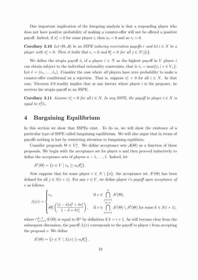
One important implication of the foregoing analysis is that a responding player who

does not have positive probability of making a counter-offer will not be offered a positive

payoff. Indeed, if πii = 0 for some player i, then αi = 0 and so ri = 0.

Corollary 3.10 Let (Θ,A) be an SSPE inducing reservation payoffs r and let i ∈ N be a

player with πii = 0. Then it holds that ri = 0 and θij = 0 for all j ∈ N\{i}.

We define the utopia payoff vi of a player i ∈ N as the highest payoff in V player i

can obtain subject to the individual rationality constraints, that is vi = max{vi | v ∈ V+}.Let v = (v1, . . . , vn). Consider the case where all players have zero probability to make a

counter-offer conditional on a rejection. That is, suppose πii = 0 for all i ∈ N . In that

case, Theorem 3.9 readily implies that at any history where player i is the proposer, he

receives his utopia payoff in an SSPE.

Corollary 3.11 Assume πii = 0 for all i ∈ N. In any SSPE, the payoff to player i ∈ N is

equal to π0i vi.

4 Bargaining Equilibrium

In this section we show that SSPEs exist. To do so, we will show the existence of a

particular type of SSPE called bargaining equilibrium. We will also argue that in terms of

payoffs nothing is lost by restricting attention to bargaining equilibria.

Consider proposals Θ ∈ V n+ . We define acceptance sets A(Θ) as a function of these

proposals. We begin with the acceptance set for player n and then proceed inductively to

define the acceptance sets of players n− 1, . . . , 1. Indeed, let

An(Θ) = {v ∈ V | vn ≥ αnθnn} .

Now suppose that for some player i ∈ N \ {n}, the acceptance set Aj(Θ) has been

defined for all j ∈ S(i + 1). For any v ∈ V , we define player i’s payoff upon acceptance of

v as follows:

βi(v) =

vi, if v ∈

n∩j=i+1

Aj(Θ),

δθii

((1− δ)πk

i + δπii

1− δ + δπii

), if v ∈

k−1∩j=i+1

Aj(Θ) \ Ak(Θ) for some k ∈ S(i+ 1),

where ∩k−1j=i+1A

j(Θ) is equal to Rn by definition if k = i+ 1. As will become clear from the

subsequent discussion, the payoff βi(v) corresponds to the payoff to player i from accepting

the proposal v. We define

Ai(Θ) ={v ∈ V | βi(v) ≥ αiθ

ii

}.

10

The construction of acceptance sets A(Θ) is now complete. We denote by A(Θ) the con-

comitant social acceptance set, that is, the intersection of the sets Ai(Θ), i = 1, . . . , n.

Definition 4.1 A bargaining equilibrium is a strategy profile (Θ,A(Θ)) such that for all

i ∈ N,

θi ∈ P+, (4.1)

θij = αjθjj , j ∈ N \ {i}. (4.2)

Since the coefficients αi do not depend on πij for j = i, we see that the equilibrium pro-

posals in a bargaining equilibrium do not depend on the probability to propose conditional

on the rejection by another player. As is clear from the construction above, equilibrium

acceptance sets do depend on these probabilities.

We show next that in a bargaining equilibrium there is no delay before reaching an

agreement.

Theorem 4.2 In a bargaining equilibrium (Θ,A(Θ)), agreement is reached immediately:

for all i ∈ N, θi ∈ A(Θ).

Proof: We prove the result by induction. For i ∈ N \ {n}, we have θin = αnθnn, so

θi ∈ An(Θ). For i = n, since αn < 1, we have θnn ≥ αnθnn, so θn ∈ An(Θ).

Now suppose that for some player j ∈ N \ {n} it holds that θi ∈ Ak(Θ) for all k ∈S(j + 1). We show that θi ∈ Aj(Θ) thereby completing the proof.

By the induction hypothesis it holds that βj(θi) = θij. For i ∈ N \ {j}, we have

βj(θi) = θij = αjθ

jj ,

so θi ∈ Aj(Θ). For i = j, since αj < 1, we have

βj(θj) = θjj ≥ αjθ

jj ,

so θj ∈ Aj(Θ). �

Since bargaining equilibrium proposals do not depend on the probability to propose

conditional on the rejection by another player, and equilibrium proposals are accepted

without delay, it follows that the equilibrium utility depends on the initial recognition

probabilities π0 and on the probability to propose conditional on an own rejection πii, but

not on the probabilities πij for j = i.

Another important feature of a bargaining equilibrium is that there is an advantage to

being the proposer. To see this, simply notice that αi < 1, so that θij < θii for j = i.

11

The continuation payoff to player i after a rejection of a proposal by player k can be

computed as follows:

qki (Θ,A(Θ)) = δ

n∑j=1

πkj θ

ji = δπk

i θii + δ(1− πk

i )

(δπi

i

1− δ + δπii

)θii

= δθii

((1− δ)πk

i + δπii

1− δ + δπii

).

The reservation payoffs are given by

ri(Θ,A(Θ)) = qii(Θ,A(Θ)) = αiθii.

In a bargaining equilibrium, each responder receives precisely his reservation payoff. The

payoff βi(v) upon acceptance of v is vi if v ∈ Aj(Θ) for every player j ∈ S(i+ 1) and it is

qki otherwise, where k is the lowest indexed player in S(i+ 1) with v /∈ Ak(Θ). Thus βi(v)

is the payoff to i from accepting the proposal v. Player i accepts the proposal v if and only

if βi(v) ≥ ri.

For v to be an element of the social acceptance set A(Θ) in a bargaining equilibrium,

it should hold that vi ≥ αiθii for all i ∈ N. Indeed, when v ∈ A(Θ), we have that βi(v) = vi

for all i ∈ N, so v ∈ Ai(Θ) implies vi ≥ αiθii for all i ∈ N. It is also easily verified that the

converse is true, if vi ≥ αiθii for all i ∈ N, then v ∈ A(Θ). It follows that in a bargaining

equilibrium (Θ,A(Θ)),

A(Θ) = {v ∈ V | ∀i ∈ N, vi ≥ αiθii}.

We now discuss the relationship between SSPE and bargaining equilibrium. We show

that each bargaining equilibrium is an SSPE. While an SSPE need not be a bargaining

equilibrium, it induces one in a natural way. Intuitively, a bargaining equilibrium can be

thought of as an SSPE that breaks the indifference in the accept/reject decisions in favor of

acceptance. Our results imply that in as much as we are interested in equilibrium proposals

and payoffs rather than acceptance sets, there is no loss in focussing the analysis on the

set of bargaining equilibria rather than the set of SSPEs.

Theorem 4.3 A bargaining equilibrium is an SSPE.

Proof: Let (Θ,A(Θ)) be a bargaining equilibrium. By definition, the bargaining equi-

librium is a profile of stationary strategies. We show that it is a subgame perfect equilib-

rium. Applying the one-shot deviation property, we have to show that at any history the

acting player has no profitable one-shot deviation.

Consider first a one-shot deviation in the accept/reject decisions. By construction of

A(Θ), a responder accepts a proposal if and only if accepting makes him weakly better off

than rejecting. Hence, a one-shot deviation cannot be profitable.

12

Now consider a one-shot deviation by player i, who proposes some v ∈ V \{θi}. Supposethat v ∈ A(Θ). Then, the expected payoff to player i from proposing v is qki where k is

the first player in the response order to reject v. It follows from the expression for the

continuation payoffs given above that

qki = δθii

((1− δ)πk

i + δπii

1− δ + δπii

)≤ δθii ≤ θii,

so the deviation is not profitable. Now consider the case where v ∈ A(Θ). Then vj ≥ αjθjj

for every j ∈ N and hence vj ≥ θij for every j ∈ N \ {i}. Since the vector θi is Pareto–

efficient, we must have vi ≤ θii. Again, the deviation is not profitable. �

Theorem 4.4 If (Θ,A) is an SSPE, then (Θ,A(Θ)) is a bargaining equilibrium.

Proof: Condition (4.1) of Definition 4.1 is implied by Condition (3.6) of Theorem 3.9.

Condition (4.2) is implied by Conditions (3.4)–(3.6) of Theorem 3.9. �

By Condition (3.6) of Theorem 3.9 it holds that there is immediate agreement in any

SSPE. It therefore follows from Theorems 4.3 and 4.4 that the distinction between SSPE

and bargaining equilibrium is immaterial. The set of SSPE utilities coincides with the set

of bargaining equilibrium utilities. It follows in particular that SSPE utilities depend on

the initial recognition probabilities π0 and on the probability to propose conditional on an

own rejection πii, but not on the probabilities πi

j for j = i.

Theorem 4.5 A bargaining equilibrium exists.

Proof: Let us define ρ ∈ ∆n and λ ∈ [0, 1) as follows. If πii > 0 for at least one i ∈ N ,

then

ρi =πii∑n

j=1 πjj

, i ∈ N,

λ =δ∑n

i=1 πii

1−δ+δ∑n

i=1 πii.

If πii = 0 for all i ∈ N , then we set λ = 0 and ρi = 1

nfor all i ∈ N . After elemen-

tary calculus, it follows from Definition 4.1 that the system of characteristic equations

describing bargaining equilibrium proposals of our model with recognition probabilities

π0, π1, . . . , πn and continuation probability δ coincides with the system of characteristic

equations which describes equilibrium proposals in a bargaining model with time-invariant

recognition probabilities ρ and continuation probability λ. The existence of a solution to

the latter system has been shown by Banks and Duggan (2000) in their Theorems 1 and

2.3 �3In Banks and Duggan (2000) the continuation probability is 1, and players have time preferences with

a discount factor equal to δ. Voting is simultaneous rather than sequential, and attention is restricted

to stage-undominated voting strategies. For the case with time-invariant recognition probabilities, both

modeling choices lead to exactly the same equilibrium conditions on proposals as in Definition 4.1.

13

We have shown that a bargaining equilibrium is an SSPE, so the existence of an SSPE

is implied by the theorem above.

Corollary 4.6 An SSPE exists.

5 No Possibility to Propose after a Rejection

In this section we study the case where conditional on a rejection there is zero probability

to be selected as a proposer, so πii = 0 for every player i ∈ N. Corollary 3.11 states that

in any SSPE the payoff to player i ∈ N is equal to π0i vi. Notice that this expression is

independent of the continuation probability δ. Moreover, in case P+ is not a simplex, i.e.

P+ cannot be written as the convex hull of n extreme points, and each player has a positive

probability to be the initial proposer, equilibrium payoffs are in the interior of the set V

and therefore inefficient.

Theorem 5.1 Assume P+ is not a simplex, πii = 0 for all i ∈ N, and π0 ≫ 0. All SSPEs

are inefficient.

Proof: By Corollary 3.11 it holds that SSPE utilities are equal to∑

i∈N π0i vie(i),

where e(i) denotes the i-th unit vector in Rn. Since P+ is not a simplex, there is p ∈P+ \ conv({vie(i) | i ∈ N}), where conv(X) denotes the convex hull of a set of points X.

Choose weights λi ∈ R, i ∈ N, such that p =∑

i∈N λivie(i). Since p ≥ 0, it holds that

λi ≥ 0 for all i ∈ N. It then follows that∑

i∈N λi > 1, since∑

i∈N λi < 1 contradicts the

Pareto optimality of p, and∑

i∈N λi = 1 implies p ∈ conv({vie(i) | i ∈ N}), leading to a

contradiction as well.

Take γ > 0 sufficiently small such that π0 − γλ ≥ 0. Notice that non-negativity of

π0 − γλ implies that γ < 1. We define µ ∈ ∆ by

µ =1

1− γ(π0 − γλ) +

γ(∑

i∈N λi − 1)

1− γe(1),

and v ∈ conv({vie(i) | i ∈ N}) ⊂ V by

v =∑i∈N

µivie(i).

By convexity of V it holds that γp+ (1− γ)v ∈ V. Straightforward calculus shows that

γp+ (1− γ)v = (π01 + γ(

∑i∈N

λi − 1))v1e(1) +∑

i∈N\{1}

π0i vie(i).

Since∑

i∈N λi − 1 > 0 and γ > 0 it holds that γp+ (1− γ)v is a point in V which Pareto

dominates the vector of SSPE utilities. �

14

Although at first glance it might appear as a good idea to deny players the right to

make a proposal following a rejection, Theorem 5.1 claims that the contrary is the case.

Since such protocols give all bargaining power to the initial proposer, the equilibrium result

is a lottery where player i receives his utopia payoff vi with probability π0i and a payoff

of 0 with probability 1 − π0i , leading to inefficient equilibrium utilities when players are

risk-averse, or, more generally, when P+ is not a simplex.

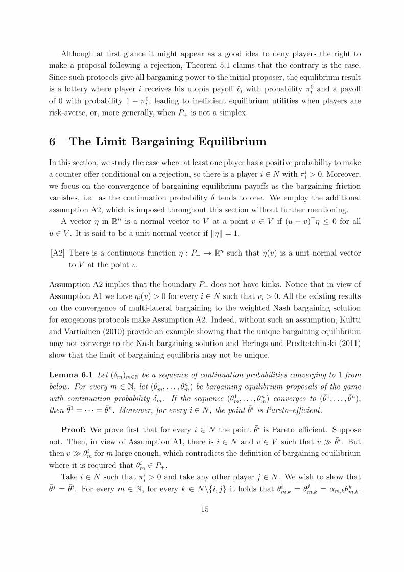
6 The Limit Bargaining Equilibrium

In this section, we study the case where at least one player has a positive probability to make

a counter-offer conditional on a rejection, so there is a player i ∈ N with πii > 0. Moreover,

we focus on the convergence of bargaining equilibrium payoffs as the bargaining friction

vanishes, i.e. as the continuation probability δ tends to one. We employ the additional

assumption A2, which is imposed throughout this section without further mentioning.

A vector η in Rn is a normal vector to V at a point v ∈ V if (u − v)⊤η ≤ 0 for all

u ∈ V . It is said to be a unit normal vector if ∥η∥ = 1.

[A2] There is a continuous function η : P+ → Rn such that η(v) is a unit normal vector

to V at the point v.

Assumption A2 implies that the boundary P+ does not have kinks. Notice that in view of

Assumption A1 we have ηi(v) > 0 for every i ∈ N such that vi > 0. All the existing results

on the convergence of multi-lateral bargaining to the weighted Nash bargaining solution

for exogenous protocols make Assumption A2. Indeed, without such an assumption, Kultti

and Vartiainen (2010) provide an example showing that the unique bargaining equilibrium

may not converge to the Nash bargaining solution and Herings and Predtetchinski (2011)

show that the limit of bargaining equilibria may not be unique.

Lemma 6.1 Let (δm)m∈N be a sequence of continuation probabilities converging to 1 from

below. For every m ∈ N, let (θ1m, . . . , θnm) be bargaining equilibrium proposals of the game

with continuation probability δm. If the sequence (θ1m, . . . , θnm) converges to (θ1, . . . , θn),

then θ1 = · · · = θn. Moreover, for every i ∈ N , the point θi is Pareto–efficient.

Proof: We prove first that for every i ∈ N the point θi is Pareto–efficient. Suppose

not. Then, in view of Assumption A1, there is i ∈ N and v ∈ V such that v ≫ θi. But

then v ≫ θim for m large enough, which contradicts the definition of bargaining equilibrium

where it is required that θim ∈ P+.

Take i ∈ N such that πii > 0 and take any other player j ∈ N . We wish to show that

θj = θi. For every m ∈ N, for every k ∈ N\{i, j} it holds that θim,k = θjm,k = αm,kθkm,k.

15

Taking the limit as m goes to infinity yields θik = θjk. Furthermore, for every m ∈ N, wehave θjm,i = αm,iθ

im,i. Since αm,i converges to one as m tends to infinity, we obtain θji = θii.

We conclude that the vectors θi and θj can only differ in component j. Since both points

θi and θj are Pareto–efficient, we have θi = θj, as desired. �

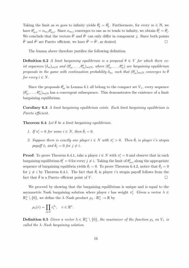
The lemma above therefore justifies the following definition.

Definition 6.2 A limit bargaining equilibrium is a proposal θ ∈ V for which there ex-

ist sequences (δm)m∈N and (θ1m, . . . , θnm)m∈N, where (θ1m, . . . , θ

nm) are bargaining equilibrium

proposals in the game with continuation probability δm, such that (θim)m∈N converges to θ

for every i ∈ N .

Since the proposals θim in Lemma 6.1 all belong to the compact set V+, every sequence

(θ1m, . . . , θnm)m∈N has a convergent subsequence. This demonstrates the existence of a limit

bargaining equilibrium.

Corollary 6.3 A limit bargaining equilibrium exists. Each limit bargaining equilibrium is

Pareto efficient.

Theorem 6.4 Let θ be a limit bargaining equilibrium.

1. If πii = 0 for some i ∈ N, then θi = 0.

2. Suppose there is exactly one player i ∈ N with πii > 0. Then θi is player i’s utopia

payoff vi and θj = 0 for j = i.

Proof: To prove Theorem 6.4.1, take a player i ∈ N with πii = 0 and observe that in each

bargaining equilibrium θji = 0 for every j = i. Taking the limit of θjm,i along the appropriate

sequence of bargaining equilibria yields θi = 0. To prove Theorem 6.4.2, notice that θj = 0

for j = i by Theorem 6.4.1. The fact that θi is player i’s utopia payoff follows from the

fact that θ is a Pareto–efficient point of V . �

We proceed by showing that the bargaining equilibrium is unique and is equal to the

asymmetric Nash bargaining solution where player i has weight πii. Given a vector λ ∈

Rn+ \ {0}, we define the λ–Nash product ρλ : Rn

+ → R by

ρλ(v) =∏i∈N

vλii , v ∈ Rn.

Definition 6.5 Given a vector λ ∈ Rn+ \ {0}, the maximizer of the function ρλ on V+ is

called the λ–Nash bargaining solution.

16

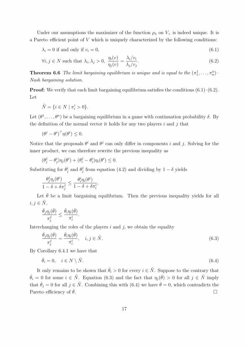
Under our assumptions the maximizer of the function ρλ on V+ is indeed unique. It is

a Pareto–efficient point of V which is uniquely characterized by the following conditions:

λi = 0 if and only if vi = 0, (6.1)

∀i, j ∈ N such that λi, λj > 0,ηi(v)

ηj(v)=

λi/viλj/vj

. (6.2)

Theorem 6.6 The limit bargaining equilibrium is unique and is equal to the (π11, . . . , π

nn)–

Nash bargaining solution.

Proof: We verify that each limit bargaining equilibrium satisfies the conditions (6.1)–(6.2).

Let

N = {i ∈ N | πii > 0}.

Let (θ1, . . . , θn) be a bargaining equilibrium in a game with continuation probability δ. By

the definition of the normal vector it holds for any two players i and j that

(θj − θi)⊤η(θi) ≤ 0.

Notice that the proposals θi and θj can only differ in components i and j. Solving for the

inner product, we can therefore rewrite the previous inequality as

(θjj − θij)ηj(θi) + (θji − θii)ηi(θ

i) ≤ 0.

Substituting for θij and θjj from equation (4.2) and dividing by 1− δ yields

θjjηj(θi)

1− δ + δπjj

≤ θiiηi(θi)

1− δ + δπii

.

Let θ be a limit bargaining equilibrium. Then the previous inequality yields for all

i, j ∈ N ,

θjηj(θ)

πjj

≤ θiηi(θ)

πii

.

Interchanging the roles of the players i and j, we obtain the equality

θjηj(θ)

πjj

=θiηi(θ)

πii

, i, j ∈ N . (6.3)

By Corollary 6.4.1 we have that

θi = 0, i ∈ N \ N . (6.4)

It only remains to be shown that θi > 0 for every i ∈ N . Suppose to the contrary that

θi = 0 for some i ∈ N . Equation (6.3) and the fact that ηj(θ) > 0 for all j ∈ N imply

that θj = 0 for all j ∈ N . Combining this with (6.4) we have θ = 0, which contradicts the

Pareto–efficiency of θ. �

17

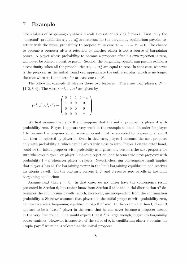
7 Example

The analysis of bargaining equilibria reveals two rather striking features. First, only the

“diagonal” probabilities π11, . . . , π

nn are relevant for the bargaining equilibrium payoffs, to-

gether with the initial probability to propose π0 in case π11 = · · · = πn

n = 0. The chance

to become a proposer after a rejection by another player is not a source of bargaining

power. A player whose probability to become a proposer after his own rejection is zero,

will never be offered a positive payoff. Second, the bargaining equilibrium payoffs exhibit a

discontinuity when all the probabilities π11, . . . , π

nn are equal to zero. In that case, whoever

is the proposer in the initial round can appropriate the entire surplus, which is no longer

the case when πii is non-zero for at least one i ∈ N.

The following example illustrates these two features. There are four players, N =

{1, 2, 3, 4}. The vectors π1, . . . , π4 are given by

(π1, π2, π3, π4

)=

0 1 1 1− ε

1 0 0 0

0 0 0 0

0 0 0 ε

.

We first assume that ε > 0 and suppose that the initial proposer is player 4 with

probability zero. Player 4 appears very weak in the example at hand. In order for player

4 to become the proposer at all, some proposal must be accepted by players 1, 2, and 3

and then be rejected by player 4. Even in that case, player 4 becomes the next proposer

only with probability ε, which can be arbitrarily close to zero. Player 1 on the other hand,

could be the initial proposer with probability as high as one, becomes the next proposer for

sure whenever player 2 or player 3 makes a rejection, and becomes the next proposer with

probability 1 − ε whenever player 4 rejects. Nevertheless, our convergence result implies

that player 4 has all the bargaining power in the limit bargaining equilibrium and receives

his utopia payoff. On the contrary, players 1, 2, and 3 receive zero payoffs in the limit

bargaining equilibrium.

Assume next that ε = 0. In that case, we no longer have the convergence result

presented in Section 6, but rather know from Section 5 that the initial distribution π0 de-

termines the equilibrium payoffs, which, moreover, are independent from the continuation

probability δ. Since we assumed that player 4 is the initial proposer with probability zero,

he now receives a bargaining equilibrium payoff of zero. In the example at hand, player 3

appears to be a “weak” player in the sense that he can never become a proposer except

in the very first round. One would expect that if δ is large enough, player 3’s bargaining

power vanishes. However, irrespective of the value of δ, in equilibrium player 3 obtains his

utopia payoff when he is selected as the initial proposer.

18

8 Conclusion

We have considered multilateral bargaining games with endogenous protocols. The iden-

tity of the player who rejects the current proposal determines the probability distribution

from which the next proposer is drawn. Surprisingly, the probability with which a player

proposes after another player’s rejection turns out to be irrelevant for the prediction of

equilibrium proposals and payoffs. The probability with which a player proposes after his

own rejection is crucial for the bargaining equilibrium prediction. Our main results high-

light a discrepancy between the case where, conditional on his rejection, the probability

to make a counter-offer is zero for every player, and the case where for some player this

probability is positive.

If the probability to make a counter-offer is zero for all players, then the equilibrium

payoffs are determined by the utopia payoffs and the recognition probabilities in the initial

round. Although immediate agreement is reached, the resulting equilibrium utilities are

inefficient. Indeed, they do not converge to an asymmetric Nash bargaining solution. If one

views the recognition probabilities merely as parameters of the model, one may think of

the inefficiency and non-convergence of equilibrium utilities as results which hold true only

in one degenerate case. However, the case where the probability to make a counter-offer is

zero for all players appears more significant when one takes the perspective of a planner

who designs a bargaining protocol. Such a designer might find it reasonable to assign to

any rejector a zero recognition probability in order to discourage rejections. The result

shows that the protocol designed in such a way does not ensure efficiency, quite to the

contrary, the resulting bargaining equilibrium utilities are Pareto-inefficient.

In the case where at least one player does have a strictly positive probability to make

a counter-offer, we obtain the convergence to an asymmetric Nash bargaining solution,

where the weights are assigned to the players in proportion to their probabilities to make

a counter-offer. In particular, if all players have the same strictly positive probability to

make a counter-offer, then the bargaining equilibrium utilities converge to the symmetric

Nash bargaining solution, irrespective of how large that probability actually is.

One rather surprising outcome of our analysis is that the probability to become proposer

conditional on the rejection of another player does not affect bargaining equilibrium payoffs

at all. This also sheds new light on the findings in Miyakawa (2008) and Laruelle and

Valenciano (2008) concerning the protocol with time-invariant recognition probabilities,

which is a special case of our model. Under the time-invariant recognition probabilities,

it is impossible to discern the effect of the probability to become proposer after one’s own

rejection as opposed to the probability to propose after another player’s rejection. Our

more general setup makes the importance of this distinction apparent.

19

APPENDIX. Flexible Response Orders

Throughout the paper, we have assumed that players respond to a proposal in the fixed order

1, . . . , n. The purpose of the appendix is to explain that this assumption is without loss of

generality. That is, the results remain true if one allows for the order of responses to be flexible.

We make the following modifications to the model described in the main text. Let Σ be the set of

permutations on N . Suppose that π0, π1, . . . , πn are probability distributions on the set N × Σ.

Assume that the proposer and the order of responses in round t = 0 is drawn from π0, and that

the proposer and the order of responses in round t > 0 is drawn from πi whenever player i has

rejected the proposal in round t − 1. In this game, a stationary strategy for player i consists of

a proposal θi,σ for every σ ∈ Σ, and of an acceptance set Aj,σ,i for every (j, σ) ∈ N × Σ. We

refer to the intersection ∩i∈NAj,σ,i as the social acceptance set Aj,σ. Each profile of stationary

strategies (Θ,A) induces continuation payoffs that are independent of the identity of the current

proposer and of the current order of responses. Let Q denote the (n× n)-matrix of continuation

payoffs and r the n-vector of reservation payoffs, which corresponds to the diagonal of Q. We

denote the kth element of the permutation σ by σk, and we write S(σ, k) = {σk, σk+1, . . . , σn}.The intersection ∩j∈S(σ,k)A

i,σ,j is denoted by Ai,σ,S(σ,k).

Lemma A.1 Let (Θ,A) be an SSPE inducing reservation payoffs r. For all (i, σ) ∈ N × Σ, the

following hold:

1. If v is such that vσn > rσn, then v ∈ Ai,σ,σn.

2. For every k = 1, . . . , n− 1, if v ∈ Ai,σ,S(σ,k+1) and vσk> rσk

, then v ∈ Ai,σ,σk .

3. For every k = 1, . . . , n, if v ∈ Ai,σ,S(σ,k), then vj ≥ rj for all j ∈ S(σ, k).

The proof of the statements in the lemma above is analogous to the proofs of Lemmas 3.1 and

3.3. The above implies that any payoff allocation which is strictly preferred by all players to r

will be socially accepted irrespective of the choice of (i, σ). Moreover, any payoff allocation which

is strictly worse than the reservation payoff for at least one player will be rejected irrespective of

the choice of (i, σ).

Lemma A.2 Let (Θ,A) be an SSPE inducing reservation payoffs r. Then it holds that r ∈ V+

and there is v ∈ V such that v ≫ r.

Proof: The proof that r ∈ V+ is analogous to the proof of Lemma 3.5. We show next

that there is v ∈ V such that v ≫ r. Suppose by way of contradiction that r ∈ P+. Then, it

follows from Lemma A.1 that ∪(i,σ)∈N×ΣAi,σ ⊂ {r}. For every i ∈ N , the expected payoff of

rejecting a proposal is ri. But if only r can ever be socially acceptable, then ri must be a convex

combination of 0 and ri, where the former has a weight of at least 1− δ. Hence, it holds for every

i that (1− δ)0+ δri ≥ ri. Since δ < 1, we have ri = 0 for every i ∈ N . But r = 0 does not belong

to P+, the desired contradiction. �

20

Lemma A.3 Let (Θ,A) be an SSPE. For all (i, σ) ∈ N × Σ, it holds that θi,σ ∈ Ai,σ.

Proof: Suppose that for some (i′, σ′) ∈ N × Σ, we have θi′,σ′ ∈ Ai′,σ′

. Let j be the first

player in the response order σ′ to reject θi′,σ′

. Consider player i′’s continuation payoff qji′ after

j’s rejection of i′’s proposal. We argue first that qji′ > 0. Every player can guarantee a zero

payoff by rejecting all proposals. Thus, it holds that qji′ ≥ 0. By Lemma A.2 it holds that there

is v ∈ V+ such that v ≫ r. By Lemma A.1 it holds that v ∈ Ai,σ for every (i, σ) ∈ N × Σ,

so player i′ can guarantee himself a strictly positive payoff by proposing such a v. Making the

unacceptable proposal θi′,σ′

must at least yield such a payoff, so qji′ > 0. This implies that for

some (i, σ) ∈ N × Σ, it must hold that θi,σ ∈ Ai,σ. We can write i′’s expected payoff after j’s

rejection of θi′,σ′

as qji′ = δθi′ , where δ ≤ δ and θ is a convex combination of proposals θi,σ for

which it holds that θi,σ ∈ Ai,σ. Given that δ ≤ δ < 1, there must be some (i′′, σ′′) ∈ N × Σ such

that θi′′,σ′′ ∈ Ai′′,σ′′

and θi′′,σ′′

i′ > qji′ . But the fact that θi′′,σ′′

is accepted implies θi′′,σ′′ ≥ r. So

there is v ∈ V+ such that vi′ > qji′ and vj > rj for all j ∈ N \ {i′}. By Lemma A.1 it holds that

v ∈ Ai′,σ′,j for all j ∈ N \ {i′}. But then, player i′ has a profitable deviation by proposing v

instead of θi′,σ′

, a contradiction since (Θ,A) is an SSPE. �

Lemma A.4 Let (Θ,A) be an SSPE inducing reservation payoffs r. For every (i, σ) ∈ N ×Σ it

holds that θi,σ ∈ P+ and θi,σj = rj for all j ∈ N \ {i}.

The proof of this statement is analogous to the proof of Lemma 3.7 in the main text.

Since the sets of weakly and strongly Pareto-efficient points in V+ coincide, Lemma A.4 implies

that the proposal θi,σ is independent of the response order σ ∈ Σ and we denote the proposal by

player i by θi. Acceptance sets, on the other hand, can depend on the responder order σ.

Now consider the reservation payoff ri. We have shown the immediate agreement property in

Lemma A.3. Thus, we can write

ri = δ∑

(j,σ)∈N×Σ

πij,σθ

ji .

We define πij =

∑σ∈Σ πi

j,σ, and obtain that

ri = δ∑j∈N

πijθ

ji = δπi

iθii + δ(1− πi

i)ri.

Rearranging this equality yields that ri = αiθii. Together with Lemma A.3 and A.4, we have

obtained Conditions (3.4)–(3.6) of Theorem 3.9 for the more general protocol in the Appendix.

Now it is straightforward to extend all the results in Sections 4, 5, and 6 to this more general

protocol.

21

References

Banks, J., and J. Duggan (2000), “A Bargaining Model of Collective Choice,” American Political Sci-

ence Review, 94, 73–88.

Binmore, K., A. Rubinstein, and A. Wolinsky (1986), “The Nash Bargaining Solution in Eco-

nomic Modelling,” Rand Journal of Economics, 17, 176–188.

Bloch, F. (1996), “Sequential Formation of Coalitions in Games with Externalities and Fixed Payoff

Division,” Games and Economic Behavior, 14, 90–123.

Bloch, F., and E. Diamantoudi (2011), “Non-cooperative Formation of Coalitions in Hedonic

Games,” International Journal of Game Theory, 40, 263–280.

Britz, V., P.J.J. Herings, and A. Predtetchinski (2010), “Non-cooperative Support for the

Asymmetric Nash Bargaining Solution,” Journal of Economic Theory, 145, 1951–1967.

Chae, S., and J.-A. Yang (1994), “An N -Person Pure Bargaining Game,” Journal of Economic The-

ory, 62, 86–102.

Chatterjee, K., B. Dutta, D. Ray, and K. Sengupta (1993), “A Non-cooperative Theory of

Coalitional Bargaining,” Review of Economic Studies, 60, 463–477.

Duggan, J. (2011), “Coalitional Bargaining Equilibria,” Working Paper, 1–33.

Haller, H. (1986), “Non-cooperative Bargaining of N ≥ 3 Players,” Economics Letters, 22, 11–13.

Hart, S., and A. Mas-Colell (1996), “Bargaining and Value,” Econometrica, 64, 357–380.

Herings, P.J.J., and H. Houba (2010), “The Condorcet Paradox Revisited,” METEOR Research

Memorandum 10/09, Maastricht University, Maastricht, pp. 1–45.

Herings, P.J.J., and A. Predtetchinski (2011), “On the Asymptotic Uniqueness of Bargaining

Equilibria,” Economics Letters, 111, 243–246.

Herrero, M.J. (1985), A Strategic Bargaining Approach to Market Institutions, PhD Thesis, London

School of Economics.

Imai, H., and H. Salonen (2000), “The Representative Nash Solution for Two-sided Bargaining Prob-

lems,” Mathematical Social Sciences, 39, 349–365.

Kalai, E. (1977), “Nonsymmetric Nash Solutions and Replications of 2-Person Bargaining,” Interna-

tional Journal of Game Theory, 6, 129–133.

Kalandrakis, T. (2006), “Proposal Rights and Political Power,” American Journal of Political Science,

50, 441–448.

Kawamori, T. (2008), “A Note on Selection of Proposers in Coalitional Bargaining,” International Jour-

nal of Game Theory, 37, 525–532.

Knight, B. (2005), “Estimating the Value of Proposal Power,” American Economic Review, 95, 1639–

1652.

Krishna, V., and R. Serrano (1996), “Multilateral Bargaining,” Review of Economic Studies, 63,

61–80.

22

Kultti, K., and H. Vartiainen (2010), “Multilateral Non-Cooperative Bargaining in a General Util-

ity Space,” International Journal of Game Theory, 39, 677–689.

Miyakawa, T. (2008), “Noncooperative Foundation of n-Person Asymmetric Nash Bargaining Solu-

tion,” Journal of Economics of Kwansei Gakuin University, 62, 1–18.

Laruelle, A., and F. Valenciano (2008), “Noncooperative Foundations of Bargaining Power in

Committees and the Shapley-Shubik Index,” Games and Economic Behavior, 63, 341–353.

Moldovanu, B., and E. Winter (1995), “Order Independent Equilibria,” Games and Economic Be-

havior, 9, 21–34.

Nash, J.F. (1950), “The Bargaining Problem,” Econometrica, 18, 155–162.

Nash, J.F. (1953), “Two-Person Cooperative Games,” Econometrica, 21, 128–140.

Okada, A. (1996), “A Noncooperative Coalitional Bargaining Game with Random Proposers,” Games

and Economic Behavior, 16, 97–108.

Okada, A. (2011), “Coalitional Bargaining Games with Random Proposers: Theory and Application,”

Games and Economic Behavior, 73, 227–235.

Ray, D., and R. Vohra (1999), “A Theory of Endogenous Coalition Structures,” Games and Eco-

nomic Behavior, 26, 286–336.

Romer, T., and H. Rosenthal (1978), “Political Resource Allocation, Controlled Agendas, and the

Status Quo,” Public Choice, 33, 27–43.

Rubinstein, A. (1982), “Perfect Equilibrium in a Bargaining Model,” Econometrica, 50, 97–109.

Selten, R. (1981), “A Noncooperative Model of Characteristic Function Bargaining,” in V. Bohm and

H.H. Nachtkamp (eds.), Essays in Game Theory and Mathematical Economics in Honor of Oskar

Morgenstern, Bibliografisches Institut Mannheim, pp. 131–151.

Suh, S.-C., and Q. Wen (2006), “Multi-agent Bilateral Bargaining and the Nash Bargaining Solu-

tion,” Journal of Mathematical Economics, 42, 61–73.

23