Volatility, the Macroeconomy and Asset Prices∗

Ravi Bansal†

Dana Kiku‡

Ivan Shaliastovich§

Amir Yaron¶

First Draft: 2010This Draft: May 2012

Abstract

We show that volatility movements have first-order implications for con-sumption dynamics and asset prices. Volatility news affects the stochasticdiscount factor and carries a separate risk premium. In the data, volatilityrisks are persistent and are strongly correlated with discount-rate news. Thisevidence has important implications for the return on aggregate wealth andthe cross-sectional differences in risk premia. Estimation of our volatility risksbased model yields an economically plausible positive correlation between thereturn to human capital and equity, while this correlation is implausibly nega-tive when volatility risk is ignored. Our model setup implies a dynamics capitalasset pricing model (DCAPM) which underscores the importance of volatilityrisk in addition to cash-flow and discount-rate risks. We show that our DCAPMaccounts for the level and dispersion of risk premia across book-to-market andsize sorted portfolios, and that equity portfolios carry positive volatility-riskpremia.

∗We thank seminar participants at NBER Spring 2012 Asset-Pricing Meeting, AFA 2012, SED2011, Arizona State University, Duke University, London School of Economics, NYU-Five Starconference, The Wharton School, Vanderbilt University, University of British Columbia, Universityof New South Wales, University of Sydney, and University of Technology Sydney for their comments.Shaliastovich and Yaron thank the Rodney White Center for financial support.

†Fuqua School of Business, Duke University and NBER, ravi.bansal@duke.edu.‡The Wharton School, University of Pennsylvania, kiku@wharton.upenn.edu.§The Wharton School, University of Pennsylvania, ishal@wharton.upenn.edu.¶The Wharton School, University of Pennsylvania and NBER, yaron@wharton.upenn.edu.

1 Introduction

Financial economists are interested in understanding risk and return and the under-lying economic sources of movements in asset markets. In this paper we show thatmacroeconomic volatility is an important and separate source of risk which criticallyaffects the aggregate economy (i.e., consumption) and asset prices. Our analysisyields a dynamic asset-pricing framework with three sources of risks: cash-flow, dis-count rate, and volatility risks. We show that volatility risk affects consumptionand ignoring volatility news results in a sizable mis-specification of the stochastic dis-count factor (SDF). Our empirical analysis yields two central results: (i) the impact ofvolatility on consumption is important for understanding joint dynamics of the returnto human capital and the return to equity; (ii) volatility risks carry a sizeable riskpremium and help explain the level and dispersion of expected returns in the cross-section of assets. In sum, our evidence suggests that in addition to cash-flow anddiscount-rate fluctuations, volatility risk is an important channel for understandingthe macroeconomy and financial markets.

Bansal and Yaron (2004) provide a structural framework to analyze volatilityrisk. In their model risk premia is increasing in volatility of aggregate wealth, andimportantly, shocks to volatility carry a separate risk premium. In this article we showthat consumption news is directly affected by news about aggregate volatility. Thisequilibrium result reveals the importance of volatility risks for a proper measurementof consumption news and the stochastic discount factor (SDF), and for inference aboutsources of risks in asset markets. Clearly the effect of volatility on consumption, SDF,and consequently asset prices is overlooked in the literature that assumes a constantvolatility process (e.g., Campbell (1996)). We quantify the magnitude of the mis-specification caused by ignoring volatility risks and document that it is significant forboth the SDF and risk premia.

We present empirical evidence that both macroeconomic- and return-based volatil-ity measures feature persistent predictable variation, which suggests that volatility ispotentially an important source of economic risks. Our empirical findings of long-runpredictable variation in volatility are consistent with earlier work by Bollerslev andMikkelsen (1996) in the context of market-return volatility, and by Stock and Wat-son (2002) and McConnell and Perez-Quiros (2000) in the context of macroeconomicvolatility. We incorporate the evidence of time-variation in volatility in our dynamicasset pricing model, and use it to evaluate the implications of volatility risk for con-sumption, returns to human capital and equity, and the cross-sectional dispersion inequity returns.

In a model with constant volatility, Lustig and Van Nieuwerburgh (2008) showthat returns to human capital and the market are puzzlingly negatively correlated.Standard economic models would imply a positive correlation between the two re-

1

turns, as both of these claims are long aggregate economic outcomes. In this paperwe provide a potential resolution to their puzzling finding by highlighting the impor-tance of time-varying volatility of consumption. We document that in the data, highmacro-volatility states are high-risk states associated with significant consumptiondeclines and high risk premia and discount rates. In contrast, model specificationsused in earlier empirical work ignore volatility risk and therefore counterfactuallyimply that expected consumption should rise in these states. We show that whenvolatility risks are incorporated, an increase in the risk premium is indeed a bad statefor consumption; this allows the model to capture consumption and expected returndynamics in a manner consistent with the data and generates a positive correlationbetween human capital and equity returns.

To explore the importance of volatility risks for a broad cross-section of asset re-turns and their ability to account for the cross-sectional differences in risk premia,we assume that the return to aggregate wealth is perfectly correlated with the re-turn to market equity (e.g., Epstein and Zin (1991), Campbell (1996)). Under thisassumption, volatility of aggregate wealth is observed and can be used in empiricalanalysis. Our model yields a dynamic CAPM (DCAPM) which has three sources ofrisks: cash-flow, discount rate, and volatility risks. The market price of cash-flowrisk equals the risk aversion coefficient; the market prices of discount rate risks andvolatility risks are both equal to -1. As in Bansal and Yaron (2004), the market priceof volatility risk is negative, and assets with large payoffs in high volatility states(such as long straddle positions) should have positive volatility betas, and thereforenegative risk premia. Empirical evidence in Bansal, Khatchatrian, and Yaron (2005b)shows that equity has negative exposure to aggregate volatility since high volatilitylower equity prices; hence, equity should have a positive volatility risk premium. Asdiscussed below, we find considerable empirical support for these implications. Notethat when volatility risks are absent, as in Campbell (1996), all risk premia ought tobe constant and discount-rate news simply reflects risk-free rate news. If the risk-freerate is also assumed constant, there is no discount-rate variation and the entire riskpremium in the economy is due to cash-flow risk.

To estimate the unobservable return to human capital, we assume that the ex-pected return on human component of wealth is linear in economic states. This allowsus to extract the underlying news in consumption, wealth return and the stochasticdiscount factor using a standard VAR-based methodology.1 We find that in the modelwithout volatility risks, as in Lustig and Van Nieuwerburgh (2008), the correlationbetween human capital and market returns is strongly negative. For the benchmarkpreferences (risk aversion of 5 and intertemporal elasticity of substitution of 2), thecorrelations in realized and expected returns range between -0.50 and -0.70. In con-trast, when volatility risks are incorporated, the two assets are positively correlated:

1The importance of human capital component of wealth for explaining equity prices has beenillustrated in earlier work by Jagannathan and Wang (1996) and Campbell (1996).

2

the correlation in return innovations is 0.20, and the correlations in discount ratesand five-year expected returns are 0.25 and 0.40, respectively. The model-implied riskpremia of the wealth portfolio, human capital and equity are 2.6%, 1.4% and 7.2%,respectively. Volatility risks account for about one-third of the total risk premiumof human capital, and about one-half of the risk premium of the wealth portfolio.The inclusion of volatility risks has important implications for time-series dynamicsof the underlying economic shocks. For example, in our volatility risk-based model,discount rates are high and positive in recent recessions of 2001 and 2008, which isconsistent with a sharp increase in economic volatility and risk premia during thosetimes. The constant-volatility specification, on the other hand, generates negativediscount rate news in the two recessions.

To test the pricing implications of our volatility-based DCAPM, we exploit vector-autoregression dynamics of state variables and estimate the model under the null.That is, we impose theoretical restrictions on the market prices of risks as well asthe riskless rate. In estimation, we utilize both time-series moments and pricingrestrictions for a cross section of book-to-market and size sorted portfolios.2 Wefind that all equity portfolios have negative volatility betas, i.e., equity prices fallon positive news about volatility. Given that investors attach a negative price tovolatility shocks, volatility risks carry positive premia. Our volatility-based DCAPMaccounts for more than 95% of the cross-sectional variation in risk premia and isnot rejected by the overidentifying restrictions. We find that volatility risk accountsfor up to 2% of the overall risk premium of the market portfolio, and quantitativelymatter more for growth rather than value portfolios.

We document a strong positive correlation between the risk premium and ex-antemarket volatility, which reflects a positive correlation between discount rates andvolatility. We find that in periods of recessions and those with significant economicstress, such as the Great Recession, both discount-rate news and volatility news arelarge and positive. Our evidence based on the expected return to aggregate wealthand its volatility and that of expected market return and its volatility are consistentin that volatility and discount rates in both cases are strongly positively correlated.

The rest of the paper is organized as follows. In Section 2 we present a theoreticalframework for the analysis of volatility risks. We set up the long-run risks modelto gain further understanding of how volatility affects quantitative inference aboutconsumption dynamics and the stochastic discount factor. In Section 3 we developan empirical framework to quantify the role of the volatility channel in the data anddiscuss the model implications for the market, human capital and wealth portfolio.Section 4 discusses the implications of the volatility-based DCAPM and the role

2To measure economic news, we use a standard list of predictive variables (comprising the realizedmarket variance, price-dividend ratio, dividend growth, term and default spreads, and a long-terminterest rate), and unlike Campbell, Giglio, Polk, and Turley (2011), we do not use any portfolio-specific characteristics such as the small-stock value spread.

3

of volatility risks for explaining a broader cross-section of assets. We confirm therobustness of our results in Section 6. Conclusion follows.

2 Theoretical Framework

In this section we consider a general economic framework with recursive utility andtime-varying economic uncertainty and derive the implications for the innovationsinto the current and future consumption growth, returns, and the stochastic discountfactor. We show that accounting for the fluctuations in economic uncertainty isimportant for a correct inference about economic news, and ignoring volatility riskscan alter the implications for the financial markets.

2.1 Consumption and Volatility

We adopt a discrete-time specification of the endowment economy where the agent’spreferences are described by a Kreps and Porteus (1978) recursive utility function ofEpstein and Zin (1989) and Weil (1989). The life-time utility of the agent Ut satisfies

Ut =

[(1 − δ)C

1− 1

ψ

t + δ(EtU

1−γt+1

) 1− 1ψ

1−γ

] 1

1− 1ψ

, (2.1)

where Ct is the aggregate consumption level, δ is a subjective discount factor, γ is arisk aversion coefficient, ψ is the intertemporal elasticity of substitution (IES), andfor notational ease we denote θ = (1 − γ)/(1 − 1

ψ). When γ = 1/ψ, the preferences

collapse to a standard expected power utility.

As shown in Epstein and Zin (1989), the stochastic discount discount factor Mt+1

can be written in terms of the log consumption growth rate, ∆ct+1 ≡ logCt+1−logCt,and the log return to the consumption asset (wealth portfolio), rc,t+1. In logs,

mt+1 = θ log δ −θ

ψ∆ct+1 + (θ − 1)rc,t+1. (2.2)

A standard Euler condition

Et [Mt+1Rt+1] = 1 (2.3)

allows us to price any asset in the economy. Assuming that the stochastic discountfactor and the consumption asset return are jointly log-normal, the Euler equationfor the consumption asset leads to:

Et∆ct+1 = ψ log δ + ψEtrc,t+1 −ψ − 1

γ − 1Vt, (2.4)

4

where we define Vt to be the conditional variance of the stochastic discount factorplus the consumption asset return:

Vt =1

2V art(mt+1 + rc,t+1)

=1

2V artmt+1 + Covt(mt+1, rc,t+1) +

1

2V artrc,t+1.

(2.5)

The volatility component Vt is equal to the sum of the conditional variances of the dis-count factor and the consumption return and the conditional covariance between thetwo, which are directly related to the movements in aggregate volatility and the riskpremia in the economy. In this sense, we interpret Vt as a measure of the aggregateeconomic volatility. In our subsequent discussion we show that, under further modelrestrictions, the economic volatility Vt is proportional to the conditional variance ofthe future aggregate consumption, and the proportionality coefficient is always posi-tive and depends only on the risk aversion coefficient. As can be seen from equation(2.4) economic volatility shocks do not impact expected consumption when there is nostochastic volatility in the economy (so Vt is a constant), or when the IES parameter isone, ψ = 1. These cases have been entertained in Campbell (1983), Campbell (1996),Campbell and Vuolteenaho (2004), and Lustig and Van Nieuwerburgh (2008). In thepaper we argue for economic importance of the variation in aggregate uncertaintyand IES > 1 to interpret movements in consumption and in asset markets.

We use the equilibrium restriction in the Equation (2.4) to derive the immediateconsumption news. The return to the consumption asset rc,t+1 which enters theequilibrium condition in Equation (2.4) satisfies the usual budget constraint:

Wt+1 = (Wt − Ct)Rc,t+1. (2.6)

A standard log-linearization of the budget constraint yields:

rc,t+1 = κ0 + wct+1 −1

κ 1wct + ∆ct+1, (2.7)

where wct ≡ log (Wt/Ct) is the log wealth-to-consumption ratio (inverse of the savingsratio), and κ0 and κ1 are the linearization parameters. Solving the recursive equationforward, we obtain that the immediate consumption innovation can be written as therevision in expectation of future returns on consumption asset minus the revision inexpectation of future cash flows:

ct+1 − Etct+1 = (Et+1 −Et)

∞∑

j=0

κj1rc,t+1+j − (Et+1 −Et)

∞∑

j=1

κj1∆ct+j+1. (2.8)

Using the expected consumption relation in (2.4), we can further express the consump-tion shock in terms of the immediate news in consumption return, NR,t+1, revisions

5

of expectation of future returns (discount rate news), NDR,t+1, as well as the newsabout future volatility NV,t+1 :

NC,t+1 = NR,t+1 + (1 − ψ)NDR,t+1 +ψ − 1

γ − 1NV,t+1, (2.9)

where for convenience we denote

NC,t+1 ≡ ct+1 − Etct+1 NR,t+1 ≡ rc,t+1 − Etrc,t+1,

NDR,t+1 ≡ (Et+1 − Et)

∞∑

j=1

κj1rc,t+j+1

, NV,t+1 ≡ (Et+1 − Et)

∞∑

j=1

κj1Vt+j

,

NCF,t+1 ≡ (Et+1 − Et)

∞∑

j=0

κj1∆ct+j+1

= NDR,t+1 +NR,t+1

(2.10)

To highlight the intuition for the relationship between consumption, asset pricesand volatility, let us define the news in future expected consumption NECF,t+1 :

NECF,t+1 = (Et+1 − Et)

(∞∑

j=1

κj1∆ct+j+1

)

. (2.11)

Note that the consumption innovation equation in (2.4) implies that the news in futureexpected consumption is driven by the discount rate news to the wealth portfolio andthe news in economic volatility:

NECF,t+1 = ψNDR,t+1 −ψ − 1

γ − 1NV,t+1. (2.12)

In a similar way, we can decompose the shock in wealth-to-consumption ratio intothe expected consumption and volatility news:

(Et+1 − Et)wct+1 = NECF,t+1 −NDR,t+1

=

(1 −

1

ψ

)(NECF,t+1 −

1

γ − 1NV,t+1

).

(2.13)

When the IES is equal to one, the substitution effect is equal to the incomeeffect, so the future expected consumption moves one-to-one with the discount ratenews. As the two news exactly offset each other, the wealth-to-consumption ratio isconstant so that the agent consumes a constant fraction of total wealth. On the otherhand, when the IES is not equal to one, the movements in expected consumptionno longer correspond to the movements in discount rates when aggregate volatility istime-varying. Indeed, fluctuations in economic volatility lead to the time variation

6

in the risk premia which directly affects the discount rates.3 In Sections 3 and 4we empirically document that ”bad” economic times are associated with low futureexpected growth, high risk premia and high uncertainty, so that the volatility newsco-move significantly positively with the discount rate news and negatively with thecash-flow news. This evidence is consistent with the economic restriction in (2.12)when volatility risks are accounted for: when the IES is above one, volatility shocksdirectly lower future expected consumption and can offset a simultaneous increase indiscount rates. However, ignoring the volatility news, the structural equation (2.12)would imply that news to future consumption and discount rates news are perfectlypositively correlated, so that the bad times of high volatility and high discount rateswould correspond to the good times of positive news to future consumption. Thisstands in a stark contrast to the empirical observations and economic intuition, andhighlights the importance of volatility risks to correctly interpret the movements inconsumption and asset prices.

2.2 Asset Prices and Volatility

The innovation into the stochastic discount factor implied by the representation inEquation (2.2) is given by,

mt+1 − Etmt+1 = −θ

ψ(∆ct+1 −Et∆ct+1) + (θ − 1)(rc,t+1 − Etrc,t+1). (2.14)

Substituting the consumption shock in Equation (2.9), we obtain that the stochas-tic discount factor is driven by future cash flow news, NCF,t+1, future discount ratenews, NDR,t+1, and volatility news, NV,t+1 :

mt+1 − Etmt+1 = −γNCF,t+1 +NDR,t+1 +NV,t+1. (2.15)

As shown in the above equation, the market price of the cash-flow risk is γ,and the market prices of volatility and discount rate news are equal to negative 1.Notably, the volatility risks are present at any values of the IES. Thus, even thoughwith IES equal to one ignoring volatility does not lead to the mis-specification of theconsumption shock, the inference on the stochastic discount factor is still incorrectand can significantly affect the interpretation of the asset markets.

3Time-varying risk aversion would also induce time-varying risk premia. However, the volatilitydynamics we use is directly estimated from the observable macro quantities. In contrast, the processfor variation in risk aversion is more difficult to directly measure in the data.

7

Given this decomposition for the stochastic discount factor, we can rewrite theexpression for the ex-ante economic volatility Vt in (2.5) in the following way:

Vt =1

2V art(mt+1 + rc,t+1)

=1

2V art (−γNCF,t+1 +NDR,t+1 +NV,t+1 +NR,t+1)

=1

2V art ((1 − γ)NCF,t+1 +NV,t+1) ,

(2.16)

where in the last equation we used the identity that the sum of the immediate andfuture discount rate news on the wealth portfolio is equal to the current and futureconsumption news. Consider the case when the variance of volatility news NV,t+1 andits covariance with cash-flow news are constant (i.e., volatility shocks are homoscedas-tic). In this case, Vt is driven by the variance of current and future consumptionnews, where the proportionality coefficient is determined only by the coefficient ofrisk-aversion:

Vt = const+1

2(1 − γ)2V art(NCF,t+1). (2.17)

Hence, the news in Vt correspond to the news in the future variance of long-runconsumption shocks; in this sense, Vt is the measure of the ex-ante economic volatility.Further, note that when there is a single consumption volatility factor, we can identifyVt from the rescaled volatility of immediate consumption news, Vt = const + 1

2(1 −

γ)2χV art(∆ct+1), where χ is the scaling factor which is equal to ratio of the varianceof long-run consumption growth to the variance of current consumption growth,

χ = V ar(NCF )/V ar(NC). (2.18)

We impose this structural restriction to identify economic volatility shocks in ourempirical work.

Using Euler equation, we obtain that the risk premium on any asset is equal tothe negative covariance of asset return ri,t+1 with the stochastic discount factor:

Etri,t+1 − rft +1

2V artri,t+1 = Covt(−mt+1, ri,t+1). (2.19)

Hence, knowing the exposures (betas) of a return to the fundamental sources ofrisk, we can calculate the risk premium on the asset, and decompose it into the riskcompensations for the future cash-flow, discount rate, and volatility news:

Etri,t+1 − rft +1

2V artri,t+1

= γCovt(ri,t+1, NCF,t+1) − Covt(ri,t+1, NDR,t+1) − Covt(ri,t+1, NV,t+1).(2.20)

8

Consider a case when the volatility is constant and all the economic shocks arehomoscedastic. First, it immediately implies that the revision in expected futurevolatility news is zero, NV,t+1 = 0. Further, when all the economic shocks are ho-moscedastic, all the variances and covariances are constant, which implies that therisk premium on the consumption asset is constant as well. Thus, the discount rateshocks just capture the innovations into the future expected risk-free rates. Hence,under homoscedasticity, the economic sources of risks include the revisions in futureexpected cash flow, and the revisions in future expected risk-free rates:

mNoV olt+1 − Etm

NoV olt+1 = −γNCF,t+1 +NRF,t+1, (2.21)

for NRF,t+1 = (Et+1 − Et)(∑

∞

j=1 κj1rf,t+j

).

When volatility is constant, the risk premia are constant and determined by theunconditional covariances of asset returns with future risk-free rate news and futurecash-flow news. Further, the beta of returns with respect to discount rate shocks,NDR,t+1, should just be equal to the return beta to the future expected risk-freeshocks, NRF,t+1. In several empirical studies in the literature (see e.g., Campbell andVuolteenaho (2004)), the risk-free rates are assumed to be constant. Following theabove analysis, it implies, then, that the news about future discount rates is exactlyzero, and so is the discount-rate beta, and all the risk premium in the economyis captured just by risks in future cash-flows. Thus, ignoring volatility risks cansignificantly alter the interpretation of the risk and return in financial markets.

2.3 Mis-Specification of Consumption and SDF

To gain further understanding of how volatility affects quantitative inference aboutconsumption, the stochastic discount factor, asset prices and risk premia, we utilizea standard long-run risks model of Bansal and Yaron (2004). This model capturesmany salient features of the macroeconomic and asset market data and importantlyascribes a prominent role for the volatility risk.4

In a standard long-run risks model, consumption dynamics satisfies

∆ct+1 = µ+ xt + σtηt+1, (2.22)

xt+1 = ρxt + ϕeσtǫt+1, (2.23)

σ2t+1 = σ2

c + ν(σ2t − σ2

c ) + σwwt+1, (2.24)

4See Bansal and Yaron (2004) and Bansal, Kiku, and Yaron (2007a) for a discussion of thelong-run risks channels for the asset markets and specifically the role of volatility risks, Bansalet al. (2005b) for early extensive empirical evidence on the role of volatility risks, and Eraker andShaliastovich (2008), Bansal and Shaliastovich (2010), and Drechsler and Yaron (2011), for theimportance of volatility risks for derivative markets.

9

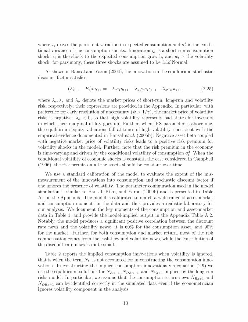
where xt drives the persistent variation in expected consumption and σ2t is the condi-

tional variance of the consumption shocks. Innovation ηt is a short-run consumptionshock, ǫt is the shock to the expected consumption growth, and wt is the volatilityshock; for parsimony, these three shocks are assumed to be i.i.d Normal.

As shown in Bansal and Yaron (2004), the innovation in the equilibrium stochasticdiscount factor satisfies,

(Et+1 − Et)mt+1 = −λcσtηt+1 − λxϕeσtǫt+1 − λσσwwt+1, (2.25)

where λc, λx and λσ denote the market prices of short-run, long-run and volatilityrisk, respectively; their expressions are provided in the Appendix. In particular, withpreference for early resolution of uncertainty (ψ > 1/γ), the market price of volatilityrisks is negative: λσ < 0, so that high volatility represents bad states for investorsin which their marginal utility goes up. Further, when IES parameter is above one,the equilibrium equity valuations fall at times of high volatility, consistent with theempirical evidence documented in Bansal et al. (2005b). Negative asset beta coupledwith negative market price of volatility risks leads to a positive risk premium forvolatility shocks in the model. Further, note that the risk premium in the economyis time-varying and driven by the conditional volatility of consumption σ2

t . When theconditional volatility of economic shocks is constant, the case considered in Campbell(1996), the risk premia on all the assets should be constant over time.

We use a standard calibration of the model to evaluate the extent of the mis-measurement of the innovations into consumption and stochastic discount factor ifone ignores the presence of volatility. The parameter configuration used in the modelsimulation is similar to Bansal, Kiku, and Yaron (2009b) and is presented in TableA.1 in the Appendix. The model is calibrated to match a wide range of asset-marketand consumption moments in the data and thus provides a realistic laboratory forour analysis. We document the key moments of the consumption and asset-marketdata in Table 1, and provide the model-implied output in the Appendix Table A.2.Notably, the model produces a significant positive correlation between the discountrate news and the volatility news: it is 60% for the consumption asset, and 90%for the market. Further, for both consumption and market return, most of the riskcompensation comes from the cash-flow and volatility news, while the contribution ofthe discount rate news is quite small.

Table 2 reports the implied consumption innovations when volatility is ignored,that is when the term NV is not accounted for in constructing the consumption inno-vations. In constructing the implied consumption innovations via equation (2.9) weuse the equilibrium solutions for NR,t+1, NDR,t+1, and NV,t+1 implied by the long-runrisks model. In particular, we assume that the consumption return news NR,t+1 andNDR,t+1 can be identified correctly in the simulated data even if the econometricianignores volatility component in the analysis.

10

The top panel of Table 2 shows that when IES is not equal to one, the impliedconsumption innovations are distorted. In particular, when IES is equal to two, thevolatility of consumption innovations is about twice that of the true consumptioninnovations, and the correlation between the true consumption shock and the impliedconsumption shock is only 50%. Similar distortions are present when the IES is lessthan one. In the bottom panel of Table 2 we report the implications of ignoringvolatility for the stochastic discount factor. When volatility is ignored, for all valuesof the IES the SDF’s volatility is downward biased by about one-third. The marketrisk premium is almost half that of the true one, and the correlations of the SDF withthe return, discount rate, and cash-flow news are distorted. Finally, it is important tonote that even when the IES is equal to one, the SDF is still misspecified. In all, theevidence clearly demonstrates the potential pitfalls that might arise in interpretingasset pricing models and the asset markets sources of risks if the volatility channel isignored.

The analysis above assumed the researcher has access to the return on wealth,rc,t+1. In many instances, however, that is not the case (e.g., Campbell and Vuolteenaho(2004), Campbell (1996)) and the return on the market rd,t+1 is utilized instead. Thefact the market return is a levered asset relative to the consumption/wealth returnexacerbate the inference problems shown earlier. In particular, Table A.3 in theAppendix shows that when the IES is equal to two, the volatility of the implied con-sumption shocks is about 14.3%, relative to the true volatility of only 2.5%. Campbell(1996) (Table 9) reports the implied consumption innovations based on equation (2.9)when volatility is ignored and the return and discount rate shocks are read off a VARusing observed financial data. The volatility of the consumption innovations whenthe IES is assumed to be 2 is about 22%, not far from the quantity displayed in oursimulated model in Table A.3.5 As in our case, lower IES values lead to somewhatsmoother implied consumption innovations. While Campbell (1996) concludes thatthis evidence is more consistent with a low IES, the analysis here suggests that infact this evidence is consistent with an environment in which the IES is greater thanone and the innovation structure contains a volatility component.

3 Volatility, Aggregate Wealth and Consumption

In this section we develop and implement a volatility-based permanent income hy-pothesis framework to quantify the role of the volatility channel for the asset markets.As the aggregate consumption return (i.e., aggregate wealth return) is not directlyobserved in the data we assume that it is a weighted combination of the return tothe stock market and human capital. This allows us to adopt a standard VAR-based

5The data used in Campbell (1996) is from 1890-1990 which leads to slightly higher volatilitynumbers than the calibrated model produces.

11

methodology to extract the innovations to consumption return, volatility, SDF, andassess the importance of the volatility channel for returns to human capital and equity.

3.1 Econometric Specification

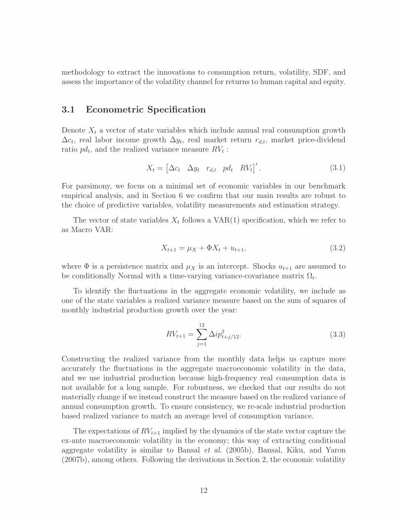
Denote Xt a vector of state variables which include annual real consumption growth∆ct, real labor income growth ∆yt, real market return rd,t, market price-dividendratio pdt, and the realized variance measure RVt :

Xt =[∆ct ∆yt rd,t pdt RVt

]′

. (3.1)

For parsimony, we focus on a minimal set of economic variables in our benchmarkempirical analysis, and in Section 6 we confirm that our main results are robust tothe choice of predictive variables, volatility measurements and estimation strategy.

The vector of state variables Xt follows a VAR(1) specification, which we refer toas Macro VAR:

Xt+1 = µX + ΦXt + ut+1, (3.2)

where Φ is a persistence matrix and µX is an intercept. Shocks ut+1 are assumed tobe conditionally Normal with a time-varying variance-covariance matrix Ωt.

To identify the fluctuations in the aggregate economic volatility, we include asone of the state variables a realized variance measure based on the sum of squares ofmonthly industrial production growth over the year:

RVt+1 =

12∑

j=1

∆ip2t+j/12. (3.3)

Constructing the realized variance from the monthly data helps us capture moreaccurately the fluctuations in the aggregate macroeconomic volatility in the data,and we use industrial production because high-frequency real consumption data isnot available for a long sample. For robustness, we checked that our results do notmaterially change if we instead construct the measure based on the realized variance ofannual consumption growth. To ensure consistency, we re-scale industrial productionbased realized variance to match an average level of consumption variance.

The expectations of RVt+1 implied by the dynamics of the state vector capture theex-ante macroeconomic volatility in the economy; this way of extracting conditionalaggregate volatility is similar to Bansal et al. (2005b), Bansal, Kiku, and Yaron(2007b), among others. Following the derivations in Section 2, the economic volatility

12

Vt then becomes be proportional to the ex-ante expectation of the realized varianceRVt+1 based on the VAR(1):

Vt = V0 +1

2χ(1 − γ)2EtRVt+1

= V0 +1

2χ(1 − γ)2i′vΦXt,

(3.4)

where V0 is an unimportant constant which disappears in the expressions for shocks,iv is a column vector which picks out the realized variance measure from Xt, and χis a parameter which captures the link between the observed aggregate consumptionvolatility and Vt. In the model with volatility risks, we fix the value of χ to the ratioof the variances of the cash-flow to immediate consumption news, consistent withthe theoretical restriction in Section 2. In the specification where volatility risks areabsent, the parameter χ is set to zero.

Following the above derivations, the revisions in future expectations of the eco-nomic volatility can be calculated in the following way:

NV,t+1 =1

2χ(1 − γ)2i′v(I +Q)ut+1, (3.5)

where Q is the matrix of the long-run responses, Q = κ1Φ (I − κ1Φ)−1 .

The VAR specification implies that shocks into immediate market return, NdR,t+1,

and future market discount rate news, NdDR,t+1, are given by6

NdR,t+1 = i′rut+1, Nd

DR,t+1 = i′rQut+1, (3.6)

where ir is a column vector which picks out market return component from the setof state variables Xt.

While the market return is directly observed and the market return news canbe extracted directly from the VAR(1), in the data we can only observe the laborincome but not the total return to human capital. We make the following identifyingassumption, identical to Lustig and Van Nieuwerburgh (2008), that expected laborincome return is linear in the state variables:

Etry,t+1 = α + b′Xt, (3.7)

where b captures the loadings of expected human capital return to the economicstate variables. Given this restriction, the news into future discounted human capitalreturns, Ny

DR,t+1, is given by,

NyDR,t+1 = b′Φ−1Qut+1, (3.8)

6In what follows, we use superscript ”d” to denote shocks to the market return, and superscript”y” to identify shocks to the human capital return. Shocks without the superscript refer to theconsumption asset, consistent with the notations in Section 2.

13

and the immediate shock to labor income return, NyR,t+1, can be computed as follows:

NyR,t+1 = (Et+1 − Et)

(∞∑

j=0

κj1∆yt+j+1

)−Ny

DR,t+1

= i′y(I +Q)ut+1 − b′Φ−1Qut+1,

(3.9)

where the column vector iy picks out labor income growth from the state vector Xt.

To construct the aggregate consumption return (i.e.,aggregate wealth return), wefollow Jagannathan and Wang (1996), Campbell (1996), Lettau and Ludvigson (2001)and Lustig and Van Nieuwerburgh (2008) and assume that it is a portfolio of thereturns to the stock market and returns to human capital:

rc,t = (1 − ω)rd,t + ωry,t. (3.10)

The share of human wealth in total wealth ω is assumed to be constant. It imme-diately follows that the immediate and future discount rate news on the consumptionasset are equal to the weighted average of the corresponding news to the humancapital and market return, with a weight parameter ω :

NR,t+1 = (1 − ω)NdR,t+1 + ωNy

R,t+1,

NDR,t+1 = (1 − ω)NdDR,t+1 + ωNy

DR,t+1.(3.11)

These consumption return innovations can be expressed in terms of the VAR(1) pa-rameters and shocks and the vector of the expected labor return loadings b followingEquations (3.6)-(3.9).

Finally, we can combine the expressions for the volatility news, immediate anddiscount rate news on the consumption asset to back out the implied immediateconsumption shock following the Equation (2.9):

ct+1 − Etct+1 = NR,t+1 + (1 − ψ)NDR,t+1 +ψ − 1

γ − 1NV,t+1

=[(1 − ω)i′rQ+ ω(i′y(I +Q) − b′Φ−1Q)

]ut+1︸ ︷︷ ︸

NR,t+1

+ (1 − ψ)[(1 − ω)i′rQ+ ωb′Φ−1Q

]ut+1︸ ︷︷ ︸

NDR,t+1

+

(ψ − 1

γ − 1

)1

2χ(1 − γ)2i′vQut+1

︸ ︷︷ ︸NV,t+1

≡ q(b)′ut+1.

(3.12)

The vector q(b) defined above depends on the model parameters, and in particular,it depends linearly on the expected labor return loadings b. On the other hand, as

14

consumption growth itself is one of the state variables in Xt, it follows that theconsumption innovation satisfies,

ct+1 −Etct+1 = i′cut+1, (3.13)

where ic is a column vector which picks out consumption growth out of the statevector Xt. We impose this important consistency requirement that the model-impliedconsumption shock in Equation (3.12) matches the VAR consumption shock in (3.13),so that

q(b) ≡ ic, (3.14)

and solve the above equation, which is linear in b, to back out the unique expectedhuman capital return loadings b. That is, in our approach the specification for theexpected labor return ensures that the consumption innovation implied by the modelis identical to the consumption innovation in the data.

3.2 Data and Estimation

In our empirical analysis, we use an annual sample from 1930 to 2010. Real consump-tion corresponds to real per capita expenditures on non-durable goods and services,and real income is the real per capita disposable personal income; both series aretaken from the Bureau of Economic Analysis. Market return data is for a broad port-folio from CRSP. The summary statistics for these variables are presented in Table1. The average labor income and consumption growth rates are about 2%. The laborincome is more volatile than consumption growth, but the two series co-move quiteclosely in the data with the correlation coefficient of 0.80. The average log marketreturn is 5.7%, and its volatility is almost 20%. The realized consumption variance isquite volatile in the data, and spikes up considerably in the recessions. Notably, therealized variance is negatively correlated with the price-dividend ratio: the correla-tion coefficient is about -0.25, so that asset prices fall at times of high macroeconomicvolatility, consistent with findings in Bansal et al. (2005b).

We estimate the Macro VAR specification in (3.2) using equation-by-equationOLS. For robustness, we also consider an MLE approach where we incorporate theinformation in the conditional variance of the residuals; the results are very similar,and are discussed in the robustness section. To derive the implications for the market,human capital, and wealth portfolio returns, we set the risk aversion coefficient γ to5 and the IES parameter ψ to 2. The share of human wealth in the overall wealthω is set to 0.8, the average value used in Lustig and Van Nieuwerburgh (2008). Inthe full model specification featuring volatility risks we fix the volatility parameter χaccording to the restriction in Equation (2.18). To discuss the model implications inthe absence of volatility risks, we set χ equal to zero.

15

The Macro VAR estimation results are reported in Table 3. The magnitudes of R2

in the regressions vary from 10% for the market return to 80% for the price-dividendratio. Notably, the consumption and labor income growth rates are quite predictablewith this rich setting, with the R2 of 60% and nearly 40%, respectively. Because of thecorrelation between the variables, it is hard to interpret individual slope coefficientsin the regression. Note, however, that the ex-ante consumption volatility is quitepersistent with an autocorrelation coefficient of 0.63 on annual frequency, and itloads significantly and negatively on the market price-dividend ratio. 7

We plot the ex-ante consumption volatility and the expected consumption growthrate on Figure 2. The evidence on persistent fluctuations in the ex-ante macroeco-nomic volatility and the gradual decline in the volatility over time is similar to thefindings in Stock and Watson (2002) and McConnell and Perez-Quiros (2000). No-tably, the volatility process is strongly counter-cyclical: its correlation with the NBERrecession indicator is -40%, and it is -30% with the expected real consumption growth.Consistent with this evidence, the news in future expected consumption implied bythe Macro VAR, NECF , is sharply negative at times of high volatility. Indeed, asshown in Table 4, future expected consumption news are on average -1.70% at timesof high (top 25%) versus 2.23% in low (bottom 25%) volatility times. Further, inFigure 2 we plot a Macro VAR impulse response of consumption growth to one stan-dard deviation shock in ex-ante consumption volatility, V art∆ct+1; see Appendix forthe details of the computations. One standard deviation volatility shock correspondsto an increase in ex-ante consumption variance by (1.95%)2. As shown in the Figure,consumption growth significantly declines by almost 1% on the impact of volatilitynews and remains negative up to five years in the future. The response of the laborincome growth is similar.

In the full model with volatility risks, the volatility news is strongly correlatedwith the discount rate news in the data. As documented in Table 4, the correlationbetween the volatility news and the discount rate news on the market reaches nearly90%, and the correlations of the volatility news with the discount rate news to laborreturn and the wealth portfolio are 30% and 80%, respectively. A high correlationbetween the volatility news and the discount rate news to the wealth return is evidenton Figure 4. These findings are consistent with the intuition of the economic long-run risks model where a significant component of the discount rate news is drivenby shocks to consumption volatility (see Section 2.3). On the other hand, when thevolatility risks are absent, the discount rate news no longer reflect the fluctuations inthe volatility, but rather mirror the revisions in future expectations of consumption.As a result, the correlation of the implied discount rate news with volatility newsbecomes -0.85 for the labor return, and -0.3 for the wealth portfolio. The implieddiscount rate news ignoring volatility risks is very different from the discount ratenews when volatility risks are taken into account. For example, when volatility risks

7The process for realized volatility is obviously more volatile and less persistent.

16

are accounted for, the measured discount rate news is 5.14% in the latest recessionof 2008 and 0.91% in 2001. Without the volatility channel, however, it would appearthat the discount rate news is negative at those times: the measured discount rateshock is -2.86% in 2008 and -0.73% in 2001. Thus, ignoring the volatility channel,the discount rate on the wealth portfolio can be significantly mis-specified due tothe omission of the volatility risk component, which would alter the dynamics of theaggregate returns as we discuss in subsequent section.

3.3 Labor, Market and Wealth Return Dynamics

Table 5 reports the evidence on correlations between immediate and future returns onthe market, human capital and wealth portfolio. Without the volatility risk channel,shocks to the market and human capital returns are significantly negatively correlated,which is consistent with the evidence in Lustig and Van Nieuwerburgh (2008). Indeed,as shown in the top panel of the Table, the correlations between immediate stockmarket and labor income return news, Nd

R,t+1 and NyR,t+1, the discount rate news,

NdDR,t+1 and Ny

DR,t+1, and the future long-term (5-year) expected returns, Etrdt→t+5

and Etryt→t+5, range between -0.50 and -0.70. All these correlations turn positive when

the volatility channel is present: the correlation of immediate return news increasesto 0.20; and for discount rates and the expected 5-year returns it goes up to 0.25and 0.40, respectively. Figure 3 plots the implied time-series of long-term expectedreturns on the market and human capital. A negative correlation between the twoseries is evident in the model specification which ignores volatility risks. The evidencefor the co-movements of returns is similar for the wealth and human capital, and themarket and wealth portfolios, as shown in the middle and lower panels of Table 5.Because the wealth return is a weighted average of the market and human capitalreturns, these correlations are in fact positive without the volatility channel. Thesecorrelations increase considerably and become closer to one once the volatility risksare introduced. For example, the correlations between immediate and future expectednews on the market and wealth returns rise to 80% with the volatility risk channel,while without volatility risks the correlation is 0.07 for the discount rates, 0.26 forthe 5-year expected returns and 0.46 for the immediate return shocks.

To understand the role of the volatility risks for the properties of the wealthportfolio, consider again the consumption equation in (2.12), which for conveniencewe reproduce below:

(Et+1 − Et)

(∞∑

j=1

κj1∆ct+j+1

)

= ψNDR,t+1 −ψ − 1

γ − 1NV,t+1

= ψ(ωNy

DR,t+1 + (1 − ω)NdDR,t+1

)−ψ − 1

γ − 1NV,t+1

(3.15)

17

When the volatility risks are not accounted for, Nv = 0 and all the variation in thefuture cash flows is driven by news to discount rates on the market and the humancapital. However, as shown in Table 4, in the data consumption growth is muchsmoother than asset returns: the volatility of cash-flow news is about 5% relative to14% for the discount rate news on the market. Hence, to explain relatively smoothvariation in cash flows in the absence of volatility news, the discount rate news tohuman capital must offset a large portion of the discount rate news on the market,which manifests as a large negative correlation between the two returns documentedin Table 5. On the other hand, when volatility news is accounted for, they removethe risk premia fluctuations from the discount rates and isolate the news in expectedcash flows. Indeed, a strong positive correlation between volatility news and discountrate news in the data is evident in Table 4. This allows the model to explain thelink between consumption and asset markets without forcing a negative correlationbetween labor and market returns.

We use the extracted news components to identify the innovation into the stochas-tic discount factor, according to Equation (2.15), and document the implications forthe risk premia in Table 6. At our calibrated preference parameters, in the modelwith volatility risks the risk premium on the market is 7.2%; it is 2.6% for the wealthportfolio, and 1.4% for the labor return. Most of the risk premium comes from thecash-flow and volatility risks, and the volatility risks contribute about one-half to theoverall risk premia. The discount rate shocks contribute virtually nothing to the riskpremia. These findings are consistent with the economic long-run risks model (seeTable A.2). Without the volatility channel, the risk premia are 2.3% for the market,0.9% for the wealth return and 0.5% for the labor return.

While the main results in the paper are obtained with preference parameters γ = 5and ψ = 2, in Table 7 we document the model implications for a range of the IES pa-rameter from 0.5 to 3.0. Without the volatility channel, the correlations between laborand market returns are negative and large at all considered values for the preferenceparameters, which is consistent with the evidence in Lustig and Van Nieuwerburgh(2008). In the model with volatility risks, one requires IES sufficiently above oneto generate a positive link between labor and market returns – with IES below one,the volatility component no longer offsets risk premia variation in the consumptionequation, which makes the labor-market return correlations even lower than in thecase without volatility risks. The evidence is similar for other values of risk aversionparameter. Higher values for risk aversion lead to higher risk premium, that is whywe chose moderate values of γ in our analysis.

18

4 Volatility-Based Dynamic CAPM

To further highlight the importance of volatility risks for understanding the dynamicsof asset prices, we use a market-based VAR approach to news decomposition. As fre-quently done in the literature, here, we assume that the wealth portfolio correspondsto the aggregate stock market and, therefore, is observable. This assumption allowsus to measure cash-flow, discount-rate and volatility news directly from the availablestock market data. As shown in Section 3, in a more general setting that explicitlymakes a distinction between aggregate and financial wealth and accounts for time-variation in volatility, realized and expected returns on wealth and stock market arehighly correlated. This evidence suggests that we should be able to learn about time-series dynamics of fundamental risks and their prices from the observed equity data.Furthermore, to sharpen identification of underlying risks, we will extract them byexploiting both time-series and cross-sectional moment restrictions.

The theoretical framework here is same as the one in Section 2 with the returnon the consumption asset equal to the return on the market portfolio. Hence, theequilibrium risk premium on any asset is determined by its exposure to the innova-tion in the market return and news about future discount rates and future volatility.The multi-beta implication of our model is similar to the multi-beta pricing of the in-tertemporal CAPM of Merton (1973) where the risk premium depends on the marketbeta and the asset exposure to state variables that capture changes in future invest-ment opportunities. What distinguishes our volatility-based dynamic capital assetpricing model (DCAPM) from the Merton’s framework is that, in our model, bothrelevant risk factors and their prices are identified and pinned down by the underlyingmodel primitives and preferences. This is important from an empirical perspective asit provides us with testable implications that can be taken to the data. Note also thatin our volatility-based DCAPM, derived from recursive preferences, the relevant eco-nomic risks comprise not only short-run fluctuations (as in the equilibrium C-CAPMof Breeden (1979)) but also risks that matter in the long run.

4.1 Market-Based Setup

As derived above, the stochastic discount rate of the economy is given by:

mt+1 − Etmt+1 = −γNCF,t+1 +NDR,t+1 +NV,t+1. (4.1)

In order to measure news components from equity data, we assume that the state ofthe economy is described by vector:

Xt ≡ (RVr,t, zt, ∆dt, tst, dst, it)′ ,

where RVr,t is the realized variance of the aggregate market portfolio; zt is the logof the market price-dividend ratio; ∆dt is the continuously compounded dividend

19

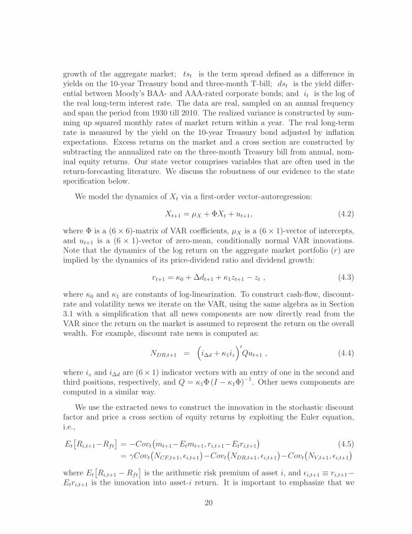
growth of the aggregate market; tst is the term spread defined as a difference inyields on the 10-year Treasury bond and three-month T-bill; dst is the yield differ-ential between Moody’s BAA- and AAA-rated corporate bonds; and it is the log ofthe real long-term interest rate. The data are real, sampled on an annual frequencyand span the period from 1930 till 2010. The realized variance is constructed by sum-ming up squared monthly rates of market return within a year. The real long-termrate is measured by the yield on the 10-year Treasury bond adjusted by inflationexpectations. Excess returns on the market and a cross section are constructed bysubtracting the annualized rate on the three-month Treasury bill from annual, nom-inal equity returns. Our state vector comprises variables that are often used in thereturn-forecasting literature. We discuss the robustness of our evidence to the statespecification below.

We model the dynamics of Xt via a first-order vector-autoregression:

Xt+1 = µX + ΦXt + ut+1, (4.2)

where Φ is a (6 × 6)-matrix of VAR coefficients, µX is a (6 × 1)-vector of intercepts,and ut+1 is a (6 × 1)-vector of zero-mean, conditionally normal VAR innovations.Note that the dynamics of the log return on the aggregate market portfolio (r) areimplied by the dynamics of its price-dividend ratio and dividend growth:

rt+1 = κ0 + ∆dt+1 + κ1zt+1 − zt , (4.3)

where κ0 and κ1 are constants of log-linearization. To construct cash-flow, discount-rate and volatility news we iterate on the VAR, using the same algebra as in Section3.1 with a simplification that all news components are now directly read from theVAR since the return on the market is assumed to represent the return on the overallwealth. For example, discount rate news is computed as:

NDR,t+1 =(i∆d + κ1iz

)′

Qut+1 , (4.4)

where iz and i∆d are (6× 1) indicator vectors with an entry of one in the second andthird positions, respectively, and Q = κ1Φ (I − κ1Φ)−1. Other news components arecomputed in a similar way.

We use the extracted news to construct the innovation in the stochastic discountfactor and price a cross section of equity returns by exploiting the Euler equation,i.e.,

Et[Ri,t+1−Rft

]= −Covt

(mt+1−Etmt+1, ri,t+1−Etri,t+1

)(4.5)

= γCovt(NCF,t+1, ǫi,t+1

)−Covt

(NDR,t+1, ǫi,t+1

)−Covt

(NV,t+1, ǫi,t+1

)

where Et[Ri,t+1 − Rft

]is the arithmetic risk premium of asset i, and ǫi,t+1 ≡ ri,t+1−

Etri,t+1 is the innovation into asset-i return. It is important to emphasize that we

20

carry out estimation under the null of the model. In particular, we restrict thepremium of a zero-beta asset and impose the model’s restrictions on the market pricesof discount-rate and volatility risks. The price of cash-flow risks (i.e., risk aversion)is estimated along with time-series parameters of the model.

To extract return innovations for the cross section, we use an econometric approachsimilar to Bansal, Dittmar, and Lundblad (2005a) and Bansal, Dittmar, and Kiku(2009a) that allows for a sharper identification of long-run cash-flow risks in assetreturns. In particular, for each equity portfolio, we estimate its long-run cash-flowexposure (φi) by regressing portfolio’s dividend growth rate on the three-year movingaverage of the market dividend growth:

∆di,t = µi + φi∆dt−2→t + ǫdi,t , (4.6)

where ∆di,t is portfolio-i dividend growth, ∆dt−2→t is the average growth in marketdividends from time t − 2 to t, and ǫdi,t denotes idiosyncratic portfolio news. Usingthe log-linearization of return:

ri,t+1 = κi,0 + ∆di,t+1 + κi,1zi,t+1 − zi,t , (4.7)

the innovation into asset-i return is then given by:

ǫi,t+1 = φi(∆dt+1 − Et∆dt+1) + ǫdi,t+1 + κiǫzi,t+1 , (4.8)

where zi,t is the price-dividend ratio of portfolio i, κi,0 and κi,1 are portfolio-specificconstants of log-linearization, (∆dt+1 − Et∆dt+1) is the VAR-based innovation inthe market dividend growth rate, and ǫzi,t+1 is the innovation in the portfolio price-dividend ratio obtained by regressing zi,t+1 on the VAR state variables. We use theextracted innovation in the portfolio return to construct the risk-premium restrictiongiven in Equation (4.5).8

To extract news and construct the innovation in the stochastic discount factor,we estimate time-series parameters and the coefficient of risk aversion using GMM byexploiting two sets of moment restrictions. The first set of moments comprises theVAR orthogonality moments; the second set contains the Euler equation restrictionsfor the market portfolio and a cross-section of five book-to-market and five size sortedportfolios. To ensure that the moment conditions are scaled appropriately, we weighteach moment by the inverse of its variance and allow the weights to be continuouslyup-dated throughout estimation. Further details of the GMM estimation are providedin Appendix C.

8Our empirical results remain similar if instead we rely on the cointegration-based specificationof Bansal et al. (2009a).

21

4.2 Ex-Ante Volatility and Discount-Rate Dynamics

The GMM estimates of the market-based VAR dynamics are presented in Table 8.As shown in the first row of the table, the realized variance of the market returnis highly predictable with an R2 of more than 60%. Time-variation in the one-yearahead expected variance is coming mostly from variation in realized variance, termand default spreads, and the risk-free rate, all of which are quite persistent in thedata. The conditional variance, therefore, features persistent time-series dynamicswith a first-order autocorrelation coefficient of about 0.69. These persistent dynam-ics are consistent with empirical evidence of low-frequency fluctuations in marketvolatility documented in the literature (see, for example, Bollerslev and Mikkelsen(1996) among others).

We find that the extracted discount-rate and volatility risks are strongly counter-cyclical and positively correlated. Both news tend to increase during recessions anddecline during economic expansions. At the one-year horizon, the correlation betweendiscount-rate and volatility news is 0.47. This evidence aligns well with economicintuition. As the contribution of risk-free rate news is generally small, discount-raterisks are mostly driven by news about future risk premia, and the latter is tied toexpectations about future economic uncertainty. Consequently, discount rates andconditional volatility of the market portfolio share common time-series dynamics,especially at low frequencies. We illustrate their co-movement in Figure 5 by plottingthe 5-year expected market return and the 5-year conditional variance implied by theestimated VAR. As the figure shows, both discount rates and the conditional variancefeature counter-cyclical fluctuations, and almost mirror the dynamics of one another.The correlation between the two time series is 0.75. Motivated by the documentedhigh correlation between discount rates and volatility, in Section 4.4 we consider arestricted version of our volatility-based DCAPM that constraints variations in thediscount rate to variations in the conditional variance.

4.3 Pricing Implications of the Volatility-based DCAPM

The cross-sectional implications of the volatility-based DCAPM are given in Table 9.In this specification, no restrictions are imposed on the dynamics of discount rates.The table presents sample average excess returns of the market portfolio and thecross section, risk premia implied by the market-based model, and asset exposure tocash-flow, discount-rate and volatility risks. The bottom panel of the table shows theestimate of the market price of cash-flow risks. The evidence reported in the tableyields several important insights. First, we find that cash-flow risks play a dominantrole in explaining both the level and the cross-sectional variation in risk premia. Atthe aggregate market level, cash-flow risks account for 4.8% or, in relative terms, forabout 60% of the total risk premium. Cash-flow betas are monotonically increasing

22

in book-to-market characteristics and monotonically declining with size. Value andsmall stocks in the data are more sensitive to persistent cash-flow risks than aregrowth and large firms, which is consistent with the evidence in Bansal et al. (2005a),Hansen, Heaton, and Li (2008) and Bansal et al. (2009a).

Second, we find that all assets have negative exposure to discount-rate and volatil-ity risks. That is, in the data, prices of all equity portfolios tend to fall when discountrates or volatility are expected to be high. Because the prices of discount-rate andvolatility risks, according to the model, are equal to negative one, both risks carrypositive premia. The documented positive compensation for volatility risks is con-sistent with the evidence of a positive variance premium reported in Drechsler andYaron (2011), and Bollerslev, Tauchen, and Zhou (2009). These papers show thatthe estimate of the variance risk premium defined as a difference between expectedvariances under the risk-neutral and physical measure is not only positive on average,it is almost always positive in time series. Our findings are also confirmed by theoption-based evidence in Coval and Shumway (2001) who show that, in the data,average returns on zero-market-beta straddles are significantly negative. Recently,Campbell et al. (2011) also consider an ICAPM framework with time-varying volatil-ity. They, however, report a negative compensation for volatility risks which conflictswith the discussed evidence on the variance risk premium and expected straddle re-turns. From an economic standpoint, high volatility states are states of low prices andlow aggregate wealth. Hence, volatility risks should carry a positive risk premium.

The evidence in Table 9 also shows that discount-rate and volatility risks, each,account for about 20% of the overall market risk premium, and seem to affect thecross section of book-to-market sorted portfolios in a similar way. Both discount-rateand volatility risks matter more for the valuation of growth firms than that of valuefirms. This is consistent with economic intuition that growth firms, whose cash flowsare shifted to the future, are more exposed to risk-premia and discount-rate variation.

Overall, our volatility-based DCAPM accounts for about 96% of the cross-sectionalvariation in risk premia, and implies a value premium of 6.1% and a size premiumof about 6.8%. The cross-sectional fit of the model is illustrated in Figure 6(a). Theestimate of the market price of cash-flow risks is statistically significant: γ = 2.64(SE=0.41), and the model is not rejected by the overidentifying restrictions: the χ2

test statistic is equal to 7.74 with a p-value of 0.65.

Our empirical evidence is fairly robust to economically reasonable changes in theVAR specification, sample period or frequency of the data. For example, omittingterm and default spreads from the VAR yields a p-value of 0.25. The estimation ofthe model using post-1964 quarterly-sampled data results in a χ2 statistic of 8.1 witha corresponding p-value of 0.33. Across these alternative specifications, the estimatesof the market price of cash-flow risks continue to be significant, and the extracteddiscount-rate and volatility risks remain strongly positively correlated.

23

4.4 Asset Pricing Implications of the Restricted DCAPM

In addition to the unrestricted model discussed above, we consider a specification thatties the dynamics of the expected return of the market portfolio to the dynamics of itsconditional variance. This restricted specification has the advantage of allowing for abetter identification of the role of volatility risks and is motivated by a documentedtight link between discount-rate and volatility news. The estimation details of thisset-up are presented in Appendix D.

Table 10 presents the asset pricing implications of the restricted volatility-basedDCAPM that incorporates the constraint on the dynamics of the risk premium. Itreports the model-implied premia of the aggregate market and the cross section,and portfolio betas with respect to each risk source. Consistent with the evidencefrom the unrestricted model, cash-flow risks remain the key determinant of the levelof the risk premium and its dispersion in the cross section. Still, volatility riskscontribute significantly. At the aggregate level, about 2% of the premium is due tovolatility risks. Thus, volatility risks account for about 25% of the overall marketpremium. At the cross-sectional level, the contribution of volatility risks is fairlyuniform across size-sorted portfolios, but displays some tangible heterogeneity in thebook-to-market sort. Value firms in the data seem to be quite immune to volatilityrisks, and therefore carry an almost zero volatility risk premium. Growth firms, on theother hand, are relatively sensitive to news about future economic uncertainty. Therestricted specification is not rejected by the test of overidentifying restrictions and,as shown in Figure 6(b), accounts for a large portion of the cross-sectional variationin risk premia. Once again notice that all equity portfolios have negative exposure tovolatility risks, and therefore, provide investors with positive volatility premia.

The variance decomposition of the stochastic discount factor reveals that 52% ofthe overall variation in the SDF is due to cash-flow risks and about 12% is due tovolatility risks. While the direct contribution of volatility risks may seem modest,they account for another 32% of the variation in the SDF through their covariationwith cash-flow news. Similar to the consumption-based evidence presented in Section3, cash-flow news rises during expansions and falls in recessions, while news aboutfuture uncertainty exhibits strongly counter-cyclical dynamics. Volatility risks havea sizable effect on the dynamics of asset prices. A one-standard deviation increasein volatility news leads to a negative 11% fall in the return of the aggregate marketportfolio.

To summarize, our empirical evidence in Section 4 highlights the importance ofvolatility risks for understanding the cross-sectional risk-return tradeoff. We showthat revisions in expectations about future volatility contribute significantly to theoverall variation in the stochastic discount factor. In the data, equity prices fall whenvolatility news and marginal utility are high. Therefore, volatility risks carry a sizableand positive risk premium.

24

5 Robustness

We conduct a number of robustness checks to ensure that our main results are notsensitive to volatility measurements, choice of the predictive variables and estima-tion strategy. In our benchmark Macro VAR specification, we measure the realizedvariance using squared monthly industrial production growth rates, scaled to matchthe overall consumption volatility. First, we check that our results remain broadlysimilar if we instead compute the realized variance based on the square of the annualconsumption growth; in this case, the implied correlations between immediate newsto the stock market and labor return is 0.20; it is 0.03 for the discount rate news and0.26 for the 5-year expected returns. Second, we confirm that adding other predictivevariables into the VAR(1) does not materially change our results, either. For exam-ple, if we include the data on interest rate, slope of the term structure and defaultspread into our benchmark Macro VAR specification, the implied correlations be-tween human capital and market return are all in 0.2-0.4 range. Finally, we consideran alternative MLE estimation strategy where we allow the variance of the VAR(1)residuals of consumption and income growth to be time-varying and driven by theex-ante volatility variable. The results are very similar to our benchmark Macro VAR:the correlations between human capital and market returns are positive and rangebetween 5% for the immediate news to 45% for the 5-year expected returns.

In Section 4 we assume that the volatility of volatility shocks is constant. Toconfirm robustness of our DCAPM evidence, we estimate a more general set-up thatallows for time-variation in the variance of volatility shocks. In particular, we as-sume that state vector Xt follows the first-order dynamics as in Equation (4.2), withut+1 ∼ N(0, σr,tΩ), and σr,t = V art(NR,t+1). Here, we assume that all time-variationin conditional second moments of the VAR innovations (including the innovation tothe variance component) is driven by a single state variable.9 We maintain the as-sumption that the conditional risk premia are proportional to the conditional varianceof the return of the market portfolio.10 One can show that in this set-up, the dynamicsof the aggregate volatility component Vt are given by:

Vt ≈ V0 + ξσ2r,t , (5.1)

where ξ is a non-liner function of the underlying preference and time-series parame-ters.

We find that the asset pricing implications of this generalized DCAPM set-up arecomparable to the ones in our benchmark specification. Consistent with the evidencediscussed above, cash-flow risks play a dominant role in explaining the cross-sectionalrisk-return tradeoff. The contribution of volatility risks remains significant and, in

9The estimation is carried out by imposing positivity restriction on σr,t.10Empirical evidence is robust if the assumption on the dynamics of risk premia is relaxed.

25

fact, is slightly larger relative to the case when volatility shocks are homoscedastic.On average, volatility risks account for about 25% of the overall risk premia in thecross-section, and about 40% of the total premium of the market portfolio. Thecontribution of volatility risks varies significantly across stocks sorted on book-to-market characteristic. Similar to the implications of our benchmark specification,growth stocks are more sensitive to volatility (and discount rate) variation than valuestocks are.

Conclusions

In this paper we show that volatility news is an important source of risk that affectsthe measurement and interpretation of underlying risks in the economy and finan-cial markets. Our theoretical analysis yields a dynamics asset pricing model withthree sources of risks: cash-flow, discount-rate and volatility risks, each carrying aseparate risk premium. We show that ignoring volatility risks may lead to sizablemis-specifications of the dynamics of the stochastic discount factor and equilibriumconsumption, and distorted inferences about risk and return. Calibrating an off-the-shelf, long-run risks model, we find that potential distortions caused by neglectingtime-variation in economic volatility are indeed significant and manifest in large up-ward biases in the volatility of consumption news and large downward biases in thevolatility of the implied stochastic discount factor and, consequently, risk premia.

Consistent with the existing empirical evidence, we document that both macro-economic and return-based measures of volatility are highly persistent. Importantly,we also find that, in the data, a rise in volatility is typically accompanied by asignificant decline in realized and expected consumption, a fall in equity prices and anincrease in risk premia. That is, high volatility states are states of high risk reinforcedby low economic growth and high discount rates. This evidence is consistent withthe equilibrium relationship among volatility, consumption and asset prices impliedby our model. A specification that ignores time-variation in volatility, in contrast tothe data, would imply an upward revision in expected lifetime consumption followingan increase in discount rates and would clearly fail to account for a strong positivecorrelation between volatility and discount-rate risks.

The empirical evidence we present highlights the importance of volatility risks forthe joint dynamics of human capital and equity returns, and the cross-sectional risk-risk tradeoff. Our dynamic volatility-based asset pricing model is able to reverse thepuzzling negative correlation between equity and human-capital returns documentedpreviously in the literature in the context of a homoscedastic economy. By incorpo-rating empirically robust positive relationship between ex-ante volatility and discountrates (a missing link in the homoscedastic case), our model implies a positive corre-lation between returns to human capital and equity while, simultaneously, matching

26

time-series dynamics of aggregate consumption. We also show that quantitatively,volatility risks help explain both the level and variation in risk premia across port-folios sorted on size and book-to-market characteristics. We find that during timesof high volatility in financial markets (hence, high marginal utility), equity portfoliostend to realize low returns. Therefore, equity markets carry a positive premium forvolatility risk exposure.

27

A Long-Run Risks Model Setup

In a standard long-run risks model of Bansal and Yaron (2004), consumption dynamicssatisfies

∆ct+1 = µ+ xt + σtηt+1, (A.1)

∆dt+1 = µd + φxt + πσtηt+1 + ϕdσtud,t+1, (A.2)

xt+1 = ρxt + ϕeσtǫt+1, (A.3)

σ2t+1 = σ2

c + ν(σ2t − σ2

c ) + σwwt+1, (A.4)

where ρ governs the persistence of expected consumption growth xt, and ν determines thepersistence of the conditional aggregate volatility σ2

t . ηt is a short-run consumption shock,ǫt is the shock to the expected consumption growth, and wt+1 is the shock to the conditionalvolatility of consumption growth; for parsimony, these three shocks are assumed to be i.i.d

Normal.

The equilibrium solution to the price-consumption ratio, pct, is linear in the expectedgrowth and consumption volatility:

pct = A0 +Axxt +Aσσ2t , (A.5)

where the equilibrium price-to-consumption ratio parameters satisfy

Ax =1 − 1

ψ

1 − κ1ρ, Aσ = (1 − γ)(1 −

1

ψ)

1 +

(κ1ϕx1−κ1ρ

)2

2(1 − κ1ν)

, (A.6)

and κ1 is the log-linearization parameter.

The innovation into the stochastic discount factor is determined by the short-run, ex-pected consumption and volatility shocks:

mt+1 − Etmt+1 = −λcσtηt+1 − λxϕeσtǫt+1 − λσσwwt+1, (A.7)

where the discount rate parameters and market prices of risks satisfy

mx = −1

ψ, mσ = (1 − θ)(1 − κ1ν)Aσ , m0 = θ log δ − γµ− (θ − 1) log κ1 −mσσ

2c ,

λc = γ, λx = (1 − θ)κ1Ax, λσ = (1 − θ)κ1Aσ.

(A.8)

Given the equilibrium model solution, we can provide explicit expressions for the imme-diate consumption returns news, NR,t+1, the discount-rate news, NDR,t+1, and the volatility

28

news, NV,t+1, in terms of the underlying shocks and model parameters. The consumptionreturn shock, NR,t+1 is driven by all three shocks in the economy,

NR,t+1 = Axκ1ϕxσtǫt+1 +Aσκ1σwwt+1 + σtηt+1, (A.9)

while the discount rate news, NDR,t+1 is driven only by the expected growth and volatilityinnovations:

NDR,t+1 =1

ψ

κ1

1 − κ1ρϕeσtǫt+1 − κ1Aσσwwt+1. (A.10)

The economic volatility component, Vt, is directly related to the conditional variance ofconsumption growth:

Vt =1

2V art(rc,t+1 +mt+1) = const+

1

2χ(1 − γ)2σ2

t , (A.11)

where the proportionality coefficient χ satisfies,

χ =

(κ1ϕe

1 − κ1ρ

)2

+ 1. (A.12)

Consistent with our discussion in Section 2, as volatility shocks are homoscedastic andthere is a single consumption volatility factor, the volatility parameter χ is unambiguouslypositive and is equal to the ratio of variances of the long-run cash flows news, NCF,t+1, tothe immediate consumption news, NC,t+1:

χ =V ar(NCF,t+1)

V ar(NC,t+1). (A.13)

The innovation into the future expected volatility NV,t+1 satisfies

NV,t+1 =1

2χ(1 − γ)2

κ1

1 − κ1νσwwt+1. (A.14)

Notice that all the three shocks, NR,t+1, NDR,t+1 and NV,t+1, are correlated with eachother as they depend on the underlying shocks in the economy. In particular, if IES is aboveone, the discount rate shocks and the volatility shocks are positively correlated, because thevolatility is driving the risk premium which is an important component of discount rateinnovations.

The expression for consumption innovations, NC,t+1, and the stochastic discount factorcan now be written in terms of the innovations to the consumption return, discount rateand volatility shocks, as shown in Equations (2.9) and (2.15). Under the null of the model,the consumption shock is equal to σtηt+1, and the innovation into the stochastic discountfactor matches the expression in Equation (A.7).

29

The price-dividend ratio satisfies

pdt = H0 +Hxxt +Hσσ2t , (A.15)

where

Hx =φ− 1

ψ

1 − κ1dρ, Hσ =

ms + 0.5((π − γ)2 + (λx − κ1dHx)2ϕ2

e + ϕ2d)

1 − κ1dν, (A.16)

for a log-linearization parameter κ1d

log κ1d = m0 + µd +Hσσ20(1 − κ1dν) + 0.5(λσ − κ1dHσ)

2σ2w. (A.17)

30

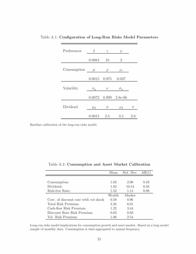
Table A.1: Configuration of Long-Run Risks Model Parameters

Preferences δ γ ψ

0.9984 10 2

Consumption µ ρ ϕe

0.0015 0.975 0.037

Volatility σg ν σw

0.0072 0.999 2.8e-06

Dividend µd φ ϕd π

0.0015 2.5 3.5 2.0

Baseline calibration of the long-run risks model.

Table A.2: Consumption and Asset Market Calibration

Mean Std. Dev. AR(1)

Consumption: 1.82 2.90 0.43Dividend: 1.82 10.54 0.34Risk-free Rate: 1.52 1.14 0.98

Wealth MarketCorr. of discount rate with vol shock 0.59 0.96Total Risk Premium 2.28 6.01Cash-flow Risk Premium 1.22 3.44Discount Rate Risk Premium 0.03 0.03Vol. Risk Premium 1.06 2.54

Long-run risks model implications for consumption growth and asset market. Based on a long modelsample of monthly data. Consumption is time-aggregated to annual frequency.

31

Table A.3: Consumption Innovation Ignoring Volatility and Consumption Return

IES = 2 IES= 1 IES = 0.75Ignore Vol Mkt Vol True Ignore Vol Mkt Vol True Ignore Vol Mkt Vol True

Panel A: Model with Time-varying Volatility

Vol of cons. shock 14.32 12.73 2.49 11.53 10.87 2.49 8.67 8.82 2.49

Corr. with True cons. shock 0.35 0.39 1.00 0.43 0.46 1.00 0.58 0.57 1.00

Panel B: Model with Constant Volatility

Volatility of cons. shock 8.48 8.48 2.49 8.47 8.47 2.49 8.41 8.41 2.49

Corr. with True cons shock 0.59 0.59 1.00 0.59 0.59 1.00 0.59 0.59 1.00

Consumption shock, the stochastic discount factor shock and the market risk premium under the calibrated long-run risks model(column ”True”), and implied when dividend return is substituted for consumption return (column ”Mkt Vol”), and when thevolatility risks are ignored (column ”Ignore Vol”). Population values based on the long-run risks model with stochastic volatility.Volatility is annualized, in percent.

32

B Impulse Response Computations

The VAR(1) dynamics for the state variables follows,

Xt+1 = µ+ ΦXt + ut+1, (B.1)

where the unconditional variance-covariance matrix of shocks is Ω = ΣΣ′.

The ex-ante consumption variance is V ar∆ct = υ0 + υ′1Xt, for υ1 = i′rvΦ. Hence, ex-ante volatility shocks are υ′1ut+1. To generate a one-standard deviation ex-ante volatilityshock, we choose a combination of primitive shocks ut+1 proportional to their impact onthe volatility:

ut+1 =(υ′1Σ)′√υ′1ΣΣ′υ1

. (B.2)

Based on the VAR, we can compute impulse responses for consumption growth, laborincome growth, price-dividend ratio and expected market return in the data. Using thestructure of the model and the solution to the labor return sensitivity b, we can also computethe impulse response of model-implied consumption return and price-consumption ratio tothe volatility shocks.

Appendix C: GMM Estimation

The dynamics of the state vector are described by a first-order VAR:

Xt = Φ0 + ΦXt−1 + ut

where Xt is a (6 × 1)-vector of the state variables, Φ0 is a (6 × 1)-vector of intercepts, Φis a (6 × 6)-matrix, and ut is a (6 × 1)-vector of gaussian shocks. The VAR orthogonalitymoments compose the first set of moment restrictions in our GMM estimation:

E[hV ARt

]= E

[utut ⊗Xt−1

]= 0.

The second set of moments comprises the Euler conditions for 11 portfolios (the aggregatemarket and the cross section of five size and five book-to-market sorted portfolios):

E[hCSt

]= E

[Rei,t − RiskPremi

]11i=1

= 0,

where Rei,t is the excess return of assets i, and RiskPremi ≡ −Cov(mt+1−Etmt+1, ri,t+1−

Etri,t+1

)is the model-implied risk premium of asset i.

33

Let h denote the sample counterpart of the combined set of moment restrictions, i.e.,

h =1

T

T∑

t=1

[hV ARt

hCSt

].

The parameters of the VAR dynamics and the coefficient of risk aversion are estimated byminimizing a quadratic form of the sample moments:

Φ0,Φ, γ = argminΦ0,Φ,γ

h′W h ,

whereW is a weight matrix. The moments are weighted by the inverse of their correspondingvariances; the off-diagonal elements of matrix W are set at zero. We allow the weights tobe updated throughout estimation (as in a continuously up-dated GMM). The reportedstandard errors are based on the New-West variance-covariance estimator.

When we incorporate restrictions on the variation in risk premia, the set of momentconditions is augmented by the two orthogonality moments implied by equation (B.3). Inparticular, let εt ≡ ret − (α0 + ασ2

r,t−1), where ret is the log excess return of the marketportfolio. Then,

E[hRPt

]= E

[εtεt σ

2r,t−1

]= 0.

The estimation of the parameter vector, which in addition includes α0 and α, is set-up inthe same way as described above.

Appendix D: Incorporating Restrictions on Risk-

Premia Variation

To facilitate the interpretation of risks and identify the contribution of volatility risks, wemake the following assumption:

Et[rt+1 − rf,t] = α0 + ασ2r,t . (B.3)

That is, we assume that risk premia in the economy are driven by the conditional varianceof the market return, σ2

r,t ≡ V art(NR,t+1). We can now re-write the innovation into thestochastic discount factor in terms of cash-flow news, risk-free rate news and long-run newsin σ2

r,t. In particular, using the definition of Vt and the dynamics of the SDF (see equations(2.5) and (2.15)):

Vt =1

2V art

(mt+1 + rt+1

)=

1

2V art

(− γNCF,t+1 +NDR,t+1 +NV,t+1 +NR,t+1

)(B.4)

=1

2V art

(− γ(NR,t+1 +NRP,t+1 +NRF,t+1) +NRP,t+1 +NRF,t+1 +NV,t+1 +NR,t+1

)

≈ 0.5(1 − γ)2σ2r,t .

34

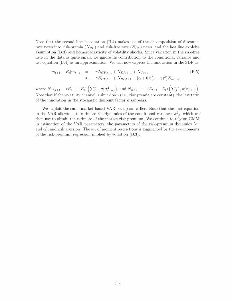
Note that the second line in equation (B.4) makes use of the decomposition of discount-rate news into risk-premia (NRP ) and risk-free rate (NRF ) news, and the last line exploitsassumption (B.3) and homoscedasticity of volatility shocks. Since variation in the risk-freerate in the data is quite small, we ignore its contribution to the conditional variance anduse equation (B.4) as an approximation. We can now express the innovation in the SDF as:

mt+1 − Et[mt+1] = −γNCF,t+1 +NDR,t+1 +NV,t+1 (B.5)

≈ −γNCF,t+1 +NRF,t+1 +(α+ 0.5(1 − γ)2

)Nσ2,t+1 ,

where Nσ2,t+1 ≡ (Et+1 −Et)(∑

∞

j=1 κj1σ

2r,t+j

), and NRF,t+1 ≡ (Et+1 −Et)

(∑∞

j=1 κj1rf,t+j

).

Note that if the volatility channel is shut down (i.e., risk premia are constant), the last termof the innovation in the stochastic discount factor disappears.

We exploit the same market-based VAR set-up as earlier. Note that the first equationin the VAR allows us to estimate the dynamics of the conditional variance, σ2

r,t, which wethen use to obtain the estimate of the market risk premium. We continue to rely on GMMin estimation of the VAR parameters, the parameters of the risk-premium dynamics (α0

and α), and risk aversion. The set of moment restrictions is augmented by the two momentsof the risk-premium regression implied by equation (B.3).

35

References

Bansal, R., R. Dittmar, and C. Lundblad, (2005a), Consumption, dividends, and thecross-section of equity returns, Journal of Finance 60, 1639–1672.

Bansal, R., R. F. Dittmar, and D. Kiku, (2009a), Cointegration and consumptionrisks in asset returns, Review of Financial Studies 22, 1343–1375.

Bansal, R., V. Khatchatrian, and A. Yaron, (2005b), Interpretable asset markets,European Economic Review 49, 531–560.

Bansal, R., D. Kiku, and A. Yaron, (2007a), A note on the economics and statisticsof predictability: A long run risks perspective, Working paper.

Bansal, R., D. Kiku, and A. Yaron, (2007b), Risks for the long run: Estimation andinference, Working paper.

Bansal, R., D. Kiku, and A. Yaron, (2009b), An empirical evaluation of the long-runrisks model for asset prices, Working paper.

Bansal, R. and I. Shaliastovich, (2010), Confidence risks and asset prices, American

Economic Review, papers and proceedings 100, 537–41.

Bansal, R. and A. Yaron, (2004), Risks for the long run: A potential resolution ofasset pricing puzzles, Journal of Finance 59, 1481–1509.

Bollerslev, T. and H. O. Mikkelsen, (1996), Modeling and pricing long memory instock market volatility, Journal of Econometrics 73.

Bollerslev, T., G. Tauchen, and H. Zhou, (2009), Expected stock returns and variancerisk premia, Review of Financial Studies 22.

Breeden, D. T., (1979), An intertemporal asset pricing model with stochastic con-sumption and investment opportunities, Journal of Financial Economics 7, 265–296.

Campbell, J., (1983), Intertemporal asset pricing without consumption data., Amer-

ican Economic Review 83, 487–512.

Campbell, J., (1996), Understanding risk and return, Journal of Political Economy

104, 298–345.

Campbell, J., S. Giglio, C. Polk, and R. Turley, (2011), An intertemporal capm withstochastic volatility, Working paper, Harvard University.

Campbell, J. and T. Vuolteenaho, (2004), Bad beta, good beta, American Economic

Review 94, 1249–1275.

36

Coval, J. D. and T. Shumway, (2001), Expected option returns, Journal of Finance

56(3).

Drechsler, I. and A. Yaron, (2011), What’s vol got to do with it, Review of Financial

Studies 24, 1–45.

Epstein, L. G. and S. Zin, (1989), Substitution, risk aversion and the temporal be-havior of consumption and asset returns: A theoretical framework, Econometrica

57, 937–969.

Epstein, L. G. and S. Zin, (1991), Substitution, risk aversion and the temporal behav-ior of consumption and asset returns: An empirical analysis, Journal of Political

Economy 99, 263–286.

Eraker, B. and I. Shaliastovich, (2008), An equilibrium guide to designing affinepricing models, Mathematical Finance 18, 519–543.

Hansen, L. P., J. C. Heaton, and N. Li, (2008), Consumption strikes back? Measuringlong-run risk, Journal of Political Economy, forthcoming.

Jagannathan, R. and Z. Wang, (1996), The conditional capm and the cross-sectionof expected returns, Journal of Finance 51, 3–53.

Kreps, D. M. and E. L. Porteus, (1978), Temporal resolution of uncertainty anddynamic choice theory, Econometrica 46, 185–200.

Lettau, M. and S. Ludvigson, (2001), Consumption, aggregate wealth, and expectedstock returns, Journal of Finance 56(3).

Lustig, H. and S. Van Nieuwerburgh, (2008), The returns on human capital: Goodnews on wall street is bad news on main street, Review of Financial Studies 21,2097–2137.

McConnell, M. and G. Perez-Quiros, (2000), Output fluctuations in the united states:What has changed since the early 1980s?, American Economic Review 90, 1464–76.

Merton, R. C., (1973), An intertemporal capital asset pricing model, Econometrica

41, 867–887.

Stock, J. and M. Watson, (2002), Has the business cycle change and why?, in Gertler,M. and K. Rogoff, eds., NBER Macroeconomics Annual: 2002 , Cambridge, MA:MIT Press.

Weil, P., (1989), The equity premium puzzle and the risk free rate puzzle, Journal of

Monetary Economics 24, 401–421.

37

Tables and Figures

Table 1: Data Summary Statistics

Mean Std. Dev. AR(1)

Consumption growth 1.86 2.18 0.48Labor income growth 2.01 3.91 0.39Market return 5.70 19.64 -0.01Price-dividend ratio 3.38 0.45 0.88Realized variance 4.76 11.13 0.44

Summary statistics for real consumption growth, real labor income growth, real market return,stock market price-dividend ratio and the realized variance. Realized variance is based on the sumof squared monthly industrial production growth rates over the year, and is re-scaled to match theunconditional variance of consumption growth. Annual observations from 1930 to 2010. Consump-tion growth, labor income growth and market return statistics are in percent; realized variance ismultiplied by 10000.

38

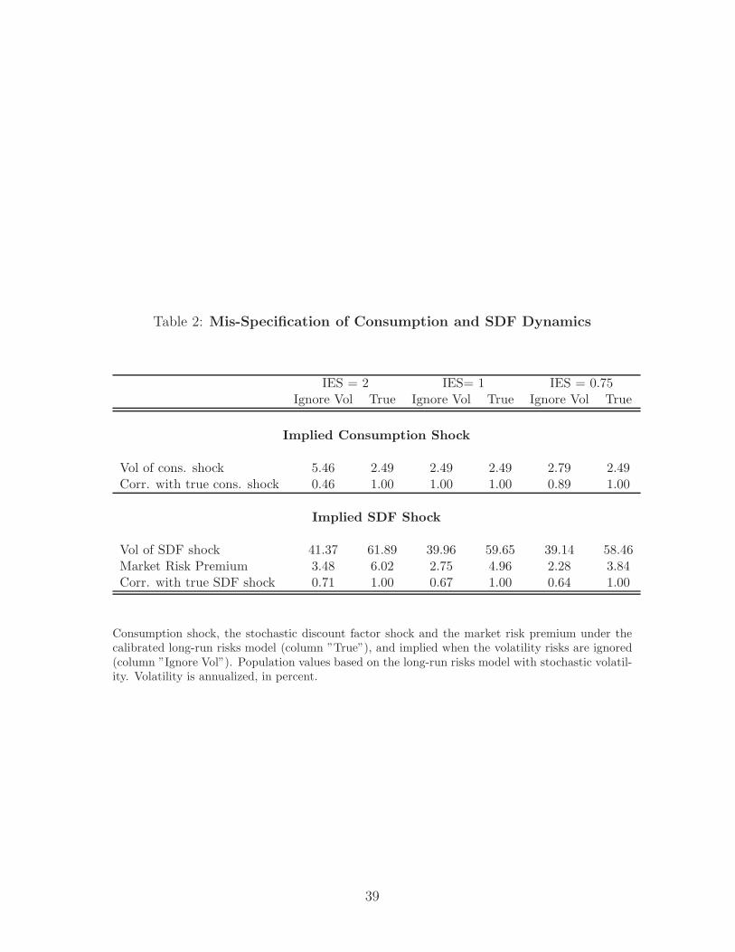
Table 2: Mis-Specification of Consumption and SDF Dynamics

IES = 2 IES= 1 IES = 0.75Ignore Vol True Ignore Vol True Ignore Vol True

Implied Consumption Shock

Vol of cons. shock 5.46 2.49 2.49 2.49 2.79 2.49Corr. with true cons. shock 0.46 1.00 1.00 1.00 0.89 1.00

Implied SDF Shock

Vol of SDF shock 41.37 61.89 39.96 59.65 39.14 58.46Market Risk Premium 3.48 6.02 2.75 4.96 2.28 3.84Corr. with true SDF shock 0.71 1.00 0.67 1.00 0.64 1.00

Consumption shock, the stochastic discount factor shock and the market risk premium under thecalibrated long-run risks model (column ”True”), and implied when the volatility risks are ignored(column ”Ignore Vol”). Population values based on the long-run risks model with stochastic volatil-ity. Volatility is annualized, in percent.

39

Table 3: Macro VAR Estimates

∆ct ∆yt rdt pdt RVt R2

∆ct+1 0.221 0.149 0.058 0.002 2.628 0.61[0.090] [0.037] [0.012] [0.003] [1.091]

∆yt+1 -0.271 0.507 0.079 0.005 2.991 0.36[0.271] [0.146] [0.026] [0.007] [3.417]

rd,t+1 -3.081 1.109 0.065 -0.073 -10.653 0.08[0.881] [0.369] [0.085] [0.037] [10.265]

pdt+1 -3.586 0.974 -0.234 0.921 -8.872 0.80[0.939] [0.647] [0.147] [0.041] [10.856]

RVt+1 -0.007 -0.006 0.001 -0.001 0.310 0.35[0.005] [0.004] [0.0004] [0.0003] [0.091]

Parameter estimates of the Macro VAR which includes real consumption growth ∆c, real labor

income growth ∆y, real market return rd, market price-dividend ratio pd and the realized variance

RV. Realized variance is based on the sum of squared monthly industrial production growth rates

over the year, and is re-scaled to match the unconditional variance of consumption growth. Annual

observations from 1930 to 2010. Robust standard errors are in the brackets.

40

Table 4: Role of Volatility for Economic News

With Vol Risk No Vol RiskNECF NV Nd

DR NyDR NDR NM N

yDR NDR NM

Std. Dev. 5.19 29.72 14.22 2.58 3.91 47.27 4.65 2.60 26.41Corr. with NV -0.27 1.00 0.86 0.28 0.77 0.84 -0.85 -0.27 0.24

Volatility News Periods:Lowest 25% 2.23 -32.57 -12.37 -0.61 -2.96 -44.77 4.48 1.11 -8.13Highest 25% -1.70 36.94 16.02 0.68 3.75 49.90 -5.09 -0.86 8.35

Standard deviation of economic news, correlation with volatility news and the magnitude of the news

in lowest 25% and highest 25% volatility periods. Economic news include news in expected future

consumption NECF , future volatility NV , stochastic discount factor NM , and discount rates on the

market NdDR, labor Ny

DR and wealth return NDR. ”With Vol Risk” columns show the economic news

when the volatility risks are present in the construction of the aggregate wealth portfolio, while ”No

Vol Risk” columns document the implications when volatility risks are ignored. Risk aversion is set

at γ = 5, and IES ψ = 2.

41

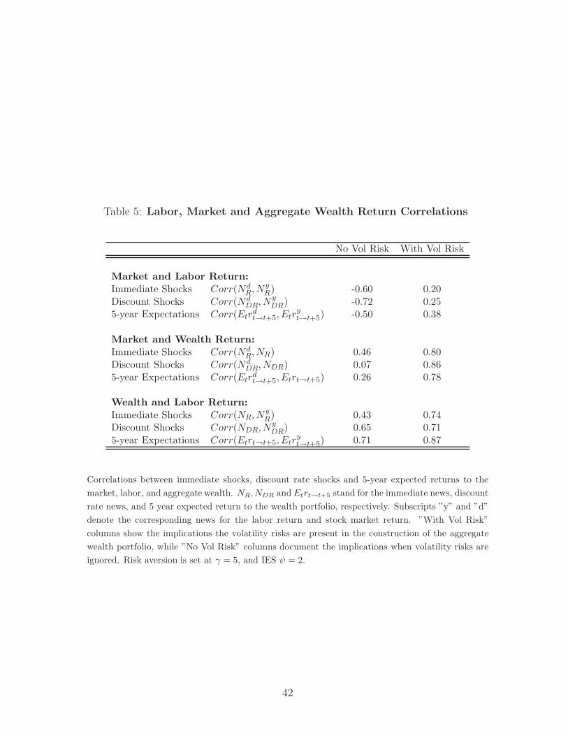
Table 5: Labor, Market and Aggregate Wealth Return Correlations

No Vol Risk With Vol Risk

Market and Labor Return:

Immediate Shocks Corr(NdR, N

yR) -0.60 0.20

Discount Shocks Corr(NdDR, N

yDR) -0.72 0.25

5-year Expectations Corr(Etrdt→t+5, Etr

yt→t+5) -0.50 0.38

Market and Wealth Return:

Immediate Shocks Corr(NdR, NR) 0.46 0.80

Discount Shocks Corr(NdDR, NDR) 0.07 0.86

5-year Expectations Corr(Etrdt→t+5, Etrt→t+5) 0.26 0.78

Wealth and Labor Return:

Immediate Shocks Corr(NR, NyR) 0.43 0.74

Discount Shocks Corr(NDR, NyDR) 0.65 0.71

5-year Expectations Corr(Etrt→t+5, Etryt→t+5) 0.71 0.87

Correlations between immediate shocks, discount rate shocks and 5-year expected returns to the

market, labor, and aggregate wealth. NR, NDR and Etrt→t+5 stand for the immediate news, discount

rate news, and 5 year expected return to the wealth portfolio, respectively. Subscripts ”y” and ”d”

denote the corresponding news for the labor return and stock market return. ”With Vol Risk”

columns show the implications the volatility risks are present in the construction of the aggregate

wealth portfolio, while ”No Vol Risk” columns document the implications when volatility risks are

ignored. Risk aversion is set at γ = 5, and IES ψ = 2.

42

Table 6: Labor, Market and Aggregate Wealth Return Risk Premium

No Vol Risk With Vol Risk

Market Return:

Risk Premium Cov(−NM , NdR) 2.34 7.16

Cash-Flow Risk Premium Cov(−γNCF , NdR) 2.57 2.57

Vol Risk Premium Cov(−NV , NdR) 0 4.28

Discount Rate Risk Premium Cov(−NDR, NdR) -0.23 0.30

Wealth Return:

Risk Premium Cov(−NM , NR) 0.86 2.57Cash-Flow Risk Premium Cov(−γNCF , NR) 0.94 1.20Vol Risk Premium Cov(−NV , NR) 0 1.31Discount Rate Risk Premium Cov(−NDR, NR) -0.08 0.06

Labor Return:

Risk Premium Cov(−NM , NyR) 0.53 1.42

Cash-Flow Risk Premium Cov(−γNCF , NyR) 1.27 0.86

Vol Risk Premium Cov(−NV , NyR) 0 0.57

Discount Rate Risk Premium Cov(−NDR, NyR) -0.04 0.00

Total risk premium on labor, market and wealth return, and its decomposition into cash-flow,

discount rate and volatility risk premium components. NM denotes the stochastic discount factor

shock, and NCF , NDR and NV represent the current and future cash-flow news, discount rate news

on the wealth portfolio and volatility news. NR, NyR and Nm

R denote the immediate return news to

wealth, labor and market, respectively. ”With Vol Risk” columns show the implications the volatility

risks are present in the construction of the aggregate wealth portfolio, while ”No Vol Risk” columns

document the implications when volatility risks are ignored. Risk aversion is set at γ = 5, and IES

ψ = 2.

43

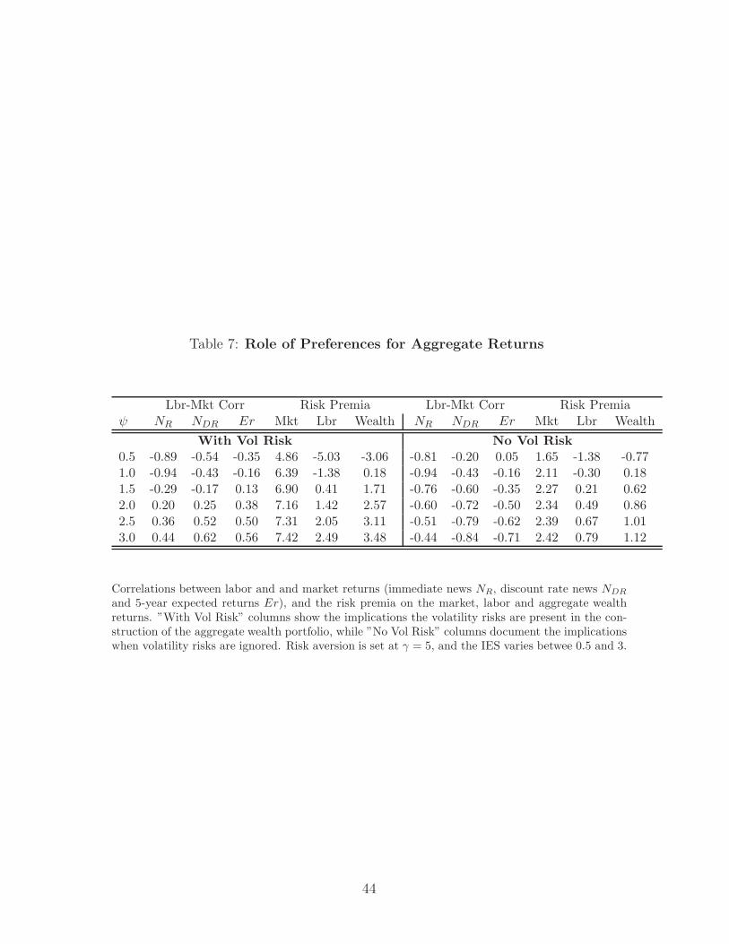
Table 7: Role of Preferences for Aggregate Returns

Lbr-Mkt Corr Risk Premia Lbr-Mkt Corr Risk Premiaψ NR NDR Er Mkt Lbr Wealth NR NDR Er Mkt Lbr Wealth

With Vol Risk No Vol Risk

0.5 -0.89 -0.54 -0.35 4.86 -5.03 -3.06 -0.81 -0.20 0.05 1.65 -1.38 -0.771.0 -0.94 -0.43 -0.16 6.39 -1.38 0.18 -0.94 -0.43 -0.16 2.11 -0.30 0.181.5 -0.29 -0.17 0.13 6.90 0.41 1.71 -0.76 -0.60 -0.35 2.27 0.21 0.622.0 0.20 0.25 0.38 7.16 1.42 2.57 -0.60 -0.72 -0.50 2.34 0.49 0.862.5 0.36 0.52 0.50 7.31 2.05 3.11 -0.51 -0.79 -0.62 2.39 0.67 1.013.0 0.44 0.62 0.56 7.42 2.49 3.48 -0.44 -0.84 -0.71 2.42 0.79 1.12

Correlations between labor and and market returns (immediate news NR, discount rate news NDR

and 5-year expected returns Er), and the risk premia on the market, labor and aggregate wealthreturns. ”With Vol Risk” columns show the implications the volatility risks are present in the con-struction of the aggregate wealth portfolio, while ”No Vol Risk” columns document the implicationswhen volatility risks are ignored. Risk aversion is set at γ = 5, and the IES varies betwee 0.5 and 3.

44

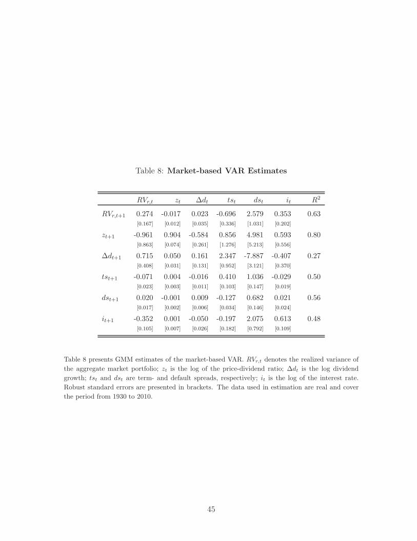
Table 8: Market-based VAR Estimates

RVr,t zt ∆dt tst dst it R2

RVr,t+1 0.274 -0.017 0.023 -0.696 2.579 0.353 0.63[0.167] [0.012] [0.035] [0.336] [1.031] [0.202]

zt+1 -0.961 0.904 -0.584 0.856 4.981 0.593 0.80[0.863] [0.074] [0.261] [1.276] [5.213] [0.556]

∆dt+1 0.715 0.050 0.161 2.347 -7.887 -0.407 0.27[0.408] [0.031] [0.131] [0.952] [3.121] [0.370]

tst+1 -0.071 0.004 -0.016 0.410 1.036 -0.029 0.50[0.023] [0.003] [0.011] [0.103] [0.147] [0.019]

dst+1 0.020 -0.001 0.009 -0.127 0.682 0.021 0.56[0.017] [0.002] [0.006] [0.034] [0.146] [0.024]

it+1 -0.352 0.001 -0.050 -0.197 2.075 0.613 0.48[0.105] [0.007] [0.026] [0.182] [0.792] [0.109]

Table 8 presents GMM estimates of the market-based VAR. RVr,t denotes the realized variance of

the aggregate market portfolio; zt is the log of the price-dividend ratio; ∆dt is the log dividend

growth; tst and dst are term- and default spreads, respectively; it is the log of the interest rate.

Robust standard errors are presented in brackets. The data used in estimation are real and cover

the period from 1930 to 2010.

45

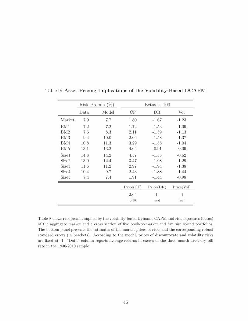
Table 9: Asset Pricing Implications of the Volatility-Based DCAPM

Risk Premia (%) Betas × 100

Data Model CF DR Vol

Market 7.9 7.7 1.80 -1.67 -1.23

BM1 7.2 7.2 1.72 -1.53 -1.09BM2 7.6 8.3 2.11 -1.59 -1.13BM3 9.4 10.0 2.66 -1.58 -1.37BM4 10.8 11.3 3.29 -1.58 -1.04BM5 13.1 13.2 4.64 -0.91 -0.09

Size1 14.8 14.2 4.57 -1.55 -0.62Size2 13.0 12.4 3.47 -1.98 -1.29Size3 11.6 11.2 2.97 -1.94 -1.38Size4 10.4 9.7 2.43 -1.88 -1.44Size5 7.4 7.4 1.91 -1.44 -0.98

Price(CF) Price(DR) Price(Vol)

2.64 -1 -1[0.38] [na] [na]

Table 9 shows risk premia implied by the volatility-based Dynamic CAPM and risk exposures (betas)

of the aggregate market and a cross section of five book-to-market and five size sorted portfolios.

The bottom panel presents the estimates of the market prices of risks and the corresponding robust

standard errors (in brackets). According to the model, prices of discount-rate and volatility risks

are fixed at -1. “Data” column reports average returns in excess of the three-month Treasury bill

rate in the 1930-2010 sample.

46

Table 10: Asset Pricing Implications of the Restricted Volatility-Based

DCAPM

Risk Premia (%) Betas × 100

Data Model CF RF Vol

Market 7.9 7.6 1.98 -0.02 -1.93

BM1 7.2 7.0 1.92 0.19 -1.76BM2 7.6 8.3 2.30 0.10 -1.81BM3 9.4 10.2 2.80 -0.09 -2.09BM4 10.8 11.4 3.39 -0.17 -1.58BM5 13.1 13.0 4.54 -0.04 -0.05

Size1 14.8 14.1 4.63 0.07 -0.96Size2 13.0 12.5 3.67 0.07 -2.06Size3 11.6 11.3 3.19 0.05 -2.20Size4 10.4 9.8 2.63 -0.05 -2.25Size5 7.4 7.4 2.04 -0.04 -1.52

Price(CF) Price(RF) Price(Vol)

2.85 -1 -1[0.45] [na] [na]

Table 10 shows risk premia implied by the restricted volatility-based Dynamic CAPM and risk

exposures (betas) of the aggregate market and a cross section of five book-to-market and five size

sorted portfolios. In this specification, discount-rate variation is decomposed into variation in risk

premia (which are proportional to the conditional market variance) and variation in the risk-free

rate. The bottom panel presents the estimates of the market prices of risks and the corresponding

robust standard errors (in brackets). According to the model, prices of risk-free and volatility news

are fixed at -1. “Data” column reports average returns in excess of the three-month Treasury bill

rate in the 1930-2010 sample.

47

Figure 1: Volatility and Expected Consumption Growth from Macro VAR

1930 1940 1950 1960 1970 1980 1990 2000 2010−3

−2

−1

0

1

2

3

4

5

Cons. VolExp. Cons.

Ex-ante consumption volatility (solid line) and expected consumption growth (dashed line) implied

from Macro VAR. The two series are standardized. Shaded areas represent the NBER recession

dates.

Figure 2: Consumption Response to Volatility Shock from Macro VAR

0 1 2 3 4−0.8

−0.7

−0.6

−0.5

−0.4

−0.3

−0.2

−0.1

0

Impulse response of consumption growth to one standard deviation shock in ex-ante volatility of

consumption, implied by the Macro VAR. One standard deviation volatility shock corresponds to an

increase in ex-ante consumption variance by (1.95%)2. Consumption growth is annual, in per cent.

48

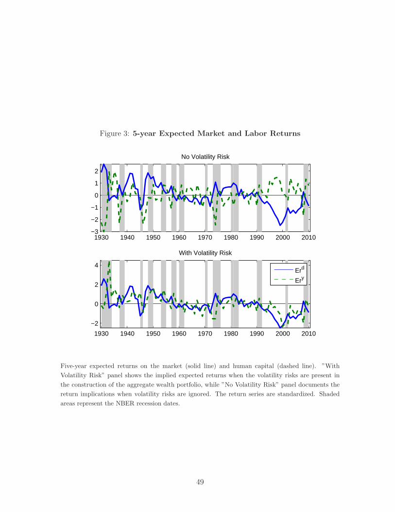
Figure 3: 5-year Expected Market and Labor Returns

1930 1940 1950 1960 1970 1980 1990 2000 2010−3

−2

−1

0

1

2

No Volatility Risk

1930 1940 1950 1960 1970 1980 1990 2000 2010

−2

0

2

4

With Volatility Risk

Erd

Ery

Five-year expected returns on the market (solid line) and human capital (dashed line). ”With

Volatility Risk” panel shows the implied expected returns when the volatility risks are present in

the construction of the aggregate wealth portfolio, while ”No Volatility Risk” panel documents the

return implications when volatility risks are ignored. The return series are standardized. Shaded

areas represent the NBER recession dates.

49

Figure 4: Discount Rate and Volatility News

1940 1950 1960 1970 1980 1990 2000 2010

−3

−2

−1

0

1

2

3

N

DR

NV

Discount rate news on the wealth portfolio NDR and the volatility news NV . The news series are

standardized. Shaded areas represent the NBER recession dates.

50

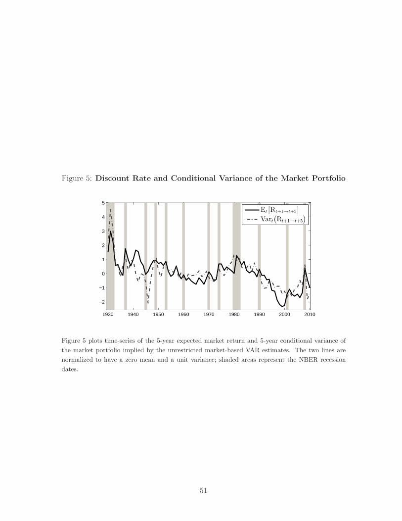
Figure 5: Discount Rate and Conditional Variance of the Market Portfolio

1930 1940 1950 1960 1970 1980 1990 2000 2010

−2

−1

0

1

2

3

4

5

Et

[

Rt+1→t+5

]

Vart

(

Rt+1→t+5

)

Figure 5 plots time-series of the 5-year expected market return and 5-year conditional variance of

the market portfolio implied by the unrestricted market-based VAR estimates. The two lines are

normalized to have a zero mean and a unit variance; shaded areas represent the NBER recession

dates.

51

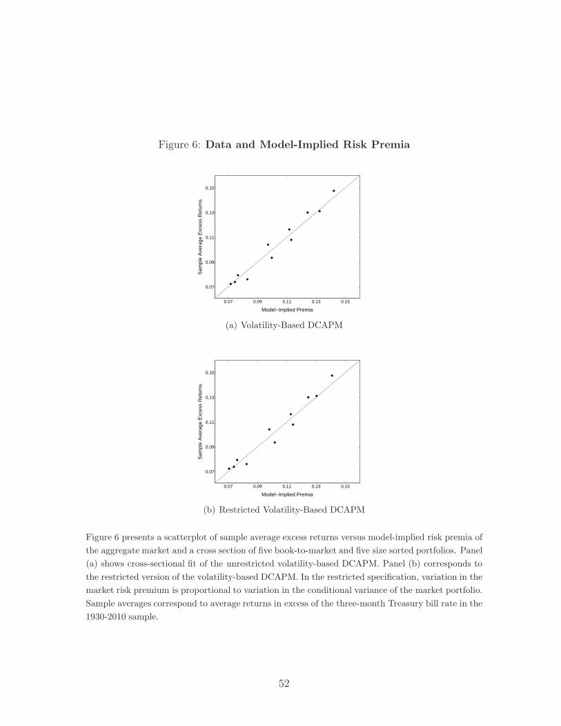
Figure 6: Data and Model-Implied Risk Premia

0.07 0.09 0.11 0.13 0.15

0.07

0.09

0.11

0.13

0.15

Model−Implied Premia

Sam

ple

Ave

rage

Exc

ess

Ret

urns

(a) Volatility-Based DCAPM

0.07 0.09 0.11 0.13 0.15

0.07

0.09

0.11

0.13

0.15

Model−Implied Premia

Sam

ple

Ave

rage

Exc

ess

Ret

urns

(b) Restricted Volatility-Based DCAPM

Figure 6 presents a scatterplot of sample average excess returns versus model-implied risk premia of

the aggregate market and a cross section of five book-to-market and five size sorted portfolios. Panel

(a) shows cross-sectional fit of the unrestricted volatility-based DCAPM. Panel (b) corresponds to

the restricted version of the volatility-based DCAPM. In the restricted specification, variation in the

market risk premium is proportional to variation in the conditional variance of the market portfolio.

Sample averages correspond to average returns in excess of the three-month Treasury bill rate in the

1930-2010 sample.

52