Volatility estimation for stochastic PDEs using high-frequencyobservations

Markus Bibingera, Mathias Trabs∗b

aFachbereich 12 Mathematik und Informatik, Philipps-Universitat Marburg, bibinger@uni-marburg.debFachbereich Mathematik, Universitat Hamburg, mathias.trabs@uni-hamburg.de

AbstractWe study the parameter estimation for parabolic, linear, second-order, stochastic partial differential equa-tions (SPDEs) observing a mild solution on a discrete grid in time and space. A high-frequency regime isconsidered where the mesh of the grid in the time variable goes to zero. Focusing on volatility estimation,we provide an explicit and easy to implement method of moments estimator based on squared increments.The estimator is consistent and admits a central limit theorem. This is established moreover for the jointestimation of the integrated volatility and parameters in the differential operator in a semi-parametric frame-work. Starting from a representation of the solution of the SPDE with Dirichlet boundary conditions asan infinite factor model and exploiting mixing-type properties of time series, the theory considerably dif-fers from the statistics for semi-martingales literature. The performance of the method is illustrated in asimulation study.

Keywords: high-frequency data, stochastic partial differential equation, random field, realized volatility,mixing-type limit theorem

2010 MSC: 62M10, 60H15

1. Introduction

1.1. OverviewMotivated by random phenomena in natural science as well as by mathematical finance, stochastic

partial differential equations (SPDEs) have been intensively studied during the last fifty years with a mainfocus on theoretical analytic and probabilistic aspects. Thanks to the exploding number of available dataand the fast progress in information technology, SPDE models become nowadays increasingly popular forpractitioners, for instance, to model neuronal systems or interest rate fluctuations. Consequently, statisticalmethods are required to calibrate this class of complex models. While in probability theory there arerecently enormous efforts to advance research for SPDEs, for instance Hairer (2013) was able to solve theKPZ equation, there is scant groundwork on statistical inference for SPDEs and there remain many openquestions.

Considering discrete high-frequency data in time, our aim is to extend the well understood statisticaltheory for semi-martingales, see, for instance, Jacod and Protter (2012) and Mykland and Zhang (2009), toparabolic SPDEs which can be understood as infinite dimensional stochastic differential equations. Gen-erated by an infinite factor model, high-frequency dynamics of the SPDE model differ from the semi-martingale case in several ways. The SPDE model induces a distinctive, much rougher behavior of themarginal processes over time for a fixed spatial point compared to semi-martingales or diffusion processes.In particular, they have infinite quadratic variation and a nontrivial quartic variation, cf. Swanson (2007).Also, we find non-negligible negative autocovariances of increments such that the semi-martingale theoryand martingale central limit theorems are not applicable to the marginal processes. Nevertheless, we showthat the fundamental concept of realized volatility as a key statistic can be adapted to the SPDE setting.While this work provides a foundation and establishes first results, we are convinced that more conceptsfrom the high-frequency semi-martingale literature can be fruitfully transferred to SPDE models.

∗Corresponding author.

1

arX

iv:1

710.

0351

9v3

[m

ath.

ST]

10

Sep

2019

We consider the following linear parabolic SPDE with one space dimension

dXt(y) =(ϑ2∂2Xt(y)

∂y2+ ϑ1

∂Xt(y)

∂y+ ϑ0Xt(y)

)dt+ σt dBt(y), X0(y) = ξ(y) (1)

(t, y) ∈ R+ × [ymin, ymax], Xt(ymin) = Xt(ymax) = 0 for t > 0,

where Bt is defined as a cylindrical Brownian motion in a Sobolev space on [ymin, ymax], the initial valueξ is independent fromB, and with parameters ϑ0, ϑ1 ∈ R and ϑ2 > 0 and some volatility function σ whichwe assume to depend only on time. The simple Dirichlet boundary conditions Xt(ymin) = Xt(ymax) = 0are natural in many applications. We also briefly touch on enhancements to other boundary conditions.

A solution X = {Xt(y), (t, y) ∈ [0, T ] × [ymin, ymax]} of (1) will be observed on a discrete grid(ti, yj) ⊆ [0, T ]× [ymin, ymax] for i = 1, . . . , n and j = 1, . . . ,m in a fixed rectangle. More specificallywe consider equidistant time points ti = i∆n. While the parameter vector ϑ = (ϑ0, ϑ1, ϑ2)> mightbe known from the physical foundation of the model, estimating σ2 quantifies the level of variability orrandomness in the system. This constitutes our first target of inference. An extension of our approach forinference on ϑ will also be discussed.

1.2. Literature

The key insight in the pioneering work by Hubner et al. (1993) is that for a large class of parabolicdifferential equations the solution of the SPDE can be written as a Fourier series where each Fourier coef-ficient follows an ordinary stochastic differential equation of Ornstein-Uhlenbeck type. Hence, statisticalprocedures for these latter processes offer a possible starting point for inference on the SPDE. Most ofthe available literature on statistics for SPDEs studies a scenario with observations of the Fourier coef-ficients in the spectral representation of the equation, see for instance Hubner and Rozovskiı (1995) andCialenco and Glatt-Holtz (2011) for the maximum likelihood estimation for linear and non-linear SPDEs,respectively. Bishwal (2002) discusses a Bayesian approach and Cialenco et al. (2018) a trajectory fittingprocedure. Hubner and Lototsky (2000) and Prakasa Rao (2002) have studied nonparametric estimatorswhen the Fourier coefficients are observed continuously or in discrete time, respectively. We refer to thesurveys by Lototsky (2009) and Cialenco (2018) for an overview on the existing theory.

The (for many applications) more realistic scenario where the solution of a SPDE is observed only atdiscrete points in time and space has been considered so far only in very few works. Markussen (2003) hasderived asymptotic normality and efficiency for the maximum likelihood estimator in a parametric problemfor a parabolic SPDE. Mohapl (1997) has considered maximum likelihood and least squares estimators fordiscrete observations of an elliptic SPDE where the dependence structure of the observations is howevercompletely different (in fact simpler) from the parabolic case.

Our theoretical setup differs from the one in Markussen (2003) in several ways. First, we introduce atime varying volatility σt in the disturbance term. Second, we believe that discrete high-frequency data intime under infill asymptotics, where we have a finite time horizon [0, T ] and in the asymptotic theory themesh of the grid tends to zero, are most informative for many prospective data applications. Markussen(2003) instead focused on a low-frequency setup where the number of observations in time tends to infinityat a fixed time step. Also his number of observations in space is fixed, but we allow for an increasingnumber of spatial observations, too.

There are two very recent related works by Cialenco and Huang (2019) and Chong (2018). In theseindependent projects the authors establish results for power variations in similar models, when ϑ1 = 0.Cialenco and Huang (2019) prove central limit theorems in a parametric model when either m = 1 andn → ∞, or n = 1 and m → ∞. For an unbounded spatial domain, Chong (2018) establishes a limittheorem for integrated volatility estimation when m is fixed and n → ∞. While some of our results arerelated, we provide the first limit theorem under double asymptotics when n → ∞ and m → ∞, and forthe joint estimation of the volatility and an unknown parameter in the differential operator. Interestingly,the proofs of the three works are based on very different technical ingredients – while we use mixing theoryfor time series the results by Cialenco and Huang (2019) rely on tools from Malliavin calculus and Chong(2018) conducts a martingale approximation by truncation and blocking techniques to apply results byJacod (1997).

2

1.3. MethodologyThe literature on statistics for high-frequency observations of semi-martingales suggests to use the sum

of squared increments in order to estimate the volatility. While in the present infinite dimensional modelthis remains generally possible, there are some deep structural differences. Supposing that σt is at least1/2-Holder regular, we show for any fixed spatial point y ∈ (ymin, ymax) the convergence in probability

RVn(y) :=1

n√

∆n

n∑i=1

(∆iX)2(y)P→ e−y ϑ1/ϑ2

√ϑ2π

∫ T

0

σ2t dt for n→∞,

where ∆iX(y) := Xi∆n(y) − X(i−1)∆n

(y),∆n = T/n. For a semi-martingale instead, squared incre-ments are of order ∆n and not

√∆n. We also see a dependence of the realized volatility on the spatial

position y. Assuming ϑ1, ϑ2 to be known and exploiting this convergence, the construction of a consistentmethod of moments estimator for the integrated volatility is obvious. However, the proof of a central limittheorem for such an estimator is non-standard.

The method of moments can be extended from one to m spatial observations where m is a fixed integeras n → ∞, or in the double asymptotic regime where n → ∞ and m → ∞. It turns out that therealized volatilities (RVn(yj))16j6m even de-correlate asymptotically when m2∆n → 0. We prove thatthe final estimator attains a parametric

√mn-rate and satisfies a central limit theorem. Since we have

negative autocorrelations between increments (∆iX(yj))16i6n, a martingale central limit theorem cannotbe applied. Instead, we apply a central limit theorem for weakly dependent triangular arrays by Peligradand Utev (1997). Introducing a quarticity estimator, we also provide a feasible version of the limit theoremthat allows for the construction of confidence intervals.

In view of the complex probabilistic model, our estimator is strikingly simple. Thanks to its explicitform that does not rely on optimization algorithms, the method can be easily implemented and the compu-tation is very fast. An M-estimation approach can be used to construct a joint estimator of the parameters in(1). While the volatility estimator is first constructed in the simplified parametric framework, by a carefuldecomposition of approximation errors we derive asymptotic results for the semi-parametric estimation ofthe integrated volatility under quite general assumptions.

1.4. ApplicationsAlthough (1) is a relatively simple SPDE model, it already covers many interesting applications. Let

us give some examples:1. The stochastic heat equation

dXt(y) = ϑ2∂2Xt(y)

∂y2dt+ ϑ0Xt(y) dt+ σt dBt(y) ,

with thermal diffusivity ϑ2 > 0, is the prototypical example for parabolic SPDEs. With a dissipationrate ϑ0 6= 0, the SPDE describes the temperature in space and time of a system under cooling orheating.

2. The cable equation is a basic PDE-model in neurobiology, cf. Tuckwell (2013). Modeling the nervemembrane potential, its stochastic version is given by

cm dVt(y) =( 1

ri

∂2Vt(y)

∂y2− Vt(y)

rm

)dt+ σt dBt(y), 0 < y < l, t > 0,

where y is the length from the left endpoint of the cable with total length l > 0 and t is time. Theparameters are the membrane capacity cm > 0, the resistance of the internal medium ri > 0 and themembrane resistance rm > 0. The noise terms represent the synaptic input. The first mathematicaltreatment of this equation goes back to Walsh (1986).

3. The term structure model by Cont (2005). It describes a yield curve as a random field, i.e. a contin-uous function of time t and time to maturity y ∈ [ymin, ymax]. Differently than classical literatureon time-continuous interest rate models in mathematical finance, including the landmark paper byHeath et al. (1992) and ensuing work, which focus on modeling arbitrage-free term structure evolu-tions under risk-neutral measures, Cont (2005) aims to describe real-world dynamics of yield curves.

3

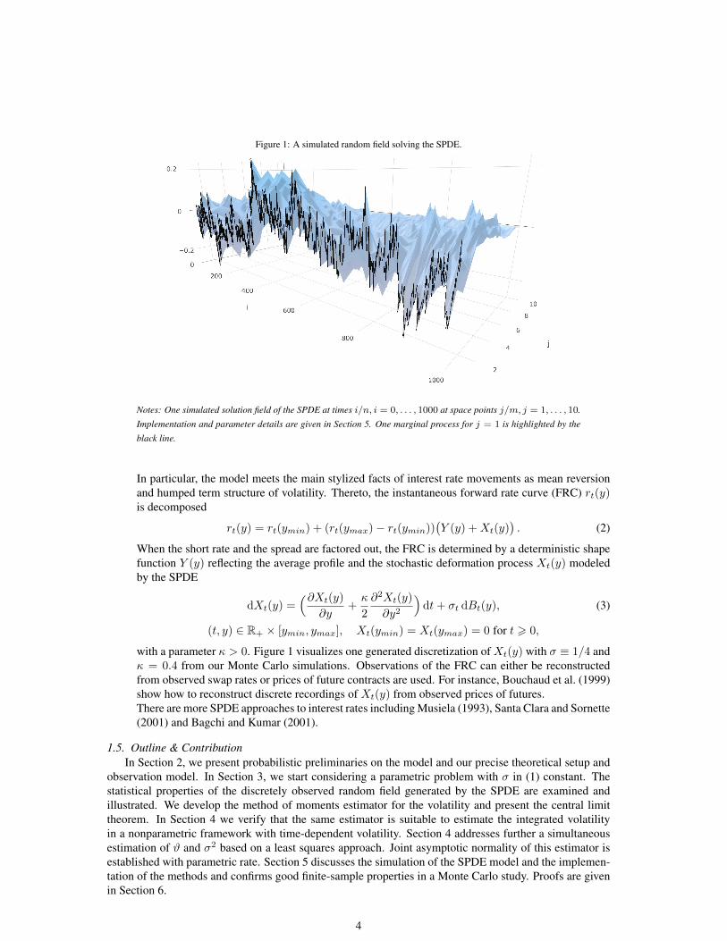
Figure 1: A simulated random field solving the SPDE.

Notes: One simulated solution field of the SPDE at times i/n, i = 0, . . . , 1000 at space points j/m, j = 1, . . . , 10.

Implementation and parameter details are given in Section 5. One marginal process for j = 1 is highlighted by the

black line.

In particular, the model meets the main stylized facts of interest rate movements as mean reversionand humped term structure of volatility. Thereto, the instantaneous forward rate curve (FRC) rt(y)is decomposed

rt(y) = rt(ymin) + (rt(ymax)− rt(ymin))(Y (y) +Xt(y)

). (2)

When the short rate and the spread are factored out, the FRC is determined by a deterministic shapefunction Y (y) reflecting the average profile and the stochastic deformation process Xt(y) modeledby the SPDE

dXt(y) =(∂Xt(y)

∂y+κ

2

∂2Xt(y)

∂y2

)dt+ σt dBt(y), (3)

(t, y) ∈ R+ × [ymin, ymax], Xt(ymin) = Xt(ymax) = 0 for t > 0,

with a parameter κ > 0. Figure 1 visualizes one generated discretization of Xt(y) with σ ≡ 1/4 andκ = 0.4 from our Monte Carlo simulations. Observations of the FRC can either be reconstructedfrom observed swap rates or prices of future contracts are used. For instance, Bouchaud et al. (1999)show how to reconstruct discrete recordings of Xt(y) from observed prices of futures.There are more SPDE approaches to interest rates including Musiela (1993), Santa Clara and Sornette(2001) and Bagchi and Kumar (2001).

1.5. Outline & ContributionIn Section 2, we present probabilistic preliminaries on the model and our precise theoretical setup and

observation model. In Section 3, we start considering a parametric problem with σ in (1) constant. Thestatistical properties of the discretely observed random field generated by the SPDE are examined andillustrated. We develop the method of moments estimator for the volatility and present the central limittheorem. In Section 4 we verify that the same estimator is suitable to estimate the integrated volatilityin a nonparametric framework with time-dependent volatility. Section 4 addresses further a simultaneousestimation of ϑ and σ2 based on a least squares approach. Joint asymptotic normality of this estimator isestablished with parametric rate. Section 5 discusses the simulation of the SPDE model and the implemen-tation of the methods and confirms good finite-sample properties in a Monte Carlo study. Proofs are givenin Section 6.

4

2. Probabilistic structure and statistical model

Without loss of generality, we set ymin = 0 and ymax = 1. We apply the semi-group approach byDa Prato and Zabczyk (1992) to analyze the SPDE (1) which is associated to the differential operator

Aϑ := ϑ0 + ϑ1∂

∂y+ ϑ2

∂2

∂y2

such that the SPDE (1) reads as dXt(y) = AϑXt(y) dt + σt dBt(y). The eigenfunctions ek of Aϑ withcorresponding eigenvalues −λk are given by

ek(y) =√

2 sin(πky

)exp

(− ϑ1

2ϑ2y), y ∈ [0, 1], (4)

λk = −ϑ0 +ϑ2

1

4ϑ2+ π2k2ϑ2, k ∈ N. (5)

This eigendecomposition takes a key role in our analysis and for the probabilistic properties of the model.Of particular importance is that λk increase proportionally with k2, λk ∝ k2, and that ek(y) dependexponentially on y with an additional oscillating factor. Note that (ek)k>1 is an orthonormal basis of theHilbert space Hϑ := {f : [0, 1]→ R : ‖f‖ϑ <∞} with

〈f, g〉ϑ :=

∫ 1

0

eyϑ1/ϑ2f(y)g(y) dy and ‖f‖2ϑ := 〈f, f〉ϑ.

We choose Hϑ as state space for the solutions of (1). In particular, we suppose that ξ ∈ Hϑ. Aϑ is self-adjoint on Hϑ and the domain of Aϑ is {f ∈ Hϑ : ‖f ′‖ϑ, ‖f ′′‖ϑ <∞, f(0) = f(1) = 0}. The cylindricalBrownian motion (Bt)t>0 in (1) can be defined via

〈Bt, f〉ϑ =∑k>1

〈f, ek〉ϑW kt , f ∈ Hϑ, t > 0,

for independent real-valued Brownian motions (W kt )t>0, k > 1. Xt(y) is called a mild solution of (1) on

[0, T ] if it satisfies the integral equation for any t ∈ [0, T ]

Xt = etAϑξ +

∫ t

0

e(t−s)Aϑσs dBs a.s.

Defining the coordinate processes xk(t) := 〈Xt, ek〉ϑ, t > 0, for any k > 1, the random field Xt(y) canthus be represented as the infinite factor model

Xt(y) =∑k>1

xk(t)ek(y) with xk(t) = e−λkt〈ξ, ek〉ϑ +

∫ t

0

e−λk(t−s)σs dW ks . (6)

In other words, the coordinates xk satisfy the Ornstein-Uhlenbeck dynamics

dxk(t) = −λkxk(t)dt+ σt dW kt , xk(0) = 〈ξ, ek〉ϑ . (7)

There is a modification of the stochastic convolution∫ ·

0e(·−s)Aϑσs dBs which is continuous in time and

space and thus we may assume that (t, y) 7→ Xt(y) is continuous, cf. Da Prato and Zabczyk (1992, Thm.5.22). The neat representation (6) separates dependence on time and space and connects the SPDE modelto stochastic processes in Hilbert spaces. This structure has been exploited in several works, especially forfinancial applications, see, for instance, Bagchi and Kumar (2001) and Schmidt (2006). We consider thefollowing observation scheme.

Assumption 2.1 (Observations). Suppose we observe a mild solution X of (1) on a discrete grid (ti, yj) ∈[0, 1]2 with

ti = i∆n for i = 0, . . . , n and δ 6 y1 < y2 < · · · < ym 6 1− δ (8)where n,m ∈ N and δ > 0. We consider an infill asymptotics regime where n∆n = 1, ∆n → 0 as n→∞and m <∞ is either fixed or it may diverge, m→∞, such that m = mn = O(nρ) for some ρ ∈ (0, 1/2).We assume that m ·minj=2,...,m |yj − yj−1| is bounded from below, uniformly in n.

5

Here and throughout, we write An = O(Bn), if there exist a constant C > 0 independent of m,n, andof potential indices 1 6 i 6 n or 1 6 j 6 m, and some n0 ∈ N, such that |An| 6 CBn for all n > n0.While we have fixed the time horizon to T = 1, the subsequent results can be easily extended to any finiteT . We write ∆iX(y) = Xi∆n

(y)−X(i−1)∆n(y), 1 6 i 6 n, for the increments of the marginal processes

in time and analogously for increments of other processes.The condition m = O(nρ) for some ρ ∈ (0, 1/2) implies that we provide asymptotic results for

discretizations which are finer in time than in space. For instance in the case of an application to termstructure data, this appears quite natural, since we can expect many observations over time of a moderatenumber of different maturities. Especially for financial high-frequency intra-day data, we typically haveat hand several thousands intra-day price recordings per day, but usually at most 10 frequently tradeddifferent maturities. For instance, Eurex offers four classes of German government bonds with differentcontract lengths.2 For each, futures with 2-3 different maturities are traded on a high-frequency basis.While we can thus extract observations in at most 12 different spatial points from this data, 5000-10000intra-daily prices are available, see (Winkelmann et al., 2016, Sec. 4). The relation between m = 15 and nis similar in Bouchaud et al. (1999), where, however, daily prices are used.

We impose the following mild regularity conditions on the initial value of the SPDE (1).

Assumption 2.2. In (1) we assume that

(i) either E[〈ξ, ek〉ϑ] = 0 for all k > 1 and supk λkE[〈ξ, ek〉2ϑ] <∞ holds true orE[‖A1/2

ϑ ξ‖2ϑ] <∞;(ii) (〈ξ, ek〉ϑ)k>1 are independent.

This assumption is especially satisfied if ξ is distributed according to the stationary distribution of (1),where 〈ξ, ek〉ϑ are independently N (0, σ2/(2λk))-distributed. Note also that E[‖A1/2

ϑ ξ‖2ϑ] < ∞ impliessupk λkE[〈ξ, ek〉2ϑ] = supk E[〈A1/2

ϑ ξ, ek〉2ϑ] <∞. Assuming independence of the sequence (〈ξ, ek〉ϑ)k>1

is a convenient condition for an analysis of the variance-covariance structure of our estimator, but could bereplaced by other moment-type conditions on the coefficients of the initial value.

Remark 2.3. Due to the first-order term in (1), when ϑ1 6= 0, our solution is in general not symmetricin space. One may expect, however, symmetry in the following sense: For ϑ0 = 0, starting in ξ = 0, thelaw of Xt(1/2 + r), r ∈ [0, 1/2], with ϑ1 > 0 should be the same as the law of Xt(1/2 − r) with theparameter −ϑ1. This property is satisfied, when we illustrate the solution (6) with respect to the modifiedeigenfunctions

ek(y) :=√

2 sin(πky) exp(− ϑ1

2ϑ2

(y − 1

2

))= ek(y)eϑ1/(4ϑ2) ,

corresponding to the same eigenvalues −λk, which form an orthonormal basis of L2([0, 1]) with respectto the scalar product 〈f, g〉 =

∫ 1

0e(y−1/2)ϑ1/ϑ2f(y)g(y)dy. Then ek(1/2 + r) for parameter ϑ1 equals

±ek(1/2− r) for parameter −ϑ1, where the sign depends on k, and the symmetric centered Gaussian dis-tribution of xk(t) ensures the discussed symmetry of the law of Xt(y) around y = 1/2. This adjustment bymultiplying the constant exp(ϑ1/(4ϑ2)), which depends on ϑ but not on y or t, can be easily incorporatedin all our results.

3. Estimation of the volatility parameter

In this section, we consider the parametric problem where σ is a constant volatility parameter. Supposefirst that we want to estimate σ2 based on n → ∞ discrete recordings of Xt(y), along only one spatialobservation y ∈ (δ, 1− δ), δ > 0, m = 1. Let us assume first that ϑ is known. We thus know (λk, ek)k>1

explicitly from (5). In many applications, ϑ will be given in the model or reliable estimates could beavailable from historical data. Nevertheless, we address the parameter estimation of ϑ in Section 4.

Volatility estimation relies typically on squared increments of the observed process. We develop amethod of moment estimator here utilizing squared increments (∆iX)2(y), 1 6 i 6 n, too. However, the

2see www.eurexchange.com/exchange-en/products/int

6

behavior of the latter is quite different compared to the standard setup of high-frequency observations ofsemi-martingales.

Though we do not observe the factor coordinate processes in (6), understanding the dynamics of theirincrements is an important ingredient of the analysis of (∆iX)2(y), 1 6 i 6 n. The increments of theOrnstein-Uhlenbeck processes from (6) can be decomposed as

∆ixk = 〈ξ, ek〉ϑ(e−λki∆n − e−λk(i−1)∆n

)︸ ︷︷ ︸=Ai,k

+

∫ (i−1)∆n

0

σe−λk((i−1)∆n−s)(e−λk∆n − 1) dW ks︸ ︷︷ ︸

=Bi,k

+

∫ i∆n

(i−1)∆n

σe−λk(i∆n−s) dW ks .︸ ︷︷ ︸

=Ci,k

(9)

For a fixed finite intensity parameter λk, observing ∆ixk corresponds to the classical semi-martingaleframework. In this case, Ai,k, Bi,k are asymptotically negligible and the exponential term in Ci,k is closeto one, such that σ2 is estimated via the sum of squared increments. Convergence to the quadratic variationwhen n→∞ implies consistency of this estimator, well-known as the realized volatility.

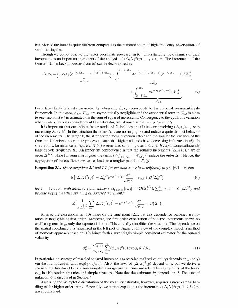
It is important that our infinite factor model of X includes an infinite sum involving (∆ixk)k>1 withincreasing λk ∝ k2. In this situation the terms Bi,k are not negligible and induce a quite distinct behaviorof the increments. The larger k, the stronger the mean reversion effect and the smaller the variance of theOrnstein-Uhlenbeck coordinate processes, such that higher addends have decreasing influence in (6). Insimulations, for instance in Figure 2,Xt(y) is generated summing over 1 6 k 6 K, up to some sufficientlylarge cut-off frequency K. An important consequence is that the squared increments (∆iX(y))2 are oforder ∆

1/2n , while for semi-martingales the terms (W k

(i+1)∆n−W k

i∆n)2 induce the order ∆n. Hence, the

aggregation of the coefficient processes leads to a rougher path t 7→ Xt(y).

Proposition 3.1. On Assumptions 2.1 and 2.2, for constant σ, we have uniformly in y ∈ [δ, 1− δ] that

E[(∆iX)2(y)

]= ∆1/2

n e−y ϑ1/ϑ2σ2

√ϑ2π

+ rn,i +O(∆3/2n

)(10)

for i = 1, . . . , n, with terms rn,i that satisfy sup16i6n |rn,i| = O(∆1/2n ),

∑ni=1 rn,i = O(∆

1/2n ), and

become negligible when summing all squared increments:

E[ 1

n∆1/2n

n∑i=1

(∆iX)2(y)]

= e−y ϑ1/ϑ2σ2

√ϑ2π

+O(∆n

).

At first, the expressions in (10) hinge on the time point i∆n, but this dependence becomes asymp-totically negligible at first order. Moreover, the first-order expectation of squared increments shows nooscillating term in y, only the exponential term. This crucially simplifies the structure. The dependence onthe spatial coordinate y is visualized in the left plot of Figure 2. In view of the complex model, a methodof moments approach based on (10) brings forth a surprisingly simple consistent estimator for the squaredvolatility

σ2y =

√π ϑ2

n√

∆n

n∑i=1

(∆iX)2(y) exp(y ϑ1/ϑ2) . (11)

In particular, an average of rescaled squared increments (a rescaled realized volatility) depends on y (only)via the multiplication with exp(y ϑ1/ϑ2). Also, the laws of (∆iX)2(y) depend on i, but we derive aconsistent estimator (11) as a non-weighted average over all time instants. The negligibility of the termsrn,i in (10) renders this nice and simple structure. Note that the estimator σ2

y depends on ϑ. The case ofunknown ϑ is discussed in Section 4.

Assessing the asymptotic distribution of the volatility estimator, however, requires a more careful han-dling of the higher order terms. Especially, we cannot expect that the increments (∆iX)2(y), 1 6 i 6 n,are uncorrelated.

7

Figure 2: Realized volatilities and autocorrelations of increments.

Notes: In the left panel, the dark points show averages of realized volatilities n−1∆−1/2n

∑ni=1(∆iX)2(yj) for

yj = j/10, j = 1, . . . , 9 based on 1,000 Monte Carlo replications with n = 1, 000 and a cut-off frequency K =

10, 000. The grey dashed line depicts the function (πϑ2)−1/2 exp(−yϑ1/ϑ2)σ2, σ = 1/4, ϑ0 = 0, ϑ1 = 1, ϑ2 =

1/2. The right panel shows empirical autocorrelations from one of these Monte Carlo iterations for y = 8/10. The

theoretical decay of autocorrelations for lags |j − i| = 1, . . . , 15 is added by the dashed line.

Proposition 3.2. On Assumptions 2.1 and 2.2, for constant σ, the covariances of increments(∆iX(y))i=1,...,n satisfy uniformly in y ∈ [δ, 1− δ] for |j − i| > 1:

Cov(∆iX(y),∆jX(y)

)(12)

= −∆1/2n σ2 e

−y ϑ1/ϑ2

2√ϑ2π

(2√|j − i| −

√|j − i| − 1−

√|j − i|+ 1

)+ ri,j +O(∆3/2

n ),

where the remainder terms ri,j are negligible in the sense that∑ni,j=1 ri,j = O(1).

While standard semi-martingale models lead to discrete increments that are (almost) uncorrelated (mar-tingale increments are uncorrelated), (12) implies negative autocovariances. This fact highlights anothercrucial difference between our discretized SPDE model and classical theory from the statistics for semi-martingales literature. We witness a strong negative correlation of consecutive increments for |j − i| = 1.Autocorrelations decay proportionally to |j − i|−3/2 with increasing lags, see Figure 2. Covariances hingeon y at first order only via the exponential factor exp(−y ϑ1/ϑ2), such that autocorrelations do not dependon the spatial coordinate y. For lag |j − i| = 1, the theoretical first-order autocorrelation given in Figure 2is (√

2− 2)/2 ≈ −0.292, while for lag 2 and lag 3 we have factors of approximately −0.048 and −0.025.For lag 10 the factor decreases to−0.004. Also the autocorrelations from simulations in Figure 2 show thisfast decay of serial correlations.

Due to the correlation structure of the increments (∆iX)16i6n, martingale central limit theorems astypically used in the volatility literature do not apply. In particular, Jacod’s stable central limit theorem, cf.Jacod (1997, Theorem 3–1), which is typically exploited in the literature on high-frequency statistics cannot be (directly) applied. Barndorff-Nielsen et al. (2009) and related works provide a stable limit theoremfor power variations of stochastic integrals with respect to general Gaussian processes. However, it doesalso not apply to our model based on the spectral decomposition (6).

Instead, we exploit the decay of the autocovariances and the profound theory on mixing for Gaussiansequences to establish a central limit theorem. In particular, Utev (1990) has proved a central limit the-orem for ρ-mixing triangular arrays. However, the sequence (∆iX(y))i>1, which is stationary under thestationary initial distribution, has a spectral density with zeros such that we can not conclude that it isρ-mixing based on the results by Kolmogorov and Rozanov (1961) and the result by Utev (1990) can notbe applied directly. A careful analysis of the proof of Utev’s central limit theorem shows that the abstractρ-mixing assumption can be replaced by two explicit conditions on the variances of partial sums and oncovariances of characteristic functions of partial sums. The resulting generalized central limit theorem hasbeen reported by Peligrad and Utev (1997, Theorem B) and we can verify these generalized mixing-type

8

conditions in our setup, see Proposition 6.6. In particular, we prove in Proposition 6.5 that Var(σ2y) is of

the order n−1, such that the estimator attains a usual parametric convergence rate. Altogether, we establishthe following central limit theorem for estimator (11).

Theorem 3.3. On Assumptions 2.1 and 2.2, for constant σ, for any y ∈ [δ, 1− δ] the estimator (11) obeysas n→∞ the central limit theorem

n1/2(σ2y − σ2

) d→ N(0, πΓσ4

), (13)

with Gaussian limit law where Γ ≈ 0.75 is a numerical constant analytically given in (52).

(13) takes a very simple form, relying, however, on several non-obvious computations and bounds inthe proof in Section 6.

Consider next an estimation of the volatility when we have at hand observations (∆iX)2(y), 1 6 i 6 n,along several spatial points y1, . . . , ym. Proposition 6.5 shows that the covariances Cov(σ2

y1, σ2y2

) vanishasymptotically for y1 6= y2 as long as m2∆n → 0. Therefore, estimators in different spatial pointsde-correlate asymptotically. Since the realized volatilities hinge on y at first order only via the factorexp(−yϑ1/ϑ2), the first-order variances of the rescaled realized volatilities do not depend on y ∈ (0, 1).We thus define the volatility estimator

σ2n,m :=

1

m

m∑j=1

σ2yj =

√π ϑ2

mn√

∆n

m∑j=1

n∑i=1

(∆iX)2(yj) exp(yj ϑ1/ϑ2) . (14)

Theorem 3.4. On Assumptions 2.1 and 2.2, for constant σ and for some sequence m = mn, the estimator(14) obeys as n→∞ the central limit theorem

(mn · n)1/2(σ2n,mn − σ

2) d→ N

(0, πΓσ4

), (15)

with Gaussian limit law where Γ ≈ 0.75 is a numerical constant analytically given in (52).

Since mn is the total number of observations of the random field X on the grid, the estimator σ2n,m

achieves the parametric rate√mn as for independent observations if the discretizations are finer in time

than in space under Assumption 2.1. The constant πΓ ≈ 2.357 in the asymptotic variance is not toofar from 2 which is clearly a lower bound, since 2σ4 is the Cramer-Rao lower bound for estimating thevariance σ2 from i.i.d. standard normals. In fact, the term (πΓ − 2)σ4 is the part of the variance inducedby non-negligible covariances of squared increments.

In order to use the previous central limit theorem to construct confidence sets or tests for the volatility,let us also provide a normalized version applying a quarticity estimator.

Proposition 3.5. Suppose that supk λkE[〈ξ, ek〉lϑ] < ∞ for l = 4, 8. Then, on Assumptions 2.1 and 2.2,for constant σ, the quarticity estimator

σ4n,m =

ϑ2π

3m

m∑j=1

n∑i=1

(∆iX)4(yj) exp(2yjϑ1/ϑ2) , (16)

satisfies σ4n,mn

P→ σ4. In particular, we have as n→∞ that

(mn · n)1/2(πΓσ4n,mn)−1/2

(σ2n,mn − σ

2) d→ N

(0, 1). (17)

The mild additional moment assumptions in Proposition 3.5 are particularly satisfied when the initialcondition is distributed according to the stationary distribution. (17) holds as mn → ∞, and also for anyfix m, as n→∞.Finally, let us briefly discuss the effect of different boundary conditions. In the case of a non-zero Dirichletboundary condition our SPDE model reads as{

dXt(y) = (AϑXt(y))dt+ σt dBt(y) in [0, 1],

X0 = ξ, Xt(0) = g(0), Xt(1) = g(1),

9

where we may assume that the function g is twice differentiable with respect to y. Then Xt := (Xt− g) ∈Hϑ is a mild solution of the zero boundary problem{

dXt = (AϑXt)dt− (Aϑg)dt+ σt dBt in [0, 1],

X0 = ξ − g, Xt(0) = 0, Xt(1) = 0.

Hence,

X(t) = etAϑ(ξ − g) +

∫ t

0

e(t−s)AϑAϑg dt+

∫ t

0

e(t−s)Aϑσt dBt a.s.

In the asymptotic analysis of estimator (14), we would have to take into account the additional deterministicand known term

∫ t0e(t−s)AϑAϑg dt, which is possible with only minor modifications.

Especially for the cable equation, Neumann’s boundary condition is also of interest and corresponds tosealed ends of the cable. In this case we have ∂

∂yXt(0) = ∂∂yXt(1) = 0 and ϑ1 = 0, such that we only

need to replace the eigenfunction (ek) from (5) by ek(y) =√

2 cos(πky). We expect that our estimatorsachieve the same results in this case.

4. Estimation of the integrated volatility with unknown parameters in the differential operator

Concerning the estimation of ϑ = (ϑ0, ϑ1, ϑ2)>, we have to start with the following restricting obser-vation: For any fixed m the process Z := (Xt(y1), . . . , Xt(ym))t∈[0,1] is a multivariate Gaussian processwith continuous trajectories (for a modification and under a Gaussian initial distribution), cf. Da Prato andZabczyk (1992, Thm. 5.22). Consequently, its probability distribution is characterized by the mean andthe covariance operator. It is then well known from the classical theory on statistics for stochastic pro-cesses, that even with continuous observations of the process Z, the underlying drift parameter cannot beconsistently estimated from observations within a fixed time horizon. Therefore, ϑ0 is not identifiable inour high-frequency observation model. Any estimator of ϑ should only rely on the covariance operator.Proposition 3.2 reveals that for ∆n → 0 the latter depends only on

σ20 := σ2/

√ϑ2 and κ := ϑ1/ϑ2.

If both σ and ϑ are unknown, the normalized volatility parameter σ20 and the curvature parameter κ thus

seem the only identifiable parameters based on high-frequency observations over a fixed time horizon. Thisallows, for instance, the complete calibration of the parameters in the yield curve model (3).

In order to estimate κ, we require observations in at least two distinct spatial points y1 and y2. Thebehavior of the estimates of the realized volatilities along different y, as seen in (10) and Figure 2, motivatethe following curvature estimator

κ =log(∑n

i=1(∆iX)2(y1))− log

(∑ni=1(∆iX)2(y2)

)y2 − y1

. (18)

The previous analysis and the delta method facilitate a central limit theorem with√n-convergence rate for

this estimator κ.Especially in the finance and econometrics literature, heterogeneous volatility models with dynamic time-varying volatility are of particular interest. In fact, different in nature than a maximum likelihood approach,our moment estimators (11) and (14) serve as semi-parametric estimators in the general time-varying frame-work. In the sequel, we consider (σs)s∈[0,1] a time-varying volatility function.

Assumption 4.1. Assume (σs)s∈[0,1] is a strictly positive deterministic function that is α-Holder regularwith Holder index α ∈ (1/2, 1], that is,

∣∣σt+s − σt∣∣ 6 C sα, for all 0 ≤ t < t+ s ≤ 1, and some positiveconstant C.

The integrated volatility∫ 1

0σ2s ds aggregates the overall variability of the model and is one standard

measure in econometrics and finance to quantify risk. For volatility estimation of a continuous semi-martingale, the properties of the realized volatilityRV in a nonparametric setting with time-varying volatil-ity are quite close to the parametric case. In fact, the central limit theorem

√n(RV − σ2)

d→ N (0, 2σ4)

10

extends to√n(RV −

∫ 1

0σ2s ds)

d→ N (0, 2∫ 1

0σ4s ds) under mild conditions on (σs)s∈[0,1], see (Jacod and

Protter, 2012, Sec. 5.6.1). In our model, however, such a generalization is more difficult due to the non-negligibility of the stochastic integrals over the whole past Bi,k in (9).For unknown ϑ and unknown time-dependent volatility, we propose a least squares approach for the semi-parametric estimation of

IV0 :=1√ϑ2

∫ 1

0

σ2s ds and κ = ϑ1/ϑ2 .

In view of (10), we rewrite

Zj :=1

n√

∆n

n∑i=1

(∆iX)2(yj) = fIV0,κ(yj) + δn,j for fs,k(y) :=s√πe−ky, (19)

in the form of a parametric regression model with the parameter η = (IV0,κ) and with non-standardobservation errors δn,j . We define

(IV0, κ) := arg mins,k

m∑j=1

(Zj − fs,k(yj)

)2

. (20)

This M-estimator is a classical least squares estimator. Combining classical theory on minimum contrastestimators with an analysis of the random variables (δn,j) yields the following limit theorem. For simplicitywe suppose that IV0 and κ belong to a compact parameter set.

Theorem 4.2. Grant Assumptions 2.1 with y1 = δ, ym = 1− δ and m|yj − yj−1| uniformly bounded fromabove and from below, 2.2 and 4.1. Let η = (IV0,κ) ∈ Ξ for some compact subset Ξ ⊆ (0,∞)× [0,∞).Then the estimators (IV0, κ) from (20) satisfy for a sequence m = mn →∞ with

√mn∆

α′−1/2n → 0 for

some α′ < α, as n→∞ the central limit theorem

(mn · n)1/2((IV0, κ)> − (IV 0,κ)>

) d→ N(

0,Γπ

ϑ2

∫ 1

0

σ4s ds V (η)−1U(η)V (η)−1

)(21)

with strictly positive definite matrices

U(η) :=

( ∫ 1−δδ

e−4κy dy −IV0

∫ 1−δδ

ye−4κy dy

−IV0

∫ 1−δδ

ye−4κy dy IV 20

∫ 1−δδ

y2e−4κy dy

), (22)

V (η) :=

( ∫ 1−δδ

e−2κy dy −IV0

∫ 1−δδ

ye−2κy dy

−IV0

∫ 1−δδ

ye−2κy dy IV 20

∫ 1−δδ

y2e−2κy dy

). (23)

It can be easily deduced from the proof that we obtain an analogous result for any fixed m > 2 wherethe integrals

∫ 1−δδ

h(y) dy, for a generic function h, have to be replaced by 1m

∑mj=1 h(yj). In particular,

the Cauchy-Schwarz inequality shows that the determinant of V (η) is non-zero and thus V is invertible.The condition y1 = δ and ym = 1 − δ is without loss of generality, in general we integrate over [y1, ym]

in the entries of U(η) and V (η). A sufficient condition that√mn∆

α′−1/2n → 0 for some α′ < α, is

α > (1 + ρ)/2 in Assumption 4.1 with ρ from Assumption 2.1. For any fix m, we only need that α > 1/2.For the case that ϑ2 is known, we can generalize the results from Section 3 to the estimation of integratedvolatility. We keep to the notation for the estimators motivated by the parametric model.

Corollary 4.3. On Assumptions 2.1, 2.2 and 4.1, for any y ∈ [δ, 1−δ], the estimator (11) obeys as n→∞the central limit theorem

n1/2(σ2y −

∫ 1

0

σ2s ds

)d→ N

(0, πΓ

∫ 1

0

σ4s ds

). (24)

For a sequence m = mn → ∞ with√mn∆

α′−1/2n → 0 for some α′ < α, the estimator (14) obeys as

n→∞ the central limit theorem

(mn · n)1/2(σ2n,mn −

∫ 1

0

σ2s ds

)d→ N

(0, πΓ

∫ 1

0

σ4s ds

). (25)

11

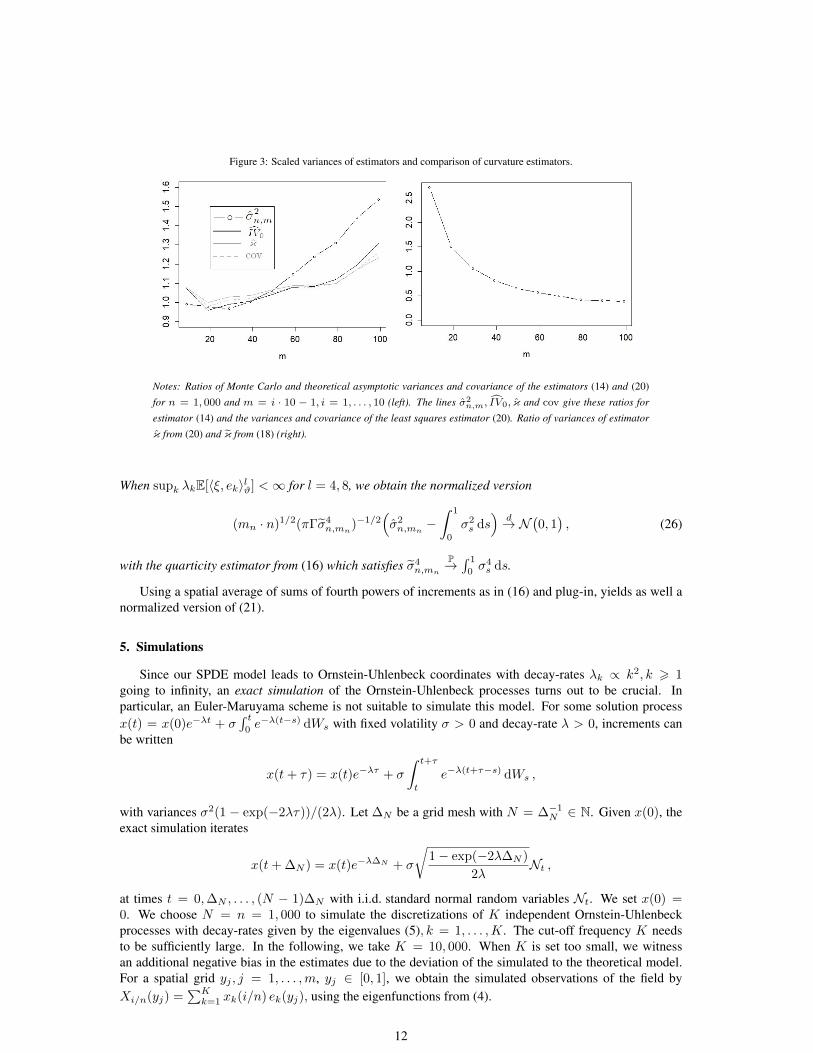
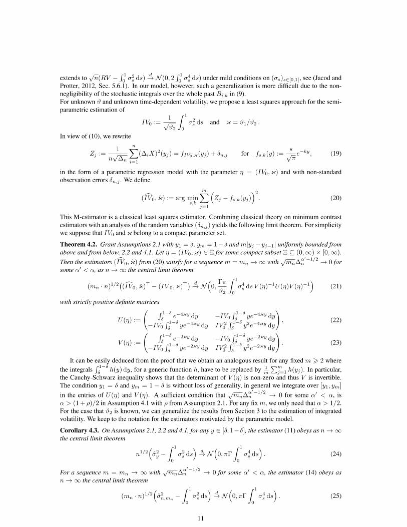
Figure 3: Scaled variances of estimators and comparison of curvature estimators.

Notes: Ratios of Monte Carlo and theoretical asymptotic variances and covariance of the estimators (14) and (20)for n = 1, 000 and m = i · 10 − 1, i = 1, . . . , 10 (left). The lines σ2

n,m, IV0, κ and cov give these ratios for

estimator (14) and the variances and covariance of the least squares estimator (20). Ratio of variances of estimator

κ from (20) and κ from (18) (right).

When supk λkE[〈ξ, ek〉lϑ] <∞ for l = 4, 8, we obtain the normalized version

(mn · n)1/2(πΓσ4n,mn)−1/2

(σ2n,mn −

∫ 1

0

σ2s ds

)d→ N

(0, 1), (26)

with the quarticity estimator from (16) which satisfies σ4n,mn

P→∫ 1

0σ4s ds.

Using a spatial average of sums of fourth powers of increments as in (16) and plug-in, yields as well anormalized version of (21).

5. Simulations

Since our SPDE model leads to Ornstein-Uhlenbeck coordinates with decay-rates λk ∝ k2, k > 1going to infinity, an exact simulation of the Ornstein-Uhlenbeck processes turns out to be crucial. Inparticular, an Euler-Maruyama scheme is not suitable to simulate this model. For some solution processx(t) = x(0)e−λt + σ

∫ t0e−λ(t−s) dWs with fixed volatility σ > 0 and decay-rate λ > 0, increments can

be written

x(t+ τ) = x(t)e−λτ + σ

∫ t+τ

t

e−λ(t+τ−s) dWs ,

with variances σ2(1 − exp(−2λτ))/(2λ). Let ∆N be a grid mesh with N = ∆−1N ∈ N. Given x(0), the

exact simulation iterates

x(t+ ∆N ) = x(t)e−λ∆N + σ

√1− exp(−2λ∆N )

2λNt ,

at times t = 0,∆N , . . . , (N − 1)∆N with i.i.d. standard normal random variables Nt. We set x(0) =0. We choose N = n = 1, 000 to simulate the discretizations of K independent Ornstein-Uhlenbeckprocesses with decay-rates given by the eigenvalues (5), k = 1, . . . ,K. The cut-off frequency K needsto be sufficiently large. In the following, we take K = 10, 000. When K is set too small, we witnessan additional negative bias in the estimates due to the deviation of the simulated to the theoretical model.For a spatial grid yj , j = 1, . . . ,m, yj ∈ [0, 1], we obtain the simulated observations of the field byXi/n(yj) =

∑Kk=1 xk(i/n) ek(yj), using the eigenfunctions from (4).

12

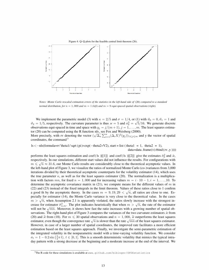
Figure 4: Q–Q plots for the feasible central limit theorem (26).

Notes: Monte Carlo rescaled estimation errors of the statistics in the left-hand side of (26) compared to a standard

normal distribution, for n = 1, 000 and m = 1 (left) and m = 9 equi-spaced spatial observations (right).

We implement the parametric model (3) with κ = 2/5 and σ = 1/4, or (1) with ϑ0 = 0, ϑ1 = 1 andϑ2 = 1/5, respectively. The curvature parameter is thus κ = 5 and σ2

0 =√

5/16. We generate discreteobservations equi-spaced in time and space with yj = j/(m+ 1), j = 1, . . . ,m. The least squares estima-tor (20) can be computed using the R function nls, see Fox and Weisberg (2000).More precisely, with rv denoting the vector (

√∆n

∑ni=1(∆iX)2(yj))16j6m and y the vector of spatial

coordinates, the command 3

ls<−nls(formula=rv˜theta1/ sqrt (pi)∗exp(−theta2∗V2), start = list ( theta1 = 1, theta2 = 1),data=data . frame(t ( rbind (rv ,y ))))

performs the least squares estimation and coef( ls )[[1]] and coef( ls )[[2]] give the estimates σ20 and κ,

respectively. In our simulations, different start values did not influence the results. For configurations withm 6

√n ≈ 31.6, our Monte Carlo results are considerably close to the theoretical asymptotic values. In

the left-hand plot of Figure 3, we visualize the ratios of normalized Monte Carlo (co-)variances from 3,000iterations divided by their theoretical asymptotic counterparts for the volatility estimator (14), which usesthe true parameter κ, as well as for the least squares estimator (20). The normalization is a multiplica-tion with factors mn, for fixed n = 1, 000 and for increasing values m = i · 10 − 1, i = 1, . . . , 10. Todetermine the asymptotic covariance matrix in (21), we compute means for the different values of m in(22) and (23) instead of the fixed integrals in the limit theorem. Values of these ratios close to 1 confirma good fit by the asymptotic theory. In the cases m = 9, 19, 29 <

√n, all ratios are close to one. Es-

pecially for estimator (14), the Monte Carlo variance is very close to the theoretical value. In the casesm >

√n, when Assumption 2.1 is apparently violated, the ratios slowly increase with the strongest in-

crease for estimator σ2n,m. The plot indicates heuristically that when m >

√n, the rate of the estimator

will not be√mn. Moreover, it shows how fast the ratio increases with a growing number of spatial ob-

servations. The right-hand plot of Figure 3 compares the variances of the two curvature estimators κ from(20) and κ from (18). For m 6 30 spatial observations and n = 1, 000, κ outperforms the least squaresestimator, even though the convergence rate

√n is slower than the rate

√mn of the least squares estimator.

However, in case of a larger number of spatial coordinates, the improved rate facilitates a more efficientestimation based on the least squares approach. Finally, we investigate the semi-parametric estimation ofthe integrated volatility in the nonparametric model with a time-varying volatility function. We considerσt = 1 − 0.2 sin

(34π t), t ∈ [0, 1]. This is a smooth deterministic volatility that mimics the typical intra-

day pattern with a strong decrease at the beginning and a moderate increase at the end of the interval. We

3The R-code for these simulations is available at www.github.com/bibinger/SPDEstatistics

13

analyze the finite-sample accuracy of the feasible central limit theorem (26). To this end, we rescale theestimation errors of estimator (14) with the square root of the estimated integrated quarticity, based onestimator (16), times

√Γπ. We compare these statistics rescaled with the rate

√mn from 3,000 Monte

Carlo iterations to the standard Gaussian limit distribution in the Q–Q plots in Figure 4 for n = 1, 000 andm = 1 and m = 9, respectively. The plots confirm a high finite-sample accuracy. In particular, the MonteCarlo empirical variances are very close to the ones predicted by the rate and the variance of the limit lawas long as m is of moderate size compared to n.

6. Proofs

6.1. Proof of Proposition 3.1 and Proposition 3.2

Before we prove the formula for the expected value of the squared increments, we need some auxiliarylemmas.

Lemma 6.1. On Assumptions 2.1 and 2.2, when σ is constant, there is a sequence (rn,i)16i6n satisfying∑ni=1 rn,i = O(∆

1/2n ) such that

E[(∆iX)2(y)] = σ2∑k>1

1− e−λk∆n

λk

(1− 1− e−λk∆n

2e−2λkti−1

)e2k(y) + rn,i . (27)

Proof. Recall Xt(y) =∑k>1 xk(t)ek(y) and (9). It holds that E[Ai,kBi,k] = E[Ai,kCi,k] =

E[Bi,kCi,k] = 0, as well as

E[A2i,k] = E

[〈ξ, ek〉2ϑ

]e−2λk(i−1)∆n(e−λk∆n − 1)2 , (28a)

E[B2i,k] =

∫ (i−1)∆n

0

σ2e−2λk((i−1)∆n−s)(e−λk∆n − 1)2 ds

= σ2(e−λk∆n − 1)2 1− e−2λk(i−1)∆n

2λk, (28b)

E[C2i,k] =

∫ i∆n

(i−1)∆n

σ2e−2λk(i∆n−s) ds =1− e−2λk∆n

2λkσ2 . (28c)

Since (Bi,k + Ci,k)k, k > 1, are independent and centered, we obtain

E[(∆iX)2(y)] =∑k,l>1

E[∆ixk∆ixl]ek(y)el(y)

= σ2∑k>1

(1− e−2λk∆n

2λk+(1− e−λk∆n

)2( 1

2λk(1− e−2λkti−1)

))e2k(y) + rn,i

= σ2∑k>1

(1− e−2λk∆n +(1− e−λk∆n

)22λk

−(e−λk∆n − 1

)22λk

e−2λkti−1

)e2k(y) + rn,i

= σ2∑k>1

1− e−λk∆n

λk

(1− 1− e−λk∆n

2e−2λkti−1

)e2k(y) + rn,i ,

where the remainder rn,i hinges on ξ and i:

rn,i =∑k,l>1

(1− e−λk∆n

)(1− e−λl∆n

)e−(λk+λl)ti−1E[〈ξ, ek〉ϑ〈ξ, el〉ϑ]ek(y)el(y) . (29)

14

If on Assumption 2.2 E[〈ξ, ek〉ϑ] = 0 and E[〈ξ, ek〉2ϑ] 6 C/λk with some C <∞, then we have that

rn,i 6 C∑k>1

(1− e−λk∆n

)2λk

e−2λkti−1e2k(y)

by independence of the coefficients. For the alternative condition from Assumption 2.2, we use that Aϑ isself-adjoint on Hϑ, such that −λ1/2

k 〈ξ, ek〉ϑ = 〈A1/2ϑ ξ, ek〉ϑ and thus

rn,i = E[(∑

k>1

1− e−λk∆n

λ1/2k

e−λkti−1ek(y)〈A1/2ϑ ξ, ek〉ϑ

)2].

The Cauchy-Schwarz inequality and Parseval’s identity yield that

rn,i 6∑k>1

(1− e−λk∆n)2

λke−2λkti−1e2

k(y)E[∑k>1

〈A1/2ϑ ξ, ek〉2ϑ

]6 2E

[‖A1/2

ϑ ξ‖2ϑ]∑k>1

(1− e−λk∆n)2

λke−2λk(i−1)∆n ,

where E[‖A1/2

ϑ ξ‖2ϑ]

is finite by assumption. We shall often use the elementary inequality

(1− p)(1− q)1− pq

6 1− p , for all 0 6 p, q < 1 . (30)

Applying this inequality and a Riemann sum approximation yields that

∑k>1

(1− e−λk∆n)2

λk

n∑i=1

e−2λk(i−1)∆n 6∑k>1

(1− e−λk∆n)2

λk(1− e−2λk∆n)

6 ∆n

∑k>1

(1− e−λk∆n)

λk∆n6 ∆1/2

n

∫ ∞0

1− e−z2

z2dz + O(∆1/2

n ) ,

such thatn∑i=1

rn,i = O(∆1/2n ) .

In order to evaluate the sums in the previous lemma, we apply the following result:

Lemma 6.2. If f : [0,∞) → R is twice continuously differentiable such that ‖f(x2)‖L1([0,∞)), ‖(1 ∨x)f ′(x2)‖L1([0,∞)), ‖(1 ∨ x2)f ′′(x2)‖L1([0,∞)) 6 C and |f(0)| 6 C for some C > 0, then:

(i)√

∆n

∑k>1

f(λk∆n) =

∫ ∞0

f(π2ϑ2z2) dz −

√∆n

2f(0) +O(∆n) and

(ii)√

∆n

∑k>1

f(λk∆n) cos(2πky) = −√

∆n

2f(0) +O

((δ−2∆n) ∧ (δ−1∆1/2

n ))

for any y ∈ [δ, 1− δ],

with δ from Assumption 2.1. The constant in the O-terms only depends on C.

Proof. We perform a substitution with z2 = k2∆n to approximate the sum by an integral, such that

λk∆n = z2 π2ϑ2 + ∆n

( ϑ21

4ϑ2− ϑ0

).

15

A Taylor expansion of f and using that f ′(x2) ∈ L1([0,∞)) shows that the remainder of setting λk∆n ≈π2z2ϑ2 is of order ∆n. A Riemann midpoint approximation yields for f(z) := f(π2ϑ2z

2), the gridak := ∆

1/2n (k + 1/2), k > 0, and intermediate points ξk ∈ [ak−1, ak] that

√∆n

∑k>1

f(λk∆n)−∫ ∞√

∆n2

f(π2ϑ2z2) dz =

∑k>1

∫ ak

ak−1

(f(√

∆nk)− f(z))

dz +O(∆n)

= −∑k>1

∫ ak

ak−1

((z − k

√∆n

)f ′(√

∆nk) +1

2

(z − k

√∆n

)2f ′′(ξk)

)dz +O(∆n)

= O(

∆n

∫ ∞0

|f ′′(z)|dz)

+O(∆n).

We have used a second-order Taylor expansion where the first-order term vanishes by symmetry. Sincef ′′ ∈ L1([0,∞)), we conclude that

√∆n

∑k>1

f(λk∆n) =

∫ ∞0

f(π2ϑ2z2) dz −

∫ √∆n2

0

f(π2ϑ2z2) dz +O(∆n).

The subtracted integral over the asymptotically small vicinity close to zero can be approximated byf(0)√

∆n/2 +O(∆n) concluding (i). To show (ii), we rewrite with Re denoting the real part of complexnumbers and i denoting the imaginary unit

√∆n

∑k>1

f(λk∆n) cos(2πky) =√

∆n

∑k>1

f(∆1/2n k) cos(2πky) +O(∆n)

= Re(√

∆n

∑k>1

f(∆1/2n k)e2πiky

)+O(∆n) .

Using (ak)k>0 from above, we derive that∫ ak

ak−1

e2πiuy/√

∆n du =

√∆n

2πiy

(e2πiaky/

√∆n − e2πiak−1y/

√∆n)

=

√∆n

2πiy

(eπiy − e−πiy

)e2πiky =

sin(πy)

πy

√∆ne

2πiky.

For a real-valued function f ∈ L1(R), we denote by F [f ] : R → C its Fourier transform F [f ](x) =∫f(t)e−ixt dt. In terms of the Fourier transform F , we obtain

√∆n

∑k>1

f(λk∆n) cos(2πky) = Re( πy

sin(πy)

∑k>1

f(∆1/2n k)

∫ ak

ak−1

e2πiuy/√

∆n du)

= Re( πy

sin(πy)F[∑k>1

f(∆1/2n k)1(ak−1,ak]

](−2πy∆−1/2

n ))

= T1 + T2,

where T1 := Re( πy

sin(πy)F[∑k>1

f(∆1/2n k)1(ak−1,ak] − f1(a0,∞)

](−2πy∆−1/2

n )),

T2 := Re( πy

sin(πy)F[f1(a0,∞)

](−2πy∆−1/2

n )).

Based on that decomposition, we first verify√

∆n

∑k>1 f(λk∆n) cos(2πky) = O(δ−1

√∆n). To bound

T1, a Riemann approximation yields

|T1| 6πy

sin(πy)

∥∥∥F[∑k>1

f(∆1/2n k)1(ak−1,ak] − f1(a0,∞)

]∥∥∥∞

16

6πy

sin(πy)

∥∥∥∑k>1

f(∆1/2n k)1(ak−1,ak] − f1(a0,∞)

∥∥∥L1

= O(δ−1∆1/2n ),

where we also have used that y is bounded away from 1 by δ.For the second term T2, we will use the decay of the Fourier transformation F [f ]. Since f ′, f ′′

∈ L1([0,∞)), we have |zF [f ](z)| = O(1) and |z2F [f ](z)| = O(1). Hence, for any y > δ > 0:

|F [f ](−2πy∆−1/2n )| = O

(√∆n

δ∧ ∆n

δ2

).

This implies that

T2 = −Re( πy

sin(πy)F [f1(0,a0]](−2πy∆−1/2

n ))

+O(√∆n

δ∧ ∆n

δ2

)= − πy

sin(πy)

∫ √∆n/2

0

cos(2πyu∆−1/2n )f(u) du+O

(√∆n

δ∧ ∆n

δ2

)= −∆

1/2n πy

sin(πy)

∫ 1/2

0

cos(2πyu)f(∆1/2n u) du+O

(√∆n

δ∧ ∆n

δ2

). (31)

In particular, we obtain |T2| = O(δ−1√

∆). Noting that the above estimates for T1, T2 apply to theimaginary part, too, we conclude

√∆n

∑k>1

f(λk∆n)g(2πky) = O(δ−1√

∆n) for g = cos or g = sin . (32)

To prove (ii), we tighten our bounds for T1, T2. For T1 we use a second-order Taylor expansion as for (i):

|T1| =∣∣∣Re

( πy

sin(πy)

∑k>1

∫ ak

ak−1

(f(∆1/2

n k)− f(z))e2πizy∆−1/2

n dz)∣∣∣

=πy

sin(πy)

∣∣∣Re(−∑k>1

∫ ak

ak−1

((z −∆1/2

n k)f ′(∆1/2n k) +

1

2(z −∆1/2

n k)2f ′′(ξk))e2πizy∆−1/2

n dz)∣∣∣

6πy

sin(πy)

∣∣∣∑k>1

∫ ak

ak−1

(z −∆1/2n k)f ′(∆1/2

n k) Re(e2πizy∆−1/2n )dz

∣∣∣+

πy

2 sin(πy)

(∑k>1

∫ ak

ak−1

(z −∆1/2n k)2|f ′′(ξk)|dz

)

=πy

sin(πy)

∣∣∣∑k>1

f ′(∆1/2n k)

∫ √∆n/2

−√

∆n/2

u cos(2π(u+ ∆1/2

n k)y∆−1/2n

)du∣∣∣+O

(δ−1∆n

∫ ∞0

|f ′′(z)|dz)

=πy

sin(πy)

∣∣∣∆n(πy cos(πy)− sin(πy))

2π2y2

∑k>1

f ′(∆1/2n k) sin(2πky)

∣∣∣+O(δ−1∆n

∫ ∞0

|f ′′(z)|dz),

where for the last equality, we compute the elementary integral. The sum in the last line is boundedsimilarly as in (32). Hence, |T1| = O(

√∆n

δ ∧ ∆n

δ2 ). For the second term T2, we apply integration by partsto (31) to obtain

T2 = −∆1/2n πy

sin(πy)

( sin(πy)

2πyf(∆1/2

n /2) + ∆1/2n

∫ 1/2

0

sin(2πyu)

2πyf ′(∆1/2

n u) du)

+O(√∆n

δ∧ ∆n

δ2

)= −1

2∆1/2n f(∆1/2

n /2) +O(√∆n

δ∧ ∆n

δ2

)= −1

2∆1/2n f(0) +O

(√∆n

δ∧ ∆n

δ2

).

Combining the estimates for T1 and T2 yields (ii).

17

Lemma 6.3. On Assumptions 2.1 and 2.2 it holds uniformly for all y ∈ [δ, 1− δ], δ > 0, that

E[(∆iX)2(y)] =√

∆nσ2e−y ϑ1/ϑ2

π√ϑ2

∫ ∞0

1− e−z2

z2

(1− 1− e−z2

2e−2z2(i−1)

)dz + rn,i +O(δ−2∆3/2

n ),

i ∈ {1, . . . , n}, where rn,i is the sequence from Lemma 6.1.

Proof. Inserting the eigenfunctions ek(y) from (5) and recalling that ti−1 = (i− 1)∆n, Lemma 6.1 givesfor i ∈ {1, . . . , n}

E[(∆iX)2(y)] = 2σ2∑k>1

1− e−λk∆n

λk

(1− 1− e−λk∆n

2e−2λk(i−1)∆n

)sin2(πky)e−y ϑ1/ϑ2 + rn,i .

Applying the identity sin2(z) = 1/2(1− cos(2z)), we decompose the sum into three parts, which will bebounded separately:

E[(∆iX)2(y)] = σ2√

∆n(I1 − I2(i) +R(i))e−y ϑ1/ϑ2 + rn,i , (33)

where I1 :=√

∆n

∑k>1

1− e−λk∆n

λk∆n, I2(i) :=

√∆n

∑k>1

(1− e−λk∆n

)22λk∆n

e−2λk(i−1)∆n ,

R(i) := −√

∆n

∑k>1

1− e−λk∆n

∆nλk

(1− 1− e−λk∆n

2e−2λk(i−1)∆n

)cos(2πky) .

The terms I1 and I2(i) can be approximated by integrals, determining the size of the expected squaredincrements. The remainder terms R(i) from approximating sin2 turn out to be negligible.

For I1 we apply Lemma 6.2(i) to the function f : [0,∞) → R, f(x) 7→ (1 − e−x)/x for x > 0 andf(0) = 1, and obtain

I1 =

∫ ∞0

(1− e−π2ϑ2z2

)

π2ϑ2z2dz −

√∆n

2+O(∆n) . (34)

For the second i-dependent term I2(i) in (33), we apply Lemma 6.2(i) to the functions

gi(x) =

{(1−e−x)2e−2x(i−1)

2x , x > 0 ,

0 , x = 0 ,

for 1 6 i 6 n. We obtain that

I2(i) =

∫ ∞0

gi(π2ϑ2z

2) dz +O(∆n) . (35)

Finally, for R(i) we use Lemma 6.2(ii) applied to

hi(x) =1− e−x

x

(1− (1− e−x)e−2x(i−1)

2

)for x > 0,

satisfying limx↓0 hi(x) = 1. We conclude R(i) = 12

√∆n +O(δ−2∆n).

With the above lemmas we can deduce Proposition 3.1.

Proof of Proposition 3.1. Computing the integrals in Lemma 6.3∫ ∞0

1− e−z2

z2dz =

√π ,

∫ ∞0

(1− e−z2

)2

z2e−2τz2

dz =√π(2√

1 + 2τ −√

2τ −√

2(1 + τ))

18

for any τ ∈ R, we derive that

E[(∆iX)2(y)] =√

∆n e−y ϑ1/ϑ2σ2

√1

ϑ2π

(1−

√1 + 2(i− 1) +

1

2

√2(i− 1) +

1

2

√2 + 2(i− 1)

)+ rn,i +O(∆3/2

n ) .

Since for the i-dependent term, by a series expansion we have that

n∑i=1

(√1 + 2(i− 1)− 1

2

√2(i− 1)− 1

2

√2 + 2(i− 1)

)= O

( n∑i=1

i−3/2), (36)

where the latter sum converges, we obtain

1

n

n∑i=1

e−y ϑ1/ϑ2σ2

√1

ϑ2π

(1−

√1 + 2(i− 1) +

1

2

√2(i− 1) +

1

2

√2 + 2(i− 1)

)= e−y ϑ1/ϑ2

√1

ϑ2πσ2 +O(∆n).

Since also the remainders from Lemmas 6.1 and 6.3 are bounded uniformly in i with the claimed rate, weobtain the assertion.

Next, we prove the decay of the covariances.

Proof of Proposition 3.2. Let us first calculate correlations between the terms Bi,k and Ci,k, which arerequired frequently throughout the following proofs.

ΣB,kij = Cov(Bi,k, Bj,k) = σ2(e−λk∆n − 1)2

∫ (min(i,j)−1)∆n

0

e−λk((i+j−2)∆n−2s) ds (37a)

=(e−λk|i−j|∆n − e−λk(i+j−2)∆n

) (e−λk∆n − 1)2

2λkσ2 ,

ΣC,kij = Cov(Ci,k, Cj,k) = 1{i=j} σ2 1− e−2λk∆n

2λk, (37b)

ΣBC,kij = Cov(Ci,k, Bj,k) = 1{i<j} σ2(e−λk∆n − 1)

∫ i∆n

(i−1)∆n

e−λk((i+j−1)∆n−2s) ds (37c)

= 1{i<j}(e−λk(j−i−1)∆n − e−λk(j−i+1)∆n

) (e−λk∆n − 1)

2λkσ2

= 1{i<j} e−λk(j−i)∆n

(eλk∆n − e−λk∆n

) (e−λk∆n − 1)

2λkσ2 .

The indicator 1{i<j} in (37b) reflects that E[Ci,kBj,k] = 0 whenever i > j. Since the Ornstein-Uhlenbeckprocesses (xk)k>1 are mutually independent, covariances between terms with k 6= l vanish. Note also theindependence between Ai,k and all Bi,k and Ci,k.Without loss of generality, consider Cov

(∆iX(y),∆jX(y)

)for j > i. Decompose increments as in (9):

Cov(∆iX(y),∆jX(y)

)=∑k>1

Cov(∆ixk,∆jxk) e2k(y)

=∑k>1

Cov(Ai,k +Bi,k + Ci,k, Aj,k +Bj,k + Cj,k) e2k(y)

= ri,j +∑k>1

(ΣB,kij + ΣBC,kij

)e2k(y)

19

with ΣB,kij and ΣBC,kij from (37a) and (37c) and with

ri,j =∑k>1

Var(〈ξ, ek〉ϑ

)e−λk(i+j−2)∆n(e−λk∆n − 1)2 e2

k(y)

6 2 supk

E[〈A1/2ϑ ξ, ek〉2ϑ]

∑k>1

(e−λk∆n − 1)2

λke−λk(i+j−2)∆n .

Using analogous steps as in the proof of Proposition 3.1, we derive that

Cov(∆iX(y),∆jX(y)

)=∑k>1

(ΣB,kij + ΣBC,kij

)e2k(y) + ri,j

=∑k>1

e−λk(j−i)∆nσ2 (e−λk∆n − 1)2 + 1− eλk∆n − e−2λk∆n + e−λk∆n

2λke2k(y)

−∑k>1

e−λk(j+i−2)∆nσ2 (e−λk∆n − 1)2

2λke2k(y)︸ ︷︷ ︸

=:si,j

+ri,j

=∑k>1

e−λk(j−i)∆nσ2

(2− e−λk∆n − eλk∆n

)2λk

e2k(y) + si,j + ri,j

=∑k>1

e−λk(j−i−1)∆nσ2

(2e−λk∆n − e−2λk∆n − 1

)2λk

e2k(y) + si,j + ri,j

= −∆1/2n

√∆n

∑k>1

e−λk(j−i−1)∆nσ2

(e−λk∆n − 1

)22λk∆n

e2k(y) + si,j + ri,j . (38)

Using the same approximation based on the equality sin2(z) = 12 − cos(2z) as in Lemma 6.3 combined

with the Riemann sum approximations from Lemma 6.2, the previous line equals

−∆1/2n exp(−y ϑ1/ϑ2)

σ2

2π√ϑ2

∫ ∞0

(1− e−z2)2

z2e−z

2(j−i−1) dz + si,j + ri,j +O(∆3/2n )

=−∆1/2n exp(−y ϑ1/ϑ2)

σ2

2√πϑ2

(2√j − i−

√j − i− 1−

√j − i+ 1

)+ si,j + ri,j +O(∆3/2

n ) .

The claim is implied by the estimaten∑

i,j=1

(si,j + ri,j) 6(σ2 + 2 sup

kE[〈A1/2

ϑ ξ, ek〉2ϑ]) n∑i,j=1

∑k>1

e−λk(j+i−2)∆n(e−λk∆n − 1)2

λk

=(σ2 + 2 sup

kE[〈A1/2

ϑ ξ, ek〉2ϑ])∑k>1

(e−λk∆n − 1)2

λk

( n−1∑i=0

e−λki∆n

)2

6(σ2 + 2 sup

kE[〈A1/2

ϑ ξ, ek〉2ϑ])∑k>1

(e−λk∆n − 1)2

λk(1− e−λk∆n)−2 = O(1).

6.2. Proofs of the central limit theoremsWe establish the central limit theorems based on a general central limit theorem for ρ-mixing triangular

arrays by Utev (1990, Thm. 4.1). More precisely, we use a version of Utev’s theorem where the mixingcondition is replaced by explicit assumptions on the partial sums that has been reported by Peligrad andUtev (1997, Theorem B). Set

ζn,i :=

√ϑ2π√m

m∑j=1

(∆iX)2(yj) exp(yj ϑ1/ϑ2) , (39)

20

where we consider either m = 1 or m = mn for a sequence satisfying mn = O(nρ) for some ρ ∈ (0, 1/2)according to Assumption 2.1.

If ξ is distributed according to the stationary distribution, i.e. the independent coefficients satisfy〈ξ, ek〉ϑ ∼ N (0, σ2/(2λk)), we have the representation ∆iX(y) =

∑k>1 ∆ixkek(y) with

∆ixk = Ci,k + Bi,k, Bi,k =

∫ (i−1)∆n

−∞σ(e−λk∆n − 1)e−λk((i−1)∆n−s)dW k

s , (40)

extending (W k)k>1 to Brownian motions on the whole real line for each k defined on a suitable extensionof the probability space. Note that ∆iX(y) is centered, Gaussian and stationary.

As the following lemma verifies, under Assumption 2.2 it is sufficient to establish the central limittheorems for the stationary sequence

ζn,i =

√ϑ2π√m

m∑j=1

(∆iX)2(yj) exp(yj ϑ1/ϑ2) . (41)

Lemma 6.4. On Assumptions 2.1 and 2.2, we have

n∑i=1

(ζn,i − ζn,i)P→ 0 .

Proof. It suffices to show that we have uniformly in y

√m

n∑i=1

((∆iX)2(y)− (∆iX)2(y)

) P→ 0 . (42)

By the decomposition (9), where we write Ai,k in the stationary case such that Ai,k + Bi,k = Bi,k, weobtain that

(∆iX)2(y)− (∆iX)2(y) =∑k,l

(∆ixk∆ixl −∆ixk∆ixl

)ek(y)el(y) = Ti − Ti

with Ti :=∑k,l

(Ai,kAi,l+Ai,k(Bi,l+Ci,l)+Ai,l(Bi,k+Ci,k)

)ek(y)el(y), and an analogous definition

of Ti where Ai,k and Ai,l are replaced by Ai,k and Ai,l, respectively. We show that√m∑ni=1 Ti

P→ 0under Assumption 2.2. Since this assumption is especially satisfied under the stationary initial distribution,we then conclude

√m∑ni=1 Ti

P→ 0 implying (42). To show that√m∑ni=1 Ti

P→ 0, we further separate

n∑i=1

Ti =

n∑i=1

(∑k>1

Ai,kek(y))2

+ 2

n∑i=1

(∑k>1

Ai,kek(y))(∑

k>1

(Bi,k + Ci,k)ek(y)). (43)

We have that

E[ n∑i=1

(∑k>1

Ai,kek(y))2]

6 2E[ n∑i=1

∑k>1

A2i,k

]+ E

[∣∣∣ n∑i=1

∑k 6=l

Ai,kAi,lek(y)el(y))∣∣∣2]1/2

Denoting Cξ := supk λkE[〈ξ, ek〉2ϑ], with (30), we obtain for the first term:

n∑i=1

∑k>1

E[A2i,k

]=

n∑i=1

∑k>1

(1− e−λk∆n)2e−2λk(i−1)∆nE[〈ξ, ek〉2ϑ

]6 Cξ

∑k>1

(1− e−λk∆n)2

λk

n∑i=1

e−2λk(i−1)∆n

21

6 Cξ∑k>1

(1− e−λk∆n)2

λk(1− e−2λk∆n)6 Cξ

∑k>1

(1− e−λk∆n)

λk= O(∆1/2

n ).

For the second term we have to distinguish between the case E[〈ξ, ek〉ϑ] = 0 in Assumption 2.2 (i), in thatwe can bound

n∑i,j=1

∑k 6=l

E[Ai,kAi,lAj,kAj,l

]=

n∑i,j=1

∑k 6=l

(1− e−λl∆n)2(1− e−λk∆n)2e−2(λk+λl)(i+j−2)∆nE[〈ξ, ek〉2ϑ

]E[〈ξ, el〉2ϑ

]6 C2

ξ

∑k,l>1

(1− e−λk∆n)2(1− e−λl∆n)2

λkλl(1− e−(λk+λl)∆n)26 C2

ξ

∑k,l>1

(1− e−λk∆n)(1− e−λl∆n)

λkλl= O(∆n),

using Assumption 2.2 (ii), the geometric series and inequality (30), and the second case in Assumption 2.2(i) where by Parseval’s identity C ′ξ :=

∑k λkE[〈ξ, ek〉2ϑ] < ∞. Under this condition we have an upper

boundn∑

i,j=1

∑k 6=l,k′ 6=l′

E[Ai,kAi,lAj,k′Aj,l′

]6( n∑i=1

(∑k>1

(1− e−λk∆n)e−λk(i−1)∆nE[〈ξ, ek〉2ϑ

]1/2)2)2

6( n∑i=1

(∑k>1

(1− e−λk∆n)2e−2λk(i−1)∆n

λk

)(∑k>1

λkE[〈ξ, ek〉2ϑ

]))2

6 C ′2ξ

(∑k>1

(1− e−λk∆n)2

λk(1− e−2λk∆n)

)2

= O(∆n).

The last term is of the same structure as the one in the last step of Lemma 6.1 from where we readily obtainthat it is O(∆n). Hence, Markov’s inequality yields that

∑ni=1(

∑k Ai,kek(y))2 = OP(∆

1/2n ). To bound

the second term in (43), we use independence of the terms Aj,k and (Bi,k + Ci,k) to obtain

E[∣∣∣ n∑i=1

(∑k>1

Ai,kek(y))(∑

k>1

(Bi,k + Ci,k)ek(y))∣∣∣2]

=

n∑i,j=1

(∑k>1

E[Ai,kAj,k]e2k(y)

)(∑k>1

E[(Bi,k + Ci,k)(Bj,k + Cj,k)

]e2k(y)

)=:

n∑i,j=1

Ri,jSi,j .

The first factor is bounded by

Ri,j =∑k>1

E[Ai,kAj,k]e2k(y) 6 2Cξ

∑k>1

(1− e−λk∆n)2

λke−λk(i+j−2)∆n ,

and satisfies supi,j |Ri,j | = O(∆1/2n ), as well as supj

∑i |Ri,j | = O(∆

1/2n ). The off-diagonal elements

with i < j of the second factor Si,j have been calculated in the proof of Proposition 3.2:

Si,j =∑k>1

(ΣB,kij + ΣBC,kij + ΣBC,kji + ΣC,kij

)e2k(y) =

∑k>1

(ΣB,kij + ΣBC,kij

)e2k(y)

6√

∆nσ2e−

yϑ1ϑ2

2√πϑ2

(2√j− i−

√j− i− 1−

√j− i+ 1

)+∑k>1

(1− e−λk∆n)2

λke−λk(i+j−2)∆n+O(∆3/2

n )

22

for i < j, while we obtain for i = j that

Si,i =∑k>1

(ΣB,kii + ΣC,kii

)e2k(y) 6 2σ2

∑k>1

( (1− e−λk∆n)2

2λk+

1− e−2λk∆n

2λk

)= 2σ2

∑k>1

1− e−λk∆n

λk.

Therefore, the second term in (43) has a second moment bounded by a constant times

n∑i,j=1

(∑k>1

(1− e−λk∆n)2

λke−λk(i+j−2)∆n

)(∆1/2n 1{i6=j}|j − i|−3/2

+∑k>1

(1{i=j}

1− e−λk∆n

λk+

(1− e−λk∆n)2

λke−λk(i+j−2)∆n

)+O(∆3/2

n ))

= O(

∆n

∑j>1

j−3/2 + ∆n

)= O(∆n).

We conclude that both terms in (43) are of the order OP(∆1/2n ) and thus that

√m∑ni=1 Ti

P→ 0 underAssumption 2.1. This implies (42).

Thanks to the previous lemma we can throughout investigate the solution process under the stationaryinitial condition. To prepare the central limit theorems, we compute the asymptotic variances in the nextstep. According to (11), we define the rescaled realized volatility at y ∈ (0, 1) based on the first p 6 nincrements as

Vp,∆n(y) :=

1

p√

∆n

p∑i=1

(∆iX)2(y)ey ϑ1/ϑ2 . (44)

Proposition 6.5. On Assumptions 2.1 and 2.2, the covariance of the rescaled realized volatility for twospatial points y1, y2 ∈ [δ, 1− δ] satisfies for any η ∈ (0, 1)

Cov(Vp,∆n

(y1), Vp,∆n(y2)

)= 1{y1=y2}p

−1Γσ4ϑ−12

(1 +O(1 ∧ (p−1∆η−1

n )))

(45)

+O(∆

1/2n

p(1{y1 6=y2}|y1 − y2|−1 + δ−1)

)where Γ > 0 is a numerical constant given in (52) with Γ ≈ 0.75. In particular, we have Var(Vn,∆n

(y)) =n−1Γσ4ϑ−1

2 (1 +O(√

∆n)).

Proof. Since

(∆iX)2(y) =(∑k>1

∆ixkek(y))2

=∑k,l

∆ixk∆ixlek(y)el(y),

we obtain the following variance-covariance structure of the rescaled realized volatilities (44) in pointsy1, y2 ∈ [δ, 1− δ]:

Cov(Vp,∆n(y1), Vp,∆n(y2)

)=e(y1+y2)ϑ1/ϑ2

∆np2

p∑i,j=1

( ∑k,l>1

ek(y1)ek(y2)el(y1)el(y2)Cov(∆ixk∆ixl,∆j xk∆j xl)

)

=e(y1+y2)ϑ1/ϑ2

∆np

∑k,l>1

ek(y1)ek(y2)el(y1)el(y2)Dk,l with

Dk,l =1

p

p∑i,j=1

Cov((Bi,k + Ci,k)(Bi,l + Ci,l), (Bj,k + Cj,k)(Bj,l + Cj,l)

),

23

while other covariances vanish by orthogonality. We will thus need the covariances of the terms in thedecomposition from (40) corresponding to (37a) to (37c). Since

Bi,k = Bi,k + σ(e−λ∆n − 1)√

2λkeλk(i−1)∆nZk

for a sequence of independent standard normal random variables (Zk)k>1, we find that

Cov(Bj,k, Ci,k) = Cov(Bj,k, Ci,k) = ΣBC,kij ,

Cov(Bi,k, Bj,k) = (2λk)−1 σ2(e−λk∆n − 1)2e−λk|i−j|∆n =: ΣB,kij . (46)

We deduce from Isserlis’ theorem

Dk,l =2

p

p∑i,j=1

(ΣB,kij + ΣBC,kij + ΣBC,kji + ΣC,kij

)(ΣB,lij + ΣBC,lij + ΣBC,lji + ΣC,lij

). (47)

In order to calculate Dk,l, we first study the case k < l and consider the different addends consecutively.Using (46), we derive that

1

p

p∑i,j=1

ΣB,kij ΣB,lij = σ4 (e−λk∆n − 1)2(e−λl∆n − 1)2

4λkλl

1 + e−(λk+λl)∆n

1− e−(λk+λl)∆n(48a)

×(

1 +O( p−1

1− e−(λk+λl)∆n

))exploiting the well-known formula for the geometric series, that we have for any q > 0

p∑i,j=1

q|i−j| = 2

p∑i=1

i−1∑j=1

qi−j + p = p1 + q

1− q+ 2

qp+1 − q(q − 1)2

,

which gives for q = exp(−(λk + λl)∆n) that

1

p

p∑i,j=1

e−(λk+λl)|i−j|∆n =1 + e−(λk+λl)∆n

1− e−(λk+λl)∆n

(1 +O

(1 ∧ p−1

1− e−(λk+λl)∆n

)).

Using (37b), we obtain that

1

p

p∑i,j=1

ΣC,kij ΣC,lij = σ4 (1− e−2λk∆n)(1− e−2λl∆n)

4λkλl. (48b)

With (37c), we derive that

1

p

p∑i,j=1

ΣBC,kij ΣBC,lij = σ4 (e−λk∆n − 1)(e−λl∆n − 1)

4λkλl

(1− e−2λk∆n)(1− e−2λl∆n)

1− e−(λk+λl)∆n(48c)

×(

1 +O(

1 ∧ p−1

1− e−(λk+λl)∆n

))and analogously for ΣBC,kji ΣBC,lji , using the auxiliary calculation:

1

p

p∑i=1

p∑j=i+1

(eλk∆n − e−λk∆n)(eλl∆n − e−λl∆n)e−(λk+λl)(j−i)∆n

= (eλk∆n − e−λk∆n)(eλl∆n − e−λl∆n)p−1

p∑i=1

e−(λk+λl)∆n − e−(λk+λl)(p−i+1)∆n

1− e−(λk+λl)∆n

24

= (eλk∆n − e−λk∆n)(eλl∆n − e−λl∆n)e−(λk+λl)∆n

1− e−(λk+λl)∆n

(1 +O

(1 ∧ p−1

1− e−(λk+λl)∆n

))=

(1− e−2λk∆n)(1− e−2λl∆n)

1− e−(λk+λl)∆n

(1 +O

(1 ∧ p−1

1− e−(λk+λl)∆n

)).

For the mixed terms, we infer that

1

p

p∑i,j=1

ΣB,kij

(ΣBC,lij + ΣBC,lji

)= σ4 (e−λk∆n − 1)2(e−λl∆n − 1)

2λkλle−λk∆n

1− e−2λl∆n

1− e−(λk+λl)∆n(48d)

×(

1 +O(

1 ∧ p−1

1− e−(λk+λl)∆n

)),

1

p

p∑i,j=1

ΣB,kij ΣC,lij = σ4 (e−λk∆n − 1)2(1− e−2λl∆n)

4λkλl, (48e)

1

p

p∑i,j=1

ΣC,kij ΣBC,lij =1

p

p∑i,j=1

ΣBC,kij ΣC,lij =1

p

p∑i,j=1

ΣBC,kij ΣBC,lji = 0 , (48f)

based on (37a)-(37c) and similar ingredients as above. With (48a)-(48f), we obtain that Dk,l, k < l, from(47) is given by σ4(1 +O(1 ∧ p−1

1−e−(λk+λl)∆n)) times

2

((e−λk∆n − 1)2(e−λl∆n − 1)2

4λkλl

1 + e−(λk+λl)∆n

1− e−(λk+λl)∆n+

(1− e−2λk∆n)(1− e−2λl∆n)

4λkλl

+(e−λk∆n − 1)(e−λl∆n − 1)

2λkλl

(1− e−2λk∆n)(1− e−2λl∆n)

1− e−(λk+λl)∆n

+(e−λk∆n − 1)2(e−λl∆n − 1)

2λkλle−λk∆n

1− e−2λl∆n

1− e−(λk+λl)∆n+

(e−λk∆n − 1)2(1− e−2λl∆n)

4λkλl

+(e−λl∆n − 1)2(1− e−2λk∆n)

4λkλl+

(e−λl∆n − 1)2(e−λk∆n − 1)

2λkλle−λl∆n

1− e−2λk∆n

1− e−(λk+λl)∆n

)=

(1− e−λk∆n)2(1− e−λl∆n)2

2λkλl

3− e−(λk+λl)∆n

1− e−(λk+λl)∆n

+(1− e−2λk∆n)(1− e−2λl∆n)

2λkλl+

(1− e−λk∆n)2(1− e−2λl∆n)

2λkλl+

(1− e−λl∆n)2(1− e−2λk∆n)

2λkλl

=(1− e−λk∆n)2(1− e−λl∆n)2

2λkλl

4− 2e−(λk+λl)∆n

1− e−(λk+λl)∆n

+(1− e−λk∆n)(1− e−λl∆n)

2λkλl

(− (1− e−λk∆n)(1− e−λl∆n) + (1 + e−λk∆n)(1 + e−λl∆n)

+ (1− e−λk∆n)(1 + e−λl∆n) + (1 + e−λk∆n)(1− e−λl∆n))

=(1− e−λk∆n)2(1− e−λl∆n)2

λkλl

2− e−(λk+λl)∆n

1− e−(λk+λl)∆n

+(1− e−λk∆n)(1− e−λl∆n)

λkλl

(2− (1− e−λk∆n)(1− e−λl∆n)

)=

(1− e−λk∆n)2(1− e−λl∆n)2

λkλl

1

1− e−(λk+λl)∆n+ 2

(1− e−λk∆n)(1− e−λl∆n)

λkλl=: Dk,l.

Since (1−e−(λk+λl)∆n)−1 6 (1−e−λk∆n)−1/2(1−e−λl∆n)−1/2, the remainder involving 1∧ p−1

1−e−(λk+λl)∆n

is negligible if p is sufficiently large:

1

∆np2

∑k<l

Dk,l

1− e−(λk+λl)∆n6

3

∆2np

2

(∆1/2n

∑k>1

(1− e−λk∆n)1/2

λk

)2

25

= O(∆η−1

n

p2

(∫ ∞0

(1− e−z2

)1/2

zη+1dz)2)

,

for any η ∈ (0, 1). For smaller p we can always obtain a bound of orderO(p−1). The diagonal terms k = lin (47) are bounded by

Dk,k 68

p

p∑i,j=1

((ΣB,kij

)2+ 2(ΣBC,kij

)2+(ΣC,kij

)2).

With estimates analogous to (48a), (48b) and (48c) we obtain 1∆np2

∑k>1Dk,k = O(∆

1/2n /p) which is

thus negligible. By symmetry Dk,l = Dl,k, we conclude

Cov(Vp,∆n

(y1), Vp,∆n(y2)

)=

2σ4e(y1+y2)ϑ1/ϑ2

∆np

∑k<l

ek(y1)ek(y2)el(y1)el(y2)Dk,l (49)

+O(1

p

(∆1/2n + ∆η−1

n p−1 ∧ 1)).

To evaluate the main term, we use λk∆n > 0 for all k and thus exp(−(λk + λl)∆n) 6 1 implying

Dk,l =

∞∑r=0

(1− e−λk∆n)2(1− e−λl∆n)2

λkλle−r(λk+λl)∆n + 2

(1− e−λk∆n)(1− e−λl∆n)

λkλl.

In particular, each above addend has a product structure with respect to k, l. In case that y1 6= y2, theidentity

ek(y1)ek(y2) = 2 sin(πky1) sin(πky2)e−(y1+y2)ϑ1/(2ϑ2)

=(

cos(πk(y1 − y2))− cos(πk(y1 + y2)))e−(y1+y2)ϑ1/(2ϑ2) (50)

can be used to prove that covariances from (49) vanish asymptotically at first order. More precisely, ap-plying Lemma 6.2(ii) to fr(x) = (1 − e−x)2e−rx/x, x > 0, fr(0) = 0, (49) results, with z, z′ ∈{(y1 − y2)/2, (y1 + y2)/2}, in terms of the form

∆n

p

∑r>0

∑k,l

cos(2πkz) cos(2πlz′)fr(λk∆n)fr(λl∆n)

=1

p

∑r>0

(∆1/2n

∑k>1

fr(λk∆n) cos(2πkz))(

∆1/2n

∑l>1

fr(λl∆n) cos(2πlz′))

=O(∆

1/2n (|y1 − y2|−1 + δ−1)

p

∑r>0

∆1/2n

∑k

|fr(λk∆n)|)

=O(∆

1/2n (|y1 − y2|−1 + δ−1)

p

(∆1/2n

∑k>1

1− e−λk∆n

λk∆n

))= O

(∆1/2n (|y1 − y2|−1 + δ−1)

p

). (51)

We are thus left to consider for any y ∈ [δ, 1 − δ] the variance. Using again Lemma 6.2(ii), one canapproximate the terms e2

k(y) = 2 sin2(πky)e−y ϑ1/ϑ2 ≈ e−y ϑ1/ϑ2 for the variances with y1 = y2 = y, upto a term of orderO(δ−1

√∆n/p), similar to the calculation (51). Hence, all variances of the statistics (44)

are equal at first order and we find

Var(Vp,∆n(y)) =

σ4

∆np

∑k 6=l

Dk,l +O(1

p

(∆1/2n δ−1 + ∆η−1

n p−1 ∧ 1))

=σ4

∆np

( ∞∑r=0

(∑k>1

(1− e−λk∆n)2e−rλk∆n

λk

)2

+ 2(∑k>1

1− e−λk∆n

λk

)2)

+O(1

p

(∆1/2n δ−1 + ∆η−1

n p−1 ∧ 1)),

26

using again that the diagonal terms k = l are negligible. To evaluate the leading term, we now apply theintegral approximations of the Riemann sums. For r ∈ N we have

lim∆n→0

∆1/2n

∑k>1

(1− e−λk∆n)2e−rλk∆n

λk∆n=

1√ϑ2π

∫ ∞0

(1− e−x2

)2e−rx2

x2dx

=1√ϑ2π

(2√r + 1−

√r + 2−

√r)

=:

√1

πϑ2I(r),

lim∆n→0

∆1/2n

∑k>1

1− e−λk∆n

λk∆n=

1√ϑ2π

∫ ∞0

1− e−x2

x2dx =

√1

πϑ2.

Hence,

Var(Vp,∆n(y)) =1

p

σ4

πϑ2

( ∞∑r=0

I(r)2 + 2)

+O(δ−1∆

1/2n

p+

1

p∧ ∆η−1

n

p2

).

Since the series above converges, we obtain (45) with the constant

Γ :=1

π

∞∑r=0

I(r)2 +2

π(52)

with I(r) = 2√r + 1−

√r + 2−

√r. To evaluate Γ numerically, we rely on the series approximation

∞∑r=0

I(r)2 ≈ 0.357487 and thus Γ ≈ 1

π

(0.357487 + 2

)≈ 0.75 .

Before we prove the central limit theorems we provide a result that will be used to verify the generalizedmixing-type condition.

Proposition 6.6. For y ∈ (0, 1), and natural numbers 1 6 r < r + u 6 v 6 n, and

Qr1 =

r∑i=1

(∆iX)2(y), Qvr+u =

v∑i=r+u

(∆iX)2(y) , (53)

there exists a constant C, 0 < C <∞, such that for all t ∈ R∣∣Cov(eit(Qr1−E[Qr1]), eit(Qvr+u−E[Qvr+u]))∣∣ 6 C t2

u3/4Var(Qr1)1/2Var

(Qvr+u

)1/2.

Proof. For brevity we write Y = Y − E[Y ] for random variables Y . For any decomposition Qvr+u =A1 +A2, with some A2 which is independent of Qr1, we have

Cov(eitQr1 , eitQvr+u) = Cov(eitQr1 − 1, eitQvr+u)

= E[(eitQr1 − 1)eitA2(eitA1 − 1)

]+ E

[eitQr1 − 1

]E[eitA2(1− eitA1)

].

Using that |eix − 1| 6 |x| and |eix| = 1, x ∈ R, we thus get∣∣Cov(eitQr1 , eitQvr+u)∣∣ 6 E[|tQr1| |tA1|] + E[|tQr1|]E[|tA1|] 6 2t2E[(Qr1)2]1/2E[A2

1]1/2 , (54)

by the Cauchy-Schwarz and Jensen’s inequality. To obtain such a decomposition, we write for i > r

∆iX(y) =∑k>1

Dk,i1 ek(y) +

∑k>1

Dk,i2 ek(y), where (55)

Dk,i1 :=

∫ r∆n

−∞e−λk((i−1)∆n−s)(e−λk∆n − 1)σ dW k

s ,

27

Dk,i2 :=

∫ (i−1)∆n

r∆n

e−λk((i−1)∆n−s)(e−λk∆n − 1)σ dW ks +

∫ i∆n

(i−1)∆

e−λk(i∆n−s)σdW ks .

Then we can decompose

Qvr+u =

v∑i=r+u

(∆iX)2(y) =

v∑i=r+u

(∑k>1

Dk,i1 ek(y)

)2

+ 2

v∑i=r+u

(∑k>1

Dk,i1 ek(y)

)(∑k>1

Dk,i2 ek(y)

)︸ ︷︷ ︸

=:A1

+

v∑i=r+u

(∑k>1

Dk,i2 ek(y)

)2

︸ ︷︷ ︸=:A2

.

We bound E[A21] = Var(A1) by

E[A21] 6 E[A2

1] =

v∑i,j=r+u

(E[(∑

k>1

Dk,i1 ek(y)

)2(∑k>1

Dk,j1 ek(y)

)2]+ 4E

[(∑k>1

Dk,i1 ek(y)

)(∑k>1

Dk,i2 ek(y)

)(∑k>1

Dk,j1 ek(y)

)(∑k>1

Dk,j2 ek(y)

)])=: T1 + T2 ,

where the cross term vanishes by independence of Dk,i1 and Dk,j

2 . Set p := v − r − u + 1. SinceDk,i

1 = e−λk(i−r−1)∆nBr+1,k, with Br+1,k from (40), we have for u > 2 that

T1 =

v∑i,j=r+u

E[(∑

k>1

e−λk(i−r−1)∆nBr+1,kek(y))2(∑

k>1

e−λk(j−r−1)∆nBr+1,kek(y))2]

=

v∑i,j=r+u

∑k 6=l

E[B2r+1,k]E[B2

r+1,l](e−2λk(i−r−1)∆n−2λl(j−r−1)∆n + 2e−(λk+λl)(i+j−2r−2)∆n

)× e2

k(y)e2l (y) +

v∑i,j=r+u

∑k>1

E[B4r+1,k]e−2λk(i+j−2r−2)∆ne4

k(y)

= σ4∑k 6=l

(1− e−λk∆n)2(1− e−λl∆n)2

4λkλl

(( v∑i=r+u

e−2λk(i−r−1)∆n

)( v∑j=r+u

e−2λl(j−r−1)∆n

)+ 2( v∑i=r+u

e−(λk+λl)(i−r−1)∆n

)2)e2k(y)e2

l (y)

+ 3σ4∑k>1

(1− e−λk∆n)4

4λ2k

( v∑i=r+u

e−2λk(i−r−1)∆n

)2

e4k(y)

6 4σ4p∑k 6=l

(1− e−λk∆n)2(1− e−λl∆n)2

4λkλle−2(λk+λl)(u−1)∆n

( 1

(1− e−2λk∆n)+

2

(1− e−(λk+λl)∆n)

)+ 12σ4p

∑k>1

(1− e−λk∆n)4

4λ2k

e−4λk(u−1)∆n

(1− e−2λk∆n)

6 3σ4p(∑k>1

e−2λk(u−1)∆n1− e−λk∆n

λk

)(∑k>1

e−2λk(u−1)∆n(1− e−λk∆n)2

λk

),

where we use (46) and e2k(y) 6 2 for all k. For the last inequality we use (30) three times, once with

p = e−λk∆n and q = e−λl∆n , and twice with p = q = e−λk∆n . With the two integral bounds∫ ∞0

(1− e−z2

)j

z2e−2(u−1)z2

dz = O(u1/2−j) , for j = 1, 2 , (56)

28

we derive that for some constant C:T1 6 Cσ4 p∆n

(u− 1)2. (57)

For the second term, the independence of Dk,i1 and Dl,j

2 and the Cauchy-Schwarz inequality yield

T2 =

v∑i,j=r+u

E[(∑

k>1

Dk,i1 ek(y)

)(∑k>1

Dk,j1 ek(y)

)]E[(∑

k>1

Dk,i2 ek(y)

)(∑k>1

Dk,j2 ek(y)

)]=

v∑i,j=r+u

(∑k>1

E[Dk,i

1 Dk,j1

]e2k(y)

)(∑k>1

E[Dk,i

2 Dk,j2

]e2k(y)

).

For i 6 j, with (37b), (37c), and a term similar to (37a), we have that

E[Dk,i

2 Dk,j2

]=E[( ∫ (i−1)∆n

r∆n

e−λk((i−1)∆n−s)(e−λk∆n − 1)σ dW ks + Ci,k

)×(∫ (j−1)∆n

r∆n

e−λk((j−1)∆n−s)(e−λk∆n − 1)σ dW ks + Cj,k

)]=σ2(1− e−λk∆n)2e−λk(i+j−2)∆n

∫ (i−1)∆n

r∆n

e2λks ds+ ΣBC,kij + ΣC,kij

=σ2 (1− e−λk∆n)2

2λk

(e−λk(j−i)∆n − e−λk(i+j−2r−2)∆n

)+ ΣBC,kij + ΣC,kij ,

where the second addend is zero for i = j and the last one for i < j. By (37c), we especially observe fori < j that

E[Dk,i

2 Dk,j2

]= σ2 1− e−λk∆n

2λke−λk(j−i)∆n

((1− e−λk∆n)(1− e−2λk(i−r−1)∆n)− (eλk∆ − e−λk∆)

)6 σ2 1− e−λk∆n

2λke−λk(j−i)∆n

(1− eλk∆

)6 0.

Thereby and with (46), we obtain for u > 2 and some constant C that

T2 = σ4v∑

i=r+u

(∑k>1

e−2λk(i−r−1)∆n(1− e−λk∆n)2

2λke2k(y)

)×(∑k>1

( (1− e−λk∆n)2

2λk

(1− e−2λk(i−r−1)∆n

)+ ΣC,kii

)e2k(y)

)+ 2σ4

∑r+u6i<j6v

(∑k>1

e−λk(i+j−2r−2)∆n(1− e−λk∆n)2

2λke2k(y)

)(∑k>1

E[Dk,i

2 Dk,j2

]e2k(y)

)6 4σ4

v∑i=r+u

(∑k>1

e−2λk(i−r−1)∆n(1− e−λk∆n)2

2λk

)(∑k>1

(1− e−λk∆n)2 + 1− e−2λk∆n

2λk

)6 2σ4p

(∑k>1

e−2λk(u−1)∆n(1− e−λk∆n)2

λk

)(∑k>1

(1− e−λk∆n)

λk

)6 C

σ4p∆n

(u− 1)3/2.

For the last inequality, we use (56) and the same application of Lemma 6.2 as to I1 in (34). In combinationwith (57), we conclude for u > 2 that with some constant C:

E[A21] 6 C

σ4p∆n

(u− 1)3/2.

29

We finally note that

E[(Qvr+u

)2]= E

[( v∑i=r+u

(∆iX)2(y))2]

>v∑

i=r+u

E[(∆iX)4(y)

]> C ′′σ4p∆n

for some constant C ′′ > 0. Combining these estimates with (54), and a simple bound for the case u = 1,completes the proof.

Based on the two previous propositions, we now prove the central limit theorems.

Proof of Theorem 3.3. For m = 1, the random variables ζn,i from (41) simplify to

ζn,i =√ϑ2π(∆iX)2(y) exp(y ϑ1/ϑ2) ,

such that σ2y = 1

n√

∆n

∑ni=1 ζn,i. By Proposition 3.1 we have E[

∑ni=1 ζn,i] =

√nE[σ2

y] =√n(σ2+O(1)).

Therefore, we are left to establish a central limit theorem for the triangular array

Zn,i = ζn,i − E[ζn,i] .

According to Peligrad and Utev (1997, Thm. B), the weak convergence∑ni=1 Zn,i

d→ N (0, v2) withasymptotic variance v2 = limn→∞Var(

∑ni=1 Zn,i) <∞ holds under the following sufficient conditions:

Var( b∑i=a

Zn,i

)6 C

b∑i=a

Var(Zn,i) for all 1 6 a 6 b 6 n , (58a)

lim supn→∞

n∑i=1

E[Z2n,i] <∞, (58b)

n∑i=1

E[Z2n,i1|Zn,i|>ε]→ 0 as n→∞ , for all ε > 0 , (58c)

Cov(eit

∑bi=a Zn,i , eit

∑ci=b+u Zn,i

)6 ρt(u)

c∑i=a

Var(Zn,i) , (58d)

for all 1 6 a 6 b < b+ u 6 c 6 n, and t ∈ R ,

with a universal constant C > 0 and a function ρt(u) > 0 satisfying∑j>1 ρt(2

j) <∞.

Since∑ni=1 ζn,i = n

√∆nVn,∆n(y)

√ϑ2π, by Proposition 6.5 the asymptotic variance is

limn→∞

ϑ2π∆nn2Var(Vn,∆n(y)) = Γπσ4 = v2 .

Proposition 6.5 implies that Var(∑bi=a Zn,i) = O(∆n(b− a+ 1)). Since ∆iX(y) are centered normally

distributed random variables with Var(∆iX(y)) ∝ ∆1/2n uniformly in i owing to Proposition 3.1, there ex-

ists a constant c > 0, such that∑bi=aVar(Zn,i) > c(b−a+1)∆n. Thus, we have verified Condition (58a).

From Proposition 6.5 we also obtain that∑ni=1 Var(Zn,i) = O(∆nn), which grants Condition (58b). The

generalized mixing-type Condition (58d) is verified by Proposition 6.6.It remains to establish the Lindeberg Condition (58c) which is by Markov’s inequality implied by a

Lyapunov condition. Using again that ∆iX(y) are centered normally distributed with Var(∆iX(y)) =

O(∆1/2n ) uniformly in i, we conclude E

[(∆iX)8(y)

]= O(∆2

n) and thus E[ζ4n,i

]= O(∆2

n) uniformly ini. Therefore,

n∑i=1

E[Z4n,i

]= O(n∆2

n) = O(1) as n→∞ .

For the case of m > 1 spatial observations we need the following corollary from Proposition 6.6:

30

Corollary 6.7. Under the conditions of Theorem 3.4, for natural numbers 1 6 r < r + u 6 v 6 n, and

Qr1 =

r∑i=1

ζn,i, Qvr+u =

v∑i=r+u

ζn,i ,

with ζn,i from (41), there exists a constant C, 0 < C <∞, such that for all t ∈ R∣∣Cov(eit(Qr1−E[Qr1]), eit(Qvr+u−E[Qvr+u]))∣∣ 6 Ct2

u3/4Var(Qr1)1/2Var

(Qvr+u

)1/2.

Proof. With Dk,i1 and Dk,j

2 from (55) we decompose

Qvr+u =

v∑i=r+u

ζn,i =

√ϑ2π√m

m∑j=1

(A1(yj) +A2(yj)

)eyjϑ1/ϑ2 with

A1(y) :=

v∑i=r+u

(∑k>1

Dk,i1 ek(y)

)2

+ 2

v∑i=r+u

(∑k>1

Dk,i1 ek(y)

)(∑k>1

Dk,i2 ek(y)

),

A2(y) :=

v∑i=r+u

(∑k>1

Dk,i2 ek(y)

)2

and set p := v − r − u+ 1. In view of (54), we thus have to estimate

Var(m−1/2

m∑j=1

A1(yj))

=1

m

m∑j=1

Var(A1(yj)

)+

1

m

∑j 6=j′

Cov(A1(yj), A1(yj′)

).

The covariances can be handled using (50) together with Lemma 6.2(ii) as in the proof of Proposition 6.5.By an analogous computation to the bounds for T1 and T2 as in the proof of Proposition 6.6, using thatm ·minj=2,...,m |yj − yj−1| is bounded from below, we thus obtain for u > 2 that

1

m

∑j 6=j′

Cov(A1(yj), A1(yj′)

)= O

(∆

3/2n p

(u− 1)3/2

1

m

∑j 6=j′

1

|yj − yj′ |

)= O

(∆

3/2n p

(u− 1)3/2m logm

). (59)

On the other hand, Proposition 6.6 yields, with a constant C, that

1

m

m∑j=1

Var(A1(yj)

)6

Cσ4 p∆n

(u− 1)3/2.

Using that E[(Qvr+u

)2]> C ′′σ4p∆n completes the proof.

Proof of Theorem 3.4. Similar to the proof of Theorem 3.3 we verify the Conditions (58a) to (58d) forthe triangular array Zn,i = ζn,i − E[ζn,i], with ζn,i from (41), where m = mn is a sequence satisfyingmn = O(nρ) for some ρ ∈ (0, 1/2) according to Assumption 2.1.From the proof of Proposition 6.5, using that m · minj=2,...,m |yj − yj−1| is bounded from below byAssumption 2.1, we deduce for any 0 6 a < b 6 n, with a similar estimate to (59), that

Var( b∑i=a

ζn,i

)=∆n(b−a+1)Γσ4π

(1 +O(1 ∧∆−1/4

n /(b−a+1)))+O

((b−a+1)∆3/2

n m logm)

= O(∆n(b−a+1)

).

We conclude in particular Conditions (58a) and (58b). By the Cauchy-Schwarz inequality we moreoverhave that

E[ζ4n,i

]=π2ϑ2

2

m2

m∑j1,...,j4=1

e(yj1+···+yj4 )ϑ1/ϑ2E[(∆iX)2(yj1) · · · (∆iX)2(yj4)

]

31

6π2ϑ2

2

m2

m∑j1,...,j4=1

e(yj1+···+yj4 )ϑ1/ϑ2E[(∆iX)8(yj1)

]1/4 · · ·E[(∆iX)8(yj4)]1/4

6 π2ϑ22m

2e4ϑ1/ϑ2 maxy∈{y1,...,ym}

E[(∆iX)8(y)

]. (60)

Using as in the proof of Theorem 3.3 that E[(∆iX)8(y)

]= O(∆2

n), we obtain that∑ni=1 E

[ζ4n,i

]=

O(m2∆n) = O(1), such that a Lyapunov condition is satisfied implying the Lindeberg Condition (58c).Finally, the mixing-type Condition (58d) is verified by Corollary 6.7.

Proof of Proposition 3.5. First, we compute the expectation of the quarticity estimator. We have thatE[σ4

n,m] = σ4 + O(1), since for any y ∈ [δ, 1− δ]n∑i=1

πϑ2 exp(2y ϑ1/ϑ2)E[(∆iX)4(y)

]= πϑ2 exp(2y ϑ1/ϑ2)

n∑i=1

∑k,l

3E[(∆ixk)2]E[(∆ixl)2] e2

k(y)e2l (y)

(1 + O(1)

)= 3πϑ2∆n

n∑i=1

(∆−1/2n

∑k>1

(ΣB,kii + ΣC,kii

))2(1 + O(1)

)= 3nπϑ2∆n

(∆−1/2n σ2

∑k>1

λ−1k

(1− exp(−λk∆n)

))2(1 + O(1)

)= 3σ4

(1 + O(1)

).

We use that the fourth-moment terms of Ai,k from (9) are negligible under the condition thatsupk λkE[〈ξ, ek〉4ϑ] < ∞. Recall the statistic ζn,i from (39). In order to establish consistency of thequarticity estimator, observe that for j > i with generic constant C:

Cov(ζ2n,j , ζ

2n,i

)=π2ϑ2

2

m2

m∑u1,...,u4=1

e(yu1+···+yu4 )ϑ1/ϑ2

× Cov((∆iX)2(yu1

)(∆iX)2(yu2), (∆jX)2(yu3

)(∆jX)2(yu4))

6 π2ϑ22 e

4ϑ1/ϑ2 m2 maxu1,u2,u3,u4∈{1,...,m}

∣∣Cov((∆iX)2(yu1

)(∆iX)2(yu2), (∆jX)2(yu3

)(∆jX)2(yu4))∣∣

6 Cm2∑k,l,p,q

Cov(∆ixk∆ixl∆ixp∆ixq,∆jxk∆jxl∆jxp∆jxq

)= Cm2

∑k,l,p,q

(ΣB,kij + ΣBC,kij

)(ΣB,lij + ΣBC,lij

)(ΣB,pij + ΣBC,pij

)(ΣB,qij + ΣBC,qij

)(1 + O(1)

)= Cm2∆2

n

(∆−1/2n

∑k>1

(ΣB,kij + ΣBC,kij

))4 (1 + O(1)

)= O

(m2∆2

nσ8(∫ ∞

0

z−2(1− e−2z2

)2 e−z2(j−i−1) dz

)4)= O

(m2∆2

nσ8(2√j − i−

√j − i− 1−

√j − i+ 1

)4)= O

(m2∆2

nσ8(j − i− 1)−6

).

Here, we use that the terms with fourth and eighth moments of Ai,k are negligible under the conditionthat supk λkE[〈ξ, ek〉4ϑ] < ∞ and supk λkE[〈ξ, ek〉8ϑ] < ∞. With E

[ζ4n,i

]= O(m2∆2

n) and the order ofCov

(ζ2n,j , ζ

2n,i

)for i 6= j, we obtain that

Var( n∑i=1

ζ2n,i

)6

n∑i=1

E[ζ4n,i

]+∑i6=j

Cov(ζ2n,j , ζ

2n,i

)

32

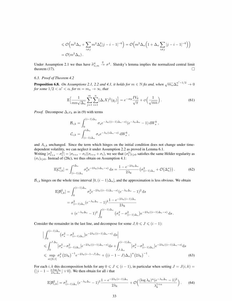
6 O(m2∆n +

∑i 6=j

m2∆2n|j − i− 1|−6

)= O

(m2∆n

(1 + ∆n

∑i 6=j

|j − i− 1|−6))

= O(m2∆n) .

Under Assumption 2.1 we thus have σ4n,m

P→ σ4. Slutsky’s lemma implies the normalized central limittheorem (17).

6.3. Proof of Theorem 4.2

Proposition 6.8. On Assumptions 2.1, 2.2 and 4.1, it holds for m ∈ N fix and, when√mn∆

α′−1/2n → 0

for some 1/2 < α′ < α, for m = mn →∞, that

E[ 1

mn√

∆n

m∑j=1

n∑i=1

(∆iX)2(yj)]

= e−κyIV0√π

+ O( 1√

mn

). (61)

Proof. Decompose ∆ixk as in (9) with terms

Bi,k =

∫ (i−1)∆n

0

σse−λk((i−1)∆n−s)(e−λk∆n − 1) dW k

s ,

Ci,k =

∫ i∆n

(i−1)∆n

σse−λk(i∆n−s) dW k

s ,

and Ai,k unchanged. Since the term which hinges on the initial condition does not change under time-dependent volatility, we can neglect it under Assumption 2.2 as proved in Lemma 6.1.Writing |σ2

t+s − σ2t | = |σt+s − σt|(σt+s + σt), we see that (σ2

t )t>0 satisfies the same Holder regularity as(σt)t>0. Instead of (28c), we thus obtain on Assumption 4.1:

E[C2i,k] =

∫ i∆n

(i−1)∆n

σ2se−2λk(i∆n−s) ds =

1− e−2λk∆n

2λk

(σ2

(i−1)∆n+O

(∆αn

)). (62)

Bi,k hinges on the whole time interval [0, (i− 1)∆n], and the approximation is less obvious. We obtain

E[B2i,k] =

∫ (i−1)∆n

0

σ2se−2λk((i−1)∆n−s)(e−λk∆n − 1)2 ds

= σ2(i−1)∆n

(e−λk∆n − 1)2 1− e−2λk(i−1)∆n

2λk

+ (e−λk∆n − 1)2

∫ (i−1)∆n

0

(σ2s − σ2

(i−1)∆n

)e−2λk((i−1)∆n−s) ds .

Consider the remainder in the last line, and decompose for some J, 0 6 J 6 (i− 1):∣∣∣ ∫ (i−1)∆n

0

(σ2s − σ2

(i−1)∆n

)e−2λk((i−1)∆n−s) ds

∣∣∣6∫ J ∆n

0

∣∣σ2s−σ2

(i−1)∆n

∣∣e−2λk((i−1)∆n−s)ds+

∫ (i−1)∆n

J ∆n

∣∣σ2s−σ2

(i−1)∆n

∣∣e−2λk((i−1)∆n−s)ds

6 sups∈[0,1]

σ2s

(2λk)−1

e−2λk(i−1−J)∆n +((i− 1− J)∆n

)α(2λk)−1

. (63)

For each i, k this decomposition holds for any 0 6 J 6 (i− 1), in particular when setting J = J(i, k) =(bi− 1− α log λk

2λk∆nc ∨ 0

). We then obtain for all i that

E[B2i,k] = σ2

(i−1)∆n(e−λk∆n − 1)2 1− e−2λk(i−1)∆n

2λk+O

( (log λk)α(e−λk∆n − 1)2

λ1+αk

). (64)

33

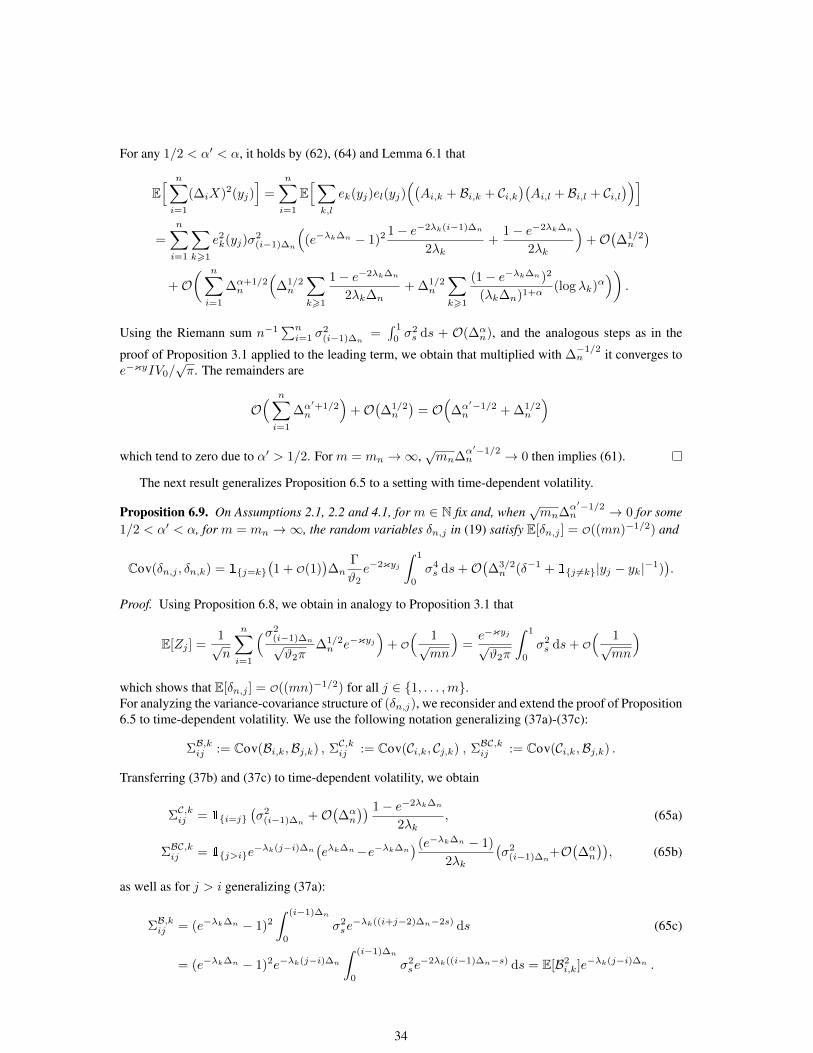
For any 1/2 < α′ < α, it holds by (62), (64) and Lemma 6.1 that

E[ n∑i=1

(∆iX)2(yj)]

=

n∑i=1

E[∑k,l

ek(yj)el(yj)((Ai,k + Bi,k + Ci,k

)(Ai,l + Bi,l + Ci,l

))]=

n∑i=1

∑k>1

e2k(yj)σ

2(i−1)∆n

((e−λk∆n − 1)2 1− e−2λk(i−1)∆n

2λk+

1− e−2λk∆n

2λk

)+O

(∆1/2n

)+O

( n∑i=1

∆α+1/2n

(∆1/2n

∑k>1

1− e−2λk∆n

2λk∆n+ ∆1/2

n

∑k>1

(1− e−λk∆n)2

(λk∆n)1+α(log λk)α

)).

Using the Riemann sum n−1∑ni=1 σ

2(i−1)∆n

=∫ 1

0σ2s ds + O(∆α

n), and the analogous steps as in the

proof of Proposition 3.1 applied to the leading term, we obtain that multiplied with ∆−1/2n it converges to

e−κyIV0/√π. The remainders are

O( n∑i=1

∆α′+1/2n

)+O

(∆1/2n

)= O

(∆α′−1/2n + ∆1/2

n

)which tend to zero due to α′ > 1/2. For m = mn →∞,

√mn∆

α′−1/2n → 0 then implies (61).

The next result generalizes Proposition 6.5 to a setting with time-dependent volatility.

Proposition 6.9. On Assumptions 2.1, 2.2 and 4.1, for m ∈ N fix and, when√mn∆

α′−1/2n → 0 for some

1/2 < α′ < α, for m = mn →∞, the random variables δn,j in (19) satisfy E[δn,j ] = O((mn)−1/2) and

Cov(δn,j , δn,k) = 1{j=k}(1 + O(1)

)∆n

Γ

ϑ2e−2κyj

∫ 1

0

σ4s ds+O

(∆3/2n (δ−1 + 1{j 6=k}|yj − yk|−1)

).

Proof. Using Proposition 6.8, we obtain in analogy to Proposition 3.1 that

E[Zj ] =1√n

n∑i=1

(σ2(i−1)∆n√ϑ2π

∆1/2n e−κyj

)+ O

( 1√mn

)=e−κyj√ϑ2π

∫ 1

0

σ2s ds+ O

( 1√mn

)which shows that E[δn,j ] = O((mn)−1/2) for all j ∈ {1, . . . ,m}.For analyzing the variance-covariance structure of (δn,j), we reconsider and extend the proof of Proposition6.5 to time-dependent volatility. We use the following notation generalizing (37a)-(37c):

ΣB,kij := Cov(Bi,k,Bj,k) , ΣC,kij := Cov(Ci,k, Cj,k) , ΣBC,kij := Cov(Ci,k,Bj,k) .

Transferring (37b) and (37c) to time-dependent volatility, we obtain

ΣC,kij = 1{i=j}(σ2

(i−1)∆n+O

(∆αn

)) 1− e−2λk∆n

2λk, (65a)

ΣBC,kij = 1{j>i}e−λk(j−i)∆n

(eλk∆n−e−λk∆n

) (e−λk∆n − 1)

2λk

(σ2

(i−1)∆n+O

(∆αn

)), (65b)

as well as for j > i generalizing (37a):

ΣB,kij = (e−λk∆n − 1)2

∫ (i−1)∆n

0

σ2se−λk((i+j−2)∆n−2s) ds (65c)

= (e−λk∆n − 1)2e−λk(j−i)∆n

∫ (i−1)∆n

0

σ2se−2λk((i−1)∆n−s) ds = E[B2

i,k]e−λk(j−i)∆n .

34

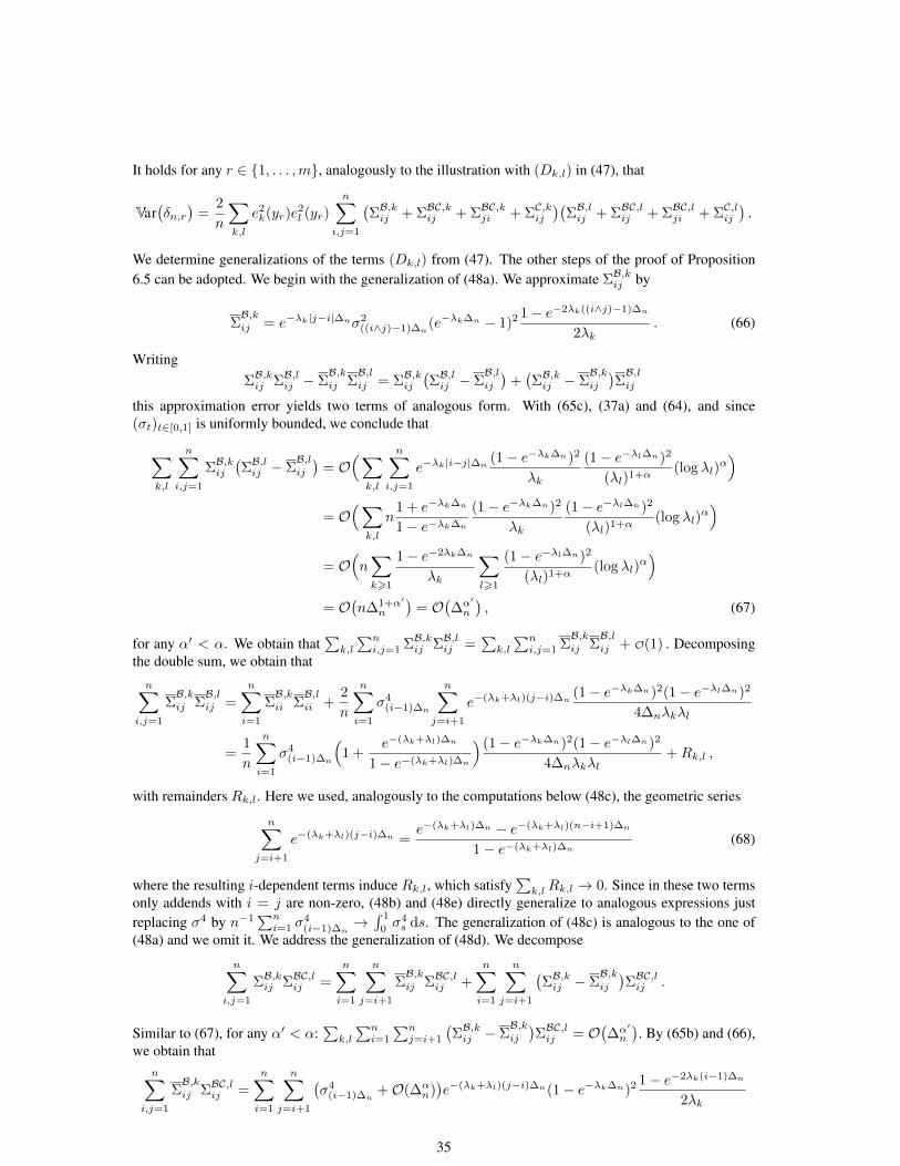
It holds for any r ∈ {1, . . . ,m}, analogously to the illustration with (Dk,l) in (47), that

Var(δn,r

)=

2

n

∑k,l

e2k(yr)e

2l (yr)

n∑i,j=1

(ΣB,kij + ΣBC,kij + ΣBC,kji + ΣC,kij

)(ΣB,lij + ΣBC,lij + ΣBC,lji + ΣC,lij

).

We determine generalizations of the terms (Dk,l) from (47). The other steps of the proof of Proposition6.5 can be adopted. We begin with the generalization of (48a). We approximate ΣB,kij by

ΣB,kij = e−λk|j−i|∆nσ2

((i∧j)−1)∆n(e−λk∆n − 1)2 1− e−2λk((i∧j)−1)∆n

2λk. (66)

WritingΣB,kij ΣB,lij − Σ

B,kij Σ

B,lij = ΣB,kij

(ΣB,lij − Σ

B,lij

)+(ΣB,kij − Σ

B,kij

)ΣB,lij

this approximation error yields two terms of analogous form. With (65c), (37a) and (64), and since(σt)t∈[0,1] is uniformly bounded, we conclude that

∑k,l

n∑i,j=1

ΣB,kij(ΣB,lij − Σ

B,lij

)= O

(∑k,l

n∑i,j=1

e−λk|i−j|∆n(1− e−λk∆n)2

λk

(1− e−λl∆n)2

(λl)1+α(log λl)

α)

= O(∑k,l

n1 + e−λk∆n

1− e−λk∆n

(1− e−λk∆n)2

λk

(1− e−λl∆n)2

(λl)1+α(log λl)

α)

= O(n∑k>1

1− e−2λk∆n

λk

∑l>1

(1− e−λl∆n)2

(λl)1+α(log λl)

α)

= O(n∆1+α′

n

)= O

(∆α′

n

), (67)

for any α′ < α. We obtain that∑k,l

∑ni,j=1 ΣB,kij ΣB,lij =

∑k,l

∑ni,j=1 Σ

B,kij Σ

B,lij + O(1) . Decomposing

the double sum, we obtain that

n∑i,j=1

ΣB,kij Σ

B,lij =

n∑i=1

ΣB,kii Σ

B,lii +

2

n

n∑i=1

σ4(i−1)∆n

n∑j=i+1

e−(λk+λl)(j−i)∆n(1− e−λk∆n)2(1− e−λl∆n)2

4∆nλkλl

=1

n

n∑i=1

σ4(i−1)∆n

(1 +

e−(λk+λl)∆n

1− e−(λk+λl)∆n

) (1− e−λk∆n)2(1− e−λl∆n)2

4∆nλkλl+Rk,l ,

with remainders Rk,l. Here we used, analogously to the computations below (48c), the geometric series

n∑j=i+1

e−(λk+λl)(j−i)∆n =e−(λk+λl)∆n − e−(λk+λl)(n−i+1)∆n

1− e−(λk+λl)∆n(68)

where the resulting i-dependent terms induce Rk,l, which satisfy∑k,lRk,l → 0. Since in these two terms

only addends with i = j are non-zero, (48b) and (48e) directly generalize to analogous expressions justreplacing σ4 by n−1

∑ni=1 σ

4(i−1)∆n

→∫ 1

0σ4s ds. The generalization of (48c) is analogous to the one of

(48a) and we omit it. We address the generalization of (48d). We decompose

n∑i,j=1

ΣB,kij ΣBC,lij =

n∑i=1

n∑j=i+1

ΣB,kij ΣBC,lij +

n∑i=1

n∑j=i+1

(ΣB,kij − Σ

B,kij

)ΣBC,lij .

Similar to (67), for any α′ < α:∑k,l

∑ni=1

∑nj=i+1

(ΣB,kij − Σ

B,kij

)ΣBC,lij = O

(∆α′

n

). By (65b) and (66),

we obtain thatn∑

i,j=1

ΣB,kij ΣBC,lij =

n∑i=1

n∑j=i+1

(σ4

(i−1)∆n+O(∆α

n))e−(λk+λl)(j−i)∆n(1− e−λk∆n)2 1− e−2λk(i−1)∆n

2λk

35

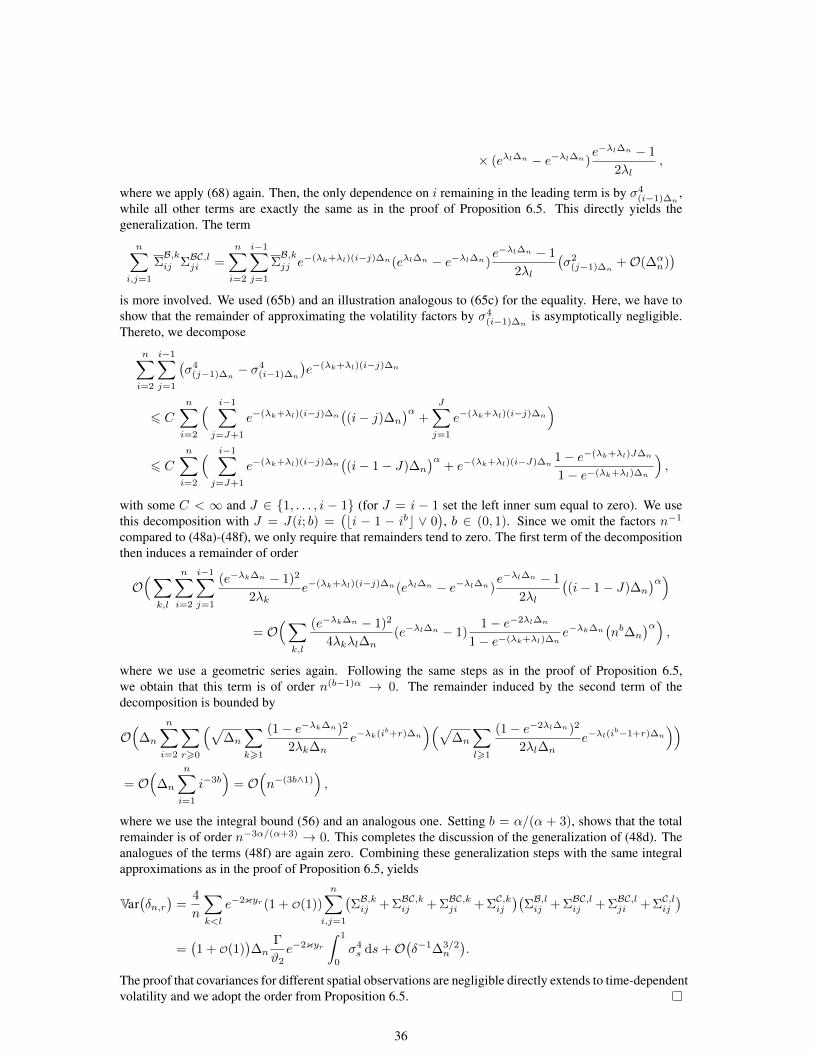
× (eλl∆n − e−λl∆n)e−λl∆n − 1

2λl,

where we apply (68) again. Then, the only dependence on i remaining in the leading term is by σ4(i−1)∆n

,while all other terms are exactly the same as in the proof of Proposition 6.5. This directly yields thegeneralization. The term

n∑i,j=1

ΣB,kij ΣBC,lji =

n∑i=2

i−1∑j=1

ΣB,kjj e

−(λk+λl)(i−j)∆n(eλl∆n − e−λl∆n)e−λl∆n − 1

2λl

(σ2

(j−1)∆n+O(∆α

n))

is more involved. We used (65b) and an illustration analogous to (65c) for the equality. Here, we have toshow that the remainder of approximating the volatility factors by σ4

(i−1)∆nis asymptotically negligible.

Thereto, we decompose

n∑i=2

i−1∑j=1

(σ4

(j−1)∆n− σ4

(i−1)∆n

)e−(λk+λl)(i−j)∆n

6 C

n∑i=2

( i−1∑j=J+1

e−(λk+λl)(i−j)∆n((i− j)∆n

)α+

J∑j=1

e−(λk+λl)(i−j)∆n

)

6 C

n∑i=2

( i−1∑j=J+1

e−(λk+λl)(i−j)∆n((i− 1− J)∆n

)α+ e−(λk+λl)(i−J)∆n

1− e−(λk+λl)J∆n

1− e−(λk+λl)∆n

),

with some C < ∞ and J ∈ {1, . . . , i − 1} (for J = i − 1 set the left inner sum equal to zero). We usethis decomposition with J = J(i; b) =

(bi − 1 − ibc ∨ 0

), b ∈ (0, 1). Since we omit the factors n−1

compared to (48a)-(48f), we only require that remainders tend to zero. The first term of the decompositionthen induces a remainder of order

O(∑k,l

n∑i=2

i−1∑j=1

(e−λk∆n − 1)2

2λke−(λk+λl)(i−j)∆n(eλl∆n − e−λl∆n)

e−λl∆n − 1

2λl

((i− 1− J)∆n

)α)= O

(∑k,l

(e−λk∆n − 1)2

4λkλl∆n(e−λl∆n − 1)

1− e−2λl∆n

1− e−(λk+λl)∆ne−λk∆n

(nb∆n

)α),

where we use a geometric series again. Following the same steps as in the proof of Proposition 6.5,we obtain that this term is of order n(b−1)α → 0. The remainder induced by the second term of thedecomposition is bounded by

O(

∆n

n∑i=2

∑r>0

(√∆n

∑k>1

(1− e−λk∆n)2

2λk∆ne−λk(ib+r)∆n

)(√∆n

∑l>1

(1− e−2λl∆n)2

2λl∆ne−λl(i

b−1+r)∆n

))= O

(∆n

n∑i=1

i−3b)

= O(n−(3b∧1)

),

where we use the integral bound (56) and an analogous one. Setting b = α/(α + 3), shows that the totalremainder is of order n−3α/(α+3) → 0. This completes the discussion of the generalization of (48d). Theanalogues of the terms (48f) are again zero. Combining these generalization steps with the same integralapproximations as in the proof of Proposition 6.5, yields

Var(δn,r

)=

4

n

∑k<l

e−2κyr (1 + O(1))

n∑i,j=1

(ΣB,kij + ΣBC,kij + ΣBC,kji + ΣC,kij

)(ΣB,lij + ΣBC,lij + ΣBC,lji + ΣC,lij

)=(1 + O(1)

)∆n

Γ

ϑ2e−2κyr

∫ 1

0

σ4s ds+O

(δ−1∆3/2

n

).

The proof that covariances for different spatial observations are negligible directly extends to time-dependentvolatility and we adopt the order from Proposition 6.5.

36

Based on the two previous propositions, we now prove Theorem 4.2. The M-estimator is associated tothe contrast function, with η := (IV0,κ),

K(η, η′) :=

∫ 1−δ

δ

(fη(y)− fη′(y)

)2dy .

Step 1: We prove for Kn(η′) := 1m

∑mj=1(Zj − fη′(yj))2 that

Kn(η′)−K(η, η′)Pη−→ 0.

To verify this convergence in probability, we decompose

Kn(η′) =1

m

m∑j=1

(fη(yj)− fη′(yj)

)2 − 2

m

m∑j=1

δn,j(fη(yj)− fη′(yj)

)+

1

m

m∑j=1

δ2n,j . (69)

The first term converges to∫ 1−δδ

(fη(y) − fη′(y)

)2dy as m → ∞. For the second term we have with

g := fη − fη′ , being uniformly bounded on Ξ× [0, 1], by Proposition 6.9

Pη(∣∣∣ 2

m

m∑j=1

δn,jg(yj)∣∣∣ > ε

)6 ε−2 4

m2

m∑j,k=1

|E[δn,jδn,k]| · |g(yj)g(yk)|

6 ε−2 4

m2

m∑j,k=1

(|Cov(δn,j , δn,k)|+ |E[δn,j ]E[δn,k]|

)· |g(yj)g(yk)|

= O( 4

m2

m∑j,k=1

(1{j=k}∆n

Γ

ϑ2e−2κyj

∫ 1

0

σ4s ds+ ∆3/2

n

(δ−1 + 1{j 6=k}|yj − yk|−1

)+ (mn)−1

))= O

(∆n/m

).

For the third term in (69) we obtain with E[δ2n,j ] = ∆nΓe−2κyj

∫ 1

0σ4s ds/ϑ2(1 + O(1)):

Pη( 1

m

m∑j=1

δ2n,j > ε

)6 m sup

jPη(δ2n,j > ε/2

)6

2m

εsupj

E[δ2n,j

]= O(m∆n) .

Step 2: We prove consistency of η = (IV0, κ). Since K(η, ·) and Kn are continuous, consistencyfollows from continuous mapping if the stochastic convergence of Kn is also uniform. Now, tightnessfollows from the equicontinuity:

limδ→0

lim supn→∞

Pη(

sup|η′−η|<δ

|Kn(η)−Kn(η′)| > ε)

6 limδ→0

lim supn→∞

1

εE[

sup|η′−η|<δ

|Kn(η)−Kn(η′)|]

= limδ→0

lim supn→∞

1

εE[

sup|η′−η|<δ

∣∣∣ 1

m

m∑j=1

(2Zj(fη(yj)− fη′(yj)) + f2

η′(yj)− f2η (yj)

)∣∣∣].The last line converges to zero by dominated convergence and uniform continuity of fη in η.

Step 3: To prove the central limit theorem, we follow the classical theory elaborated in (Dacunha-Castelle and Duflo, 1986, Chapter 3.3.4). We calculate the first and second derivative of Kn(η). Thegradient and the Hessian matrix are given by

Kn(η) = − 2

m

m∑j=1

(Zj − fη(yj))e−κyj√

π

(1

−IV0 yj

),

37

Kn(η) =2

m

m∑j=1

(Zj − fη(yj)

)e−κyj√π

(0 yjyj −IV0 y

2j

)+

2

m

m∑j=1

e−2κyj

π

(1 −IV0 yj

−IV0 yj IV 20 y

2j

),

respectively. The mean value theorem yields on an event with probability converging to one that

0 = Kn(η) = Kn(η) + Kn(η∗)(η − η)

for some η∗ between η and η and thus η − η = −Kn(η∗)−1Kn(η), on the event where η is close to η andwhere Kn(η∗) is invertible.

To show a central limit theorem for Kn(η), we set

χn,i := − 2√m

m∑j=1

((∆iX)2(yj)−

√∆nfη(yj)

)e−κyj√π

(1

−IV0 yj

),

such that√nmKn(η) =

∑ni=1 χn,i. Using Proposition 6.9, the variance-covariance matrix of

∑ni=1 χn,i

can be calculated as follows:

COV( n∑i=1

χn,i

)=

4

m

m∑j,k=1

e−κ(yj+yk)

πCov

( n∑i=1

(∆iX)2(yj),

n∑i=1

(∆iX)2(yk))( 1 −IV0 yk−IV0 yj IV 2

0 yjyk

)

=4n2∆n

m

m∑j,k=1

e−2κ(yj+yk)

πCov

(Vn(yj), Vn(yk)

)( 1 −IV0 yk−IV0 yj IV 2

0 yjyk

)

=4

m

m∑j,k=1

e−2κ(yj+yk)

π

(1{j=k}

Γ

ϑ2

∫ 1

0

σ4s ds+O

(∆1/2n

1{j 6=k}

|yj − yk| ∧ δ

))( 1 −IV0 yk−IV0 yj IV 2

0 yjyk

)

=4 Γ∫ 1

0σ4s ds

ϑ2π

( 1m

∑j e−4κyj −IV0

1m

∑j yje

−4κyj

−IV01m

∑j yje

−4κyj IV 20

1m

∑j y

2j e−4κyj

)(1 +O(∆1/2

n (logm)m)).

If m→∞, then the matrix in the last display converges on Assumption 2.1, when y1 = δ and ym = 1− δ,to U(η) from (22). In particular, Jensen’s inequality shows that the covariance matrix is positive definitefor sufficiently large m. We will apply again Utev’s central limit theorem together with the Cramer-Wolddevice to deduce the two-dimensional central limit theorem. Analogously to ζn,i from (41) in the proof ofTheorem 3.4, the triangular array (χn,i) and any linear combination of its components satisfy the mixing-type Condition (58d) based on a direct modification of Corollary 6.7. By the above considerations for thevariance, (χn,i) and any linear combination of its components satisfy Conditions (58a) and (58b). TheLyapunov condition and hence (58c) follows from

E[|χn,i|4] = O(m2 max

jE[(∆iX(yj))

8])

= O(m2∆2n) = O(1) ,

similar to (60). Therefore, we have under Pη for n → ∞ and m = mn → ∞, when√mn∆

α′−1/2n → 0

for some α′ < α, that√mnKn(η)

d→ N(

0,4 Γ∫ 1

0σ4s ds

ϑ2πU(η)

).

As the final step, we will verify Pη-convergence in probability of Kn(ηn) to a deterministic, invertible

matrix for any sequence ηnPη→ η. Since for any such sequence, Zj−fηn(yj) = fη(yj)−fηn(yj)+δn,j

Pη→ 0

holds under Pη by continuity of fη in the parameter and owing to δn,jPη→ 0, we indeed have

Kn(ηn) =2

m

m∑j=1

e−2κyj

π

(1 −IV0 yj

−IV0 yj IV 20 y

2j

)+ OPη (1)

Pη→ 2

πV (η) ,

with V (η) from (23) using that y1 = δ and ym = 1 − δ. Jensen’s inequality verifies that V (η) is strictlypositive definite. We obtain the limit distribution in (21).

38

6.4. Proof of Corollary 4.3

For the statistics analogous to (39), the bias is asymptotically negligible by Proposition 6.8. For thecentered versions, we obtain Conditions (58a) and (58b) with the asymptotic variance in (25) from Proposi-tion 6.9. Since (σ2

t )06t61 is uniformly bounded, the proofs of the Lyapunov condition and the mixing-typeconditions from Proposition 6.6 and Corollary 6.7 readily extend to the time-varying setting. With Peligradand Utev (1997, Thm. B), we thus conclude (24) and (25). A simple generalization shows consistency ofthe integrated quarticity estimator and thus (26).

Acknowledgements

The authors are grateful to two anonymous referees whose valuable comments helped improving thepaper. We also thank Jan Kallsen and Mathias Vetter for helpful comments. Mathias Trabs gratefullyacknowledges financial support by the DFG research fellowship TR 1349/1-1.

References

Bagchi, A. and Kumar, K. S. (2001). An infinite factor model for the interest rate derivatives. In Kohlmann,M. and Tang, S., editors, Mathematical Finance: Workshop of the Mathematical Finance ResearchProject, Konstanz, Germany, October 5–7, 2000, pages 59–68. Birkhauser Basel, Basel.

Barndorff-Nielsen, O. E., Corcuera, J. M., and Podolskij, M. (2009). Power variation for gaussian processeswith stationary increments. Stochastic Processes and their Applications, 119(6):1845 – 1865.

Bishwal, J. P. N. (2002). The Bernstein-von Mises theorem and spectral asymptotics of Bayes estimatorsfor parabolic SPDEs. Journal of the Australian Mathematical Society, 72(2):287–298.

Bouchaud, J.-P., Sagna, N., Cont, R., El-Karoui, N., and Potters, M. (1999). Phenomenology of the interestrate curve. Applied Mathematical Finance, 6(3):209–232.

Chong, C. (2018). High-frequency analysis of parabolic stochastic pdes. arXiv:1806.06959.

Cialenco, I. (2018). Statistical inference for spdes: an overview. Statistical Inference for Stochastic Pro-cesses, 21(2):309–329.

Cialenco, I. and Glatt-Holtz, N. (2011). Parameter estimation for the stochastically perturbed Navier-Stokesequations. Stochastic Processes and their Applications, 121(4):701–724.

Cialenco, I., Gong, R., and Huang, Y. (2018). Trajectory fitting estimators for spdes driven by additivenoise. Statistical Inference for Stochastic Processes, 21(1):1–19.

Cialenco, I. and Huang, Y. (2019). A note on parameter estimation for discretely sampled spdes. Stochasticsand Dynamics, forthcoming, doi: 10.1142/S0219493720500161.

Cont, R. (2005). Modeling term structure dynamics: an infinite dimensional approach. InternationalJournal of Theoretical and Applied Finance, 8(3):357–380.

Da Prato, G. and Zabczyk, J. (1992). Stochastic equations in infinite dimensions, volume 44 of Encyclope-dia of Mathematics and its Applications. Cambridge University Press, Cambridge.

Dacunha-Castelle, D. and Duflo, M. (1986). Probability and statistics. Vol. II. Springer-Verlag, New York.Translated from the French by David McHale.

Fox, J. and Weisberg, S. (2000). Nonlinear regression and nonlinear least squares in r. An Appendix to An RCompanion to Applied Regression, second edition, https://socserv.socsci.mcmaster.ca/jfox/Books/Companion/appendix/Appendix-Nonlinear-Regression.pdf.

Hairer, M. (2013). Solving the KPZ equation. Annals of Mathematics, 178(2):559–664.

39

Heath, D., Jarrow, R., and Morton, A. (1992). Bond pricing and the term structure of interest rates: a newmethodology for contingent claims valuation. Econometrica, 60(1):77–105.

Hubner, M., Khasminskii, R., and Rozovskii, B. L. (1993). Two examples of parameter estimation forstochastic partial differential equations. In Stochastic processes, pages 149–160. Springer, New York.

Hubner, M. and Lototsky, S. (2000). Asymptotic analysis of a kernel estimator for parabolic SPDE’s withtime-dependent coefficients. The Annals of Applied Probability, 10(4):1246–1258.

Hubner, M. and Rozovskiı, B. L. (1995). On asymptotic properties of maximum likelihood estimators forparabolic stochastic PDE’s. Probability Theory and Related Fields, 103(2):143–163.

Jacod, J. (1997). On continuous conditional gaussian martingales and stable convergence in law. Seminairede Probabilities, pages 232–246.

Jacod, J. and Protter, P. (2012). Discretization of processes. Springer.

Kolmogorov, A. and Rozanov, Y. (1961). On strong mixing conditions for stationary Gaussian processes.Theory of Probability and its Applications, 5:204–208.

Lototsky, S. V. (2009). Statistical inference for stochastic parabolic equations: a spectral approach. Publi-cacions Matematiques, 53(1):3–45.

Markussen, B. (2003). Likelihood inference for a discretely observed stochastic partial differential equa-tion. Bernoulli, 9(5):745–762.

Mohapl, J. (1997). On estimation in the planar Ornstein-Uhlenbeck process. Communications in Statistics.Stochastic Models, 13(3):435–455.

Musiela, M. (1993). Stochastic pdes and term structure models. Journees Internationales de Finance,IGR-AFFI, La Baule.

Mykland, P. and Zhang, L. (2009). Inference for continuous semimartingales observed at high frequency.Econometrica, 77(5):1403–1445.

Peligrad, M. and Utev, S. (1997). Central limit theorem for linear processes. The Annals of Probability,25(1):443–456.

Prakasa Rao, B. L. S. (2002). Nonparametric inference for a class of stochastic partial differential equationsbased on discrete observations. Sankhya Ser. A, 64(1):1–15.

Santa Clara, P. and Sornette, D. (2001). The dynamics of the forward interest rate curve with stochasticstring shocks. Review of Financial Studies, 14(1):149 – 185.

Schmidt, T. (2006). An infinite factor model for credit risk. International Journal of Theoretical andApplied Finance, 9(1):43–68.

Swanson, J. (2007). Variations of the solution to a stochastic heat equation. The Annals of Probability,35(6):2122–2159.

Tuckwell, H. C. (2013). Stochastic partial differential equations in neurobiology: Linear and nonlinearmodels for spiking neurons. In Stochastic Biomathematical Models, pages 149–173. Springer.

Utev, S. A. (1990). Central limit theorem for dependent random variables. In Probability theory andmathematical statistics, Vol. II (Vilnius, 1989), pages 519–528. “Mokslas”, Vilnius.

Walsh, J. B. (1986). An introduction to stochastic partial differential equations. Springer.

Winkelmann, L., Bibinger, M., and Linzert, T. (2016). Ecb monetary policy surprises: Identificationthrough cojumps in interest rates. Journal of Applied Econometrics, 31(4):613–629.

40