Visualizing the Phase-Space Dynamics of an External Cavity

Semiconductor Laser

C. Y. Chang,1, 2, ∗ Michael J. Wishon,2, 3 Daeyoung Choi,2, 3 K. Merghem,4 Abderrahim

Ramdane,4 Francois Lelarge,4, † A. Martinez,4 A. Locquet,2, 3 and D. S. Citrin2, 3, ‡

1Georgia Institute of Technology, School of Physics, Atlanta, Georgia 30332-0250 USA

2UMI 2958 Georgia Tech-CNRS, Georgia Tech Lorraine,

2 Rue Marconi F-57070, Metz, France

3School of Electrical and Computer Engineering,

Georgia Institute of Technology, Atlanta, Georgia 30332-0250 USA

4Center for Nanosciences and Nanotechnologies (CNRS-C2N),

Route de Nozay, 91460 Marcoussis-France

(Dated: September 21, 2017)

Abstract

We map the phase-space trajectories of an external-cavity semiconductor laser using phase por-

traits. This is both a visualization tool as well as a thoroughly quantitative approach enabling

unprecedented insight into the dynamical regimes, from continuous-wave through coherence col-

lapse as feedback is increased. Namely, the phase portraits in the intensity versus laser-diode

terminal-voltage (serving as a surrogate for inversion) plane are mapped out. We observe a route

to chaos interrupted by two types of limit cycles, a subharmonic regime and period-doubled dy-

namics at the edge of chaos. The transition of the dynamics are analyzed utilizing bifurcation

diagrams for both the optical intensity and the laser-diode terminal voltage. These observations

provide visual insight into the dynamics in these systems.

1

arX

iv:1

709.

0679

5v1

[nl

in.C

D]

20

Sep

2017

INTRODUCTION

The complex dynamics experienced by a nonlinear system for given initial conditions

corresponds to a trajectory in phase space that span all the system’s dynamical variables.

Visualizing the phase-space dynamics both provides a heuristic tool as well as opens a

quantitative window onto the dynamics that may otherwise be difficult to apprehend. For

a laser diode (LD) with time-delayed optical feedback, otherwise known as an external-

cavity semiconductor laser (ECL), a three dimensional projection is typically used. This

projection is spanned by the optical intensityI∝|E|2 (with E the slowly-varying amplitude

of the optical field), the optical phase φ, and the inversion n in the gain medium. The

high speed and high dynamical dimensionality of ECLs has attracted broad interest for

various applications, ranging from radar [3], ultrafast random bit generation [4, 5], and

optoelectronic oscillators [6, 7], to name a few. Moreover, the intrinsic dynamics of ECLs

have attracted attention to implement a number of information-processing functionalities

in the physical layer, including chaotic encrypted data communications [8–10], compressive

sensing [11], and reservoir computing [13, 14]. But to realize the full potential of such

applications, a detailed knowledge of the complex dynamics of ECLs is required [15], and

despite 50 years of study, there are basic issues that remain to be elucidated. In Ref. [12],

phase plots of the optical intensity, phase, and laser voltage were obtained but only for

the complex chaotic regime of low-frequency fluctuations. In this paper, we focus on phase

portraits revealing the first instabilities that lead the ECL into a chaotic regime.

It has been pointed out, based on delay embedding theory, that the phase portrait in

|E| and n can be reconstructed by plotting |E(t)| versus |E(t− τ)| parametrically in time.

Refs. [16] and [17] investigate the requirements for accessing this information by recon-

structing from the signal and delayed signal in other deterministic time-delayed systems.

Theoretically, the reconstructed phase portraits and the experimental phase portraits may

share some (invariant) properties; however, they are limited to the vicinity of an attractor

along with other mathematical conditions discussed in Ref. [18]. Note, however, it is not

a foregone conclusion that such reconstructed phase portraits are necessarily correct, even

proximate to an attractor. Clearly, the ability to obtain experimental phase portraits takes

precedence over any reconstructed phase portraits. Our work opens the way for such a de-

tailed comparison, though the aim of the present work is to introduce the technique rather

2

than to provide such a comparison.

From a more general perspective, ECLs provide time-delayed feedback systems in which

a number of key parameters can be controlled, and combining this with their relative ease of

implementation on the tabletop or within photonics integrated circuits, these systems serve

as excellent test-beds for the bifurcation analysis for high-dimensional nonlinear systems

[19, 20]. The dynamics of ECLs are commonly described by the Lang-Kobayashi (LK)

model [21]. The LK model provides a coupled delay-differential-equation description of

the system variables, viz. E, n, and φ. By adjusting various control parameters (feedback

strength η, external-cavity length L=c/(2τ) with τ the feedback time, injection current J),

various dynamical regimes can be accessed [22–25].

The LK model allows one to explore dynamical trends as various parameters are tuned;

most studies focus on η [27–30] and visualize these trends by means of bifurcation diagrams

(BD). Recently, we demonstrated experimental BDs for the optical intensity I(t) as η is

varied [22, 31, 32]. Both theoretical and experimental BDs provide global perspectives on

the evolution of the dynamical regimes as the chosen parameter is varied; in particular, one

can test predictions of the sequence of bifurcations based on the LK model. Most studies

to date, however, only focus on I(t)∝E2(t) [33]. To more thoroughly map the dynamics

in phase space, it is necessary to probe additional dynamical degrees of freedom. Changes

in n in the gain region can be obtained from the LD terminal voltage V (t) at fixed J [35–

37]. We recently reported such measurement [38], while varying the control parameter η,

in Refs. [6, 7]. This allowed us to plot BDs based on V (t). These investigations provide

another component of a global perspective of the route to chaos in ECLs. In Ref. [7], a

largest-Lyapunov-exponent analysis was applied to both I(t) and V (t) verifying that the

measurement of V (t) provides information of comparable dynamical complexity to that

provided by I(t). In order to interpret the information contained in this additional degree

of freedom, it is essential to focus on its dynamics compared to the better-known dynamics

in I(t). While their relationship has been studied theoretically [12, 15, 20, 39] in various

dynamical regimes, to date experimental verification, outside of LFF, is absent.

In this study, we present simultaneous measurements of the time series (TS) I(t) and

V (t) on the route to chaos, from continuous-wave (CW) to coherence collapse (CC). The

TSs, when plotted parametrically in time t in the I-V plane (V serving as a surrogate for

n) provide a phase portrait of the dynamics, i.e., the resulting plot is a projection in the φ

3

direction of the phase-space trajectory onto the I-V plane, where φ is the phase difference

between the input and output electric fields. While numerous theoretical studies of phase

portraits in ECLs based on the LK model have been presented in the literature, e.g., [15, 40],

to our knowledge, the experimental phase portraits presented here are the first published

mapping out the route to chaos in an ECL. Together with the global view provided by the

BDs [5, 6, 30–32], the phase portraits provide unprecedented detailed insight into the phase-

space dynamics in various regimes and open the way to more thorough testing of theoretical

predictions.

Before embarking on our more detailed discussion, it is helpful to orient ourselves by

means of simple examples. To start, consider an ECL under CW operation, for which

I(t) and V (t) are constant. In this case, a parametric plot of I(t) and V (t) in t will be a

point in the I-V plane. Now consider relaxation oscillations (RO), a small-signals model

accounting for the dynamics of I(t) and n(t) given a small temporal perturbation shows

that I(t) and n(t) both exhibit damped sinusoidal oscillations near the LD RO frequency

fRO with n(t) lagging I(t) by π/2 [42]. In an ECL, for certain ranges of η, these ROs may

become undamped and shifted in frequency [43–48]. Consequently, a parametric plot of I(t)

and V (t) in t, again the corresponding phase portrait, will be an ellipse with semi-major

axis with negative slope in the I-V plane. Of course, in other dynamical regimes, the phase

portrait will reflect the more complex combined dynamics of I(t) and V (t), as we see below.

EXPERIMENTAL SETUP

A schematic of our ECL setup is shown in Fig. 1. For our experiments, we employ a single

longitudinal-mode edge-emitting InGaAsP distributed feedback (DFB) LD containing seven

quantum wells in the active region [6]. The grating is designed and fabricated to achieve a

k product of 50 cm−1 and the length l of the LD cavity is 600 µm, achieving a kl value of

3. The LD is that of Ref. [41]. The LD emits at 1550 nm with a free-running threshold

current Jth=29.8 mA. We simultaneously measure I(t) and V (t) where we synchronize the

two via cross-correlation of two signals as the optical path length is varied; the signals are

synchronized to within 1 ps, which is much shorter than any relevant dynamical timescale.

During the experiment, the OSA continuously measures the optical spectrum for each

η. V (t) is measured across the LD injection terminals utilizing a radio-frequency (RF)

4

P

QWP

Mirror

L

OSC - 12 GHz

VAC(t)IAC(t)

DFBLaser

Bias Network

AMP - 30 dB

Multimeter

CurrentSource

BS

BS

Isolator

Eηi(ω)OSA

VDC(ηi)

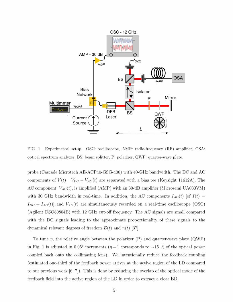
FIG. 1. Experimental setup. OSC: oscilloscope, AMP: radio-frequency (RF) amplifier, OSA:

optical spectrum analyzer, BS: beam splitter, P: polarizer, QWP: quarter-wave plate.

probe (Cascade Microtech AE-ACP40-GSG-400) with 40-GHz bandwidth. The DC and AC

components of V (t) =VDC + VAC(t) are separated with a bias tee (Keysight 11612A). The

AC component, VAC(t), is amplified (AMP) with an 30-dB amplifier (Microsemi UA030VM)

with 30 GHz bandwidth in real-time. In addition, the AC components IAC(t) [of I(t) =

IDC + IAC(t)] and VAC(t) are simultaneously recorded on a real-time oscilloscope (OSC)

(Agilent DSO80804B) with 12 GHz cut-off frequency. The AC signals are small compared

with the DC signals leading to the approximate proportionality of these signals to the

dynamical relevant degrees of freedom E(t) and n(t) [37].

To tune η, the relative angle between the polarizer (P) and quarter-wave plate (QWP)

in Fig. 1 is adjusted in 0.05◦ increments (η= 1 corresponds to ∼15 % of the optical power

coupled back onto the collimating lens). We intentionally reduce the feedback coupling

(estimated one-third of the feedback power arrives at the active region of the LD compared

to our previous work [6, 7]). This is done by reducing the overlap of the optical mode of the

feedback field into the active region of the LD in order to extract a clear BD.

5

RESULTS AND DISCUSSION

As we increase η, E(t) and E(t−τ) interact within the nonlinear active region of the LD,

giving rise to the various types of dynamics discussed below. These dynamics are manifested

in both n(t) [measured through V (t)] and E(t) [measured through I(t)]. The TSs at the

various values of η can be used to plot the BDs shown in this section. We start with a global

picture of the route to chaos presented in terms of BDs for I(t) and V (t) as η is increased. In

the subsections below, we consider phase portraits within various dynamical regimes along

the route to chaos.

Figure 2 shows the BD obtained from (a) V (t) and (b) I(t) as a function of η. Each BD

is obtained by plotting the density of local extrema of the corresponding TS as a function

of η. The density is high in white, intermediate in shades of orange, but low in black.

The value reflects the turning point of the trajectories (maxima and minima in both V

and I), and thus for a given η, regions showing small ranges of pronounced high- and low-

density contrast tend to represent dynamical regimes exhibiting repetitive (more stable)

trajectories. The region for η > 0.64 in Fig. 2(b), however, does not correspond to a small

number of maximum/minimum values of I(t), but to chaotic behavior. [Note that the BD

for V (t) in Fig. 2(a) shows less clear features due to additional noise and filtering in the

voltage measurement; nonetheless, as noted above we have confirmed that V (t) contains

dynamical complexity comparable to that of I(t) indicating that any filtering of V (t) retains

information on crucial information-theroretic timescales.] In Fig. 2(b) the dynamical regime

is labelled with the abbreviation of each regime [32]; see Table I for the ranges of η and their

correspondence to dynamical regime.

The system evolution can be interpreted as trajectories in phase space in the vicinity of

external-cavity modes (ECMs) that are the stable steady-state solutions of the LK equations;

the unstable solutions are known as antimodes [21]. Each ECM is associated with a different

standing-wave solution in the external cavity, and thus the various ECMs are separated in

frequency approximately by the external-cavity free-spectral range fτ =τ−1 =c/(2L) = 0.36

GHz for L = 42 cm. We can track the ECMs that participate in the dynamics for a given

η from the optical spectrum as in Fig. 2(c). The bright features in Fig. 2(c) at each η

show the active ECMs. For example, we can identify the dominant ECM in the periodic

regime (0.29≤ η ≤ 0.4); it is the third ECM (i.e., ECM 3) above the minimum-linewidth

6

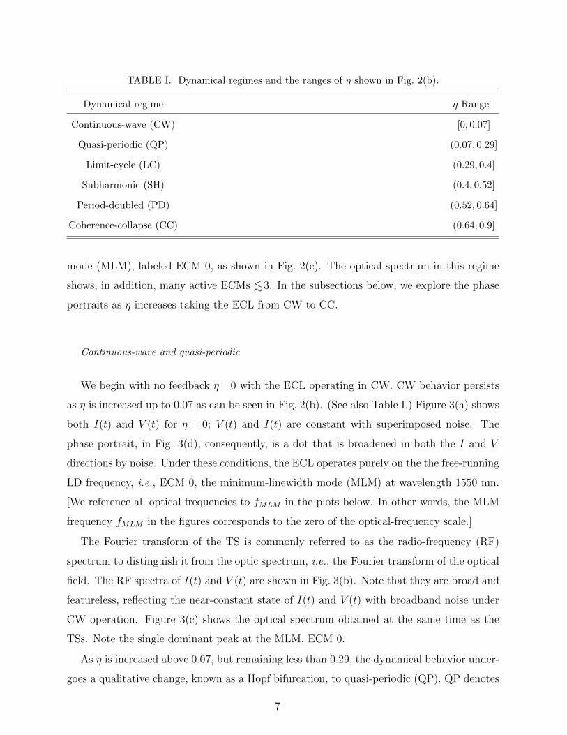
TABLE I. Dynamical regimes and the ranges of η shown in Fig. 2(b).

Dynamical regime η Range

Continuous-wave (CW) [0, 0.07]

Quasi-periodic (QP) (0.07, 0.29]

Limit-cycle (LC) (0.29, 0.4]

Subharmonic (SH) (0.4, 0.52]

Period-doubled (PD) (0.52, 0.64]

Coherence-collapse (CC) (0.64, 0.9]

mode (MLM), labeled ECM 0, as shown in Fig. 2(c). The optical spectrum in this regime

shows, in addition, many active ECMs .3. In the subsections below, we explore the phase

portraits as η increases taking the ECL from CW to CC.

Continuous-wave and quasi-periodic

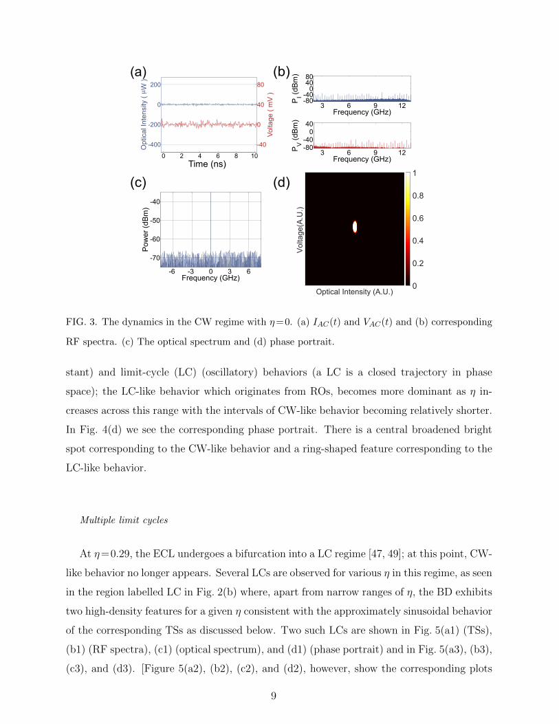
We begin with no feedback η=0 with the ECL operating in CW. CW behavior persists

as η is increased up to 0.07 as can be seen in Fig. 2(b). (See also Table I.) Figure 3(a) shows

both I(t) and V (t) for η = 0; V (t) and I(t) are constant with superimposed noise. The

phase portrait, in Fig. 3(d), consequently, is a dot that is broadened in both the I and V

directions by noise. Under these conditions, the ECL operates purely on the the free-running

LD frequency, i.e., ECM 0, the minimum-linewidth mode (MLM) at wavelength 1550 nm.

[We reference all optical frequencies to fMLM in the plots below. In other words, the MLM

frequency fMLM in the figures corresponds to the zero of the optical-frequency scale.]

The Fourier transform of the TS is commonly referred to as the radio-frequency (RF)

spectrum to distinguish it from the optic spectrum, i.e., the Fourier transform of the optical

field. The RF spectra of I(t) and V (t) are shown in Fig. 3(b). Note that they are broad and

featureless, reflecting the near-constant state of I(t) and V (t) with broadband noise under

CW operation. Figure 3(c) shows the optical spectrum obtained at the same time as the

TSs. Note the single dominant peak at the MLM, ECM 0.

As η is increased above 0.07, but remaining less than 0.29, the dynamical behavior under-

goes a qualitative change, known as a Hopf bifurcation, to quasi-periodic (QP). QP denotes

7

0.2 0.4 0.6 0.8

6

3

0

-3

-6-70

-65

-60

-55

-50

Vol

tage

(A

. U.)

(a)

(b)

(c)

Inte

nsity

(A

. U.)

CW QP LC SH PD CC

Feedback strength,η

Fre

quen

cy (

GH

z)

FIG. 2. BDs illustrating the various dynamical regimes as η is varied: (a) for V (t) and (b) for I(t).

In (b), various dynamical regimes, listed in Table I, are labelled. (c) The optical spectrum is taken

simultaneously showing the active ECMs as η is varied; the zero of the frequency scale corresponds

to the LD free-running frequency (η=0) for the value of J used. All data are taken for J=90 mA

and L=42 cm. Color scales provide relative values of the density but are in arbitrary units.

dynamics having features that appear periodically, though strictly speaking, the TS is not

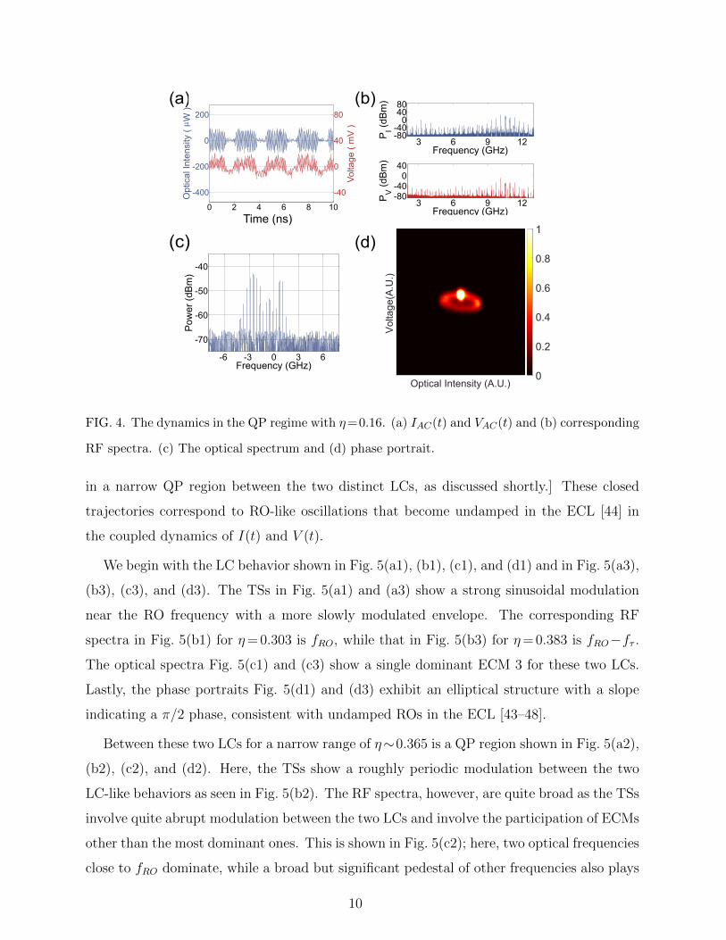
periodic, as seen in Fig. 4(a). The RF frequencies contributing to the TSs are concentrated

above ∼8 GHz, shown in Fig. 4(b). Many active ECMs (∼ −10 to 4) participate, as seen in

Fig. 4(c).

The observed QP dynamics can be described as a periodic switching between CW (con-

8

Optical Intensity (A.U.)V

olta

ge(A

.U.)

0

0.2

0.4

0.6

0.8

1

-400

-200

0

200

Opt

ical

Inte

nsity

( μ

W )

0 2 4 6 8 10

-40

0

40

80

Vol

tage

( m

V )

3 6 9 12-80-40

04080

PI (

dBm

)

Frequency (GHz)

3 6 9 12-80-40

040

PV (

dBm

)

Frequency (GHz)

-6 -3 0 3 6

-70

-60

-50

-40

Frequency (GHz)

Pow

er (

dBm

)

(a) (b)

(c)

Time (ns)

(d)

FIG. 3. The dynamics in the CW regime with η=0. (a) IAC(t) and VAC(t) and (b) corresponding

RF spectra. (c) The optical spectrum and (d) phase portrait.

stant) and limit-cycle (LC) (oscillatory) behaviors (a LC is a closed trajectory in phase

space); the LC-like behavior which originates from ROs, becomes more dominant as η in-

creases across this range with the intervals of CW-like behavior becoming relatively shorter.

In Fig. 4(d) we see the corresponding phase portrait. There is a central broadened bright

spot corresponding to the CW-like behavior and a ring-shaped feature corresponding to the

LC-like behavior.

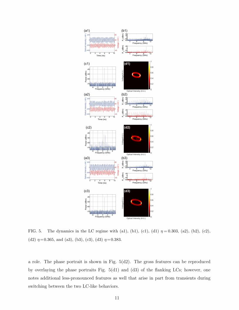
Multiple limit cycles

At η=0.29, the ECL undergoes a bifurcation into a LC regime [47, 49]; at this point, CW-

like behavior no longer appears. Several LCs are observed for various η in this regime, as seen

in the region labelled LC in Fig. 2(b) where, apart from narrow ranges of η, the BD exhibits

two high-density features for a given η consistent with the approximately sinusoidal behavior

of the corresponding TSs as discussed below. Two such LCs are shown in Fig. 5(a1) (TSs),

(b1) (RF spectra), (c1) (optical spectrum), and (d1) (phase portrait) and in Fig. 5(a3), (b3),

(c3), and (d3). [Figure 5(a2), (b2), (c2), and (d2), however, show the corresponding plots

9

3 6 9 12-80-40

04080

PI (

dBm

)

Frequency (GHz)

3 6 9 12-80-40

040

PV (

dBm

)

Frequency (GHz)

-6 -3 0 3 6

-70

-60

-50

-40

Frequency (GHz)

Pow

er (

dBm

)

(a) (b)

(c)

-400

-200

0

200

Opt

ical

Inte

nsity

( μ

W )

0 2 4 6 8 10

-40

0

40

80

Vol

tage

( m

V )

Time (ns)

Optical Intensity (A.U.)V

olta

ge(A

.U.)

0

0.2

0.4

0.6

0.8

1(d)

FIG. 4. The dynamics in the QP regime with η=0.16. (a) IAC(t) and VAC(t) and (b) corresponding

RF spectra. (c) The optical spectrum and (d) phase portrait.

in a narrow QP region between the two distinct LCs, as discussed shortly.] These closed

trajectories correspond to RO-like oscillations that become undamped in the ECL [44] in

the coupled dynamics of I(t) and V (t).

We begin with the LC behavior shown in Fig. 5(a1), (b1), (c1), and (d1) and in Fig. 5(a3),

(b3), (c3), and (d3). The TSs in Fig. 5(a1) and (a3) show a strong sinusoidal modulation

near the RO frequency with a more slowly modulated envelope. The corresponding RF

spectra in Fig. 5(b1) for η= 0.303 is fRO, while that in Fig. 5(b3) for η= 0.383 is fRO−fτ .

The optical spectra Fig. 5(c1) and (c3) show a single dominant ECM 3 for these two LCs.

Lastly, the phase portraits Fig. 5(d1) and (d3) exhibit an elliptical structure with a slope

indicating a π/2 phase, consistent with undamped ROs in the ECL [43–48].

Between these two LCs for a narrow range of η∼0.365 is a QP region shown in Fig. 5(a2),

(b2), (c2), and (d2). Here, the TSs show a roughly periodic modulation between the two

LC-like behaviors as seen in Fig. 5(b2). The RF spectra, however, are quite broad as the TSs

involve quite abrupt modulation between the two LCs and involve the participation of ECMs

other than the most dominant ones. This is shown in Fig. 5(c2); here, two optical frequencies

close to fRO dominate, while a broad but significant pedestal of other frequencies also plays

10

-6 -3 0 3 6

-70

-60

-50

-40

Frequency (GHz)

Pow

er (

dBm

)

Time (ns)

-400

-200

0

200

Opt

ical

Inte

nsity

( μ

W )

0 2 4 6 8 10

-40

0

40

80

Vol

tage

( m

V )

-400

-200

0

200

Opt

ical

Inte

nsity

( μ

W )

0 2 4 6 8 10

-40

0

40

80

Vol

tage

( m

V )

3 6 9 12-80-40

04080

PI (

dBm

)

Frequency (GHz)

3 6 9 12-80-40

040

PV (

dBm

)

Frequency (GHz)

3 6 9 12-80-40

04080

PI (

dBm

)

Frequency (GHz)

3 6 9 12-80-40

040

PV (

dBm

)

Frequency (GHz)

-6 -3 0 3 6

-70

-60

-50

-40

Frequency (GHz)

Pow

er (

dBm

)

(a2)

(c2)

Time (ns)

3 6 9 12-80-40

04080

PI (

dBm

)

Frequency (GHz)

3 6 9 12-80-40

040

PV (

dBm

)

Frequency (GHz)

-6 -3 0 3 6

-70

-60

-50

-40

Frequency (GHz)

Pow

er (

dBm

)

-400

-200

0

200

Opt

ical

Inte

nsity

( μ

W )

0 2 4 6 8 10

-40

0

40

80

Vol

tage

( m

V )

Time (ns)

Optical Intensity (A.U.)

Vol

tage

(A.U

.)

0

0.2

0.4

0.6

0.8

1

Optical Intensity (A.U.)

Vol

tage

(A.U

.)

0

0.2

0.4

0.6

0.8

1

Optical Intensity (A.U.)

Vol

tage

(A.U

.)

0

0.2

0.4

0.6

0.8

1

(a1) (b1)

(c1)

(a3) (b3)

(c3)

(d2)

(d1)

(d3)

(b2)

FIG. 5. The dynamics in the LC regime with (a1), (b1), (c1), (d1) η = 0.303, (a2), (b2), (c2),

(d2) η=0.365, and (a3), (b3), (c3), (d3) η=0.383.

a role. The phase portrait is shown in Fig. 5(d2). The gross features can be reproduced

by overlaying the phase portraits Fig. 5(d1) and (d3) of the flanking LCs; however, one

notes additional less-pronounced features as well that arise in part from transients during

switching between the two LC-like behaviors.

11

Subharmonic

As η is increased into the range 0.4-0.52, the ECL is characterized by SH dynamics [23–

25]. By SH we mean that the TSs are dominated by two (or more) frequencies that sum to

fRO±mfτ with m an integer. In selected cases, we shall find it useful to plot phase portraits

obtained from relatively short-duration TSs to differentiate qualitatively different behaviors

that contribute to the SH dynamics at a given η. This will enable us to gain insight into

what portions of the trajectory are associate with which RF frequencies.

Figure 6 shows (a) the TSs, (b) the RF spectra, (c) the optical spectra, and the phase

portrait (d) with short-duration TSs [0.4 ns] and (e) long-duration [25 µ second] TSs. The

TSs, shown in Fig. 6(a) exhibit oscillations near fRO, that are themselves modulated at

roughly fRO/2 indicating a beating between two frequencies close to fRO. This is supported

by the appearance in Fig. 6 (b) of two dominant peaks in the RF spectra with frequencies

f1 =3.66 GHz and f2 =6.5 GHz (other weaker peaks also appear); note that f1+f2 =fRO=

10.16 GHz. The phase portrait using relatively short-duration TSs in Fig. 6 (d) emphasizes

the nature of the dynamics. In Fig. 6 (e) we see two open structures that repeat in succession,

that can be distinguished as the green and blue portions of the phase portrait in Fig. 6 (d)

and corresponding shaded regions of Fig. 6(a). The RF frequency [Fig. 6(b)], f1 =3.66 GHz

corresponds to the green structure and f2 =6.5 GHz corresponds to the blue structure.

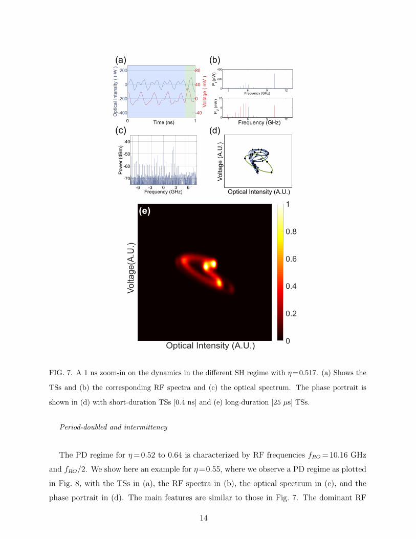
Figure 7 shows an example restricting our view to a different SH behavior for η=0.517.

In Fig. 7 (a) a shorter timescale is shown (1 ns) compared with that used in previous figures.

The TSs appear roughly as sinusoidal modulated by an envelope at half the dominant

frequency of the sinusoid [more apparent in the TS for I(t)]. This is the signature of the

PD regime. What is evident from the TSs is born out in the RF spectra in Fig. 7(b).

Here we see a dominant peak at fRO and a cluster of peaks near fRO/2. Figures 7(d)

and (e) show the corresponding phase portraits, for (d) short-duration TSs [0.4 ns] and (e)

long-duration [25 µs] TSs. Compared with what was seen in the SH regime at somewhat

smaller η, far more time is spent on the blue trace and shaded region with (irregularly

shaped) features reminiscent of PD dynamics than on the green trace and shaded region

with features resembling behavior in the LC regime discussed above, in Fig. 7 (a) and (d).

The RF spectrum corresponding to Fig. 7(b) shows a dominant peak at fRO = 10.16 GHz

while the TSs in stable PD have dominant peak at fRO + fτ = 10.56. A smoothed curve

12

3 6 9 12

300

600

P I (μ

W)

Frequency (GHz)

3 6 9 12

20

40

PV (

mV

)

Frequency (GHz)

(b)

(d)

Optical Intensity (A.U.)

Vol

tage

(A.U

.)

0

0.2

0.4

0.6

0.8

1(e)

Optical Intensity (A.U.)

Vol

tage

(A

.U.)

(d)

-6 -3 0 3 6

-70

-60

-50

-40

Frequency (GHz)

Pow

er (

dBm

)

(c)

-400

-200

0

200

Opt

ical

Inte

nsity

(W

)

-40

0

40

80

Vol

tage

(mV

)

(a)

Time (ns)0 1

FIG. 6. A 1 ns zoom-in on the dynamics in the SH regime with η=0.497. (a) Shows the TSs and

(b) the corresponding RF spectra and (c) the optical spectrum. The phase portrait is shown in

(d) with short-duration TSs [0.4 ns] and (e) long-duration [25 µs] TSs.

connecting both regimes where the green (blue) curve is determined to be LC (PD). The two

trajectories are mapped on the phase portrait in Fig. 7(d) where the PD regime is plotted

in blue; and the LC trajectory is plotted in green. The diamonds (circles) are the raw data

from the TSs. Lastly, the corresponding phase portrait for long TSs is shown in Fig. 7(e).

13

Optical Intensity (A.U.)

Vol

tage

(A.U

.)

0

0.2

0.4

0.6

0.8

1

3 6 9 120

200

400

PI (μ

W)

Frequency (GHz)

3 6 9 120

5

10

PV (

mV

)

Frequency (GHz)

(b)

-400

-200

0

200

Opt

ical

Inte

nsity

( μ

W )

0 1

-40

0

40

80

Vol

tage

( m

V )

Time (ns)

(a)

-6 -3 0 3 6

-70

-60

-50

-40

Frequency (GHz)

Pow

er (

dBm

)

(c)

(e)

Optical Intensity (A.U.)

Vol

tage

(A

.U.)

(d)

FIG. 7. A 1 ns zoom-in on the dynamics in the different SH regime with η=0.517. (a) Shows the

TSs and (b) the corresponding RF spectra and (c) the optical spectrum. The phase portrait is

shown in (d) with short-duration TSs [0.4 ns] and (e) long-duration [25 µs] TSs.

Period-doubled and intermittency

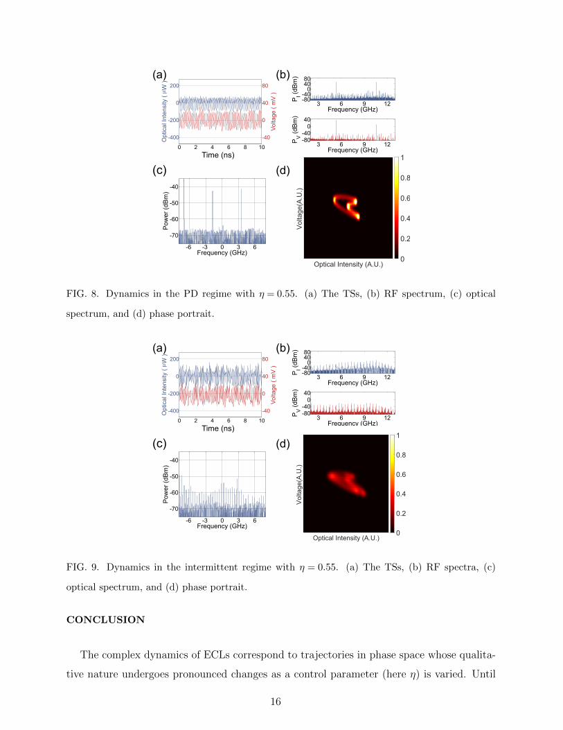
The PD regime for η= 0.52 to 0.64 is characterized by RF frequencies fRO = 10.16 GHz

and fRO/2. We show here an example for η=0.55, where we observe a PD regime as plotted

in Fig. 8, with the TSs in (a), the RF spectra in (b), the optical spectrum in (c), and the

phase portrait in (d). The main features are similar to those in Fig. 7. The dominant RF

14

frequencies in Fig. 8(b) are fRO+fτ = 10.56 GHz and (fRO+fτ )/2 = 5.28 GHz compared

with fRO = 10.16 GHz and fRO/2 = 5.08 GHz in Fig. 7. Note that even though the phase

portrait shown in Fig. 8(d) has similar overall shape as the phase portrait (green) in Fig.

7(b), the two TSs do not have the same dominant RF frequencies. The transition of the

dynamical behavior varies from SH to PD involves the formation of a stable solution. The

RF peak in SH is found to be fτ + fRO and the trajectories are comprised of an LC and

a PD, as the feedback strength increases. As feedback is increased, we find the duration of

PD increases, and the trajectories become more dominant until PD takes over and the new

solution is found to be PD with RF peak at fRO.

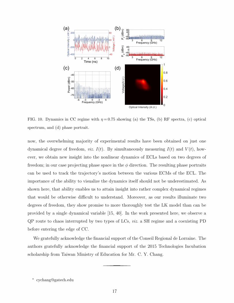
We illustrate intermittency at η = 0.545 which is evident within a single TS shown in

Fig. 9 and the animation in the supplement material. This type of intermittency has been

investigated in Ref. [26], we can identify chaotic and PD along with other complex dynamics

shown in Figs. 9(a)-(d). The sequential order of the dynamics in this TS appear to be random

which can be found in the animation in the supplement material. We see considerable

broadening of the features compared with the PD phase portrait in Fig. 7. The phase

portrait exhibits an overall elliptical structure (LC-like behavior) together with enhanced

density in the upper right of the phase portrait associated with PD-like behavior, with

considerably more time spent on the PD-like phase (∼35:1). A more detailed examination

of the phase portrait over many shorter duration TSs bears out this interpretation. The

PD-like dynamics here differ somewhat from those shown in Fig. 8.

Coherence collapse

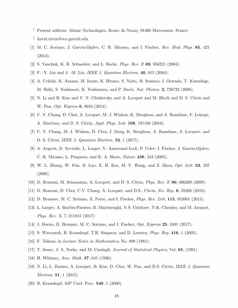
As η is further increased above 0.64 the onset of chaos is reached. An example for η=0.75

is shown in Fig. 10. In this regime, the BDs of Fig. 2(a) and (b) are quite broadened in the

vertical direction indicating many maxima and minima in the respective TSs as well as the

participation of numerous ECMs [Fig. 2(c)]. The TSs [Fig. 10(a)] become quite complex

and involve a very broad range of RF frequencies [Fig. 10(b)]. Likewise, many ECMs

participate in the dynamics [Fig. 10(c)]. The phase portrait [Fig. 10(d)], consequently,

has an undifferentiated broadened feature with a hint of elliptical structure (reflecting the

continues role of RO oscillations).

15

-400

-200

0

200

Opt

ical

Inte

nsity

( μ

W )

0 2 4 6 8 10

-40

0

40

80

Vol

tage

( m

V )

-6 -3 0 3 6

-70

-60

-50

-40

Frequency (GHz)

Pow

er (

dBm

)

Optical Intensity (A.U.)

Vol

tage

(A.U

.)

(d)

(a) (b)

(c)Time (ns)

3 6 9 12-80-40

04080

PI (

dBm

)

Frequency (GHz)

3 6 9 12-80-40

040

PV (

dBm

)

Frequency (GHz)

0

0.2

0.4

0.6

0.8

1

FIG. 8. Dynamics in the PD regime with η = 0.55. (a) The TSs, (b) RF spectrum, (c) optical

spectrum, and (d) phase portrait.

-400

-200

0

200

Opt

ical

Inte

nsity

( μ

W )

0 2 4 6 8 10

-40

0

40

80

Vol

tage

( m

V )

-6 -3 0 3 6

-70

-60

-50

-40

Frequency (GHz)

Pow

er (

dBm

)

3 6 9 12-80-40

04080

PI (

dBm

)

Frequency (GHz)

3 6 9 12-80-40

040

PV (

dBm

)

Frequency (GHz)

Optical Intensity (A.U.)

Vol

tage

(A.U

.)

0

0.2

0.4

0.6

0.8

1

(a) (b)

(c)Time (ns)

(d)

FIG. 9. Dynamics in the intermittent regime with η = 0.55. (a) The TSs, (b) RF spectra, (c)

optical spectrum, and (d) phase portrait.

CONCLUSION

The complex dynamics of ECLs correspond to trajectories in phase space whose qualita-

tive nature undergoes pronounced changes as a control parameter (here η) is varied. Until

16

Optical Intensity (A.U.)

Vol

tage

(A.U

.)

0

0.2

0.4

0.6

0.8

1(d)

3 6 9 12-80-40

04080

PI (

dBm

)

Frequency (GHz)

3 6 9 12-80-40

040

PV (

dBm

)

Frequency (GHz)

-6 -3 0 3 6

-70

-60

-50

-40

Frequency (GHz)

Pow

er (

dBm

)

-400

-200

0

200

Opt

ical

Inte

nsity

( μ

W )

0 2 4 6 8 10

-40

0

40

80

Vol

tage

( m

V )

(a) (b)

(c)Time (ns)

FIG. 10. Dynamics in CC regime with η= 0.75 showing (a) the TSs, (b) RF spectra, (c) optical

spectrum, and (d) phase portrait.

now, the overwhelming majority of experimental results have been obtained on just one

dynamical degree of freedom, viz. I(t). By simultaneously measuring I(t) and V (t), how-

ever, we obtain new insight into the nonlinear dynamics of ECLs based on two degrees of

freedom; in our case projecting phase space in the φ direction. The resulting phase portraits

can be used to track the trajectory’s motion between the various ECMs of the ECL. The

importance of the ability to visualize the dynamics itself should not be underestimated. As

shown here, that ability enables us to attain insight into rather complex dynamical regimes

that would be otherwise difficult to understand. Moreover, as our results illuminate two

degrees of freedom, they show promise to more thoroughly test the LK model than can be

provided by a single dynamical variable [15, 40]. In the work presented here, we observe a

QP route to chaos interrupted by two types of LCs, viz. a SH regime and a coexisting PD

before entering the edge of CC.

We gratefully acknowledge the financial support of the Conseil Regional de Lorraine. The

authors gratefully acknowledge the financial support of the 2015 Technologies Incubation

scholarship from Taiwan Ministry of Education for Mr. C. Y. Chang.

∗ cychang@gatech.edu

17

† Present address: Almae Technologies, Route de Nozay, 91460 Marcoussis- France

‡ david.citrin@ece.gatech.edu

[1] M. C. Soriano, J. Garcıa-Ojalvo, C. R. Mirasso, and I. Fischer, Rev. Mod. Phys. 85, 421

(2013).

[2] S. Yanchuk, K. R. Schneider, and L. Recke, Phys. Rev. E 69, 056221 (2004).

[3] F. -Y. Lin and J. -M. Liu, IEEE J. Quantum Electron. 40, 815 (2004).

[4] A. Uchida, K. Amano, M. Inoue, K. Hirano, S. Naito, H. Someya, I. Oowada, T. Kurashige,

M. Shiki, S. Yoshimori, K. Yoshimura, and P. Davis, Nat. Photon. 2, 728732 (2008).

[5] N. Li and B. Kim and V. N. Chizhevsky and A. Locquet and M. Bloch and D. S. Citrin and

W. Pan, Opt. Express 6, 6634 (2014).

[6] C. Y. Chang, D. Choi, A. Locquet, M. J. Wishon, K. Merghem, and A. Ramdane, F. Lelarge,

A. Martinez, and D. S. Citrin, Appl. Phys. Lett. 108, 191109 (2016).

[7] C. Y. Chang, M. J. Wishon, D. Choi, J. Dong, K. Merghem, A. Ramdane, A. Locquet, and

D. S. Citrin, IEEE J. Quantum Electron. 53, 1 (2017).

[8] A. Argyris, D. Syvridis, L. Larger, V. Annovazzi-Lodi, P. Colet, I. Fischer, J. Garcia-Ojalvo,

C. R. Mirasso, L. Pesquera, and K. A. Shore, Nature 438, 343 (2005).

[9] W. L. Zhang, W. Pan, B. Luo, X. H. Zou, M. Y. Wang, and Z. Zhou, Opt. Lett. 33, 237

(2008).

[10] D. Rontani, M. Sciamanna, A. Locquet, and D. S. Citrin, Phys. Rev. E 80, 066209 (2009).

[11] D. Rontani, D. Choi, C.Y. Chang, A. Locquet, and D.S., Citrin, Sci. Rep. 6, 35206 (2016).

[12] D. Brunner, M. C. Soriano, X. Porte, and I. Fischer, Phys. Rev. Lett. 115, 053901 (2015).

[13] L. Larger, A. Baylon-Fuentes, R. Martinenghi, V.S. Udaltsov, Y.K. Chembo, and M. Jacquot,

Phys. Rev. X, 7, 011015 (2017)

[14] J. Bueno, D. Brunner, M. C. Soriano, and I. Fischer, Opt. Express 25, 2401 (2017).

[15] S. Wieczorek, B. Krauskopf, T.B. Simpson, and D. Lenstra, Phys. Rep. 416, 1 (2005).

[16] F. Takens, in Lecture Notes in Mathematics, No. 898 (1981).

[17] T. Sauer, J. A. Yorke, and M. Casdagli, Journal of Statistical Physics, Vol. 65, (1991)

[18] H. Whitney, Ann. Math. 37, 645 (1936).

[19] N. Li, L. Zunino, A. Locquet, B. Kim, D. Choi, W. Pan, and D.S. Citrin, IEEE J. Quantum

Electron. 51, 1 (2015)

[20] B. Krauskopf, AIP Conf. Proc. 548, 1 (2000).

18

[21] R. Lang and K. Kobayashi, IEEE J. Quantum Electron. 16, 347 (1980).

[22] B. Tromborg and J. Mork, IEEE Photon. Technol. Lett. 2, 549 (1990).

[23] T. Mukai, and K. Otsuka, Phys. Rev. Lett. 55, 1711 (1985).

[24] Y. H. Kao, N. M. Wang, and H. M. Chen, IEEE J. Quantum Electron. 30, 1732 (1994).

[25] M. Ahmed, M. Yamada, and S. Abdulrhmann, Int. J NUMER. MODEL. EL. 22, 434 (2009).

[26] A. E. Hramov, A. A. Koronovskii, O. I. Moskalenko, M. O. Zhuravlev, R. Jaimes-Reategui,

and A. N. Pisarchik, Phys. Rev. E 93, 052218, (2016).

[27] J. Mork , J. Mark, and B. Tromborg, Phys. Rev. Lett. 65, 1999 (1990).

[28] A. Hohl, and A. Gavrielides, Phys. Rev. Lett., 82 1148 (1999).

[29] H. Li and J. Ye and J. G. McInerney, IEEE J. Quant. Electron. 29, 2121 (1993).

[30] B. Kim, N. Li, A. Locquet, and D. S. Citrin, Opt. Express 22, 2348 (2014).

[31] B. Kim, A. Locquet, N. Li, D. Choi, and D. S. Citrin, IEEE J. Quantum Electron. 50, 965

(2014).

[32] B. Kim, A. Locquet, D. Choi, and D. S. Citrin, Phys. Rev. A 91, 061802 (2015).

[33] Ref. [12] maps all three dynamical variables simultaneously in the LFF regime for an ECL.

In our work, we consider more broadly the route to chaos in an ECL. Moreover, the route to

chaos in our ECL is a different route (commented upon in the body of our paper) and does

not involve LFF.

[34] A. Locquet, B. Kim, D. Choi, N. Li, and D. S. Citrin, Phys. Rev. A 95, 023801 (2017).

[35] W. Ray, W. S. Lam, P. N. Guzdar, and R. Roy, Phys. Rev. E 73, 026219 (2006).

[36] A. A. Sahai, B. Kim, D. Choi, A. Locquet, and D. S. Citrin, Opt. Lett. 39, 5630, (2014).

[37] R. F. Kazarinov and R. Suris, Sov. Phys.-JETP 39, 522 (1974).

[38] Note, however, that Ref. [12] has experimentally determined trajectories in the LFF regime

while numerous works utilizing ECLs as feedback sensors have monitored V in a static fashion.

See, for example M.J. Wishon, A. Locquet, G. Mourozeau, D. Choi, Sreejith K.R., A.A. Sahai,

and D.S. Citrin, IET Optoelectronics (2017), in press.

[39] C. Masoller and N. B. Abraham, Phys. Rev. A 57, 1313 (1998).

[40] S. Wieczorek, T.B. Simpson, B. Krauskopf, and D. Lenstra, Opt. Commun. 215, 125 (2003).

[41] Q. Zou, K. Merghem, S. Azouigui, A. Martinez, A. Accard, N. Chimot, F. Lelarge, and A.

Ramdane, Appl. Phys. Lett. 97, 231115 (2010).

[42] Yariv, A. and Yeh, P., (2007). Photonics: optical electronics in modern communications (Vol.

19

6). New York: oxford university press.

[43] B. Tromborg, J.H. Edmundson, and H. Olesen, IEEE J. Quantum Electron. QE-20, 1023

(1984).

[44] J.S. Cohen, R.R. Drenten, and B.H. Verbeek, , IEEE J. Quantum Electron. QE-24, 1989

(1988).

[45] N. Schunk and K. Peterman, IEEE J. Quantum Electron. QE-24, 1242 (1988).

[46] J. Helms and K. Peterman, IEEE J. Quantum Electron. QE-26, 833 (1990).

[47] A. Ritter and H. Haug, J. Opt. Soc. Am. 1, 145 (1993).

[48] G.H.M. van Tartwijk and D. Lenstra, Phys. Rev. A 50, 2837 (1994).

[49] A. Ritter and H. Haug, IEEE J. Quantum Electron. 29, 1064 (1993).

[50] X. Porte, M. C. Soriano, and I. Fischer,Phys. Rev. A 89, 023822 (2014).

[51] N. Li, A. Locquet, and D. S. Citrin, Opt. Lett. 40, 6634 (2015).

20