Volume xx(200y), Number z, pp. 1–12

Visualizing Strain Anisotropy in Mantle Flow Fields

H. Obermaier1, M. I. Billen1, H. Hagen2, M. Hering-Bertram3, and B. Hamann1

1University of California, Davis, USA2University of Kaiserslautern, Germany

3Rhine-Waal University of Applied Sciences, Germany

AbstractThe evolution of strain and development of material anisotropy in models of Earth’s mantle flow convey importantinformation about how to interpret the geometric relationship between observation of seismic anisotropy and theactual mantle flow field. By combining feature extraction techniques such as path line integration and tensor accu-mulation, we compute time-varying strain vector fields thatbuild the foundation for a number of feature extractionand visualization techniques. The proposed field segmentation, clustering, histograms, and multi-volume visual-ization techniques facilitate an intuitive understandingof three-dimensional strain in such flow fields, overcominglimitations of previous methods such as 2D line plots and slicing. We present applications of our approach to anartificial time varying flow data set and a real world example of stationary flow in a subduction zone and discussthe challenges of processing these geophysical data sets aswell as the insights gained.

Categories and Subject Descriptors(according to ACM CCS): I.6.6 [Computer Graphics]: Simulation OutputAnalysis—

1. Introduction

Vector field visualization has received strong attention intherecent history of scientific visualization, as flow simulationtechniques have become available to a diverse set of applica-tion areas. While the best known application fields for flowsimulation such as aerodynamics and industrial mixing havebeen studied extensively from a visualization point of view,other fields such as geophysics suffer from a lack of specificvisualization techniques and require the definition and devel-opment of alternative and tailor-made visualization methods.

Solid Earth geodynamics is concerned with the forces thatmove tectonic plates at the planet’s surface through energyprovided by solid-state thermo-chemical convection in themantle (outer 2890 km). Over long periods of time (> 10,000- 1 million years) and at the high temperatures and pressuresof the mantle, material deforms by a process of solid-statecreep flow at high effective viscosity (1019 - 1025 Pa-s). Dueto the long time-scales and slow (< 10 - 100 cm/yr) non-inertial flow resulting from the high viscosity, the point ofinterest shifts away from classic flow field illustration, suchas integral structure and vortex core extraction, towards vi-sualization of more general continuum mechanics including

object deformation, and the applicability of generic flow vi-sualization techniques is rather limited.

In this paper, we are concerned with upper mantle flow (<670 km depth) in subduction zones, where one tectonic platesinks beneath another tectonic plate (e.g., Alaska, Japan).These subduction zones are of high importance to geosci-entists because they provide the largest forces driving platetectonics and are the most seismically active regions on theplanet. One of the major outstanding questions regardingsubduction zones is the geometry of mantle flow inducedby sinking of a dense tectonic plate into the mantle [Bil08],which cannot be observed directly. Observations of seis-mic anisotropy provide indirect evidence of this pattern, be-cause the crystal axis of the seismically anisotropic mineralolivine will align (i.e., they form a lattice preferred orien-tation (LPO)) with the strain direction during deformation.However, these observations must be interpreted with the aidof simulations of mantle flow, which track the evolution ofstrain and material alignment.

Our work aims at solving the problem of 3D flow-inducedstrain analysis by integrating a combination of feature ex-traction and field processing techniques with novel methodsof strain segmentation and visualization. The resulting visu-

submitted to COMPUTER GRAPHICSForum(7/2011).

2 Obermaier et al. / Visualizing Strain Anisotropy in Mantle Flow Fields

alization of flow and strain helps geoscientists in two ways.Firstly, it allows the scientist to distinguish regions with uni-form strain orientations, which can be analyzed with a sim-ple algorithm for comparison to observations, from morecomplex regions requiring more detailed analysis. Secondly,it facilitates rapid identification of the relative orientation ofthe strain orientations and the flow-field, which provides formore accurate interpretation of seismic anisotropy observa-tions to determine the flow field. As a consequence, our workcontributes both to the application field of geophysics byproviding an intuitive and interactive visualization for flowinduced strain analysis as well as to the visualization com-munity by introducing novel methods for non-directed strainaxis field segmentation and strain and cluster visualization.

The remainder of this paper is structured as follows: Sec-tion 2 gives an overview of existing visualization methodsin the area of geophysics and strain visualization. In Sec-tion 3, background information on geological subductionand data formats are provided. Section 4 details the stepsof strain field computation. Segmentation and visualizationof the resulting strain fields are explained in detail in Sec-tions 5 and 6. This is followed by an application and resultssection presenting the created results and their benefits forthe geophysics community. Section 8 concludes this paper.

2. Related Work

Work related to the scope of this paper can be found in thefield of visualization, where it is centered on visualization ofvector and tensor fields and is partially related to strain anal-ysis and in the field of geophysics, where basic techniquesare used for visual analysis of flow and strain data.

Visualization Different flow visualization techniques arerelated to properties of flow induced strain. One such methodis the Finite Time Lyapunov Exponent(FTLE) [Hal01]which derives a scalar valued convergence and divergencemap from flow fields. The maximal structures of this fieldhighlight regions where strain along a particle trajectoryislocally maximal, thus giving an insight into flow separa-tion. Contrary to FTLE, which is based on gridded inte-gral line generation, others [OHBKH09] have proposed vi-sualizing strain that was accumulated along individual in-tegral flow lines to visualize deformation of distinct vol-ume particles over time. This technique has recently beenapplied to generate a localized FTLE map [KPH∗09]. Thework presented in this paper makes use of a similarly denseand localized line integration to obtain strain directionsintime-varying flow fields. In tensor field visualization andDiffusion Tensor Imagingin particular, anisotropy cluster-ing based on tensor invariants with varying distance mea-sures is state-of-the-art and has been proposed by severalauthors [ZMB∗03, STS07, RJF∗09]. Their clustering meth-ods are fine tuned for DT-MRI tensor fields. In the contextof geophysics, stress-related tensors have been visualized

by glyphs in [NJP05]. In the last years, strain segmentationhas received increased attention in vector field visualizationby the definition of various Eulerian and Lagrangian strainmeasures, which have been used to segment flow fields intostrain and vortex regions based on the magnitude of thesecomponents [SWTH07]. For a state-of-the-art report on vol-ume visualization we refer to [EHK∗04].

Geophysics Analysis of Lattice Preferred Orientationorgrain orientation [ZiK95] obtained from mantle flow simu-lations of subduction zones [JB10,WSMG06] is commonlyperformed by manual inspection of generic visualizations re-sulting from techniques such as slicing and arrow plot visu-alization [JB10] of instantaneousInfinite Strain Axisdirec-tions [JB10, KR02]. While these visualization methods aregenerally available and easy to implement, they suffer fromloss of dimension and lack a homogeneous field impression.The need of manual parameter adjustment such as slicingorientation and position favors overlooking of features dur-ing visual inspection. A first attempt at computing and inter-preting LPO from time-varying flow simulations was donein [MvKK02] by the integration of strain along particle trac-ers. The resulting two-dimensional strain orientation field isvisualized using line plots and temperature based coloringand serves as basis for further manual analysis and segmen-tation. Work with focus on visualization of geophysical flowwith analysis of heat and critical point development is givenby [EYD02]. A natural two-dimensional watershed-like vi-sualization of LPO is given by optical micrographs with po-larized light [ZiK95] and is the result of photographing phys-ically sliced material samples in lab experiments. FTLE-likevisualizations are presented in [Sub09].

3. Strain in Geophysical Flow Data

In simple flow fields, such as horizontally oriented simpleshear found beneath the center of large tectonic plates, itis appropriate to assume that the orientation of LPO, orobserved seismic anisotropy, and the flow field is paral-lel [CBS07]. However, in subduction zones, the flow-fieldcan be highly three-dimensional depending on the geome-try of the subducting plate [JB10] and can change rapidly intime [BB10]. An observation of seismic anisotropy providesa single measurement at the Earth’s surface that reflects thechanging pattern of seismic anisotropy along the ray path ofthe seismic wave in the upper mantle, as illustrated in Figure1. Therefore, accurate interpretation of this observation re-quires knowing how the pattern of material alignment variesspatially and how it relates to the geometry of the flow field.

3.1. Background

Simulation of subducting slab movement and evolution ofLPOs enables geophysicists to make predictions about thepropagation of seismic waves caused by earthquakes or ar-tificial sources. Observation of differences in the speed of

submitted to COMPUTER GRAPHICSForum(7/2011).

Obermaier et al. / Visualizing Strain Anisotropy in Mantle Flow Fields 3

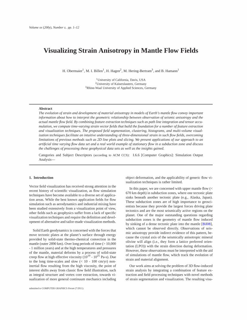
Figure 1: A seismic wave travels through the Earth’s mantlebefore reaching a sensor at the surface. LPO along the ray (inblue) are used as approximation of mantle flow geometry.

propagation of polarized seismic waves is one method ofinferring the pattern of mantle flow [RS94]. Such seismicanisotropy occurs in the upper mantle in regions where de-formation causes the crystal lattice within olivine minerals toacquire a preferred orientation. Bulk alignment of this min-eral’s crystal structure will cause seismic waves that travelthrough these regions to arrive at seismic stations at differenttimes depending on wave polarization. From this informa-tion seismologists can geographically map bulk alignmentin the mantle, which is usually indicated by plotting the di-rection of the fastest seismic axis of the olivine mineral, pro-viding a first rough approximation of mantle flow directions.

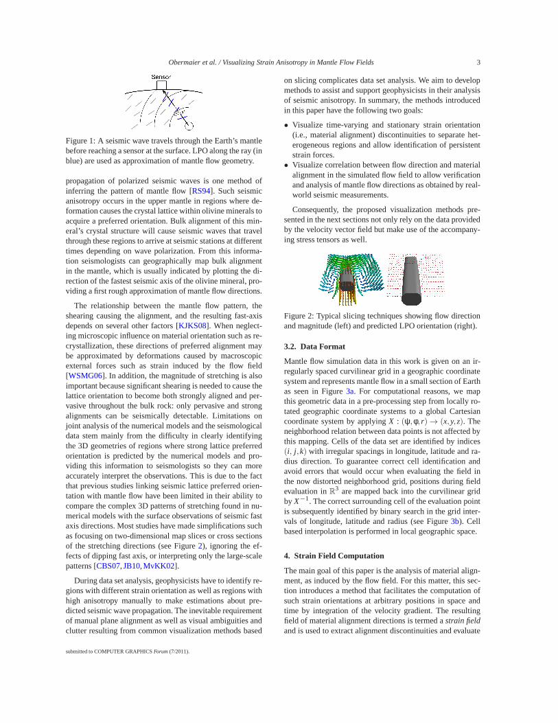
The relationship between the mantle flow pattern, theshearing causing the alignment, and the resulting fast-axisdepends on several other factors [KJKS08]. When neglect-ing microscopic influence on material orientation such as re-crystallization, these directions of preferred alignmentmaybe approximated by deformations caused by macroscopicexternal forces such as strain induced by the flow field[WSMG06]. In addition, the magnitude of stretching is alsoimportant because significant shearing is needed to cause thelattice orientation to become both strongly aligned and per-vasive throughout the bulk rock: only pervasive and strongalignments can be seismically detectable. Limitations onjoint analysis of the numerical models and the seismologicaldata stem mainly from the difficulty in clearly identifyingthe 3D geometries of regions where strong lattice preferredorientation is predicted by the numerical models and pro-viding this information to seismologists so they can moreaccurately interpret the observations. This is due to the factthat previous studies linking seismic lattice preferred orien-tation with mantle flow have been limited in their ability tocompare the complex 3D patterns of stretching found in nu-merical models with the surface observations of seismic fastaxis directions. Most studies have made simplifications suchas focusing on two-dimensional map slices or cross sectionsof the stretching directions (see Figure2), ignoring the ef-fects of dipping fast axis, or interpreting only the large-scalepatterns [CBS07,JB10,MvKK02].

During data set analysis, geophysicists have to identify re-gions with different strain orientation as well as regions withhigh anisotropy manually to make estimations about pre-dicted seismic wave propagation. The inevitable requirementof manual plane alignment as well as visual ambiguities andclutter resulting from common visualization methods based

on slicing complicates data set analysis. We aim to developmethods to assist and support geophysicists in their analysisof seismic anisotropy. In summary, the methods introducedin this paper have the following two goals:

• Visualize time-varying and stationary strain orientation(i.e., material alignment) discontinuities to separate het-erogeneous regions and allow identification of persistentstrain forces.

• Visualize correlation between flow direction and materialalignment in the simulated flow field to allow verificationand analysis of mantle flow directions as obtained by real-world seismic measurements.

Consequently, the proposed visualization methods pre-sented in the next sections not only rely on the data providedby the velocity vector field but make use of the accompany-ing stress tensors as well.

Figure 2: Typical slicing techniques showing flow directionand magnitude (left) and predicted LPO orientation (right).

3.2. Data Format

Mantle flow simulation data in this work is given on an ir-regularly spaced curvilinear grid in a geographic coordinatesystem and represents mantle flow in a small section of Earthas seen in Figure3a. For computational reasons, we mapthis geometric data in a pre-processing step from locally ro-tated geographic coordinate systems to a global Cartesiancoordinate system by applyingX : (ψ,φ, r)→ (x,y,z). Theneighborhood relation between data points is not affected bythis mapping. Cells of the data set are identified by indices(i, j ,k) with irregular spacings in longitude, latitude and ra-dius direction. To guarantee correct cell identification andavoid errors that would occur when evaluating the field inthe now distorted neighborhood grid, positions during fieldevaluation inR3 are mapped back into the curvilinear gridby X−1. The correct surrounding cell of the evaluation pointis subsequently identified by binary search in the grid inter-vals of longitude, latitude and radius (see Figure3b). Cellbased interpolation is performed in local geographic space.

4. Strain Field Computation

The main goal of this paper is the analysis of material align-ment, as induced by the flow field. For this matter, this sec-tion introduces a method that facilitates the computation ofsuch strain orientations at arbitrary positions in space andtime by integration of the velocity gradient. The resultingfield of material alignment directions is termed astrain fieldand is used to extract alignment discontinuities and evaluate

submitted to COMPUTER GRAPHICSForum(7/2011).

4 Obermaier et al. / Visualizing Strain Anisotropy in Mantle Flow Fields

(a) (b)

Figure 3: (a) Two-dimensional illustration of possible dataset locations in geographic coordinates. One section of thedata set contains a subduction zone in the upper mantle.(b) Points of evaluation are mapped back into the originalcurvilinear field before cell-wise interpolation is performed.This avoids incorrect cell identification and allows interpo-lation in geographic coordinate space.

mantle flow directions. Thus, the general notion of a strainfield as used in this work is that of a vector field whose ori-entation corresponds to the direction of main deformationof Lagrangian particles. In the following we assume that allregions where significant deformation takes place are con-tained in the simulation domain. To compute this deforma-tion, we release isotropic particles into the flow field at re-gions of inflow and deform them along their paths accord-ing to strain in the flow field. The strain direction of a par-ticle is then computed from the resulting anisotropic shape.Given a sufficiently dense particle set, strain directions at ar-bitrary positions in time and space can be reconstructed byinterpolation. These strain axes approximate preferred ma-terial alignment in geophysics caused by macroscopic exter-nal forces. In the following we detail the steps of strain fieldcomputation.

4.1. Strain Tensors

Simulations of the geodynamic model commonly returnflow, temperature, viscosity and symmetric stress data. Thestress-strain relationship of non-Newtonian fluids is non-linear, and strain at different stress levels exhibits varyingbehavior such as viscous or plastic deformation [JB10]. Ifthe model of stress-strain relationship is known, the strainrate tensor field can be accurately obtained from the inputstress field and given viscosity. In a more general case, theinfinitesimal strain rate tensor may be computed by decom-posing the velocity gradient of the flow field into a rotationalantisymmetric and a symmetric part. For a 3D vector fieldv : R3 → R

3, the velocity gradient may be approximated byfinite differences (1) and decomposed into the rate of strainSand rate of rotationR tensors (2). This rate of strain tensorSis a linear approximation of deformation caused by Eulerianor Lagrangian strain:

(∇v)i j =v j (x+h ·ei)− v j(x−h ·ei)

2h(1)

S=12(∇v+(∇v)T) R=

12(∇v− (∇v)T) (2)

Once the data set is mapped to Cartesian coordinates, weperform strain analysis with a desired level of detail accord-ing to the steps described in the next paragraph.

A uniform 3D Cartesian grid with a user specified voxelresolution is imposed on every time step of the data set. Intime-varying data sets path lines are integrated such that ev-ery voxel in 4D is traversed at least once. This guaranteesa minimum density of particles at every location in the dataset. Particles traveling along these integral lines are subjectto strain forces and thus change from a spherical to a de-formed shape. The main axes of these strain ellipsoids de-fine the direction of material alignment and are computed atevery four-dimensional voxel of the field discretization. Wesegment the resulting strain axes field using different tech-niques to highlight distinct strain regions. Details on thesesegmentation steps are given in later sections.

4.2. Discretization of the Flow Field

As our time-varying strain mapping method requires that ev-ery cell of the final strain field grid is traversed by at leastone path line, we let the user choose a resolution for thisdiscretization to reduce computational complexity and sup-port interactivity. Thus, we assume in the succeeding sec-tions that the data set is superimposed by a Cartesian grid ofl ×m× n voxelsvi per time stept. Resolution of the finalstrain orientation field is bound to the resolution of this dis-cretization step, i.e., strain orientations are given per voxel.

4.3. Dense Path Line Integration

Strain orientation at a given pointp in space and time iscomputed by accumulating strain information along a par-ticle path that ends inp. As our method produces strain ori-entations per voxel similar to other image based visualiza-tion techniques like FTLE, it has to be guaranteed that everyfour-dimensional voxelvt

i is traversed by at least one suchparticle path. To satisfy this requirement, one particle path,i.e., one path line, is started at the centroid of every voxelv0

i and integrated with an adaptive 4th-order Runge-Kuttaintegrator [TGE97] until it leaves the data set or reaches thelast time step. During traversal voxelsvt

i are marked with theline and position index of the path line if a four-dimensionalfloating point rasterization [Bre65] of the path line crossesthe voxel.

New path linespx are started at the centerx of all un-markedvt

i and integrated in forward and backward directionaccording to their standard definition (3).

px(t) = x+∫ t

0±v(px(τ),τ)dτ (3)

submitted to COMPUTER GRAPHICSForum(7/2011).

Obermaier et al. / Visualizing Strain Anisotropy in Mantle Flow Fields 5

After this stage of the algorithm, every voxel is traversedby at least one path line. Furthermore, every voxel knowsthe indices of traversing path lines and the closest precedingdiscrete position on the line as illustrated in Figure4a.

(a) (b)

Figure 4: (a) Illustration of line rasterization. The high-lighted cell knows line (0) and position index (3).(b) Deformation of particle neighborhoods caused duringparticle advection. Major and minor eigenvectors of the de-formed particles are shown in gray.

4.4. Orientation Field Computation

Let ptx : R → R

3 denote the path line with starting positionpt

x(t) = x. Under the assumptions that a path linept0x0 crosses

a given positionxt at timet and that initial particle shapesare isotropic, strain orientation atxt is defined as the direc-tion of the major axis of the deformed particle atpt0

x0(t) = xt .The deformation tensorD defining the mapping from an ini-tially spherical particle neighborhood to a deformed shapeat pt0

x0(t) is computed by accumulation of strain informationalong discrete positionst j of the integral particle tracept0

x0:

Dt0x0(t) =

(

i

∏j=0

exp(S(pt0x0(t j )) · (t j+1− t j))

)

·Dt0x0(t0) (4)

with t = ti and an initially isotropic shapeDt0x0(t0) = I .

The strain rate matrix given by the simulation atpt0x0(t j) is

S(pt0x0(t j)). The change in shape over an interval[t j , t j+1]

along the path linept0x0 is captured by the matrix exponential

exp(S(pt0x0(t j) · (t j+1 − t j))), as defined for a general matrix

A by

exp(A ·∆t) =∞

∑i=0

1i!

Ai ·∆t i . (5)

The mathematical relationship described by Equation (4)is depicted in Figure4b and has been used in stationary orfirst order form in [KR02,OHBKH09].

Length and direction of the major axis of the deformedellipsoids atxt are given by the square root of the max-imum eigenvalue and the corresponding eigenvector ofDt0

x0(t)T ·Dt0

x0(t).

Based on these definitions and the information collectedduring particle tracing, it is feasible to compute the desiredstrain axis orientation field for arbitrary time steps. Values

of the strain field are computed at the center of every voxelvt

i by evaluating (4) at the closest point on a path line thatcrosses this voxel and interpolating it in a nearest neighborfashion. We note that a four-dimensional positionx has aunique path-line passing through it if the field is Lipschitzcontinuous. If no path-line passes through the center and theclosest path-line is not unique, we average strain directionsof all closest path-lines. The direction of the major axis rep-resents our strain axis orientation atvt

i , magnitude of the fieldcorresponds to the largest eigenvalue ofDT ·D.

4.5. Stationary Strain Fields

Unlike the Lagrangian strain analysis presented in the pre-ceding sections, geophysicists often simplify LPO compu-tation by analyzing instantaneous strain distributions. Fur-ther reasons to work with stationary flow fields are the largetime-scales as well as missing availability of time-varyingdata sets. The concept ofinfinite strain axisanalysis [KR02]facilitates local strain axis computation that successfully ap-proximates a complicated Lagrangian strain advection inmany real world situations. Thus, the instantaneous strainorientation field is calculated as a local approximation of theasymptotic major axis of the strain ellipsoid after an infiniteamount of constant strain. The methods described later inthis paper are suitable for analysis of strain orientation fieldsresulting from time-varying and stationary fields.

5. Strain Field Segmentation

The visualization goals specified in Section3.1 require thehighlighting of strain discontinuities and velocity-strain re-lationships. We satisfy these requirements by segmenting thefield into regions with homogeneous strain orientation or ho-mogeneous strain-velocity relationship. The following sec-tions present two criteria for strain segmentation to achievethis goal and aid analysis of important LPO properties.

As the main direction of strain corresponds to expectedlattice preferred orientation, strain segmentation in thecon-text of this work focuses on this direction only [ZTW06],rather than on other tensor properties [LGALW09]. The setof strain orientations in a given time step defines a non-directed vector fieldg : R3 → R

3. Positions, where the de-formed particles are isotropic and no unique strain orienta-tion exists, are treated as a separate group, i.e., they exhibitmaximal dissimilarity to other strain orientations.

5.1. Orientation Segmentation

To allow analysis of regions of LPO discontinuities, we cap-ture rapid changes in LPO by computing the Frobenius normof the Jacobian of the normalized gradient fieldg∗ = g

‖g‖ :

fo(p) =

√

√

√

√

3

∑i=0

3

∑j=0

(

∂g∗i (p)

∂x j

)2

(6)

submitted to COMPUTER GRAPHICSForum(7/2011).

6 Obermaier et al. / Visualizing Strain Anisotropy in Mantle Flow Fields

Due to the normalization ofg, fo(x,y,z) represents a mea-sure of angular deviation of the strain axis fieldg in a neigh-borhood ofp. Thus, maxima offo describe regions with asudden change in strain orientation. We approximate the Ja-cobian by difference quotients with locally oriented strainaxis directions.

The voxel grid together with values offo creates a 3Dscalar valued image that can be used as basis for domain seg-mentation. We use interactive watershed segmentation to ex-tract locally maximal structures [RM00]. All results shownin this paper use a watershed-segmentation level that mergessmall scale basins with depth< 10% of the data range.

5.2. Alignment Segmentation

A second important property of strain fields is the degreeof alignment between strain and velocity direction. This isespecially important in areas, where one of the two fieldsis used to derive information about the other, as is the casein seismic analysis of LPOs. Such seismic analysis is con-cerned with identifying lattice preferred orientations and de-ducing appropriate mantle movement. For this matter, wemap g to a scalar field representing the angular differencebetween strain and velocity:

fa(x,y,z) = acos

(

|g(x,y,z)Tv(x,y,z)|||g(x,y,z)||||v(x,y,z)||

)

(7)

Segmentation of the range offa induces a segmentation onthe strain field itself. A segmentation of the strain field withrespect tofa is performed by applying thresholding to therange of fa, thus subdividing the alignment interval[0,π/2]into smaller segments. In contrast to FTLE visualization,where segmentation or highlighting of strain magnitude isdesired,fa can be used to separate flow parallel deformationfrom flow orthogonal regions of deformation. High values offa indicate a strong divergence between strain and flow di-rection and can provide guidance as to the level of analysisrequired to accurately interpret observed seismic anisotropyin corresponding regions of the data set.

6. Visualization

The goal of the visualization techniques presented in thefollowing is to provide domain experts with the means toperform three-dimensional analysis of strain directions andoverall field behavior without relying on two-dimensionalprojective methods such as slicing. For this matter, bound-aries and shape of strain volumes resulting from the seg-mentation criteria defined in the previous sections as well asstrain and flow behavior in the interior of these volumes haveto be visualized while avoiding common problems of 3D vi-sualization such as information overload, visual occlusionand clutter. Our visualization has to cope with these chal-lenges while clearly depicting key features of the strain field.

A visualization technique for strain analysis in mantle flowfields should be able to convey the following key properties:

• Display boundary and shape of strain volumes• Illustrate strain orientation and magnitude in the interior

of strain volumes• Show relative flow behavior• Show local and global strain behavior

With this visual information, we enable domain expertsto distinguish regions in which seismic anisotropy measure-ments are indicators of mantle flow directions from regionsin which more detailed analysis is required to relate obser-vations to flow geometry. In contrast to common strain vi-sualization techniques that focus on glyph or hyperstream-line techniques [HJYW03] to visualize full tensor informa-tion, the techniques presented in this work combine visu-alization of major strain axis direction and field segmenta-tion and make frequent use of transparency to reduce occlu-sion. To provide a spatial and global view of the strain andflow field, we combine statistical orientation visualization inthe form of histograms with 3D display of strain directionsand segmentation volumes. As transparency plays a majorrole in the display of strain volume shape and boundary, weuse multi-volume rendering techniques to easily use correctorder-dependent transparency on a volume and content level.

6.1. Multi-Volume Visualization

The distinct regions in image space as obtained by the meth-ods described in Section5, are sets of voxels and as such rep-resent geometric volumes that segment the present data setinto separate sections. To visualize both strain orientationsand boundary shapes of segmentation geometry, transparentrendering of these volumes is required. Correct rendering ofsegmentation geometry in the form of transparent bound-ary surfaces may be performed by methods such as depth-peeling [Eve01] or order dependent rendering. However,when combining this visualization with a volume renderingof internal strain orientation, one quickly runs into problemswith respect to correct transparency rendering [RTF∗06]. Asa consequence, we use a multi-volume visualization tech-nique comparable to [HBH03] for consistent and interactiverendering of both internal strain and segmentation geometrybased on volume slicing and clipping [WEE02].

A segment or subvolumeVi defines a binary mapping onthe data set, classifying individual voxel centers as interior orexterior. We store values of this binary mapmi :R3 →0,1as 3D mask in the form of alpha values of a RGBA texture,where entries of the RGB vector in the vicinity of volumeboundaries represent geometric normals of the volume ge-ometry, as seen in Figure5. Trilinear interpolation onmi

yields a representative volume definition for the isovalue 0.5.

Utilizing this data and the well-known Marching Cubes(MC) algorithm, we perform the following steps for slicing-

submitted to COMPUTER GRAPHICSForum(7/2011).

Obermaier et al. / Visualizing Strain Anisotropy in Mantle Flow Fields 7

based [EHK∗04] selective multi-volume visualization (seeFigure5):

1. Create individual volume mask textures frommi .2. Determine extremal depthszmax and zmin for bounding

box of volume set for current view and volume positions.3. Subdivide[zmin,zmax] into n+1 intervals with length∆d.4. Compute MC slice geometrytiso for every volume and

current isovalueiso= zmax−∆d.5. For everytiso: render transparent slice by passing mask,

position and representation of flow and strain directionsof sliced volume to fragment shader.

6. Repeat from 4. withzmax= zmax−∆d.

Slice geometry for a volumeVi obtained in step 4 isprocessed in a fragment shader with corresponding maskand position data, where all geometry and volume infor-mation outside of the volume (mi(x,y,z) < 0.5) is dis-carded [EHK∗04] and locations close to the boundary(mi(x,y,z) ∈ [0.5,0.6]) is rendered as volume boundary rep-resentation. Embedding the volume representations (e.g:bounding boxes) into a global depth-context allows consis-tent propagation of scalar values in step 2. Isovalue steppingtogether with "z-less or equal" depth buffer testing guaran-tees view-dependent and consistent back to front renderingof volumes with correct transparency processing.

This technique allows arbitrary selection and position-ing of individual parts of the volumetric data set, has theadvantage of preventing classic z-fighting issues when us-ing pre-sorted triangulated geometry, and avoids expensiveplane-clipping, sorting or intersection computations, allow-ing highly interactive framerates.

Figure 5: Steps of MC-based multi-volume slicing and vi-sualization. First, a RGBA mask with normal informationis created for each subvolume. In the final volume compo-sition, view dependent scalar- and isovalue propagation isperformed for MC slicing and allows fast and correct multi-volume visualization for arbitrary volume positions inR3.

6.1.1. Volume Boundaries

Volume boundaries are defined as regions close to theboundary of the volume mask (mi(x,y,z) ∈ [0.5,0.6]) andare shaded with pre-computed normals stored inmi . Eachvolume is assigned a color from HSV-color space.

6.1.2. Volume Interior: Strain Lines

Information on the inside of a strain volume consists of strainand velocity vectors. The complete strain fieldg for one in-stance in time corresponds to a typical eigenvector field as

obtained from tensor data such as DT-MRI and represents ageneral non-oriented vector field. This field type allows ex-traction of integral lines along strain directions. To visualizestrain directions for a given time step of the simulation, weintegrate a uniformly spaced set of linesLi that are locallytangential to the direction of strain and rasterize them into a3D texture. Use of a texture allows slicing-based volume vi-sualization as described in the previous section. Opacity andcolor at a positionp= (x,y,z) defined by

Rgba(p) =

2 · fa(p)/π0

1−2 · fa(p)/π||g(p)|| ·maxi (ω(d(p,Li)))

(8)

whered returns the distance between a point and a given line

andω(d) = e−d2

r2 is a spherical kernel function with constantradiusr. A volume rendering of the resulting 3D strain tex-ture produces pictures comparable to volume LIC [CL93],where strain magnitude/FTLE values are mapped to opac-ity and color to the degree of alignment between flow andstrain direction (red: strong alignment, blue: orthogonality).Spacing of integral lines reduces typical occlusion problemspresent in volume LIC visualization. A texture containingthese strain-lines is passed to the fragment shader in step 4,thus clipping strain lines outside of active volumes.

6.1.3. Interaction

As the proposed multi-volume visualization method allowsselective display and transformation of parts of the data set,we implement hiding or deactivation of single volumes. Torealize such color based picking in OpenGL, we extract ge-ometric triangulations of volume masks (see Figure5). Thisgeometry is used for fast picking operations only and is notused for final visualization of the data set, due to limitedsuitability for transparency rendering.

To provide a clearer look at volume boundaries, we givethe user control over volume positioning by making useof the explosion metaphor, allowing volume positions tochange according to a force driven concept. Letc0

i = ci bethe bounding-box center of strain volumei ∈ 1, . . . ,n. It-erative evolution of volume centers is governed by:

ck+1i − ck

i = h1

∑nj ω( j , i)

n

∑j

ω( j , i)(ck

i − ckj )

||cki − ck

j ||

whereh> 0 controls explosion step size andω is a smoothdistance based weighting function. Visual distinction be-tween different strain volumes is aided by color coding. Fornon-strongly interleaved volume sets this positioning con-cept provides better views at volume and boundary shapesand simplifies selection of individual volumes. Additionally,

submitted to COMPUTER GRAPHICSForum(7/2011).

8 Obermaier et al. / Visualizing Strain Anisotropy in Mantle Flow Fields

transparency of volume boundaries is a free, user controlledparameter and does not only give a clearer look at otherwisehidden volume boundaries due to the reduction of occlusion,but enables the user to have a look at interior properties ofthe volume by revealing strain lines.

6.2. Strain Histograms

While the presented multi-volume visualization techniquegives a localized view of strain orientations, a more globalview of these orientations and their segmentation is desiredin strain analysis to identify prevalent and separated strainorientations. An established display method for global seg-mentation analysis in the field of image processing are his-tograms. Fortunately, histogram binning is not limited toscalar fields, but may be generalized and adapted to higherdimensional data types such as vector fields by the use ofspherical histograms [GJL∗09]. We use a similar techniquefor spherical histogram construction in our non-directedstrain axis field.

6.2.1. Sphere Subdivision

Previous histogram methods use a uniform parameterizationin spherical coordinate space to obtain bin intervals, leadingto a high variation in bin sizes. Bin areas around the poleare degenerate and minimal, whereas areas along the equa-tor are comparatively large and quadrilateral. This variationopposes the desire to use histograms as a consistent densitymeasurement and visually cannot be fully compensated byscaling of bin heights. As a result of these observations, weprefer an almost equidistant parametrization of the sphereasgiven by icosahedron subdivision (see e.g. [HS05]). The re-sulting sphere subdivision resembles a geodesic dome con-sisting of almost equilateral triangles, thus allowing uni-form data binning with almost identical base area. Furtheradvantages of this parametrization are consistent triangularbin shapes in contrast to mixed rectangular and triangularshapes. A disadvantage of this subdivision is however theincreased complexity of identifying corresponding bins forgiven normalized vector directions, since bin triangles donolonger correspond to regular subdivisions of longitude andlatitude. To reduce this computational complexity, trianglesof the icosahedron are assigned to cells in a uniform dis-cretization of 3D space to allow fast-access bin hashing dur-ing histogram creation.

6.2.2. Data Binning

The orientation information of the strain axis field is re-flected in the spherical histogram by mapping the heightof right prisms to the number of orientation vectors point-ing to its base triangle. This construction leads to a point-symmetric histogram in the case of non-directed vectorfields; i.e., two mirrored hemispheres. Volume member-ship information gathered during strain field segmentationis mapped to the histogram by the use of volume colors. For

this matter, each volume is assigned a distinct color fromHSV space withS= 1 andV >= 0.5. During data binning,RGB bin color for a binb is computed as scaled average ofthe contributing strain volumes:

(R,G,B)b =∑i χb(i)(Rs(i),Gs(i),Bs(i))

‖∑i χb(i)(Rs(i),Gs(i),Bs(i))‖(9)

where χb is a binary membership function indicatingwhether a direction contributes to binb ands(.) returns theindex of the volume a vector is associated with. Addition-ally, saturation of the resulting color is set to a value in-versely proportional to the number of contributing volumesto avoid ambiguities. A histogram with a number of smalldistinctly colored and highly saturated regions with homoge-neous color indicates that strain variation within single vol-umes is small.

6.2.3. Interaction

The spherical histogram associated with the data set re-sponds to user selections in volume visualization mode.Contribution of orientation vectors located in inactive vol-umes are removed from the histogram bins. Fast histogramupdates are guaranteed by storing volume contributions forevery individual bin and volume during initial histogramconstruction. Removal of certain volume contribution in binheight and color can thus be performed quickly without trig-gering a full recomputation of the histogram. Reduced his-tograms enable the user to quickly observe strain orienta-tions in a more local and focused context. Again, color-basedpicking is implemented to allow selection of individual bins.Selection of a set of binsbi initiates the construction of avolumeΩ in 3D space withg∗ : Ω → bi . This interaction al-lows interactive creation and highlighting of strain volumes.In contrast to the segmentation methods described in this pa-per, interactive selection can produce overlapping strainvol-umes. For interactive creation offa volumes, we implementa radial alignment display that allows selection of alignmentintervals in[0,π].

7. Results and Evaluation

This section discusses visualization capabilities of the pre-sented methods as well as visualization benefits as identifiedby domain experts. Due to the difference in strain compu-tation, we present results of stationary flow fields separatelyfrom time-varying strain analysis.

7.1. Visualization of Time-Varying Flow

For the analysis of time-varying strain behavior, we appliedour method to a small region of a test model used to study thedynamic process of the detachment or break off of part of asinking tectonic plate from the plate at the surface, as seenin

submitted to COMPUTER GRAPHICSForum(7/2011).

Obermaier et al. / Visualizing Strain Anisotropy in Mantle Flow Fields 9

Figure6 [BB10]. In this test case, the sinking tectonic plateis comparatively young with an age of around 20-30 millionyears, which means that it is fairly thin and weak comparedto older tectonic plates. Therefore the sinking plate rapidlysinks vertically. Subducting slab geometry is approximatedby a temperature isosurface. The flow of the mantle aroundthe slab is dominated by two components: poloidal flow andtoroidal flow, as seen in Figure6. Each time-step of the sim-ulation covers approximately 310,000 years. Figure6 showsa volume visualization of rasterized strain lines by reducingopacity of volume boundaries to 0. Our visualization con-veys convergence and divergence flow properties, as regionswith dominant opacity correspond to Lagrangian CoherentStructures in FTLE fields. In contrast to standard FTLEmethods, our technique includes directional information.Inregions with strong alignment between flow and strain (red)strain and stream lines coincide, whereas flow is orthogo-nal to strain in blue regions. Figure7 is a visualization ofthe evolution of selectedfo subvolumes of this data set. Ho-mogeneous and consistent strain orientations can be seen onlateral parts of the slab path both in the volume display aswell as in the histograms. Discontinuities in strain orienta-tion develop mainly along paths of vortex cores. Localizedhistogram information gives an insight into expected seismicanisotropy for different regions. Results obtained by align-ment segmentation are given in Figure8. Strong disagree-ment in flow and strain alignment as extracted in Figure8is observable along outer regions of vortices and underneaththe slab. Radial displays show distribution of alignments inthe data set (y axis corresponding to full alignment) by colorand opacity and current volume selection (blue segment).

7.2. Instantaneous Flow

The given instantaneous flow field covers a portion of amodel of the southern Alaska subduction zone where thePacific plate subducts beneath Alaska [JB10]. This modelhas predominantly vertically-oriented flow that is drawn inperpendicular to the top of the slab (poloidal flow) andhorizontally-oriented flow around the edges of the slab(toroidal flow). The data set consists of around 5.7 millionpoints carrying velocity, temperature, viscosity and stress in-formation. Furthermore, a pre-computed set of infinite strainaxis direction, as described in Section4.5, is provided. Datadimensions are[23,29] for co-latitude [205,220] forlongitude and[5971km,6321km] for radius. Results of oursegmentation method on a 1003 voxel grid is shown in Fig-ure9, where the benefits of interactive picking and volumeexplosion are demonstrated. Further visual improvement isgained by transparent rendering of volume boundaries, pro-viding a look at inner strain directions. Volume visualiza-tion of the segmented data set with fully opaque boundariesvisually corresponds to a triangulation based visualization.More details and clean segmentation of strain volumes canbe obtained in high voxel grid resolutions. As listed in Table1, a low resolution grid greatly reduces computation times,

Data set 503 603 1003

Alaska -/-/1.6 -/-/2.6 -/-/15.6Simulation 2.0/3.2/1.3 3.3/5.3/2.0 10.0/16.4/4.6

Table 1: Average seconds (Intel Core2 Duo 2.16Ghz, 4GBRAM, 64bit) spent per time step on integration/tensor accu-mulation/segmentation for different resolutions of the grid.

caused by a decreased number of integrated path-lines anddecreased number of velocity gradients. Segmentation timeincreases less rapidly with a higher resolution. We note thatfo segmentation of the field for identical watershed seg-mentation parameters converges, as the grid resolution is in-creased.

Figure 6: Left: Volume visualization of strain lines with fullytransparent volume boundaries. Right: Sinking slab in testdata set. Velocity magnitude is highest along the path of theslab, while slow rotating flow is observed along its sides.

Figure 7: Left to right, top to bottom: Four time steps of evo-lution of prominent fo features and histograms. Histograminformation shows that strain in the two lateral regions is or-thogonal and converges over time as the slab leaves the dataset. Region splitting indicates forming of new regions withhigh strain discontinuity. Volume rendering conveys the im-pression of phong shaded solid geometry as well as trans-parent volumes with interior strain lines. Bottom row: Ex-plosion and volume selection allow an unobstructed view atvolume boundaries. Further global and selective strain anal-ysis is aided by spherical histogram visualization.

7.3. Expert Evaluation

Numerical models of the flow and strain field in subductionzones have two main purposes in geophysics research. First,

submitted to COMPUTER GRAPHICSForum(7/2011).

10 Obermaier et al. / Visualizing Strain Anisotropy in Mantle Flow Fields

Figure 10: Segmentationfa reveals large regions, where LPO and flow directions disagree. Selection and use of transparencysupport further analysis of volume properties. In contrastto fo segmentation, histograms in alignment based segmentationoftenshow no clear segmentation in orientation space. No region with full strain-velocity agreement is found, as indicated by radialgraphs (full alignment represented by y-axis). Volume coloring according to average alignment (bottom right) allows easyidentification of reliable and unreliable strain directions in the histogram.

Figure 8: Left to right, top to bottom: Evolution offa regionwith maximal deviation between strain and flow. Strong or-thogonal strain is observed along frontal lateral parts of theslab and weak orthogonal strain in lateral parts. Dominantdis-alignment direction is indicated by histograms and strainlines. Radial graphs show alignment of the selected region.

using time-varying flow models we can examine how the3D strain-field evolves as the geometry of a subducting plateand the induced flow change in time: this analysis gives usinsight into how geophysical events change the strain field.Second, comparison of the flow and strain field from instan-taneous flow models to observed seismic anisotropy for spe-cific, real regions of the earth provides the only means of de-termining the actual geometry of flow in the mantle for thepresent day. The geometries and locations (relative to thesinking slab) of regions with uniform stretching directions

Figure 9: Different fo volumes in a 1203 grid. Selectionof different volumes and explosion style rendering offostrain volumes allows a clear look at inner segmentation,where strain segmentation coincides with slab geometry. Ad-ditional transparent rendering reduces occlusion. Histogramdisplay shows a dominant strain direction parallel to the slab.

together with the information about the stretching directionand magnitude can be used to predict the fast axis orienta-tions that would be observed at the surface, compare thesewith observations and link them to the mantle flow. This in-formation bridges a gap between the seismologist and thegeodynamicist allowing them to work iteratively to comparethe results of numerical models and observations of fast axisin order to determine the pattern of flow in the mantle.

7.3.1. Time-Varying Flow

For the analysis of the time-varying flow models, visualiza-tions of the segmentation of the strain-field and how thischanges in time, provides an efficient means for character-

submitted to COMPUTER GRAPHICSForum(7/2011).

Obermaier et al. / Visualizing Strain Anisotropy in Mantle Flow Fields 11

izing how the structure of the strain field changes with theevolving structure of the sinking plate. Here the visualiza-tions provide clear indications of regions with similar strain-field characteristics, which are likely to form a strong LPOfabric along flow lines, as well as the boundaries betweenthese regions where LPO will go through realignment, whichcan lead to weak LPO and observed seismic anisotropy. The3D histograms visualized with the segmentation isosurfacesindicate the degree of misalignment of the strain field in ad-jacent regions, which is important for determining how weakthe LPO will be in the transitional region.

In the example data set, thefo segmentation clearly showsmultiple regions with only moderately aligned strain-fields(separation in histogram in Figure7) and their evolution overtime. Orientation changes can be seen to be prevalent alongpaths of more complex (i.e., vortex lines) flow. This evo-lution occurs as the slab sinks deeper and steepens, chang-ing its shape from concave down to concave up. This clearconnection between the strain-field and changing geome-try would have been difficult to recognize using standardtechniques of plotting the maximum stretching orientationswithin the 3D volume for multiple time-steps and trying torecognize spatial patterns and changes in time.

7.3.2. Instantaneous Flow and Comparison toObservations

For the analysis of instantaneous flow models, our focus ison determining the flow pattern in the mantle through com-parison of the strain field with indirect observation of theLPO (seismic anisotropy). In this case, it has been commonto assume that the flow field is aligned with the strain-field,and therefore the fast-axis of seismic anisotropy indicatesthe flow directions. However, we know that this assumptionbreaks down in regions with complex 3D flow, like subduc-tion zones. Therefore, visualization of thefa segmentation,based on the relative alignment of the flow and strain field,provides a direct visual indication of where in the model flowand strain field are aligned, and a simple mapping from seis-mic anisotropy to flow is sufficient, and where the flow fieldmay be strongly out of alignment, requiring more sophisti-cated analysis (volumes with red strain-lines in Figure10).The tool also makes it easy to select display of volumes withdifferent degrees of alignment, revealing the 3D structureofthese volumes (see large misalignment volume in Figure10).This is particularly important because a single observation ofseismic anisotropy integrates the orientation of LPO alongaseismic ray path that travels up through different depths ofthe mantle beneath the seismic station. Therefore, if thereare strong changes in orientation of the strain field beneatha seismic station, the changes in orientation with depth haveto be accounted for in analysis of the observations, which islost in two-dimensional projections of the strain field.

In the example data set for the Alaska subduction zone,the strain field is the calculated infinite strain-axis (ISA)ori-entation [KR02,CBS07]. This same data set was previously

analyzed and compared to surface observations of seismicanisotropy using 3D visualization of the ISA vector, with theflow vectors, as well as using maps of the directions at manydepths [JB10]. Using the previous technique it was very dif-ficult to identify regions with parallel alignment of the ISAand flow in 2D and 3D. It was particularly difficult to iden-tify isolated regions of misalignment that changed rapidlywith depth. The segmentation visualization developed here,makes such identification very efficient and through the his-tograms provides quantitative information on the degree ofmisalignment (strong change in alignment along outer partsof the data set as indicated by thin volumes in Figure10). Aninteresting feature that can be identified by 3D strain analysisis a region of slab-parallel stretching surrounded by stretch-ing that is caused by the poloidal flow (purple lateral volumein Figure 9). This region of slab-parallel stretching corre-sponds to the observations of seismic fast axis with similaralignment. This is an important example of stretching andlattice preferred orientation that is perpendicular to thedom-inate flow direction of the mantle [JB10]. Our results showthat the presented extraction and visualization techniques aresuitable for strain based analysis of time-varying and station-ary flow. The examples analyzed in this work demonstratethat geophysical flow analysis benefits from these techniquesby providing means of LPO discontinuity and flow align-ment visualization, thus allowing detailed conclusions aboutthe quality and confidence into flow reconstruction fromLPO and formation of separate material sections.

8. Conclusion and Future Work

We have presented a method for automatic strain analysis in3D flow data and its application to the field of geophysics.Our work contributes to the geophysics community by pro-viding a more intuitive, 3D view of the data and support-ing automatic analysis and segmentation of 3D strain. Themethods developed in this work to extract and visualize re-gions with uniform stretching directions and the magnitudeof stretching, provide an efficient and effective means ofidentifying regions with potentially strong LPO and improvethe understanding of seismic measurements of LPO. The vi-sualizations convey several key pieces of information: thegeometry and locations of edges in the field of stretchingdirections, the magnitude and orientation of the stretching,and the relative behavior of mantle flow within each re-gion. Thus, contributions of our work to visualization arethe development of multi-volume visualization of interiorand boundary representation for flow induced strain in in-stantaneous and time-varying flow fields, created by novelstrain extraction and segmentation. While we have demon-strated the applicability and expressiveness of strain analysisin geophysics, we expect that many other application areas,such as industrial mixing, can benefit from a sophisticatedstrain field analysis in connection with existing vector fieldvisualization techniques.

submitted to COMPUTER GRAPHICSForum(7/2011).

12 Obermaier et al. / Visualizing Strain Anisotropy in Mantle Flow Fields

Acknowledgements Supported by DFG’s IRTG 1131.

References

[BB10] BURKETT E. R., BILLEN M. I.: Three-dimensionalityof slab detachment due to ridge-trench collision: Laterally simul-taneous boudinage versus tear propagation.Geochemistry, Geo-physics and Geosystems 11(2010), Q11012.2, 9

[Bil08] B ILLEN M. I.: Modeling the dynamics of subductingslabs.Annu. Rev. Earth Planet. Sci. 36(2008), 325–356.1

[Bre65] BRESENHAMJ. E.: Algorithm for computer control of adigital plotter. IBM Systems Journal 4, 1 (1965), 25–30.4

[CBS07] CONRAD C. P., BEHN M. D., SILVER P. G.: Globalmantle flow and the development of seismic anisotropy: Differ-ences between the oceanic and continental upper mantle.J. Geo-phys. Res. 112(2007).2, 3, 11

[CL93] CABRAL B., LEEDOM L. C.: Imaging vector fields usingline integral convolution. InSIGGRAPH ’93: Proc. of the 20thannual Conference on Comput. Graph. and Interactive Tech-niques(1993), pp. 263–270.7

[EHK∗04] ENGEL K., HADWIGER M., KNISS J. M., LEFOHN

A. E., SALAMA C. R., WEISKOPFD.: Real-time volume graph-ics. In SIGGRAPH ’04: ACM SIGGRAPH 2004 Course Notes(New York, NY, USA, 2004), ACM, p. 29.2, 7

[Eve01] EVERITT C.: Interactive Order-Independent Trans-parency. NVidia, 2001.6

[EYD02] ERLEBACHER G., YUEN D. A., DUBUFFET F.: Casestudy: visualization and analysis of high rayleigh number —3dconvection in the earth’s mantle. InVIS ’02: Proc. of Vis. ’02(2002), pp. 493–496.2

[GJL∗09] GRUNDY E., JONES M. W., LARAMEE R. S., WIL -SON R. P., SHEPARD E. L. C.: Visualisation of Sensor Datafrom Animal Movement.Comput. Graph. Forum 28, 3 (2009),815–822.8

[Hal01] HALLER G.: Lagrangian structures and the rate of strainin a partition of two-dimensional turbulence.Physics of Fluids13, 11 (2001), 3365–3385.2

[HBH03] HADWIGER M., BERGER C., HAUSER H.: High-quality two-level volume rendering of segmented data sets onconsumer graphics hardware. InVIS ’03: Proc. of Vis ’03(2003),pp. 301–308.6

[HJYW03] HASHASH Y., JOHN I., YAO C., WOTRING D.:Glyph and hyperstreamline representation of stress and strain ten-sors and material constitutive response.Internat. Journal for Nu-merical and Analytical Methods in Geomechanics 27, 7 (2003),603–626.6

[HS05] HLAWITSCHKA M., SCHEUERMANN G.: Hot-lines:tracking lines in higher order tensor fields. InVIS ’05: Proc.of Vis ’05(2005), pp. 27–34.8

[JB10] JADAMEC M., BILLEN M. I.: Reconciling Surface PlateMotions with Rapid 3D Mantle Flow around a Slab Edge.NatureIn Press(2010).2, 3, 4, 9, 11

[KJKS08] KARATO S., JUNG H., KATAYAMA I., SKEMER P.:Geodynamic significance of seismic anisotropy of the upper man-tle: New insights from laboratory studies.Annu. Rev. EarthPlanet. Sci. 36(2008), 59–95.3

[KPH∗09] KASTEN J., PETZ C., HOTZ I., NOACK B., HEGEH.-C.: Localized Finite-time Lyapunov Exponent for UnsteadyFlow Analysis. InVision Modeling and Visualization(2009),vol. 1, Universität Magdeburg, Inst. f. Simulation u. Graph.,pp. 265–274.2

[KR02] KAMINSKI É., RIBE N. M.: Timescales for the evolu-tion of seismic anisotropy in mantle flow.Geochem. Geophys.Geosyst. 3, 1 (2002).2, 5, 11

[LGALW09] L UIS-GARCÍA R., ALBEROLA-LÓPEZ C.,WESTIN C.: Segmentation of Tensor Fields: Recent Advancesand Perspectives.Tensors in Image Processing and ComputerVision (2009), 35–58.5

[MvKK02] M CNAMARA A. K., VAN KEKEN P. E., KARATOS.-I.: Development of anisotropic structure in the Earth’slowermantle by solid-state convection.Nature 416(2002), 310–314.2, 3

[NJP05] NEEMAN A., JEREMIC B., PANG A.: Visualizing ten-sor fields in geomechanics. InProc. of IEEE Vis 05(oct. 2005),pp. 35–42.2

[OHBKH09] OBERMAIER H., HERING-BERTRAM M., KUHN-ERT J., HAGEN H.: Volume Deformations in Grid-Less FlowSimulations.Comput. Graph. Forum 28, 3 (2009), 879–886.2, 5

[RJF∗09] RODRIGUES P., JALBA A., FILLARD P., VILANOVA

A., TER HAAR ROMENY B.: A Multi-Resolution watershed-based approach for the segmentation of Diffusion Tensor Images.MICCAI Workshop on Diffusion Modelling(2009), 161–172.2

[RM00] ROERDINK J., MEIJSTER A.: The Watershed Trans-form: Definitions, Algorithms and Parallelization Strategies.Fundamenta Informaticae 41(2000), 187–228.6

[RS94] RUSSOR. M., SILVER P. G.: Trench-parallel flow be-neath the Nazca Plate from seismic anisotropy.Science 263, 5150(1994), 1105–1111.3

[RTF∗06] RÖSSLERF., TEJADA E., FANGMEIER T., ERTL T.,KNAUFF M.: GPU-based Multi-Volume Rendering for the Visu-alization of Functional Brain Images. InIn Proc. of SimVis 2006(2006), pp. 305–318.6

[STS07] SCHULTZ T., THEISEL H., SEIDEL H.-P.: Segmenta-tion of DT-MRI anisotropy isosurface. InProc. EuroVis 2007(2007), pp. 187–194.2

[Sub09] SUBRAMANIAN N. C.: Convective Stretching And Ap-plications To Mantle Mixing. PhD Thesis. UC Davis, 2009.2

[SWTH07] SAHNER J., WEINKAUF T., TEUBER N., HEGE H.-C.: Vortex and Strain Skeletons in Eulerian and LagrangianFrames.IEEE TVCG 13, 5 (2007), 980–990.2

[TGE97] TEITZEL C., GROSSOR., ERTL T.: Efficient and Reli-able Integration Methods for Particle Tracing in Unsteady Flowson Discrete Meshes. InVisualization in Scientific Computing ’97(1997), Springer, pp. 31–41.4

[WEE02] WEISKOPFD., ENGEL K., ERTL T.: Volume clippingvia per-fragment operations in texture-based volume visualiza-tion. In VIS ’02: Proc. of Vis. ’02(2002), pp. 93–100.6

[WSMG06] WENK H.-R., SPEZIALE S., MCNAMARA A.,GARNERO E. J.: Modeling lower mantle anisotropy develop-ment in a subducting slab.Earth and Planetary Sci. Letters 245(2006), 302–314.2, 3

[ZiK95] Z HANG S., I . KARATO S.: Lattice preferred orienta-tion of olivine aggregates deformed in simple shear.Nature 375(1995), 774–777.2

[ZMB∗03] ZHUKOV L., MUSETH K., BREEN D., WHITAKER

R., BARR A. H.: Level Set Modeling and Segmentation of DT-MRI Brain Data.J. Electron. Imaging 12(2003), 125–133.2

[ZTW06] ZIYAN U., TUCH D., WESTIN C.-F.: Segmentationof Thalamic Nuclei from DTI using Spectral Clustering. InNinth International Conference on Medical Image Computingand Computer-Assisted Intervention (MICCAI’06)(Copenhagen,Denmark, October 2006), LNCS 4191, pp. 807–814.5

submitted to COMPUTER GRAPHICSForum(7/2011).