Visualizations of the Doblar Accumulation Basin Based on ... · creation of photogrammetry models...

Visualizations of the Doblar Accumulation Basin Based on the UAV Survey

Klemen Kozmus Trajkovski, Gašper Štebe, Dušan Petrovič*

University of Ljubljana, Faculty of Civil and Geodetic Engineering, [email protected], [email protected], [email protected]

* Corresponding author

Abstract: Our research is based on a large case study of Unmanned Aerial Vehicle (UAV) surveys, modelling and visualizations of the Doblar accumulation basin. The various approaches for UAV surveying of large, demanding terrain configurations, and the benefits of surveying products used as a basis for other interdisciplinary hydrological and environmental services were researched. The demanding mountainous terrain, the steep slopes and deep and narrow streams required detailed pre-planning of the survey, including the pre-survey terrain overview. The accumulation basin was emptied merely for a short period; thus, the survey was performed in unfavourable weather conditions, which included coldness, snowfall and wind. Point clouds were generated and georeferenced from the 4377 recorded photos. The dense point cloud contained approximately 222 million points in the medium setting and more than a billion in the high setting. A 3D model was built from the data. This became the basis for numerous further analyses and for the presentation using cartographic principles: a digital elevation model with a resolution of 10 cm, an orthophoto with a resolution of 10 cm, a 3D model draped with orthophoto, contour lines with a 1 m interval, topographic profiles, calculations of volumes at different water levels, a flythrough, augmented reality and a video simulation of the water level changes. The model can also serve as a basis for hydraulic and environmental analysis and simulations or used for analyses of the accumulation and deposition of river material compared with previous and future surveys. Keywords: UAV survey, Soča accumulation basin, 3D modelling, visualization

1. Introduction Presentations of mountainous areas, both cartographic and virtual reality, combined with animations of environmental changes caused by water streams, glaciers, and other climate factors can be very attractive and useful for understanding situations and the possible threats for the inhabitants and infrastructure. Collecting sufficient data for such presentations usually requires detailed terrain surveys in demanding mountainous areas and can represent a strong professional challenge. In our case both challenges were addressed. The Doblar hydroelectric power plant was built between 1936 and 1939 on the Soča river in the western, mountainous part of Slovenia. The impoundment facility behind the dam contains a 7 km long and 200 ha large accumulation lake on the Soča and Idrijca rivers (Soške elektrarne, 2003), in the deep valleys at the southern edge of the Julian Alps. Due to scheduled maintenance work on the dam barrage at the beginning of 2018, we were given the unique opportunity to survey the emptied drains and banks, as the accumulation water level was reduced by up to 30 m, to the minimum value that still ensures an ecological minimum flow, for the first time since 2006 (Harpha Sea 2012). Taking into account the size of the area, its accessibility and the short window of opportunity we had for surveying, we decided to use UAV photogrammetry as the most appropriate method for

creating 3D models of the accumulation beds (Eisenbeiss 2009) and setting ground control points (GCP) that would provide the required accuracy of the final results (Clapuyt, Vanacker and Van Oost 2018). While planning the missions we followed the findings and experiences of some previous UAV photogrammetric projects in demanding conditions, for instance: the creation of photogrammetry models of the Olduvai Gorge (Jorayev et al. 2016), models of the farmland topography for suitable site selection for the dam construction (Ajayi, Palmer, and Salubi 2018), monitoring river morphology of the river Buëch (Hemmelder et al. 2018), and others. The surveyed area is shown in Fig. 1. The size of the area is 1.825 km2 (182.5 ha). It covers 5.1 km of river streams and is up to 400 m wide. A small portion of the northwest upper basin could not be surveyed by an UAV as it was impossible to set the GCPs for distances of more than 500 m due to the inaccessible terrain. The area was split into three working zones, as shown in Fig. 1.In total 85 GCPs were established. The GCPs were set in accessible dry portions of the riverbed floor and on the banks of the river. Zone 2 was especially demanding due to the steep and forested slopes. In order to preserve the good geometry of the GCPs, we had to set some of them on higher grounds, up to 90 m above the riverbed according to the national digital elevation model. The positions of the GCPs for zone 2 are displayed in Fig. 2.

Advances in Cartography and GIScience of the International Cartographic Association, 1, 2019. 29th International Cartographic Conference (ICC 2019), 15–20 July 2019, Tokyo, Japan. This contribution underwent single-blind peer review based on the full paper. https://doi.org/10.5194/ica-adv-1-8-2019 | © Authors 2019. CC BY 4.0 License.

2 of 7

We tried to provide a solid geometric distribution of the GCPs, and some of them were tested by Martínez-Carricondo et al. (2018).

Figure 1. The surveyed area of the basin. As the background image we used the 2017 national orthophoto.

Figure 2. GCPs in zone 2.

A few examples of the empty basin, where the fieldwork was being conducted, are presented in Fig. 3. The water level is usually at the top of the river banks and the water

covers most of the areas not covered by vegetation, as visible on the images.

Figure 3. Emptied drains and banks.

2. Methods The GCPs positions were determined by geodetic GNSS instruments Javad Triumph-LS and Trimble R8 in VRS-RTK mode. The Slovenian permanent GNSS network SIGNAL was used for the VRS. Several authors, for instance Hu et al. (2003) and Retscher (2002), claim to have achieved VRS accuracies of 2-3 cm in the horizontal position and up to 5 cm in height. However, the area covered by the Soča and Idrijca accumulation basin is close to the country border and from our previous experiences, the VRS accuracy is slightly worse in such situations. Two of the GCPs near the dam could not be observed with a GNSS instrument because of the low number of tracking satellites and low DOP values in the narrow gorge. Therefore, the Leica Geosystems TS30 geodetic total station was used to determine the position of those two GCPs. The height components of the GCP coordinates were slightly altered to fit the elevations of the level gauges at the power plant dam and along the basin. A DJI Phantom 4 Pro was used for UAV flights. The camera’s sensor size is 13.2 x 8.8 mm and contains 20 megapixels. The overlap was 80% front and 65% side. In areas 1 and 3 the flight height ranged between 80 and 90 meters, while in area 2 we had to fly at two different heights. The height of approximately 70 meters was used to capture the GCPs and the detail in the riverbed, while the height of approximately 140 meters was used to capture GCPs on higher grounds, e.g. 116, 118, 122, 123, 127, 128, 129, 130 and 134, see Fig. 2. At the height of 80 meters, the ground sampling distance (GSD) of the Phantom 4 Pro camera is 2.2 cm. Each mission lasted between 20 and 25 minutes. For instance, it took six mission flights to survey area 1. Mission planning was


3 of 7

performed in the Drone Deploy application on an android tablet for some missions and in the DJI GS Pro on an iPad for other missions. Three batteries were used for the Phantom. While one was in operation, the other two were being recharged using separate car batteries and a DC/AC converter. The flights were performed over a period of several days between mid February and the beginning of March 2018. We had to avoid the days with strong wind and deal with cold, the temperatures were near freezing, which meant additional precautions needed to be taken in order to keep the batteries warm. They need to be at least 15 degrees Celsius at the take-off of the drone. In early March snow covered the CGPs; when this happened we needed to clean them before starting the UAV mission. In addition to the previously mentioned issues, we also needed to take extra caution in the vicinity of four power lines that cross the basin at different heights.

3. Results 4377 photos were taken during the flight missions across the three zones. The images were processed with the Structure from Motion (SfM) algorithms in Agisoft PhotoScan Pro software. Over recent years, SfM techniques applied to photographs taken by camera equipped UAVs have become a powerful tool in the generation of high-resolution topography (Cook 2017).

3.1 SfM processing: point clouds, 3D model, DSM, orthophoto

The first step in SfM processing is to align the images, which is performed by detecting the tie points between the images (Mancini et al. 2013). This gives us a sparse point cloud. Each of the zones was processed individually, and this included the georeferencing. The point clouds were georeferenced using GCP locations. An array of control and check point combinations were tested in the process. As it turns out, it is important to set the adequate accuracy of the GCPs and the check points. If the accuracy is set too high, the model fits the GCPs, but large errors appear amongst the check points. In our case the accuracy was set to 5 cm. The

target errors were also calculated as a result of the georeferencing procedure. According to Agisoft (2018), the error refers to the distance between the input and the estimated position of the marker. There were two markers with a large error value, marker 227 with an error of 1.7 m and marker 121 with an error of 8.5 m.

Figure 4. Dense point cloud in medium quality.

Figure 5. Dense point cloud in high quality.

The GNSS position accuracy of both markers is similar to others The GNSS position accuracy of both markers is similar to others, however the large errors could have been a result of the relocation of the markers. Anyway, the two markers were not taken into account during camera alignment optimization. The largest remaining

Figure 6. A perspective view of the 3D model.


4 of 7

error was therefore 42 cm, while the mean value of all errors was 13 cm. As expected, the largest errors arose on the outer rim of the basin, which is where we had the longest distances between the adjacent markers. The georeferenced point clouds of all three working zones were merged together into a single point cloud with 2,590,595 points. The dense point cloud was generated with two different settings. The medium quality setting (Agisoft 2018) resulted in 221,799,338 points after some unnecessary parts of the cloud were deleted. A detail is shown in Fig. 4. The inspection of the point cloud revealed that the point cloud reached the bottom of the riverbed in places with shallow and clear water. The following problematic areas were founds: narrow passages, dirty water and rapids. A giga-cloud with over one billion points was also generated. In this case the quality setting was set to high. The processing took over 5 days, using two PCs in network-processing mode. The final result was a point cloud with 1,092,894,673 points. A detail and the results can be seen in Fig. 5. The dense point cloud allows us to create a textured mesh (Agisoft 2018), which results in a 3D model. The 3D model of the entire area consists of 217,042,827 faces. A perspective view of a part of the 3D model is displayed in Fig. 6. We also used the dense point cloud to generate a Digital Surface Model (DSM). The resolution of the calculated DSM is 9.13 cm, while the resolution of the exported DSM is 20 cm. The DSM image in Fig. 7 is taken from the Global Mapper. Finally, an orthophoto mosaic was produced using the UAV images and the DSM. The selected resolution of 10 × 10 cm resulted in an orthophoto image measuring 35,304 × 41,854 pixels. The orthophoto of the entire area is shown in Fig. 8 (left); a zoomed in area is displayed in Fig. 8 (right).

Figure 7. Digital surface model (DSM).

3.2 Visualizations

Different types of visualizations can be prepared from the created 3D model. They can be used for dam maintenance by the electric company, for spatial planning purposes, as well as for a broader range of users interested in the topography of flooded river beds which are hidden most of the time. We created a number of visualizations, besides the previously discussed photorealistic perspective view of the 3D model from Fig. 6, we also produced the physical 3D model, the flythrough, the virtual (VR) and augmented reality (AR) presentations, terrain contours, riverbed profiles and basic simulations that show the changes or processes on the terrain. As the most basic visualisation, the virtual 3D model can be stored as a file in PDF, FBX, OBJ or other formats. It can also be loaded onto a web platform, sketchfab.com for instance. A view of a part of the 3D model is shown in Fig. 6. A user can zoom-in and zoom-out, pan and rotate the model. The physical 3D model was produced with a small-scale non-professional 3D printer. Fig. 9 depicts a photo of a 3D print of the area close to the dam. The dam is visible

Figure 8. Orthophoto image, whole (left) and a detail (right).


5 of 7

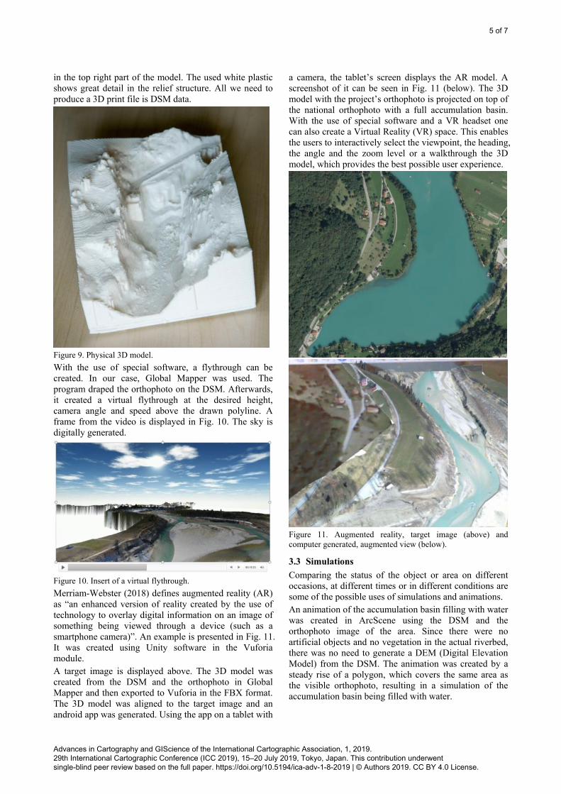
in the top right part of the model. The used white plastic shows great detail in the relief structure. All we need to produce a 3D print file is DSM data.

Figure 9. Physical 3D model.

With the use of special software, a flythrough can be created. In our case, Global Mapper was used. The program draped the orthophoto on the DSM. Afterwards, it created a virtual flythrough at the desired height, camera angle and speed above the drawn polyline. A frame from the video is displayed in Fig. 10. The sky is digitally generated.

Figure 10. Insert of a virtual flythrough.

Merriam-Webster (2018) defines augmented reality (AR) as “an enhanced version of reality created by the use of technology to overlay digital information on an image of something being viewed through a device (such as a smartphone camera)”. An example is presented in Fig. 11. It was created using Unity software in the Vuforia module. A target image is displayed above. The 3D model was created from the DSM and the orthophoto in Global Mapper and then exported to Vuforia in the FBX format. The 3D model was aligned to the target image and an android app was generated. Using the app on a tablet with

a camera, the tablet’s screen displays the AR model. A screenshot of it can be seen in Fig. 11 (below). The 3D model with the project’s orthophoto is projected on top of the national orthophoto with a full accumulation basin. With the use of special software and a VR headset one can also create a Virtual Reality (VR) space. This enables the users to interactively select the viewpoint, the heading, the angle and the zoom level or a walkthrough the 3D model, which provides the best possible user experience.

Figure 11. Augmented reality, target image (above) and computer generated, augmented view (below).

3.3 Simulations

Comparing the status of the object or area on different occasions, at different times or in different conditions are some of the possible uses of simulations and animations. An animation of the accumulation basin filling with water was created in ArcScene using the DSM and the orthophoto image of the area. Since there were no artificial objects and no vegetation in the actual riverbed, there was no need to generate a DEM (Digital Elevation Model) from the DSM. The animation was created by a steady rise of a polygon, which covers the same area as the visible orthophoto, resulting in a simulation of the accumulation basin being filled with water.


6 of 7

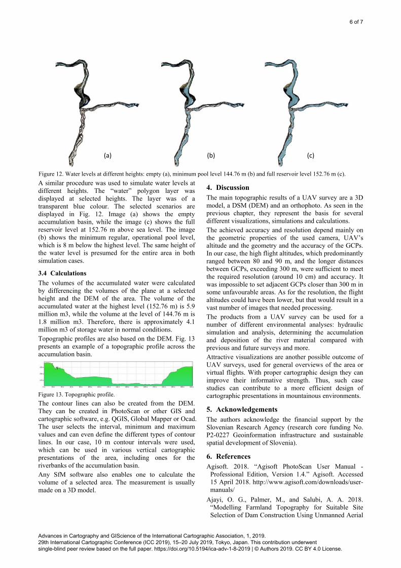
A similar procedure was used to simulate water levels at different heights. The “water” polygon layer was displayed at selected heights. The layer was of a transparent blue colour. The selected scenarios are displayed in Fig. 12. Image (a) shows the empty accumulation basin, while the image (c) shows the full reservoir level at 152.76 m above sea level. The image (b) shows the minimum regular, operational pool level, which is 8 m below the highest level. The same height of the water level is presumed for the entire area in both simulation cases.

3.4 Calculations

The volumes of the accumulated water were calculated by differencing the volumes of the plane at a selected height and the DEM of the area. The volume of the accumulated water at the highest level (152.76 m) is 5.9 million m3, while the volume at the level of 144.76 m is 1.8 million m3. Therefore, there is approximately 4.1 million m3 of storage water in normal conditions. Topographic profiles are also based on the DEM. Fig. 13 presents an example of a topographic profile across the accumulation basin.

Figure 13. Topographic profile.

The contour lines can also be created from the DEM. They can be created in PhotoScan or other GIS and cartographic software, e.g. QGIS, Global Mapper or Ocad. The user selects the interval, minimum and maximum values and can even define the different types of contour lines. In our case, 10 m contour intervals were used, which can be used in various vertical cartographic presentations of the area, including ones for the riverbanks of the accumulation basin. Any SfM software also enables one to calculate the volume of a selected area. The measurement is usually made on a 3D model.

4. Discussion The main topographic results of a UAV survey are a 3D model, a DSM (DEM) and an orthophoto. As seen in the previous chapter, they represent the basis for several different visualizations, simulations and calculations. The achieved accuracy and resolution depend mainly on the geometric properties of the used camera, UAV’s altitude and the geometry and the accuracy of the GCPs. In our case, the high flight altitudes, which predominantly ranged between 80 and 90 m, and the longer distances between GCPs, exceeding 300 m, were sufficient to meet the required resolution (around 10 cm) and accuracy. It was impossible to set adjacent GCPs closer than 300 m in some unfavourable areas. As for the resolution, the flight altitudes could have been lower, but that would result in a vast number of images that needed processing. The products from a UAV survey can be used for a number of different environmental analyses: hydraulic simulation and analysis, determining the accumulation and deposition of the river material compared with previous and future surveys and more. Attractive visualizations are another possible outcome of UAV surveys, used for general overviews of the area or virtual flights. With proper cartographic design they can improve their informative strength. Thus, such case studies can contribute to a more efficient design of cartographic presentations in mountainous environments.

5. Acknowledgements The authors acknowledge the financial support by the Slovenian Research Agency (research core funding No. P2-0227 Geoinformation infrastructure and sustainable spatial development of Slovenia).

6. References Agisoft. 2018. “Agisoft PhotoScan User Manual -

Professional Edition, Version 1.4.” Agisoft. Accessed 15 April 2018. http://www.agisoft.com/downloads/user-manuals/

Ajayi, O. G., Palmer, M., and Salubi, A. A. 2018. “Modelling Farmland Topography for Suitable Site Selection of Dam Construction Using Unmanned Aerial

Figure 12. Water levels at different heights: empty (a), minimum pool level 144.76 m (b) and full reservoir level 152.76 m (c).

(a) (b) (c)


7 of 7

Vehicle (UAV) Photogrammetry.” Remote Sensing Applications: Society and Environment 11 (2018): 220–230. doi: 10.1016/j.rsase.2018.07.007

Clapuyt, F., Vanacker, V., and Van Oost, K. 2016. “Reproducibility of UAV-Based Earth Topography Reconstructions Based on Structure-from-Motion Algorithms.” Geomorphology 260 (2016): 4-15. doi: 10.1016/j.geomorph.2015.05.011

Cook, K. L. 2017. “An Evaluation of the Effectiveness of Low-Cost UAVs and Structure from Motion for Geomorphic Change Detection.” Geomorphology 278 (2017): 195-208. doi: 10.1016/j.geomorph.2016.11.009

Eisenbeiss, Henri. 2009. “UAV Photogrammetry.” PhD diss., ETH Zurich, Switzerland.

Harpha Sea. 2012. “Izmera HE Doblar julij 2012: poročilo o opravljenem delu.”

Hemmelder, S., Marra, W., Markies, H., and De Jong, S. M. 2018. “Monitoring River Morphology & Bank Erosion Using UAV Imagery – A Case Study of the River Buëch, Hautes-Alpes, France.” International Journal of Applied Earth Observation and Geoinformation 73 (2018): 428–437. doi: 10.1016/j.jag.2018.07.016

Hu, G. R., Khoo, H. S., Goh, P. C., and Law, C. L. 2003. “Development and Assessment of GPS Virtual Reference Stations for RTK Positioning.” Journal of Geodesy 77 (2003): 292–302. doi: 10.1007/s00190-003-0327-4

Jorayev, G., Wehr, K., Benito-Calvo, A., Njau, J. and de la Torre, I. 2016. “Imaging and Photogrammetry Models of Olduvai Gorge (Tanzania) by Unmanned Aerial Vehicles: A High-Resolution Ddigital Database for Research and Conservation of Early Stone Age Sites.” Journal of Archaeological Science 75 (2016): 40–56. doi: https://doi.org/10.1016/j.jas.2016.08.002

Mancini, F., Dubbini, M., Gattelli, M., Stecchi, F., Fabbri, S. and Gabbianelli, G. 2013. “Using Unmanned Aerial Vehicles (UAV) for High-Resolution Reconstruction of Topography: The Structure from Motion Approach on Coastal Environments.” Remote Sensing 2013, 5(12): 6880-6898. doi:10.3390/rs5126880

Martínez-Carricondo, P., Agüera-Vega, F., Carvajal-Ramírez, F., Mesas-Carrascosa, F. J., García-Ferrer, A., Pérez-Porras, F. J. 2018. “Assessment of UAV-Photogrammetric Mapping Accuracy Based on Variation of Ground Control Points.” International Journal of Applied Earth Observation and Geoinformation 72 (2018): 1–10. doi: 10.1016/j.jag.2018.05.015

Merriam-Webster. 2018. “Merriam-Webster Dictionary.” Merriam-Webster. Accessed 20 October 2018. https://www.merriam-webster.com/

Retscher, G. 2002. “Accuracy Performance of Virtual Reference Station (VRS) Networks.” Journal of Global Positioning Systems (2002) Vol. 1, No. 1: 40-47.

Soške elektrarne Nova Gorica. 2003. Accessed 20 October 2018. https://www.seng.si/hidroelektrarne/velike-hidroelektrarne/2017060915280084.


Visualizations of the Doblar Accumulation Basin Based on ... · creation of photogrammetry models...

Documents

Transcript of Visualizations of the Doblar Accumulation Basin Based on ... · creation of photogrammetry models...