Pressure-based Solver for Incompressible and Compressible Flows with Cavitation
1
Visualization of three-dimensional incompressible flows by quasi-
two-dimensional divergence-free projections
Alexander Yu. Gelfgat
School of Mechanical Engineering, Faculty of Engineering, Tel-Aviv University, Ramat
Aviv, Tel-Aviv, Israel, 69978, [email protected]
Abstract
A visualization of three-dimensional incompressible flows by divergence-free quasi-two-
dimensional projections of velocity field on three coordinate planes is proposed. It is argued
that such divergence-free projections satisfying all the velocity boundary conditions are
unique for a given velocity field. It is shown that the projected fields and their vector
potentials can be calculated using divergence-free Galerkin bases. Using natural convection
flow in a laterally heated cube as an example, it is shown that the projections proposed allow
for a better understanding of similarities and differences of three-dimensional flows and their
two-dimensional likenesses. An arbitrary choice of projection planes is further illustrated by a
lid-driven flow in a cube, where the lid moves parallel either to a sidewall or a diagonal plane.
Keywords: incompressible flow, flow visualization, Galerkin method, natural convection
benchmark, lid-driven cavity benchmark
2
1. Introduction
With the growth of available computer power, development of numerical methods and
experimental techniques dealing with fully developed three-dimensional flows the importance
of flow visualization becomes obvious. While two-dimensional flows can be easily described
by streamline or vector plots, there is no commonly accepted methodology for representation
of three-dimensional flows on a 2D plot. Streamlines cannot be defined for a general 3D flow.
Other textbook techniques, such as streak lines, trajectories and arrow fields, are widely used
but become unhelpful with increase of flow complicacy. Same can be said about plotting of
isosurfaces and isolines of velocity or vorticity components, which produce beautiful pictures,
however, do not allow one to find out velocity direction at a certain point. Basic and more
advanced recent state-of-the-art visualization techniques are discussed in review papers [1-3]
where reader is referred for the details. Here we develop another visualization technique,
applicable only to incompressible flows, and related to the surface-based techniques discussed
in [2]. Our technique considers projections of 3D velocity field onto coordinate planes and
allows one to compute a set of surfaces to which the projected flow is tangent. Thus, the flow
is visualized in all three sets of coordinate planes (surfaces). The choice of visualization
coordinate system is arbitrary, so that the axes can be directed along "most interesting"
directions, e.g. directions parallel and orthogonal to dominating velocity or vorticity.
The visualization of three-dimensional incompressible flows described below is based on
divergence-free projections of a 3D velocity field on two-dimensional coordinate planes.
Initially, this study was motivated by a need to visualize three-dimensional benchmark flows,
which are direct extensions of well-known two-dimensional benchmarks, e.g., lid-driven
cavity and convection in laterally heated rectangular cavities. Thus, we seek for a
visualization that is capable to show clearly both similarities and differences of flows
considered in 2D and 3D formulations. It seems, however, that the technique proposed can
have significantly wider area of applications.
Consider a given velocity field, which can be a result of computation or experimental
measurement. Note, that modern means of flow measurement, like PIV and PTV, allow one to
measure three velocity components on quite representative grids, which leads to the same
problem of visualization of results. Here we observe that a three-dimensional divergence-free
velocity field can be represented as a superposition of two vector fields that describe the
motion in two sets of coordinate planes, say (x-z) and (y-z), without a need to consider the (x-
3
y) planes. These fields allow for definition of vector potential of velocity, whose two
independent components have properties of two-dimensional stream function. The two parts
of velocity field are tangent to isosurfaces of the vector potential components, which allows
one to visualize the flow in two sets of orthogonal coordinate planes. This approach,
however, does not allow one to preserve the velocity boundary conditions in each of the fields
separately, so that some of the boundary conditions are satisfied only after both fields are
superimposed. The latter is not good for the visualization purposes. We argue further, that it is
possible to define divergence-free projections of the flow on the three sets of coordinate
planes, so that (i) the projections are unique, (ii) each projection is described by a single
component of its vector potential, and (iii) the projection vectors are tangent to isosurfaces of
the corresponding non-zero vector potential component. This allows us to visualize the flow
in three orthogonal sets of coordinate planes. In particular, it helps to understand how the
three-dimensional model flows differ from their two-dimensional likenesses. To calculate the
projections we offer to use divergent-free Galerkin bases, on which the initial flow can be
orthogonally projected.
For a representative example, we choose convection in a laterally heated square cavity
with perfectly thermally insulated horizontal boundaries, and the corresponding three-
dimensional extension, i.e., convection in a laterally heated cube with perfectly insulated
horizontal and spanwise boundaries. The most representative solutions for steady states in
these model flows can be found in [4] for the 2D benchmark, and in [5,6] for the 3D one. In
these benchmarks the pressure , velocity ( ) and temperature are obtained as a
solution of Boussinesq equations
( ) (1)
( ) (2)
(3)
defined in a square or in a cube , with the no-slip boundary
conditions on all the boundaries. The boundaries are isothermal and all the other
boundaries are thermally insulated, which in the dimensionless formulation reads
( ) , ( ) , (
)
, (
)
. (4)
and are the Rayleigh and Prandtl numbers. The reader is referred to the above cited
papers for more details. Here we focus only on visualization of solutions of 3D problem and
comparison with the corresponding 2D flows. All the flows reported below are calculated on
4
1002 and 100
3 stretched finite volume grids, which is accurate enough for present
visualization purposes (for convergence studies see also [7]).
Apparently, the 2D flow ( ) is best visualized by the streamlines, which are
the isolines of the stream function defined as
. In each point the
velocity vector is tangent to a streamline passing through the same point, so that plot of
streamlines and schematic indication of the flow direction is sufficient to visualize a two-
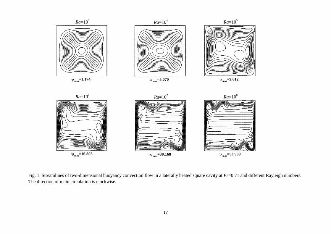
dimensional flow. This is illustrated in Fig. 1, where streamlines of flows calculated for
, and varied from 103 to 10
8 are shown. Note how the streamline patterns
complicate with the increase of Rayleigh number. Our further purpose is to visualize three-
dimensional flows at the same Rayleigh numbers, so that it will be possible to see similarities
and differences of 2D and 3D flows.
2. Preliminary considerations
We consider an incompressible flow in a rectangular box
, satisfying the no-slip conditions on all boundaries. The continuity equation ⁄
⁄ ⁄ makes one velocity component dependent on two others, so that to
describe the velocity field we need two scalar three-dimensional functions, while the third one
can be found via continuity. This observation allows us to decompose the velocity field in the
following way
[
] [
] [
] , ∫
∫
(5)
This decomposition shows that the div-free velocity field can be represented as
superposition of two fields having components only in the (x,z) or (y,z) planes. Moreover, we
can easily define the vector potential of velocity field as
[
] [
∫
∫
] , (6)
Thus, is the vector potential of velocity field , and its two non-zero components have
properties of the stream function:
,
;
,
. (7)
This means, in particular, that vectors of the two components of decomposition (5), i.e.,
( ) and ( ), are tangent to isosurfaces of and , and the vectors are located
5
in the planes (x-z) and (y-z), respectively. Thus, it seems that the isosurfaces of and ,
which can be easily calculated from numerical or experimental (e.g., PIV) data, can be a good
means for visualization of the velocity field. Unfortunately, there is a drawback, which can
make such a visualization meaningless. Namely, only the sum of vectors and ,
calculated via the integrals in (5), vanish at , while each vector separately does not.
Thus, visualization of flow via the decomposition (5) in a straight-forward way will result in
two fields that violate no-penetration boundary conditions at one of the boundaries, which
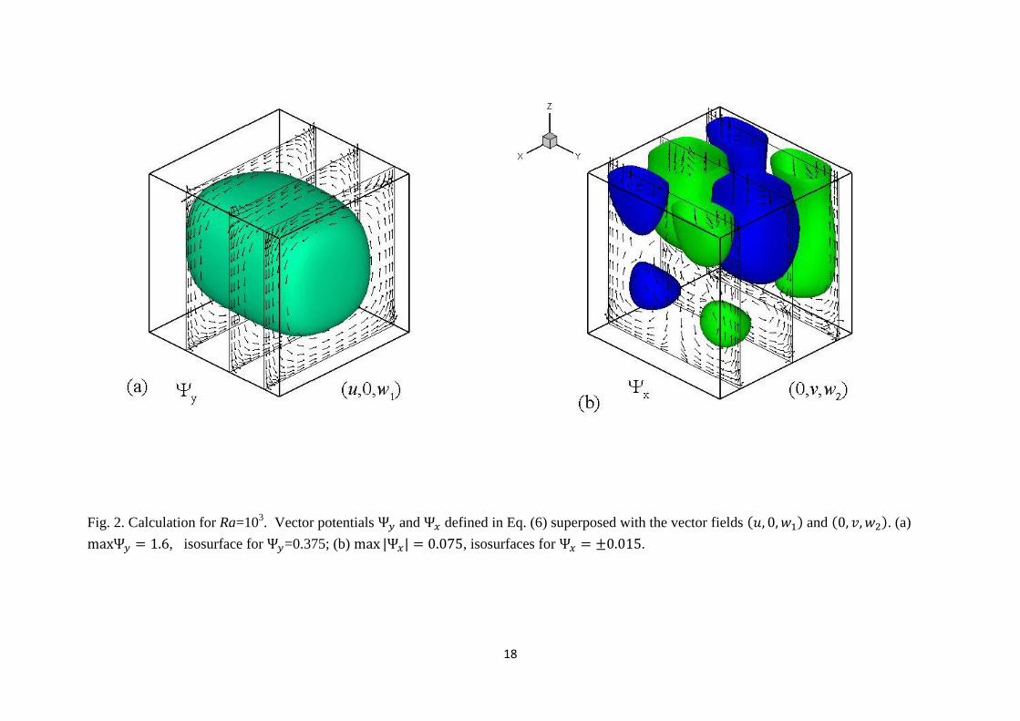
would make the whole result quite meaningless. The latter is illustrated in Fig. 2, where
isosurfaces of the two components of vector potentials are superimposed with the ( )
and ( ) vectors. It is clearly seen that the vector arrows are tangent to the isosurfaces,
however the velocities and do not vanish at the upper boundary. Moreover, the choice
of integration boundaries in (5) is arbitrary, so that the whole decomposition (5) is not unique.
Clearly, one would prefer to visualize unique properties of the flow rather than non-unique
ones.
To define unique flow properties similar to those shown in Fig. 2 we observe that
decomposition (5) can be interpreted as representation of a three-dimensional divergence-free
vector into two divergence free vector fields located in orthogonal coordinate planes, i.e.,
having only two non-zero components. Consider a vector built from only two components of
the initial field, say ( ). It is located in the ( ) planes, satisfies all the
boundary conditions for and , however, is not divergence-free. We can apply the
Helmholtz-Leray decomposition [8] that decomposes this vector into solenoidal and potential
part,
, (8)
As is shown in [8], together with the boundary conditions
, and
(9)
where is a normal to the boundary, the decomposition (8) is unique. For the following, we
consider (8) in the ( ) planes and seek for a decomposition of ( ) in a
( ) plane
( ) , ( ) , ( )
. (10)
We represent the divergent-free two-dimensional vector ( ) as
( )
,
(11)
6
which yields for the z-component of :
(12)
This shows that is an analog of the two-dimensional stream function, so that in each plane
( ) vector is tangent to an isoline of . To satisfy the no-slip boundary
conditions for and , and its normal derivative must vanish on the boundary, which
makes the definition of both and unique. Note, that contrarily to the boundary conditions
(9), to make vector in the decomposition (10) unique and satisfying all the boundary
conditions of , we do not need to define any boundary conditions for the scalar potential .
To conclude, the resulting solenoidal part of vector ( ) (i) is unique, (ii) is
defined by a single non-zero z-component of its vector potential, and (iii) in each
( ) plane vectors of are tangent to the isosurfaces of . Defining same
solenoidal fields for two other sets of coordinate planes we arrive to three quasi-two-
dimensional divergent free projections of the initial velocity field. Each projection is
described by a single scalar three-dimensional function, which, in fact, is a single non-zero
component of the corresponding vector potential.
In the following we use the three above quasi-two-dimensional divergence-free
projections for visualization of convective flow in a laterally heated cube, and offer a way to
calculate them. In particular, to compare a three-dimensional result with the corresponding
two-dimensional one, we need to compare one of the projections. Thus, if the 2D convective
flow was considered in the plane ( ), we compare it with the corresponding projections of
the 3D flow on the ( ) planes, which are tangent to isosurfaces of the non-zero
y-component of the corresponding vector potential.
3. Numerical realization
A direct numerical implementation of the Helmholtz-Leray decomposition to an arbitrary
velocity field is known in CFD as Chorin projection. This procedure is well-known, uses the
boundary conditions (9), but does not preserve all the velocity boundary conditions.
Therefore, it is not applicable for our purposes. Alternatively, we propose orthogonal
projections of the initial velocity field on divergence-free Galerkin bases used previously for
computations of different two-dimensional flows.
Divergence-free basis functions that satisfy all the linear homogeneous boundary
conditions were introduced in [9] for two-dimensional flows and were then extended in
7
[10,11] to three-dimensional cases. To make further numerical process clear we briefly
describe these bases below. The bases are built from shifted Chebyshev polynomials of the 1st
and 2nd
kind, ( ) and ( ), that are defined as
( ) [ ( )], ( ) [( ) ( )]
[ ( )] (13)
and are connected via derivative of ( ) as ( ) ( ). Each of system of
polynomials, either ( ) or ( ), form basis in the space of continuous functions defined
on the interval . It is easy to see that vectors
[
(
) (
)
(
) (
)] (14)
form a divergent-free basis in the space of divergent-free functions defined on a rectangle
. Assume that a two-dimensional problem is defined with two linear
and homogeneous boundary conditions for velocity at each boundary, e.g., the no-slip
conditions. This yields four boundary conditions in either x- or y-direction for the two
velocity components. To satisfy the boundary conditions we extend components of the
vectors (14) into linear superpositions as
[
∑
( ) (
)
∑ (
)
∑
(
)∑
( ) (
)
] (15)
For each a substitution of (15) into the boundary conditions yields four linear homogeneous
equations for five coefficients Fixing , allows one to define all the
other coefficients, whose dependence on and can be derived analytically. The coefficients
are evaluated in the same way. Expressions for these coefficients for the no-slip boundary
conditions can be found in [9,11]. Since the basis functions are divergence-free in the
plane ( ), ( )
⁄ (
)
⁄ , and satisfy the non-penetration conditions
through all the boundaries and , they are orthogonal to every two-
dimensional potential vector field, i.e.,
∫ ∫
∫ ∫ (
)
, (16)
which is an important point for further evaluations.
8
For extension of the two-dimensional basis to the three dimensional case we recall that
for divergence-free vector field we have to define independent three-dimensional bases for
two components only. Representing the flow in the form (6) and using the same idea as in the
two-dimensional basis (15) we arrive to a set of three-dimensional basis functions formed
from two following subsets
( )
( )
[
∑
( ) (
)
∑ (
)
∑ (
)
∑
(
)∑ (
)
∑
( ) (
)
]
(17)
( )( )
[
∑ (
)
∑
( ) (
)
∑ (
)
∑ (
)
∑ (
)
∑
( ) (
)
]
(18)
Where coefficients , , , , , are defined from the boundary conditions. Their
expressions for no-slip boundary conditions are given in [11]. The velocity field is
approximated as a truncated series
( ) ( ) ( ) ∑ ∑ ∑ ( )
, ( ) ∑ ∑ ∑
( )
(19)
Here one must be cautious with the boundary conditions in z-direction since, as it was
explained above, the two parts of representation (6) satisfy the boundary condition for at
only as a sum. Therefore we must exclude this condition from definition of basis
functions (17) and (18) and set . The corresponding boundary condition should
be included in the resulting system of equations for and as an additional algebraic
constraint. Note that this fact was overlooked in [10] that could lead to missing of some
important three-dimensional Rayleigh-Bénard modes. On the other hand, comparison of 3D
basis functions (16) and (17) with the 2D ones (15) shows that with all the boundary
conditions included, the functions ( )
( ) and ( )( ) form the complete two-
dimensional bases in the ( ) and ( ) planes, respectively. The
coefficients and are used to satisfy the boundary conditions in the third direction. For
the basis in the ( ) planes we add

9
( )( )
[
∑
( ) (
)
∑ (
)
∑ (
)
∑ (
)
∑
( ) (
)
∑ (
)
]
(20)
Now, we define an inner product as
⟨ ⟩ ∫
(21)
and compute projections of the initial velocity vector on each of the three basis systems
separately. Together with the vectors ( ) and ( )defined in Eq. (19) we obtain also vector
( ) ∑ ∑ ∑ ( )
(22)
Since the basis vectors ( )
( )
and ( )
satisfy all the boundary conditions and are
divergence-free not only in the 3D space, but also into the corresponding coordinate planes,
the potential parts of projections on these planes are excluded by (16), and resulting vectors
( ) ( ) ( ) satisfy the boundary conditions and are divergence free in the planes they are
located. Therefore, they approximate the quasi-two-dimensional divergent-free projection
vectors we are looking for. Note, however, that the superposition ( ) ( ) ( ) does not
approximate the initial vector . To complete the visualization we have to derive the
corresponding approximation of vector potentials. The vector potential of each of
( ) ( ) ( ) has only one non-zero component, as is defined below
( ) ( ) ( ) ( ( )
) ( )
∑ ∑ ∑ ( )
,
( ) ( ) ( ) ( ( )
) ( )
∑ ∑ ∑ ( )
, (23)
( ) ( ) ( ) ( ( )
) ( )
∑ ∑ ∑ ( )
where
( )( ) ∑ (
)
∑
( ) (
)
∑
( ) (
)
( )
( ) ∑
( ) (
)
∑ (
)
∑
( ) (
)
(24)
( )( ) ∑
( ) (
)
∑
( ) (
)
∑ (
)
10
As stated above, the vectors ( ) ( ) ( ) are tangent to the isosurfaces of ( )
, ( )
and
( )
, respectively.
4. Visualization results
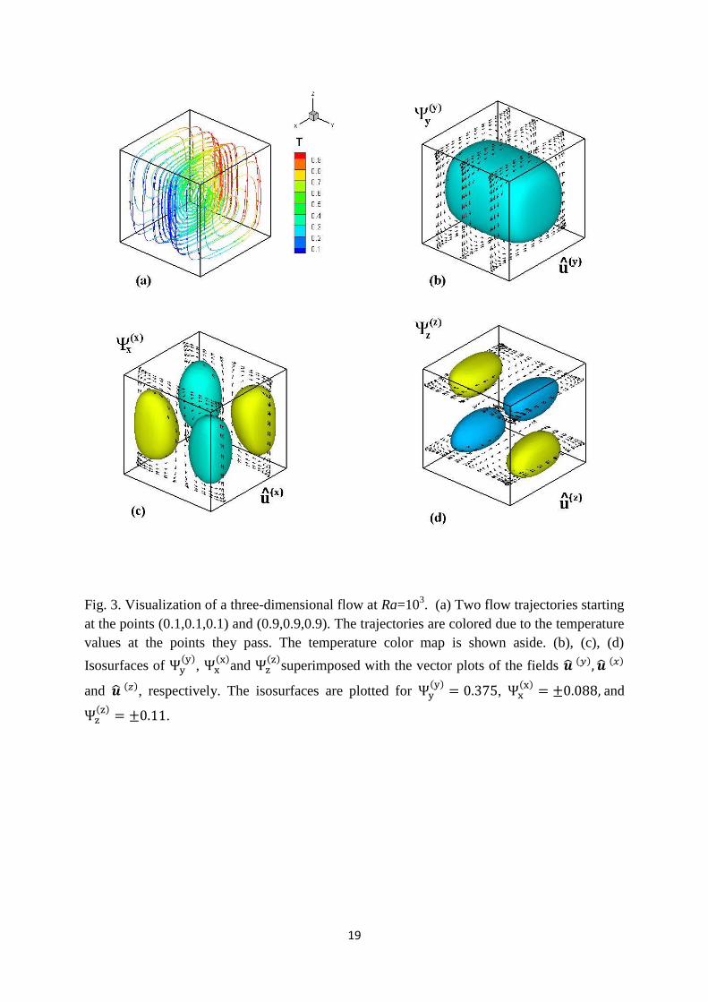
We start from the flow at that has the simplest pattern (Fig. 3). Figure 3a
shows two trajectories starting in points (0.1,0.1,0.1) and (0.9,0.9,0.9). The trajectories are
colored according to the values of temperature they pass, so that it is clearly seen that the fluid
rises near the hot wall and descends near the cold one. Looking only at the trajectories, one
can mistakenly conclude that convective circulation weakens toward the center plane .
Frames 3b-3d show that this impression is misleading. In these frames we plot three vector
potentials defined in Eqs. (23), together with the divergent-free velocity projections (shown
by arrows) on the corresponding coordinate planes. First, it is clearly seen that the projection
vectors are tangent to the isolines of the vector potentials. Then we observe that projections
on the planes (Fig. 3b) represent the simple convective two-dimensional
circulation shown in Fig. 1a. Contrarily to the impression of Fig. 3a, the circulations in ( )
are almost y-independent near the center plane and steeply decay near the boundaries
and . The three-dimensional effects are rather clearly seen from the two
remaining frames. The flow contains two pairs of diagonally symmetric rolls in the ( )
planes (Fig. 3c), and two other diagonally symmetric rolls in the ( ) planes (Fig. 3d).
Motion along these rolls deforms trajectories shown in Fig. 3a.
It is intuitively clear that the motion in the frames of Fig. 3c and 3d is noticeably weaker
than that in Fig. 3b. For the 2D flows the integral intensity of convective circulation can be
estimated by the maximal value of the stream function. Similarly, here we can estimate the
intensity of motion in two-dimensional planes by maximal values of the corresponding vector
potential. Since these values can be used also for comparison of results obtained by different
methods we report all of them, together with their locations, in Table 1. As expected, we
observe that at the maximal value of ( )
is larger than that of two other potentials
in almost an order of magnitude. With the increase of Rayleigh number the ratio of maximal
values of ( )
, ( )
and ( )
grows reaching approximately one half at , which
indicates on the growing importance of motion in the third direction.
11
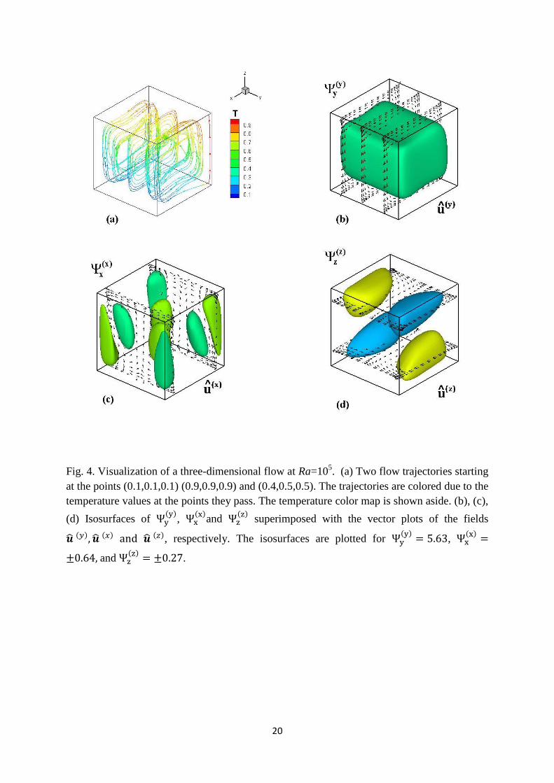
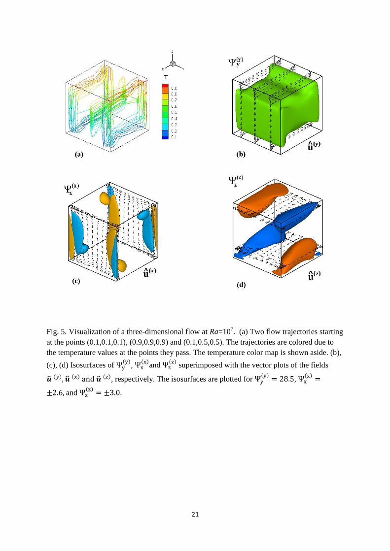
Figures 4-6 illustrate flows at , 107 and 10
8, respectively, in the same way as in
Fig. 3. It is seen that the isosurfaces of ( )
resemble the shapes of two-dimensional
streamlines (Fig. 1) rather closely. At the same time we see that the “three-dimensional
additions” to the flow, represented by ( )
and ( )
, remain located near the no-slip
boundaries and are weak in the central region of the cavity. This means, in particular, that
spanwise directed motion in the midplane is weak, which justifies use of two-
dimensional model for description of the main convective circulation.
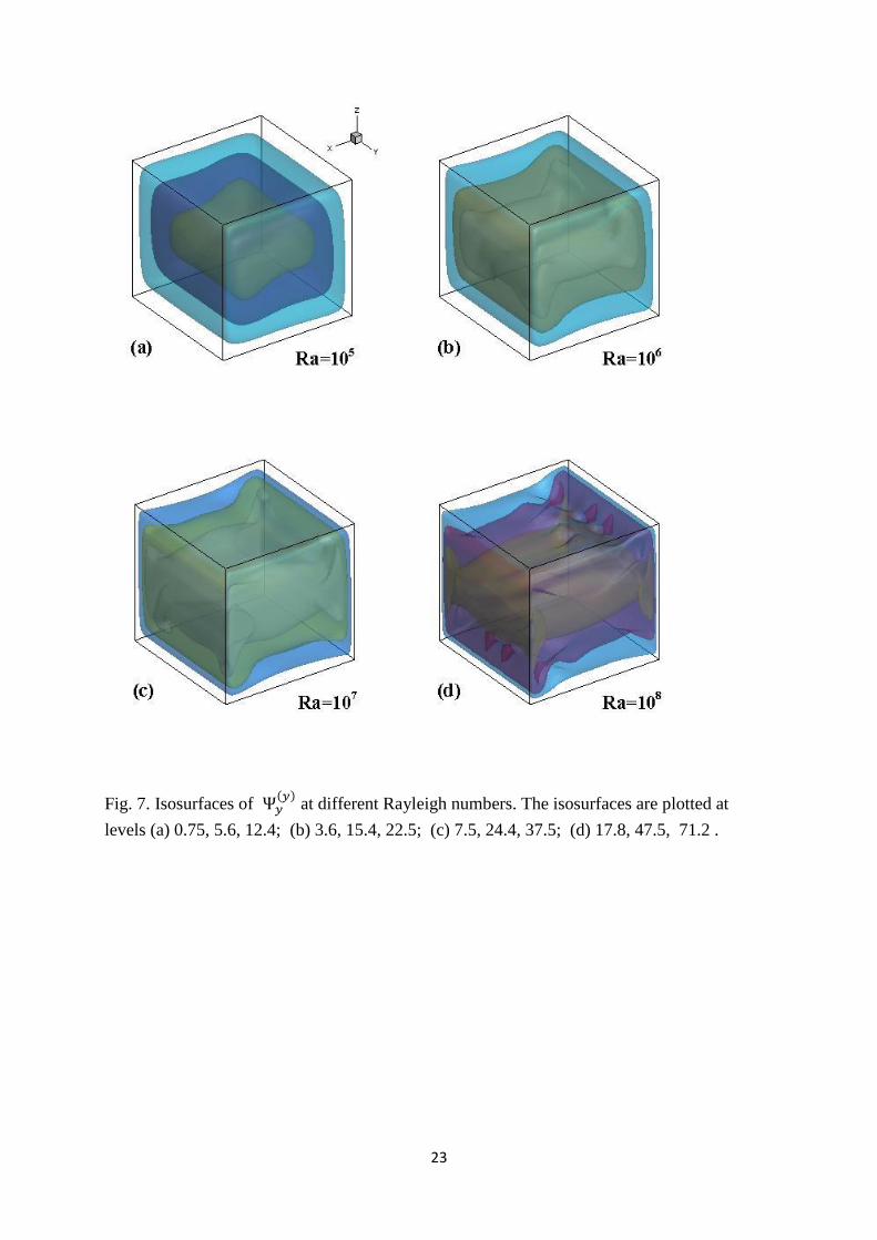
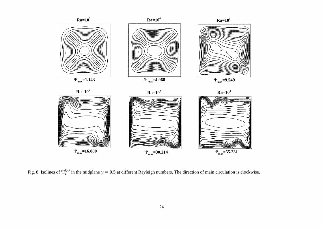
To show how the isosurfaces of ( )
represent patterns of two-dimensional flow we show
their several isosurfaces in Fig. 7 and isolines in the center plane in Fig. 8. The
isosurfaces of ( )
in Fig. 7 shows pattern of the main convective circulation in the (
) planes. The isolines in Fig. 8 can be directly compared with the streamlines shown
in Fig. 1. This comparison should be accompanied with the comparison of the maximal values
of the stream functions of Fig. 1 and the maximal values of ( )
, all shown in the figures. We
observe that the patterns in Figs. 1 and 8 remain similar, however the similarity diminishes
with the increase of Ra. The maximal values of ( )
for are smaller than that of the
stream function, which can be easily explained by additional friction losses due to the
spanwise boundaries added to the three-dimensional formulation. At we observe
that together with the deviation of the isolines pattern from the 2D one, the maximal values of
( )
become larger than those of the two-dimensional stream function. Ensuring, that this is
not an effect of truncation in the sums (23), we explain this by strong three-dimensional
effects, in which motion along the y-axis start to affect the motion in the ( )
planes.
As an example of arbitrary choice of projection planes we consider another well-known
benchmark problem of flow in a lid-driven cubic cavity. We consider it in two different
formulations: a classical configuration where the lid moves parallel to a side wall, and a
modified configuration with the lid moving along the diagonal of the upper boundary [12].
Obviously, three-dimensional effects are significantly stronger in the second case. Both flows
are depicted in Figs. 9 and 10 in the same way as convective flows were represented above.
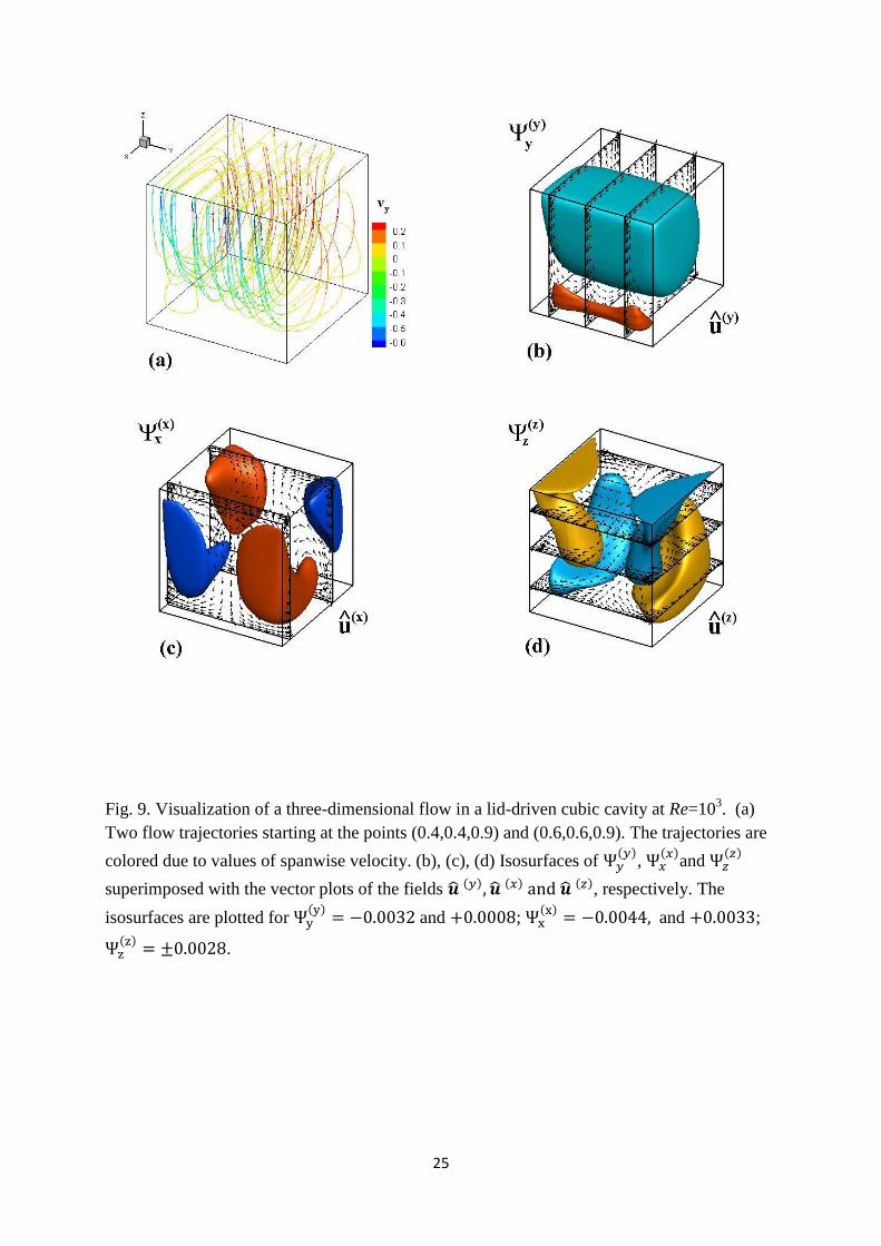
Comparing the flow pattern shown in Fig. 9, one can see clear similarities with the well-
known two-dimensional flow in a lid-driven cavity. The main vortex and reverse recirculation
in the lower corner are clearly seen in Fig, 9b. Figures 9c and 9d show additional three-
dimensional recirculations in the ( ) and ( ) planes. The same
12
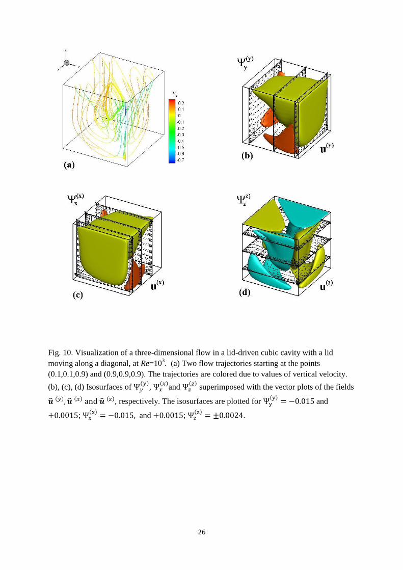
representation of the second configuration in Fig. 10 exhibits similar patterns of ( )
and
( )
together with the similar patterns of corresponding projection vectors. This is an obvious
consequence of the problem configuration, where main motion is located in the diagonal
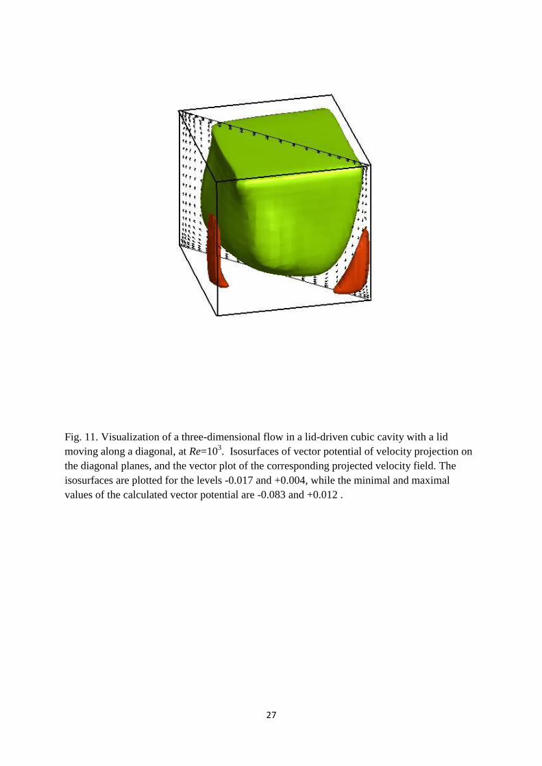
plane and the planes parallel to it. To illustrate motion in these planes we project the flow on
planes orthogonal to the diagonal plane (or parallel to the second diagonal plane). The result
is shown in Fig. 11. The isosurfaces belong to the corresponding vector potential, so that the
divergence-free projection of velocity on the diagonal and parallel planes is tangent to these
and other isosurfaces. Arrows in the diagonal plane depict this projection and illustrate the
main vortex, as well as small recirculation vortices in lower corners. It is seen that the arrows
are tangent to both isosurfaces.
5. Conclusions
We proposed to visualize three-dimensional incompressible flows by divergence-free
projections of velocity field on three coordinate planes. We presented the arguments showing
that such a representation allows, in particular, for a better understanding of similarities and
differences between three-dimensional benchmark flow models and their two-dimensional
counter parts. We argued also that the choice of projection planes is arbitrary, so that they can
be fitted to the flow pattern.
To approximate the divergence-free projections numerically we calculated orthogonal
projections on divergence-free Galerkin velocity bases. Obviously, there are other ways of
doing that, among which we can mention inverse of the Stokes operator discussed in [13]. We
believe also that the proposed method of visualization is suitable for a significantly wider
class of incompressible flows, and can be applied not only to numerical, but also to
experimental data.
Acknowledgement
This work was supported by the LinkSCEEM-2 project, funded by the European Commission
under the 7th Framework Program through Capacities Research Infrastructure, INFRA-2010-
1.2.3 Virtual Research Communities, Combination of Collaborative Project and Coordination
and Support Actions (CP-CSA) under grant agreement no RI-261600.
13
References
1. McLaughlin T., Laramee R.S., Peikert R., Post F.H., Chen M., Over two decades of
integration-based, geometric flow visualization. Computer Graphics Forum, 2010; 29:
1807-1829.
2. Edmunds M., Laramee R.S., Chen G., Max N., Zhang E., Ware C., Surface-based flow
visualization, Computers & Graphics, 2012; 36: 974-990.
3. Etien T., Nguyen H., Kirby R.M., Siva C.T., "Flow visualization" juxtaposed with
"visualization of flow": synergistic opportunities between two communities, Proc. 51st
AIAA Aerosp. Sci. Meet. New Horiz. Forum Aerosp. Exp., 2013; 1-13.
4. Le Quéré P., Accurate solutions to the square thermally driven cavity at high Rayleigh
number. Computers and Fluids 1991; 20: 29–41.
5. Tric E., Labrosse G., Betrouni M., A first incursion into the 3D structure of natural
convection of air in a differentially heated cavity, from accurate numerical solutions. Int J
Heat Mass Transf 1999; 43: 4043-4056.
6. Wakashima S, Saitoh TS. Benchmark solutions for natural convection in a cubic cavity
using the high-order time-space method. Int J Heat Mass Transf 2004; 47: 853–64.
7. Gelfgat A. Yu. Stability of convective flows in cavities: solution of benchmark
problems by a low-order finite volume method. Int J Numer Meths Fluids 2007; 53:
485-506.
8. Foias C., Manley O., Rosa R., Temam R. Navier-Stokes Equations and Turbulence.
Cambridge Univ. Press, 2001.
9. Gelfgat A.Yu. and Tanasawa I. Numerical analysis of oscillatory instability of
buoyancy convection with the Galerkin spectral method. Numer Heat Transf. Pt A
1994; 25(6): 627-648.
10. Gelfgat A. Yu. Different modes of Rayleigh-Bénard instability in two- and three-
dimensional rectangular enclosures. J Comput Phys 1999; 156: 300-324.
11. Gelfgat A. Yu. Two- and three-dimensional instabilities of confined flows: numerical
study by a global Galerkin method. Comput Fluid Dyn J 2001; 9: 437-448.
12. Feldman Yu., Gelfgat A. Yu. From multi- to single-grid CFD on massively parallel
computers: numerical experiments on lid-driven flow in a cube using pressure-velocity
coupled formulation. Computers & Fluids 2011; 46: 218-223.
13. Vitoshkin H., Gelfgat A. Yu. On direct inverse of Stokes, Helmholtz and Laplacian
operators in view of time-stepper-based Newton and Arnoldi solvers in incompressible
CFD. Communications in Computational Physics 2013; 14: 1103-1119.
14
Figure captions
Fig. 1. Streamlines of two-dimensional buoyancy convection flow in a laterally heated square
cavity at Pr=0.71 and different Rayleigh numbers. The direction of main circulation is
clockwise.
Fig. 2. Calculation for Ra=103. Vector potentials and defined in Eq. (6) superposed
with the vector fields ( ) and ( ). . (a) , isosurface for =0.375;
(b) , isosurfaces for .
Fig. 3. Visualization of a three-dimensional flow at Ra=103. (a) Two flow trajectories starting
at the points (0.1,0.1,0.1) and (0.9,0.9,0.9). The trajectories are colored due to the temperature
values at the points they pass. The temperature color map is shown aside. (b), (c), (d)
Isosurfaces of ( )
, ( )
and ( )
superimposed with the vector plots of the fields ( ) ( )
and ( ), respectively. The isosurfaces are plotted for ( )
, ( )
and
( ) .
Fig. 4. Visualization of a three-dimensional flow at Ra=105. (a) Two flow trajectories starting
at the points (0.1,0.1,0.1) (0.9,0.9,0.9) and (0.4,0.5,0.5). The trajectories are colored due to the
temperature values at the points they pass. The temperature color map is shown aside. (b), (c),
(d) Isosurfaces of ( )
, ( )
and ( )
superimposed with the vector plots of the fields
( ) ( ) and ( ), respectively. The isosurfaces are plotted for ( )
, ( )
and ( ) .
Fig. 5. Visualization of a three-dimensional flow at Ra=107. (a) Two flow trajectories starting
at the points (0.1,0.1,0.1), (0.9,0.9,0.9) and (0.1,0.5,0.5). The trajectories are colored due to
the temperature values at the points they pass. The temperature color map is shown aside. (b),
(c), (d) Isosurfaces of ( )
, ( )
and ( )
superimposed with the vector plots of the fields
( ) ( ) and ( ), respectively. The isosurfaces are plotted for ( )
, ( )
and ( )
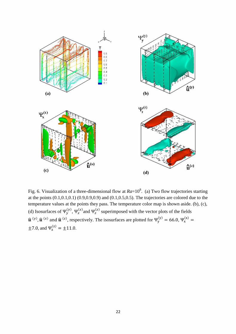
Fig. 6. Visualization of a three-dimensional flow at Ra=108. (a) Two flow trajectories starting
at the points (0.1,0.1,0.1) (0.9,0.9,0.9) and (0.1,0.5,0.5). The trajectories are colored due to the
temperature values at the points they pass. The temperature color map is shown aside. (b), (c),
(d) Isosurfaces of ( )
, ( )
and ( )
superimposed with the vector plots of the fields
( ) ( ) and ( ), respectively. The isosurfaces are plotted for ( )
, ( )
and ( ) .
Fig. 7. Isosurfaces of ( )
at different Rayleigh numbers. The isosurfaces are plotted at
levels (a) 0.75, 5.6, 12.4; (b) 3.6, 15.4, 22.5; (c) 7.5, 24.4, 37.5; (d) 17.8, 47.5, 71.2 .
15
Fig. 8. Isolines of ( )
in the midplane at different Rayleigh numbers. The direction
of main circulation is clockwise.
Fig. 9. Visualization of a three-dimensional flow in a lid-driven cubic cavity at Re=103. (a)
Two flow trajectories starting at the points (0.4,0.4,0.9) and (0.6,0.6,0.9). The trajectories are
colored due to values of spanwise velocity. (b), (c), (d) Isosurfaces of ( )
, ( )
and ( )
superimposed with the vector plots of the fields ( ) ( ) and ( ), respectively. The
isosurfaces are plotted for ( )
and ; ( )
and ;
( ) .
Fig. 10. Visualization of a three-dimensional flow in a lid-driven cubic cavity with a lid
moving along a diagonal, at Re=103. (a) Two flow trajectories starting at the points
(0.1,0.1,0.9) and (0.9,0.9,0.9). The trajectories are colored due to values of vertical velocity.
(b), (c), (d) Isosurfaces of ( )
, ( )
and ( )
superimposed with the vector plots of the fields
( ) ( ) and ( ), respectively. The isosurfaces are plotted for ( )
and ;
( )
and ; ( ) .
Fig. 11. Visualization of a three-dimensional flow in a lid-driven cubic cavity with a lid
moving along a diagonal, at Re=103. Isosurfaces of vector potential of velocity projection on
the diagonal planes, and the vector plot of the corresponding projected velocity field. The
isosurfaces are plotted for the levels -0.017 and +0.004, while the minimal and maximal
values of the calculated vector potential are -0.083 and +0.012 .
16
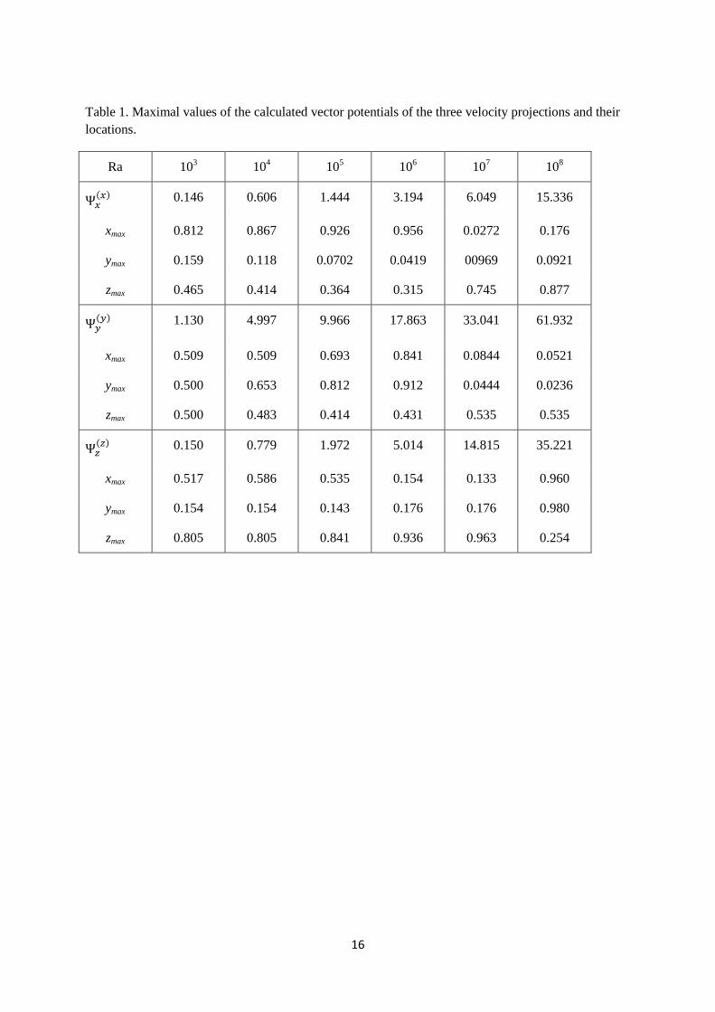
Table 1. Maximal values of the calculated vector potentials of the three velocity projections and their
locations.
Ra 103 10
4 10
5 10
6 10
7 10
8
( )
0.146 0.606 1.444 3.194 6.049 15.336
xmax 0.812 0.867 0.926 0.956 0.0272 0.176
ymax 0.159 0.118 0.0702 0.0419 00969 0.0921
zmax 0.465 0.414 0.364 0.315 0.745 0.877
( )
1.130 4.997 9.966 17.863 33.041 61.932
xmax 0.509 0.509 0.693 0.841 0.0844 0.0521
ymax 0.500 0.653 0.812 0.912 0.0444 0.0236
zmax 0.500 0.483 0.414 0.431 0.535 0.535
( )
0.150 0.779 1.972 5.014 14.815 35.221
xmax 0.517 0.586 0.535 0.154 0.133 0.960
ymax 0.154 0.154 0.143 0.176 0.176 0.980
zmax 0.805 0.805 0.841 0.936 0.963 0.254
17
Ra=103
max
=1.174
Ra=104
max
=5.070
Ra=105
max
=9.612
Ra=106
max
=16.803
Ra=107
max
=30.168
Ra=108
max
=53.999
Fig. 1. Streamlines of two-dimensional buoyancy convection flow in a laterally heated square cavity at Pr=0.71 and different Rayleigh numbers.
The direction of main circulation is clockwise.
18
Fig. 2. Calculation for Ra=103. Vector potentials and defined in Eq. (6) superposed with the vector fields ( ) and ( ). (a)
, isosurface for =0.375; (b) , isosurfaces for .
19
Fig. 3. Visualization of a three-dimensional flow at Ra=103. (a) Two flow trajectories starting
at the points (0.1,0.1,0.1) and (0.9,0.9,0.9). The trajectories are colored due to the temperature
values at the points they pass. The temperature color map is shown aside. (b), (c), (d)
Isosurfaces of ( )
, ( )
and ( )
superimposed with the vector plots of the fields ( ) ( )
and ( ), respectively. The isosurfaces are plotted for ( )
, ( )
and
( ) .
20
Fig. 4. Visualization of a three-dimensional flow at Ra=105. (a) Two flow trajectories starting
at the points (0.1,0.1,0.1) (0.9,0.9,0.9) and (0.4,0.5,0.5). The trajectories are colored due to the
temperature values at the points they pass. The temperature color map is shown aside. (b), (c),
(d) Isosurfaces of ( )
, ( )
and ( )
superimposed with the vector plots of the fields
( ) ( ) and ( ), respectively. The isosurfaces are plotted for ( )
, ( )
and ( ) .
21
Fig. 5. Visualization of a three-dimensional flow at Ra=107. (a) Two flow trajectories starting
at the points (0.1,0.1,0.1), (0.9,0.9,0.9) and (0.1,0.5,0.5). The trajectories are colored due to
the temperature values at the points they pass. The temperature color map is shown aside. (b),
(c), (d) Isosurfaces of ( )
, ( )
and ( )
superimposed with the vector plots of the fields
( ) ( ) and ( ), respectively. The isosurfaces are plotted for ( )
, ( )
and ( ) .
22
Fig. 6. Visualization of a three-dimensional flow at Ra=108. (a) Two flow trajectories starting
at the points (0.1,0.1,0.1) (0.9,0.9,0.9) and (0.1,0.5,0.5). The trajectories are colored due to the
temperature values at the points they pass. The temperature color map is shown aside. (b), (c),
(d) Isosurfaces of ( )
, ( )
and ( )
superimposed with the vector plots of the fields
( ) ( ) and ( ), respectively. The isosurfaces are plotted for ( )
, ( )
and ( ) .
23
Fig. 7. Isosurfaces of ( )
at different Rayleigh numbers. The isosurfaces are plotted at
levels (a) 0.75, 5.6, 12.4; (b) 3.6, 15.4, 22.5; (c) 7.5, 24.4, 37.5; (d) 17.8, 47.5, 71.2 .
24
Ra=103
max
=1.143
Ra=104
max
=4.968
Ra=105
max
=9.549
Ra=106
max
=16.800
Ra=107
max
=30.214
Ra=108
max
=55.231
Fig. 8. Isolines of ( )
in the midplane at different Rayleigh numbers. The direction of main circulation is clockwise.
25
Fig. 9. Visualization of a three-dimensional flow in a lid-driven cubic cavity at Re=103. (a)
Two flow trajectories starting at the points (0.4,0.4,0.9) and (0.6,0.6,0.9). The trajectories are
colored due to values of spanwise velocity. (b), (c), (d) Isosurfaces of ( )
, ( )
and ( )
superimposed with the vector plots of the fields ( ) ( ) and ( ), respectively. The
isosurfaces are plotted for ( )
and ; ( )
and ;
( ) .
26
Fig. 10. Visualization of a three-dimensional flow in a lid-driven cubic cavity with a lid
moving along a diagonal, at Re=103. (a) Two flow trajectories starting at the points
(0.1,0.1,0.9) and (0.9,0.9,0.9). The trajectories are colored due to values of vertical velocity.
(b), (c), (d) Isosurfaces of ( )
, ( )
and ( )
superimposed with the vector plots of the fields
( ) ( ) and ( ), respectively. The isosurfaces are plotted for ( )
and
; ( )
and ; ( ) .
27
Fig. 11. Visualization of a three-dimensional flow in a lid-driven cubic cavity with a lid
moving along a diagonal, at Re=103. Isosurfaces of vector potential of velocity projection on
the diagonal planes, and the vector plot of the corresponding projected velocity field. The
isosurfaces are plotted for the levels -0.017 and +0.004, while the minimal and maximal
values of the calculated vector potential are -0.083 and +0.012 .