VISUALIZATION OF HYPERSPECTRAL IMAGES

ROBERTO BONCE & MINDY SCHOCKLINGiMagine REU Montclair State University

Presentation Overview

Hyperspectral Images Wavelet Transform MATLAB code and results Conclusions References

Problem Statement

How can hyperspectral data be manipulated to enable visualization of the important information they contain?

What are hyperspectral images?

Most images contain only data in the visible spectrum

Hyperspectral images contain data from many, closely spaced wavelengths

Our camera records data from 400nm to 900nm

Hyperspectral cont.

Hyperspectral images can be thought of as being stacked on top of each other, creating an image cube

A pixel vector can be used to distinguish one material from another

Pictures

Wavelets: “small waves”

Decay as distance from the center increases

Have some sense of periodicity

Can perform local analysis unlike Fourier

Wavelet Analysis and Reconstruction

Original signal is sent through high and low pass filters

Approximation: low frequency, general shape Detail: high frequency, noise Reconstruction involves filtering and

upsampling

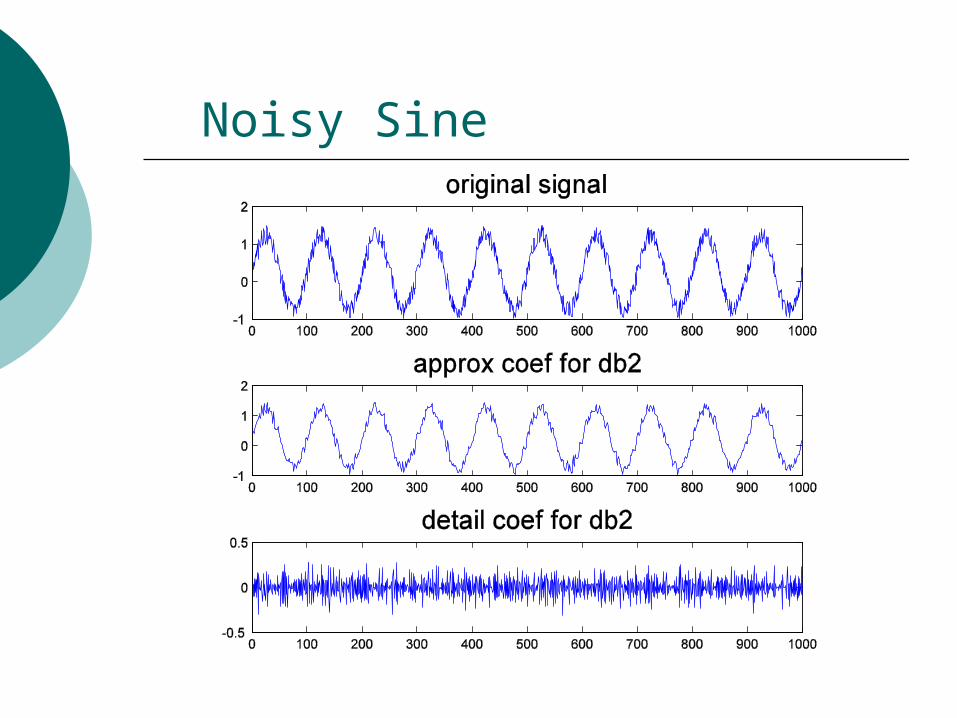
Noisy Sine

The Project

Analyzing hyperspectral signatures for image analysis can be very computationally expensive

One approach to the problem is to select a subset of the images and apply a weighting scheme to generate a useful image

Project Cont.

The plant to the right contains both real and artificial leaves

Goal: distinguish between real and artificial leaves

Last Year (2007)

Focus bands were chosen Applied a weighting scheme

To give near infrared data more importance because the visual data is too similar

An RGB composite image is created

Last Year

Composite image to the right

They used the distance series

Preliminary results

Tried weighting, wavelet transform, different focus bands.

Results were somewhat disappointing

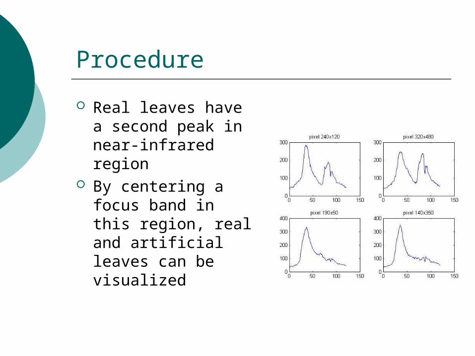
Procedure

Real leaves have a second peak in near-infrared region

By centering a focus band in this region, real and artificial leaves can be visualized

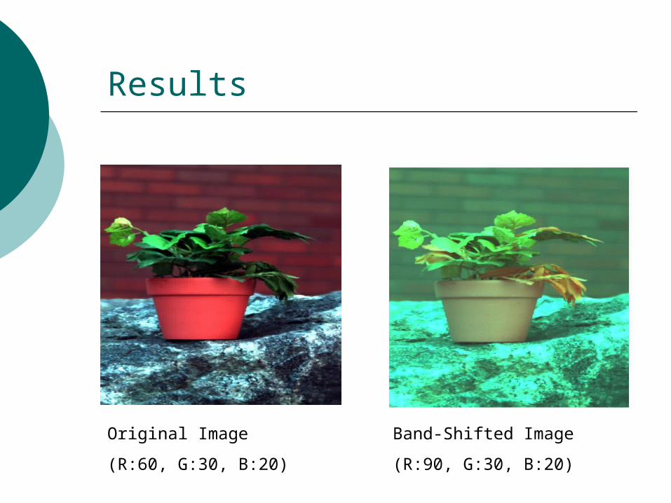
Results

Original Image

(R:60, G:30, B:20)

Band-Shifted Image

(R:90, G:30, B:20)

Gaussian Weighting

Similar to last approach Choose 3 focus bands Use Gaussian curve to do a

weighted average of nearby bands Create RGB composite image Results are heavily dependent on

what focus bands are chosen

Gaussian Weighting

Figure 9 Weighted average of 3 images near bands 70, 80, and 90. The green leaves are real, the purple leaves are fake

Gaussian Weighting

Figure 10 weighting using 6 images near bands 20, 30, and 40

New Approach

Instead of using 2D images from the cube, use 1D pixel vectors

Idea #1 Choose 3 spectral vectors Do some sort of average Use bands corresponding to the

maximum or minimum points to do an RGB composite

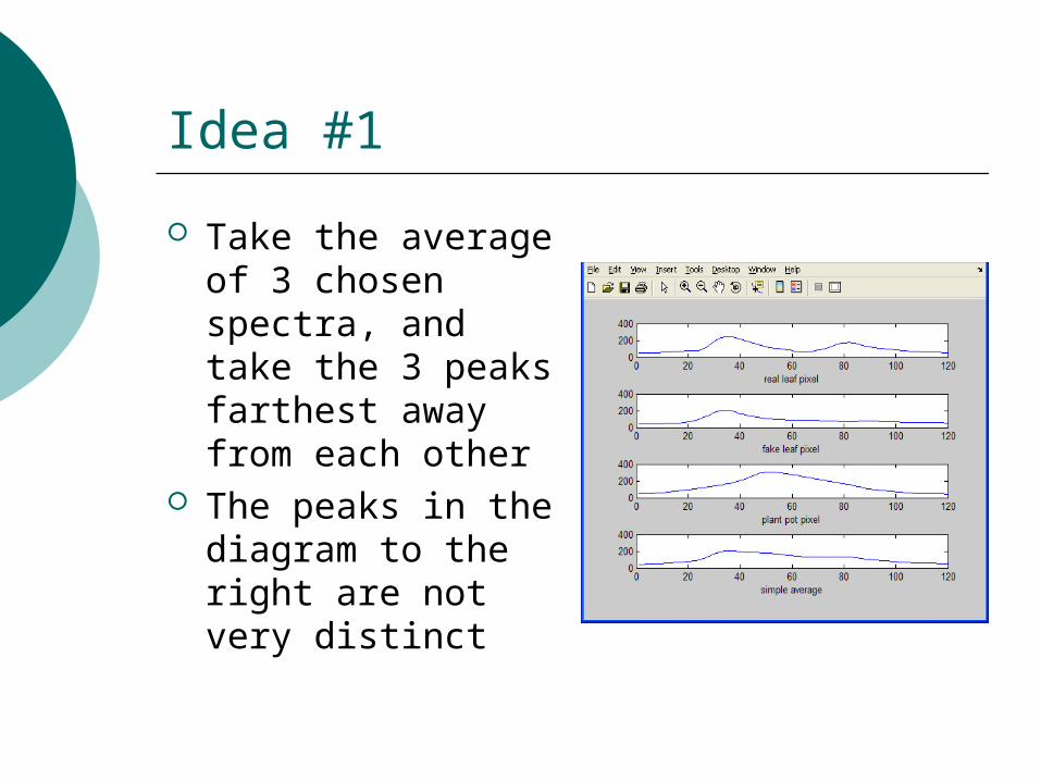
Idea #1

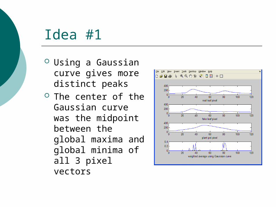
Take the average of 3 chosen spectra, and take the 3 peaks farthest away from each other

The peaks in the diagram to the right are not very distinct

Idea #1

Using a Gaussian curve gives more distinct peaks

The center of the Gaussian curve was the midpoint between the global maxima and global minima of all 3 pixel vectors

Idea #1 results

Figure 13 real leaf, fake leaf, and pot pixel vectors chosen. Using local maxima

Idea #1 results

Figure 15 Using the furthest away regional minima, rather than regional minima.

Idea #1 results

Figure 16 pixel vector chosen from brick wall, plant pot, and dark rock. Used local maxima

Idea #1 results

Figure 17 pixel vector chosen from brick wall, plant pot, and dark rock. Used local minima

Idea #1 results

Figure 18 pixel chosen were brick, fake leaf, and rock. Used local minima.

Idea #1 results

Figure 19 pixel chosen were brick, fake leaf, and rock. Used local maxima.

New Approach

Idea #2 Choose pixels of interest Perform wavelet decomposition Identify coefficient positions with

maxima Perform decomposition on all pixels Use chosen coefficients to produce a

color image

Idea #2 Results

Chose 1 pixel within a real leaf and 1 pixel in brick wall for “pixels of interest”

Maxima identified for use as color values R:44 G:20 B:28

Idea #2 Results

Top: results using wavelet coefficients

Bottom: results using bands directly

Conclusions

Using wavelet coefficients could provide a superior means for visualization in some cases

Computationally expensive More precise method for selection of

pixels/peaks is needed

References:

http://www.microimages.com/getstart/pdf/hyprspec.pdf

Images from http://www.wikipedia.org/

MATLAB help