Visualising Uncertainty in Spatially-Referenced Attribute Data using Hierarchical Spatial Data Structures

J.D. Kardos, A. Moore and G.L. Benwell

Department of Information Science, University of Otago,

Dunedin, New Zealand. Telephone: +64 3 479 8301

FAX: +64 3 479 8311 Email: jkardos@infoscience.otago.ac.nz

Abstract This paper presents the use of hierarchical spatial data structures to visualise uncertainty in spatial information. This is demonstrated using spatial data from the New Zealand 2001 Census. Current visualisation of uncertainty techniques are evaluated, and a new method is proposed. This paper assesses the value of hierarchical tree structures as a geovisualisation of attribute uncertainty technique. Two such structures will be compared: the region quadtree and the Hexagonal or Rhombus (HoR) quadtree, both variable resolution structures. An area where attribute data is uncertain will show less resolution through the data structure than an area that is not, exemplifying a metaphor of detail. The major question is: can an uncertainty value be effectively communicated using tree structures when simultaneously displayed with the attribute information? Principles of possible implementations are presented through outlining a demonstration program, TRUST (The Representation of Uncertainty using Scale-unspecific Tessellations).

1. Introduction Spatial and attribute information have an inherent associated uncertainty that may need to be expressed to a potential user. . It was only in the early 1990’s that GIS users as a whole started to take notice of spatial and attribute uncertainty. As GIS evolved, uncertainty issues became more apparent to users and uncertainty is now a prominent topic in the GIS field. A recent special issue of Cartography and Geographic Information Science focused the research agenda on ‘Geovisualisation’ (MacEachren and Kraak 2001). In this special issue Fairbairn et al. (2001) proposed that a representation of uncertainty was a key research challenge, and could be characterised as a “new” component of data. Fairbairn et al. (2001 p.20) continues to state, “that a representation of uncertainty may supplement existing data or may be an item of display in its own right. Making information available about data uncertainty, [and ensuring] the suitability of a representation for a particular task is essential, if users are to make informed decisions and we are to extend the visualization toolkit. A comprehensive program of research is needed to ensure the development and test (in a variety of circumstances) efficiency of quality or uncertainty indicators for new methods of representation.” This is a fast progression in research, as around a decade ago there was limited knowledge and concern for uncertainty in contrast to the promotion of uncertainty modelling we are seeing currently. It is safe to say that uncertainty in spatial information is still a new and immature research field (see Zhang and Goodchild 2002 for a comprehensive overview). Most research in attribute uncertainty has been focused on generating an

uncertainty measure and then using visualisation techniques to show uncertain areas. Current visualisation of uncertainty techniques are explained in more detail in Section 2.2.1. This research proposes to use hierarchical data structures such as quadtrees to visualise values of uncertainty. The quadtree will appear transparent on top of the attribute information choropleth display with only the outlines of the quadtree cells showing. An area where attribute data is uncertain will show less resolution through the data structure than an area that is not. This will create a multiresolution image, expressing where areas are uncertain through less resolution. Some of the first literature by Rosenfeld and Samet (1985) looking into tree structures for region representation expressed them as “variable-resolution arrays” representing detail only when it is available. Current geographic information systems have vast amounts of data and detail available, but the accuracy of these datasets can be limited. This research intends to revisit tree structures and use them in a hitherto unexplored mode to express uncertainty in GIS, by showing uncertainty at the resolution applicable to the actual displayed information.

The New Zealand 2001 Census was the dataset selected to generate an uncertainty measure. This was chosen partly because of easy access to data and existence of accuracy figures. Some accuracy data arose from a Post Enumeration Survey designed to provide information on the completeness of census coverage (Statistics New Zealand. 2002). 2. Background The world is intricate with massive amounts of information and phenomena at differing spatial complexities. Spatial data can be collected from the real world and modelled in a computer in an abstracted form. It is almost impossible for the computer model to be an exact representation of the real world; therefore uncertainty will exist in the computer model. The user of digitally modelled spatial information can be completely unaware of any underlying uncertainty, and therefore make clear-cut decisions based on the information display. Defining and then expressing this uncertainty can be a way to provide the user with a more complete representation of the spatial phenomena being modelled. Uncertainty as expressed by Zhang and Goodchild (2002) can be categorised under three main terms; error, randomness and vagueness. Error is the imprecision in values where there is an assumption that true values are obtainable; but it would be very difficult to collect and input the full truth into spatial systems in practice. Randomness occurs in spatial information and data collection techniques. Spatial data accumulates randomness through dissimilarity and dependence inherit in the data. Technologies can help collect some spatial data, other data can be harder to obtain at the same accuracy level, i.e. aerial photographs of urban environments can be categorised easily (buildings, roads, parks, etc), but aerial photographs of rural areas are harder to define (soil, rock, land-use, etc). Vagueness exists in many spatial studies and applications; this is reflected through the complexity of the world and the subjectivity of using the spatial data to produce spatial information, i.e. this area is good for crop growing. Good crop growing is a subjective concept and is a vague application in spatial studies. 2.1 Data Uncertainty A typical map does not normally reveal the spatial and attribute uncertainty possessed by the information it displays. Further to this and in the context of a map display, spatial information is simplified to convey a particular message; and to do this a cartographer applies techniques to represent the data in a meaningful way. These representation techniques

include using symbols as metaphors, smoothing irregularities through aggregation and simplifying or omitting details. But sometimes what the map leaves off is just as important as the information displayed; especially when important decisions are made based on the accuracy a map shows. Visualisation can be a way to increase communication of uncertain data in analysis and decision-making. Also certain spatial patterns can occur in uncertain data that visualisation can help to expose and express reality more closely (Zhang and Goodchild 2002). Uncertainty models can be utilised to help determine the error associated with data, ideally by providing an uncertainty measure. These uncertainty measures can then be visualised in a coherent way applicable to the context and use. Different attribute data uncertainty models are used for different spatial data. Some models are ideal when using soil data; like fuzzy set theory to express vagueness in soil type boundaries (Goodchild 1994), other models like Monte Carlo can be used sequentially to express propagation of error and are good when dealing with random inaccuracies (Longley et al. 2001). Spatial data uncertainty can be represented in many ways, so choosing the right model for the context is important. Also there are no measures to determine if one model is of a higher quality than the next (Ehlschlaeger 2002). 2.1.1 Monte Carlo Uncertainty Measure The Monte Carlo statistical technique was chosen to generate an uncertainty measure in this research; its use has been well established in the GIS community (Burrough and McDonnell 1998; Fisher and McGwire 2001; Longley et al. 2001). The method is a simple approach to modelling statistical errors in data using ordinary statistics and random variables. Monte Carlo simulations can help identify the error associated with an attribute using an arithmetical operation. The assumption is that each attribute’s error has a Gaussian (normal) probability distribution function (PDF), and by continuously repeating the arithmetical operation the PDF variation will be removed. The normal bell shaped distribution is a standard approach to measuring variation; other distribution functions could also be employed. The final results for an attribute after running a Monte Carlo procedure will be a mean error and standard deviation value (Burrough and McDonnell 1998; Fisher and McGwire 2001). This procedure can provide information about how possible errors in the data can affect the results of numerical operations in different parts of a geographic area (Burrough and McDonnell 1998). The Monte Carlo method is versatile and can be used for exact values, although it is time expensive due to the iterations involved for each entity; normally more than one hundred is recommended. A Monte Carlo simulation would be a good approach to analysing error in census data because of its straight statistical methodology, and the use of a Gaussian distribution is an ideal start when dealing with a large number of random factors contributing to error (Longley et al. 2001; Zhang and Goodchild 2002).

2.2 Spatial Uncertainty Metaphors Metaphors are commonly used in spatial information displays; this is because a metaphor can explain reality better than reality itself. Peuquet (2002 p.123) defines the metaphor as “giving the thing a name that belongs to something else”. Peuquet continues to state that metaphors are fundamental in human thought, and can map across different knowledge domains using a mental representation. Metaphors are commonly used when viewing spatial information. Zhang and Goodchild (2002) express that using metaphors to visualise uncertainty provides a user-friendly interface when working with spatial data, and makes the information more accessible to the end user community. Fairbairn et al. (2001) write that the map is a metaphor

to present and represent spatial and non-spatial data. They continue to discuss using map metaphor representations in terms of abstraction. Where data is realistic, a metaphor is chosen to represent a low degree of abstraction. On the other hand, when data is abstract a metaphor that represents a high degree of abstraction is chosen. Although a property of spatial and attribute data, quantified uncertainty can be regarded as an attribute in itself, representing an entity that has no physical form; it is created when data is collected, stored, handled, manipulated, and output. This would lead uncertain data towards the abstract end of the representation spectrum. Dent (1993) discusses using metaphors in abstract representation generally through geometric shapes such as circles, squares and triangles. Part of this paper will discuss using squares as an abstraction to represent attribute uncertainty. MacEachren (1992) demonstrates the use of visual metaphors to show uncertainty. Some metaphors used by MacEachren include: fog cover to hide the uncertain map parts; and the blurring of uncertain areas. Table 1 shows some current uncertainty techniques and their metaphors in relation to data uncertainty.

Table 1. Spatial data metaphors used for uncertain data

Technique

Metaphor of:

Fog

– Detail

Blur

– Focus

Blinking Pixels

– Stability

Colour Mix

– Clarity

Pixel Mix

– Fuzziness

Certain Data

Metaphor of:

Clear

– Revealing detail

Sharp Focus

– Focused

No Blinking

– No Movement, therefore more stable

High Saturation

– High clarity, less recessive

Single Hue

– Low fuzziness

Uncertain Data

Metaphor of:

Foggy

– Hiding Detail

Blurry

– Unfocused and merging

Blinking over areas

– Less stable, more unsettling

Low Saturation

– Low clarity, more recessive

Multiple Hues

– High fuzziness

2.2.1 Current Visualisation of Uncertainty Techniques A number of current visualisation of uncertainty techniques have been developed over the past decade or so. As part of this research a survey and assessment of current techniques was developed to gain an insight into which techniques users prefer. The survey assessed the visual appeal, speed of comprehension, and overall effectiveness of current visualisation of uncertainty techniques. Participants were required to state if they found the visualisation useful and if so, then rate the effectiveness of it. Nine different techniques were assessed and rated based on a one (ineffective) to five (effective) scale. If a participant found that a visualisation was not at all useful then a value of zero was allocated to that particular technique. The study group consisted of 41 participants throughout New Zealand that had an understanding about uncertainty in GIS. These participants subscribed to a New Zealand GIS user group email list; their GIS experience was high, with 39% experts, 48% advanced, and 13% beginners. More than half of the respondents were in a profession using GIS or in government. The techniques involved in the survey included:

• Adjacent maps - where two maps can be used to show the uncertainty, one to show the actual information and another to show the uncertainty (MacEachren et al. 1998).

• Overlay - where a single choropleth map can be used to show the attribute information with an overlay of the uncertain information shown as textures on top.

• Blurring - where the clarity of an area boundary is used to define the uncertainty of the spatial data. A sharp pattern would indicate certain information, whilst a more approximate pattern definition would indicate uncertain information (MacEachren 1992).

• Fog - where uncertain parts on a map became partially hidden making the areas unclear to see. The thicker the fog the more uncertainty is in that part of the map The fact that fog obscures data from viewing is not an issue since such uncertain data is of no inherent use (MacEachren 1992).

• Pixel mixture - where pixels are divided into sub-pixels and an appropriate class value is given to each sub-pixel proportional to the membership function calculation (De Gruijter et al. 1997).

• Saturation of colour - where saturation of colour is used to visualise uncertainty. The more saturated (richer) a colour representing a particular class, the more certain the information is on that part of the map. This creates a multi-dimensional uncertainty chart, with fuzziness between classes and uncertainty in the data represented by hue and saturation respectively (Hengl et al. 2002).

• Sound - provided a level of uncertainty at a particular location on a map through a variable pitch. A low pitch sound depicted low uncertainty and a high pitch sound for large uncertainty (Fisher 1994; Krygier 1994).

• Blinking pixels - where information in the spatial display was manipulated causing it to blink, hence highlighting those uncertain areas to the viewer (Fisher 1993; Monmonier and Gluck 1994; Evans 1997).

• Animation - a movie of map realisations (generated from a Monte Carlo simulation) highlighting areas where data is considered to be uncertain. Ehlschlaeger et al. (1997) state that if there is little change between realisations then one can be fairly convinced about the extent of the uncertainty.

The results showed that out of all the techniques assessed only blinking pixels had a higher count in the useful (1-5) categories than the not useful (0) category. All of the other techniques rated higher on the not useful (0) rating as shown in Figure 1. The survey results portray a message of limited usefulness of current visualisation of uncertainty techniques available. A lot of comments were raised about the need for some form of visualisation of uncertainty information. Also, the animation of possible realisations was a hard notion to grasp, as was the concept of an uncertainty measure.

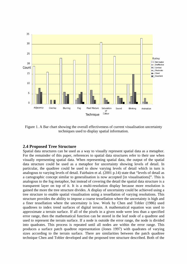
Figure 1. A Bar chart showing the overall effectiveness of current visualisation uncertainty techniques used to display spatial information.

2.4 Proposed Tree Structure Spatial data structures can be used as a way to visually represent spatial data as a metaphor. For the remainder of this paper, references to spatial data structures refer to their use when visually representing spatial data. When representing spatial data, the output of the spatial data structure could be used as a metaphor for uncertainty showing levels of detail. In particular, the quadtree could be used to show varying levels of detail which in turn is analogous to varying levels of detail. Fairbairn et al. (2001 p.14) state that “levels of detail as a cartographic concept similar to generalisation is now accepted [in visualisations]”. This is analogous to the fog metaphor, but instead of covering the detail the spatial data structure is a transparent layer on top of it. It is a multi-resolution display because more resolution is gained the more the tree structure divides. A display of uncertainty could be achieved using a tree structure to enable spatial visualisation using a tessellation of varying resolutions. This structure provides the ability to impose a coarse tessellation where the uncertainty is high and a finer tessellation where the uncertainty is low. Work by Chen and Tobler (1986) used quadtrees to index trend surfaces of digital terrain. A mathematical equation was used to approximate a terrain surface. If all of the pixels in a given node were less than a specified error range, then the mathematical function can be stored in the leaf node of a quadtree and used to represent the terrain surface. If a node is outside the error range, the node is divided into quadrates. This process is repeated until all nodes are within the error range. This produces a surface patch quadtree representation (Jones 1997) with quadrates of varying sizes according to the terrain surface. There are similarities between the patch quadtree technique Chen and Tobler developed and the proposed tree structure described. Both of the

techniques use the quadtree to show a varying resolution based on an uncertainty or error derived from the input data. The rest of this paper is focused on using spatial data structures as a metaphor to show spatial information at its appropriate accuracy level. 2.4.1 Uncertainty in Attributes Using the tree structure to communicate attribute data has a role to play in spatial uncertainty. Two methods were used to achieve an uncertainty value for attributes. This was achieved using values from the 2001 post enumeration survey on the census and then running Monte Carlo simulations. The post survey was employed by Statistics New Zealand to test the quality of the census data, and provide documentation of the census accuracy to users. The survey showed an attribute error for census undercount and geographic location which was stochastically modelled through Monte Carlo, then propagated. The provided geographic attribute uncertainty data was specific to three regions covering New Zealand (South Island, North North Island, South North Island). First a Monte Carlo simulation was run on the undercount information using the sample undercount errors provided. After one hundred simulations, mean and standard deviation layers were created. Next, uncertainty for the census data was obtained using a separate Monte Carlo simulation. The error value used in this simulation varied depending on the geographic location of the current feature in the simulation. There were three possible error values, one for the South Island, northern North Island and southern North Island. The simulation used a normal distribution of random values with a mean of zero and a derived variance for each feature. After performing one hundred iterations for each feature, mean and standard deviation layers were produced. The mean and standard deviation layers from the undercount and census simulations were combined. By dividing the standard deviation layer by the mean layer, a layer of relative error was produced. Monte Carlo simulations were performed for the Dunedin, New Zealand census data using error values associated with the count and undercount values. The simulation also incorporated systematic error that the user of the tool derived. This covered randomness and vagueness uncertainty that could not be accounted for by an error value, as explained in Section 2. The simulation then is able to provide an attribute uncertainty measure for each feature. Using a features attribute uncertainty measure the tree structure can divide appropriately depending on its uncertainty value. 3. Region Quadtree The region quadtree is a hierarchical data structure. It is characterised by the recursive decomposition of space, by subdividing a bounded image array into four equal sized quadrants (Samet 1990). The region quadtree derives from a single root node and is divided into four ordered nodes representing four equal quadrant regions. These nodes can be also divided in turn if the quadrate region is non-homogeneous and continues to be divided until each node has homogeneity. Once each node has homogeneity then that quadrate is stored as a leaf node with its corresponding attributes (Worboys 1995). The region quadtree takes advantage of raster data, homogenous spatial regions and has a variable resolution. 3.1 Using the Region Quadtree to Visualise Uncertainty Samet (1990) exemplifies the region quadtree as decomposing a bounded image array. In the context of this research the region quadtree will be used to decompose census mesh block polygons. The uncertainty of attributes associated with polygons can be conveyed through resolution of data; the less resolution the more uncertain the data is relating to that polygon.

The resolution of the decomposition can be controlled by the uncertainty property of the input data. A demonstration program, The Representation of Uncertainty using Scale-unspecific Tessellations (TRUST) was created to view the uncertainty of spatial information using tree structures. TRUST v1.0 used the region quadtree as the tessellation to represent spatial uncertainty. The programmed steps in TRUST v1.0 to create a region quadtree showing accuracy information are: 1) A Monte Carlo simulation is run to generate uncertainty values for the census data, including the undercount, geographic location and systematic error values for the selected area. 2) The uncertainty data is scaled between 0 – (accurate) and 255 – (uncertain) for easy dissemination of uncertain features; 3) Decomposition takes place using the quadtree structure only if the there is an accurate feature at least 50% inside the quadrate; 4) The accuracy threshold decreases after each division; 5) Recursive division takes place until an accuracy threshold level is met, predetermined by the user. Figure 2 shows a screenshot of TRUST using the region quadtree to visualise attribute uncertainty whilst simultaneously displaying the attribute information. The white figures displayed for theoretical purposes represent the scaled uncertainty, which is proportional to the size of the quadrants. The greater the uncertainty of a feature, the larger the overlaid quadrate becomes.

Figure 2. Using TRUST in the region quadtree tessellation mode to visualise uncertainty information.

3.1.1 Is this a Cartogram of Uncertain Information? Cartograms are defined as value by area maps, and are drawn so that an area’s size is proportional to the value of the attribute it is representing (Dent 1993). The larger the data value the larger the area’s size. Cartograms form an abstraction of geographical reality, losing geographical area, and possibly orientation and contiguity relationships. Also there is no need to categorise data as a choropleth does; the quantitative information is visually displayed. These properties are similar to the method described in Section 3.1 where the region quadtree is used to visualise uncertainty information. Instead of an area of a vector

polygon representing attribute magnitude, this paper uses square quadtree elements to do the same. The square was chosen to create the abstraction of uncertainty information, in effect losing geographical area and orientation. The region quadtree maintains each quadrate’s size proportional to the amount of uncertainty and the tessellations are adjacent the same as contiguous cartograms. The representations do differ; the example in Figure 2 demonstrates that there is a one-to-one, a one-to-many or a many-to-many relationship between an area and the amount of squares, but a cartogram maintains one shape per area relationship. Also the attribute data is preserved and undistorted (i.e. the relationship of uncertainty to area is scaled so as to minimize displacement of adjacent areas) allowing for the uncertainty information to be simultaneously displayed over it. In other words, the pseudo-spatial extents of the attribute data and related uncertainty data remain approximately the same. 4. Other Possible Data Structures to Visualise Uncertainty Information This paper discusses two other possible data structures that could be used to visualise spatial uncertainty, the hexagonal heptree and the HoR quadtree. For geovisualisation, Carr et al. (1992) states that hexagons have two advantages over squares, visual appeal and representational accuracy. Also, the horizontal and vertical visual lines created by square tessellations can have a strong effect on humans due to our internal sense of gravitational balance. Therefore the horizontal and vertical lines generated by square tessellations in standard orientation are irritating to view and are less preferred. Instead, the hexagonal heptree or the HoR quadtree could be a possible tree structure to use for geovisualisation. 4.1 The Hexagonal Heptree Bell et al. (1983) discuss a number of different tilings that can occur over a surface. One such tiling is the hexagonal heptree commonly called the 7-shape. It is a regular tiling or a regular polygon where all sides are of equal length as are the interior angles (Samet 1990). The hexagonal heptree is also a limited tiling, the tiling hierarchy becomes dissimilar; a partition cannot be infinitely decomposable into smaller patterns. To exemplify, seven hexagons can be arranged in a “rosette” (Laurini and Thompson 1992) which only approximates to the unit hexagon shape (Figure 3). In turn, seven of these rosettes can be arranged to create recursively larger hexagon approximations. It is possible to have combinations of limited and unlimited, and regular and irregular tilings. Bell et al. (1983) state that there are only 4 unlimited tilings that are infinitely decomposable into smaller patterns, being the quadtree and any square tessellation, equilateral triangles, isosceles triangles, and the 30-60 right triangle. The quadtree and equilateral triangles are regular whilst the other two respectively are not.

Figure 3. Hexagonal heptree using a 7-rosette shape. (Boots 1999).

4.2 The HoR Quadtree The hexagonal heptree has limitations. It is not an unlimited tiling, the pattern changes at the lowest level of the tree. Also when the conventional hexagonal heptree is divided, each recursive child is rotated by an unjustified angle in relation to its parent (Bell et al. 1987; Samet 1990; Holroyd and Bell 1992). This can produce visual confusion with too many angles making the tessellation harder to create and index. The HoR structure (Figure 4) was designed by Bell et al. (1987) to remove the dividing limitation of a standard hexagon. Also the HoR quadtree does not have any rotational differences between child and parent shapes. After amalgamating the centroids of 4 hexagons or 4 rhombi, the HoR quadtree forms an identical pattern. The rhombi pattern is unlimited, and is infinitely decomposable, but the hexagonal pattern is limited when at the lowest level, as shown in Figure 4a. Also, Boots (1999) states that the HoR addressing system has advantages over the hexagonal heptree system.

a. b.

Figure 4. The Hexagonal or Rhombi (HoR) quadtree tessellation. (a) Shows the hexagonal tessellation at the atomic level, and combined hexagonal rhombi at higher levels. (b) Shows

the rhombus tessellation. Modified from Bell et al. (1987).

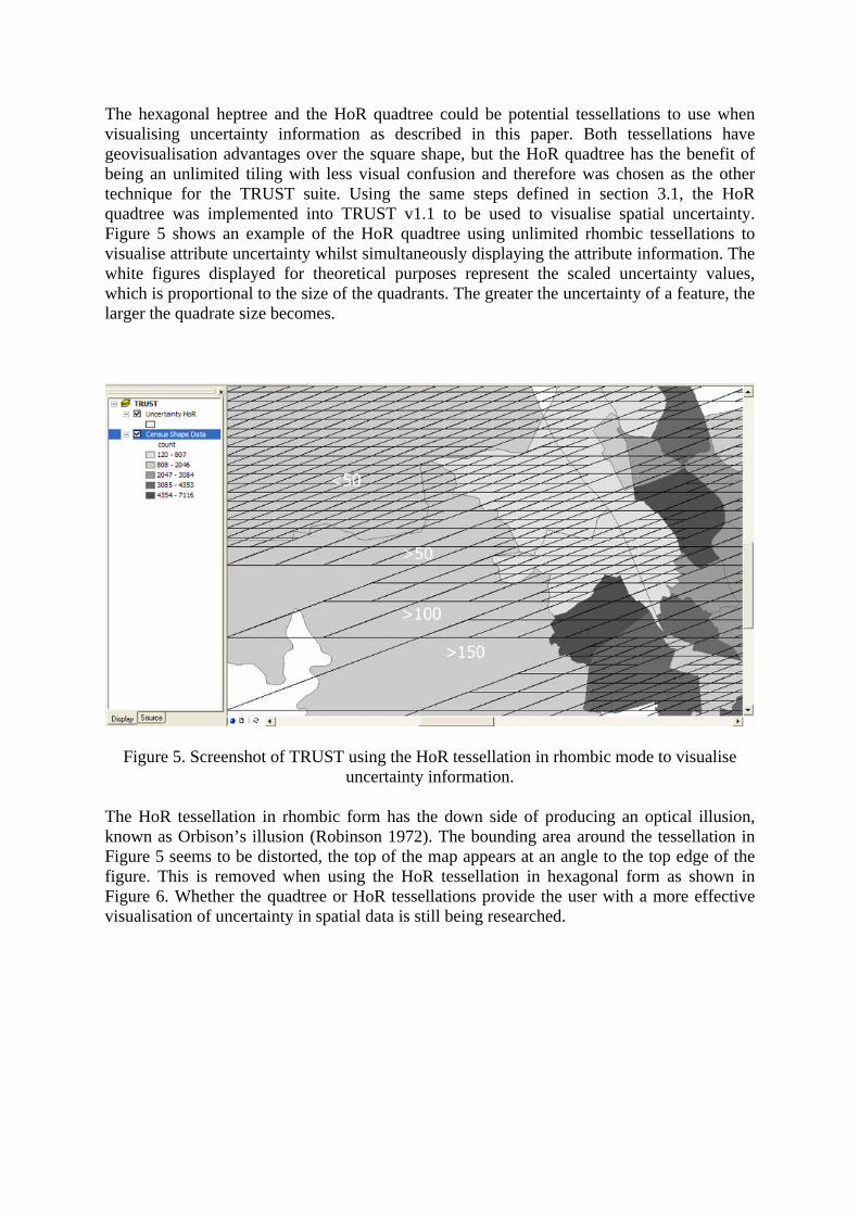
The hexagonal heptree and the HoR quadtree could be potential tessellations to use when visualising uncertainty information as described in this paper. Both tessellations have geovisualisation advantages over the square shape, but the HoR quadtree has the benefit of being an unlimited tiling with less visual confusion and therefore was chosen as the other technique for the TRUST suite. Using the same steps defined in section 3.1, the HoR quadtree was implemented into TRUST v1.1 to be used to visualise spatial uncertainty. Figure 5 shows an example of the HoR quadtree using unlimited rhombic tessellations to visualise attribute uncertainty whilst simultaneously displaying the attribute information. The white figures displayed for theoretical purposes represent the scaled uncertainty values, which is proportional to the size of the quadrants. The greater the uncertainty of a feature, the larger the quadrate size becomes.

Figure 5. Screenshot of TRUST using the HoR tessellation in rhombic mode to visualise uncertainty information.

The HoR tessellation in rhombic form has the down side of producing an optical illusion, known as Orbison’s illusion (Robinson 1972). The bounding area around the tessellation in Figure 5 seems to be distorted, the top of the map appears at an angle to the top edge of the figure. This is removed when using the HoR tessellation in hexagonal form as shown in Figure 6. Whether the quadtree or HoR tessellations provide the user with a more effective visualisation of uncertainty in spatial data is still being researched.

Figure 6. Screenshot of TRUST using the HoR tessellation in hexagonal mode to visualise uncertainty information.

5. Summary Current literature in geovisualisation (Fairbairn et al. 2001; MacEachren and Kraak 2001; Zhang and Goodchild 2002), has expressed the need to visualise uncertainty, whether it be a supplement to existing data or a visualisation in its own right. A propagated uncertainty measure of census data has been derived using the Monte Carlo simulation statistical method. This can provide a good overall approach to analysing error in census data because of its straight statistical methodology. Also the use of a Gaussian distribution is ideal when dealing with a large number of random factors contributing to error, something census data can have. The focus of this research has been to use hierarchical spatial data structures such as quadtrees and the HoR to visualise attribute uncertainty in spatial data. Quadtrees can have a multi-resolution display, and this has been used as a metaphor of detail for visualising attribute uncertainty. The more accurate an area, the more the data structure will divide, and therefore the smaller the resolution. In the converse case it could be argued that the tessellations could be made sufficiently dense so as to hide the attribute data, working in a similar way to the fog metaphor – this scenario will be explored. The region quadtree was discussed as a potential way to visualise uncertainty using an uncertainty measure derived from a Monte Carlo simulation. Other potential tessellation shapes are the hexagonal heptree and HoR quadtree to visualise uncertainty information. These have geovisualisation advantages over the conventional region quadtree. User testing on all these hierarchical data structure uncertainty representations (using much the same data collection format as described in section 2.2.1) will be an important task in the near future. Even the finest resolution cell in the uncertainty quadtree looks coarse when compared with the relatively precise choropleth boundaries that it overlays. These crisp-looking boundaries are misleading, as they imply that there is a stepwise progression of attribute value across the boundary line, when a smoother function is normally the case. Therefore, the coarse boundaries implicit in the quadtree, which divide neighbouring polygon uncertainties, are entirely appropriate.

Fairbairn et al (2001) has also included multi-scale visualisation on the geovisualisation research agenda. With this in mind, there is an irony in using a multi-resolution structure such as a quadtree for something other than spatial location, effectively suppressing the multi-scale modelling capacity of the quadtree. Using a quadtree cell, not as a representation of geographical area, but as being proportional to uncertainty, is essentially the definition of a cartogram. 6. Acknowledgements This work would not be possible without funding from the School of Business at the University of Otago. 7. References BELL, S. B. M., B. M. DIAZ and F. C. HOLROYD (1987). The HoR quadtree: An optimal

structure based on a non-square 4-shape. Mathematics in Remote Sensing. S. R. Brooks. Chelmsford, Clarendon Press, Oxford.

BELL, S. B. M., B. M. DIAZ, F. C. HOLROYD and M. JACKSON (1983). “Spatially referenced methods of processing raster and vector data.” Image and Vision Computing 1(4): pp. 211-220.

BOOTS, B. (1999). Spatial Tessellations. Geographic information systems and science. P. Longley, M. F. Goodchild, D. J. Maguire and D. W. Rhind. Chichester ; New York, Wiley: xviii, 454.

BURROUGH, P. A. and R. MCDONNELL (1998). Principles of geographical information systems. Oxford ; New York, Oxford University Press.

CARR, D. B., A. R. OLSEN and D. WHITE (1992). “Hexagon Mosaic Maps for Display of Univariate and Bivariate Geographical Data.” Cartography and Geographic Information Systems 19(4): pp. 228-236.

CHEN, Z.-T. and W. R. TOBLER (1986). Quadtree Representation of Digital Terrain. Auto-Carto 6 Proceedings:, London.

DE GRUIJTER, J. J., D. J. J. WALVOORT and P. F. M. VAN GAANS (1997). “Continuous soil maps -- a fuzzy set approach to bridge the gap between aggregation levels of process and distribution models.” Geoderma 77(2-4): 169-195.

DENT, B. D. (1993). Cartography : thematic map design. Dubuque, Iowa, Wm. C. Brown Publishers.

EHLSCHLAEGER, C. R. (2002). Can we construct error buttons for every application? Proceedings : International Symposium on Spatial Accuracy in Natural Resources and Environmental Science10-12 July 2002, Melbourne, Australia, University of Melbourne and RMIT University.

EHLSCHLAEGER, C. R., A.M. SHORTRIDGE and M. F. GOODCHILD (1997). “Visualizing spatial data uncertainty using animation.” Computers and Geosciences 23(4): 387-395.

EVANS, B. J. (1997). “Dynamic display of spatial data reliability: does it benefit the Map user?” Computers and Geosciences 23(4): p. 409-422.

FAIRBAIRN, D., G. ANDRIENKO, N. ANDRIENKO, G. BUZIEK and J. DYKES (2001). “Representation and its Relationship with Cartographic Visualization.” Cartography and Geographic Information Science 28(1): pp. 13-28.

FISHER, P. (1993). “Visualizing uncertainty in soil maps by animation.” Cartographica 30(2-3): p. 20-27.

FISHER, P. (1994). “Hearing the Reliability in Classified Remotely Sensed Images.” Cartography and Geographical Information Systems 21(1): pp. 31-36.

FISHER, P. and K. C. MCGWIRE (2001). Spatially Variable Thematic Accuracy: Beyond the Confusion Matrix. Spatial uncertainty in ecology : implications for remote sensing and GIS applications. C. T. Hunsaker. New York, N.Y., Springer: xiii, 402.

GOODCHILD, M. F. (1994). GIS error models and visualization techniques for spatial variability in soils. Proceedings 15th International Congress of Soil Science, Acapulco, July 10-16, 1994.

HENGL, T., D. J. J. WALVOORT and A. BROWN (2002). Pixel and Colour Mixture: GIS techniques for visualisation of fuzzyness and uncertainty of natural resource inventories. Proceedings : International Symposium on Spatial Accuracy in Natural Resources and Environmental Science10-12 July 2002, Melbourne, Australia, University of Melbourne and RMIT University.

HOLROYD, F. C. and S. B. M. BELL (1992). “Raster GIS: Models of Raster Encoding.” Computers and Geosciences 1(4): pp. 419-426.

JONES, C. B. (1997). Geographical information systems and computer cartography. Harlow, Longman.

KRYGIER, J. B. (1994). Sound and Geographic Visualization. Visualization in the Modern Cartography. A. MacEachren and D. R. F. Taylor. New York, Pergamon: pp. 149-166.

LAURINI, R. and D. THOMPSON (1992). Fundamentals of spatial information systems. London ; New York, Academic Press.

LONGLEY, P., M. F. GOODCHILD, D. J. MAGUIRE and D. W. RHIND (2001). Geographic information systems and science. Chichester ; New York, Wiley.

MACEACHREN, A., C. A. BREWER and L. W. PICKLE (1998). “Visualizing georeferenced data: representing reliability of health statistics.” Environment and Planning A 30: p1547-1561.

MACEACHREN, A. and M.-J. KRAAK (2001). “Research Challenges in Geovisualisation.” Cartography and Geographic Information Science 28(1): pp. 3-12.

MACEACHREN, A. M. (1992). “Visualizing Uncertain Information.” Cartographic Perspective 13(Fall): pp. 10-19.

MONMONIER, M. and M. GLUCK (1994). “Focus groups for design improvement in dynamic cartography.” Cartography and Geographical Information Systems 21(1): p. 37-47.

PEUQUET, D. J. (2002). Representations of space and time. New York, Guilford Press. ROBINSON, J. (1972). The psychology of visual illusion. London,, Hutchinson. ROSENFELD, A. and H. SAMET (1985). Tree Structures for Region Representation. Auto-

Carto 7 : proceedings : digital representations of spatial knowledge : Washington, D.C., March 11-14, 1985, Falls Church, Va., American Society of Photogrammetry ; American Congress on Surveying and Mapping.

SAMET, H. (1990). The design and analysis of spatial data structures. Reading, Mass., Addison-Wesley.

STATISTICS NEW ZEALAND. (2002). A Report on the Post Enumeration Survey 2001. Wellington, Statistics New Zealand: 41.

WORBOYS, M. (1995). GIS : a computing perspective. London ; Bristol, Pa., Taylor & Francis.

ZHANG, J. and M. F. GOODCHILD (2002). Uncertainty in geographical information. London ; New York, Taylor & Francis.