Visual Terrain Classi cation For Legged Robotskatiebyl/papers/Filitchkin_MSThesis.pdfterrain images...

UNIVERSITY OF CALIFORNIASanta Barbara

Visual Terrain Classification For Legged Robots

A Thesis submitted in partial satisfactionof the requirements for the degree of

Master of Science

in

Electrical and Computer Engineering

by

Paul Filitchkin

Committee in Charge:

Professor Katie Byl, Chair

Professor Joao Hespanha

Professor B.S. Manjunath

December 2011

The Thesis ofPaul Filitchkin is approved:

Professor Joao Hespanha

Professor B.S. Manjunath

Professor Katie Byl, Committee Chairperson

September 2011


Copyright c© 2011

by

Paul Filitchkin

iii

Abstract


Paul Filitchkin

Recent work in terrain classification has relied largely on 3D sensing meth-

ods and color based classification. We present an approach that works with a

single, compact camera and maintains high classification rates that are robust

to changes in illumination. Terrain is classified using a bag of visual words

(BOVW) created from speeded up robust features (SURF) with a support vec-

tor machine (SVM) classifier. We present several novel techniques to augment

this approach. A gradient descent inspired algorithm is used to adjust the SURF

Hessian threshold to reach a nominal feature density. A sliding window tech-

nique is also used to classify mixed terrain images with high resolution. We

demonstrate that our approach is suitable for small legged robots by perform-

ing real-time terrain classification on LittleDog. The classifier is used to select

between predetermined gaits for traversing terrain of varying difficulty. Results

indicate that real-time classification in the loop is faster than using a single

all-terrain gait.

iv

Contents

Abstract iv

List of Figures vii

List of Tables viii

1 Terrain Classification 11.1 Introduction . . . . . . . . . . . . . . . . . . . . . . . . . . . . . 1

1.1.1 Executive Summary . . . . . . . . . . . . . . . . . . . . 21.2 Terminology . . . . . . . . . . . . . . . . . . . . . . . . . . . . . 41.3 Algorithms . . . . . . . . . . . . . . . . . . . . . . . . . . . . . . 7

1.3.1 Feature Extraction . . . . . . . . . . . . . . . . . . . . . 71.3.2 Generating a Vocabulary . . . . . . . . . . . . . . . . . . 91.3.3 Homogeneous Classification . . . . . . . . . . . . . . . . 101.3.4 Heterogeneous Classification . . . . . . . . . . . . . . . . 11

1.4 Software Architecture . . . . . . . . . . . . . . . . . . . . . . . . 131.4.1 Structural Organization . . . . . . . . . . . . . . . . . . 141.4.2 Database Initialization . . . . . . . . . . . . . . . . . . . 151.4.3 Populating Features . . . . . . . . . . . . . . . . . . . . 171.4.4 Populating Vocabulary . . . . . . . . . . . . . . . . . . . 19

1.5 Offline Experiments . . . . . . . . . . . . . . . . . . . . . . . . . 201.5.1 Datasets . . . . . . . . . . . . . . . . . . . . . . . . . . . 201.5.2 Methodology . . . . . . . . . . . . . . . . . . . . . . . . 231.5.3 Results . . . . . . . . . . . . . . . . . . . . . . . . . . . . 24

2 Applications 302.1 System Overview . . . . . . . . . . . . . . . . . . . . . . . . . . 31

2.1.1 High-level planning . . . . . . . . . . . . . . . . . . . . . 31

v

2.1.2 Terrain Classification . . . . . . . . . . . . . . . . . . . . 332.1.3 Gait Generation . . . . . . . . . . . . . . . . . . . . . . . 35

2.2 Real-Time Experiments . . . . . . . . . . . . . . . . . . . . . . 362.2.1 Procedures . . . . . . . . . . . . . . . . . . . . . . . . . . 362.2.2 Results . . . . . . . . . . . . . . . . . . . . . . . . . . . . 39

2.3 Conclusion . . . . . . . . . . . . . . . . . . . . . . . . . . . . . . 422.4 Future Work . . . . . . . . . . . . . . . . . . . . . . . . . . . . . 43

Bibliography 45

vi

List of Figures

1.1 Executive Summary of Results . . . . . . . . . . . . . . . . . . . 31.2 High Feature Count Variance Using a Constant Hessian Threshold 71.3 Data Oraganization . . . . . . . . . . . . . . . . . . . . . . . . . 141.4 Database Initialization Flowchart . . . . . . . . . . . . . . . . . 161.5 Populate Features Flowchart . . . . . . . . . . . . . . . . . . . . 171.6 Extract Features Flowchart . . . . . . . . . . . . . . . . . . . . 181.7 Populate Vocabulary Flowchart . . . . . . . . . . . . . . . . . . 191.8 Terrain Classes . . . . . . . . . . . . . . . . . . . . . . . . . . . 201.9 Dataset Image Dimensions . . . . . . . . . . . . . . . . . . . . . 211.10 Example of SURF key points and color histograms . . . . . . . 221.11 Word experiment verification results . . . . . . . . . . . . . . . 251.12 K-means (a) and feature experiment (b) results . . . . . . . . . 261.13 Size experiment verification and time performance . . . . . . . . 271.14 Heterogeneous Classification Results . . . . . . . . . . . . . . . 29

2.1 Boston Dynamics LittleDog Robot . . . . . . . . . . . . . . . . 302.2 Matlab Process . . . . . . . . . . . . . . . . . . . . . . . . . . . 322.3 Real-time Execution Cycle . . . . . . . . . . . . . . . . . . . . . 332.4 Terrain Classification Process . . . . . . . . . . . . . . . . . . . 342.5 Gait Generation Process . . . . . . . . . . . . . . . . . . . . . . 352.6 LittleDog Gaits . . . . . . . . . . . . . . . . . . . . . . . . . . . 362.7 LittleDog Experiment Terrain . . . . . . . . . . . . . . . . . . . 372.8 LittleDog Traversing the Large Rocks Terrain Class . . . . . . . 392.9 Terrain Traversal Performance . . . . . . . . . . . . . . . . . . . 402.10 Real Time Classification Results . . . . . . . . . . . . . . . . . . 41

vii

List of Tables

1.1 Heterogeneous Classification Definitions . . . . . . . . . . . . . . 121.2 List of Parameter Tuning Experiments . . . . . . . . . . . . . . 231.3 Feature Extraction Performance . . . . . . . . . . . . . . . . . . 28

viii

Chapter 1

Terrain Classification

1.1 Introduction

Terrain classification is a vital component of autonomous outdoor naviga-

tion, and serves as the test bed for state-of-the-art computer vision and machine

learning algorithms. This area of research has gained much popularity from the

DARPA Grand Challenge [23] as well as the Mars Exploration Rovers [6].

Recent terrain classification and navigation research has focused on using a

combination of 3D sensors and visual data [23] as well as stereo cameras [7] [16].

The work in [5] uses vibration data from onboard sensors for classifying terrain.

Most of this work has been applied to wheeled robots, and other test platforms

have included a tracked vehicle [15] and a hexapod robot [7]. On the computer

vision spectrum of research, interest in terrain classification has been around

as early as 1976 [24] for categorizing satellite imagery. More recent work has

1

Chapter 1. Terrain Classification

focused on the generalized problem of recognizing texture. Terrain and texture

classification falls into the following categories: spectral-based [13] [22] [21] [1],

color-based [23] [8], and feature-based [2].

Over the last decade, a large volume of work has been published on scale

invariant feature recognition and classification. Scale invariant features have

proven to be very repeatable in images of objects with varying lighting, viewing

angle, and size. They are robust to noise and provide very distinctive descriptors

for identification. They are suitable for both specific object recognition [18] [11]

[19] as well as broad categorization [9] [10].

1.1.1 Executive Summary

In this work we use the SURF algorithm to extract features from terrain, a

bag of visual words to describe the features, and a support vector machine to

classify the visual words. Using this approach we were able to identify, with up

to 95% verification accuracy, 6 different terrain types as shown in Figure 1.1(a).

Our method was also able to maintain high verification accuracy with changes

in illumination whereas color-based classification performed much worse. We

also tested a novel approach for regionally classifying heterogeneous (mixed)

terrain images. A support vector machine classifier trained on homogeneous

2


terrain images was used to classify regions on the images. A voting procedure

was then used to determine the class of each pixel.

Real-time classification of homogeneous terrain was performed using the

LittleDog quadruped robot. Terrain classification was used to select one of

three predetermined gaits for traversing 5 different types of terrain. We were

able to show that classification in-the-loop with dynamic gait selection allowed

the robot to traverse terrain faster than using an all-purpose gait (Gait C)

1.1(b). Traversing the most difficult terrain actually required the all-purpose

gait so in that particular case the classification slowed the robot.

192 256 320 384 448 512 57655

60

65

70

75

80

85

90

95

100

Verification Accuracy Versus Image Dimension

Ver

ifica

tion

Acc

urac

y (P

erce

nt)

Square Image Side Dimension (pixels)

BOVWColorBOVW (underexposed)Color (underexposed)

Small Rocks Chips/Big Rocks Grass Rubber Tile0

5

10

15

20

25

30

35

40

45

50

Gait C vs. Classification in the Loop Traversal Times

Tim

e (s

econ

ds)

All−Purpose Classification

Figure 1.1: Executive Summary of Results

3


1.2 Terminology

This work uses terminology from machine learning and computer vision

along with a few non-standard terms that have been adapted for this applica-

tion. This section includes an overview of key terms and their meanings. Many

image classification techniques were historically adapted from natural language

processing and text categorization. For the interested reader, Chapter 16 in [17]

provides an introduction to this field.

A supervised learning framework is applied in this paper where a set of

labeled data is used to train a classifier in an offline environment. Verification

is then performed on the classifier by using a different set of labeled test data.

Image classification is accomplished by first preprocessing an image, I ∈ Rm×n,

to generate a vector x ∈ RM which compactly describes the image. The vector

becomes the input to the classifier f(·) which outputs a label ì ∈ L, in the

form f(x) = ì. Where L ⊂ Z and ì is mapped to some description of the class

where i is the index of the class. The most basic example of this approach is to

compute the color histogram of an image and use a naıve Bayesian network to

determine the class.

In this text, we focus on using features to describe an image. A feature is a

unique point of interest on an image with an accompanying set of information.

4


For the purpose of this work, it is implied that each feature consists of a key

point and a descriptor. The key point includes information such as the pixel

coordinate, scale, and orientation. The descriptor (also referred to as a feature

vector), d ∈ RN , contains real values that uniquely describe a neighborhood lo-

cal to a key point. Two popular methods for generating features include scale

invariant feature transform (SIFT) [14] and speed up robust features

(SURF) [4]. Each algorithm maintains some degree of invariance to scale, in-

plane rotation, noise, and illumination. Both algorithms were used in initial

testing for this work, and the SURF algorithm was found to have better speed

and slightly better verification accuracy. This is a well established result that

was initially reported by Bay et. al. in [4]. Throughout the remainder of this

work we will focus primarily on SURF, and unless specified otherwise, the term

feature will be used to imply a key point and 64-element descriptor pair gener-

ated by the SURF algorithm. The process of feature extraction is broken up

into two steps: feature detection and feature computation. Feature detection

consists of finding stable key points in the image and feature computation is

the process of creating descriptors for each key point.

In this context a visual word is a descriptor, v ∈ RM from a finite set V ,

that can be used to approximate an image descriptor, x ∈ RM . Each image

descriptor can be mapped to the ith visual word vi such that vi ←→ x. The

5


set V is called the vocabulary (or visual vocabulary). In this work we use the

bag of visual words (BOVW) data structure to describe each image (also

commonly referred to as a bag of features or a bag of key points). This data

structure discards ordering and spatial information and as a result no geometric

correspondence between key points and descriptors is preserved. We represent

the BOVW by a histogram that tallies the number of times a word appears in

a particular image.

In this work the classification problem is separated into two categories: clas-

sifying homogeneous and heterogeneous images. A homogeneous image is one

that contains a single type of terrain and is assigned one class label whereas in

a heterogeneous context the image contains different patches of terrain that

each have a corresponding label. The term populate takes on a non-standard

definition throughout this work and is used to mean the process of generating or

loading data. In particular, the term is used to describe the process of loading

cached data from disk if it exists or otherwise computing it from scratch.

6


1.3 Algorithms

1.3.1 Feature Extraction

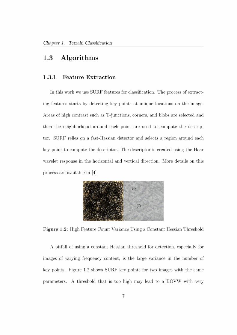
In this work we use SURF features for classification. The process of extract-

ing features starts by detecting key points at unique locations on the image.

Areas of high contrast such as T-junctions, corners, and blobs are selected and

then the neighborhood around each point are used to compute the descrip-

tor. SURF relies on a fast-Hessian detector and selects a region around each

key point to compute the descriptor. The descriptor is created using the Haar

wavelet response in the horizontal and vertical direction. More details on this

process are available in [4].

Figure 1.2: High Feature Count Variance Using a Constant Hessian Threshold

A pitfall of using a constant Hessian threshold for detection, especially for

images of varying frequency content, is the large variance in the number of

key points. Figure 1.2 shows SURF key points for two images with the same

parameters. A threshold that is too high may lead to a BOVW with very

7


little data and threshold that is too low will flood the classifier with redundant

information and noise. In order to combat this problem we propose a gradient

descent inspired threshold adjuster. Let n = d(h) where d(·) is an unknown

function that returns the number of key points, n, for a given Hessian threshold

h. While the rate of change is not known, d(·) is a monotonically decreasing

function. To find the threshold that produces a desired key point count, h′, an

iterative convex optimization is performed. For a given step i the error can be

written as e(i) = d(hi) − d(h′) and our goal is to minimize this quantity. We

use an update method similar to gradient descent, but instead of computing the

function’s gradient we use the error value divided by the local rate of changes,

e(i)|hi−hi−1| . Equation 1.1 is the threshold update step where α is a user set value

that determines the update rate.

hi+1 = hi + αd(hi)− d(h′)

|hi − hi−1|(1.1)

In practice this approach has the potential to overshoot the target key point

count, d(h′), by changing the threshold too rapidly. When an overshoot con-

dition is detected, the new threshold becomes the average of the previous two

and the update rate is halved.

8


1.3.2 Generating a Vocabulary

To generate a vocabulary, we use the k-means clustering algorithm with the

initialization procedure outlined in [3]. In the context of this work, the k-means

problem is to find an integer number of centers that best describe groupings of

descriptor data. More formally: let k ∈ Z be the desired number of clusters and

let X ⊂ RM be the set of descriptors. The goal is to find k centers (descriptors)

in C ⊂ RM that minimize φ (Equation 1.2).

φ =∑x∈X

minc∈C||x− c||2 (1.2)

The iterative k-means algorithm (Lloyd’s algorithm) for achieving this operates

as follows: given centers C assign each descriptor x ∈ X to the c ∈ C that has

the smallest Euclidean distance. Then each center is repeatedly recomputed

until the centers stop shifting. This procedure will always terminate, but in

practice it is common to set a maximum allowable number of iterations. The

work in [3] provides an effective initialization procedure that decreases computa-

tion time. The authors call this algorithm k-means++ which uses a probabilistic

initialization procedure followed by Lloyd’s algorithm. In k-means++ the initial

center c1 ∈ C is chosen uniformly at random from X and subsequent points ci

are chosen with the probability in Equation 1.3. Where D(x) is the distance

9


between x and the nearest center cj that has already been chosen (0 < j < i).

P (ci = x′ ∈ X) =D(x′)2∑x∈X D(x)2

(1.3)

This approach tends to select centers that are further away from the ones that

have already been chosen. The idea is to keep a high variance within the centers,

but maintain some probability of not always choosing the furthest point.

1.3.3 Homogeneous Classification

Once a visual vocabulary has been created each image can be described by a

word frequency vector. First, a vocabulary word vi is assigned to each descriptor

dj in the image by choosing the i that minimizes ||vi − dj||. This process

essentially approximates each descriptor with the vocabulary word that has the

nearest Euclidean distance. Each word is then counted and the frequency of

each word is stored in a vector q ∈ Zn where n is the number of visual words.

Images in the training set each have a corresponding frequency vector and are

used to train the linear SVM classifier.

The training goal of a linear SVM is to find a hyperplane that provides the

maximum margin of separation between classes. Let the training set consist of

k points (qi, yi) indexed by i where yi determines if the word frequency vector

10


belongs to the given class. If it belongs to the class then yi = 1 otherwise

yi = −1. Any hyperplane that separates the data can be described by all

vectors, h, that satisfy w · h − b = 0 where w is the vector normal to the

hyperplane and b is a scalar bias. The solution for the optimal hyperplane is

achieved through quadratic programming using the constraints in Equation 1.4.

minw,b,ξ

{1

2||w||2 − p

k∑i=1

ξi

}

subject to yi(wTqi + b) ≥ 1− ξi

ξi ≥ 0

(1.4)

Where p > 0 is the penalty parameter of the error term. A more complete

and generalized introduction to SVMs is provided in [12]. Once a hyperplane

is computed for each class, the intersections are used to describe the decision

boundaries for the classifier.

1.3.4 Heterogeneous Classification

In order to classify a heterogeneous terrain image, it is necessary to gener-

ate features with an approximately constant density across all pixels. This is

achieved by dividing the image into squares and applying feature extraction on

each square independently. The feature sets for each square are then combined

11


Table 1.1: Heterogeneous Classification Definitions

Symbol Description

I Input image, I ∈ Rm×n

C Set of classification centers (pixels) where C ⊂ R2

r, ro Radius in (fractional) pixels, r, ro ∈ RF The set of all features for an image I

Fc,r All features around c ∈ C with radius ||c|| < r

L The set of all class labels in the dataset

V` Matrix of votes for label ` ∈ L, V` ∈ Zm×n

R Matrix with classification results, R ∈ Zm×n

sa Grid spacing for feature extraction in pixels

sb Grid spacing for classification points in pixels

n Desired range (min/max) of features within radius, n ∈ Z2

to form a single feature set. Afterwards, points on the image are selected on

a constant grid and classification is performed in each neighboring region. At

each point we iteratively resize a ball so that it encompasses the target number

of features (within some tolerance). This procedure is very similar to the gra-

dient descent inspired algorithm mentioned in Section 1.3.1. Let ri represent

the radius of the ball at the ith iteration and let D(ri) represent the number

of features exclusively inside the ball. The term D(r′) is the desired number of

features where r′ is the unknown radius of interest. To find r′ we use Equation

1.5 which includes a user selectable update rate, α.

ri+1 = ri + αD(ri)−D(r′)

|ri − ri−1|(1.5)

12


Once a suitable number of features is encircled, a word histogram vector is gen-

erated, and classification is performed using the linear SVM classifier trained on

homogeneous terrain images. All pixels exclusively in the circle are labeled with

the classification result and this step is repeated about each point. Afterwards

a voting procedure is applied to each pixel by tallying the number of votes for

each class. This procedure is outlined in pseudo code in Algorithm 1.

Algorithm 1 Heterogeneous Terrain Classification1 r ← ro2 F ← ExtractGridFeatures(I, sa)3 C ← GenerateClassificationPoints(I, sb)4 for all c ∈ C do5 (Fc,r, r)← FindRegionalFeatures(C,F,n, r)6 `← Classify(Fcr)7 V` ← Vote(V`, c, r)8 end for9 for all ` ∈ L do10 R← CountVotes(V`, R)11 end for

1.4 Software Architecture

The following section describes the high-level software architecture used in

this work. The reader who is more interested in the experiments and results

can skip to Section 1.5.

13


Vocabulary

Label ID to

Name Map

Database

Setup Variables• Vocabulary options

• Feature detector/extractor options

• Color classifier options

• Visual word classifier options

• Caching enabled

• Logging enabledColor

Classifier

Visual Word

Classifier

Array of Entries (one entry per image)

...

Entry

Unique NameImage

FilenamesLabel ID

Comment

(optional)

Image

Dimensions

Keypoints

Descriptors

FeaturesBag of visual

words

Histogram

Color

Histogram

Feature

detector

Feature

extractor

Database

Paths

Figure 1.3: Data Oraganization

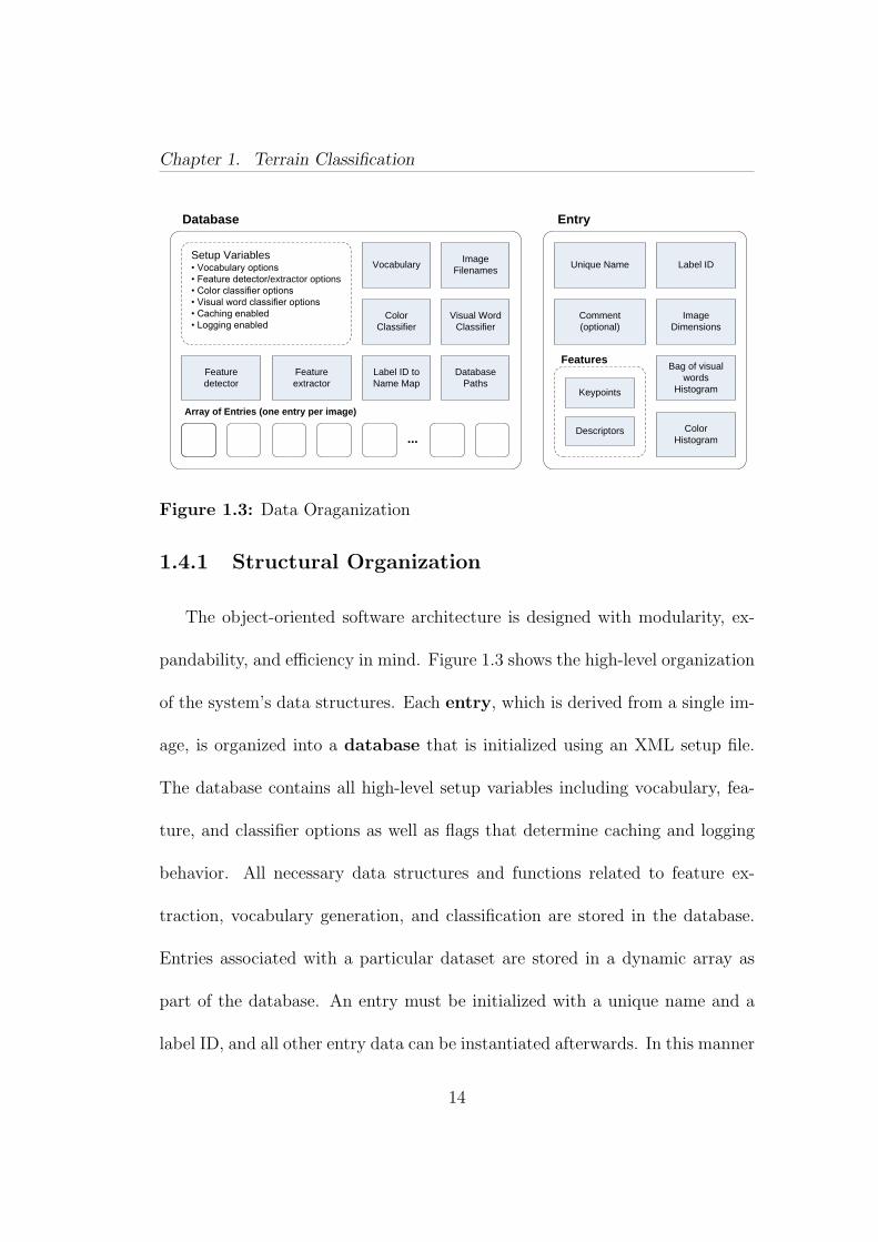
1.4.1 Structural Organization

The object-oriented software architecture is designed with modularity, ex-

pandability, and efficiency in mind. Figure 1.3 shows the high-level organization

of the system’s data structures. Each entry, which is derived from a single im-

age, is organized into a database that is initialized using an XML setup file.

The database contains all high-level setup variables including vocabulary, fea-

ture, and classifier options as well as flags that determine caching and logging

behavior. All necessary data structures and functions related to feature ex-

traction, vocabulary generation, and classification are stored in the database.

Entries associated with a particular dataset are stored in a dynamic array as

part of the database. An entry must be initialized with a unique name and a

label ID, and all other entry data can be instantiated afterwards. In this manner

14


only the necessary task-specific data is stored. Consequently, a database that

only needs to classify terrain based on color does not need to store feature data

in each entry. For space and time efficiency only the identification number cor-

responding to a verbal label is stored in an entry. The name is translated via an

ID to name map in the database. This organization structure is convenient for

our supervised learning approach in that a one labeled database can be created

as a training set and the other can be created as a test set. The test set can

then be easily verified against the training set and verification statistics can be

readily computed. In the case where an unlabeled image needs to be classified

an independent entry with a null label ID can be classified against a database.

If a vocabulary is available then only the visual word histogram needs to be

stored in an entry. This makes transmitting and storing entries very memory

efficient since the raw descriptors do not need be kept in memory.

1.4.2 Database Initialization

Figure 1.4 represents the initialization procedure for a database which re-

quires the aforementioned XML setup file and database paths. The database

paths provide a very convenient way of organizing database images, log out-

put directories, caching directories, and setup files. For example, by changing

the caching directory all previous cached data can be preserved while different

15


Parse setup

file

Create

Database

Database Paths

(setup, image, logs,

cache directories)

Generate

setup

summary log

XML setup file

Setup parameters

valid?

Populate

Features

Populate

Vocabulary

Train Visual

Word

Classifier

Populate

Color

Histograms

Train Color

Classifier

Display

Error

Cached Features

Cached Vocabulary

Cached Histograms

YesNo

Figure 1.4: Database Initialization Flowchart

settings are used to generate a new database. Most system-level settings can

be easily changed in the XML file without having to recompile the software.

This provides a very convenient way of running experiments and documenting

trials. Once setup parameters have been parsed a time-stamped setup summary

is saved to disk containing a list of all parameters used. Afterwards, the color

and visual word classifiers are initialized. Setup for the visual word classifier is

characterized by three steps: extracting the features, creating a vocabulary, and

training the classifier. Preparations for the color classifier consist of populating

color histograms and training the classifier. The following sections provide a

more detailed explanation of several database initialization tasks.

16


Load image

Cached feature

exists?

Cached feature up to

date?

Load cached

feature

Perform contrast

stretching?

Extract SIFT

Features

Adjuster

enabled?

Compute features on

a grid?

Split into

sub-images

For each sub-image

Feature type

SIFT

SURF

Perform

contrast

stretching

Extract SURF

features with

adjuster

Cache

Features?

Write

features to

disk

For each

filename

Extract SURF

features

Yes

Yes

Yes

YesNo

No Yes

No No

No

Create Log?Write log to

disk

No

Yes

No

Yes

Figure 1.5: Populate Features Flowchart

1.4.3 Populating Features

Feature population (Figure 1.5) starts by iterating through all of the file-

names within the database and checking for cached entries. If a cached entry

exists and is up to date then the next image filename is processed; otherwise

the image is loaded from disk. Once the image is loaded, contrast stretching is

performed (if enabled) and feature extraction begins. Our framework supports

both SIFT and SURF features, however SIFT features are always computed

with a fixed threshold. Under the SURF algorithm features can be extracted

using a predetermined Hessian threshold or by using the adjuster algorithm

outlined in Section 1.3.1. Optionally the image can be divided into sub-images

17


such that features are extracted from each one. This method is used for the

heterogeneous image classification as outlined in Section 1.3.4.

Detect

Keypoints

Image,

initial threshold Feature count in

range?

Compute descriptor for

each key point

Overshoot

condition?

Update threshold

by averaging and

decrease update

coefficient

New threshold

Maximum iterations

reached?Update threshold

Yes

NoYes

No

No

Yes

Figure 1.6: Extract Features Flowchart

The threshold adjuster follows the flowchart in Figure 1.6. First, key points

are detected (no descriptors are computed) using an initial threshold and their

quantity is compared to a desired range. If the quantity is not in the desired

range then a check is performed for an overshoot condition. An overshoot

condition occurs when the number of key points jumps from too few to too

many (or the reverse situation). In such an event the new threshold is set to the

average of the current and previous threshold, and the update rate is halved. In

the case when no overshoot condition is detected the threshold is updated using

the Equation 1.1. The adjuster terminates if the number of iterations exceeds

the allowable amount (set by an option in the setup file).

18


1.4.4 Populating Vocabulary

Construct feature

matrix from all

database entries

Cached vocabulary

exists?

Cached vocabulary up to date?

Load cached

vocabulary

Cache

Vocabulary?

Write

vocabulary

to disk

No

Yes

NoCreate Log?

Write log to

disk

Image features

K-means

clustering iterationCreate bag of visual words

(frequency histogram) for

each entry

Termination

Condition?

No Yes

Done

Yes

Yes

No

Yes

No

Figure 1.7: Populate Vocabulary Flowchart

The vocabulary is generated from all features in the particular database and

follows the procedure outlined in Figure 1.7. The first step is to check for a

valid cached vocabulary and if one exists then k-means clustering is skipped

altogether. Otherwise clustering is performed either until cluster groups are

no longer reassigned or the maximum number of iterations is reached. The

vocabulary is then saved to disk (if the caching flag is enabled), and the bag

of visual words is created and stored for each entry as a word frequency his-

togram. Finally, a log is created to summarize this process and report any

pertinent statistics. The software framework presented in this section is mod-

19


ular, efficient, and expandable. It follows a compartmentalized strategy that

provides an excellent foundation for testing and future development.

1.5 Offline Experiments

1.5.1 Datasets

(a) Asphalt (b) Grass (c) Gravel (d) Mud (e) Soil (f) Woodchips

Figure 1.8: Terrain Classes

A large set of outdoor terrain images was used to benchmark our classifi-

cation algorithms. A 10 megapixel consumer camera was used to take pictures

spanning six different terrain types: asphalt, grass, gravel, mud, soil, and wood-

20


chips (Figure 1.8). Images were selected to make this dataset challenging to

classify with simply color or texture alone. For instance, the asphalt class in-

cludes snapshots of pavement and sidewalk with white, yellow, and red painted

lines. Many images also contain patches of other terrain. Soil pictures include

outcroppings of rocks or weeds, and woodchip images include long pine needles

which resemble blades of grass.

128 192 256 320 384 448 512 5760

500

1000

1500

2000

2500Entry Count Versus Image Dimension

Imag

e C

ount


Train EntriesTest Entries

(a) Quantity Versus Size (b) Visual Comparison

Figure 1.9: Dataset Image Dimensions

In total, 63 raw images (summing to 596.85 million pixels) were used to

generate the databases. To create a suitably large quantity of entries for testing,

each raw camera image was divided into sub-images (Figure 1.8 shows examples

from the 192 x 192 pixel dataset). Due to the combined quality degradation

of the camera lens, CMOS sensor, and image compression the raw images were

down-sampled by halving image dimensions before the subdivision procedure.

21


Figure 1.10: Example of SURF key points and color histograms

22


Seven datasets were created for testing using square images ranging from 192

pixels to 576 pixels in width at 64 pixel increments. In each case, one third of the

images were used for training and the rest were used for testing. Figure 1.13(a)

shows the number of images in each dataset with respect to image dimension,

Figure 1.13(b) shows the relative size of each image dimension, and Figure 1.10

shows the key points and histograms of specific terrain images.

1.5.2 Methodology

The terrain classification framework presents a large number of tunable pa-

rameters that impact the performance of feature extraction, vocabulary cre-

ation, and classification. This section includes a detailed overview of experi-

ments performed for improving the verification accuracy. Table 1.2 lists experi-

ments that were conducted by varying a single parameter while fixing all others.

Experiment Dataset Parameter Range Incr.Vocabulary 384 pixel Number of vocabulary words 10-400 10K-means 384 pixel Number of k-mean iterations 5-200 5Features 320 pixel Number of nominal features per

image20-300 10

Size - Image size (square dimensions) 192-576 64

Table 1.2: List of Parameter Tuning Experiments

23


In order to provide a fair comparison between image sizes, the nominal fea-

ture density was kept at a constant 1 feature per 640 square pixels in the size

experiment. Two sets of verification images were used with the image size ex-

periment. The first consists of unaltered test images selected at random and

the second contains identical images that are underexposed via post-processing.

This was done to test the robustness of each classification method to changes in

lighting. In addition to the above experiments, we compared three aforemen-

tioned approaches for generating features: fixed threshold, contrast stretching,

and an adaptive threshold adjuster.

1.5.3 Results

We expected the number of visual words in the vocabulary to have a direct

correlation with the verification accuracy. Very few words, such as 10, would not

allow for the classifier to accurately represent each terrain type. An analogy can

be drawn to someone who has a poor verbal vocabulary. He would not be able

to describe complex objects adequately which could result in a description that

is misinterpreted by another person. On the opposite extreme, if the vocabulary

contains too many words it may not necessarily help describe a particular class

of images. Naturally, there should be a point of diminishing return if vocabulary

words increase past a certain quantity. Our results matched this expectation.

24


Verification accuracy generally improved with word count up to about 150 words

as demonstrated by Figure 1.11.

0 50 100 150 200 250 300 350 40065

70

75

80

85

90

95

100Word Verification Accuracy Versus Number of Vocabulary Words

Ver

ifica

tion

Acc

urac

y (P

erce

nt)

Number of Vocabulary Words

Figure 1.11: Word experiment verification results

We expected the verification accuracy to increase with K-means iterations,

but there does not seem to be an obvious method to come up with the necessary

number of iterations. Llyod’s algorithm will converge in a finite iterations, so we

can assume that after a certain point additional iterations will not be beneficial.

There has been a lot of work emphasizing the importance of establishing a good

visual vocabulary for recognition [19] [18]; however, in this application, the

number of clustering iterations had little effect on verification accuracy (Figure

1.12(a)). This is a surprising result and may be due to the broad diversity of

descriptors compared to the relatively small number of classes. It may also be

25


that the probabilistic initialization procedure in the k-means++ algorithm is a

very effective method for this classification problem. We did not notice a point

of diminishing return which suggests the cluster centers did not converge during

testing.

0 50 100 150 20085

87.5

90

92.5

95

97.5

100

Word Verification Accuracy Versus Vocabulary Clustering Iterations

Ver

ifica

tion

Acc

urac

y (P

erce

nt)

K−means clustering iterations50 100 150 200 250 300

60

65

70

75

80

85

90

95

100

Verification Accuracy Versus Features Per Image

Ver

ifica

tion

Acc

urac

y (P

erce

nt)

Features Per Image (Nominal)

Figure 1.12: K-means (a) and feature experiment (b) results

Similar to the other parameters, we predicted that there needs to be an

adequate number of features per image. On the other extreme, too many fea-

tures per image will introduce noise and redundancy into the system diminishng

any further benefits. The results followed our predictions as shown in Figure

1.12(b), and we found that for the 320 pixel dataset between 200-250 features

per image produced the best trade-off between size and performance.

Intuition suggests that very small images will not have sufficient data for

properly classifying terrain in the image size experiment. This is clear when

visually inspecting images smaller than 192x192 pixels because it becomes dif-

26


192 256 320 384 448 512 57655

60

65

70

75

80

85

90

95

100

Verification Accuracy Versus Image Dimension

Ver

ifica

tion

Acc

urac

y (P

erce

nt)


BOVWColorBOVW (underexposed)Color (underexposed)

128 192 256 320 384 448 512 57610

−1

100

101

102

103

Feature Computation Time Versus Image Dimension

Tim

e (s

econ

ds)


Extract FeaturesLoad From Cache

Figure 1.13: Size experiment verification and time performance

ficult, even for a human, to classify them. As image size gets large the classifier

will likely train to a very specific set of visual word histograms and we expected

to see verification error increase. Results matched our expectations and we ob-

served that the optimal image dimension seems to be 448 x 448 pixels (Figure

1.13). The data also indicates that the color classifier is much less effective in

underexposed lighting conditions. This is intuitive because a color histogram

simply tallies the color intensity for each pixel and varying illumination alters

the color distribution.

The dynamic threshold adjuster proved to be a valuable algorithm because

it not only improved verification accuracy, but also greatly decreased memory

requirements for the database (Table 1.3). Verification accuracy, compared to a

fixed Hessian threshold, improved by 6 percent while the memory requirements

decreased by 63 percent. It is important to note that maintaining a nominal

27


number of words per image ensures that the classifier is trained with consistent

data and that noise and redundancy is kept to a minimum.

Method Verification SizeFixed Threshold 89.4% 68.1 MbContrast Stretching 90.7% 53.1 MbDynamic Adjuster 95.4% 25.5 Mb

Table 1.3: Feature Extraction Performance

While there is no straight forward performance metric for heterogeneous

terrain classification, our algorithm generated visually intuitive results (Figure

1.14). The algorithm consistently identified homogeneous patches for all classes

except for woodchips and gravel. In some cases, boundaries led to misclassifi-

cation, evident in the bottom row of images. Overall, the algorithm classified

images on a fine resolution and generated promising results.

28


Figure 1.14: Heterogeneous Classification Results

29

Chapter 2

Applications

Figure 2.1: Boston Dynamics LittleDog Robot

Boston Dynamics’ LittleDog quadruped robot (figure 2.1) was used as the

real-time test platform for homogeneous terrain classification. The robot was

fitted with a high definition USB webcam with auto-focus capabilities, the Log-

itech C910. A mid-range laptop was dedicated to terrain classification, and an

additional laptop was used to run high-level planning and gait generation. Two

machines were used during experimentation to make testing more convenient

30

Chapter 2. Applications

(dedicated processing, additional screen resolution, etc.), but the framework

easily transitions to a single machine.

2.1 System Overview

The software architecture of this system is designed with flexibility and

expandability in mind. Each high-level task is encapsulated in its own process,

and sockets are used for low-bandwidth intercommunication. This approach

allows each task to have dedicated processing power and puts little restriction

on the operating system and the development language of each sub-system.

Likewise all processes can be run on the same machine and share the same

system hardware. Socket communication can also seamlessly transition from

a wired hardware layer to a wireless one. The tasks in this system consist of

high-level planning, terrain classification, and gait generation.

2.1.1 High-level planning

This system is coordinated by a simple Matlab script that schedules terrain

classification and selects the gait regime. The script communicates with the

other processes using TC/IP sockets found in the Instrument Control Toolbox.

31


Classification and gait selection can be broken down into series of cycles as

illustrated by figure 2.2.

Gait selection

state machine

Select GaitScheduler

Classification

state machine

Classification

Request

Classification

Result

Figure 2.2: Matlab Process

LittleDog starts off each classification cycle in the current gait (in the first

cycle this is simply a halted pose) and pauses to initiate terrain classification.

The pause is necessary because we encountered image motion blurring problems

with our camera due to low shutter speed as well as the rolling shutter effect.

Blurring causes some of the most drastic performance degradations to feature

based classifiers. In fact the work in [20] addresses this particular problem and

presents deblurring methods for computing descriptors. An adequately long

pause is required for the camera to stop shaking and the pause is held after

initiating classification to ensure system latency does not cause a picture to be

taken during movement. After pausing the current gait is continued because

the robot has not reached the new terrain. Once it reaches the terrain that has

been classified, LittleDog executes the new gait.

32


Current

gaitNew gaitPause Pause

Trigger

ClassificationCurrent gait

Classify

Terrain

Start Label

Figure 2.3: Real-time Execution Cycle

2.1.2 Terrain Classification

The terrain classification process (figure 2.4) uses an event-driven framework

that includes a graphical user interface (GUI) front-end. The GUI primarily acts

as a user monitoring tool for viewing the image input as well as the status of the

terrain classification process. Socket communication is handled using an event

driven server-client model. The terrain classification process acts as a server

which listens on a predetermined port and switches to a unique, dedicated socket

once a connection has been established. To simplify networking operations

each client request is initiated by opening and subsequently closing the socket

connection. The front-end system lets the user load an XML setup file to

establish a terrain classification database. Once the setup file is loaded, the

terrain classification library is created and the standard initialization sequence is

performed as outlined in Section 1.4.2. A fixed interval ”snapshot” timer is then

used to sample camera images such that the current image is saved to memory

and displayed in the GUI. When a terrain classification event is triggered the

33


latest image is selected for classification and the threshold adjuster algorithm is

used to compute features. Each feature is then labeled using visual words from

the database dictionary and each word is tallied to generate a histogram. The

histogram is then passed to the support vector machine classifier which returns

an image label.

Thread support, socket communication and most GUI elements were im-

plemented using the wxWidgets software library. All other image processing

and display functionality was implemented using the OpenCV software library.

Both libraries are open-source and cross-platform compatible under Linux and

Windows.

Create

Terrain

Database

Graphical

User

Interface

Train

Classifier

User

Visual Monitoring

Populate

Features

Populate

Vocabulary

Classification

state machine

Classification

Request

Camera

InterfaceCamera

Image

Trigger classification

Select Setup File

Classification

Result

Snapshot Timer

Terrain Classification Library

Extract

Features

Setup

File

Classify

Assign WordsImage

Label

Front-End

Figure 2.4: Terrain Classification Process

34


2.1.3 Gait Generation

Boston Dynamics

LittleDog Library

Graphical User

Interface

Gait selection

state machineUser

Spline-based

gait generator

Set gait

parameters

LittleDog

Robot

Foot

coordinates

Get Status,

Start calibration

Packet

Info

Visual MonitoringSelect Gait

Boston Dynamics

Proprietary Com.

Select mode of operation

Figure 2.5: Gait Generation Process

Gait generation was handled by an independent process (figure 2.5) which

selects from several pre-generated gait patterns. A relatively simple set of open-

loop gaits was adapted from the Boston Dynamics gait generation example. The

following is a high-level overview of the gait pattern used during testing. Each

leg on LittleDog is physically identical, so the same fundamental motion is

applied to each joint, but mirrored and offset in time. The fundamental motion

consists of seven key coordinates in Euclidean three-space: two stance points

and five swing points. Each point is also paired with a desired time and then

interpolated by a spline. The LittleDog interface library then computes the

inverse kinematics for each interpolated coordinate and moves the legs to the

desired location. In addition to the fundamental motion, a sinusoidal sway is

added to quadruped body to increase stability by adjusting the zero moment

35


point (ZMP). Gait A is reserved for the default Boston Dynamics parameters,

however this gait does not demonstrate any advantageous characteristics, and

it is only suitable for a nearly flat walking surface. Consequently, it is not used

during testing. Gait D is optimized for speed on relatively flat surfaces, gait

C is designed for high clearance on rough terrain at the expense of speed, and

Gait B is a mixture of the two (figure 2.6).

0 1 2 3 4

−0.1

−0.05

0

0.05

0.1

0.15

0.2

Time (seconds)

Pos

ition

(m

eter

s)

Gait C Front Left Foot Desired Coordinates Versus Time

X Y Z

0 1 2 3 4

−0.1

−0.05

0

0.05

0.1

0.15

0.2

Time (seconds)

Pos

ition

(m

eter

s)Gait D Front Left Foot Desired Coordinates Versus Time

X Y Z

Figure 2.6: LittleDog Gaits

2.2 Real-Time Experiments

2.2.1 Procedures

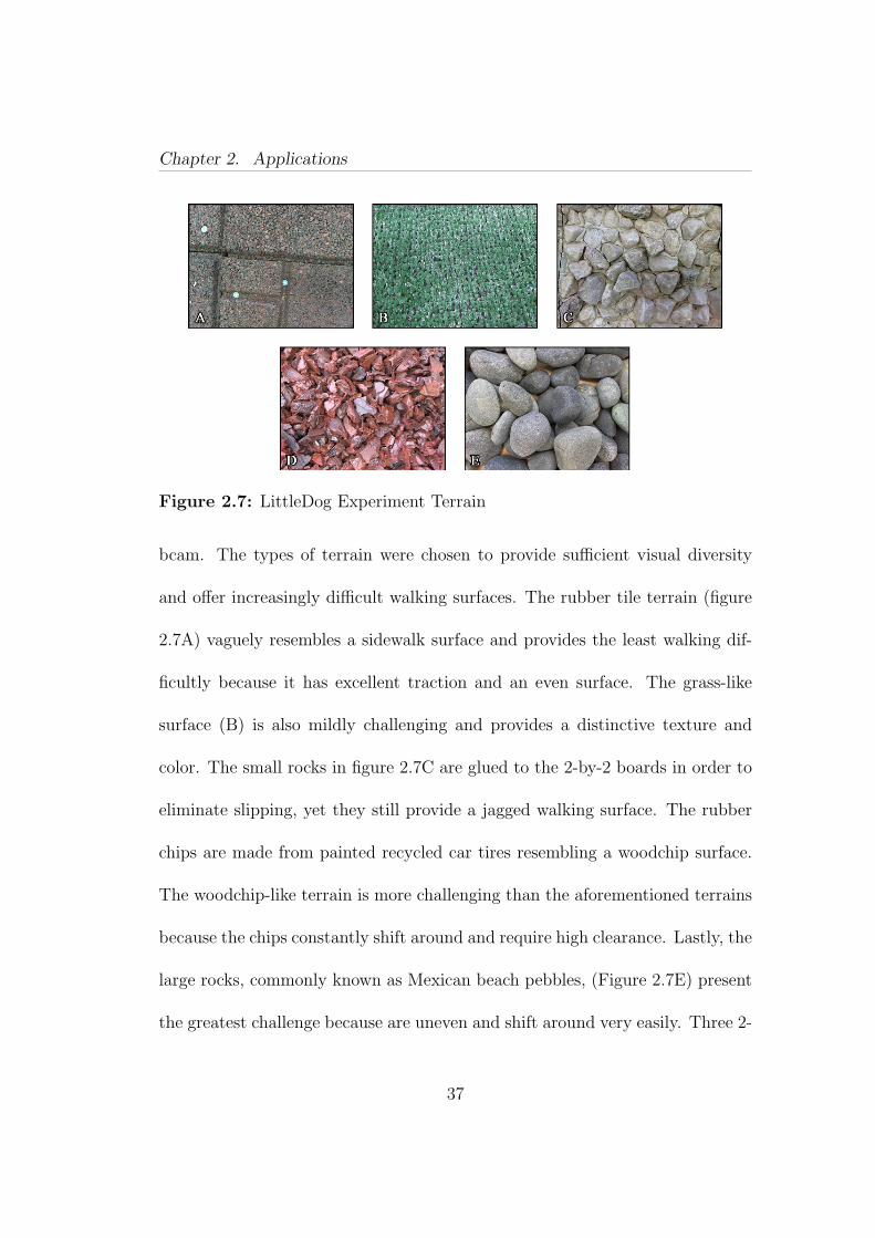
In order to create a controlled test environment several 2-by-2 foot terrain

boards/containers were created to mimic five natural terrain types. Figure 2.7

shows close-up images of each terrain type taken using the Logitech C910 we-

36


Figure 2.7: LittleDog Experiment Terrain

bcam. The types of terrain were chosen to provide sufficient visual diversity

and offer increasingly difficult walking surfaces. The rubber tile terrain (figure

2.7A) vaguely resembles a sidewalk surface and provides the least walking dif-

ficultly because it has excellent traction and an even surface. The grass-like

surface (B) is also mildly challenging and provides a distinctive texture and

color. The small rocks in figure 2.7C are glued to the 2-by-2 boards in order to

eliminate slipping, yet they still provide a jagged walking surface. The rubber

chips are made from painted recycled car tires resembling a woodchip surface.

The woodchip-like terrain is more challenging than the aforementioned terrains

because the chips constantly shift around and require high clearance. Lastly, the

large rocks, commonly known as Mexican beach pebbles, (Figure 2.7E) present

the greatest challenge because are uneven and shift around very easily. Three 2-

37


by-2 foot terrain boards were each created for the rubber tile, grass, and small

rocks. In order to test out a challenging loose terrain transition, the rubber

chips and large rocks were put into the same six-by-two foot container.

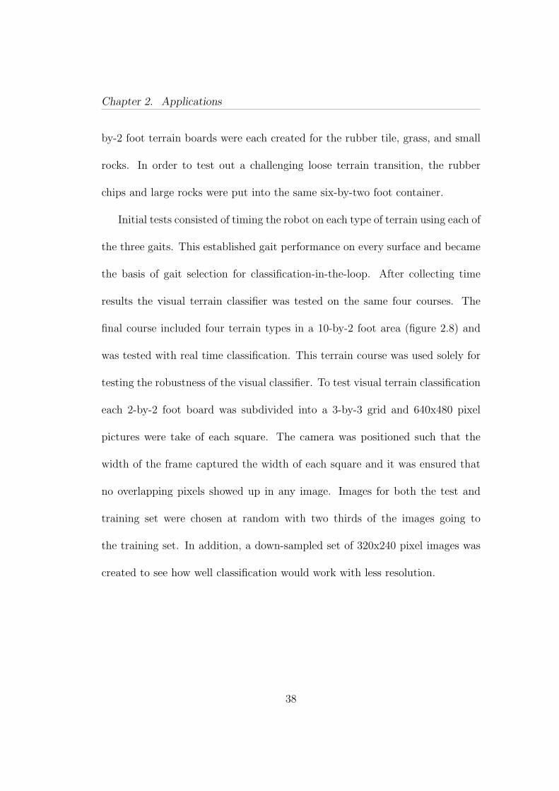
Initial tests consisted of timing the robot on each type of terrain using each of

the three gaits. This established gait performance on every surface and became

the basis of gait selection for classification-in-the-loop. After collecting time

results the visual terrain classifier was tested on the same four courses. The

final course included four terrain types in a 10-by-2 foot area (figure 2.8) and

was tested with real time classification. This terrain course was used solely for

testing the robustness of the visual classifier. To test visual terrain classification

each 2-by-2 foot board was subdivided into a 3-by-3 grid and 640x480 pixel

pictures were take of each square. The camera was positioned such that the

width of the frame captured the width of each square and it was ensured that

no overlapping pixels showed up in any image. Images for both the test and

training set were chosen at random with two thirds of the images going to

the training set. In addition, a down-sampled set of 320x240 pixel images was

created to see how well classification would work with less resolution.

38


Figure 2.8: LittleDog Traversing the Large Rocks Terrain Class

2.2.2 Results

Visually, each terrain is very distinct and offers a great deal of texture so we

did not foresee any problems during offline testing. Offline test results confirmed

that our experimental terrain was very well suited for classification and we were

able get 100% verification accuracy on both the 640x480 image set as well as

the 320x240 image set.Terrain

Small Rocks Big Rocks /Rubber Chips

Grass Rubber Tile

Gait B 22.0 DNC 20.8 20.7

C 27.7 29.3 26.4 25.8D 17.2 DNC 15.8 17.1

Classify 22.9 44.2 20.4 22.1

39


Gait D was designed to have very low ground clearance and a relatively fast

gait period, so naturally we expected it to perform well on grass and rubber tile.

We predicted that LittleDog would not be able to traverse the other terrains

because it would stub its feet against the protruding surfaces and veer off course.

This was not the case as illustrated by Table 2.2.2, and to the contrary gait D

performed the best on all terrain except for big rocks and rubber chips. On

the other extreme, our expectation was that Gait C would work reasonably well

for every terrain at the expense of speed. This was confirmed by our results,

and the only test that took more time was the classification trial for big rocks

/ rubber chips. We also predicted that Gait B, the hybrid gait, would perform

Small Rocks Chips/Big Rocks Grass Rubber Tile0

5

10

15

20

25

30

35

40

45

50

Gait C vs. Classification in the Loop Traversal Times

Tim

e (s

econ

ds)

All−Purpose Classification

Figure 2.9: Terrain Traversal Performance

40


the best on the small rock terrain due to its medium clearance and speed. Our

results determined that the hybrid gait was actually unnecessary since Gait D

performed faster on the small rock terrain.

Figure 2.9 shows a time comparison between Gait C and the classification

trial. Results indicate that classification was helpful in all cases except for the

most difficult terrain. Classification time was slower in that case due to the

stopping requirement. If this requirement did not exist, we would expect to see

a nearly identical time as Gait C.

Figure 2.10: Real Time Classification Results

During real time testing the camera auto-focus did not immediately react

to changes in object distance. LittleDog would, on occasion, tip the camera

downward during a stance and cause the picture to go slightly out of focus.

Image blurring decreases the performance of the fast Hessian feature detector

so we expected to see some misclassifications. Figure 2.10 shows a consecutive

41


classification trial that was performed on four types of terrain. Tests showed that

the classifier was in fact robust enough to minor image blurring (as demonstrated

by image 3), and in general there was a very low incidence of misclassifications.

2.3 Conclusion

We developed several novel algorithms that assist popular feature-based

recognition techniques. Feature extraction was improved with our gradient de-

scent inspired detection algorithm. Extracting a target number of features in-

creased classification accuracy while decreasing memory requirements. A sliding

window classifier was also designed to identify patches in heterogeneous terrain

images. This technique showed promising offline results, but struggled slightly

with terrain boundaries.

This work demonstrated the effectiveness of our feature-based terrain classi-

fication framework in offline and real-time testing. Offline experiments provided

valuable data on classification performance in a controlled environment. The

findings allowed us to select parameters that gave the most desirable mixture

of accuracy and performance. Real-time testing showed that our methods ef-

fectively aide autonomous navigation on the LittleDog platform. The robot

was able to traverse terrain faster with classification-in-the-loop despite requir-

42


ing stops to prevent camera blurring. The only case where this slowed the

robot was on the most difficult terrain which already required the slowest gait.

Overall, we demonstrated that our homogeneous classification approach can be

effectively used in real-time to aide quadruped navigation.

2.4 Future Work

This paper provides a solid terrain classification foundation for legged robots,

but there is an abundance of ideas to continue research. The primary goal of

this work was to create a proof of concept and as a result minimal effort was

spent on creating computationally efficient algorithms and code. The dynamic

feature adjuster is an example of an algorithm that can be recoded for efficiency.

The key point detection in the feature adjuster is computed from scratch at each

iteration, and perhaps calculations from the first iteration can be leveraged to

prevent further processing. In addition, most of the CPU intensive functions are

run in a sequential manner and do not utilize the parallel processing capabilities

of modern hardware. Many tasks, such as computing features for database

entries can be greatly sped up by dedicating concurrent computation threads.

The number of concurrent threads can be determined dynamically by looking

at the number of idle cores on the current CPU. In addition, there has been a

43


great deal of recent work on GPU-based computer vision libraries. This work

relies on several algorithms that can be processed on a GPU to drastically speed

up computation time.

The classification results in this work do not have any measure of confidence.

The SVM classifier can be used to produce such a confidence level or perhaps

the voting step in the sliding window method may be used to assign a measure

of agreement. This would simply involve looking at overlapping regions to de-

termine the amount of consensus among each classification result. On a broader

scale it would be interesting to try out different classification methods such as

boosting and artificial neural networks with the BOVW framework. A hybrid

classifier could also be used to combine color with features. It would also be

beneficial to compare our approach to popular terrain classification methods.

The work in [2] effectively uses textons to classify terrain in a very similar in

scope as this paper. Testing their algorithm using our terrain database would

give additional insight about the effectiveness of this work.

44

Bibliography

[1] Y. Alon, A. Ferencz, and A. Shashua. Off-road path following using regionclassification and geometric projection constraints. In Computer Visionand Pattern Recognition, pages 689–696, 2006.

[2] A. Angelova, L. Matthies, D. Helmick, and P. Perona. Fast terrain classifi-cation using variable-length representation for autonomous navigation. InComputer Vision and Pattern Recognition, 2007. CVPR ’07. IEEE Con-ference on, pages 1–8, June 2007.

[3] D. Arthur and S. Vassilvitskii. K-means++: the advantages of carefulseeding. Proc. of the 8th Annual ACM-SIAM Symposium on Discrete Al-gorithms, pages 1027–1035, 2007.

[4] H. Bay, T. Tuytelaars, and L. V. Gool. Surf: Speeded up robust features.In Proceedings of the ninth European Conference on Computer Vision, May2006.

[5] C. Brooks and K. Iagnemma. Vibration-based terrain classification forplanetary exploration rovers. Robotics, IEEE Transactions on, 21(6):1185– 1191, dec. 2005.

[6] Y. Cheng, M. Maimone, and L. Matthies. Visual odometry on the marsexploration rovers - a tool to ensure accurate driving and science imaging.Robotics Automation Magazine, IEEE, 13(2):54 –62, june 2006.

[7] A. Chilian and H. Hirschmuller. Stereo camera based navigation of mobilerobots on rough terrain. Intelligent Robots and Systems, pages 4571–4576,2009.

[8] J. D. Crisman and C. E. Thorpe. Color vision for road following. In Visionand Navigation: The CMU Navlab, C. Thorpe (Ed, pages 9–24. KluwerAcademic Publishers, 1988.

45

Bibliography

[9] G. Csurka, C. R. Dance, L. Fan, J. Willamowski, and C. Bray. Visualcategorization with bags of keypoints. In Workshop on Statistical Learningin Computer Vision, ECCV, pages 1–22, 2004.

[10] T. Deselaers, L. Pimenidis, and H. Ney. Bag-of-visual-words models foradult image classification and filtering. In Pattern Recognition, 2008. ICPR2008. 19th International Conference on, pages 1–4, dec. 2008.

[11] S. Gammeter, L. Bossard, T. Quack, and L. V. Gool. I know what you didlast summer: object-level auto-annotation of holiday snaps. InternationalConf. on Computer Vision, 2009.

[12] C.-W. Hsu, C.-C. Chang, and C.-J. Lin. A practical guide to support vec-tor classification. http://www.csie.ntu.edu.tw/~cjlin/papers/guide/guide.pdf, 2003.

[13] X. Liu and D. Wang. Texture classification using spectral histograms. IEEETransactions on Image Processing, 12:661–669, 2003.

[14] D. G. Lowe. Object recognition from local scale-invariant features. Inter-national Conf. on Computer Vision, 1999.

[15] M. Luetzeler and S. Baten. Road recognition for a tracked vehicle. Proc.SPIE Enhanced and Synthetic Vision, 4023(1):171–180, 2000.

[16] R. Manduchi, A. Castano, A. Talukder, and L. Matthies. Obstacle de-tection and terrain classification for autonomous off-road navigation. Au-tonomous Robots, 18:81–102, 2004.

[17] C. Manning and H. Schutze. Foundations of Statistical Natural LanguageProcessing. MIT Press, May 1999.

[18] D. Nister and H. Stewenius. Scalable recognition with a vocabulary tree.In IN CVPR, pages 2161–2168, 2006.

[19] J. Philbin, O. Chum, M. Isard, J. Sivic, and A. Zisserman. Object retrievalwith large vocabularies and fast spatial matching. In Computer Vision andPattern Recognition, 2007. CVPR ’07. IEEE Conference on, pages 1–8,june 2007.

[20] A. Pretto, E. Menegatti, and E. Pagello. Reliable features matching forhumanoid robots. In Humanoid Robots, 2007 7th IEEE-RAS InternationalConference on, pages 532 –538, 29 2007-dec. 1 2007.

46

Bibliography

[21] N. Sebe, M. S. Lew, and N. Bohrweg. Wavelet based texture classification.In in International Conference on Pattern Recognition, 2000, pages 959–962, 2000.

[22] M. Singh and S. Singh. Spatial texture analysis: a comparative study. InPattern Recognition, 2002. Proceedings. 16th International Conference on,volume 1, pages 676 – 679 vol.1, 2002.

[23] S. Thrun, M. Montemerlo, H. Dahlkamp, D. Stavens, and et. al. The robotthat won the darpa grand challenge. Journal of Field Robotics, 23:661–692,2006.

[24] J. S. Weszka, C. R. Dyer, and A. Rosenfeld. A comparative study of texturemeasures for terrain classification. Systems, Man and Cybernetics, IEEETransactions on, SMC-6(4):269 –285, april 1976.

47

Visual Terrain Classi cation For Legged Robotskatiebyl/papers/Filitchkin_MSThesis.pdfterrain images...

Documents

Transcript of Visual Terrain Classi cation For Legged Robotskatiebyl/papers/Filitchkin_MSThesis.pdfterrain images...