Visual Exploration of Patterns in Multi-run Time-varyingMulti-field Simulation Data Using Projected Views

Vladimir MolchanovJacobs UniversityCampus Ring 1

28759 Bremen, Germanyv.molchanov@jacobs-university.de

Lars LinsenJacobs UniversityCampus Ring 1

28759 Bremen, Germanyl.linsen@jacobs-university.de

ABSTRACTIn the fields of science and engineering, it is common to run hundreds of simulations to investigate the dependenceof the modeled process on various simulation and input the parameters. We propose a comprehensive approachfor the visual analysis of such multi-run data to detect patterns and outliers. We use dimensionality reductionalgorithms to generate a visual representation that exhibits the distribution of the simulation results under varyingparameter settings. Each field (or even multi-field) of every time step and every simulation run is representedas a point in a 2D space, where the 2D layout conveys similarity of the scalar fields. Points corresponding toconsecutive time steps of one run are connected by line segments, such that each simulation run is represented as apolyline. Consequently, the multi-run data are visually encoded as a set of polylines. Variations of hue, saturation,opacity, and shape allow for distinguishing groups of simulations and depicting various characteristics of runs. Theuser can interactively change these settings, while further interaction mechanisms allow for selection, refinement,zooming, requesting textual information, and brushing and linking to coordinated (or embedded) views of physicaland attribute space visualizations. We apply our approach to two applications with significantly different datastructure: a multi-run climate simulation over a 2D regular grid and a multi-run binary star evolution simulationwith unstructured 3D particles evolving over time. We demonstrate the contribution and impact of our visualizationmethod for the interactive visual analysis of the multi-run data by identifying meaningful groups of simulations,detecting global patterns, and finding interesting outliers.

KeywordsTime-varying Data, Multi-field, Multi-modal and Multi-variate Data, Scalar Field Data, Dimensionality Reduction

1 INTRODUCTION

Multi-run (or ensemble) simulations in the fields of sci-ence and engineering serve to investigate dependenceof modeled time-varying phenomena on various simu-lation and input parameters. Typical goals when gener-ating and analyzing multi-run simulations are to explorethe entire space of possible scenarios, to find optimal orto detect critical parameter settings, and to investigatehow sensitive outputs are to certain input parameters.Obviously, a large number of simulations need to beperformed in order to obtain a sufficiently dense pa-rameter space sampling. The analysis of the resultingdatasets is extremely challenging, since the data oftendescribe time-varying multi-fields, which when com-

Permission to make digital or hard copies of all or part ofthis work for personal or classroom use is granted withoutfee provided that copies are not made or distributed for profitor commercial advantage and that copies bear this notice andthe full citation on the first page. To copy otherwise, or re-publish, to post on servers or to redistribute to lists, requiresprior specific permission and/or a fee.

puted for multiple runs quickly reach extremely largesizes.Novel visualization approaches can be very helpfulfor researches to simplify post-processing of multi-rundatasets. This stage may include fast navigation overthe data, selection of an individual simulation (or atime step) or a subset thereof for detailed comparison,visual encoding of various characteristics of runs, andeasy creation of animations. However, the first stepafter the dataset is generated is to throw a glance at thedataset in order to roughly estimate its homogeneity,to build a notion of a typical simulation behavior(common pattern) and to identify those simulationswhose behavior significantly differs from the pattern(outliers). We propose a technique to produce anoverview representation of a complete multi-rundataset, equip it with a number of interaction toolsbased on coordinated views, and demonstrate theeffectiveness of the resulting system on two applicationexamples.The proposed framework for interactive visual analy-sis of multi-run data is based on coordinated views ofnumerous aspects of multi-run data. Pattern and out-

lier detection in multi-run simulations is supported by aprojected view of an attribute space. The attribute spaceis derived from the data space by defining characteristicproperties of a simulation time step. According to thatattribute space representation of each time step of eachsimulation run, we compare different time steps of thesame or different simulation runs with each other. Wecreate a 2D layout that depicts similarity or dissimilar-ity of time steps using dimension reduction methods.Each time step is represented as a point in this 2D lay-out and runs are shown as polylines connecting thosepoints. In such a layout, runs of similar behavior have asimilar polyline trajectory. Hence, patterns can be ob-served quickly and the same is true for trajectories thatdo not adhere to the pattern, i.e., outliers.

Although this similarity view is most important for an-alyzing multiple simulation runs, it is equally impor-tant that one can relate detected outliers or otherwiseinteresting runs to the parameter space and the multi-ple fields that are simulated. Our framework is basedon coordinated views of parameter space visualization,spatial data visualization of the fields, visualization ofthe derived attribute space, and the projected views.

We present the overall framework of our work (Sec-tion 3) and demonstrate its effectiveness and intuitive-ness by deploying it to two rather different instances(Section 4). The first instance is a grid-based climatesimulation, where the attribute space can be triviallyderived from the data space and the derived projectionpatterns follow our intuition. The second instance isa particle-based astrophysical simulation, where a non-trivial computation of the attribute space was necessaryand where we show how our framework allows for in-teractive analysis of multi-run data. In this context, wealso apply multiple coordinated projected views.

2 RELATED WORKBesides a constant grow of size of generated and reg-istered scientific data, their increasing complexity andheterogeneity becomes a hot topic in modern researchesin the field of data mining and visualization. Kehrer andHauser [KH13] wrote recently a survey on visualizationmethods for multi-faceted data. Multi-faceted is here ageneral term to emphasize the fact, that scientific datamay have spatio-temporal structure and/or multi-variateformat, may consist of parts stemming from differentmodalities, may be multi-run and/or multi-model data.

User interaction plays a crucial role when inspectingthe interplay of initial conditions and simulation results.Brushing and linking embedded into a coordinated mul-tiple views framework is probably the most popular toolin visualization systems aimed to handle multi-run data.Examples of interactive exploration of parameter spacecan be found in [MAB+97, Ma99, MOD00, SPK+07].

Pattern recognition and annotation of clusters and out-liers can be helpful for researchers leading multi-runsimulations in order to plan further tests, re-sample pa-rameter space to obtain detailed local information anddefine critical parameter settings. A recent grid-densitybased technique to complete these tasks was proposedby Kandogan [Kan12].

Supporting uncertainty in the visual analytics processis of great importance in systems aimed to help the userto find optimal parameter settings. A framework for un-certainty modeling, propagation and aggregation is pro-posed by Correa et al. [CCM09]. Possible solutions forgraphical representation of uncertainty are discussed inCooke and Noortwijk [CvN00].

Bruckner and Möller [BM10] developed a visualizationsystem helping the user to find simulation parameterscorresponding to the desired outcome animation. Theirapproach is based on a spatio-temporal clustering tech-nique producing an overview of achievable final statesand their trajectories in the phase space. Another novelapproach for mapping of deforming mesh sequencesto the visual domain is given by Cashman and Hor-mann [CH12]. The user is allowed, in particular, tocreate an arbitrarily-shaped path in the abstract repre-sentation domain, from which a corresponding meshanimation can be reconstructed.

We are the first who developed a framework for ana-lyzing multi-run time-varying multi-field data. In ourwork, we propose to use dimensionality reduction al-gorithms [JJ09] including the classical Principle Com-ponent Analysis (PCA) [Pea01] and MultidimensionalScaling (MDS) [BG05] to produce 2D similarity lay-outs between time steps of multiple simulation runs.This set-up allows for an interactive visual detection ofpatterns and outliers in the multi-run data, especiallywhen embedded in our coordinated views frameworkof parameter space visualization, spatial data visualiza-tion, and visualization of a derived attribute space inaddition to the projected view visualization.

3 INTERACTIVE VISUAL ANALYSISFRAMEWORK

Multi-run data result from a repeating procedure ofpicking an instance from the parameter space PS andrunning a simulation for selected input parameters. Foreach chosen set of parameters, the simulation typicallycreates a time-varying multi-field data set, i.e., a spa-tial phenomenon is simulated using a multitude of fieldsthat change over time. To effectively capture or samplethe parameter space, the simulation has to be run manytimes for different initial conditions (or parameter set-tings). As a result, one obtains a large amount of time-varying multi-field simulation results. When changingthe parameter setting, the simulation result changes in

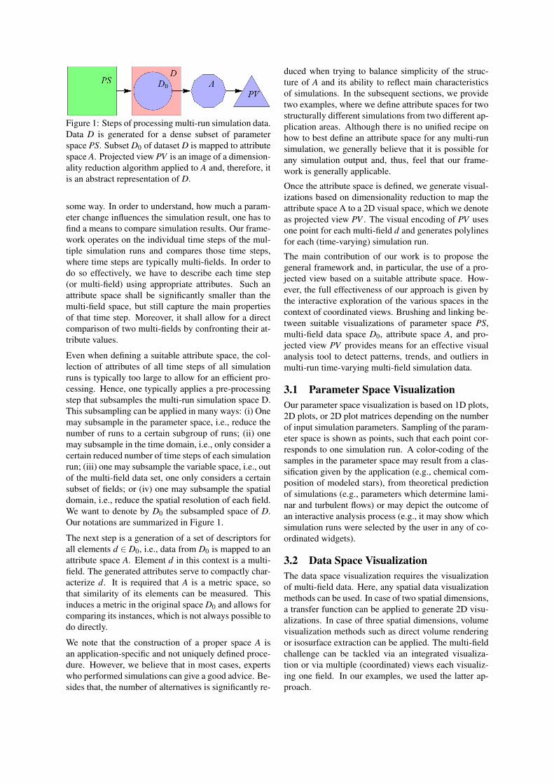
Figure 1: Steps of processing multi-run simulation data.Data D is generated for a dense subset of parameterspace PS. Subset D0 of dataset D is mapped to attributespace A. Projected view PV is an image of a dimension-ality reduction algorithm applied to A and, therefore, itis an abstract representation of D.

some way. In order to understand, how much a param-eter change influences the simulation result, one has tofind a means to compare simulation results. Our frame-work operates on the individual time steps of the mul-tiple simulation runs and compares those time steps,where time steps are typically multi-fields. In order todo so effectively, we have to describe each time step(or multi-field) using appropriate attributes. Such anattribute space shall be significantly smaller than themulti-field space, but still capture the main propertiesof that time step. Moreover, it shall allow for a directcomparison of two multi-fields by confronting their at-tribute values.

Even when defining a suitable attribute space, the col-lection of attributes of all time steps of all simulationruns is typically too large to allow for an efficient pro-cessing. Hence, one typically applies a pre-processingstep that subsamples the multi-run simulation space D.This subsampling can be applied in many ways: (i) Onemay subsample in the parameter space, i.e., reduce thenumber of runs to a certain subgroup of runs; (ii) onemay subsample in the time domain, i.e., only consider acertain reduced number of time steps of each simulationrun; (iii) one may subsample the variable space, i.e., outof the multi-field data set, one only considers a certainsubset of fields; or (iv) one may subsample the spatialdomain, i.e., reduce the spatial resolution of each field.We want to denote by D0 the subsampled space of D.Our notations are summarized in Figure 1.

The next step is a generation of a set of descriptors forall elements d ∈ D0, i.e., data from D0 is mapped to anattribute space A. Element d in this context is a multi-field. The generated attributes serve to compactly char-acterize d. It is required that A is a metric space, sothat similarity of its elements can be measured. Thisinduces a metric in the original space D0 and allows forcomparing its instances, which is not always possible todo directly.

We note that the construction of a proper space A isan application-specific and not uniquely defined proce-dure. However, we believe that in most cases, expertswho performed simulations can give a good advice. Be-sides that, the number of alternatives is significantly re-

duced when trying to balance simplicity of the struc-ture of A and its ability to reflect main characteristicsof simulations. In the subsequent sections, we providetwo examples, where we define attribute spaces for twostructurally different simulations from two different ap-plication areas. Although there is no unified recipe onhow to best define an attribute space for any multi-runsimulation, we generally believe that it is possible forany simulation output and, thus, feel that our frame-work is generally applicable.

Once the attribute space is defined, we generate visual-izations based on dimensionality reduction to map theattribute space A to a 2D visual space, which we denoteas projected view PV . The visual encoding of PV usesone point for each multi-field d and generates polylinesfor each (time-varying) simulation run.

The main contribution of our work is to propose thegeneral framework and, in particular, the use of a pro-jected view based on a suitable attribute space. How-ever, the full effectiveness of our approach is given bythe interactive exploration of the various spaces in thecontext of coordinated views. Brushing and linking be-tween suitable visualizations of parameter space PS,multi-field data space D0, attribute space A, and pro-jected view PV provides means for an effective visualanalysis tool to detect patterns, trends, and outliers inmulti-run time-varying multi-field simulation data.

3.1 Parameter Space VisualizationOur parameter space visualization is based on 1D plots,2D plots, or 2D plot matrices depending on the numberof input simulation parameters. Sampling of the param-eter space is shown as points, such that each point cor-responds to one simulation run. A color-coding of thesamples in the parameter space may result from a clas-sification given by the application (e.g., chemical com-position of modeled stars), from theoretical predictionof simulations (e.g., parameters which determine lami-nar and turbulent flows) or may depict the outcome ofan interactive analysis process (e.g., it may show whichsimulation runs were selected by the user in any of co-ordinated widgets).

3.2 Data Space VisualizationThe data space visualization requires the visualizationof multi-field data. Here, any spatial data visualizationmethods can be used. In case of two spatial dimensions,a transfer function can be applied to generate 2D visu-alizations. In case of three spatial dimensions, volumevisualization methods such as direct volume renderingor isosurface extraction can be applied. The multi-fieldchallenge can be tackled via an integrated visualiza-tion or via multiple (coordinated) views each visualiz-ing one field. In our examples, we used the latter ap-proach.

3.3 Attribute Space VisualizationAs mentioned above, the definition of the attributespace is application-specific. Its visualization dependson the respective choice made within the application.In some cases, attribute space visualization can beembedded in the projected view (e.g, in form ofpictograms) to allow visual correlation of the projectedview layout with descriptive attributes.

3.4 Projected View VisualizationAfter data subset D0 is mapped to attribute space, it canbe projected to the visual domain of the projected viewbased on dissimilarities of the elements in A. Again, itdepends on the choice of attribute space A, which pro-jection method is most suitable. We want to providesome guidelines: If A is isomorphic to an Euclideanspace, the range of available methods is large and in-cludes such algorithms as PCA. Otherwise, if only dis-similarity measures can be computed, good candidatesare MDS, SPE, PLMP and their variants. The choice ofa proper method should be based on two main criteria:First, efficiency of the algorithm should allow for fastprocessing of large data, and second, similarity of pro-jected elements should be conserved as much as pos-sible. The latter criterion means that the distribution ofsamples in attribute space shall be matched as closely aspossible in the projected view. Besides that, if the algo-rithm constructs a projection operator in explicit form,it is possible to apply it later to the whole dataset D.This is, in particular, the case if the projection acts as alinear operator.

An image of D0 on the projected view is a set of points,each representing a certain time step of a simulationfrom the dataset. Since it makes sense to analyse simu-lation trajectories rather than separated time steps, it ishelpful to connect points representing consecutive timesteps from the same simulation run by line segments.

Based on shape and location of the drawn trajectories,it can be easily observed, which simulation runs behavesimilarly. This facilitates detecting patterns and generaltrends. Moreover, outliers can be identified, where out-lier detection relates to both finding trajectories follow-ing abnormal or remarkable paths and single extremenodes denoting special states of the system. We wantto note that outliers, if any, may refer to a phenomenondetected for a special parameter setting as well as to thesettings, for which the underlying physical model be-comes invalid or applied numerical methods fail.

3.5 Interaction and Coordinated ViewsAll four views on the data contribute unique informa-tion about the multi-run simulation. Most effective arethey, if they are coordinated such that any selectionsmade in one view are shown and can be further refinedin all the other views. As such, one can, for example,

detect and select outliers in the projected view, investi-gate which parameter settings they relate to in the pa-rameter space visualization, select a subset of the out-liers by brushing in the parameter space, investigate re-spective time steps of that run in the data space visu-alization, and relate them to the attributes space to ob-serve what attributes made them to be outliers.

Moreover, one may generate multiple attribute spacesper element d ∈D0, e.g., one per data field. Then, mul-tiple projected views are generated and coordination ofthese views allows for interactive analysis of runs withrespective to different fields. Examples are given in thesubsequent sections. The effectiveness of the coordi-nated interaction is best observed in the accompanyingvideo.

We also provide further interaction mechanisms withthe projected views. When investigating many runs ormany time steps simultaneously, opening too many co-ordinated views may become confusing at some point.To provide a better overview of which point of the pro-jected view belongs to which kind of observed phe-nomena, we provide embedded views of data or at-tribute space visualizations as shown in Figure 2. Theuser may enable an option of showing small pictogramsnear selected points characterizing the current state ofthe system (Figure 2a). Here, the pictograms are low-resolution visualizations of the attribute space with auser-defined transfer function applied. We used thesame color scheme in all renderings of data or attributespaces, see Figure 2c. In addition, a textual informationabout a single selected element is shown in the lower-left corner of the screen. This textual information pro-vides the necessary information for the user to uniquelyidentify the run and time step that is under investiga-tion. Moreover, the trajectories in the projected vieware color coded. The user may choose, which infor-mation is color coded, e.g., showing a given classifica-tion (Figure 2a) or assigning to every simulation gets adifferent color. However, since the number of simula-tions is typically large, there is the perceptual issue thathumans can only distinguish well a certain amount ofcolors with different hues. Therefore, if a group of tra-jectories is selected, it is possible to redistribute colorsamong these elements to better distinguish individualtrajectories (Figure 2b).

4 INSTANCES OF FRAMEWORKWe produce two instances of our general framework byapplying our technique to two datasets of very differentstructure. The first one represents a 100-year time seriesof a quasi-equilibrated (“persisting”) preindustrial cli-mate state. The data are sampled on a 2D regular grid,which makes the construction of attribute space trivial.We process these easy-to-handle data to illustrate howintuitively expectations match with the projected view

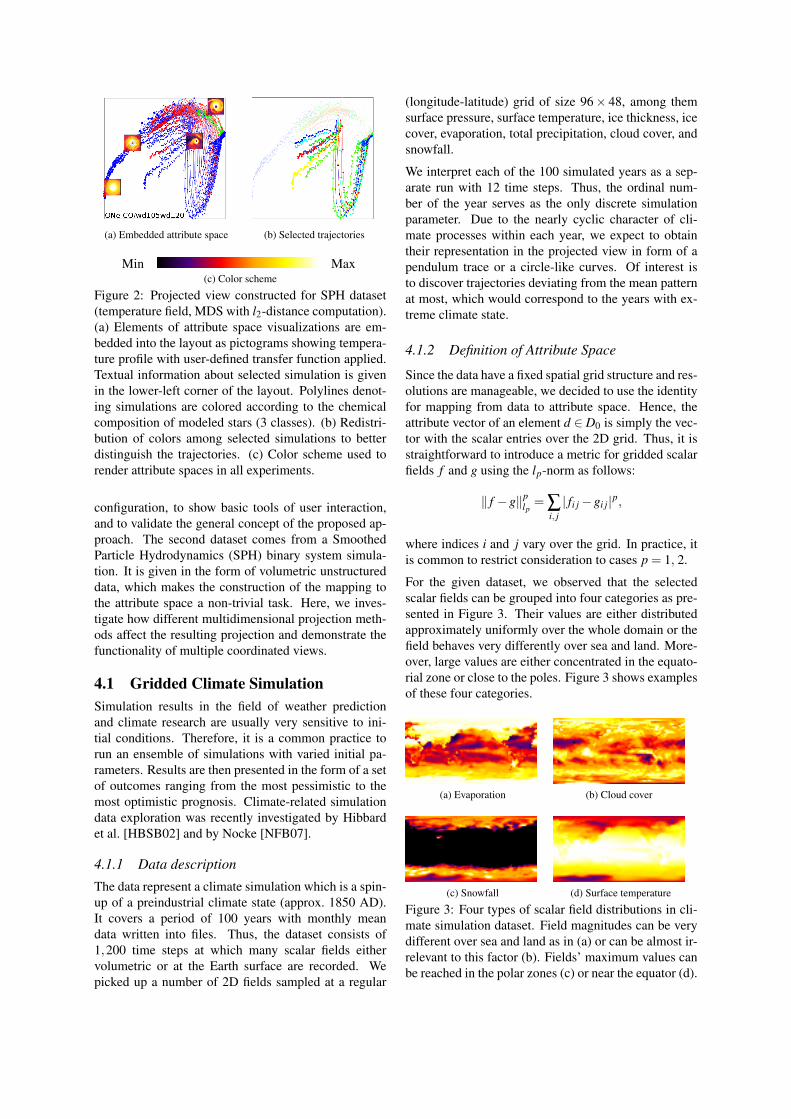
(a) Embedded attribute space (b) Selected trajectories

Min Max(c) Color scheme

Figure 2: Projected view constructed for SPH dataset(temperature field, MDS with l2-distance computation).(a) Elements of attribute space visualizations are em-bedded into the layout as pictograms showing tempera-ture profile with user-defined transfer function applied.Textual information about selected simulation is givenin the lower-left corner of the layout. Polylines denot-ing simulations are colored according to the chemicalcomposition of modeled stars (3 classes). (b) Redistri-bution of colors among selected simulations to betterdistinguish the trajectories. (c) Color scheme used torender attribute spaces in all experiments.

configuration, to show basic tools of user interaction,and to validate the general concept of the proposed ap-proach. The second dataset comes from a SmoothedParticle Hydrodynamics (SPH) binary system simula-tion. It is given in the form of volumetric unstructureddata, which makes the construction of the mapping tothe attribute space a non-trivial task. Here, we inves-tigate how different multidimensional projection meth-ods affect the resulting projection and demonstrate thefunctionality of multiple coordinated views.

4.1 Gridded Climate SimulationSimulation results in the field of weather predictionand climate research are usually very sensitive to ini-tial conditions. Therefore, it is a common practice torun an ensemble of simulations with varied initial pa-rameters. Results are then presented in the form of a setof outcomes ranging from the most pessimistic to themost optimistic prognosis. Climate-related simulationdata exploration was recently investigated by Hibbardet al. [HBSB02] and by Nocke [NFB07].

4.1.1 Data description

The data represent a climate simulation which is a spin-up of a preindustrial climate state (approx. 1850 AD).It covers a period of 100 years with monthly meandata written into files. Thus, the dataset consists of1,200 time steps at which many scalar fields eithervolumetric or at the Earth surface are recorded. Wepicked up a number of 2D fields sampled at a regular

(longitude-latitude) grid of size 96× 48, among themsurface pressure, surface temperature, ice thickness, icecover, evaporation, total precipitation, cloud cover, andsnowfall.

We interpret each of the 100 simulated years as a sep-arate run with 12 time steps. Thus, the ordinal num-ber of the year serves as the only discrete simulationparameter. Due to the nearly cyclic character of cli-mate processes within each year, we expect to obtaintheir representation in the projected view in form of apendulum trace or a circle-like curves. Of interest isto discover trajectories deviating from the mean patternat most, which would correspond to the years with ex-treme climate state.

4.1.2 Definition of Attribute Space

Since the data have a fixed spatial grid structure and res-olutions are manageable, we decided to use the identityfor mapping from data to attribute space. Hence, theattribute vector of an element d ∈D0 is simply the vec-tor with the scalar entries over the 2D grid. Thus, it isstraightforward to introduce a metric for gridded scalarfields f and g using the lp-norm as follows:

‖ f −g‖plp= ∑

i, j| fi j−gi j|p,

where indices i and j vary over the grid. In practice, itis common to restrict consideration to cases p = 1, 2.

For the given dataset, we observed that the selectedscalar fields can be grouped into four categories as pre-sented in Figure 3. Their values are either distributedapproximately uniformly over the whole domain or thefield behaves very differently over sea and land. More-over, large values are either concentrated in the equato-rial zone or close to the poles. Figure 3 shows examplesof these four categories.

(a) Evaporation (b) Cloud cover

(c) Snowfall (d) Surface temperature

Figure 3: Four types of scalar field distributions in cli-mate simulation dataset. Field magnitudes can be verydifferent over sea and land as in (a) or can be almost ir-relevant to this factor (b). Fields’ maximum values canbe reached in the polar zones (c) or near the equator (d).

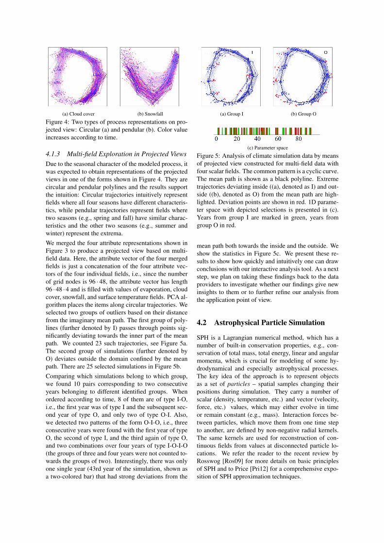
(a) Cloud cover (b) Snowfall

Figure 4: Two types of process representations on pro-jected view: Circular (a) and pendular (b). Color valueincreases according to time.

4.1.3 Multi-field Exploration in Projected ViewsDue to the seasonal character of the modeled process, itwas expected to obtain representations of the projectedviews in one of the forms shown in Figure 4. They arecircular and pendular polylines and the results supportthe intuition: Circular trajectories intuitively representfields where all four seasons have different characteris-tics, while pendular trajectories represent fields wheretwo seasons (e.g., spring and fall) have similar charac-teristics and the other two seasons (e.g., summer andwinter) represent the extrema.

We merged the four attribute representations shown inFigure 3 to produce a projected view based on multi-field data. Here, the attribute vector of the four mergedfields is just a concatenation of the four attribute vec-tors of the four individual fields, i.e., since the numberof grid nodes is 96 · 48, the attribute vector has length96 ·48 ·4 and is filled with values of evaporation, cloudcover, snowfall, and surface temperature fields. PCA al-gorithm places the items along circular trajectories. Weselected two groups of outliers based on their distancefrom the imaginary mean path. The first group of poly-lines (further denoted by I) passes through points sig-nificantly deviating towards the inner part of the meanpath. We counted 23 such trajectories, see Figure 5a.The second group of simulations (further denoted byO) deviates outside the domain confined by the meanpath. There are 25 selected simulations in Figure 5b.

Comparing which simulations belong to which group,we found 10 pairs corresponding to two consecutiveyears belonging to different identified groups. Whenordered according to time, 8 of them are of type I-O,i.e., the first year was of type I and the subsequent sec-ond year of type O, and only two of type O-I. Also,we detected two patterns of the form O-I-O, i.e., threeconsecutive years were found with the first year of typeO, the second of type I, and the third again of type O,and two combinations over four years of type I-O-I-O(the groups of three and four years were not counted to-wards the groups of two). Interestingly, there was onlyone single year (43rd year of the simulation, shown asa two-colored bar) that had strong deviations from the

(a) Group I (b) Group O

(c) Parameter space

Figure 5: Analysis of climate simulation data by meansof projected view constructed for multi-field data withfour scalar fields. The common pattern is a cyclic curve.The mean path is shown as a black polyline. Extremetrajectories deviating inside ((a), denoted as I) and out-side ((b), denoted as O) from the mean path are high-lighted. Deviation points are shown in red. 1D parame-ter space with depicted selections is presented in (c).Years from group I are marked in green, years fromgroup O in red.

mean path both towards the inside and the outside. Weshow the statistics in Figure 5c. We present these re-sults to show how quickly and intuitively one can drawconclusions with our interactive analysis tool. As a nextstep, we plan on taking these findings back to the dataproviders to investigate whether our findings give newinsights to them or to further refine our analysis fromthe application point of view.

4.2 Astrophysical Particle Simulation

SPH is a Lagrangian numerical method, which has anumber of built-in conservation properties, e.g., con-servation of total mass, total energy, linear and angularmomenta, which is crucial for modeling of some hy-drodynamical and especially astrophysical processes.The key idea of the approach is to represent objectsas a set of particles – spatial samples changing theirpositions during simulation. They carry a number ofscalar (density, temperature, etc.) and vector (velocity,force, etc.) values, which may either evolve in timeor remain constant (e.g., mass). Interaction forces be-tween particles, which move them from one time stepto another, are defined by non-negative radial kernels.The same kernels are used for reconstruction of con-tinuous fields from values at disconnected particle lo-cations. We refer the reader to the recent review byRosswog [Ros09] for more details on basic principlesof SPH and to Price [Pri12] for a comprehensive expo-sition of SPH approximation techniques.

4.2.1 Data DescriptionThe dataset consists of simulations’ outputs of themerger process of two White Dwarfs (WD). Thestars are bound by gravity, which triggers a masstransfer from the lighter star (donor) to the heavier one(accretor). This process affects the orbital evolution,the angular momentum and the thermodynamical stateof the final object, the associated gravity wave signal,and whether or not a particular binary merges at all.Simulation of binary systems is of great importancein astrophysics, see, for example, grid- [MFTD07]and particle-based simulations [DRGRR11]. In thegrid-based calculations, the mass transfer continues fortens of orbits, whereas particle simulations showed thatthe stars merge after a few orbital periods. This led todiscussions about impact of accurate initial conditionson the stability of the modeled process.

The main input parameters are the masses of donor andaccretor stars, denoted by M1 and M2 (M1 ≤ M2), cor-respondingly. The main goals of the study are:

• understand the evolution of WD systems from theonset of mass transfer until the merger,

• identify accurately the parameter space regionwhere detonations may occur in the lead-up to themerger or at surface contact,

• compare against previous SPH and grid-based cal-culations, in particular, examine the duration of sta-ble mass transfer phase.

Both M1 and M2 (measured in units of the solar mass)take real values. It is assumed that the simulation outputcontinuously depends on the governing parameters.

The available part of the dataset consisting of 78 sim-ulations can be classified according to the chemicalcomposition of WDs: double Carbon-Oxygen (CO-CO), double Helium-Carbon-Oxygen (HeCO-HeCO),and Oxygen-Neon / Carbon-Oxygen (ONe-CO) bina-ries, see Figure 6a. Every simulation involves 40k par-ticles (20k particles for each star) and includes two vec-tor fields (velocity and gravity), six scalar fields (parti-cle radius, internal energy, mass, density, temperature,and electron density), and many chemical units records.The simulations are stopped after a timescale of morethan three initial orbital periods from the merger mo-menta, which results in different number of time stepsfor different simulations ranging from 600 to 1,600.The total size of the dataset exceeds 0.5TB.

4.2.2 Choosing Data SpaceTo build up a representative subset D0 of the whole data,which is possible to operate in reasonable time, we tookevery tenth recorded time step from each simulation andskipped the part of data related to chemical componentsof stars. The resulting data consist of 6,231 time stepstaking 32GB of disk space.

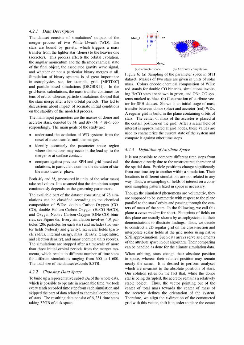
(a) Parameter space (b) Attributes computation

Figure 6: (a) Sampling of the parameter space in SPHdataset. Masses of two stars are given in units of solarmass. Colors encode chemical composition of WDs:red stands for double CO binaries, simulations involv-ing HeCO stars are shown in green, and ONe-CO sys-tems marked as blue. (b) Construction of attribute vec-tor for SPH dataset. Shown is an initial stage of masstransfer between donor (blue) and accretor (red) WDs.A regular grid is build in the plane containing orbits ofstars. The center of mass of the accretor is placed atthe certain position on the grid. After a scalar field ofinterest is approximated at grid nodes, these values areused to characterize the current state of the system andcompare it against other time steps.

4.2.3 Definition of Attribute Space

It is not possible to compare different time steps fromthe dataset directly due to the unstructured character ofthe spatial data. Particle positions change significantlyfrom one time step to another within a simulation. Theirlocations in different simulations are not related in anyway. Thus, a re-sampling of fields of interest on a com-mon sampling pattern fixed in space is necessary.

Though the simulated phenomena are volumetric, theyare supposed to be symmetric with respect to the planeparallel to the stars’ orbits and passing through the cen-ters of mass of the stars. In the following, we call thisplane a cross-section for short. Footprints of fields onthis plane are usually shown by astrophysicists in theirdemonstrations to illustrate findings. Thus, we decideto construct a 2D regular grid on the cross-section andinterpolate scalar fields at the grid nodes using nativeSPH approximation. Such data arrays serve as elementsof the attribute space in our algorithm. Their comparingcan be handled as done for the climate simulation data.

When orbiting, stars change their absolute positionin space, whereas their relative position may remainnearly the same. It is desired to perform analyseswhich are invariant to the absolute positions of stars.Our solution relies on the fact that, while the donorstar is being disrupted, the accretor remains a relativelystable object. Thus, the vector pointing out of thecenter of total mass towards the center of mass ofthe accretor defines the orientation of the system.Therefore, we align the x-direction of the constructedgrid with this vector, shift it in order to place the center

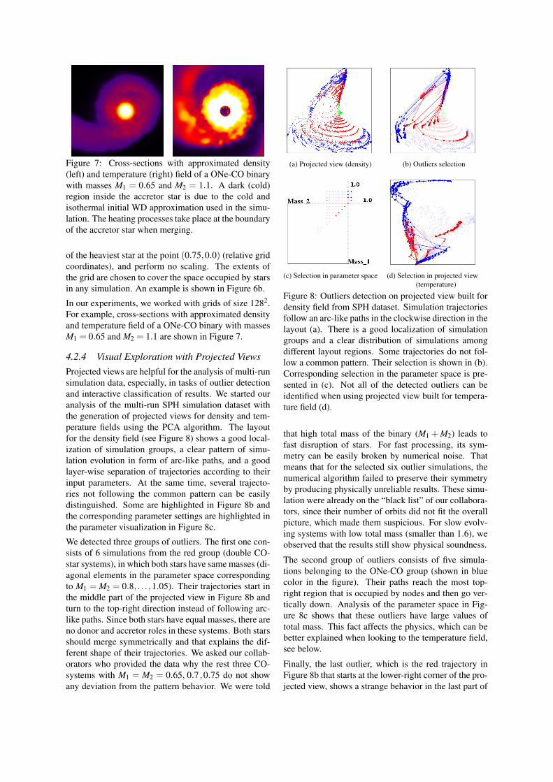
Figure 7: Cross-sections with approximated density(left) and temperature (right) field of a ONe-CO binarywith masses M1 = 0.65 and M2 = 1.1. A dark (cold)region inside the accretor star is due to the cold andisothermal initial WD approximation used in the simu-lation. The heating processes take place at the boundaryof the accretor star when merging.

of the heaviest star at the point (0.75,0.0) (relative gridcoordinates), and perform no scaling. The extents ofthe grid are chosen to cover the space occupied by starsin any simulation. An example is shown in Figure 6b.

In our experiments, we worked with grids of size 1282.For example, cross-sections with approximated densityand temperature field of a ONe-CO binary with massesM1 = 0.65 and M2 = 1.1 are shown in Figure 7.

4.2.4 Visual Exploration with Projected ViewsProjected views are helpful for the analysis of multi-runsimulation data, especially, in tasks of outlier detectionand interactive classification of results. We started ouranalysis of the multi-run SPH simulation dataset withthe generation of projected views for density and tem-perature fields using the PCA algorithm. The layoutfor the density field (see Figure 8) shows a good local-ization of simulation groups, a clear pattern of simu-lation evolution in form of arc-like paths, and a goodlayer-wise separation of trajectories according to theirinput parameters. At the same time, several trajecto-ries not following the common pattern can be easilydistinguished. Some are highlighted in Figure 8b andthe corresponding parameter settings are highlighted inthe parameter visualization in Figure 8c.

We detected three groups of outliers. The first one con-sists of 6 simulations from the red group (double CO-star systems), in which both stars have same masses (di-agonal elements in the parameter space correspondingto M1 = M2 = 0.8, . . . ,1.05). Their trajectories start inthe middle part of the projected view in Figure 8b andturn to the top-right direction instead of following arc-like paths. Since both stars have equal masses, there areno donor and accretor roles in these systems. Both starsshould merge symmetrically and that explains the dif-ferent shape of their trajectories. We asked our collab-orators who provided the data why the rest three CO-systems with M1 = M2 = 0.65, 0.7 ,0.75 do not showany deviation from the pattern behavior. We were told

(a) Projected view (density) (b) Outliers selection

(c) Selection in parameter space (d) Selection in projected view(temperature)

Figure 8: Outliers detection on projected view built fordensity field from SPH dataset. Simulation trajectoriesfollow an arc-like paths in the clockwise direction in thelayout (a). There is a good localization of simulationgroups and a clear distribution of simulations amongdifferent layout regions. Some trajectories do not fol-low a common pattern. Their selection is shown in (b).Corresponding selection in the parameter space is pre-sented in (c). Not all of the detected outliers can beidentified when using projected view built for tempera-ture field (d).

that high total mass of the binary (M1 +M2) leads tofast disruption of stars. For fast processing, its sym-metry can be easily broken by numerical noise. Thatmeans that for the selected six outlier simulations, thenumerical algorithm failed to preserve their symmetryby producing physically unreliable results. These simu-lation were already on the “black list” of our collabora-tors, since their number of orbits did not fit the overallpicture, which made them suspicious. For slow evolv-ing systems with low total mass (smaller than 1.6), weobserved that the results still show physical soundness.

The second group of outliers consists of five simula-tions belonging to the ONe-CO group (shown in bluecolor in the figure). Their paths reach the most top-right region that is occupied by nodes and then go ver-tically down. Analysis of the parameter space in Fig-ure 8c shows that these outliers have large values oftotal mass. This fact affects the physics, which can bebetter explained when looking to the temperature field,see below.

Finally, the last outlier, which is the red trajectory inFigure 8b that starts at the lower-right corner of the pro-jected view, shows a strange behavior in the last part of

its evolution. Its trajectory goes in reverse direction andthen stabilizes around a certain position. Our collabo-rators explained us that this simulation was not stoppedafter three initial orbital periods from the merger mo-mentum. It was decided to run computations longer,since the remnant object proved to be stable. Using ourprojected view, we were able to easily identify this dif-ferently handled run.

Now, we make use of coordinated interaction betweenmultiple projected views. The outliers identified aboveare shown in Figure 8d on the projected view built forthe temperature field. It is worth to note that two of thethree outlier groups identified above can also be iden-tified in this layout. However, the equal masses outliergroup, which was the first one we discussed, does notlook odd. This means that developed instability of com-putations mostly affected the density distribution andnot so much the temperature field.

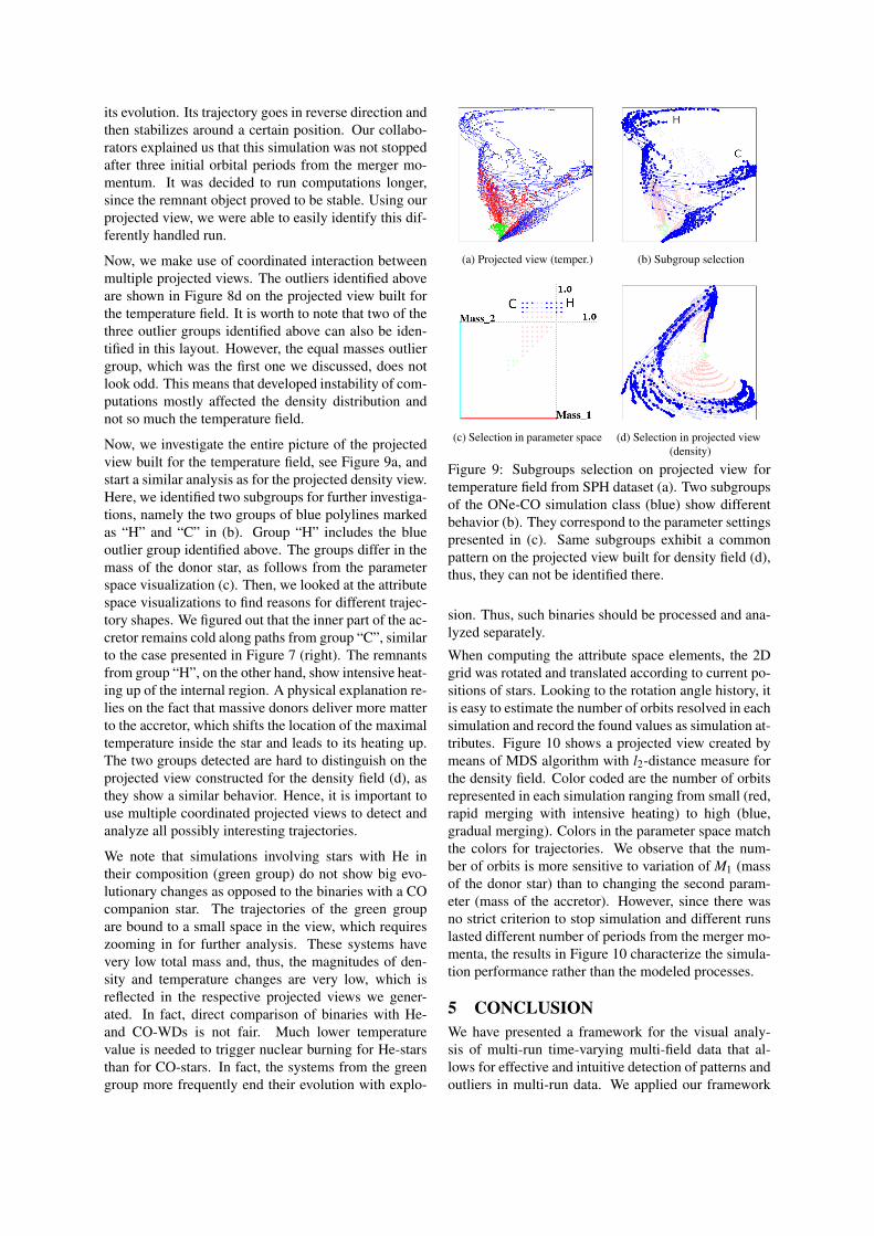
Now, we investigate the entire picture of the projectedview built for the temperature field, see Figure 9a, andstart a similar analysis as for the projected density view.Here, we identified two subgroups for further investiga-tions, namely the two groups of blue polylines markedas “H” and “C” in (b). Group “H” includes the blueoutlier group identified above. The groups differ in themass of the donor star, as follows from the parameterspace visualization (c). Then, we looked at the attributespace visualizations to find reasons for different trajec-tory shapes. We figured out that the inner part of the ac-cretor remains cold along paths from group “C”, similarto the case presented in Figure 7 (right). The remnantsfrom group “H”, on the other hand, show intensive heat-ing up of the internal region. A physical explanation re-lies on the fact that massive donors deliver more matterto the accretor, which shifts the location of the maximaltemperature inside the star and leads to its heating up.The two groups detected are hard to distinguish on theprojected view constructed for the density field (d), asthey show a similar behavior. Hence, it is important touse multiple coordinated projected views to detect andanalyze all possibly interesting trajectories.

We note that simulations involving stars with He intheir composition (green group) do not show big evo-lutionary changes as opposed to the binaries with a COcompanion star. The trajectories of the green groupare bound to a small space in the view, which requireszooming in for further analysis. These systems havevery low total mass and, thus, the magnitudes of den-sity and temperature changes are very low, which isreflected in the respective projected views we gener-ated. In fact, direct comparison of binaries with He-and CO-WDs is not fair. Much lower temperaturevalue is needed to trigger nuclear burning for He-starsthan for CO-stars. In fact, the systems from the greengroup more frequently end their evolution with explo-

(a) Projected view (temper.) (b) Subgroup selection

(c) Selection in parameter space (d) Selection in projected view(density)

Figure 9: Subgroups selection on projected view fortemperature field from SPH dataset (a). Two subgroupsof the ONe-CO simulation class (blue) show differentbehavior (b). They correspond to the parameter settingspresented in (c). Same subgroups exhibit a commonpattern on the projected view built for density field (d),thus, they can not be identified there.

sion. Thus, such binaries should be processed and ana-lyzed separately.

When computing the attribute space elements, the 2Dgrid was rotated and translated according to current po-sitions of stars. Looking to the rotation angle history, itis easy to estimate the number of orbits resolved in eachsimulation and record the found values as simulation at-tributes. Figure 10 shows a projected view created bymeans of MDS algorithm with l2-distance measure forthe density field. Color coded are the number of orbitsrepresented in each simulation ranging from small (red,rapid merging with intensive heating) to high (blue,gradual merging). Colors in the parameter space matchthe colors for trajectories. We observe that the num-ber of orbits is more sensitive to variation of M1 (massof the donor star) than to changing the second param-eter (mass of the accretor). However, since there wasno strict criterion to stop simulation and different runslasted different number of periods from the merger mo-menta, the results in Figure 10 characterize the simula-tion performance rather than the modeled processes.

5 CONCLUSIONWe have presented a framework for the visual analy-sis of multi-run time-varying multi-field data that al-lows for effective and intuitive detection of patterns andoutliers in multi-run data. We applied our framework

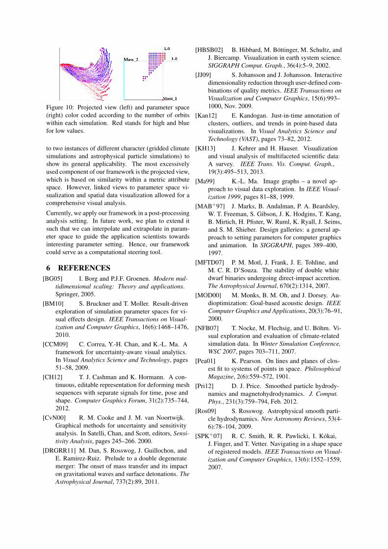
Figure 10: Projected view (left) and parameter space(right) color coded according to the number of orbitswithin each simulation. Red stands for high and bluefor low values.

to two instances of different character (gridded climatesimulations and astrophysical particle simulations) toshow its general applicability. The most excessivelyused component of our framework is the projected view,which is based on similarity within a metric attributespace. However, linked views to parameter space vi-sualization and spatial data visualization allowed for acomprehensive visual analysis.

Currently, we apply our framework in a post-processinganalysis setting. In future work, we plan to extend itsuch that we can interpolate and extrapolate in param-eter space to guide the application scientists towardsinteresting parameter setting. Hence, our frameworkcould serve as a computational steering tool.

6 REFERENCES[BG05] I. Borg and P.J.F. Groenen. Modern mul-

tidimensional scaling: Theory and applications.Springer, 2005.

[BM10] S. Bruckner and T. Moller. Result-drivenexploration of simulation parameter spaces for vi-sual effects design. IEEE Transactions on Visual-ization and Computer Graphics, 16(6):1468–1476,2010.

[CCM09] C. Correa, Y.-H. Chan, and K.-L. Ma. Aframework for uncertainty-aware visual analytics.In Visual Analytics Science and Technology, pages51–58, 2009.

[CH12] T. J. Cashman and K. Hormann. A con-tinuous, editable representation for deforming meshsequences with separate signals for time, pose andshape. Computer Graphics Forum, 31(2):735–744,2012.

[CvN00] R. M. Cooke and J. M. van Noortwijk.Graphical methods for uncertainty and sensitivityanalysis. In Satelli, Chan, and Scott, editors, Sensi-tivity Analysis, pages 245–266. 2000.

[DRGRR11] M. Dan, S. Rosswog, J. Guillochon, andE. Ramirez-Ruiz. Prelude to a double degeneratemerger: The onset of mass transfer and its impacton gravitational waves and surface detonations. TheAstrophysical Journal, 737(2):89, 2011.

[HBSB02] B. Hibbard, M. Böttinger, M. Schultz, andJ. Biercamp. Visualization in earth system science.SIGGRAPH Comput. Graph., 36(4):5–9, 2002.

[JJ09] S. Johansson and J. Johansson. Interactivedimensionality reduction through user-defined com-binations of quality metrics. IEEE Transactions onVisualization and Computer Graphics, 15(6):993–1000, Nov. 2009.

[Kan12] E. Kandogan. Just-in-time annotation ofclusters, outliers, and trends in point-based datavisualizations. In Visual Analytics Science andTechnology (VAST), pages 73–82, 2012.

[KH13] J. Kehrer and H. Hauser. Visualizationand visual analysis of multifaceted scientific data:A survey. IEEE Trans. Vis. Comput. Graph.,19(3):495–513, 2013.

[Ma99] K.-L. Ma. Image graphs – a novel ap-proach to visual data exploration. In IEEE Visual-ization 1999, pages 81–88, 1999.

[MAB+97] J. Marks, B. Andalman, P. A. Beardsley,W. T. Freeman, S. Gibson, J. K. Hodgins, T. Kang,B. Mirtich, H. Pfister, W. Ruml, K. Ryall, J. Seims,and S. M. Shieber. Design galleries: a general ap-proach to setting parameters for computer graphicsand animation. In SIGGRAPH, pages 389–400,1997.

[MFTD07] P. M. Motl, J. Frank, J. E. Tohline, andM. C. R. D’Souza. The stability of double whitedwarf binaries undergoing direct-impact accretion.The Astrophysical Journal, 670(2):1314, 2007.

[MOD00] M. Monks, B. M. Oh, and J. Dorsey. Au-dioptimization: Goal-based acoustic design. IEEEComputer Graphics and Applications, 20(3):76–91,2000.

[NFB07] T. Nocke, M. Flechsig, and U. Böhm. Vi-sual exploration and evaluation of climate-relatedsimulation data. In Winter Simulation Conference,WSC 2007, pages 703–711, 2007.

[Pea01] K. Pearson. On lines and planes of clos-est fit to systems of points in space. PhilosophicalMagazine, 2(6):559–572, 1901.

[Pri12] D. J. Price. Smoothed particle hydrody-namics and magnetohydrodynamics. J. Comput.Phys., 231(3):759–794, Feb. 2012.

[Ros09] S. Rosswog. Astrophysical smooth parti-cle hydrodynamics. New Astronomy Reviews, 53(4-6):78–104, 2009.

[SPK+07] R. C. Smith, R. R. Pawlicki, I. Kókai,J. Finger, and T. Vetter. Navigating in a shape spaceof registered models. IEEE Transactions on Visual-ization and Computer Graphics, 13(6):1552–1559,2007.