User Guide

Vision SoftwareMX280001A

Anritsu Company490 Jarvis DriveMorgan Hill, CA 95037-2809USAhttp://www.anritsu.com

Part Number: 10580-00418Revision: C

Published: December 2016Copyright 2016 Anritsu Company

Front-2 PN: 10580-00418 Rev. C MX280001A UG

TRADEMARK ACKNOWLEDGMENTSWindows, Windows XP, Microsoft Paint, Microsoft Word, Microsoft Excel, are all registered trademarks of Microsoft Corporation.GeckoFX and xulRunner are distributed under the Mozilla Public License V2.0.EasyGIS is distributed under the Lesser General Public License (LGPL).DotNetZip Libarry is distributed under the Microsoft Public License (Ms-PL).BetterListView ExpressgTrackBar is distributed under the Code Project Open License (CPOL) 1.02.WebSocket4Net is distributed under the Apache License 2.0 (Apache).https://developer.mozilla.org/en-US/docs/Mozilla/Gecko by Mozilla Contributors is licensed under CC-BY-SA 2.5https://developer.mozilla.org/en/XULRunner by Mozilla Contributors is licensed under CC-BY-SA 2.5OpenStreetMap® is open data, licensed under the Open Data Commons Open Database License (ODbL) by the OpenStreetMap Foundation (OSMF).

NOTICEAnritsu Company has prepared this manual for use by Anritsu Company personnel and customers as a guide for the proper installation, operation and maintenance of Anritsu Company equipment and computer programs. The drawings, specifications, and information contained herein are the property of Anritsu Company, and any unauthorized use or disclosure of these drawings, specifications, and information is prohibited; they shall not be reproduced, copied, or used in whole or in part as the basis for manufacture or sale of the equipment or software programs without the prior written consent of Anritsu Company.

UPDATESUpdates, if any, can be downloaded from the Documents area of the Anritsu Website at:http://www.anritsu.com

For the latest service and sales contact information in your area, please visit:http://www.anritsu.com/contact-us

MX280001A UG PN: 10580-00418 Rev. C Contents-1

Table of Contents

Chapter 1—Vision Trace Monitor

1-1 Introduction. . . . . . . . . . . . . . . . . . . . . . . . . . . . . . . . . . . . . . . . . . . . . . . . . . . . . . . . . . . . . . . . 1-1

1-2 System Requirements . . . . . . . . . . . . . . . . . . . . . . . . . . . . . . . . . . . . . . . . . . . . . . . . . . . . . . . 1-2

1-3 Tool Bar . . . . . . . . . . . . . . . . . . . . . . . . . . . . . . . . . . . . . . . . . . . . . . . . . . . . . . . . . . . . . . . . . . 1-2

1-4 Base Station (Spectrum Monitor) and Channel Directory. . . . . . . . . . . . . . . . . . . . . . . . . . . . . 1-5

1-5 Current Trace Panel . . . . . . . . . . . . . . . . . . . . . . . . . . . . . . . . . . . . . . . . . . . . . . . . . . . . . . . . . 1-8

1-6 Spectrogram . . . . . . . . . . . . . . . . . . . . . . . . . . . . . . . . . . . . . . . . . . . . . . . . . . . . . . . . . . . . . . . 1-9

1-7 Trace Matrix . . . . . . . . . . . . . . . . . . . . . . . . . . . . . . . . . . . . . . . . . . . . . . . . . . . . . . . . . . . . . . 1-10

1-8 Status Panel . . . . . . . . . . . . . . . . . . . . . . . . . . . . . . . . . . . . . . . . . . . . . . . . . . . . . . . . . . . . . . 1-11

Measurement Configuration . . . . . . . . . . . . . . . . . . . . . . . . . . . . . . . . . . . . . . . . . . . . . . . 1-11

Status . . . . . . . . . . . . . . . . . . . . . . . . . . . . . . . . . . . . . . . . . . . . . . . . . . . . . . . . . . . . . . . . 1-11

Mask Setup . . . . . . . . . . . . . . . . . . . . . . . . . . . . . . . . . . . . . . . . . . . . . . . . . . . . . . . . . . . . 1-12

Trace Mode . . . . . . . . . . . . . . . . . . . . . . . . . . . . . . . . . . . . . . . . . . . . . . . . . . . . . . . . . . . . 1-12

1-9 File Viewer . . . . . . . . . . . . . . . . . . . . . . . . . . . . . . . . . . . . . . . . . . . . . . . . . . . . . . . . . . . . . . . 1-13

File Navigation. . . . . . . . . . . . . . . . . . . . . . . . . . . . . . . . . . . . . . . . . . . . . . . . . . . . . . . . . . 1-13

1-10 Location Finder (Option 401) . . . . . . . . . . . . . . . . . . . . . . . . . . . . . . . . . . . . . . . . . . . . . . . . . 1-16

1-11 Time Difference of Arrival (TDOA) . . . . . . . . . . . . . . . . . . . . . . . . . . . . . . . . . . . . . . . . . . . . . 1-19

1-12 Probe Map . . . . . . . . . . . . . . . . . . . . . . . . . . . . . . . . . . . . . . . . . . . . . . . . . . . . . . . . . . . . . . . 1-27

1-13 Occupancy Report Generator. . . . . . . . . . . . . . . . . . . . . . . . . . . . . . . . . . . . . . . . . . . . . . . . . 1-28

Introduction . . . . . . . . . . . . . . . . . . . . . . . . . . . . . . . . . . . . . . . . . . . . . . . . . . . . . . . . . . . . 1-28

Trace Limitations . . . . . . . . . . . . . . . . . . . . . . . . . . . . . . . . . . . . . . . . . . . . . . . . . . . . . . . . 1-28

Report Generator. . . . . . . . . . . . . . . . . . . . . . . . . . . . . . . . . . . . . . . . . . . . . . . . . . . . . . . . 1-29

Generating the Report . . . . . . . . . . . . . . . . . . . . . . . . . . . . . . . . . . . . . . . . . . . . . . . . . . . . 1-30

Owner Lists . . . . . . . . . . . . . . . . . . . . . . . . . . . . . . . . . . . . . . . . . . . . . . . . . . . . . . . . . . . . 1-32

1-14 Copy & Paste Functions . . . . . . . . . . . . . . . . . . . . . . . . . . . . . . . . . . . . . . . . . . . . . . . . . . . . . 1-33

1-15 Limit Line Editor . . . . . . . . . . . . . . . . . . . . . . . . . . . . . . . . . . . . . . . . . . . . . . . . . . . . . . . . . . . 1-35

1-16 Status Bar . . . . . . . . . . . . . . . . . . . . . . . . . . . . . . . . . . . . . . . . . . . . . . . . . . . . . . . . . . . . . . . . 1-39

Chapter 2—High-Speed Port Scanner (Option 407)

2-1 Introduction. . . . . . . . . . . . . . . . . . . . . . . . . . . . . . . . . . . . . . . . . . . . . . . . . . . . . . . . . . . . . . . . 2-1

Installation of Vision Remote Monitoring Software Suite. . . . . . . . . . . . . . . . . . . . . . . . . . . 2-1

2-2 Running High-Speed Port Scanner . . . . . . . . . . . . . . . . . . . . . . . . . . . . . . . . . . . . . . . . . . . . . 2-1

2-3 Graphical User Interface. . . . . . . . . . . . . . . . . . . . . . . . . . . . . . . . . . . . . . . . . . . . . . . . . . . . . . 2-2

Contents-2 PN: 10580-00418 Rev. C MX280001A UG

Table of Contents (Continued)

2-4 Scan and Display Setup . . . . . . . . . . . . . . . . . . . . . . . . . . . . . . . . . . . . . . . . . . . . . . . . . . . . . . 2-4

2-5 Creating a High-Speed Port Scanner List. . . . . . . . . . . . . . . . . . . . . . . . . . . . . . . . . . . . . . . . . 2-6

2-6 Monitoring Channels . . . . . . . . . . . . . . . . . . . . . . . . . . . . . . . . . . . . . . . . . . . . . . . . . . . . . . . . . 2-7

2-7 Editing Sweep Parameters . . . . . . . . . . . . . . . . . . . . . . . . . . . . . . . . . . . . . . . . . . . . . . . . . . . . 2-7

2-8 Adding Limit Lines. . . . . . . . . . . . . . . . . . . . . . . . . . . . . . . . . . . . . . . . . . . . . . . . . . . . . . . . . . . 2-8

2-9 Saving and Loading Configuration Files . . . . . . . . . . . . . . . . . . . . . . . . . . . . . . . . . . . . . . . . . . 2-9

2-10 Viewing the Log File . . . . . . . . . . . . . . . . . . . . . . . . . . . . . . . . . . . . . . . . . . . . . . . . . . . . . . . . . 2-9

Chapter 3—Vision Acquire

3-1 Trace Setup . . . . . . . . . . . . . . . . . . . . . . . . . . . . . . . . . . . . . . . . . . . . . . . . . . . . . . . . . . . . . . . 3-2

Sweep Probes . . . . . . . . . . . . . . . . . . . . . . . . . . . . . . . . . . . . . . . . . . . . . . . . . . . . . . . . . . . 3-2

Max number of Threads. . . . . . . . . . . . . . . . . . . . . . . . . . . . . . . . . . . . . . . . . . . . . . . . . . . . 3-2

Logical Processors . . . . . . . . . . . . . . . . . . . . . . . . . . . . . . . . . . . . . . . . . . . . . . . . . . . . . . . 3-2

3-2 Database Setup . . . . . . . . . . . . . . . . . . . . . . . . . . . . . . . . . . . . . . . . . . . . . . . . . . . . . . . . . . . . 3-3

Automatically remove old traces . . . . . . . . . . . . . . . . . . . . . . . . . . . . . . . . . . . . . . . . . . . . . 3-3

Automatically archive trace tables . . . . . . . . . . . . . . . . . . . . . . . . . . . . . . . . . . . . . . . . . . . . 3-3

Sweep Once . . . . . . . . . . . . . . . . . . . . . . . . . . . . . . . . . . . . . . . . . . . . . . . . . . . . . . . . . . . . 3-3

Trim . . . . . . . . . . . . . . . . . . . . . . . . . . . . . . . . . . . . . . . . . . . . . . . . . . . . . . . . . . . . . . . . . . . 3-3

Compress . . . . . . . . . . . . . . . . . . . . . . . . . . . . . . . . . . . . . . . . . . . . . . . . . . . . . . . . . . . . . . 3-3

Archive. . . . . . . . . . . . . . . . . . . . . . . . . . . . . . . . . . . . . . . . . . . . . . . . . . . . . . . . . . . . . . . . . 3-3

View Log . . . . . . . . . . . . . . . . . . . . . . . . . . . . . . . . . . . . . . . . . . . . . . . . . . . . . . . . . . . . . . . 3-3

Database Path . . . . . . . . . . . . . . . . . . . . . . . . . . . . . . . . . . . . . . . . . . . . . . . . . . . . . . . . . . . 3-3

Advanced Database Scheduler . . . . . . . . . . . . . . . . . . . . . . . . . . . . . . . . . . . . . . . . . . . . . . 3-4

3-3 Notifications . . . . . . . . . . . . . . . . . . . . . . . . . . . . . . . . . . . . . . . . . . . . . . . . . . . . . . . . . . . . . . . 3-5

Send status emails . . . . . . . . . . . . . . . . . . . . . . . . . . . . . . . . . . . . . . . . . . . . . . . . . . . . . . . 3-5

Toolbar. . . . . . . . . . . . . . . . . . . . . . . . . . . . . . . . . . . . . . . . . . . . . . . . . . . . . . . . . . . . . . . . . 3-6

Version. . . . . . . . . . . . . . . . . . . . . . . . . . . . . . . . . . . . . . . . . . . . . . . . . . . . . . . . . . . . . . . . . 3-6

Progress Bar . . . . . . . . . . . . . . . . . . . . . . . . . . . . . . . . . . . . . . . . . . . . . . . . . . . . . . . . . . . . 3-6

Chapter 4—Vision Create Database

4-1 Base Station Database Creator Overview . . . . . . . . . . . . . . . . . . . . . . . . . . . . . . . . . . . . . . . . 4-1

Tool Bar . . . . . . . . . . . . . . . . . . . . . . . . . . . . . . . . . . . . . . . . . . . . . . . . . . . . . . . . . . . . . . . . 4-2

Probe Installation Details List . . . . . . . . . . . . . . . . . . . . . . . . . . . . . . . . . . . . . . . . . . . . . . . 4-3

Channel Definitions . . . . . . . . . . . . . . . . . . . . . . . . . . . . . . . . . . . . . . . . . . . . . . . . . . . . . . . 4-3

Mask Definitions . . . . . . . . . . . . . . . . . . . . . . . . . . . . . . . . . . . . . . . . . . . . . . . . . . . . . . . . . 4-3

Response Data Window . . . . . . . . . . . . . . . . . . . . . . . . . . . . . . . . . . . . . . . . . . . . . . . . . . . 4-3

4-2 How to. . . . . . . . . . . . . . . . . . . . . . . . . . . . . . . . . . . . . . . . . . . . . . . . . . . . . . . . . . . . . . . . . . . . 4-3

Set the Path for a Database File . . . . . . . . . . . . . . . . . . . . . . . . . . . . . . . . . . . . . . . . . . . . . 4-3

Update a Base Station Definition File . . . . . . . . . . . . . . . . . . . . . . . . . . . . . . . . . . . . . . . . . 4-3

Create a Database File Using a Base Station Definition File . . . . . . . . . . . . . . . . . . . . . . . 4-4

Create a Definition File (.def) or Database File (.mdb) Using a Database File . . . . . . . . . . 4-4

Create a Definition File (.def) or Database File (.mdb) Using a Base Station List File . . . . 4-4

Create a Database Manually . . . . . . . . . . . . . . . . . . . . . . . . . . . . . . . . . . . . . . . . . . . . . . . . 4-5

Set the Sweep Rate. . . . . . . . . . . . . . . . . . . . . . . . . . . . . . . . . . . . . . . . . . . . . . . . . . . . . . . 4-5

Import a Mask . . . . . . . . . . . . . . . . . . . . . . . . . . . . . . . . . . . . . . . . . . . . . . . . . . . . . . . . . . . 4-5

Database Utility . . . . . . . . . . . . . . . . . . . . . . . . . . . . . . . . . . . . . . . . . . . . . . . . . . . . . . . . . . 4-6

MX280001A UG PN: 10580-00418 Rev. C Contents-3

Chapter 5—Map Creation

Chapter 6—IQ Converter

6-1 Introduction. . . . . . . . . . . . . . . . . . . . . . . . . . . . . . . . . . . . . . . . . . . . . . . . . . . . . . . . . . . . . . . . 6-1

Load the IQ Capture File . . . . . . . . . . . . . . . . . . . . . . . . . . . . . . . . . . . . . . . . . . . . . . . . . . . 6-1

6-2 Data File Set Up . . . . . . . . . . . . . . . . . . . . . . . . . . . . . . . . . . . . . . . . . . . . . . . . . . . . . . . . . . . . 6-2

Set the Input File Type . . . . . . . . . . . . . . . . . . . . . . . . . . . . . . . . . . . . . . . . . . . . . . . . . . . . 6-2

Set the Input File Description . . . . . . . . . . . . . . . . . . . . . . . . . . . . . . . . . . . . . . . . . . . . . . . 6-2

Set the Output File Type . . . . . . . . . . . . . . . . . . . . . . . . . . . . . . . . . . . . . . . . . . . . . . . . . . . 6-3

Set the Output File Description . . . . . . . . . . . . . . . . . . . . . . . . . . . . . . . . . . . . . . . . . . . . . . 6-3

6-3 Converting the File . . . . . . . . . . . . . . . . . . . . . . . . . . . . . . . . . . . . . . . . . . . . . . . . . . . . . . . . . . 6-4

6-4 Resampling. . . . . . . . . . . . . . . . . . . . . . . . . . . . . . . . . . . . . . . . . . . . . . . . . . . . . . . . . . . . . . . . 6-5

6-5 IQ Capture . . . . . . . . . . . . . . . . . . . . . . . . . . . . . . . . . . . . . . . . . . . . . . . . . . . . . . . . . . . . . . . . 6-6

6-6 Play AM or FM Demodulated Signals. . . . . . . . . . . . . . . . . . . . . . . . . . . . . . . . . . . . . . . . . . . . 6-6

6-7 Converting MG3710A IQ Data File . . . . . . . . . . . . . . . . . . . . . . . . . . . . . . . . . . . . . . . . . . . . . . 6-6

Contents-4 PN: 10580-00418 Rev. C MX280001A UG

MX280001A UG PN: 10580-00418 Rev. C 1-1

Chapter 1 — Vision Trace Monitor

1-1 IntroductionVision Trace Monitor (0ption 400, works with Anritsu’s MS2710xA series remote spectrum monitors) is a program to analyze traces collected from spectrum monitors out in the field and placed in the Vision Monitoring database. Masks can be created to validate trace data. Spectrum monitor channel color coded icons indicate which channels have failed recently or have a high failure rate historically. Spectrum monitors not responding to sweep requests can be spotted because of the few traces stored in the database.

Starting the program will open the Vision Monitor user interface. On the left side of the interface will be the Spectrum Monitor and Channel Directory and the Status Panel. Another panel can be displayed by clicking on the three dots located at bottom right corner of the Spectrum Monitor and Channel Directory panel and selecting Trace History, Monitor Map, or Live Data Stream. The following panels will be displayed on the right hand side of the user interface: Trace Panel, Spectrogram, and Trace Matrix.

Figure 1-1. Vision Trace Monitor User Interface

1-2 System Requirements Vision Trace Monitor

1-2 PN: 10580-00418 Rev. C MX280001A UG

1-2 System Requirements • Microsoft Windows XP or Higher

• 4 GB of RAM

• 100 GB of hard-disk space

• Microsoft.Net Framework 4.0 or higher

1-3 Tool BarThe main options and application controls for Vision Monitor are found in the program toolbar. You can open a menu to configure software settings, pick a particular view mode, access advanced functionality, search for monitors by name or description and filter the monitor list based on various criteria options.

Figure 1-2. Vision Monitor Toolbar

Icon Description

Configuration: Opens a pull-down list:

Set Time Frame

Set Database Location

Recent Databases

Create a New Database

Show Location Estimate on Map

Preferred Web Browser

Use High Contrast Colors

Map Source

Panels Switch: Returns to the spectrum measurement, spectrogram and time matrix panels from either the live data stream window or monitor map window.

Show Probe Map: Displays a larger map for the current trace channel selected on the right side where the trace panel, spectrogram, and trace matrix were located.

Live Data Stream: Click on this button to live stream the selected current spectrum monitor display.

Vision Trace Monitor 1-3 Tool Bar

MX280001A UG PN: 10580-00418 Rev. C 1-3

Open Trace Viewer Window: Allows you to view multiple channels at one time either in the current trace mode or spectrograph mode. In the Spectrum Monitor and Channel Directory, hold down the Ctrl key on the keyboard and use the mouse to select multiple channels. Selected channels will be highlighted in dark blue.

High-Speed Port Scanner: Refer to Chapter 2, “High-Speed Port Scanner (Option 407)” for information about this application.

Remote File Viewer: Click to run the “File Viewer” application.

Load Selected Channels: Loads the selected channels into the Trace Viewer window to view simultaneously.

Open a saved window list: Opens the Open dialog to load a *.vwl file, Vision Windows List. Select the desired file to load. Save Window List saves the currently displayed trace window selections for future loading. Previously opened VWL files will list under this command.

“Location Finder (Option 401)”: Opens the Source Locater window to geo-locate the signal of interest.

Generate Pass/Fail Report: Creates a Vision Monitor Failure & Status Report that will be displayed in your Internet browser.

Generate Failure Report: Produces a failure and status report and displays it it the current default Web browser.

Export Failure Report: Produces the a failure and status report, exactly the the one produced by Generate Failure Report, but outputs the data into a .txt file with the name Vision Status + date stamp + time stamp.txt. The file is placed in the folder set using the Report Options function.

Occupancy Report Generator: See “Occupancy Report Generator”

Browse Report Archive: Opens the folder set in Report Options, allowing you to review or open files exported to that folder.

Report Options: Opens the Vision Reports Options dialog. Here you can set the Failure Report Options, Occupancy Report Options, select the folder for exported files, and the field delimiter for exported files. If Archive Reports is selected, enter a folder location or click the Select Browser and navigate to the desired folder to archive the reports. If Archive Reports is not selected, the report is a temporary file and will be lost when closed. You can add a header and footer to the report by clicking the respective Report Header and Report Footer check box. If selected, enter a folder location or click the Select Browser and navigate to the desired folder to archive the reports.

Copy & Paste: Press this list arrow to display the various copy and paste functions. Click on the desired Copy/Paste function.

Search for base station: Instead of scrolling through a long list of spectrum monitors, enter the name of the desired base station and click on the Binocular.

Icon Description

1-3 Tool Bar Vision Trace Monitor

1-4 PN: 10580-00418 Rev. C MX280001A UG

Filter: Allows you to view a specific category group of monitors on the current map. No Filter - Show All is the default view. The filter categories are:

No Filter Show All: All of the spectrum monitors in the Base Station list are displayed in the map.

Filter by Map: Only base stations viewed in the map will be displayed in the Base Station list. You must be in Probe Map view.

Failure by Last Sweep: Base stations with channels whose last trace failed will remain on the list and displayed in Map view.

Failure in Past Hour: Base stations with channels that had a trace fail within the last hour will remain on the list and displayed in Map view.

Failure in Past Day: Base stations with channels that had a trace fail within the day will remain on the list and displayed in Map view.

Help: Press to open Vision Help.

Icon Description

Vision Trace Monitor 1-4 Base Station (Spectrum Monitor) and Channel Directory

MX280001A UG PN: 10580-00418 Rev. C 1-5

1-4 Base Station (Spectrum Monitor) and Channel DirectoryThe list on the left contains the names of the spectrum monitors. Columns numbered one through twelve are the spectrum monitor channels.

Figure 1-3. Base Station (Spectrum Monitor) and Channel Directory

1-4 Base Station (Spectrum Monitor) and Channel Directory Vision Trace Monitor

1-6 PN: 10580-00418 Rev. C MX280001A UG

You can also configure a specific monitor through the use of its context menu. Highlight the desired spectrum monitor and click the right mouse button. The context menu below opens.

Icon Description

These bars represent channels and indicates the varying passing percentages of traces within the channel.

The light blue outline indicates the current channel selected. The last trace collected from the spectrum monitor will be displayed in the Trace Preview Panel, highlighted as a yellow line in the Spectrogram Pane, and outlined as a white square box in the Trace Matrix panel. In the Probe Map view, the spectrum monitor and channel will be indicated as a bouncing pin.

The bars outlined in red indicate the last trace collected for that channel failed.

Multiple channels that have been selected are outlined in dark blue. These channels are used with the Open Trace Viewer Window feature or with the Location Finder feature.

Figure 1-4. Base Station (Spectrum Monitor) Context Menu

Vision Trace Monitor 1-4 Base Station (Spectrum Monitor) and Channel Directory

MX280001A UG PN: 10580-00418 Rev. C 1-7

• Open Probe Web UI in Browser: Opens the Installed Web Browsers dialog to select either Google Chrome or IEXPLOR.EXE.

• Ping Selected Probe: Establishes communication with the monitor. The Vision Ping dialog opens displaying the reply information from the monitor.

• Rename Selected Probe: Opens the Edit Base Station dialog to change the label of the selected monitor. Enter a new name in the entry box.

• Retrieve & Update GPS Location: Does an immediate query to the monitor for updated GPS location.

• Update Probe Options: To update any changes in options, this button must be pressed. A dialog will pop up stating if the update was successful and which spectrum monitors were successfully updated.

• Edit Probe URL (Host name or IP): Opens the Edit Base Station URL dialog to change the URL of the selected remote spectrum monitor. Enter a new URL in the entry box.

• Edit Description: Opens the Edit Base Station Description dialog to change the description of the selected remote spectrum monitor. Enter a new description in the entry box.

• Edit Contact E-mail: Opens Edit Base Station Contact dialog to add or change the e-mail address to those monitoring this base station. Add or change the e-mail address in the entry box.

• Enter Probe Height: Opens the Probe Height dialog to add or to change the height location of the selected remote spectrum monitor. Enter the new height in the entry box. Units are in meters.

• Set Probe Web Port: Opens the HTTP port # dialog. Enter the HTTP port number for this remote spectrum monitor. If assistance is needed in obtaining this port number, contact the person setting up the network for remote spectrum monitoring.

• Add New Probe to Database: The Create New Base Station dialog opens to enter information for the new database. Fill in the entries and press OK. The new monitor is listed on the Base Station & Channel Directory.

• Delete Selected Probe from Database: Allows you to delete a base station from the directory.

• Enable Sweep on All Channels: Enables data collection for each channel on a monitor. This can be done one at a time by clicking on the 'Unlock sweep parameters' check box, then checking the check box for 'Automatically monitor this channel'. Enable Sweep on All Channels is a quick way to do all channels on a monitor at once, rather than the tedious process of enabling each separately.

• Disable Sweep on All Channels: Disables data collection for all channels on a monitor. This can be done one at a time by clicking on the 'Unlock sweep parameters' check box, then clearing the check box for 'Automatically monitor this channel'. Disable Sweep on All Channels is a quick way to do all channels on a monitor at once, rather than the tedious process of disabling each separately.

• Probe Groups: Monitors can be assigned into groups. Groups are used only to visually arrange the monitors so that associated monitors are together in the monitor list. By default, the monitors are listed in the order they are entered into the database. To place the monitors in groups, use the monitor context menu to add and assign groups. You also must toggle the Show Groups setting on to see the grouped monitor list. Individual groups can be collapsed or expanded to easier view just the monitors that are of interest at a particular time.

1-5 Current Trace Panel Vision Trace Monitor

1-8 PN: 10580-00418 Rev. C MX280001A UG

1-5 Current Trace PanelWhen a channel is selected, the last trace collected in the database is displayed. Use the Scroll bar at the bottom of the display to view all of the other traces for the selected channel and base station. Figure 1-5 Trace Panel is an example of a Trace Matrix block that contains only one trace. The bar above the trace display will display the monitor and channel, frequency and amplitude at the cursor location, and a selection box to display only failed traces. The power displayed is the power at that frequency not at the location of the cursor. If the Display Failed Traces Only box is checked only traces that failed the limit line mask are shown in the trace display, spectrogram, and trace-matrix. Markers can be set by placing the cursor at a desired location and clicking the left mouse button. An orange horizontal line will be drawn and the frequency and amplitude of that location will display under the x-axis. A second marker, red delta marker, can be displayed by clicking at any other location on the trace display. Frequency and power delta information will display right of the main marker information under the x-axis. See also Figure 1-8, “Trace Matrix with One Trace per Block”.

If you select a block in the Trace Matrix that contains more than one trace, all the traces for that block are drawn simultaneously in the trace panel. See Figure 1-9, “Trace Matrix with Multiple Traces per Block”. Four buttons will appear in the upper right corner of the display. These buttons allow you to select between seeing all selected traces as overlays, apply for Min Hold, Max Hold, or Averaging modes to the traces.

Figure 1-5. Trace Panel

Figure 1-6. Trace Panel with Multiple Traces in Data Block

Vision Trace Monitor 1-6 Spectrogram

MX280001A UG PN: 10580-00418 Rev. C 1-9

1-6 SpectrogramDisplays all of the traces collected from the 12 channels of the selected base station. The trace displayed in the Current Trace Panel is indicated by the short white line at the left edge of the display panel. If the number of traces exceed the display, a scroll bar will appear on the right that will allow you to view all of the traces. A power range color indicator resides left of the spectrogram which defines the trace colors in the spectrogram. A day, date, and time stamp will display under the power range color indicator for a trace that the cursor points to in the spectrogram.

Figure 1-7. Spectrogram

1-7 Trace Matrix Vision Trace Monitor

1-10 PN: 10580-00418 Rev. C MX280001A UG

1-7 Trace MatrixUseful to observe interference signal patterns that are occurring based on time and day. In Figure 1-8, “Trace Matrix with One Trace per Block”, each block is 5 seconds and a row a tenth of an hour. Depending on the length of time measurements are taken, the amount of traces can fill the matrix display. If that occurs, use the vertical scroll bar of the display to view the other blocks of measurements.

The Color Bars button allow you to change the color scheme of the of the data blocks in the matrix from green, red, and yellow to blue, yellow, and green.

Depending on how you set up data collection, multiple traces can be collected during one data block. In that case green means all traces in the block pass. Red means all traces in the block fail. Yellow means that some pass and some fail. For example, data collection is set to 10 seconds and the time frame in Vision Monitor is set to 6 hours making a data block 20 seconds long. This results in acquiring two traces for each data block and the color coding shown in Figure 1-9, “Trace Matrix with Multiple Traces per Block”. Click on a colored square to view the associated trace in the Trace Panel or Spectrogram.

Figure 1-8. Trace Matrix with One Trace per Block

Figure 1-9. Trace Matrix with Multiple Traces per Block

Vision Trace Monitor 1-8 Status Panel

MX280001A UG PN: 10580-00418 Rev. C 1-11

1-8 Status PanelThe Status Panel is a combination of setup and status.

Unlock sweep parameters: Allows for information in this panel to be changed.

Measurement Configuration

Measurement Configuration contains the setup parameters of the spectrum monitor in the field. If desired, they can be changed in their respective edit boxes.

• Start Frequency

• Stop Frequency

• RBW

• VBW

• Reference Level

• Ref. Level Offset

• Trace Points

• Sweep Time

• Preamp

• FFT

Status

• Pass Rate: Displays the total number of traces in the channels, the number of traces that passed, and the pass percentage.

• Last Sweep: Date and time of the last sweep.

• Last Fail: Date and time of the last trace that failed.

• Sector: The direction of the antennae in relation to north.

• Frequency: The center frequency of the transmission band.

Figure 1-10. Status Panel

1-8 Status Panel Vision Trace Monitor

1-12 PN: 10580-00418 Rev. C MX280001A UG

Mask Setup

1. Check the Unlock sweep parameters box. This allows parameter changes and editing.

2. To create a new mask, press Mask Editor to open the Limit Line Editor. Go to Step 5.

3. For existing masks, press the down arrow for Mask to display the list of masks.

4. Highlight and click on the desired mask.

5. Use the tools in the toolbar to edit or create a mask.

Next to the Mask Editor button is the Apply Mask To button. When pressed, it opens the Apply Mask To dialog. You can apply the selected mask in the limit line list to historical trace data in the database. You can choose to apply the mask to the selected channel, the current base station, all channels in the column or all channels in the table. Masks can also be applied to channels within a group or base stations within a groups. These groups were previously made using the Probe Groups function int the Base Station Context Menu or when creating a database. When a mask is applied to trace history, the status of previously collected traces is updated as are pass/fail statistics for the channels affected. Changing the mask in the list affects future traces acquired, but not the status of traces already stored in the database. To summarize:

• To change the mask only for future traces, change the mask without clicking on Apply.

• To change the mask for both past traces and for future traces, click on Apply.

Refer to Section 1-15 “Limit Line Editor” for more mask editing information.

Trace Mode

Select the desired Trace Mode Setting.

• Normal Trace: Displays data for the current trace sweep.

• Rolling Min: Minimum value at each frequency point over the last trace sweeps.

• Rolling Averaging: Average value at each frequency point over the last trace sweeps.

• Rolling Max: Maximum value at each frequency point over the last trace sweeps.

• Trace Count: The number of traces to be used for rolling minimum, maximum, and average.

Vision Trace Monitor 1-9 File Viewer

MX280001A UG PN: 10580-00418 Rev. C 1-13

1-9 File ViewerUse File Viewer to open and view RSM and CPM files. RSM files can be retrieved and viewed from a Remote Spectrum Monitor or as a saved file. View CPM files from a saved file.

File Navigation

Click the Location Type drop-down list. Select the desired location for the file type to be viewed.

• Remote Spectrum Monitor: Click Remote Spectrum Monitor to obtain an RSM file from a Remote Spectrum Monitoring instrument.

• Local Measurement Folder: View RSM files in a folder on a local drive.

• CPM Measurement File: View CPM files in a folder on a local drive.

Remote Spectrum Monitor

1. Type a Host Name or URL for the instrument whose measurements you want to view.

2. Press Enter. A list of RSM and STP files are listed.

3. Double click on the desired RSM file to view immediately

4. Click the check box to select specific RSM file or the Select All check box to download files to a local drive.

5. Press Download. The Browse For Folder opens. Navigate to the desired foleder to save the selected files.

Figure 1-11. Remote Spectrum Monitor Panel

1-9 File Viewer Vision Trace Monitor

1-14 PN: 10580-00418 Rev. C MX280001A UG

Local Measurement Folder

1. Press Path to navigate to the folder which contains RSM files or enter a path and folder where the RSM files reside on the local drive. Below the Trace List, data related to the trace is displayed.

2. Click on the desired RSM trace to view in the display.

3. Add and remove Markers. Add a Marker and/or delta Marker by placing the mouse cursor on the desired frequency and pressing the left mouse button. Remove the Markers by unchecking the check boxes at the left bottom corner of the display.

At the bottom right corner of the display the values of the Occupied Bandwidth (OBW) and Channel Power is displayed.

Figure 1-12. Local Measurement Folder Panel

Vision Trace Monitor 1-9 File Viewer

MX280001A UG PN: 10580-00418 Rev. C 1-15

CPM Measurement File

1. Press Filename to navigate to the folder which contains the CPM files or enter a path and folder where the CPM files reside on the local drive.

2. Press Enter. A list of channels will display.

3. Click the desired channel. Two windows will be displayed - trace and spectrogram.

At the top right corner of the trace display are buttons for various view modes:

• Single Trace: Default view showing only one trace, the last measurement trace taken.

• All Traces: Shows all of the traces taken during a set period for the selected channel

• Min Hold Trace: Shows the cumulative minimum value of each display point

• over many trace sweeps.

• Max Hold Trace: Shows the cumulative minimum value of each display point over many trace sweeps.

• Average Trace: Shows an exponential average of a number of traces, determined by the # of Averages key.

Figure 1-13. CPM Measurement File Panel

1-10 Location Finder (Option 401) Vision Trace Monitor

1-16 PN: 10580-00418 Rev. C MX280001A UG

1-10 Location Finder (Option 401)Review the data from the Base Station and Channel Directory. Hold down Ctrl on the keyboard and click up to three channels in the area where an interfering signal is suspect. Or, just select the problem channel and let Vision Trace Monitor select the two closest monitors automatically. Up to 10 nearby probes are selected and accessible from the Locator window. Then press the Location Finder button to open the Source Locater window.

If you have selected three monitors and have tried to open the Locater window but a message pops up informing you that they could not be found, it is possible the options looked for are not installed on the monitors. The monitors may have the options installed but the database needs to be updated. The monitor context menu has an selection to update the monitor options to the database. See also Figure 1-37, “Status Bar”.

The trace panels on the right side of the window are the signals from the base stations selected in descending order. A mini tool bar is above the top trace panel that includes the buttons:

• Sync: Use Sync to toggle time synchronization between the three monitors used in the location algorithm. Each trace graph has a horizontal scroll bar that allows the user to scroll through the trace history and look for a particular trace that exhibits the interference most strongly.

• Live: Initially when the Source Locator opens, the last sweep taken is displayed in the trace panels for each of the selected monitors. Press Live to view the trace measurements in real-time.

• Sweep Config: Press this button to open a sweep configuration dialog. This allows you to adjust the sweep parameters for each of the monitors. This is useful for viewing live sweep data – it does not affect the sweep parameters stored in the database.

• 3 Probes/1 Probe/TDOA List: Select the desired monitor quantity for POA or TDOA interference signal hunting. To view signals at a single monitor, select 1 Probe from the Probe pull-down list above the top trace display. 1 Probe detection is only useful if the interferer can be seen in the sweep data on two more channels on the same monitor. Click 3 Probes in the pull-down list to triangulate the interferer position when the signal of interest can be seen on three near-by monitors. Click TDOA for locating an RF emitter using the Time Distance of Arrival geo-location algorithm.

Also at the top right corner of the three trace displays is a pull-down list. See Figure 1-16, “Source Locator Map”.Use this list to select another channel in triangulating an interferer signal. Typically this is used at cellular base station locations where multiple sectors are used. the bars on each icon indicate the direction for each antenna used in a sectored system. When the Source Locator window opens, a best guess determination for channels is made for the three monitors. You can select a different channel from the pull-down list. Select a channel that is closest in direction and frequency to the interferer signal.

Figure 1-14. Location Finder Button

Figure 1-15. Channels Selected for use with Location Finder

Vision Trace Monitor 1-10 Location Finder (Option 401)

MX280001A UG PN: 10580-00418 Rev. C 1-17

Another function for fine tuning the frequency when searching for the interferer is using the traces shown in the Location window on the right-hand column. Click in a trace display and a red marker line will show. Move the marker line by:

• placing the cursor on the desired frequency and clicking the left mouse button

• scrolling the mouse wheel till the red marker line is on the desired frequency

• pressing the left or right mouse buttons to the desired frequency.

• typing the desired frequency into the entry box.

The geo-location algorithm will be employed on the signal whose frequency is indicated by the vertical red line in all three traces.

Figure 1-16. Source Locator Map

1-10 Location Finder (Option 401) Vision Trace Monitor

1-18 PN: 10580-00418 Rev. C MX280001A UG

Once in the Source Locator Map, you can select another monitor that may provide better data for triangulating the interferer signal. Click on one of the active three monitors, numbered and colored red), or click on the side or bottom border of the desired trace panel. Click on a base station, symbolized by yellow square with a black star, to become the new active monitor. It becomes numbered and red. If you switch from 3 Probes to 1 Probe, this new active probe is used.

Icon Description

Spectrum monitors selected on the Base Station and Channel Directory to locate the interfering signal. The short lines that extend out from the square depict the direction of the antenna used. For a view of the interfering signal’s bearing used a single monitor, click the desired monitor represented by a number or star then select 1Probe from the Probe pull-down list above the top trace display.

Base Stations that are close by that can be used to locate the interfering signal. Click on this base station icon to make it one of the three base stations locating the interfering signal. At the same time, the last active number icon base station will turn into a star icon. The trace for the base station will change accordingly in the trace panel.

The approximate location of the interfering signal based on the information from the selected base stations.

Vision Trace Monitor 1-11 Time Difference of Arrival (TDOA)

MX280001A UG PN: 10580-00418 Rev. C 1-19

1-11 Time Difference of Arrival (TDOA)

Introduction

Vision Monitor includes two algorithm methods for locating RF emitter signals - Power of Arrival (POA) and Time Difference of Arrival (TDOA). Power of Arrival (POA) is the default location algorithm for locating interference signals and it places a bullseye icon on the map to indicate a location estimation. TDOA is a method for locating an RF emitter based on the differential time of arrival of the transmitted signal to 3 or more remote probes. TDOA may not always produce a single unique estimation, so the POA estimate can help in choosing the most likely location for the RF source.

Time Difference of Arrival (TDOA) is a very powerful technique to locate interference sources and other modulated broadcasters. However, it is not universally useful, and it does take considerable care and experience to use it effectively. Many sources of interference are CW or just noisy electronics. There is nothing about these type of signals that can be time-aligned and those emitters will not be locatable with TDOA.

To use TDOA to locate interference sources, the following considerations need to be made:

• The source must be modulated. TDOA looks for features in the RF spectrum as measured at 3 locations. Those features are time-aligned, and the difference in the time for the signals to reach each receiver is used to calculate the location. If the signal of interest does not have features that can be aligned in time, then TDOA will produce meaningless results. Typically that means the signal must be modulated.

• A clean IQ diagram produces much more accurate results. The better you can setup the spectrum monitor to capture IQ data, the more accurate the position estimate will be. This means more time may be needed to set up each remote monitor, adjusting the frequency, span, reference level and preamp settings to get the best possible IQ capture. Strong signals that are close by will be relatively better, but weaker signals, and especially distant signals take some care to get meaningful results.

• Distance matters. 3 remote monitors are used to do the TDOA triangulation of the RF source. Best results will be achieved if the source is contained inside a triangle made by connecting the remote monitor locations. TDOA works for sources outside this triangle, and may be used to locate a source that is many kilometers outside the triangle, but it is more accurate for sources that are close by.

The reason distance matters is due to the uncertainty in any measurement made. We are looking for the intersection of three lines. Where those lines intersect at nearly right angles, then any uncertainty in the line positions produces a similar uncertainty in the intersection. However, if the lines approach each other at very shallow angles, then the lines may be within the distance of uncertainty for several kilometers. Distant sources outside the triangle of the remote monitors will almost always produce lines that have very small incident angles, and that can greatly multiply the uncertainty in position.

TDOA requires additional set ups and IQ Capture. This chapter provides exercises for the following setup and monitoring activities:

• TDOA Settings & Control Setup

• IQ Capture Settings

• View IQ Capture Results

• Generating a TDOA Report

1-11 Time Difference of Arrival (TDOA) Vision Trace Monitor

1-20 PN: 10580-00418 Rev. C MX280001A UG

Settings & Control Setup

To use TDOA, confirm the remote monitors are installed with the TDOA option and need to be a part of the Vision database.

1. Select a channel of a probe of interest from the Probe List.

2. Press the Location Finder button in the main Vision Monitor toolbar.

3. The Vision Source Locater Window opens, the trace data loads and accompanying geo-location map opens.

4. Click on any of the trace graphs to set the frequency of the interference source.

5. Select TDOA from the Location Method drop down list.

Pro

Figure 1-17. Spectrum Monitor List and Location Finder Button

Figure 1-18. Trace Graph and Location Method Drop Down List

Vision Trace Monitor 1-11 Time Difference of Arrival (TDOA)

MX280001A UG PN: 10580-00418 Rev. C 1-21

IQ Capture Settings

Bit resolution - Allowed values are 8-bit, 10-bit, 16-bit and 24-bit. 16-bit is the recommended setting. Lower bit-resolution is faster to transmit, but provides less precise results.Higher bit resolution is slower to transmit but provides more precise results.

Spectrum Monitor Input Parameters (These parameters are used to set up the remote spectrum monitors. Set the parameters as desired.)

• Capture Bandwidth (BW)

• Capture Length

• Center Frequency

Start Data Collection: When pressed, Vision will repeatedly execute the TDOA measurement. New TDOA results are only averaged when the Correlation Ratio is higher than 30. After being pressed, the button will change to Stop Data Collection. Press it to end data collection.

The bottom line in the Correlation Results box shows the averaged distance in meters, and the number of averages used. The number of averages can be different for each set of probes because the correlation ratio may sometimes be too low for a particular probe pair.

Interpolate to increase resolution: When checked, each I/Q data set is resampled to a higher sampling rate. This gives greater spatial resolution. This slows down the correlation calculations. Narrow capture bandwidths use a lower sampling rate which limits the spatial resolution possible. Resampling can increase the spatial resolution, although manufactured data points are never as accurate as real data points. This only makes sense if the sampling rate is so low that the intrinsic sample rate does not fully capture features in the I/Q data.

Figure 1-19. TDOA Settings & Control Window

1-11 Time Difference of Arrival (TDOA) Vision Trace Monitor

1-22 PN: 10580-00418 Rev. C MX280001A UG

Remove dead-time...: When checked, two events occur:

• The program to waits until the power level on the first probe is within 10 dB of the reference level before the I/Q acquisition begins.

• After the I/Q data is acquired, it looks to see if there is dead time in the data set where the signal is missing. This dead-time is removed before th correlation is performed.

Automatically adjust capture length: When this is checked, the Capture Length input field is locked and cannot be user adjusted. Any adjustment to the Capture Bandwidth will automatically set the Capture Length to the optimal value.

The hardware adds a time stamp every 64k sample points. For narrow-bandwidth captures the sample rate is low, and if the capture length is too short there will not be enough data to include multiple time stamps. This leaves the actual sample rate unknown and the data is not usable.

You can clear this check box to be able to manually enter a desired capture length. This is useful if you want to capture a longer data stream. It is not useful to use a shorter capture length. When checking this box, the capture length will automatically adjust to the optimal value for the current capture bandwidth.

Automatically set reference levels: When this is checked, Vision will do a 20 sweep max-hold RF trace capture to determine the optimal reference level setting. It is important to use a reference level that is near the peak amplitude of the signal that is being sought. This maximizes the dynamic range and gives much better I/Q sample points. If the reference level is set too high, the I/Q plot will not fill in solid, but instead the points will appear in distinct rows and columns. This is equivalent to using a much lower bit resolution.

Average Distances: This check box is at the bottom row of the correlation results. Each time a TDOA I/Q capture is done, the distance result will be averaged with previous measurements. The resulting average values are shown along the line to the right of this check box. Checking the Average Distance (meters) check box causes the average values to be used when drawing the arcs on the map and locating the RF source. If the check box is clear, then the most recent measurement values will be used on the map, rather than the average values.

The values shown in the Averages look different. For example: -235 (12). The first number is the averaged value taken from the Correlation Offset (meters) field above. The number in parenthesis is the count of values used in the average. This can be a different number for each probe pair, depending on the Correlation Ratios from each measurement.

There is a X Clear Averages button below the Average Distances check box. This button will clear the averages. This should be done if you change which probes are being used, or if you change the frequency of the source you are looking for.

Mean capture time: This window displays the average time it takes to capture individual trace data.

Channel Delay Calibration: This button with the symbol of a clock is for experienced users only.

Once the above parameters have been set, IQ Capture may begin.

Press Start Data Collection. This process will take a few moments. Each remote probe is sent commands to configure the spectrum monitor as specified. Then IQ capture is initiated. It is essential for IQ captures to be synchronized in time, so each monitor will begin capturing data at the next GPS synchronization signal. The capture time is typically fairly short, several 10’s or 100’s of milliseconds. After IQ data has been captured on the remote monitors, it must be transferred over the network to the PC running Vision. This transfer can be slow, depending on the bandwidth available for communication with the remote monitors. The IQ data sets are very large, typically 10’s of megabytes. Press Stop Data Collection when you decide sufficient data has been collected.

Vision Trace Monitor 1-11 Time Difference of Arrival (TDOA)

MX280001A UG PN: 10580-00418 Rev. C 1-23

There are four progress bars below the IQ Capture Settings section of the dialog window. The first will show activity as the monitors are configured and the IQ data is actually captured. The other three progress bars indicate the progress, for each of the monitors, at transferring the data. The color bars will be completely filled once the capture is complete. The transfer is typically the longest part of this process. The progress bars are color coded to match the IQ charts.

At the completion and calculation of the IQ data, you can see the results in the Correlation Results section of the TDOA dialog window. In the diagram above, a yellow, green and blue line are also drawn on the map of the Locater Window. Each line represents a path that has the same distance differential from two of the monitors. The TDOA algorithm indicates that the source is located somewhere along that path. By using a set of three monitors, we get three distant paths. The intersection of all three paths marks the location of the RF source. A green square marker with a star is placed on the map at the intersection of the lines.

Figure 1-20. TDOA Settings & Control Window, Location Window, and Correlation Result

1-11 Time Difference of Arrival (TDOA) Vision Trace Monitor

1-24 PN: 10580-00418 Rev. C MX280001A UG

View IQ Capture Results

In the figure shown, there are two intersection points designated by the green squares with a star. One is inside the triangle, near monitor 1. Here the lines approach each other at large angles and an uncertainty of say 50 meters in each line position produces a similar uncertainty in the intersection point. However, in this case the true source was the one located in the upper left-hand of the image. In this case the lines actually are within 50 meters of each other for a distance of almost 500 meters.

• The TDOA Settings & Control window will show some results that help in judging how much confidence to have in a given set of data, and in the results produced. The last two lines of the results section contain the Correlation Ratio and IQ Similarity.

Figure 1-21. Remote Monitor Lines

Vision Trace Monitor 1-11 Time Difference of Arrival (TDOA)

MX280001A UG PN: 10580-00418 Rev. C 1-25

Correlation Ratio

The Correlation Ratio is a number that relates to how strongly the algorithm was able to find the correct time alignment offsets. The correlation peaks at the position where the two sets of IQ data are aligned in time. If this peak is very pronounced, then you can have confidence in the time alignment. If it is not so pronounced, then the data is suspect. Basically, the Correlation Ratio is the peak amplitude divided by the average value of the correlation function. A value less than 20 means you should not trust the results at all, while a value above 100 is usually a strong indication that the correlation is good.

Figure 1-22. Correlation Ratio

1-11 Time Difference of Arrival (TDOA) Vision Trace Monitor

1-26 PN: 10580-00418 Rev. C MX280001A UG

Generate a TDOA Report

After collecting TDOA data, press the Generate Report button to create a TDOA report within your browser.

Figure 1-23. TDOA Report

Vision Trace Monitor 1-12 Probe Map

MX280001A UG PN: 10580-00418 Rev. C 1-27

1-12 Probe MapClicking the Show Probe Map button, the right side panel will change to Probe Map view. The blue pins displayed represent the base stations in the Base Station and Channel Directory window. The highlighted base station in the Base Station and Channel Directory will be represented by a bouncing blue pin. The map can be viewed in street map, terrain, and satellite modes. Use the + and – buttons to zoom in and out of the map. Use the drag mode of the cursor to adjust the location view of the map. Drag the person icon to the location of the pin to get a ground level view of that location. Use the Filter on the Tool Bar to view base stations based on specific criteria.

If you do not have an Internet connection or if Google Maps is not allowed at your location, you can use an already developed map or create a map using OpenStreetMap for off-line viewing. For more information see Chapter 5, “Map Creation”.

Figure 1-24. Monitor Map

1-13 Occupancy Report Generator Vision Trace Monitor

1-28 PN: 10580-00418 Rev. C MX280001A UG

1-13 Occupancy Report Generator

Introduction

An occupancy report divides up a frequency range into sub-channels and shows the typical traffic at each sub-channel frequency. Occupancy reports are typically used to investigate the availability of bandwidth within a particular frequency space or to locate unexpected signals in the frequency space. Occupancy reports are generated from several hours, days, or weeks of continuous spectrum monitoring data. Unlike other reports in Vision, Occupancy Reports may span multiple databases.

The first step is to determine the frequency range of interest and then to collect trace data in that frequency space. The remote monitors can collect up to 4000 points per trace. You will need to set the number of points such that you have at least one point/sub-channel. If you have more than one point/sub-channel, the highest measured power in the sub-channel is used in the report. For instance, if you are interested in monitoring the 500 MHz to 600 MHz, and you want 25 kHz channel spacing, then you will need at least (600 MHz– 500 MHz)/25 kHz = 4000 trace points.

Trace Limitations

When monitoring for activity, you will want to scan as often as possible. This means you will accumulate many traces over the course of a few days. Vision trace databases are limited in the number of traces they will hold. This limitation is in place so that Vision can be responsive to user interaction. Each time you select a different channel or monitor in Vision, all of the traces for that channel are loaded, a spectrogram is generated and other work takes place behind the scenes. If the database is too large, it will become sluggish. So Vision limits the number of traces to around 10,000 per channel in each database. If you are storing a trace every two seconds, then you reach the 10,000 trace limit in about 5 hours. If you want to collect for several days to thoroughly map out the usage, then you will need to store trace data in multiple databases.

Set Vision Acquire to automatically archive trace tables at regular intervals. To do so, click the Automatically archive trace tables checkbox. You will also want to set a time interval for doing the automatic archive. Do so in the “Archive every” drop-down list. If you set the Archive to every 6 hours, at intervals the database will be copied to a sub-folder, and the active trace tables will be cleared for storage for the next 6 hour period. The periods have fixed start and stop times. If you set it for 6 hours, then the database will be archived at 6:00 am, noon, 6:00 pm and mid-night each day while it is running. If you start at 10:00 am, then the first archive will only have two hours of data. See Chapter 3, “Vision Acquire” for additional information.

Figure 1-25. Vision Acquire Dialog

Vision Trace Monitor 1-13 Occupancy Report Generator

MX280001A UG PN: 10580-00418 Rev. C 1-29

Report Generator

When enough data has been collected to generate the report, open the Occupancy Report Generator. This is a separate window that opens, allows for some customization, and viewing of the report content.

1. Press the Generate Pass/Fail Report button on the Vision Monitor toolbar to open the menu list.

2. Select Occupancy Report Generator in the menu list. The Vision - Occupancy Report Generator window opens.

3. Occupancy Report Generator works with auto-archived databases or manually created Vision database. Specify the folder location that holds the desired database. Auto-archived databases are stored in a sub-folder of the active database folder. Each archived database has its own sub-folder, named with the date and time stamp at which the archive was created. The databases will be listed on the left side of the report generator window. Each folder is listed by name, and there is a checkbox next to the folder names to include or exclude particular folders in the generated report.

4. Set the desired frequency range, channel width, and power threshold level. The report includes a pass/fail status for each sub-channel. If the maximum power measured in a sub-channel is below this threshold, the channel passes, and the power bar in the report is green. If the maximum power exceeds the threshold, but the average power is below the threshold, then the power bar is yellow. If the mean power across all saved traces in a given sub-channel is above the threshold, then the power bar is red. The power bar for each sub-channel shows three black lines. The first is the minimum power measured, the second is the mean power, and the third is the maximum power measured for the given sub-channel.

Figure 1-26. Occupancy Report Generator Function

Figure 1-27. Open Folder Location Menu Function

1-13 Occupancy Report Generator Vision Trace Monitor

1-30 PN: 10580-00418 Rev. C MX280001A UG

Generating the Report

To generate the Occupancy Report, select Generate in the Report menu on the main menu bar. You can also press F5 as a shortcut to generate the report. It may take several seconds to generate the report, depending on the number of traces and archive folders being processed. There can be a lot of data to process. The lower right-hand corner of the window has a progress bar that indicates the progress through the selected archive databases.

Figure 1-28. Occupancy Report

Vision Trace Monitor 1-13 Occupancy Report Generator

MX280001A UG PN: 10580-00418 Rev. C 1-31

Normally, the report will show the sub-channels in frequency order. There is an option to group the sub-channels by pass/fail status. To do so, press Show By Pass/Fail Status menu item under the Reports main menu. This is a toggle. The figure below shows the report window where the sub-channels are grouped by Pass/Fail status. In Figure 1-29, “Occupancy Report Sorted Pass/Fail, Marginally Passing Section Collapsed” the Marginally Passing monitors are currently hidden.

Below the folder list in the lower-left corner of the program window there is a graph that will show either a histogram of the power at the selected sub-channel, or a histogram showing the time-of-day power readings for the selected sub-channel. In Figure 1-31, “Time-of-Day Power Histogram of Selected Sub-Channel” notice the gray shading. The shading indicates there is no data available at those times. If it is black, no shading and no bar, then there are traces at those time, but everything was below threshold. You can toggle between these two views with the Power and Time Of Day buttons below the graph. There is also a Copy button that will place the graph onto the Windows Clipboard.

Figure 1-29. Occupancy Report Sorted Pass/Fail, Marginally Passing Section Collapsed

Figure 1-30. Power Histogram of Selected Sub-Channel

1-13 Occupancy Report Generator Vision Trace Monitor

1-32 PN: 10580-00418 Rev. C MX280001A UG

Under the Report menu are two options for exporting the report to a standard disk file.

• Export to Browser: Opens the Save As dialog to save the created HTML file to the desired folder. Then the file will open in the default web browser. This is a convenient way to store reports so that they can be called up and reviewed at later times. The Report Generator does not have an internal Print function, so hard copies are most easily generated by exporting and printing from the web browser.

• Export to CSV: Opens the Save As dialog to save the created .csv file to the desired folder. Pressing Save immediately saves the file to the desired folder. To view the CSV file, import the report into a spreadsheet such as Microsoft Excel.

Owner Lists

The last column in the Occupancy Report shows the assigned owners for each sub-channel. This is for reference. This column can be edited by clicking in the column and typing the desired information. An Owner List must be loaded each time you generate a report, as the report comes directly from the database, which does not contain information about channel assignments or ownership. If you have edited the Owner List inside the Occupancy Report Generator, be sure to Save the list before closing the window or generating a new report, otherwise, your edits may be lost.

Figure 1-31. Time-of-Day Power Histogram of Selected Sub-Channel

Figure 1-32. Example Saved CSV File

Vision Trace Monitor 1-14 Copy & Paste Functions

MX280001A UG PN: 10580-00418 Rev. C 1-33

1-14 Copy & Paste FunctionsThe Copy and Paste Function allows you to copy Measurement Configuration information, Sector, Frequency, Mask, and Trace Mode information to the Vision Clipboard.

Press the Copy & Paste list arrow button to display the various copy and paste functions. Setups can be done efficiently by copying the setup of one channel to another or to multiple channels. Click on the desired Copy/Paste function. To view the information that was copied in the Vision Clipboard, click View Vision Clipboard.

• Copy Selected Channel Details (Ctrl+C): Copies the details of one channel, the selected channel, to be copied to other channels using the Paste Channels Details, Paste Channel Details to Entire Column, or Paste Channel Details to Entire Column in Group functions.

• Copy Selected Probe Details (All Channels) (Ctrl+B): Copies the details of the selected monitor to be copied to other monitors using the Paste Probe Details to Select Probe, Paste Probe Details to All Probes in Group, or Paste Probe Details to all Probes functions.

• Paste Channel Details (Ctrl+V): Paste the information you obtained using the Copy selected Channel Details function onto the desired channel.

• Paste Channel Details to Entire Column in Group: Paste the information you obtained using the Copy Selected Channel Details function onto the desired channel column in the selected channel group. Select the desired column from one probe in the group to accomplish this task.

• Paste Channel Details to Entire Column: Paste the information you obtained using the Copy Selected Channel Details function onto the desired channel column.

• Paste Probe Details to Select Probe (Ctrl+G): Paste the information you obtained using the Copy Selected Probe Details function onto the desired probe.

• Paste Probe Details to All Probes in Group: Paste the information you obtained using the Copy Selected Probe Details function onto all monitors in the selected group. Select one monitor in the group to accomplish this task.

• Paste Probe Details to All Probes: Paste the information you obtained using the Copy Selected Probe Details function onto all spectrum monitors in the spectrum monitor directory.

• View Vision Clipboard: Displays the information copied using either the Copy selected Channel Details or Copy Selected Probe Details (All Channels) functions.

• Copy Base Station List: (Ctrl+A) Copies the list of base stations and their channels’ passing percentage. Channels with failing percentages will be colored yellow and red. The list is placed in the Windows Clipboard in two formats - a formatted version that can be pasted into a word processor or a plain text version that can be pasted into a spreadsheet or other text based programs.

Figure 1-33. Example of the Vision Clipboard Contents

1-14 Copy & Paste Functions Vision Trace Monitor

1-34 PN: 10580-00418 Rev. C MX280001A UG

You can be in either Panel View or Map View to execute the following functions - Copy Trace Image, Copy Spectrogram Image, Copy Time Chart Image. A channel must be selected for data to be copied. The images will be copied to the Clipboard. You can then paste the copied images to any picture editor or document processor such as Microsoft Paint, Microsoft Word or Microsoft Excel.

• Copy Trace Image: Copies the active trace image displayed in the Trace Preview Panel to the clipboard.

• Copy Spectrogram Image: Copies the all of the traces for the selected channel including those not displayed in the Spectrogram Preview Panel.

• Copy Time Chart Image: Copies the full time chart regardless of the size of the Time Chart Preview Panel. The image size will match the current size of the Time Chart on screen. To capture a larger image, increase the size of the window in Vision Monitor by maximizing the window or dragging up the separator bar between the Spectrogram display and the Time Chart.

• Copy Trace Data: Copies the raw numbers of the trace into the windows clipboard.

• Export Trace Data: Allows the user to save the current trace to a .spa file compatible with Master Software Tools.

Vision Trace Monitor 1-15 Limit Line Editor

MX280001A UG PN: 10580-00418 Rev. C 1-35

1-15 Limit Line EditorUse the Limit Line Editor to create a mask that will determine the pass/fail limits of the traces collected. You can apply the mask to an individual channel or to the entire database. A panel titled How to Edit Limit Lines contains instructions and hints for developing a mask. There are two types of limit lines: segmented and trace masks. This description only describes using the limit line editor for segmented masks. The toolbar changes when editing trace masks.

Segmented Mask

Figure 1-34. Limit Line Editor Toolbar for Segmented Masks

Icon Description

Add new limit line: Opens the dialog Create New Mask. Enter a mask name in the entry window and press OK. It will be added to the list of masks under Mask name and its segment parameters listed in the same row with its respective values.

Import Masks: Imports a mask from another database into the Limit Line Editor. The Open window displays the Documents Library. Navigate to the desired folder and select a mask file (.msk). Press Open. Import and Export Masks are used for moving the list of masks between databases, and are not required to load or save masks in the current database.

Export Masks: Saves the current mask to another database. The Save As window displays the Documents Library. Navigate to the desired folder to save the mask file (.msk). Press Save.

Cut (Delete) Masks: Removes the highlighted mask file from the list.

Add new segment to current limit line: The Vision Segment Editor opens. Enter a new Start Frequency, Stop Frequency and Amplitude in their respective entry boxes. Select the desired Limit Direction by clicking the respective button. Then press Ok.

1-15 Limit Line Editor Vision Trace Monitor

1-36 PN: 10580-00418 Rev. C MX280001A UG

Select a limit line by clicking it on either the table or the graph.You can drag a limit line with the mouse to reposition anywhere on the graph. To adjust the segment size hold down the Control key and use the mouse wheel.

• For precise placement use the segment editor accessed from the toolbar.

• For crude adjustments, the keyboard arrow keys are very useful.

• For finer adjustment hold the Shift or Control keys while adjust a segment.

Delete the selected segment: Highlight the segment on the segment list or in the mask editor to be deleted then press this button.

Split selected segment: Highlight the segment on the segment list or in the mask editor to be split then press this button. The segment is split into two.

Join selected segments: Hold the down Ctrl button on the keyboard. Select the two or more segments to be joined together then press this button. The segments become one.

Draw a new segment: Click on the editor panel and the pencil becomes activated. Draw a segment at the desired location.

Edit selected segment: Click on a segment in the segment list or in the editor panel. The Vision Segment Editor dialog opens. Change the desired parameter in the dialog. Then press Ok.

Max Hold on all traces in reference set: Activates the Max Hold function. Displays the cumulative maximum value of each point over multiple trace sweeps. A typical application for employing Max Hold is to first set up your Envelope segment lines (see feature immediately below). Then activate the Max Hold feature. You can then scroll through the trace measurements and observe that all traces under consideration would pass.

Envelope segments: Uses the number of segments determined by moving the scroll bar. The number of segments will display in the box at the right end of the scroll bar.

Icon Description

Vision Trace Monitor 1-15 Limit Line Editor

MX280001A UG PN: 10580-00418 Rev. C 1-37

Lower Limit LinesAnother feature in Vision is the ability to have both upper and lower limit lines in Pass/Fail masks. Only segmented limit lines can be set as a ‘lower’ limits. Trace masks form strictly upper limits.

To use Lower Limit lines, use the limit line editor as before. There is a 4th column now in the segment table. This new column shows an arrow, pointed either up or down, indicating the direction of that segments’ limit.

All segments start as upper limit lines. To toggle the direction you can double click the line. This action will flip the arrow and change the color of the line; green for upper and blue for lower. You can also edit the limit line by double-clicking the entry in the segment table, or clicking the segment edit button in the toolbar.

Figure 1-35. Vision - Limit Line Editor

Figure 1-36. Vision - Segment Editor

1-15 Limit Line Editor Vision Trace Monitor

1-38 PN: 10580-00418 Rev. C MX280001A UG

Trace MaskThe Limit Line Editor tools slightly change for trace masks. While several of the Segmented Mask buttons are eliminated, three are added for Trace Mask - Mask Smoothing, Mask Offset, and Create mask over current trace data.

To edit trace masks:

1. Press the Create mask over current trace data toolbar button to create/recreate a mask.

2. Set the smoothing and power offset using the toolbar drop-down lists.

3. You can nudge a section of the mask down using the left mouse button.

4. You may want to use the Max Hold button before creating the mask.

Changing the mask in the list affects future traces acquired, but not the status of traces already stored in the database.

Icon Description

Mask Smoothing: Determines how jagged or how smooth the mask is over the trace. Press the list arrow to select the desired smoothing number. The higher the number the smoother the mask.

Mask Offset: Place the mask closer or farther away from the trace by changing the offset distance. The lower the value, the closer the mask is to the trace.

Create mask over current trace data: Press this button to immediately create an envelope of segments around the trace. You may have to use the other editing tools to create the correct mask. You can also use the mouse drag feature to move a segment around.

Vision Trace Monitor 1-16 Status Bar

MX280001A UG PN: 10580-00418 Rev. C 1-39

1-16 Status BarThe Status Bar displays information relating to the number of probes, the URL or IP address of a probe, installed options, database location and loading of database information.

Figure 1-37. Status Bar

Icon Description

Displays the number of monitors (remote spectrum monitors) found in the database. Also, a refresh of new data stored in the database by Vision Acquire occurs approximately every 15-20 seconds. During the refresh this field with count up from 1-100% indicating the progress of the update process.

Indicates Vision software, option 400, is installed.

Indicates Vision Source Locater software, option 401, is installed.

Displays the URL or IP address of the monitor.

When selecting or setting the database location, the folder and file destination is displayed. When selecting a channel, the monitor (spectrum monitor) and channel number are displayed. During the refresh of the selected channel’s database the date and time will be displayed.

Indicates the loading of database information into the software for the channel selected.

1-16 Status Bar Vision Trace Monitor

1-40 PN: 10580-00418 Rev. C MX280001A UG

MX280001A UG PN: 10580-00418 Rev. C 2-1

Chapter 2 — High-Speed Port Scanner (Option 407)

2-1 IntroductionHigh-Speed Port Scanner allows you to quickly monitor the channel power on any number of channels using Anritsu’s MS2710xA Remote Spectrum Monitor with Option 407 installed.

Installation of Vision Remote Monitoring Software Suite

High-Speed Port Scanner is installed when installing Vision Remote Monitoring Software suite. If you have not already installed Vision, download the installation file from the Anritsu corporate web site. Search for Vision and follow the download instructions.

2-2 Running High-Speed Port ScannerLaunch High-Speed Port Scanner by using the short cut in the Windows Start menu or through Vision Trace Monitor.

Windows Start Menu

1. Press the Windows Start Menu button.

2. Go to the Anritsu folder in All Programs.

3. Press Vision Tools.

4. Press High-Speed Port Scanner. The High-Speed Port Scanner program opens.

Vision Trace Monitor

1. In the Toolbar, press the Open Trace Viewer button.

2. Press High-Speed Port Scanner. The High-Speed Port Scanner program opens.

2-3 Graphical User Interface High-Speed Port Scanner (Option 407)

2-2 PN: 10580-00418 Rev. C MX280001A UG

2-3 Graphical User InterfaceThe High-Speed Port Scanner window consists of a Title Bar, Toolbar, Channel List, and Status Bar.

Title Bar

The Title Bar displays the application name and version number on startup. After loading or saving a set of channel definitions, the title bar will display the name of the channel definition file.

Toolbar

Following is the Toolbar list of buttons and their description.

Figure 2-1. High-Speed Port Scanner Main Window

Icon Description

Open Saved Configuration File: Displays the Open window to load a previously saved configuration file.

Save Configuration File: Opens the Save window to save a configuration file. File type extension is CPC.

Run/Stop: Activates channel monitoring. Button symbol changes to a square. Press to stop channel monitoring.

Add Channel: Opens the Add Channels dialog. See “Creating a High-Speed Port Scanner List” on page 2-6.

Remove Channel: Immediately removes the selected channel on the channel list.

Options and Settings: Opens the Options and Settings dialog. See “Scan and Display Setup” on page 2-4.

High-Speed Port Scanner (Option 407) 2-3 Graphical User Interface

MX280001A UG PN: 10580-00418 Rev. C 2-3

Channel List

This is the main body of the program window. It lists the channels to be monitored, the sweep parameters for each channel, along with a summery of sweep results.

Status Bar

The Status Bar at the bottom of the High-Speed Port Scanner window displays the following information:

• The location of and output file name of the configuration file in use.

• The fewest number of traces measured for any channel.

• The largest number of traces measured for any channel.

• The length of time it took to complete the sweep of the most recent channel.

• Total channel monitoring time.

• Opens the current CPM file in File Viewer.

• Opens the folder location for the saved CPM measurement files.

Display Trace Graph: Press this list arrow to display the various copy and paste functions. Click on the desired Copy/Paste function.

About: Lists the Help link to open thie Help file and displays the current software revision.

Sweep Interval: Sets how often each channel in the channel table will be swept. If the sweep interval is too short to complete all channels, then each sweep will follow immediately after the previous.

While multiple probes will be swept simultaneously, each channel on a probe will be swept sequentially. If the channels on one probe take longer than the sweep interval to accomplish, then that probe will accumulate fewer total sweeps per channel than other probes.

Figure 2-2. Channel List

Icon Description

2-4 Scan and Display Setup High-Speed Port Scanner (Option 407)

2-4 PN: 10580-00418 Rev. C MX280001A UG

2-4 Scan and Display SetupTo access the Program Options and Settings dialog, press the Options and Settings button in the Toolbar. Set up the following parameters:

Save On Event

Save On Event controls when data is written to the output file. Select the desired event:

• Never: Just visually monitor the scan results.

• On Limit Violation: Saves measurement data when a limit line is violated.

• Every Sweep: Saves measurement after every sweep. Be aware that files can get very large very quickly if you are sweeping often and saving all of the measurement data.

File Delimiter

File Delimiter controls the character used in the output file to separate fields in each record. Your choice here is probably dictated by the program with which you intend to open the file with. If you are using the Vision File Viewer, any of the three options will work fine. Tab works very well for MS Excel, and other spreadsheet programs.

Save Sweep Trace

The Save Sweep Trace option will write out the trace data each time a measurement is saved to the output file. This causes the output file to grow very rapidly, but it is nice to have when you go back to look at the measurements.

Begin Scanning On System Startup

Will place a Windows short-cut in the Startup folder of the PC. This will cause High-Speed Port Scanner to run automatically every time the computer is started. In some circumstances, you will not want to immediately start scanning, so there is an option to set the number of seconds after startup to start scanning the channels.

Figure 2-3. Options and Settings Dialog

High-Speed Port Scanner (Option 407) 2-4 Scan and Display Setup

MX280001A UG PN: 10580-00418 Rev. C 2-5

Reload Last Configuration File

This will cause High-Speed Port Scanner to reload the last used configuration file when ever the program restarts.

Table Display Columns

List enables which columns are shown in the Channel List of the main window. It is unlikely that you will be interested in seeing all of the columns, and displaying all columns may make the program window too wide to fit comfortably on some computer monitors. Simply uncheck the columns that you do not wish to see. Columns that are hidden are still updated, and the information a hidden column will still be written to the output file.

Note

Begin Scanning on System Startup and Reload Last Configuration are connected. You cannot begin scanning automatically if you do not reload a configuration file. Therefore, changing either of these settings may also change the other. (You can reload without restarting the scan, but you cannot restart the scan without reloading the configuration.)

2-5 Creating a High-Speed Port Scanner List High-Speed Port Scanner (Option 407)

2-6 PN: 10580-00418 Rev. C MX280001A UG

2-5 Creating a High-Speed Port Scanner ListTo add channels, press the Add Channels to list button with the green plus sign on the Toolbar. This opens the Add Channels dialog. From here you can define a set of 1 or more channels to add to the Channel List..

At the bottom of the Add Channels dialog are three buttons:

• Replace: The Replace button will remove all pre-existing channel definitions and create a new list with the specified parameters.

• Add: The Add button leave all pre-existing channel definitions in place, and adds new channels to the list according the specified parameters

• Close: Closes the Add Channels dialog without changing any of parameters.

If you have a multi-port probes (i.e. MS27103A) you can add channels for all antenna ports at once, if each antenna is going to sweep a single frequency range.

If you want to do multiple frequency ranges (channels) on individual antenna ports, then you will probably need to add channels as sets for each antenna port.

Parameter Description

Hostname/URL Enter a hostname or URL address for the instrument taking measurements.

Channels to addWill add to the list the number of channels designated in the entry box. Type in a value using the number keypad or the up/down arrow buttons to increment/decrement the number of desired channels.

Split frequency range

The frequency span is split into the sub-channels.

For example: Start Frequency is set at 600 MHz and Stop Frequency set at 700 MHz with 10 channels to add -

• If Split Frequency Range is not checked, you get 10 channels set at 600 MHz to 700 MHz.

• If Split Frequency Range is checked, you get 10 channels each with a 10 MHz span. 600 – 610 MHz, 610-620 MHz, etc.

Start Frequency Type in the desired start frequency using the number keypad.

Stop Frequency Type in the desired start frequency using the number keypad.

Channel SpanChannel Span displays the individual channel spans when Split Frequency Range is checked. So in the Split frequency range example above, it will be blank if Split Frequencies is not checked, and show 10 MHz if Split Frequencies is checked..

RBW Select an RBW value from the drop-down list.

VBW Select an VBW value from the drop-down list.

Reference Level Type in the desired start frequency using the number keypad.

Upper Limit Type in the desired upper limit using the number keypad.

Lower Limit Type in the desired lower limit using the number keypad.

Preamp Check this box to use the preamp.

Data Points Type in the desired data points using the number keypad.

Antenna numberType in a value using the number keypad or the up/down arrow buttons to increment/decrement the number of antennas.

Increment Antenna #If checked, the antenna number starts at 1 and will increment for each channel added. For example, if five channels are added the antenna number will start at 1 and increment to 5. If not checked, the antenna number will always be 1.

High-Speed Port Scanner (Option 407) 2-6 Monitoring Channels

MX280001A UG PN: 10580-00418 Rev. C 2-7

2-6 Monitoring ChannelsTo begin monitoring, press the green arrow Run button on the Toolbar. The button image changes into a square and it becomes the stop button while monitoring is in progress. The window will begin to show activity as the channels are sequentially scanned.

If you have set limit values to distinguish pass/fail sweeps, then the channel power will be shown with a red bar when a channel fails a limit test.

As channel power measurements are completed, results are written to a file. The the output file and directory are shown in the status bar at the bottom of the window.This file will be in a sub-folder in the current users My Documents folder. The filename contains the date on which the scan started. Each time a scanning stops and is restarted, a new file is created. The output file is a simple CSV file that can be read by many other programs, such as spreadsheet application. See Figure 2-2, “Channel List”

2-7 Editing Sweep ParametersEdit a channel list parameter by clicking on an entry field to change the parameter or by clicking on the drop-down list to select from a list of restricted values.

Figure 2-4. Channel List with Failed Channel

Figure 2-5. Sweep Parameter Fields

2-8 Adding Limit Lines High-Speed Port Scanner (Option 407)

2-8 PN: 10580-00418 Rev. C MX280001A UG

2-8 Adding Limit Lines1. Click on the Options and Settings button on the Toolbar to open the Options and Settings dialog.

2. When you click on either the Upper or Lower Limit line options in Table Display Columns, these fields will be added to the channel list. The field is a drop-down list that allows you will to choose a limit setting.

3. Check Upper Limit or Lower Limit or both if desired.

4. Press Ok.

In the Channel List, for Upper/Lower Limit lines, click on the Upper/Lower Limit field to set up the desired channel.

5. Select one of the limit functions:

• None: Default setting. Do not change if you do not want a limit for this channel.

• Choose Channel Power: Select to set a simple limit on the channel power. When you select Channel Power, enter a numeric value into the field. A Channel Power limit does not correspond with a max or min power level in the data, but for the integrated channel power.

• Segmented: Select to create a limit line mask. This will open the Sweep Monitor Mask Editor. You may enter up to 21 segment definitions. A segment definitions contains a start frequency, stop frequency, and a power level. At the bottom left of the dialog are three buttons - Copy, Paste, and Delete. Copy and Paste allows you to copy the defined segments in the editor and paste those segments into another channel’s Upper or Lower Limit segment definition. Delete clears the Sweep Monitor Mask Editor. Press Apply after completing the segmented mask definition.

Figure 2-6. Example: Upper Limit Field Drop-down List

Figure 2-7. Sweep Monitor Mask Editor

High-Speed Port Scanner (Option 407) 2-9 Saving and Loading Configuration Files

MX280001A UG PN: 10580-00418 Rev. C 2-9

2-9 Saving and Loading Configuration FilesThe first two buttons on the toolbar are for loading and saving configuration files. The configuration file contains all of the settings set in the Add Channels dialog and Options & Settings dialog. It is saved as an XML formated file and is given the extension CPC.

When you close the program, the loaded configuration filename is stored and reloaded the next time the program runs.

The Load and Save functions are disabled during the Run mode of High-Speed Port Scanner.

2-10 Viewing the Log FileAt the bottom of the High-Speed Port Scanner window are two buttons - File Viewer and Log Folder Viewer. File Viewer opens the current CPM log file to view its contents. The Log Folder Viewer directs you to the Anritsu Log Files folder which list all of the CPM files.

The Status Bar displays the name of the log file that will open should you press the File Viewer button. The log filename will change each day at midnight. One day’s measurements are stored in consecutive log files.

When you open File Viewer, you can see all of the entries. This is a static view. Press the Refresh button, you get an updated view of the latest measurements.

The Open menu button will make a temporary copy of the log file and open it with whatever application is associated with the '.cpm' file extension on your computer.

The first time you press 'Open', you will probably not have an associated program, so Windows will prompt you to select one. You will likely select something like Excel, or another spreadsheet program, or perhaps a custom application that your organization uses to process log files.

2-10 Viewing the Log File High-Speed Port Scanner (Option 407)

2-10 PN: 10580-00418 Rev. C MX280001A UG

MX280001A UG PN: 10580-00418 Rev. C 3-1

Chapter 3 — Vision Acquire

Vision Acquire collects traces from multiple spectrum monitors located at base station sites. The trace collection is periodically configured by the user. Vision Acquire also maintains the database of traces by archiving them, removing old ones, and compacting and compressing the database if necessary. If desired, email notifications can be sent to the individual in charge of monitoring the traces.

Vision Acquire is not set up to run automatically at startup. It can be changed by selecting Set Program to Run Automatically in the user interface located in the System Tray of the toolbar. See Figure 3-2, “Vision Acquire Icon in System Tray”.

To close the application, click on the “Show hidden icons” up arrow button on the Taskbar to display the window of active applications. Right click on the antenna and click Exit. The application closes. Clicking the X button in the top right corner of the user interface window will not quit the program.

Figure 3-1. Anritsu - Vision Acquire User Interface

Figure 3-2. Vision Acquire Icon in System Tray

3-1 Trace Setup Vision Acquire

3-2 PN: 10580-00418 Rev. C MX280001A UG

3-1 Trace SetupFor a typically large scale deployment of 1000 remote probes, it can take considerable time to collect all of the trace data. For the case of 1000 probes, each with 12 channels, the system needs to setup and acquire 12,000 unique traces in each collection run. It takes 2 seconds to switch the channel and set the desired frequency range, reference level and trace mode, wait for the sweep to complete, and then retrieve the data. With this setup, we need 24,000 seconds to complete the entire acquisition run. That is almost 7 hours if each is done sequentially. Acquiring a sweep trace once every 7 hours is not really monitoring each channel.

For this reason, Vision Acquire uses multiple processor threads so it can simultaneously talk to multiple remote probes at once. If you use 24 threads the total acquisition time is more like 20 minutes. You can set up to 64 threads; however, the optimal number depends on the speed and processor count of the server running Vision Acquire. The time to collect from each channel may be different than the two seconds used in the example above. It will take longer if you are using Min Hold or some other form of trace math, and also longer if the network connection between the server and the remote probes has a lot of lag time. You will need to adjust the acquisition interval and thread count to get optimal performance on your server and network setup. If the data collection run takes longer than the set time, then the next run starts approximately 3 seconds after the previous is completed. The next acquisition run will not launch in competition with one that has not completed.

As each trace is collected it is tested against a limit line mask. If the trace exceeds the mask, that trace is marked as having failed. At the end of each run, a report is generated listing each channel that failed. Depending on settings, the database may store weeks or months of trace data, so the report also includes sections for channels that have failed in the past hour, the past day, the past week, and the past month. Users who want to be notified can register to receive this report via email. There is an option to receive the report at the end of each run, at the beginning of each day or each Monday morning, depending on the user’s role in the company and the level of notification they desire. There is also a contact for each probe individually, and an email can be sent just for that probe when it has a channel failure. The user interface provides a table where contacts are registered and the level of reporting is indicated by checking a box. There is also a check box that enables sending emails. If this is not checked, no emails will go out.

There are several database maintenance features available through the UI. If the check box is clear for removing old traces, then nothing will get automatically removed and the trace tables will continue to store old data and grow very large. Keep in mind that a typical installation with 1,000 probes will store 12,000 traces 4 times an hour. Using rough numbers, that is 50,000 traces per hour, or 1.2 million traces a day. If you store 30 days of data, that is almost 40 million traces in the database. Each trace takes around 4,000 bytes, so we have 160 Gigabytes of data. If you let that go several months without removing old traces, it can become quite large and unwieldy, potentially exceeding space available and certainly affecting system speed and responsiveness.

Sweep Probes

Click the Sweep Probes toggle button to begin the collection of traces to the database. Uncheck to stop data collection. Following the “Save traces every:” text is a number box to set the data collection period in hours, minutes, or seconds. Scroll down in the drop-box for the desired time or press the up/down arrow buttons to the desired time. You must select one of the timing options in the drop down box. Alternative time intervals are not allowed.

Max number of Threads

This is the number of traces to be collected during the data collection period. The number of threads represents the number of probes under simultaneous communication. It cannot be more than the number of probes in the database.

Logical Processors

This is the number of processors in the computer used to collect traces. Data collection is very processor intensive. The more processors used the lighter the workload on the computer.

Vision Acquire 3-2 Database Setup

MX280001A UG PN: 10580-00418 Rev. C 3-3

3-2 Database Setup

Automatically remove old traces

Check this box to remove old traces from the database. Old traces are removed once each day following the first data collection after 6:00 am.

Automatically archive trace tables

Check this box to archive the trace tables into the database. Click on the Archive every drop-down list. Select the desired amount of time for archiving the trace tables. Next Archive will notify you when the next archiving process will take place.

Sweep Once

Makes an immediate single sweep of the remote spectrum monitors.

Trim

Removes old traces from the database immediately. Does the same thing as the Automatically remove old traces check box, except without waiting. The “trimmed” database is also compressed.

Compress

Immediately compresses the data in the database file. It removes the unused space created by the deletion of old traces from the database. If Vision software seems to be running unusually slow, compacting the database may be necessary.

Archive

You can save the current database to a different directory location. Press this button to open the Browse For Folder dialog. Select a folder or Make a New Folder to place the archive database. Press OK. This makes a copy of the active database, but new traces are still added to the old database.

View Log

Opens Vision Log Viewer which contains the activity between the Vision Acquire software and the remote spectrum monitors. If opened and a sweep is occurring, real-time data can be viewed.

Database Path

Displays the directory location of the current database. Press the folder button to select a different database. This will not create a new database, but will point Vision Acquire to a different existing database for future data storage.

3-2 Database Setup Vision Acquire

3-4 PN: 10580-00418 Rev. C MX280001A UG

Advanced Database Scheduler

Advance Database Scheduler allows you to choose up to 4 scheduled changes to the database in use. This accommodates a need for different sweep parameters, or even the use of different probes at different times in the day or week. If desired, you can set a time when nothing occurs between database data collection.

1. Open the configuration dialog by selecting Advanced Database Scheduling from the Vision Acquire system tray menu.

2. Select the Database and set its database Path.

3. Set the Time for data collection to begin.

4. Optional: Schedule a “do nothing” period. Click the cursor in the path field and press the delete button. [None] will display in the path field

5. Check the boxes for the days of the week data collection takes place.

6. Press Apply. The Apply button will update the labels at the bottom of the dialog with the next scheduled database change. You can Cancel without saving any changes, but not if you have hit the Apply button already. OK saves the changes and then closes the Advanced Database Scheduling window.

Figure 3-3. Advanced Database Scheduling Window

Figure 3-4. Vision Acquire System Tray Menu - Advanced Database Scheduling Function

Vision Acquire 3-3 Notifications

MX280001A UG PN: 10580-00418 Rev. C 3-5

3-3 Notifications

Send status emails

Check this box to have a message sent to the persons (on the email list) managing the trace collection that the collection period is complete. You must setup the email configuration before this will become active.

Figure 3-5. Send status emails Check Box

3-3 Notifications Vision Acquire

3-6 PN: 10580-00418 Rev. C MX280001A UG

Toolbar

The Toolbar icons are used for notifications settings.

Status Bar

Version

Displays current software version.

Progress Bar

A visual display of the data collected for the time set.

Icon Description

Add new email address: Press to add a new email to the Notifications list. A box containing [New] will be listed under the Email Address column. Enter the email into that box.

Delete an email address: Press to delete an email address from the Notifications list. Highlight the email address to be deleted. Press this button. A prompt will display to confirm you want to remove the email from the list. Press Yes and the email is deleted.

Configure e-mail: Press this button to open the Email Configuration dialog. Enter the Host name and Port Number of the email server. If the User Authentication box is checked, enter the User name and Password for the email account listed. If needed, refer to your IT administrator for assistance and the necessary information.

Send Email to Selected Address: Press to immediately send an email to the listed email recipients with the list of traces in the database.

Generate Status Report: A report titled Vision Monitor Failure & Status Report is generated and placed in the default browser.

Help: Opens this Help file.

Figure 3-6. Status Bar

MX280001A UG PN: 10580-00418 Rev. C 4-1

Chapter 4 — Vision Create Database

4-1 Base Station Database Creator OverviewVision Create Database creates a database consisting of base stations, channel setup definitions, and mask definitions for use by Vision Trace Monitor. Databases can be created by converting comma separated value base station files into database files. Databases can also be created by manual entry of database information into the New Database Description dialog.

Figure 4-1. Vision Create Database Work Flow

CSV FormattedBase Station

Definition Files

VisionCreate Database

VisionTrace Monitor

Import Base Station

Vision Create Database

4-2 PN: 10580-00418 Rev. C MX280001A UG

The Vision - Create Database graphical user interface (GUI) includes a Tool Bar, Probe Installation Details List, Channel Definitions, Mask Definition, and a Response Data window. (Throughout this chapter “probe” will be used interchangeably with Remote Spectrum Monitors.)

Tool Bar

The Tool Bar contains buttons used in creating a database file. See Table - Tool Bar Buttons Definition.

Figure 4-2. Vision - Create Database Software GUI

Table 4-1. Tool Bar Buttons Definition

NewOpens the New Database Description dialog to create a new definition file or database file from a base station list file. This file is in comma separated value (CSV) file format and can have the following extensions - .csv, .txt, .lst.

LoadOpens the Open window to load the contents of a base station definition files (.def) into the Vision - Create Database program.

SaveOpens the Save As dialog to save the current information in the Vision - Create Database program as a definition file.

Path Sets the directory path for the base station definition files and database files.

Ping Establishes communication with the Remote Spectrum Monitor.

LocateObtains the GPS Latitude and Longitude coordinates of the Remote Spectrum Monitors to place into the definition file or database file.

Sweep Rate A pull down list to set a measurement cycle.

Create Creates the database file for use in Vision -Trace Monitor.

Help Opens this online Help.

MaskDefinitions

Tool Bar

Probe InstallationDetails List

ChannelDefinitions

ResponseData

Vision Create Database 4-2 How to

MX280001A UG PN: 10580-00418 Rev. C 4-3

Probe Installation Details List

Displays information regarding the Remote Spectrum Monitors in the field. Information can include a name, description, latitude and longitude positions, a host name or IP address, group and contact name, and the height position of the Remote Spectrum Monitor.

Channel Definitions

The Channel Definitions are the setup parameters for the instruments.

Mask Definitions

Mask Definitions contain the list of mask files used in determining the pass/fail limits of the measurements taken. The Mask Type and number of segments are displayed as part of the mask description in this list.

Response Data Window

The Response Data window allows you to view responses from the Remote Spectrum Monitor after it is pinged or when the Locate button is pressed. The Locate query will return the GPS coordinates of the instrument.

4-2 How toThree types of files can be used to create a database file:

• Base station list file: Contains probe station information in comma separated value (CSV) file format and can have the extensions .txt, .csv, and .lst.

• Base station definition file: Contains probe station and channel information including measurement setups and masks.

• Base station database: A previously created file can be used to create a new database file.

Set the Path for a Database File

1. Press Path on the Tool Bar. The Browse For Folder opens

2. Navigate to the desired folder or create a new folder for the definition file or database file.

3. Press OK when done.

Update a Base Station Definition File

Update a previously created base station definition file.

1. Press Load on the Tool Bar. The Open dialog is displayed.

2. Confirm or select DB Definition Files (*.def) as the file type to be used.

3. In the directory, locate and select the definition file.

4. Press Open. Data from the definition file for Probe Installation Details, Channel Definitions, and Mask Definitions loads into the Create Database program.

5. Edit the information as desired. Click once on an entry to edit. Press the (+) button to add a new item to the category. Highlight a line and press the (X) button to delete the line from a category.

6. Save the new data as a definition file.

a. Press Save on the Tool Bar. The Save As dialog opens.

b. Navigate to the desired folder.

c. Enter a File name and press Save. The file will save as a .def file.

4-2 How to Vision Create Database

4-4 PN: 10580-00418 Rev. C MX280001A UG

Create a Database File Using a Base Station Definition File

Create a database using information from a previously created base station definition file.

1. Press Load on the Tool Bar. The Open dialog is displayed.

2. Confirm or select DB Definition Files (*.def) as the file type to be used.

3. In the directory, locate and select the definition.

4. Press Open. Data from the definition file for Probe Installation Details, Channel Definitions, and Mask Definitions loads into the Create Database program.

5. Edit the information as desired. Click once on an entry to edit. Press the (+) button to add a new item to the category. Highlight a line and press the (X) button to delete the line from a category.

6. Press Create to create a new database file. The database file is created in the directory previously set using the Path button.

Create a Definition File (.def) or Database File (.mdb) Using a Database File

Create a database file using information from a previously created database file, .mdb.

1. Press Load on the Tool Bar. The Open dialog is displayed.

2. Confirm or select Vision Database files (BaseStationMonitor.mdb) as the file type to be used.

3. In the directory, locate and select the database, .mdb, file.

4. Press Open. Data from the database file for Probe Installation Details, Channel Definitions, and Mask Definitions loads into the Create Database program.

5. Edit the information as desired. Click once on an entry to edit. Press the (+) button to add a new item to the category. Highlight a line and press the (X) button to delete the line from a category.

6. Press Create to create a new database file. Or, press Save to save the information as a definition file. A new database will be created in the directory set using the Path button.

Create a Definition File (.def) or Database File (.mdb) Using a Base Station List File

Create a a definition file or database file using information from a previously created base station list file, (.lst,.txt, .csv).

1. Press New on the Tool Bar. The New Database Description dialog opens.

2. Click the Import Base Station list from file radio button.

3. Manually enter the directory and filename of the Base Station List File or navigate to it by selecting the Folder icon. Press Open. You can view the contents of the file by selecting the Search button. Use the scroll bars to see the whole contents of the file.

4. Set the parameters for the base stations under Channel Description.

5. Press OK. The Import Base Stations window opens.

6. Set the column label names in accordance to the contents of the columns. For example, if the column contents is the host name or IP address, click the pull down list for that column and select Host Name/IP. If the first line of the base station list file contained labels, select the Skip First Line check box. If you want to use the names of the base stations as descriptions select the Use Name as Description check box.

7. Press Import. Data from the definition file for Probe Installation Details, Channel Definitions, and Mask Definitions loads into the Create Database program.

8. Edit the information as desired. Click once on the desired entry to edit. Press the (+) button to add a new item to the category. Highlight a line and press the (X) button to delete the line from a category.

9. Press Create to create a new database. A new database will be created in the directory set using the Path button. Or, press Save to save the information as a definition file.

Vision Create Database 4-2 How to

MX280001A UG PN: 10580-00418 Rev. C 4-5

Create a Database Manually

This is useful in creating a database for a small number of base stations.

1. Press New on the Tool bar. The New Database Description dialog opens.

2. Click the Manual entry of base station details radio button.

3. Enter the information for the number of base stations to create, base station name, base station host name. In the Probe Name and Host Name fields, you can enter '[nn]' to add sequential numbering, or enter '[nn:m]' to add sequential numbering starting at number 'm'. For example, entering 'St. Louis [nn:5]' in the Probe Name field will produce a series of probes whose names are 'St. Louis 5', 'St. Louis 6', etc.

4. Set the parameters for the base stations under Channel Description.

5. Press OK. The New Database Description dialog closes and the information you entered is used to populate the Probe Installation Details and Channel Details Definitions tables. You must have Latitude and Longitude coordinates in order to create the database. If you don’t have Latitude and Longitude coordinates, use the Locate button to capture the GPS location from the probes directly only if Host Names are valid.

6. Edit the information as desired. Click once on the desired entry to edit. Press the (+) button to add a new item to the category. Highlight a line and press the (X) button to delete the line from a category.

7. Press Create to create a new database. The database file is placed into the directory previously set using the Path button.

Set the Sweep Rate

A sweep rate is the time it takes to repeat the measurement cycle.

1. Press the Sweep Rate list button.

2. Select the desired time for the measurement cycle to repeat.

Import a Mask

Import a mask file that was originally created in Vision Trace Monitor - Limit Line Editor. It can be used for pass/fail criteria for the updated or new database.

1. On the Mask Definitions bar, press Masks. The Open dialog is displayed.

2. Navigate to the desired Mask, .msk, file and select it.

3. Press Open to add the mask to the Vision Create Database program.

4-2 How to Vision Create Database

4-6 PN: 10580-00418 Rev. C MX280001A UG

Database Utility

A database command line utility is available to manage and perform routine operations on the database, dbutil. To run this command on the databases created in Vision, go to the folder C:\Program Files (x86)\Anritsu Company\Vision Remote Monitoring,

Command Definitions

Run Command Line Utility

1. Press the Start button on the ToolBar.

2. In the search program and files input, enter the letters cmd. The command window opens. See Figure 4-3, “Command Line Window”.

3. At the c: prompt, enter the line C:\Program Files (x86)\Anritsu Company\Vision Remote Monitoring\dbutil. The Vision Database Utility runs.

4. Enter the desired command.

Figure 4-3. Command Line Window

Table 4-2.

Command Definition

dbutil /E Erases all traces in database.

dbutil /E[:<date>] <folder name> Erases all traces in database.before the stated date.

dbutil /C <folder name> Reset all trace counters.

dbutil /S <folder name> Display all trace counters.

dbutil /V Display application version numbers.

dbutil /RS Displays the Vision settings in the Window Registry

dbutil /R Reset the Vision setting in the Windows Registry

MX280001A UG PN: 10580-00418 Rev. C 5-1

Chapter 5 — Map Creation

The following instructions are for creating maps used in Vision Trace Monitor. Use the OpenStreetMap web site to download your map.

Once on the OpenStreetMap site:

1. In the search box, located in the upper left, type in the city that you are looking for. Click Go.

2. After you have selected the desired area from the displayed list, click Export located above the search box.

3. To the left of the screen, below the Export button, click Overpass API.

4. The map data will be downloaded to your PC with the extension .osm or with no extension but listed as Type: File.

Now you need to open the map in Vision Trace Monitor:

1. Press the Configuration button on the toolbar

2. Then press Map Source followed by Open Street Maps. In the Open dialog, navigate to the folder where the map was downloaded.

3. Click the file extension drop-down button next to the Filename entry window and select OpenStreetMap archive from the list.

4. Locate the map file, .osm or file Type: File, that was just downloaded by OpenStreetMap.

5. Press Open. The OSM 2 Shape File Conversion dialog opens.

6. Enter a City and Country name for that map file and press Ok. The map is converted to the format used by Trace Monitor and then opened in the software program. It is placed in the directory \Documents\Anritsu MapFiles.

Map Creation

5-2 PN: 10580-00418 Rev. C MX280001A UG

Figure 5-1. OpenStreetMap Setup Page Example

MX280001A UG PN: 10580-00418 Rev. C 6-1

Chapter 6 — IQ Converter

6-1 IntroductionIQ File Converter is an Anritsu utility program for converting IQ Capture data files to and from several supported formats. IQ data can be captured on several Anritsu products, including the Spectrum Master line of handheld instruments and the line of Remote Spectrum Monitor probes (MS2710xA). This allows a user to load captured IQ data into other applications and instruments. For instance, captured data converted to Anritsu’s VSG format, can be replayed on a BTS Master or Spectrum Master that have the VSG option installed. It is also useful to convert other Anritsu formats, or 3rd party pattern files into something that can be played back on a signal generator.

Anritsu’s VSG format only supports 6.25 MHz and 12.5 MHz playback files. Many existing pattern files and IQ data sets were captures with different bandwidths. IQ File Converter lets you resample the data to make it compatible with playback devices that have specific bandwidth requirements.

Load the IQ Capture File

The first step is to load an existing file IQ Capture file into Anritsu IQ File Converter. Click the Input File button at the upper left-hand of the application window to select input file. Note that you may need to change the file type in the Open dialog box to find the file you are looking for. This is done by opening the file type drop down list right of the File name: input box and selecting the desired file type. Once the file is loaded, data will display in the Input and Output graphs.

The Input and Output I/Q data of the data file match and the same graphs drawn for both. Resampling the data will produce a difference between the input and output graphs. If you do not resample, then the expectation is that the exact same data points in the input file will go into the output file.

By default, the INPUT and OUTPUT graphs show I. You can switch between I, Q and Magnitude by selecting the I, Q and M buttons in the upper right-hand corner of the INPUT graph.

Figure 6-1. Anritsu IQ File Converter

6-2 Data File Set Up IQ Converter

6-2 PN: 10580-00418 Rev. C MX280001A UG

I/Q data files tend to be very large and can easily have several million I/Q data pairs in the file. This cannot all be displayed conveniently in a simple X/Y data chart on screen. The INPUT and OUTPUT graphs have a horizontal and vertical scroll bar to adjust what data is viewed. The vertical scroll bar adjusts the density of points. All the way to the top shows the data bunched together so that you can more easily see long time trends in the pattern. The horizontal scroll bar scrolls the data in time, from left to right

6-2 Data File Set UpIf data is not be displayed correctly or if you want to convert the data file, resample the output, perform another IQ Capture, or listen to an AM/FM demodulated signal, you may set new data file parameters in the panels - Input File Type, Input File Description, Output File Type, or Output File Description.

Set the Input File Type

The following types of files that can be loaded into the IQ File Converter are Anritsu Capture files, an Anritsu VSG files, a text files, or binary files. If loading a text file, you may need to specify the delimiter used in the file in the Input File Type window.

1. Click Text.

2. Click the List arrow button.

3. Select the type of delimiter used in the input file - Comma, Tab, or Semicolon.

This is the character that separates the I and Q data values. IQ pairs are assumed to comprise a single record in the file, separated by a carriage return or line feed character (or both). The values in a single record may be separated by a comma, semicolon, tab, or space character. If Auto is selected, IQ File Converter will try and determine the correct delimiter to use. This is usually accurate and you will not normally be required to specify this.

For binary file types, there are several parameters that describe how the data is stored in the file - the number of bits in each sample point and the byte order of the data in the file. Byte order, endian, refers to the sequence of bytes stored in computer memory. Big-endian is the order in which the most significant value is stored first at the lowest storage address. Little-endian is the other in which the least significant value in the sequence stored first storage address. If you have the bit-resolution correct, then selecting the wrong bit order setting will produce random noise. It is usually easiest to just try the different settings for binary files until you see an IQ diagram that makes sense for the data you are looking at.

1. Click Binary.

2. Click the List arrow button for the number of bits.

3. Select either 8 bit, 16 bit or 24 bit.

4. Click the List arrow button for the type of endian.

5. Select either Big Endian or Little Endian.

Set the Input File Description

In order to resample, the original sample bandwidth must be known. For most file types, when you load an input file, the number of points, maximum value and RMS value fields are calculated and displayed. The Bandwidth field cannot be determined from the raw data, and must be input by the user.

• Enter the know bandwidth into the Bandwidth parameter or the Input File Description.

After entering the known bandwidth, a resampling of bandwidth may be necessary. “Resampling” means to change the bandwidth, as though a different bandwidth had been used to do the original capture.

IQ Converter 6-2 Data File Set Up

MX280001A UG PN: 10580-00418 Rev. C 6-3

Set the Output File Type

Several output file types are allowable - VSG, text, or binary. Anritsu’s VSG file format has a header containing useful information that is displayed in the VSG application. The fields for Description and Name are pre-filled for you, but may be edited. Both fields have a character limit and the input boxes match that limit. If saving as a text file, you can chose the delimiter to use. There are no options for saving to a binary file. It is always 16 bit little-endian.

• Select the output file format in the Output File Type settings box - Anritsu VSG, Text, or Binary. File type selected will determine the output file type extension - .vsg, .txt, or .bin that will be added to the output file.

Set the Output File Description

You may set the same output format as the input format. This is useful when all you want to do is change the sample bandwidth.

6-3 Converting the File IQ Converter

6-4 PN: 10580-00418 Rev. C MX280001A UG

6-3 Converting the FileOnce the data has been loaded, the data input and output setups completed, and any required resampling done, you are ready to convert to a new file format. See “Data File Set Up”.

1. Press the Save Output button to save the IQ data into a new file The Save As dialog opens.

2. Click the Save as type list arrow. A list of file types .bin, .tst,.vsg, and .wav opens.

3. Select the desired file type to convert the data.

4. Press OK. File is saved as selected file type.

Figure 6-2.

Figure 6-3.

IQ Converter 6-4 Resampling

MX280001A UG PN: 10580-00418 Rev. C 6-5

6-4 ResamplingIn order to resample you must know the original sample bandwidth. For most file types, when you load an input file, the number of points, maximum value and RMS value fields are calculated and displayed. The Bandwidth field cannot be determined from the raw data, and must be input by the user. Resampling means to change the bandwidth, as though a different bandwidth had been used to do the original capture. Resampling is an effective way to change the sample bandwidth, but it may introduce a little bit of noise. Resampling repeatedly will degrade the signal. Always start over from the original data, rather than resampling a resampled data file. To resample:

1. Press Input File to load a data file. The Open dialog opens to select a file.

2. Enter Bandwidth in Input File Description.

3. Enter Bandwidth in the Output File Description.

4. Press Resample Output. The resampled data will be drawn in the Output Graph. You should notice that it has the same form, but is slightly spread out or compressed. The IQ diagrams should look the same.

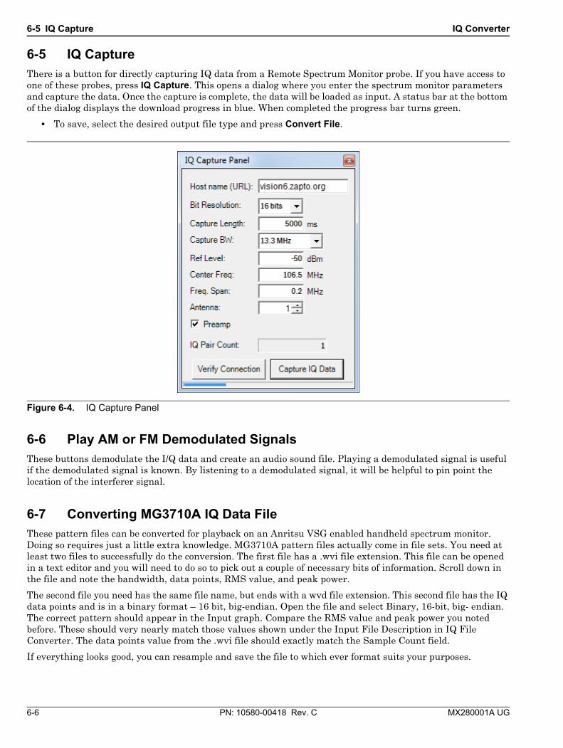
6-5 IQ Capture IQ Converter

6-6 PN: 10580-00418 Rev. C MX280001A UG

6-5 IQ CaptureThere is a button for directly capturing IQ data from a Remote Spectrum Monitor probe. If you have access to one of these probes, press IQ Capture. This opens a dialog where you enter the spectrum monitor parameters and capture the data. Once the capture is complete, the data will be loaded as input. A status bar at the bottom of the dialog displays the download progress in blue. When completed the progress bar turns green.

• To save, select the desired output file type and press Convert File.

6-6 Play AM or FM Demodulated SignalsThese buttons demodulate the I/Q data and create an audio sound file. Playing a demodulated signal is useful if the demodulated signal is known. By listening to a demodulated signal, it will be helpful to pin point the location of the interferer signal.

6-7 Converting MG3710A IQ Data FileThese pattern files can be converted for playback on an Anritsu VSG enabled handheld spectrum monitor. Doing so requires just a little extra knowledge. MG3710A pattern files actually come in file sets. You need at least two files to successfully do the conversion. The first file has a .wvi file extension. This file can be opened in a text editor and you will need to do so to pick out a couple of necessary bits of information. Scroll down in the file and note the bandwidth, data points, RMS value, and peak power.

The second file you need has the same file name, but ends with a wvd file extension. This second file has the IQ data points and is in a binary format – 16 bit, big-endian. Open the file and select Binary, 16-bit, big- endian. The correct pattern should appear in the Input graph. Compare the RMS value and peak power you noted before. These should very nearly match those values shown under the Input File Description in IQ File Converter. The data points value from the .wvi file should exactly match the Sample Count field.

If everything looks good, you can resample and save the file to which ever format suits your purposes.

Figure 6-4. IQ Capture Panel

Anritsu utilizes recycled paper and environmentally conscious inks and toner.

Anritsu Company490 Jarvis Drive

Morgan Hill, CA 95037-2809USA

http://www.anritsu.com