
Research on Brain-inspired Vision Based on Dynamic Vision ...

Vision Research 48 (2008) 1345–1373
Contents lists available at ScienceDirect
Vision Research
journal homepage: www.elsevier .com/locate /v isres
Temporal dynamics of decision-making during motion perceptionin the visual cortex
Stephen Grossberg *, Praveen K. Pilly 1
Department of Cognitive and Neural Systems, Center for Adaptive Systems, Center of Excellence for Learning in Education, Science, and Technology, Boston University,677 Beacon Street, Boston, MA 02215, USA
a r t i c l e i n f o
Article history:Received 23 July 2007Received in revised form 19 February 2008
Keywords:Motion perceptionDirection discriminationDecision-makingVisual cortexAperture problemMotion captureNoise-saturation dilemmaRecurrent competitive fieldBayesian inferenceStochastic decision modelsDiffusion modelsSpeed–accuracy trade-offShunting modelOn-center off-surround networkMTMSTLIPBasal gangliaPsychometric function
0042-6989/$ - see front matter � 2008 Elsevier Ltd. Adoi:10.1016/j.visres.2008.02.019
* Corresponding author. Fax: +1 617 353 7755.E-mail addresses: [email protected] (S. Grossberg), adv
1 Authorship in alphabetical order. S.G. was suppoScience Foundation (NSF SBE-0354378), and the OfN00014-01-1-0624). P.K.P. was supported in part by th(NIH R01-DC-02852), the National Science FoundationSBE-0354378), and the Office of Naval Research (ONR
a b s t r a c t
How does the brain make decisions? Speed and accuracy of perceptual decisions covary with certainty inthe input, and correlate with the rate of evidence accumulation in parietal and frontal cortical ‘‘decisionneurons”. A biophysically realistic model of interactions within and between Retina/LGN and corticalareas V1, MT, MST, and LIP, gated by basal ganglia, simulates dynamic properties of decision-makingin response to ambiguous visual motion stimuli used by Newsome, Shadlen, and colleagues in theirneurophysiological experiments. The model clarifies how brain circuits that solve the aperture probleminteract with a recurrent competitive network with self-normalizing choice properties to carry out prob-abilistic decisions in real time. Some scientists claim that perception and decision-making can bedescribed using Bayesian inference or related general statistical ideas, that estimate the optimal interpre-tation of the stimulus given priors and likelihoods. However, such concepts do not propose the neocor-tical mechanisms that enable perception, and make decisions. The present model explains behavioral andneurophysiological decision-making data without an appeal to Bayesian concepts and, unlike other exist-ing models of these data, generates perceptual representations and choice dynamics in response to theexperimental visual stimuli. Quantitative model simulations include the time course of LIP neuronaldynamics, as well as behavioral accuracy and reaction time properties, during both correct and error tri-als at different levels of input ambiguity in both fixed duration and reaction time tasks. Model MT/MSTinteractions compute the global direction of random dot motion stimuli, while model LIP computes thestochastic perceptual decision that leads to a saccadic eye movement.
� 2008 Elsevier Ltd. All rights reserved.
1. Introduction
The brain’s ability to carry out context-appropriate perceptuallybased decisions in response to ambiguous and probabilistic situa-tions plays an essential role in ensuring animal and human sur-vival. How the speed and accuracy of decisions varies with theambiguity of environmental information is of particular interest(Gold & Shadlen, 2007; Luce, 1986).
ll rights reserved.
[email protected] (P.K. Pilly).rted in part by the National
fice of Naval Research (ONRe National Institutes of Health
(NSF IIS-02-05271 and NSFN00014-01-1-0624).
A valuable paradigm for studying decision-making, which linkspsychophysics and neurophysiology, has been developed by New-some, Shadlen, and colleagues (Roitman & Shadlen, 2002; Shadlen& Newsome, 2001). This research studies how brain dynamics inlateral intraparietal (LIP) area relate to saccadic behavior of mon-keys (% accuracy, reaction time), that are based upon discriminat-ing the motion direction of random dot motion stimuli at variousdegrees of coherence.
In these experiments, two kinds of tasks were employed: fixedduration (FD) and reaction time (RT) tasks. Macaques weretrained to discriminate net motion direction and report it via asaccade. Random dot motion displays, covering a 5� diameteraperture centered at the fixation point on a computer monitor,were used to control motion coherence; namely, the fraction ofdots moving non-randomly in a particular direction from oneframe to the next in each of the three interleaved sequences(see Appendix A.1 for details about the motion algorithm).

1346 S. Grossberg, P.K. Pilly / Vision Research 48 (2008) 1345–1373
Varying the motion coherence provides a quantitative way tomanipulate the ambiguity of directional information that themonkey uses to make a saccadic eye movement to a peripheralchoice target in the judged motion direction, and thus the taskdifficulty. More coherence resulted in better accuracy and fasterresponses.
In the FD task (Roitman & Shadlen, 2002; Shadlen & Newsome,2001), monkeys viewed the moving dots for a fixed duration of 1 s,and then made a saccade to the target in the judged direction aftera variable delay. In the RT task (Roitman & Shadlen, 2002), mon-keys had theoretically unlimited viewing time, and were trainedto report their decision as soon as the motion direction was deter-mined. The RT task allowed measurement of how long it took themonkey to make a decision, which was defined as the time fromthe onset of the motion until when the monkey initiated a saccade.The two monkeys in the Roitman and Shadlen (2002, p. 9476) wereshaped during RT task training to initiate the choice saccade within‘‘�1 s” after the dots turn on. In each RT task trial, the monkeys hadto wait for a minimum of about 1 s (one monkey: 800 ms, and theother: 1200 ms) after motion onset to receive a reward howeverrapidly they responded. Human subjects in a similar RT task usu-ally respond around 1 s from motion onset for the weakest coher-ence without any speed instruction (Palmer, Huk, & Shadlen, 2005,p. 385).
Neurophysiological recordings were done in LIP while themonkeys performed these tasks. The recorded neurons had recep-tive fields (RF) that encompassed just one target, and did not in-clude the circular aperture in which the moving dots weredisplayed. Also, they were among those that showed sustainedactivity during the delay period in a memory-guided saccade task.It was found that the speed and accuracy of perceptual decisionscovaried strongly with the rate of evidence accumulation in LIPcells.
Several authors (Gold & Shadlen, 2001, 2007; Jazayeri & Movs-hon, 2006; Ma, Beck, Latham, & Pouget, 2006; Rao, 2004) have sug-gested that these data illustrate Bayesian inference in the brain.Indeed, Gold and Shadlen (2001) have suggested that the ‘‘loga-rithm of the likelihood ratio (logLR) provides a natural currencyfor trading off sensory information, prior probability and expectedvalue to form a perceptual decision” (p. 10). See Section 4.2 fortheir proposal. Despite their intuitive appeal, Bayesian modelsheretofore have not processed the perceptual stimuli that wereused in the experiments, and have not disclosed novel brain mech-anisms of decision-making.
Non-Bayesian models for the above dataset also exist (Ditterich,2006a, 2006b; Mazurek, Roitman, Ditterich, & Shadlen, 2003;Wang, 2002), but none of them clarifies how the perceptual ambi-guity that is created by the randomly moving dots is graduallytransformed by the brain into a perceptual decision in responseto the non-randomly moving dots. In particular, previous modelshave missed important brain principles and mechanisms that areat play in the dots task by ignoring the motion processing that ex-tracts a dynamic neural representation of the directional uncer-tainty inherent in the random dot motion stimulus. They modeldecision-making properties only after assuming that the neuralcode of sensory uncertainty is provided. Section 4.3 details similar-ities and differences between our model and previous work in thefield.
We here show how the data may be quantitatively simulated bya biophysically realistic model of interactions within and betweenRetina/LGN and cortical areas V1, MT, MST, and LIP, gated by basalganglia (BG). The model achieves these results when it is directlyactivated by the visual stimuli that were used in the experiments(Fig. 1). Our results have been briefly reported in Pilly and Gross-berg (2005, 2006). These model circuits solve two general designproblems that are faced by the brain.
The aperture problem (Wallach, 1935) occurs whenever objectsmove with respect to spatially limited receptive fields of neurons:how can an unambiguous direction and speed of global object mo-tion be determined from local motion signals that are ambiguousat most locations on the object?
The noise-saturation problem (Grossberg, 1973, 1980) occurswithin all neurons because their activations fluctuate within asmall interval of possible values: how does a network of cells, orcell populations, remain sensitive to the spatially distributed pat-tern of their inputs as they vary greatly in size through time? Aspecial case of such networks shows how the most highly activatedcell, or cell population, is selected to make a decision.
Our model’s successful simulations of perceptual decision-mak-ing data support the hypothesis that the brain designs which solvethe aperture problem and noise-saturation problem also underlieperceptual decision-making during random dot motion directiondiscrimination tasks. Individual moving dots do not experiencethe aperture problem. However, we claim that principles andmechanisms that have evolved in the brain to tackle the apertureproblem can also help us intuitively understand the data at hand.The aperture problem is faced by any localized neural motion sen-sor, such as a neuron in the early visual pathway, which respondsto a local contour moving through its aperture-like receptive field.Only when the contour within the aperture contains features, suchas line terminators, object corners, junctions, high contrast blobs,or dots, can the local motion detector accurately signal the direc-tion and speed of motion.
For example, the direction of motion of a featureless straightline seen behind an occluding aperture is thus ambiguous. Whenthe aperture is circular, the line seems to move perpendicular toits orientation. When the aperture is rectangular, as during the bar-berpole illusion (Wallach, 1935), moving lines may appear to movein the direction parallel to the longer edges of the rectangle withinwhich they move, even if their actual motion direction is not par-allel to these edges. The brain must solve this problem in order todetect the correct motion directions of important moving objectsin the world.
To overcome aperture ambiguities, the visual cortex embodiestwo complementary processes of motion integration and motionsegmentation. The former process joins nearby motion signals intoa single object, while the latter keeps them separate as belongingto different objects. The visual cortex uses the relatively few unam-biguous motion signals arising from image features, called featuretracking signals, to inhibit the more numerous ambiguous signalsfrom contour interiors. For example, during the barberpole illusion,feature tracking signals from the moving line ends along the longeredges of the bounding rectangle of the barberpole compute anunambiguous motion direction. These feature tracking signalsgradually propagate into the interior of the rectangle. This motioncapture process selects the feature tracking motion direction fromthe possible ambiguous directions along the lines within the rect-angle, and suppresses the ambiguous motion signals correspond-ing to other directions that are generated by the moving lines(Ben-Av & Shiffrar, 1995; Bowns, 1996, 2001; Castet, Lorenceau,Shiffrar, & Bonnet, 1993; Chey, Grossberg, & Mingolla, 1997,1998; Grossberg, Mingolla, & Viswanathan, 2001; Lorenceau &Gorea, 1989; Mingolla, Todd, & Norman, 1992). When a scene doesnot contain any unambiguous motion signals, the ambiguous mo-tion signals cooperate to compute a consistent object motion direc-tion and speed (Grossberg et al., 2001; Lorenceau & Shiffrar, 1992).
The brain thus needs to ensure that a sparse set of unambiguousfeature tracking motion signals can gradually capture a greaternumber of ambiguous motion signals to determine the globaldirection and speed of object motion. In the case of random dotmotion discrimination tasks, the signal dots at any coherence levelproduce locally unambiguous, though short-lived, motion signals.

PRIMING
SACCADIC TARGET SELECTION (LIP)
DIRECTIONAL SHORT-RANGE FILTER
DIRECTIONAL TRANSIENT CELL
SPATIAL AND OPPONENT DIRECTIONAL COMPETITION
DIRECTIONAL LONG-RANGE FILTER (MT)
DIRECTIONAL GROUPING NETWORK (MSTv)
PRIMING (DLPFC)
NON-DIRECTIONAL TRANSIENT CELL
CONTEXTUAL GATING (BG)
Local directional signals
Evidence accumulation amplifies feature tracking (FT) signals
FT signals are strengthened, ambiguous signals weakened
Pools signals over multiple orientations, opposite contrast polarities, both eyes, multipledepths, and a larger spatial scale
A winning direction is chosen and fed back to MT
Choice of saccadic response
Contextual gating of response
Fig. 1. Retina/LGN–V1–MT–MST–LIP–BG model processing stages. See text and Appendix for details.
S. Grossberg, P.K. Pilly / Vision Research 48 (2008) 1345–1373 1347
The model shows how the same brain circuits that help resolve theaperture problem can also enable a small number of coherentlymoving dots to capture, as much as possible, the random motiondirections caused by a large number of unambiguous, but incoher-ently moving, dots.
2. Model
Model processing stages are summarized in Fig. 1. Model equa-tions and parameters are provided in Appendix A. The motion pro-cessing stages of the model were adapted from the MotionBoundary Contour System (mBCS) model, which clarifies how cor-tical areas V1, MT, and MST interact together to solve the apertureproblem and create the brain’s best representation of object mo-tion direction and speed (Berzhanskaya, Grossberg, & Mingolla,2007; Chey et al., 1997; Grossberg et al., 2001). The output fromMST in the mBCS model is thus a perceptual representation thatis not in the correct coordinates to command eye or arm move-ments towards a goal object.
The Motion Decision BCS (mdBCS) model, also known forshort as the MOtion DEcision (MODE) model, that is developedherein adds an LIP decision-making circuit that discriminatesmotion direction based on inputs from the distributed motionrepresentation of the model MST processing stage, and is gatedby a simplified basal ganglia circuit. This enhanced model con-verts random dot motion stimuli into stochastic directionalmovement commands that are sensitive to the amount of direc-tional coherence in the stimuli. The model processing stages areas follows.
2.1. Motion processing by V1, MT, and MST
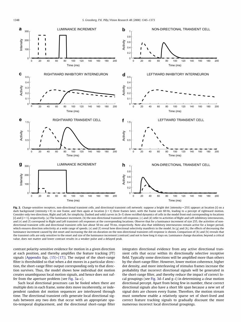
The model change-sensitive receptors, non-directional transientcells and directional transient cells, compute local directional sig-nals in response to image random dot motion. In particular, when-ever a dot shows up at a spatial location, after being eitherrandomly relocated or moved by a fixed displacement in the signaldirection, a non-directional transient pulse is elicited at that loca-tion (see Appendix Eqs. (9)–(11)). This feeds into a directional tran-sient cell network (Appendix Eqs. (12)–(14)) where local directionalsignals are computed. For example, suppose a dot arrives at location[i + 1] from the leftward location [i]. Then the rightward inhibitoryinterneuron at location [i] inhibits the leftward inhibitory interneu-ron and transient cell at location [i + 1] well enough that they can-not recover to above-baseline firing when the dot does arrive atlocation [i + 1] a little later (cf., Barlow & Levick, 1965). As a result,the leftward transient response is not obtained (see Fig. 2). Otherdirectional transient cells at location [i + 1] may be activated if theyare not similarly inhibited in advance by their corresponding nulldirection interneuron at the location which is one unit from [i + 1]in the preferred direction (see Appendix A.3.2 and Fig. 3a and b).In addition, directional inhibitory interneurons preserve directionsensitivity at a wide range of motion speeds. Appendix A.3.2 notesthat these interneurons may be compared with starburst amacrinecells (Appendix Eq. (12)) and thus predicts that starburst cells mayhelp transient cells to retain their directional sensitivity in responseto motion at variable speeds.
The directional transient cell output signals feed into the direc-tional short-range filter in V1, which accumulates monocular and
0 20 40 60 80 100 120 140 160 180 2000
100
200
300
0 20 40 60 80 100 120 140 160 180 2000
0.2
0.4
0.6
0.8
1
0 20 40 60 80 100 120 140 160 180 2000
0.1
0.2
0.3
0.4
0.5
0 20 40 60 80 100 120 140 160 180 2000
0.1
0.2
0.3
0.4
0.5
0 20 40 60 80 100 120 140 160 180 2000
0.5
1
1.5
0 20 40 60 80 100 120 140 160 180 2000
0.5
1
1.5
0 20 40 60 80 100 120 140 160 180 2000
100
200
300
0 20 40 60 80 100 120 140 160 180 2000
0.2
0.4
0.6
0.8
1
Inte
nsity
Activ
ityAc
tivity
Activ
ityAc
tivity
Activ
ityAc
tivity
Inte
nsity
LUMINANCE INCREMENT NON-DIRECTIONAL TRANSIENT CELL
RIGHTWARD INHIBITORY INTERNEURON LEFTWARD INHIBITORY INTERNEURON
RIGHTWARD TRANSIENT CELL LEFTWARD TRANSIENT CELL
LUMINANCE INCREMENT NON-DIRECTIONAL TRANSIENT CELL
Time (ms)
Time (ms)
Time (ms)
Time (ms)
Time (ms) Time (ms)
Time (ms) Time (ms)
Fig. 2. Change-sensitive receptors, non-directional transient cells, and directional transient cell network: suppose a bright dot (intensity = 255) appears at location [i] on adark background (intensity = 0) in one frame, and then again at location [i + 1] three frames later, with the frame rate 60 Hz, leading to a percept of rightward motion.Consider only two directions, Right and Left, for simplicity. Dashed and solid curves in (b–f) show rectified dynamics of cells in the model front end corresponding to locations[i] and [i + 1], respectively. (a) The luminance increment, (b) the non-directional transient cell response, (c) and (d) refer to activities of Right and Left inhibitory interneurons,and (e) and (f) correspond to Right and Left transient cell responses at the corresponding locations. Observe that for a luminance increment of size 255, the activities of non-directional transient cells and directional transient cells last about 50 ms and 70 ms, respectively. Note also that inhibitory interneurons remain active for a longer period,which ensures direction selectivity at a wide range of speeds. (e) and (f) reveal how directional selectivity manifests in the model. In (g) and (h), the effects of decreasing theluminance increment caused by dot onset and increasing the dot on-duration on the non-directional transient cell response is shown. Comparison of (h) and (b) reveals thatthe transient cells are only sensitive to the onset and size of the luminance increment (contrast) and not to how long it stays on. Luminance change duration, beyond a criticalvalue, does not matter and lower contrast results in a weaker pulse and a delayed peak.
1348 S. Grossberg, P.K. Pilly / Vision Research 48 (2008) 1345–1373
contrast polarity-sensitive evidence for motion in a given directionat each position, and thereby amplifies the feature tracking (FT)signals (Appendix Eqs. (15)–(17)). The output of the short-rangefilter is thresholded so that when a dot moves in a particular direc-tion, the short-range filter output corresponding only to that direc-tion survives. Thus, the model shows how individual dot motioncreates unambiguous local motion signals, and hence does not suf-fer from the aperture problem (see Fig. 3a–c).
Such local directional processes can be fooled when there aremultiple dots in each frame, some dots move incoherently, or inde-pendent random dot motion sequences are interleaved throughtime. The directional transient cells generate local directional sig-nals between any two dots that occur with an appropriate spa-tio-temporal displacement, and the directional short-range filter
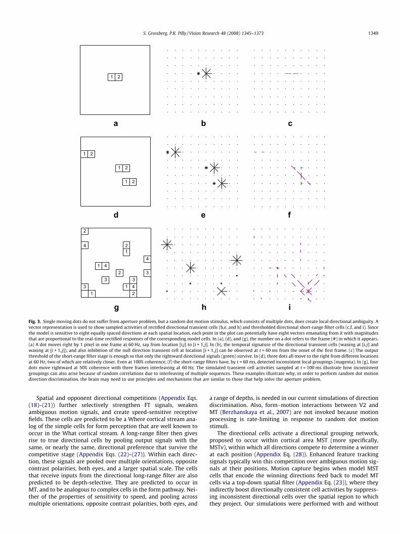
integrates directional evidence from any active directional tran-sient cells that occur within its directionally selective receptivefield. Typically some directions will be amplified more than othersby the short-range filter. However, lower motion coherence, higherdot density, and more interleaving of stimulus frames increase theprobability that incorrect directional signals will be generated inthe short-range filter, and thereby reduce the impact of correct lo-cal groupings (see Fig. 3d–f and g–i) in determining a clear motiondirectional percept. Apart from being few in number, these correctdirectional signals also have a short life span because a new set ofsignal dots are chosen every frame. Therefore, the motion streammust somehow enable a relatively sparse set of short-lived andcorrect feature tracking signals to gradually discount the morenumerous incorrect local directional groupings.
1 2
1 2
1 2
1 2
1
1
11
2
2
2
23
3 33
4
4
4
4
a b c
d e f
g h iFig. 3. Single moving dots do not suffer from aperture problem, but a random dot motion stimulus, which consists of multiple dots, does create local directional ambiguity. Avector representation is used to show sampled activities of rectified directional transient cells (b,e, and h) and thresholded directional short-range filter cells (c,f, and i). Sincethe model is sensitive to eight equally spaced directions at each spatial location, each point in the plot can potentially have eight vectors emanating from it with magnitudesthat are proportional to the real-time rectified responses of the corresponding model cells. In (a), (d), and (g), the number on a dot refers to the frame (#) in which it appears.(a) A dot moves right by 1 pixel in one frame at 60 Hz, say from location [i,j] to [i + 1, j]. In (b), the temporal signature of the directional transient cells (waning at [i, j] andwaxing at [i + 1, j]), and also inhibition of the null direction transient cell at location [i + 1, j] can be observed at t = 60 ms from the onset of the first frame. (c) The outputthreshold of the short-range filter stage is enough so that only the rightward directional signals (green) survive. In (d), three dots all move to the right from different locationsat 60 Hz, two of which are relatively closer. Even at 100% coherence, (f) the short-range filters have, by t = 60 ms, detected inconsistent local groupings (magenta). In (g), fourdots move rightward at 50% coherence with three frames interleaving at 60 Hz. The simulated transient cell activities sampled at t = 100 ms illustrate how inconsistentgroupings can also arise because of random correlations due to interleaving of multiple sequences. These examples illustrate why, in order to perform random dot motiondirection discrimination, the brain may need to use principles and mechanisms that are similar to those that help solve the aperture problem.
S. Grossberg, P.K. Pilly / Vision Research 48 (2008) 1345–1373 1349
Spatial and opponent directional competitions (Appendix Eqs.(18)–(21)) further selectively strengthen FT signals, weakenambiguous motion signals, and create speed-sensitive receptivefields. These cells are predicted to be a Where cortical stream ana-log of the simple cells for form perception that are well known tooccur in the What cortical stream. A long-range filter then givesrise to true directional cells by pooling output signals with thesame, or nearly the same, directional preference that survive thecompetitive stage (Appendix Eqs. (22)–(27)). Within each direc-tion, these signals are pooled over multiple orientations, oppositecontrast polarities, both eyes, and a larger spatial scale. The cellsthat receive inputs from the directional long-range filter are alsopredicted to be depth-selective. They are predicted to occur inMT, and to be analogous to complex cells in the form pathway. Nei-ther of the properties of sensitivity to speed, and pooling acrossmultiple orientations, opposite contrast polarities, both eyes, and
a range of depths, is needed in our current simulations of directiondiscrimination. Also, form–motion interactions between V2 andMT (Berzhanskaya et al., 2007) are not invoked because motionprocessing is rate-limiting in response to random dot motionstimuli.
The directional cells activate a directional grouping network,proposed to occur within cortical area MST (more specifically,MSTv), within which all directions compete to determine a winnerat each position (Appendix Eq. (28)). Enhanced feature trackingsignals typically win this competition over ambiguous motion sig-nals at their positions. Motion capture begins when model MSTcells that encode the winning directions feed back to model MTcells via a top-down spatial filter (Appendix Eq. (23)), where theyindirectly boost directionally consistent cell activities by suppress-ing inconsistent directional cells over the spatial region to whichthey project. Our simulations were performed with and without
1350 S. Grossberg, P.K. Pilly / Vision Research 48 (2008) 1345–1373
internal cellular noise in both MT and MST in order to assess theeffects of such noise on the model’s stochastic decision-making.
This shift in the spatial locus of unambiguous feature trackingsignals continues to propagate across space as the MST-to-MTfeedback process cycles through time. The action of this feedbackloop was predicted to solve the aperture problem, and to generatea representation of global object direction and speed (Berzhans-kaya et al., 2007; Chey et al., 1997; Grossberg et al., 2001). Packand Born (2001) have reported neurophysiological data which sup-port this prediction.
The rate and strength of motion capture by the MT/MST feed-back loop is reflected in the decision-making properties of modelLIP, as it receives its inputs from MST. Model LIP hereby simulatesthe temporal dynamics of decision-making in the neurophysiologi-cal and behavioral data. The intuitive idea is that the feedback loopneeds more time to capture the incoherent motion signals, andcannot achieve as high a level of asymptotic response magnitude,when there are more of them competing with the emerging win-ning direction. A key point of this article is thus that the effective-ness of the motion capture process depends on the input coherenceand exposure duration. LIP converts the spatially distributed direc-tional motion signals from MST into an eye movement command,in the manner noted below, and thereby enables the monkey to re-port its decision via a saccade.
2.2. Probabilistic decision-making by LIP with BG gating
As noted above, the motion information from the model MSTstage (Fig. 1) is spatially distributed and needs to be converted intoa form where it can command an eye movement to the choice tar-get that corresponds to the judged net motion direction. These tar-gets are present at a specific eccentricity in the respectivedirections of the motion during both the training and the recordingphases of the experiments. In these experiments, LIP cells do exhi-bit decision-related activity that correlates with a saccadic eyemovement to one of the two or more possible choice targets. Themodel LIP circuit (see Appendix Eqs. (29)–(34)) converts the spa-tially distributed directional motion signals into the activation ofcells that code for saccadic eye movements in specific directions.
This LIP circuit is modeled using a kind of decision circuit thathas become classical in the neural modeling literature; namely anetwork of cells that obey membrane equation, or shunting,dynamics and interact via a recurrent on-center off-surround net-work (Grossberg, 1973, 1980). Such a network is often called arecurrent competitive field (RCF), and its variants have been usedby a number of authors to model the dynamics of perceptual ormotor decisions in both deterministic models (e.g., Brown, Bullock,& Grossberg, 2004; Chey et al., 1997; Francis, Grossberg, & Mingo-lla, 1994; Francis & Grossberg, 1996a, 1996b) and stochastic mod-els (Boardman, Grossberg, Myers, & Cohen, 1999; Cisek, 2006;Grossberg, Boardman, & Cohen, 1997; Grossberg & Myers, 2000;Usher & McClelland, 2001). It should be noted that even a deter-ministic RCF typically describes the temporal evolution of popula-tion mean activities and cell firing frequencies. It is only whenproperties that depend upon the variance of cell firing becomerate-limiting that explicit noise terms add explanatory power.
There is another sense in which RCFs, and indeed all shuntingon-center off-surround models, embody probabilistic properties.The shunting dynamics of a RCF lead to automatic gain controland self-normalizing properties, so that the total activity of a pro-cessing channel in such a model is often approximately conserved.This total activity plays the role of a real-time probability distribu-tion. Self-normalization enables such a network to maintain itssensitivity in response to distributed inputs whose total numberand size can vary wildly through time. This property is useful whenestimating the directional coherence of inputs whose total number
and distribution can vary randomly through time, as occurs in theexperiments that are simulated in this article. This robustness isillustrated by the fact that model properties remain qualitativelyunchanged when cellular noise is added to MT and MST, as illus-trated in Fig. 15.
The RCF that models LIP herein has the following properties (seeFig. 4 and Appendix Eqs. (29) and (34)):
(1) Each cell activity (yd) corresponding to movement directiond in the LIP RCF is associated with the peripheral choice tar-get within its response field.
(2) Each LIP cell gets excited by the spatially distributed popula-tion activity of the foveal MST pool of neurons coding its pre-ferred motion direction (see term Sd in Appendix Eqs. (29)and (34)). It is assumed that these pro-saccade connectionsare gradually strengthened as a result of extensive operantconditioning on the task. As a result, each cell’s activity pre-dicts that the global motion of the random dots is in thedirection from the fovea to its choice target.
(3) Each cell also receives a bottom-up excitatory input due tothe presence of a choice target within its response field(see term TC in Appendix Eqs. (29) and (34)). This input pro-duces the above-baseline activity observed before the onsetof the dots.
(4) Each cell receives recurrent self-excitation (f(yd)) via a sig-moidal signal function, and recurrent inhibition (h(yD)) fromother cells via another sigmoidal signal function (Grossberg,1973, 1980).
(5) Each LIP cell is subject to an individual internal noise processthat influences stochastic choice dynamics (see term W inAppendix Eqs. (29) and (34)). A similar hypothesis has beenused to quantitatively simulate the temporal dynamics ofspeech categorization data (Boardman et al., 1999; Gross-berg, Boardman, et al., 1997; Grossberg & Myers, 2000). Thisnoise process contributes to the known variability in theread-out from sensory to motor areas. Model simulationsshow that the LIP cellular noise, in combination with therandomness of the moving dot stimuli, can explain the var-iability in saccadic decision-making, whether or not there isnoise at the MT and MST processing stages.
(6) During the RT task, when one of the competing LIP cells firstreaches a fixed decision threshold (C1), a directional decisionis initiated by opening a basal ganglia (BG) movement gatethat increases the gain of the corresponding cell’s self-exci-tation (see gd in Appendix Eq. (29)) to a high value (see gBG
in Appendix A.3.6). This event triggers the final stage of LIPfiring, namely pre-saccadic enhancement that is indepen-dent of motion coherence. LIP hereby transitions from thesensory mode to the motor mode. All LIP cells continue tointegrate their sensory inputs, but the selected cell popula-tion does so at a higher self-excitatory gain. A saccade tothe associated target is initiated when the winning cell’s fir-ing rate reaches a criterion level (C2). The reaction time (RT)is the time from stimulus onset to when the choice saccadeis made, not the time when the decision is initiated. Bothdecision time and RT are emergent properties, and covarywith each other.
(7) As noted in Section 1, Roitman and Shadlen (2002) delayedreward until �1 s after motion onset during RT task training.During the RT task, mostly during weaker coherence trials,cells in the RCF may take longer than 1 s to reach the deci-sion threshold. If none of the activities sampled at a randomtime between 1000 and 1100 ms has crossed the decisionthreshold (see term Gd in Appendix Eq. (29)), then a voli-tional top-down signal boosts the LIP cell with the largestactivity. A choice made in this manner is termed a ‘‘forced

L R
BGL BGR
NOISENOISE
Fovea PeripheryPeriphery
MST
LIP
Fig. 4. Components of the LIP decision circuit. The activities of the cells in the recurrent competitive field predict the perceptual decision regarding the direction of therandomly moving dots. Each cell receives two bottom-up inputs: one from the form stream due to the presence of the peripheral choice target (indicated by a small circle) inthe response field, and the other from the foveal MST pool of the motion stream tuned to its preferred direction. The latter sensory input comes from outside the responsefield. This non-classical neural connection is thought to result from training on the stereotypical task. Also, each cell self-excites itself and is inhibited by other competing cellsin the field via different sigmoidal signal functions, which are indicated on the respective connections. The gain of the recurrent self-excitation is regulated by the basalganglia. Two time-appropriate top-down inputs, an inhibitory one that simulates post-saccadic suppression, and an excitatory one that helps the decision circuit make aforced choice in trials of extended uncertainty, are not depicted. Internal noise processes to each cell help to simulate the probabilistic nature of perceptual decisions.
S. Grossberg, P.K. Pilly / Vision Research 48 (2008) 1345–1373 1351
choice”. Section 3.2 cites evidence that support this hypoth-esis. The model monkey is also simulated without this voli-tional mechanism, and can still make coherence-sensitivechoices, but some longer RTs are generated as a result.
(8) Cell activities decay faster in the FD task, in keeping with theexperimental observation that the gain of the LIP response issmaller in the FD task than in the RT task (Roitman & Shad-len, 2002, p. 9485), and also that LIP responses tend to satu-rate during the viewing duration in the FD task.
(9) During the FD task, at the end of the viewing duration of 1 s,the model chooses the motion direction corresponding tothe maximally active LIP cell, by increasing the self-excit-atory gain of this cell (see term gdelay in Appendix A.3.6). Thisevent causes a persistent and slow buildup activity duringthe variable delay period after the input from motion areasshuts off. The basal ganglia increase this gain further (termgd in Appendix Eq. (34) jumps to gBG), resulting in coher-ence-independent pre-saccadic enhancement, as in the RTtask.
(10) After a saccade begins, all LIP cells receive a strong inhibitorysignal. In vivo, the source of this signal is possibly from fron-tal eye field (FEF) post-saccadic cells (Brown et al., 2004;Bruce, Goldberg, Bushnell, & Stanton, 1985) (see term GI inAppendix Eqs. (29) and (34)).
Section 3 discusses in detail how these LIP RCF properties helpto explain the simulated data.
3. Results
3.1. Data summary
The recorded LIP neurons show visuo-motor responses. Theyhave properties of both buildup and burst cells (Munoz & Wurtz,
1995a) that are found in superior colliculus (SC). First, visual tar-gets present in the receptive fields contribute to above-baselineLIP firing before the dots turn on. Even though the motion stimulusis not presented within their classical receptive fields, these neu-rons still respond with direction selectivity, probably because ofextensive training on the tasks during which new stimulus–re-sponse associations are learned (Bichot & Schall, 1996). This prop-erty has also been observed for SC neurons in monkeys trained toperform an FD task (Horwitz, Batista, & Newsome, 2004a; Horwitz& Newsome, 2001a).
On correct trials during the decision-making period, morecoherence in the preferred direction causes faster LIP cell activa-tion, on average, in both the tasks (Fig. 5), and also higher maximalcell activation in the FD task (Fig. 5c–f). More coherence in theopposite direction causes faster cell inhibition in both the tasks,and also lower minimal cell activation in the FD task. Thus on cor-rect trials, the instantaneous difference in average LIP activity be-tween judgments of net motion being towards the receptive field(Tin choices) and judgments of motion being away from the recep-tive field (Tout choices) increases with coherence. In other words,the correct trial predictiveness of LIP cell responses is proportionalto % coherence.
The temporal dynamics of LIP decision neurons also correlatewith behavioral properties of perceptual decision-making (Fig. 6).In both FD and RT tasks, more coherence in the motion translatesinto more accurate decisions (Fig. 6a and b). Also, RT task accuracyat weaker coherence levels is slightly better than FD task accuracy.The psychometric function ranges from about chance level to 100%accuracy as the dot coherence varies from 0% to 100%, respectively.In addition, a longer viewing duration in the FD task tends to im-prove performance at all motion strengths (Fig. 2A and B in Gold& Shadlen, 2003), revealing a speed–accuracy trade-off (Fig. 7)wherein performance asymptotes at shorter durations for highercoherences. More coherence also results in faster reaction times

Fig. 5. Temporal dynamics of LIP neuronal responses during the fixed duration (FD) and reaction time (RT) tasks. (a) Average responses of a population of 54 LIP neuronsamong correct trials during the RT task (Roitman & Shadlen, 2002). The left part of the plot is time-aligned to the motion onset, and includes activity only up to the median RT,and excludes any activity within 100 ms backward from saccade initiation (which roughly corresponds to pre-saccadic enhancement in firing). The right part of the plot istime-aligned to the saccade initiation, and excludes any activity within 200 ms forward from motion onset (which corresponds to initial transient pause in firing). (b) Modelsimulations replicate LIP cell recordings during the RT task. In both data and simulations for the RT task, the average responses were smoothed with a 60 ms running mean. (c)Average responses of a population of 38 LIP neurons among correct trials during the 2002 FD task (Roitman & Shadlen, 2002), during both the motion viewing period (1 s) anda part (0.5 s) of the delay period before the saccade is made. (d) Model simulations mimic LIP cell recordings during the 2002 FD task. (e) Average responses of a population of104 LIP neurons among correct trials during the 2001 FD task (Shadlen & Newsome, 2001), during both the motion viewing period (1 s) and a part (0.5 s) of the delay periodbefore the saccade is made. (f) Model simulations emulate LIP cell recordings during the 2001 FD task. In (a–f), solid and dashed curves correspond to trials in which themonkey correctly chose the right target (Tin) and the left target (Tout), respectively. Cell dynamics (rate of rise or decline, and response magnitude) reflect the incomingsensory ambiguity (note the different colors; the color code for the various coherence levels is shown in the corresponding data panels), and the perceptual decision (solid: Tin
choices, dashed: Tout choices). Note that for 0% coherence, even though there is no correct choice per se, the average LIP response rose or declined depending on whether themonkey chose Tin or Tout, respectively. [Data in (a,c) and (e) is reprinted with permission from Roitman and Shadlen (2002) and Shadlen and Newsome (2001), respectively.]
1352 S. Grossberg, P.K. Pilly / Vision Research 48 (2008) 1345–1373
in the RT task (Fig. 6c and d). Moreover, the monkey responds withrelatively slower reaction times on error trials when compared tocorrect trials. Reaction time standard errors of mean (SEM) de-crease with coherence on correct trials, and increase with coher-
ence on error trials. Error trial SEMs are greater than those forcorrect trials (Table 2 in Roitman & Shadlen, 2002).
Cell responses on error trials and 0% coherence trials duringboth FD and RT tasks reveal that LIP firing reflects the perceptual

1 1050
100
Motion strength (% coherence)
Accu
racy
(% c
orre
ct)
1 10 100400
500
600
700
800
900
1000
Motion strength (% coherence)
Rea
ctio
n tim
e (m
s)
1 10 100400
500
600
700
800
900
1000
Motion strength (% coherence)
Rea
ctio
n tim
e (m
s)
0 0
Fig. 6. Psychometric and chronometric data during the FD and RT tasks (Roitman & Shadlen, 2002). (a) Accuracy data (% correct) as a function of motion coherence (% certainty) isfit using a cumulative Weibull distribution function for both FD and RT tasks (Fig. 6B in Mazurek et al., 2003). The ability to discriminate motion direction depends on the stimulusstrength. Accuracy in the RT task is slightly better than that in the FD task for lower coherence levels. (b) Model simulations emulate these data. Solid curve corresponds to the RTtask, and dashed curve to the 1s FD task. Number of trials is 500. The two parameters, a (threshold) and b (steepness), obtained for each psychometric function were: aRT = 6.5746,bRT = 1.3466, aFD = 9.5544, and bFD = 1.2379. Note that aRT
aFD< 1. (c) Reaction time data (ms) as a function of motion coherence (% certainty) is linear fit using a weighted, least-
squares estimate (as per the convention in Fig. 3B of Roitman and Shadlen, 2002). The plot is prepared from the data for Tout (left target) choices in Table 2 of Roitman and Shadlen(2002). Data for Tin (right target) choices gives a similar plot. Less ambiguity implies a faster decision. Solid line corresponds to correct trials, and dashed line to error trials. Errorbars shown are standard errors of mean (SEM). SEMs decrease with coherence on correct trials, but increase with coherence on error trials. Moreover, error trials have relativelyhigher SEMs. (d) Model simulations emulate the RT data on both correct and error trials. Note in particular that the model is able to produce slower error trial RTs, unlike thealternative model in Mazurek et al. (2003). Also, the behavior of SEMs with respect to coherence and correctness of trials is captured in the simulations. The number of trials is 500.In (a–d), the abscissa is in the log10 scale. [Data in (a) is reprinted with permission from Mazurek et al. (2003).]
S. Grossberg, P.K. Pilly / Vision Research 48 (2008) 1345–1373 1353
decision, regardless of the true direction and strength of the ran-dom dot motion stimulus (Figs. 8 and 9). This becomes particularlyapparent on weaker motion strength trials when the monkey isprone to making wrong decisions. It is this feature that distin-guishes the so-called ‘‘decision” LIP responses from ‘‘sensory” MTand MST responses. However, the error trial predictiveness of LIPcells decreases as coherence increases. That is, on error trials, thedifference in average LIP activity between Tin and Tout choices is in-versely proportional to percent coherence (see Fig. 9 in particular).Also, the gain, or rate of growth, of average LIP responses for erro-neous Tin choices is reduced when compared to that on correct tri-als, and is further reduced with coherence. This is also true for therate of decline in average LIP activity for Tout choices. To observethese interesting properties, please compare solid color (Tin cor-rect) with dashed gray (Tin error) curves in Fig. 8 (RT task), and so-lid black (Tin correct) with dashed black (Tin error) curves in Fig. 9(FD task).
Moreover, on trials resulting in correct Tin choices, coherencedoes not differentiate the final stages of LIP firing, �100 ms beforethe saccade begins, when motor signals dominate the LIP response(see Figs. 5, 8, and 9; top right portion of the plots). On the otherhand, for correct Tout choices in the RT task, coherence has a sys-tematic influence on the LIP cell response throughout the trial(see Fig. 5a and b, bottom right portion).
An analysis of the relationship between LIP response and RT re-veals that LIP encodes not only ‘‘where, but also when, to move theeyes” (Roitman & Shadlen, 2002, p. 9485), since RT correlates with
the rate of buildup in LIP response for correct Tin choices (Fig. 10) ateach motion strength.
Another interesting characteristic of LIP physiology is the coher-ence-independent dip and then rise in activity, lasting about100 ms, that begins approximately 90 ms after motion onset inthe RT task (Fig. 5a). Interestingly, this stimulus-insensitive tran-sient pause in LIP firing is not that prominent in the FD task; seeFig. 5c and e.
When both FD and RT tasks are conducted on the same set ofmonkeys in alternating block of trials, LIP neuronal recordings re-veal that the gain of the LIP response is smaller in the FD task thanin the RT task (Roitman & Shadlen, 2002), and also that LIP re-sponses tend to saturate during the fixed viewing duration in theFD task. Compare Fig. 5a and b with c and d.
Mazurek, Hanks, Yang, and Shadlen (2005) manipulated priorprobability in the RT task. As the odds of one direction being cor-rect in a block of trials was increased, the monkey responded withrelatively more accuracy and faster RTs to motion in the moreprobable direction, and less accuracy and slower RTs to motionin the other direction at all coherence levels. The rate of growthor decay in LIP activity modulated as if there was some extracoherent motion in the biased direction. This bias also caused aslight positive offset in the activity of the corresponding LIP popu-lation before motion onset (reported in Shadlen & Newsome, 2001too). The effect of varying the number of choices has also beenstudied (Churchland, Tam, Plamer, Kiani, & Shadlen, 2005), withmore choices resulting in relatively slower reaction times, lesser

Viewing time (msec)
Perf
orm
ance
(% c
orre
ct)
Motion strength (% coherence)
Perf
orm
ance
(% c
orre
ct)
50
60
70
80
90
100
200 400 600
3.2 12.8 51.250
60
70
80
90
100
% coh
51.225.6
12.8
6.4
3.2
475-550 msec325-400 msec250-325 msec175-250 msec
475-550 msec325-400 msec175-250msec100-175 msec
51.225.6
12.8
6.4
3.2
Motion strength (% coherence)
Viewing time (msec)
Perf
orm
ance
(% c
orre
ct)
Perf
orm
ance
(% c
orre
ct)
Fig. 7. Influence of viewing duration on performance at various coherences in the FD task paradigm. (a) Data from Gold and Shadlen (2003) shows that, the more time thedots are observed, the better is the performance. This effect saturates at every coherence level. (b) Model simulations (2001 FD task) reproduce this influence of viewing time.(c) The psychometric function as a function of duration ranges. More viewing time tends to shift the psychometric function to the left, thus reducing the discriminationthreshold. (d) The simulated psychometric functions capture these data trends. [Data in (a,c) is reprinted with permission from Gold and Shadlen (2003).]
1354 S. Grossberg, P.K. Pilly / Vision Research 48 (2008) 1345–1373
accuracy, and lower firing rates at the beginning of the decision-making epoch.
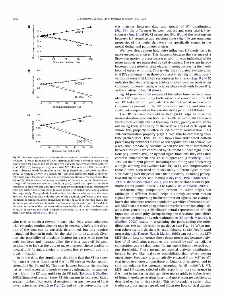
Recordings from MT and MST neurons with random dot motionpresented within their receptive fields revealed roughly linear rela-tionships with positive and negative slopes between responsemagnitude and coherence of motion in the preferred and nulldirections, respectively (Britten, Shadlen, Newsome, & Movshon,1993; Celebrini & Newsome, 1994); see Fig. 11.
3.2. Data explanations
This section explains the data properties that have just beensummarized. Section 2 discusses how the random dot motion stim-ulus causes local directional ambiguity, similar in many respects tothe aperture problem, in the short-range filter stage (V1), and howrecurrent processing in the MT–MST circuit allows the locationswith aperture ambiguities to be captured by FT signals. The mainnew explanatory concept in analyzing the current dataset is that,in the dots task, the effectiveness of this motion capture processis limited by the coherence of the moving dots, and also by theviewing duration. This effectiveness is reflected in a bigger contrastor difference in activity among MT/MST directional cell popula-tions (Fig. 11). This section explains how better performance andfaster reaction time may proportionally be derived from this dy-namic difference. The time course of the activities in model MT
and MST are consistent with those recorded in MT (Britten et al.,1993). One interesting point in Fig. 11 from both data and simula-tions is that the motion-sensitive neurons are active well above thebaseline for a 0% coherence stimulus. This can be explained by not-ing that, if there is no stimulus-induced directional bias, as is thecase at 0% coherence, then random local groupings are formedequally in all directions.
Although MT and MST provide the trial-to-trial neural basis ofdirectional ambiguity on which decisions are made, they exhibitlow choice probabilities (MT: Britten, Newsome, Shadlen, Celebrini,& Movshon, 1996; MST: Celebrini & Newsome, 1994); that is, they‘‘covary only weakly with what the animal decides” (p. 1930 inShadlen & Newsome, 2001) especially at weaker coherences. Whenmonkeys are trained to report the perceived direction through asaccadic eye movement, the recorded dynamics of appropriateLIP cells correlate strongly with decision-making behavior. It ison most error trials that MT/MST (‘‘sensory”) and LIP (‘‘decision”)cells differ in their winning direction. The current consensus inneuroscience is that some sort of a noisy accumulation of sensorysignals is the basic mechanism underlying perceptual decision-making in the brain (Smith & Ratcliff, 2004; see Section 4.3 formore references).
In our model, LIP is modeled as a recurrent competitive field inwhich individual cells are selective for motion directions of fovealstimuli presented outside their response fields. Distinct targets that

0 400 800 -800 -400 020
30
40
50
60
70
Act
ivit
y
Time (ms)
0 400 800 -800 -400 020
30
40
50
60
70
Act
ivit
y
Time (ms)
Fig. 8. Temporal dynamics of LIP responses during error trials in the RT task (Roitman & Shadlen, 2002) for two low coherence levels. Same conventions as in Fig. 5a arefollowed. (a) Average responses from 54 LIP neurons on correct and error trials during the RT task for 3.2% coherence. (b) Model simulations replicate LIP cell recordings onerror trials of the RT task for 3.2% coherence. (c) Average responses from the same population of LIP neurons on correct and error trials during the RT task for 6.4% coherence.(d) Model simulations again capture the data. In (a–d), the colored curves represent correct trials, and the gray curves represent error trials. Solid and dashed curvescorrespond to input stimuli whose motion is towards or away from the right target (Tin)/receptive field, respectively. LIP responses on error trials show that LIP reflects boththe choice the monkey makes, and also the true direction and strength of the dots. Gray curves in the left portion of the plots show that the rates of buildup and decline inaverage LIP activity are relatively lower on error trials. Also, note that the median RT is relatively more on the error trials. [Data in (a,c) is reprinted with permission fromRoitman and Shadlen (2002).]
S. Grossberg, P.K. Pilly / Vision Research 48 (2008) 1345–1373 1355
are visible at a specific eccentricity around the foveal locations,where the dots are displayed, guide the possible alternatives of mo-tion direction the monkey has to choose from. Each LIP cell popula-tion receives convergent excitatory directional inputs from spatiallydistributed cells in foveal MST. This distributed activation providesevidence for the perceptual decision that the global motion is in thedirection from the fovea towards its response field. Operant condi-tioning from foveal MST neurons to these non-foveal LIP neurons isassumed to strengthen the corresponding fovea-to-response fieldconnections. This learning process is not simulated here.
In the model, a choice target creates an excitatory input whosemagnitude is enough for the cells to achieve above-baseline activ-ity before the dots turn on (see Fig. 5 and Appendix Eq. (31)). Whileeach LIP cell gets excited, it is also inhibited by other active LIPcells in the recurrent competitive field. Since a higher percentcoherence in a particular direction, on average, causes faster andmore widespread captured motion signals in MST cells, it alsocauses in LIP cells faster activation via the recurrent on-centerand faster inhibition via the recurrent off-surround for the pre-ferred and non-preferred LIP cells, respectively (Fig. 5).
The model’s LIP-BG loop (Figs. 1 and 4) gates the release ofchoice saccades during both the FD and RT tasks. It is well knownthat such a BG gate controls the release of saccades in vivo; e.g.,Hikosaka and Wurtz (1983, 1989). In the RT task, a decision ismade after either directional LIP activation exceeds a threshold.In particular, stronger motion strength results in faster rise ofactivity for one of the LIP cells to the threshold, causing faster deci-sions, and thereby faster reaction times (Fig. 6c and d). In the FDtask, monkeys are trained to wait to move until the fixation point
is extinguished. In the model, fixation point extinction triggers aGO signal. Thus, for a saccade to be initiated from the fixation pointto the chosen target in either task, the basal ganglia need to firstopen the gate that releases the final decision stage in the targetLIP cell population. This is computationally achieved in the modelby switching the gain of self-excitation of the selected LIP cell to ahigher value. Strong recurrent self-excitation then gets activatedwhich manifests as steep pre-saccadic enhancement, or burst, inLIP firing just before the eyes move. In the model, this gainswitches to a high enough value such that the recurrent signal out-weighs any differential sensory excitation. This property is whatmakes the LIP cell firing for correct Tin choices independent of per-cent coherence in the post-threshold-crossing (RT task, Fig. 5a andb) or post-GO signal (FD task, Fig. 5c–f) stage. This is when LIPswitches, as it were, from the sensory driven mode to the motordecision mode. For correct Tout choices, coherence plays a role evenin the final stages of LIP firing in the RT task because the model BGdo not similarly increase the gain of recurrent inhibition from theselected cell (Fig. 5a and b).
This simple BG mechanism is consistent with detailed models ofhow basal ganglia gates may be dynamically controlled when mon-keys learn to do a range of saccadic eye movement tasks (Brownet al., 2004). The LIP burst response is transformed into the execu-tion of the appropriate saccadic eye movement further down-stream in the brain. Several modeling articles about saccadic andsmooth pursuit eye movements detail these subsequent eye move-ment stages (Gancarz & Grossberg, 1998, 1999; Grossberg, Sriha-sam, & Bullock, submitted for publication; Srihasam, Bullock, &Grossberg, 2008).
0 0.5 1 0
10
20
30
40
50
Time (s)
0 0.5 1 -0.5 0
10
20
30
40
50
Time (s)
0 0.5 1 -0.5 0
10
20
30
40
50
Time (s)
0 0.5 1 -0.5 0
10
20
30
40
50
Time (s)
Mea
n re
spon
se
Mea
n re
spon
se
fe
g h
-0.50 00.5 1 —0.5Time (s)
1.5
0 00.5 1 —0.5Time (s)
1.5
0 00.5 1 —0.5Time (s)
1.5
0 00.5 1 —0.5Time (s)
1.5
Mea
n re
spon
seM
ean
resp
onse
Mea
n re
spon
se
10
20
30
40
50
10
20
30
40
50
10
20
30
40
50
10
20
30
40
50
(spi
kes/
s)M
ean
resp
onse
(spi
kes/
s)M
ean
resp
onse
(spi
kes/
s)M
ean
resp
onse
(spi
kes/
s)
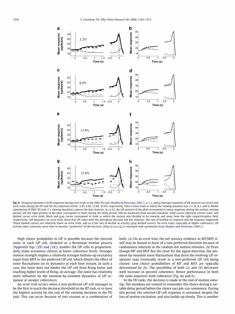
Fig. 9. Temporal dynamics of LIP responses during error trials in the 2001 FD task (Shadlen & Newsome, 2001). (a, c, e, and g) Average responses of LIP neurons on correct anderror trials during the FD task for the coherence levels: 3.2%, 6.4%, 12.8%, 25.6%, respectively. Data is from trials in which the viewing duration was 2 s. (b, d, f, and h) Modelsimulations of 2001 FD task (1 s viewing duration) capture the data features. In (a–h), the left portion of the plots correspond to mean responses during the motion viewingperiod, and the right portion of the plots correspond to those during the delay period, 500 ms backward from saccade initiation. Solid curves represent correct trials, anddashed curves error trials. Black and gray curves correspond to trials in which the motion was decided to be towards and away from the right target/receptive field,respectively. Cell dynamics on error trials show that LIP codes both the perceptual decision and the stimulus. The rate of buildup in response and the response magnitude(black dashed curves) are relatively lower on error trials, and so is the rate of decline in activity (gray dashed curves). On error trials, especially at higher coherences, LIPactivity takes relatively more time to become ‘‘predictive” of the decision. [Data in (a,c,e,g) is reprinted with permission from Shadlen and Newsome (2001).]
1356 S. Grossberg, P.K. Pilly / Vision Research 48 (2008) 1345–1373
High choice probability in LIP is possible because the internalnoise in each LIP cell, modeled as a Brownian motion process(Appendix Eqs. (29) and (34)), enables the LIP cells to proportion-ately make erroneous choices at lower coherence levels. Strongermotion strength implies a relatively stronger bottom-up excitatoryinput from MST to the preferred LIP cell, which dilutes the effect ofnoise fluctuations on its dynamics at each time instant. In such acase, the noise does not hinder the LIP cell from firing faster andreaching higher levels of firing, on average. The noise has relativelymore influence on the moment-by-moment dynamics of LIP re-sponse at weaker coherences.
An error trial occurs when a non-preferred LIP cell manages tobe the first to reach the decision threshold in the RT task, or to havethe highest activity by the end of the viewing duration in the FDtask. This can occur because of two reasons or a combination of
both: (a) On an error trial, the net sensory evidence in MT/MST it-self may be biased in favor of a non-preferred direction because ofrandomness inherent in the random dot motion stimulus. (b) Eventhough MT and MST fire the most for the signal direction, the mo-ment-by-moment noise fluctuations that drive the evolving LIP re-sponses may eventually result in a non-preferred LIP cell beingchosen. Low choice probabilities of MT and MST are typicallydetermined by (b). The possibility of both (a) and (b) decreaseswith increase in percent coherence. Hence performance in boththe tasks improves with coherence (Fig. 6a and b).
In the FD tasks, the decision is made at the end of motion view-ing. The monkeys are trained to remember the choice during a var-iable delay period before the choice saccade can commence. Duringthis period, the selected LIP cell response is sustained, despite theloss of motion excitation, and also builds up slowly. This is another

0 200 400 600 800 100020
25
30
35
40
45
50
55
60
65
70
75
Time (ms)
Act
ivity
0 % 3.2 % 6.4% 12.8 % 25.6 % 51.2 %
0
20
40
60
80
100Sl
ope
of a
ctiv
ity0 10 20 30 40 50
400
600
800
1,000
Motion strength (% coherence)
Med
ian
RT
(ms)
c
s l s l s l s l s l s l
short RTlong RT
short RT grouplong RT group
Fig. 10. Relationship between LIP response and reaction time. At each non-zero coherence, correct trials for the right target (Tin) were sorted into two groups: short RT andlong RT, based on whether the RT is smaller or larger than the median RT. For 0% coherence, trials resulting in Tin choices were considered. (a) Average LIP responses for bothgroups at 6.4% coherence, which are linear fit from 200 ms after motion onset to the median RT of the group, while excluding any activity 100 ms backwards from saccadeinitiation. (b) Model simulation reflects this relationship. The solid curve corresponds to short RT group, and the dashed curve to long RT group. (c) The histogram shows foreach coherence level and group the slope of the linear fit to the average LIP response starting at 200 ms from motion onset, ending at the median RT of the group, andexcluding any spikes within 100 ms before the eyes move. The inset shows at each coherence the median RT for both groups formed from trials of correct Tin choices. (d)Model simulations reproduce these data trends. Dark bars correspond to short RT group, and light bars to long RT group. In (c) and (d), the error bars represent 95% confidenceintervals (CI). [Data in (a,c) is reprinted with permission from Roitman and Shadlen (2002).]
S. Grossberg, P.K. Pilly / Vision Research 48 (2008) 1345–1373 1357
difference with sensory neurons. In the model, the gain of recur-rent excitation of the winning LIP cell switches to a value whichis just high enough to not only compensate for the input from mo-tion areas getting shut off, but also to help its activity to growslowly during the delay period for all motion strengths. The recur-rent self-excitatory interactions within the LIP recurrent competi-tive field thus enable persistent activity for the chosen LIP cell afterthe motion offset. This gain increase hypothesis is consistent withdata showing that an intention to saccade to a particular locationresults in the deployment of some attention to that location (Bisley& Goldberg, 2003). Similar anticipatory activity is seen in superiorcolliculus (SC) buildup neurons in delayed saccade tasks (Gross-berg, Boardman, et al., 1997; Grossberg, Roberts, Aguilar, & Bullock,1997; Munoz & Wurtz, 1995a, 1995b). The fact that the LIP re-sponses in the FD task have a slower rate of growth and a tendencyto saturate when compared to the RT task (Fig. 5) is explained inthe model by using a slightly higher passive decay rate parameterfor the FD task. This parameter change may reflect a task-sensitivechange in the monkey’s LIP responsiveness given the difference inthe two experimental conditions (see p. 1930 in Shadlen & New-some, 2001). The tendency of LIP responses to saturate in the FDtask may, in turn, explain the tendency of performance as a func-
tion of viewing duration to saturate, especially at higher motionstrengths (see Fig. 7).
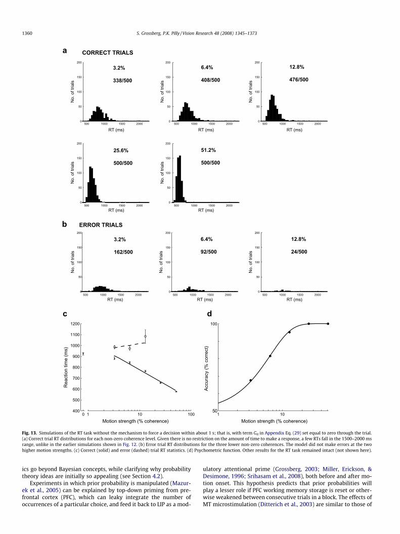
A ‘‘forced choice” is made in the RT task in the manner noted inSection 2; namely, if no choice is made within a random time be-tween 1000 and 1100 ms, then a volitional top-down signal is acti-vated at the LIP cell with the most activity (see term Gd inAppendix Eq. (29)). Fig. 12 shows the model’s RT distributions withthis top-down signal at work. The fraction of simulation trials inwhich a choice needs to be forced decreases with coherence (seeFig. 12d). Fig. 13 shows that the model also works without thistop-down mechanism, but allows for some longer RTs to occur inthe 1500–2000 ms range.
Our proposed mechanism underlying ‘‘forced choices” is com-patible with a different mechanism for the same purpose describedin Ditterich (2006b), in which the gain of MT signals into LIP cellsmonotonically increases with time, and with physiological data re-cently reported by Churchland, Kiani, and Shadlen (2007) of a stim-ulus-independent time-varying signal, which increases with timein each LIP population.
The basic idea behind these mechanisms is to trigger a decisiondespite only a partial resolution among LIP cells as time passes.Ditterich (2006b) argued that this may be important for a monkey
0 10 20 30 40 50 60
0.1
0.2
0.3
0.4
Stimulus correlation (%)
Mea
n re
spon
se
0.0211
0.0839
0 10 20 30 40 50 60
0.05
0.15
0.25
0.35
0.45
Stimulus correlation (%)
Mea
n re
spon
se
0.022
0.0517
Fig. 11. Average responses in motion-sensitive areas as a function of stimulus co-rrelation. (a) Mean responses of an MT neuron at different coherence levels acrossseveral trials for motion in both its preferred and anti-preferred directions (Brittenet al., 1993). (b) Average activity in a model MT cell pool across 500 trials at diff-erent coherence levels for motion in both its preferred and anti-preferred direc-tions. (c) Average activity in a model MST cell pool across 500 trials at differentcoherence levels for motion in both its preferred and anti-preferred directions. Thus(b) and (c) demonstrate the analog sensitivity of the model to the direction andstrength of random dot motion stimuli. In (a–c), closed and open circles showresponses to preferred and anti-preferred random dot motion stimuli, respectively.Solid and dashed lines correspond to least-squares estimated linear and quadraticfits, respectively. The quadratic function describes the data better than the linearfunction. For each quadratic fit, the ratio of the quadratic coefficient to the linearcoefficient is computed, and is shown near the fit. The value of this ratio gives a feelfor the degree of non-linearity in the function relating the coherence of the dots tothe mean response of the motion-sensitive area. In (b) and (c), the standard errorsof mean (SEM) were too small to report in the plots. [Data in (a) is reprinted withpermission from Britten et al. (1993).]
1358 S. Grossberg, P.K. Pilly / Vision Research 48 (2008) 1345–1373
who tries to obtain a reward in each trial. On a weak coherencetrial, extended motion viewing may be necessary before the direc-tion of the dots can be correctly determined, but this requiresmaintained fixation in order for the trial not to be aborted. Giventhat the possibility of breaking fixation increases with time forboth monkeys and humans alike, there is a trade-off betweencontinuing to look at the dots to make a correct choice leading toreward, and forcing a choice to prevent loss of reward due to abreak in fixation.
As in the data, the simulations also show that the RT task per-formance is better than that of the 1 s FD task at weaker motionstrengths (Fig. 6a and b). This may happen because the monkeyhas as much access as it needs to sensory information in ambigu-ous trials in the RT task, unlike in the FD task (Roitman & Shadlen,2002). Simulated reaction time (RT) histograms in fact reveal that agreater number of correct trial reaction times are in excess of 1 s atlower coherence levels (see Fig. 12a and c). It is noteworthy that
the matches between data and model of RT distributions(Fig. 12), the differences between correct and error trial LIP re-sponses (Figs. 8 and 9), RT properties (Fig. 6), and the relationshipbetween LIP response and reaction time (Fig. 10) are emergentproperties of the model that were not specifically sought in themodel design and parameter choices.
We have already seen how noise influences LIP model cells tomake erroneous choices. This happens because the variance of aBrownian motion process increases with time as individual whitenoise samples are integrated by cell dynamics. The system herebybecomes more noisy as time elapses, thereby increasing the likeli-hood of errors with time. This is why the simulated average errortrial RTs are longer than those of correct trials (Fig. 6). Also, obser-vations of error trial LIP cell responses in both tasks (Figs. 8 and 9)indicates the rate of change in activity is lower on error trials whencompared to correct trials, which correlates well with longer RTs,as the analysis in Fig. 10 shows.
Fig. 14 provides some samples of the entire time course of sim-ulated LIP responses during both correct and error trials in the FDand RT tasks. Note in particular the distinct visual and saccadiccomponents present in the LIP response dynamics, and also thesustained component in the variable delay period of FD tasks.
The LIP recurrent competitive field (RCF) helps to solve thenoise-saturation problem because its cells self-normalize the net-work’s total activity, even if their inputs vary greatly in size, with-out losing their sensitivity to the relative sizes of each input. Invision, this property is often called contrast normalization. Thisself-normalization property plays a role akin to computing real-time probabilities. Thus, an RCF shows how distributed patternprocessing by networks of cells, or cell populations, can behave likea real-time probability calculus. When the recurrent interactionsbetween the cells are controlled by faster-than-linear signal func-tions (e.g., power laws), or sigmoid signal functions, they can causecontrast enhancement and noise suppression (Grossberg, 1973,1988) of their input pattern, including the limiting case of selectinga single winning cell (winner-take-all). RCFs, and simplificationsthereof, have been used to model many different types of deci-sion-making over the years since their discovery, including percep-tual and cognitive decision-making (Chey et al., 1997; Francis et al.,1994; Usher & McClelland, 2001) and reach decisions in dorsal pre-motor cortex (Model: Cisek, 2006; Data: Cisek & Kalaska, 2005).
Self-normalizing competition, present in other stages too(although in different forms), helps to amplify coherent motionsignals while suppressing incoherent motion signals. For example,lower dot coherence renders population activities of neurons in MTand MST that are tuned to opponent directions more indistinguish-able, thus generating a distributed neural representation of highinput motion ambiguity. Strengthening one directional pool eitherby bottom-up input or by microstimulation (Ditterich, Mazurek, &Shadlen, 2003) results in weakening the pools coding the otherdirections, the null direction in particular (see Fig. 11). When mo-tion coherence is high, there is less ambiguity, so fast feedforwardprocessing (cf., Thorpe, Fize, & Marlot, 1996) can occur in the MT/MST circuit. Low coherence slows down processing because activ-ities of all conflicting groupings are reduced by self-normalizingcompetition, and it takes longer for any one of them to exceed out-put thresholds. These normalized spatial activity distributionshereby behave like real-time probabilities that reflect systemuncertainty. Feedback is automatically engaged from MST to MTthat helps to choose among these ambiguous alternatives, and tocontrast enhance the strongest grouping. At all model V1, MT,MST, and LIP stages, selected cells respond to more coherence inthe input by increasing their activities more rapidly to higher levelsof firing, thereby generating faster and more accurate decisions asdescribed earlier in this section. This self-organizing system thustrades accuracy against speed, and illustrates how cortical dynam-

500 1000 1500 20000
50
100
150
200
RT (ms)
No.
of t
rials
500 1000 1500 20000
50
100
150
200
RT (ms)
No.
of t
rials
500 1000 1500 20000
50
100
150
200
RT (ms)
No.
of t
rials
500 1000 1500 20000
50
100
150
200
RT (ms)
No.
of t
rials
500 1000 1500 20000
50
100
150
200
RT (ms)
No.
of t
rials
500 1000 1500 20000
50
100
150
200
RT (ms)
No.
of t
rials
500 1000 1500 20000
50
100
150
200
RT (ms)
No.
of t
rials
500 1000 1500 20000
50
100
150
200
RT (ms)
No.
of t
rials
CORRECT TRIALS
ERROR TRIALS
3.2%
324/500
6.4%
412/500
25.6%
500/500
51.2%
500/500
3.2%
176/500
6.4%
86/500
12.8%
475/500
12.8%
25/500
1 10 1000
5
10
15
20
25
30
35
Motion strength (% coherence)
% o
f cor
rect
tria
ls w
ith R
T >
1s
0 1 10 1000
2
4
6
8
10
12
% o
f for
ced
trial
s
Motion strength (% coherence)
correcterror
0
a
b
c d
Fig. 12. Reaction time histograms from simulations of the RT task. In (a), RT statistics from the correct trials are shown. We can observe that as the coherence increases, the RThistogram becomes narrower and shifts to the left. Also, as the coherence decreases, quite a number of trials have RTs in excess of 1000 ms. This may explain why RT taskaccuracy is slightly better than that of 1s FD task at weaker coherence levels. In (b), RT histograms from the error trials are shown. The model monkey does not make anyerrors at stronger coherences: 25.6% and 51.2%. Note the fraction of trials in each panel for the corresponding condition. The bin-width used in generating the histograms is50 ms. The RT distribution data from Roitman and Shadlen (2002) experiments is available in Ditterich (2006a). Panel (c) plots the proportion of correct trials with reactiontime greater than 1000 ms in the simulated RT task at each motion strength. (d) Forced choice task design requires the model to make a choice in each RT task trial howeverambiguous the stimulus is. Sometimes, at low coherences in particular, increased viewing duration does not sufficiently clarify the direction of the dots. In such cases, themodel is forced to make a choice via term Gd in Appendix Eq. (29). In this plot, open circles indicate the proportion of trials (out of 500), when a forced choice was invoked, as afunction of motion strength. This fraction falls off linearly with respect to log10 scale of percent coherence. Open diamonds and squares refer to correct and error decisions,respectively. The forced choices turn out to be correct at slightly better than chance, implying they are not ‘‘pure” guesses.
S. Grossberg, P.K. Pilly / Vision Research 48 (2008) 1345–1373 1359
500 1000 1500 20000
50
100
150
200
RT (ms)
No.
of t
rials
500 1000 1500 20000
50
100
150
200
RT (ms)
No.
of t
rials
500 1000 1500 20000
50
100
150
200
RT (ms)
No.
of t
rials
500 1000 1500 20000
50
100
150
200
RT (ms)
No.
of t
rials
500 1000 1500 20000
50
100
150
200
RT (ms)
No.
of t
rials
500 1000 1500 20000
50
100
150
200
RT (ms)
No.
of t
rials
500 1000 1500 20000
50
100
150
200
RT (ms)
No.
of t
rials
500 1000 1500 20000
50
100
150
200
RT (ms)
No.
of t
rials
CORRECT TRIALS
ERROR TRIALS
3.2%
338/500
6.4%
408/500
25.6%
500/500
51.2%
500/500
3.2%
162/500
6.4%
92/500
12.8%
476/500
12.8%
24/500
c d
0 1 10 100400
500
600
700
800
900
1000
1100
1200
Motion strength (% coherence)
Rea
ctio
n tim
e (m
s)
1 1050
100
Motion strength (% coherence)
Accu
racy
(% c
orre
ct)
a
b
Fig. 13. Simulations of the RT task without the mechanism to force a decision within about 1 s; that is, with term Gd in Appendix Eq. (29) set equal to zero through the trial.(a) Correct trial RT distributions for each non-zero coherence level. Given there is no restriction on the amount of time to make a response, a few RTs fall in the 1500–2000 msrange, unlike in the earlier simulations shown in Fig. 12. (b) Error trial RT distributions for the three lower non-zero coherences. The model did not make errors at the twohigher motion strengths. (c) Correct (solid) and error (dashed) trial RT statistics. (d) Psychometric function. Other results for the RT task remained intact (not shown here).
1360 S. Grossberg, P.K. Pilly / Vision Research 48 (2008) 1345–1373
ics go beyond Bayesian concepts, while clarifying why probabilitytheory ideas are initially so appealing (see Section 4.2).
Experiments in which prior probability is manipulated (Mazur-ek et al., 2005) can be explained by top-down priming from pre-frontal cortex (PFC), which can leaky integrate the number ofoccurrences of a particular choice, and feed it back to LIP as a mod-
ulatory attentional prime (Grossberg, 2003; Miller, Erickson, &Desimone, 1996; Srihasam et al., 2008), both before and after mo-tion onset. This hypothesis predicts that prior probabilities willplay a lesser role if PFC working memory storage is reset or other-wise weakened between consecutive trials in a block. The effects ofMT microstimulation (Ditterich et al., 2003) are similar to those of
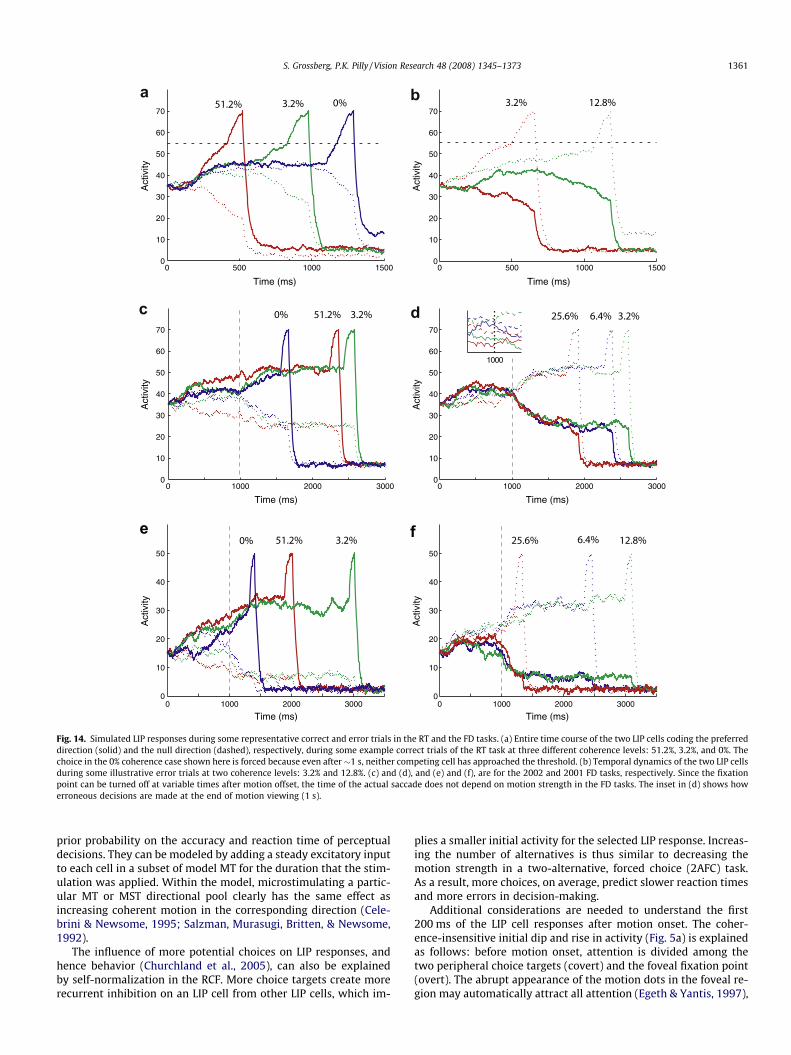
0 500 1000 15000
10
20
30
40
50
60
70
Time (ms)
Act
ivity
0 500 1000 15000
10
20
30
40
50
60
70
Time (ms)
Act
ivity
51.2% 3.2% 0% 3.2% 12.8%
0 1000 2000 30000
10
20
30
40
50
60
70
Act
ivity
0 1000 2000 30000
10
20
30
40
50
60
70
Act
ivity
1000
0% 51.2% 3.2% 25.6% 6.4% 3.2%
0 1000 2000 30000
10
20
30
40
50
Act
ivity
0 1000 2000 30000
10
20
30
40
50
Act
ivity
0% 51.2% 3.2% 25.6% 6.4% 12.8%e f
Time (ms)Time (ms)
Time (ms) Time (ms)
Fig. 14. Simulated LIP responses during some representative correct and error trials in the RT and the FD tasks. (a) Entire time course of the two LIP cells coding the preferreddirection (solid) and the null direction (dashed), respectively, during some example correct trials of the RT task at three different coherence levels: 51.2%, 3.2%, and 0%. Thechoice in the 0% coherence case shown here is forced because even after �1 s, neither competing cell has approached the threshold. (b) Temporal dynamics of the two LIP cellsduring some illustrative error trials at two coherence levels: 3.2% and 12.8%. (c) and (d), and (e) and (f), are for the 2002 and 2001 FD tasks, respectively. Since the fixationpoint can be turned off at variable times after motion offset, the time of the actual saccade does not depend on motion strength in the FD tasks. The inset in (d) shows howerroneous decisions are made at the end of motion viewing (1 s).
S. Grossberg, P.K. Pilly / Vision Research 48 (2008) 1345–1373 1361
prior probability on the accuracy and reaction time of perceptualdecisions. They can be modeled by adding a steady excitatory inputto each cell in a subset of model MT for the duration that the stim-ulation was applied. Within the model, microstimulating a partic-ular MT or MST directional pool clearly has the same effect asincreasing coherent motion in the corresponding direction (Cele-brini & Newsome, 1995; Salzman, Murasugi, Britten, & Newsome,1992).
The influence of more potential choices on LIP responses, andhence behavior (Churchland et al., 2005), can also be explainedby self-normalization in the RCF. More choice targets create morerecurrent inhibition on an LIP cell from other LIP cells, which im-
plies a smaller initial activity for the selected LIP response. Increas-ing the number of alternatives is thus similar to decreasing themotion strength in a two-alternative, forced choice (2AFC) task.As a result, more choices, on average, predict slower reaction timesand more errors in decision-making.
Additional considerations are needed to understand the first200 ms of the LIP cell responses after motion onset. The coher-ence-insensitive initial dip and rise in activity (Fig. 5a) is explainedas follows: before motion onset, attention is divided among thetwo peripheral choice targets (covert) and the foveal fixation point(overt). The abrupt appearance of the motion dots in the foveal re-gion may automatically attract all attention (Egeth & Yantis, 1997),

1362 S. Grossberg, P.K. Pilly / Vision Research 48 (2008) 1345–1373
thereby rapidly creating a strong foveal transient signal (Bisley,Krishna, & Goldberg, 2004) that inhibits both peripheral LIP popu-lations. The foveal transient is independent of the strength of themoving dots. The coherence-independent rise in activity resultsfrom the offset of the initial burst, and the time when LIP activitiesstart fanning-out is when the discriminative motion signals startreaching the LIP choice network. Such lateral inhibition is also con-sistent with recent experimental data and modeling of transientpauses in SC neuronal firing induced in part by shape-changingcues occurring in a region well outside the movement field (Li,Kim, & Basso, 2006). Unlike in the RT task, the interval betweenthe onset of choice targets and that of dots is fixed in the FD task(see p. 9476 in Roitman & Shadlen, 2002), thus effectively eliminat-ing the ‘surprise’ element. The lack of transient pause in LIP firingduring the FD task (Fig. 5c and e) may be a result of this difference.
4. Discussion
4.1. Noise in perceptual decision-making
Cellular noise in LIP influences temporal dynamics and thus thevariability in the accuracy and reaction time of perceptual deci-sions that LIP controls. Model simulations to this point are deter-ministic until the MST stage. In this form, the modelapproximates all internal neuronal noise from Retina to LIP bynoise that drives just the LIP output stage. Trial-to-trial variabilityin the model until MST is elicited only by the randomness inherentin the random dot motion stimuli. However, both MT and MSThave been shown to exhibit response variance even if the same se-quence of random dots is input again and again (Britten et al.,1993; Celebrini & Newsome, 1994).
The above simulations support the hypothesis that noise in LIP,plus the randomness in the stimulus itself, which generates ran-dom cell responses throughout the motion processing stages, issufficient to quantitatively simulate key data properties. In orderto test this directly, we also ran our simulations introducing similarnoise processes in both MT and MST (see Appendix Eqs. (23) and(28)), in addition to the noise in LIP. We tried two different stan-dard deviations (r0) for the internal noise in MT and MST: onecomparable to that used in LIP, and the other five times greater.In both cases, all our results remained qualitatively the same (seeillustrative Fig. 15). For the higher MT and MST noise condition,the psychometric function seems to shift slightly to the right, asone would expect by virtue of more overall noise in the system(threshold ratio aRT;r0¼0:1=aRT;r0¼0:5 ¼ 0:893 < 1; see AppendixA.3.7 for how threshold a is defined). Our data explanations still re-main the same. These simulations show that the absence of cellularnoise in the motion processing system is not a rate-limiting factoras long as there is cellular noise in the model’s LIP output stage.
4.2. Bayesian inference in the brain?
The probabilistic nature of decision-making has led to the pro-posal that classical statistical concepts, such as the Bayes rule, mayapply to decision-making in the brain (Gold & Shadlen, 2001, 2007;Knill & Pouget, 2004; Pouget, Dayan, & Zemel, 2003). It is typicallyargued that variability in neuronal responses and the fact that priorknowledge or information influences what we see and how we be-have implies explicit Bayesian inference in the brain. Bayesian andother general statistical concepts formalize aspects of the uncon-scious inference hypothesis of Helmholtz (2000); namely, that vi-sual system works by making inferences about the world basedupon probable interpretations of incomplete or ambiguous data.Kanizsa (1979) and his disciples have, in contrast, described manyvisual percepts that cannot be explained by unconscious inference.
The Helmholtz vs. Kanizsa perspectives exemplify top-down vs.bottom-up approaches to visual perception, as two extremes in acontinuum. The neural model proposed herein characterizes andjoins together both bottom-up and top-down processes to explainchallenging behavioral and brain data.
The Bayes rule, and related statistical concepts, are so generalthat they may be applied to problems in any science. In particular,the Bayes rule follows from writing the probability of any twoevents I and S, namely p(I,S), in two different ways and then divid-ing both sides of this identity by a term on one side of the equa-tion; see Eqs. (1) and (2) below. This generality is part of itsbroad appeal, but is also its weakness in not providing enough con-straints to discover new models of any particular science. In partic-ular, it does not in itself help to discover the brain design principlesand mechanisms that can effectively process ambiguous motionstimuli. The present article proposes how the brain may make per-ceptual decisions in response to motion stimuli by using organiza-tional principles and detailed neuronal mechanisms that gobeyond a general Bayesian formulation, and clarifies why a Bayes-ian approach may initially seem so appealing.
In the Bayesian framework, given a stimulus I which falls on theRetina, the Bayesian model, or ideal observer, asks what percept Sis most likely to have caused it. The basic idea is to find the S thatmaximizes the posterior probability p(S/I) via the Bayes rule:
pðS=IÞ ¼ pðI=SÞpðSÞpðIÞ : ð1Þ
To derive Eq. (1), the probability p(I,S) of the events I and S is writ-ten in two different ways:
pðI; SÞ ¼ pðI=SÞpðSÞ ¼ pðS=IÞpðIÞ; ð2Þ
and then divided by p(I). The specific usage depends on which of Iand S is observable. I could be a spatial input (static image), or aspatio-temporal input (video). S could be either a distributed pat-tern of neuronal firing in some low or mid-level brain region (con-tour, motion, or depth perception, etc.), or a symbolic percept insome high-level brain region (face, house, or object recognition,etc.). Typical psychophysical experiments require subjects to detector discriminate a perceptual feature and/or estimate its strength.The likelihood p(I/S) assigns a probability to each percept S depend-ing on the amount of consistency with the image I, the prior p(S) isthe probability of the scene description S, and p(I) acts as a normal-izing factor (Kersten, Mamassian, & Yuille, 2004; Kersten & Yuille,2003). For example, Bayesian models of speed perception assumea prior that slower speeds are more frequently perceived (Stocker& Simoncelli, 2006; Weiss, Simoncelli, & Adelson, 2002).
Bayesian and other general statistical approaches do not ad-dress how the units of stimulus I and percept S are generated bythe brain, such as illusory contours, which are emergent propertiesnot explicit in the luminance levels of an inducing image. Bayesianmodels also do not explain percepts of environments whose statis-tics change through time, where there is no obvious likelihood p(I/S), or novel rare percepts, where there is no obvious prior p(S).Most importantly, it does not explain the brain processes wherebywe perceive.
How might Eq. (1) be applied to motion direction discrimina-tion? Gold and Shadlen (2001) propose that the brain may accu-mulate the logarithm of the posterior ratio (logPR) in a sensory-motor association area such as cortical area LIP. In this situation,the brain has to discriminate between opponent motion directions,say S1 and S2, given the spatio-temporal input I
*
. The posterior ratiois defined as:
PR ¼ pð I*
=S1ÞpðS1Þ
pð I*
=S2ÞpðS2Þ: ð3Þ

0 200 400 600 800 0-200-400-600-80020
30
40
50
60
70
Time (ms)
Activ
ity
1 1 050
100
Motion strength (% coherence)
Accu
racy
(% c
orre
ct)
1 1 0 100400
500
600
700
800
900
1000
Motion strength (% coherence)
Rea
ctio
n tim
e (m
s)
0 200 400 600 800 0-200-400-600-800
Time (ms)
20
30
40
50
60
70
Activ
ity
50
100
Accu
racy
(% c
orre
ct)
1 1 0Motion strength (% coherence)
1 1 0 100Motion strength (% coherence)
400
500
600
700
800
900
1000
Rea
ctio
n tim
e (m
s)
0 0
b e
c f
Fig. 15. Simulations of the RT task with noise in both MT and MST. See Appendix Eqs. (23) and (28). The level of noise was about the same as that used in LIP (see Appendix).(a) Correct trial LIP cell dynamics for all motion strengths in either motion direction. Same conventions as in Fig. 5a are used. (b) Correct (solid) and error (dashed) trial RTs atvarious coherences. (c) Psychometric function. Noise in MT and MST also did not affect other RT task results (not shown here). (d–f) Simulations of the RT task with morenoise in MT and MST. The level of noise was five times greater than that used in the simulations shown in (a)–(c).
S. Grossberg, P.K. Pilly / Vision Research 48 (2008) 1345–1373 1363
Taking a logarithm on both sides yields a difference of two logs:
log PR ¼ log pð I*
=S1ÞpðS1Þ � log pð I*
=S2ÞpðS2Þ: ð4Þ
When both directions are equally probable, p(S1) = p(S2), logPR re-duces to log-likelihood ratio (logLR):
log LR ¼ log pð I*
=S1Þ � log pð I*
=S2Þ: ð5Þ
Gold and Shadlen (2001, 2007) suggest that the difference in activ-ities of two populations in middle temporal area (MT) that aretuned to opponent directions approximates a scaled version oflogLR. Motion opponency is known to occur in MT (Albright, Desi-
mone, & Gross, 1984; Heeger, Boynton, Demb, Seidemann, & New-some, 1999; Snowden, Treue, Erickson, & Andersen, 1991), andplays a role in our model as well (Figs. 1 and 4), but its proposedtheoretical equivalence with logLR does not add to our understand-ing of the neuronal dynamics during perceptual decision-making inresponse to a wide variety of perceptual stimuli. In particular, it isnot clear how the concept of logLR extends to multiple-choice tasks,and any log approximation to neuronal activations and firing is bio-logically implausible because the log grows without bound, unlikecellular activations and firing, as its argument increases.
Given these concerns, it is natural to ask if such general statis-tical formulations provide the best currently available approach to

1364 S. Grossberg, P.K. Pilly / Vision Research 48 (2008) 1345–1373
modeling perception and decision-making? As illustrated hereinand in a growing number of other studies, biophysically detailedmodels of visual cortex can quantitatively simulate neurophysio-logically recorded dynamics of identified cells in anatomically sup-ported circuits, and the perceptual and behavioral data that theygenerate as emergent properties. Moreover, these models embodynew design principles, mechanisms, local circuits, and global archi-tectures that are proposed to solve fundamental problems facingthe brain. The present model shows how brain circuits may carryout hypothesis-testing and decision-making in response to bothstatistically changing and novel rare events.
It should also be noted that any filtering operation, such as theshort-range and long-range filters (see Appendix Eqs. (15) and(22)), may be interpreted as a prior (namely, the current neural sig-nal) multiplied by a conditional probability or likelihood (namely,the filter connection strength to the target neurons). Likewise, acontrast-enhancing operation, such as the LIP recurrent on-centeroff-surround network (see Appendix Eq. (29)), that responds tosuch a filter may be viewed as maximizing the posterior. These in-sights have been discussed in the neural modeling literature for along time; e.g., Grossberg (1978). However, as Fig. 1 and the totalset of model equations illustrate, such local processes do not, inthemselves, embody the design principles and computationalintelligence of a behaviorally competent neural system.
In order to contribute to the characterization of how the braincarries out motion processing and decision-making, the presentwork further develops and integrates models that have been grad-ually elaborated to explain and simulate increasingly large databases about motion-based percepts and behaviors through theyears. This emerging motion model, which is often called the 3DFORMOTION model, has simulated a large number of motion per-cepts (see Fig. 16 for two examples). These percepts include aspectsof barberpole illusion; motion capture; spotted barberpole illusion;triple barberpole illusion; occluded translating square illusion; mo-tion transparency; chopsticks illusion; short-range and long-rangeapparent motion, including beta, gamma, reverse-contrast gamma,delta, split, ternus, and reverse-contrast ternus motion; visual iner-tia; Korté’s laws; second-order motion; form-motion interactions,including the line motion illusion, motion induction, and transfor-mational apparent motion; how component angles, contrasts, anddurations influence barberpole and (type 1 and type 2) plaid coher-ence and incoherence; the effects on perceived speed of stimuluscontrast, duration, dot density, orientation, length, and spatial fre-quency; and the effects of parvocellular and magnocellular lateralgeniculate nucleus lesions on motion perception (Baloch & Gross-berg, 1997; Baloch, Grossberg, Mingolla, & Nogueira, 1999; Berzh-anskaya et al., 2007; Chey et al., 1997, Chey, Grossberg, &Mingolla, 1998; Francis & Grossberg, 1996b; Grossberg et al.,2001; Grossberg & Rudd, 1989, 1992). The parameters in this modelare chosen within a robust parameter range to enable all of the pro-cessing stages to contribute their share to the disambiguation of lo-cally ambiguous motion direction.
The fact that the current explanations and simulations of thetemporal dynamics of decision-making in response to probabilisti-cally defined displays of moving dots may be added to this com-pendium of results, without explicitly involving Bayesianconcepts, provides additional evidence that specific brain designsto solve the aperture problem and the noise-saturation problemare indeed at work.
4.3. Stochastic decision models
Various sorts of stochastic reaction time models have long beenused in cognitive psychology to account for both psychometric andchronometric functions of human subjects in a number of percep-tual and cognitive tasks (e.g., Busemeyer & Townsend, 1993; Luce,
1986; Ratcliff, 1978, 1980; Ratcliff, van Zandt, & McKoon, 1999;Ratcliff & Smith, 2004; Smith, 1990, 2000; Smith & Vickers,1988). Most of these models are variants of a diffusion model, ora random-walk model in discrete-time. In the race or accumulatormodel for multiple-choice RT tasks, an accumulator cell yd for eachpossible alternative d gradually integrates its corresponding noisyevidence until one of the cell activities first rises to a decisionthreshold, thereby deciding both the choice and the decision time.The reaction time is computed by adding to the decision time anindependent, random non-decision time to account for sensoryand motor latencies. All diffusion models make assumptionsregarding how perceptual stimuli map into internal sensory repre-sentations, which in turn are converted into decision variables (yd)as follows:
dyd
dt¼ Sd þ r
dWdt
; ð6Þ
where Sd is called the drift rate of the diffusion process for alterna-tive d, which is an increasing function of its internal signal, and thestimulus-independent parameter r scales the standard deviation ofthe Brownian motion process W. The noise term r dW
dt controls choiceand decision time variability. In an FD task, the choice is typicallygoverned by the decision cell with the greater activity at the endof the fixed duration (Ratcliff, 1978).
This simple model can fit the psychometric function, RTs on cor-rect trials, and effects of speed–accuracy trade-off by adjusting thedecision threshold based on priority instructions (Reddi & Carpen-ter, 2000), but needs extensions to tackle relative error trial RTs(Palmer et al., 2005). Some of the variations include dynamic driftrate (Ratcliff, 1980), trial-to-trial variability in drift rate, which cansimulate longer error trial RTs (Ratcliff & Rouder, 1998), and trial-to-trial variability in the starting point of integration, which cansimulate faster error trial RTs in the urgency condition (Ratcliffet al., 1999). Other variants include leaky integration (Smith,2000; Usher & McClelland, 2001), differences between alternativeinternal signals in the sensory read-out stage (Ditterich, 2006a,2006b; Mazurek et al., 2003), and lateral inhibition among accu-mulator cells (Usher & McClelland, 2001).
Neural correlates of decision-making have only recently beeninvestigated in both primates (Glimcher, 2003; Gold & Shadlen,2007; Platt, 2002; Romo & Salinas, 2001; Schall, 2003) and humans(Heekeren, Marrett, Bandettini, & Ungerleider, 2004). Accordingly,general diffusion models have begun to model both behavioral andneurophysiological data in, for example, LIP (Mazurek et al., 2003)and SC (Ratcliff, Cherian, & Segraves, 2003). Studies such as Ratcliffet al. (2003) provide good fits to neurophysiological data frombuildup cells in the deeper layers of the SC during a two-choicedecision task. Although such a diffusion model is more dynamicalthan a general statistical model, it is a formal model that does notembody the brain mechanisms that characterize neural decisionprocesses.
Neural models currently exist that quantitatively simulate thetemporal dynamics of both burst and buildup cells in the SC (Gan-carz & Grossberg, 1999; Grossberg, Roberts, et al., 1997). Unlike thediffusion model, the SC neural model clarifies the different func-tional roles of both cell types, notably how they help to adaptivelyrecode the several types of SC inputs (retinotopic visual inputs,head-centered auditory inputs, and planned prefrontal inputs) intothe same coordinate representation wherein all the inputs cancompetitively choose the next saccadic decision. The currentMODE model attempts to provide a similar functional and mecha-nistic neural understanding of motion-based decision-making.
Four other models (Ditterich, 2006a, 2006b; Mazurek et al.,2003; Wang, 2002) have discussed the Shadlen and Newsome data.We now highlight similarities and differences between our modeland these alternative models.
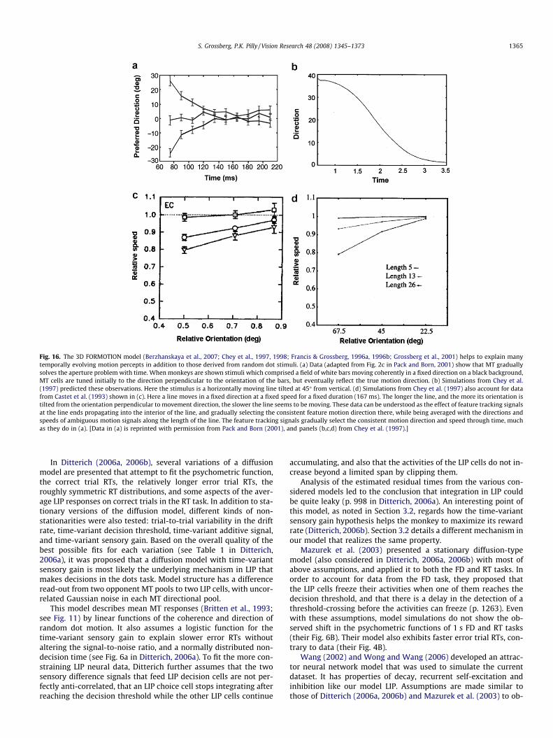
Fig. 16. The 3D FORMOTION model (Berzhanskaya et al., 2007; Chey et al., 1997, 1998; Francis & Grossberg, 1996a, 1996b; Grossberg et al., 2001) helps to explain manytemporally evolving motion percepts in addition to those derived from random dot stimuli. (a) Data (adapted from Fig. 2c in Pack and Born, 2001) show that MT graduallysolves the aperture problem with time. When monkeys are shown stimuli which comprised a field of white bars moving coherently in a fixed direction on a black background,MT cells are tuned initially to the direction perpendicular to the orientation of the bars, but eventually reflect the true motion direction. (b) Simulations from Chey et al.(1997) predicted these observations. Here the stimulus is a horizontally moving line tilted at 45� from vertical. (d) Simulations from Chey et al. (1997) also account for datafrom Castet et al. (1993) shown in (c). Here a line moves in a fixed direction at a fixed speed for a fixed duration (167 ms). The longer the line, and the more its orientation istilted from the orientation perpendicular to movement direction, the slower the line seems to be moving. These data can be understood as the effect of feature tracking signalsat the line ends propagating into the interior of the line, and gradually selecting the consistent feature motion direction there, while being averaged with the directions andspeeds of ambiguous motion signals along the length of the line. The feature tracking signals gradually select the consistent motion direction and speed through time, muchas they do in (a). [Data in (a) is reprinted with permission from Pack and Born (2001), and panels (b,c,d) from Chey et al. (1997).]
S. Grossberg, P.K. Pilly / Vision Research 48 (2008) 1345–1373 1365
In Ditterich (2006a, 2006b), several variations of a diffusionmodel are presented that attempt to fit the psychometric function,the correct trial RTs, the relatively longer error trial RTs, theroughly symmetric RT distributions, and some aspects of the aver-age LIP responses on correct trials in the RT task. In addition to sta-tionary versions of the diffusion model, different kinds of non-stationarities were also tested: trial-to-trial variability in the driftrate, time-variant decision threshold, time-variant additive signal,and time-variant sensory gain. Based on the overall quality of thebest possible fits for each variation (see Table 1 in Ditterich,2006a), it was proposed that a diffusion model with time-variantsensory gain is most likely the underlying mechanism in LIP thatmakes decisions in the dots task. Model structure has a differenceread-out from two opponent MT pools to two LIP cells, with uncor-related Gaussian noise in each MT directional pool.
This model describes mean MT responses (Britten et al., 1993;see Fig. 11) by linear functions of the coherence and direction ofrandom dot motion. It also assumes a logistic function for thetime-variant sensory gain to explain slower error RTs withoutaltering the signal-to-noise ratio, and a normally distributed non-decision time (see Fig. 6a in Ditterich, 2006a). To fit the more con-straining LIP neural data, Ditterich further assumes that the twosensory difference signals that feed LIP decision cells are not per-fectly anti-correlated, that an LIP choice cell stops integrating afterreaching the decision threshold while the other LIP cells continue
accumulating, and also that the activities of the LIP cells do not in-crease beyond a limited span by clipping them.
Analysis of the estimated residual times from the various con-sidered models led to the conclusion that integration in LIP couldbe quite leaky (p. 998 in Ditterich, 2006a). An interesting point ofthis model, as noted in Section 3.2, regards how the time-variantsensory gain hypothesis helps the monkey to maximize its rewardrate (Ditterich, 2006b). Section 3.2 details a different mechanism inour model that realizes the same property.
Mazurek et al. (2003) presented a stationary diffusion-typemodel (also considered in Ditterich, 2006a, 2006b) with most ofabove assumptions, and applied it to both the FD and RT tasks. Inorder to account for data from the FD task, they proposed thatthe LIP cells freeze their activities when one of them reaches thedecision threshold, and that there is a delay in the detection of athreshold-crossing before the activities can freeze (p. 1263). Evenwith these assumptions, model simulations do not show the ob-served shift in the psychometric functions of 1 s FD and RT tasks(their Fig. 6B). Their model also exhibits faster error trial RTs, con-trary to data (their Fig. 4B).
Wang (2002) and Wong and Wang (2006) developed an attrac-tor neural network model that was used to simulate the currentdataset. It has properties of decay, recurrent self-excitation andinhibition like our model LIP. Assumptions are made similar tothose of Ditterich (2006a, 2006b) and Mazurek et al. (2003) to ob-

1366 S. Grossberg, P.K. Pilly / Vision Research 48 (2008) 1345–1373
tain MT responses. Unlike Mazurek et al. (2003), Wang generatespersistent activity in LIP cells in the FD task using strong recurrentexcitation within the same network that integrates noisy evidencein the initial period of the trial. As noted previously, our model LIPRCF employs self-excitation too, but also in the RT task to explainthe steep, coherence-independent motor preparatory activity, andfor quantitative simulations of LIP cell dynamics in the FD taskthrough the entire trial, the delay period in particular (compareour Fig. 5d and f to Fig. 9A in Wong & Wang, 2006).
Both Mazurek et al. (2003) and Wang (2002) employ the samedecision rule in both FD and RT tasks, namely the same decisionthreshold-crossing. In Wang’s FD task simulations, if none of theattractor cells wins (that is, reaches the threshold) within the givenduration, a random choice is made. It is not clear in Mazurek et al.(2003) about what happens if no threshold-crossing occurs withinthe fixed duration.
As we have seen in the RT task, the average LIP responses for Tin
choices, when aligned to saccade onset and grouped by coherencelevel, reveal a firing level, or decision threshold, above whichcoherence does not differentiate the dynamics (see Fig. 5a). Evenif it is assumed that FD task choices are also based on a thresh-old-cross, as in the RT talk, the disparate response ranges duringthe decision formation epoch in the two tasks (compare Fig. 5a(RT task) and 5c (FD task): data from the same monkeys) at leastrule out a common threshold value. As a result, the Mazureket al. (2003) model does not match the recorded LIP response rangeduring motion viewing in the FD task (their Fig. 7C), despite its spe-cialized hypotheses for the FD task. Wang (2002) avoided this issueby emphasizing that model simulations are only qualitative. Incontrast, our model makes FD task choices based on the maximallyactivated LIP cell at the end of the viewing duration (as proposed inGold & Shadlen, 2003, p. 635), and also simulates the task-depen-dent changes in LIP responses.
Our MODE model shares with these alternative models thehypotheses that decisions are made in LIP by accumulating noisymotion signals from MT/MST, and that noise influences the errone-ous choices made by LIP. Our model does not, however, need tomake many of the special hypotheses of the other models becauseit explicitly represents the spatially distributed neural dynamics ofmotion and decision processing in response to the stimuli used inthe experiments.
Leakage and lateral inhibition are modeled in the leaky compet-ing accumulator (LCA) model (Usher & McClelland, 2001) that sim-ulates human behavioral data from other perceptual tasks inboth FD and RT paradigms. Its simulations show how leakage alle-viates the need for trial-to-trial variability in drift rate (Ratcliff,1978; Ratcliff & Rouder, 1998) to explain how improvement in per-formance due to more exposure duration stops at longer durations.Usher and McClelland use a Grossberg Additive Model with thresh-old-linear competitive signals that have been proved capable ofmaking decisions (cf., Grossberg, 1978, 1988). The model alsoincorporates a noise term to simulate stochastic decision data:
dyd
dt¼ �AYd þ kSd � g
XD6¼d
YD þ rdWdt
; and Yd ¼ ½yd�þ: ð7Þ
Usher and McClelland (2001, p. 553) acknowledged these anteced-ents to their use of the Additive Model, and also (p. 555 and 557)that they do not incorporate recurrent excitation in Eq. (7), whichplays an important role of selecting winners in response to inputsthat can vary widely in size (Grossberg, 1973, 1978). Our modelLIP (Appendix Eqs. (29) and (34)) uses a recurrent competitive field,or RCF, also called a Grossberg Shunting Model, that has properties ofautomatic gain control, self-normalization, and self-maintenance ofactivity between maximum and minimum levels, unlike the Addi-tive Model (Grossberg, 1973, 1978, 1988). As noted above, the
Shunting Model embodies these properties in a network with recur-rent excitation and inhibition. They enable our LIP RCF to respondwithout a loss of sensitivity to spatially distributed inputs from abrain region like MST whose cell activations can vary widely innumber and size through time, and can thereby control effectivechoice behavior.
The biggest departure of our model from previous ones is that itdescribes the spatially distributed dynamics of multiple brain areas(Retina/LGN, V1, MT, MST) in the motion pathway leading to LIP,and interactions of the basal ganglia with LIP to make decisions.In particular, we show how principles and mechanisms that haveevolved in the brain to tackle the aperture problem and thenoise-saturation problem may also explain data about the dotstask. Our model also meets the challenge of directly processingthe random dot motion experimental stimuli as real-time inputsat 60 Hz, and its emergent properties fit the widest range of deci-sion-making data in this paradigm of any available model.
Model simulations are consistent with the interpretation ofNewsome, Shadlen, and colleagues regarding the different rolesof ‘‘sensory” MT/MST and ‘‘decision” LIP cells in the motion tasks(see Discussion in Shadlen & Newsome, 2001). In particular, modelMT/MST cells are involved in motion capture and resolve the verid-ical direction of the kinetic dots as much as possible, irrespective ofthe choice made in each trial by LIP cell dynamics. Accordingly, wepropose a lower choice probability in LIP if, for example, the mon-key were to shows its decision using a hand movement (Fig. 7 inNichols & Newsome, 2002), not an eye movement, or if the taskprevents saccade planning during the motion viewing period (Gold& Shadlen, 2003; Horwitz, Batista, & Newsome, 2004b).
The model can also explain how microstimulation to MT andMST influences the accuracy of perceptual decisions (Celebrini &Newsome, 1995; Salzman et al., 1992), how MT microstimulationinfluences correct and error trial RTs (Ditterich et al., 2003), andthe effects of prior probability (Mazurek et al., 2005) and multiplechoices (Churchland et al., 2005). The model also simulates theinfluence of viewing duration on performance at each motionstrength, and thereby the psychometric function (Gold & Shadlen,2003).
In addition, our model goes beyond alternate models by: incor-porating the difference in LIP responsiveness to the two task condi-tions, in particular that the ‘‘gain of the LIP response is greater in theRT version of the task” (p. 9485 in Roitman & Shadlen, 2002); con-sidering the visual contribution to LIP response due to the presenceof the choice target in the receptive field (p. 1931 in Shadlen & New-some, 2001); simulating the entire time course of LIP responsesduring both FD and RT tasks on both correct and error trials forall experimented coherences and directions, in particular the pre-motion onset period activity, the pre-saccadic enhancement (forTin choices) and post-saccadic inhibition in activity (for both tasks),and the variable delay period activity (for FD task); and highlightingthe important role of BG in contextually gating the saccadic re-sponse, depending on whether the task is an FD or an RT type.
4.4. Some model predictions
The MODE model explains and simulates the major data prop-erties derived from the popular random dot motion discriminationexperiments in terms of how the brain solves the aperture problemby using feature tracking signals to provide the best estimates pos-sible of object motion directions. The motion processing stages ofthe model are capable of handling arbitrary motion stimuli. Wepredict that several stimulus manipulations should shift the psy-chometric function to the right, increase reaction times, and haveinfluences on MT, MST, and LIP responses similar to those that oc-cur due to lowering the motion strength. These manipulations in-clude using higher dot density, more interleaved sequences, briefer

S. Grossberg, P.K. Pilly / Vision Research 48 (2008) 1345–1373 1367
signal dots, and more spatial displacement of signal dots betweenframes.
Another prediction regards the lack of coherence-independentinitial transient pause in LIP activity in the FD tasks that can be seenin Fig. 5c and e, unlike in the RT task (see Fig. 5a), due to the predict-ability of motion onset after the choice targets turn on. Self-normal-ization of the recurrent competitive field predicts lower LIP pre-motion onset period activity in multiple-choice experiments thatuse more choice targets (cf., Basso & Wurtz, 1998).
The model hypothesis that a volitionally activated top-downsignal can help to make a ‘‘forced choice” in difficult RT task trialsis a prediction that already has some support from recent data(Churchland et al., 2007). Also testable is the model explanationfor how the average LIP responses in the RT task for correct Tout
choices continue to be influenced by motion strength, even inthe final stages before the saccade is initiated.
4.5. Outstanding issues
All oculomotor areas have been shown to be ‘‘choice-predictive”in the direction discrimination experiments discussed in this arti-cle. This is usually understood by the fact that the monkeys weretrained to indicate their perceptual decision using a saccadic eyemovement, and not some other response. In particular, cells inother saccadic areas (SC, FEF, Area 46), whose response fields con-tain just one choice target, exhibit direction-selective and decision-related activity (Horwitz & Newsome, 2001b; Kim & Shadlen,1999) similar to those in LIP. Given the extensive reciprocal con-nectivity among these areas, it remains to analyze in each particu-lar experimental paradigm which saccade-related area selects thetarget and relays it to other areas. The locus of the ‘‘decision-maker” is of particular interest in ‘‘abstract” versions of the basicdirection discrimination task, which dissociate the decision-mak-ing process from programming of the movement that leads to re-ward (Gold & Shadlen, 2003; Horwitz et al., 2004b). In theseexperiments, the targets are not present during motion viewing,and appear only after motion offset and at unpredictable locations.Hence, a choice target cannot be selected and the saccade vectorcannot be computed until after the kinetic dots shut off, unlike insimpler tasks in which the saccade can be planned while the mo-tion cues are still on. Involvement of the prefrontal cortex is likelyin such memory and rule-based planned movements.
Another issue concerns how the monkey learns the task strategywithin an operant conditioning framework (Born, 2004; Uka &DeAngelis, 2004)? In the experiments simulated herein, monkeyshad to choose between two peripheral choice targets based on mo-tion information extracted from the foveal display. It is likely thatonly those pools of foveal neurons in MT and MST that computeeither right or left motion direction gradually get associated withappropriate populations in several oculomotor structures becauseof extensive training on the task. As a result, LIP cells are able toshow direction selectivity to motion stimuli presented well outsidetheir classical receptive fields (Shadlen & Newsome, 2001). A mon-key whose brain is well-shaped for this particular task may not beable to immediately perform an almost identical task requiring, in-stead, an up vs. down direction discrimination, because the relaylinks of the pertinent sensory representation to the applicablechoice networks, wherever they are present, are not yet learned(Freedman & Assad, 2006). If, moreover, a monkey has been trainedto do both the above tasks, interesting issues of task strategy-switching that can be triggered by contextual cues come to the fore.
This is in contrast to human subjects who can perform any ver-sion of the task, even the abstract ones, just by a mere instruction,probably because of facilitation by language. Explaining the neuralmechanisms whereby language achieves such flexibility is a largetheoretical challenge.
The model hypotheses about how the basal ganglia may gatemovement decisions are highly simplified. A more thorough anal-ysis of how laminar prefrontal cortical circuits interact with the ba-sal ganglia, sensory cortices, and other subcortical structures tolearn and perform movement tasks is provided by the TELOS modelof Brown et al. (2004). Here, after the model incrementally learnedfive different movement tasks that monkeys have been trained toperform, it quantitatively simulated the neurophysiologically re-corded dynamics of seventeen different cell types in these brain re-gions when those tasks were performed. Future modeling workwill incorporate a more complete representation of such prefrontaland basal ganglia interactions with sensory cortices.
Appendix A. Model equations and parameters
A.1. Inputs
Model inputs were random dot motion sequences at varyinglevels of coherence. They were generated in MATLAB 7.1 as de-scribed in the neurophysiological experiments being simulated;see http://cns.bu.edu/~advait/RDMstimuli.html. Three indepen-dent two-dimensional movie sequences were first produced, andthen interleaved to obtain the actual input, which was presentedto the model in real time at the frame rate of 60 Hz. Each framewas a 60 � 60 grid with 100 white dots (intensity = 255) of size1 � 1 on a black background (intensity = 0). The number of dotsper frame may appear to be more than 100 because of visual per-sistence. In the first frame in each of the three sequences, the dotswere randomly placed. For the subsequent frames, a fixed fractionof dots (% coherence) from the immediately previous frame wererandomly chosen, and displaced by 1 pixel in the signal direction(either left or right), and the remaining dots were relocated ran-domly. Thus in every frame, a new fraction of dots was chosen tomove in the signal direction. Varying this fraction hence controlsthe motion strength of the dot display. Given the three framesinterleaving and 60 Hz refresh rate, the effective speed of the signaldots was 20 pixels/s, and there was systematic correlation amongthe temporary signal dots with a phase of three frames. If any sig-nal dot moved out of the grid, then it was wrapped around to ap-pear from the opposite side and thus be within the grid.
The phenomenology of the inputs thus created was confirmedby testing informally with many human subjects. The simulationexperiment comprised 500 trials at each of six coherence levels,which were as follows: 0%, 3.2%, 6.4%, 12.8%, 25.6%, and 51.2%.Zero-percent coherence corresponds to no correct global motiondirection. For all non-zero coherences, the correct direction was al-ways ‘‘Right” for the sake of simplicity. In the monkey experiments,trials were randomly and equally distributed between the ‘‘Left”and the ‘‘Right” directions both to prevent monkeys from develop-ing a bias towards either direction and to study how the non-se-lected target cells would respond (see Section 3). This is not anissue in the simulations because we explicitly model two LIP pop-ulations which prefer the two opponent motion directions (seeAppendix A.3.6). The model was found to work also for the inputframe rate of 75 Hz (Results not included). Note that the modelintegration time-step Dt = 0.001 s is much smaller than 1/60 = 0.0167 s or 1/75 = 0.0133 s (inter-frame duration) so thatinformation embedded in inter-frame transitions is registered.
A.2. Shunting and habituative dynamics
Each cell in the network is modeled using a membrane equation(Grossberg, 1973; Hodgkin & Huxley, 1952), which can be written as:
dVdt¼ a½�bV þ ðc� VÞIex � ðV þ dÞIin�: ð8Þ
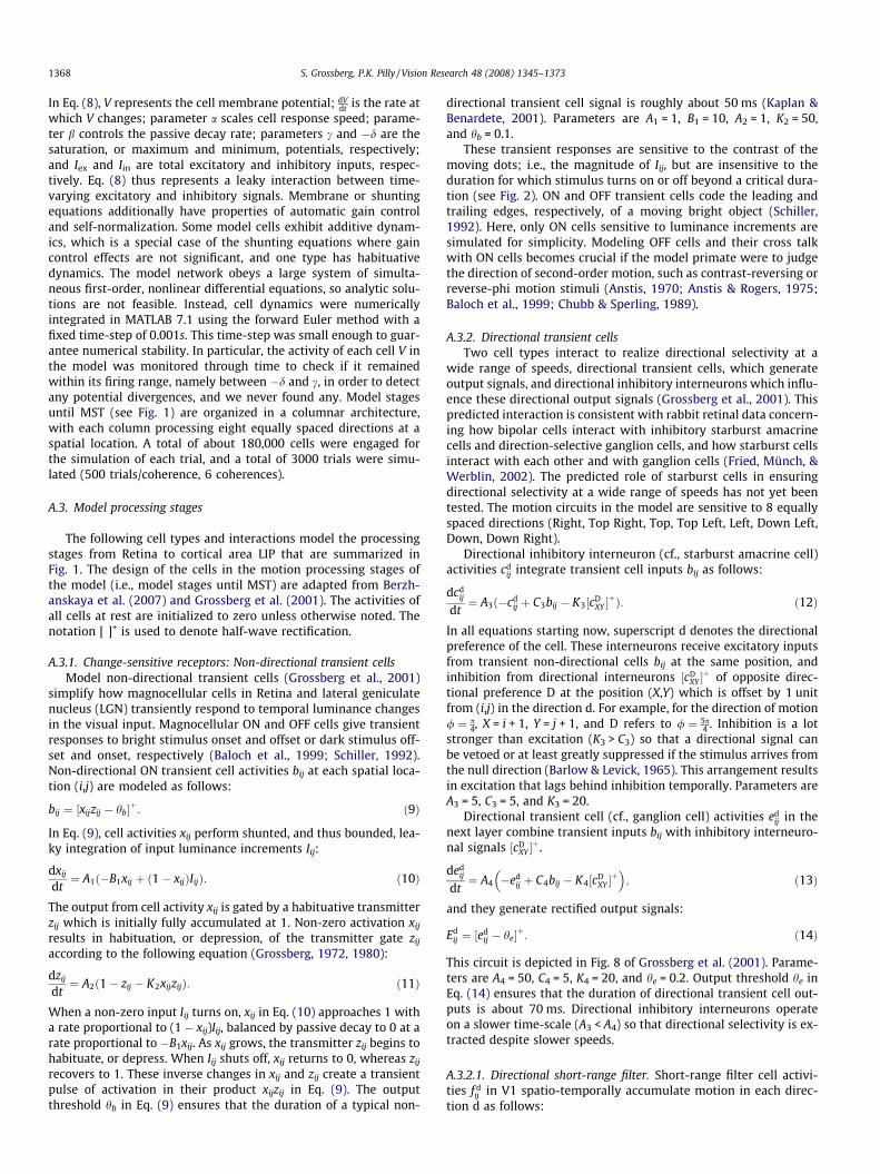
1368 S. Grossberg, P.K. Pilly / Vision Research 48 (2008) 1345–1373
In Eq. (8), V represents the cell membrane potential; dVdt is the rate at
which V changes; parameter a scales cell response speed; parame-ter b controls the passive decay rate; parameters c and �d are thesaturation, or maximum and minimum, potentials, respectively;and Iex and Iin are total excitatory and inhibitory inputs, respec-tively. Eq. (8) thus represents a leaky interaction between time-varying excitatory and inhibitory signals. Membrane or shuntingequations additionally have properties of automatic gain controland self-normalization. Some model cells exhibit additive dynam-ics, which is a special case of the shunting equations where gaincontrol effects are not significant, and one type has habituativedynamics. The model network obeys a large system of simulta-neous first-order, nonlinear differential equations, so analytic solu-tions are not feasible. Instead, cell dynamics were numericallyintegrated in MATLAB 7.1 using the forward Euler method with afixed time-step of 0.001s. This time-step was small enough to guar-antee numerical stability. In particular, the activity of each cell V inthe model was monitored through time to check if it remainedwithin its firing range, namely between �d and c, in order to detectany potential divergences, and we never found any. Model stagesuntil MST (see Fig. 1) are organized in a columnar architecture,with each column processing eight equally spaced directions at aspatial location. A total of about 180,000 cells were engaged forthe simulation of each trial, and a total of 3000 trials were simu-lated (500 trials/coherence, 6 coherences).
A.3. Model processing stages
The following cell types and interactions model the processingstages from Retina to cortical area LIP that are summarized inFig. 1. The design of the cells in the motion processing stages ofthe model (i.e., model stages until MST) are adapted from Berzh-anskaya et al. (2007) and Grossberg et al. (2001). The activities ofall cells at rest are initialized to zero unless otherwise noted. Thenotation [ ]+ is used to denote half-wave rectification.
A.3.1. Change-sensitive receptors: Non-directional transient cellsModel non-directional transient cells (Grossberg et al., 2001)
simplify how magnocellular cells in Retina and lateral geniculatenucleus (LGN) transiently respond to temporal luminance changesin the visual input. Magnocellular ON and OFF cells give transientresponses to bright stimulus onset and offset or dark stimulus off-set and onset, respectively (Baloch et al., 1999; Schiller, 1992).Non-directional ON transient cell activities bij at each spatial loca-tion (i,j) are modeled as follows:
bij ¼ ½xijzij � hb�þ: ð9Þ
In Eq. (9), cell activities xij perform shunted, and thus bounded, lea-ky integration of input luminance increments Iij:
dxij
dt¼ A1ð�B1xij þ ð1� xijÞIijÞ: ð10Þ
The output from cell activity xij is gated by a habituative transmitterzij which is initially fully accumulated at 1. Non-zero activation xij
results in habituation, or depression, of the transmitter gate zij
according to the following equation (Grossberg, 1972, 1980):
dzij
dt¼ A2ð1� zij � K2xijzijÞ: ð11Þ
When a non-zero input Iij turns on, xij in Eq. (10) approaches 1 witha rate proportional to (1 � xij)Iij, balanced by passive decay to 0 at arate proportional to �B1xij. As xij grows, the transmitter zij begins tohabituate, or depress. When Iij shuts off, xij returns to 0, whereas zij
recovers to 1. These inverse changes in xij and zij create a transientpulse of activation in their product xijzij in Eq. (9). The outputthreshold hb in Eq. (9) ensures that the duration of a typical non-
directional transient cell signal is roughly about 50 ms (Kaplan &Benardete, 2001). Parameters are A1 = 1, B1 = 10, A2 = 1, K2 = 50,and hb = 0.1.
These transient responses are sensitive to the contrast of themoving dots; i.e., the magnitude of Iij, but are insensitive to theduration for which stimulus turns on or off beyond a critical dura-tion (see Fig. 2). ON and OFF transient cells code the leading andtrailing edges, respectively, of a moving bright object (Schiller,1992). Here, only ON cells sensitive to luminance increments aresimulated for simplicity. Modeling OFF cells and their cross talkwith ON cells becomes crucial if the model primate were to judgethe direction of second-order motion, such as contrast-reversing orreverse-phi motion stimuli (Anstis, 1970; Anstis & Rogers, 1975;Baloch et al., 1999; Chubb & Sperling, 1989).
A.3.2. Directional transient cellsTwo cell types interact to realize directional selectivity at a
wide range of speeds, directional transient cells, which generateoutput signals, and directional inhibitory interneurons which influ-ence these directional output signals (Grossberg et al., 2001). Thispredicted interaction is consistent with rabbit retinal data concern-ing how bipolar cells interact with inhibitory starburst amacrinecells and direction-selective ganglion cells, and how starburst cellsinteract with each other and with ganglion cells (Fried, Münch, &Werblin, 2002). The predicted role of starburst cells in ensuringdirectional selectivity at a wide range of speeds has not yet beentested. The motion circuits in the model are sensitive to 8 equallyspaced directions (Right, Top Right, Top, Top Left, Left, Down Left,Down, Down Right).
Directional inhibitory interneuron (cf., starburst amacrine cell)activities cd
ij integrate transient cell inputs bij as follows:
dcdij
dt¼ A3ð�cd
ij þ C3bij � K3½cDXY �þÞ: ð12Þ
In all equations starting now, superscript d denotes the directionalpreference of the cell. These interneurons receive excitatory inputsfrom transient non-directional cells bij at the same position, andinhibition from directional interneurons ½cD
XY �þ of opposite direc-
tional preference D at the position (X,Y) which is offset by 1 unitfrom (i,j) in the direction d. For example, for the direction of motion/ ¼ p
4, X = i + 1, Y = j + 1, and D refers to / ¼ 5p4 . Inhibition is a lot
stronger than excitation (K3 > C3) so that a directional signal canbe vetoed or at least greatly suppressed if the stimulus arrives fromthe null direction (Barlow & Levick, 1965). This arrangement resultsin excitation that lags behind inhibition temporally. Parameters areA3 = 5, C3 = 5, and K3 = 20.
Directional transient cell (cf., ganglion cell) activities edij in the
next layer combine transient inputs bij with inhibitory interneuro-nal signals ½cD
XY �þ.
dedij
dt¼ A4 �ed
ij þ C4bij � K4½cDXY �þ
� �; ð13Þ
and they generate rectified output signals:
Edij ¼ ½ed
ij � he�þ: ð14Þ
This circuit is depicted in Fig. 8 of Grossberg et al. (2001). Parame-ters are A4 = 50, C4 = 5, K4 = 20, and he = 0.2. Output threshold he inEq. (14) ensures that the duration of directional transient cell out-puts is about 70 ms. Directional inhibitory interneurons operateon a slower time-scale (A3 < A4) so that directional selectivity is ex-tracted despite slower speeds.
A.3.2.1. Directional short-range filter. Short-range filter cell activi-ties f d
ij in V1 spatio-temporally accumulate motion in each direc-tion d as follows:
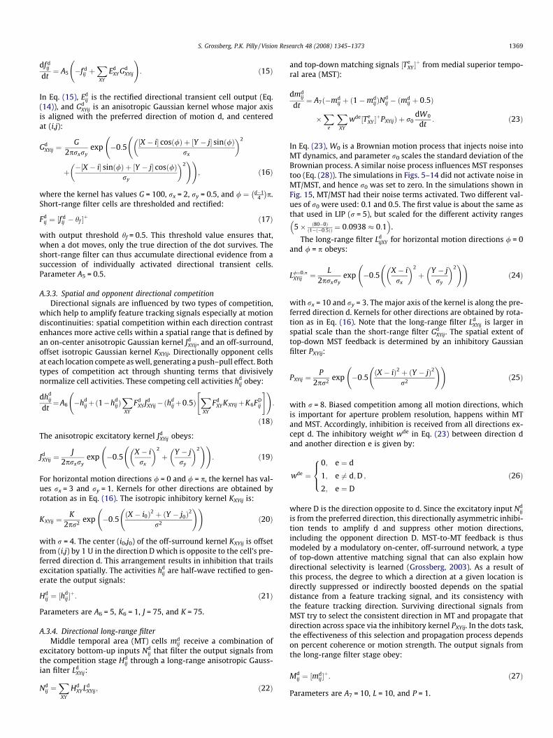
S. Grossberg, P.K. Pilly / Vision Research 48 (2008) 1345–1373 1369
df dij
dt¼ A5 �f d
ij þXXY
EdXY Gd
XYij
!: ð15Þ
In Eq. (15), Edij is the rectified directional transient cell output (Eq.
(14)), and GdXYij is an anisotropic Gaussian kernel whose major axis
is aligned with the preferred direction of motion d, and centeredat (i,j):
GdXYij ¼
G2prxry
exp �0:5½X � i� cosð/Þ þ ½Y � j� sinð/Þ
rx
� �2
þ �½X � i� sinð/Þ þ ½Y � j� cosð/Þry
� �2!!
; ð16Þ
where the kernel has values G = 100, rx = 2, ry = 0.5, and / ¼ d�14
� �p.
Short-range filter cells are thresholded and rectified:
Fdij ¼ ½f d
ij � hf �þ ð17Þ
with output threshold hf = 0.5. This threshold value ensures that,when a dot moves, only the true direction of the dot survives. Theshort-range filter can thus accumulate directional evidence from asuccession of individually activated directional transient cells.Parameter A5 = 0.5.
A.3.3. Spatial and opponent directional competitionDirectional signals are influenced by two types of competition,
which help to amplify feature tracking signals especially at motiondiscontinuities: spatial competition within each direction contrastenhances more active cells within a spatial range that is defined byan on-center anisotropic Gaussian kernel Jd
XYij, and an off-surround,offset isotropic Gaussian kernel KXYij. Directionally opponent cellsat each location compete as well, generating a push–pull effect. Bothtypes of competition act through shunting terms that divisivelynormalize cell activities. These competing cell activities hd
ij obey:
dhdij
dt¼A6 �hd
ijþð1�hdijÞXXY
FdXY Jd
XYij�ðhdijþ0:5Þ
XXY
FdXY KXYijþK6FD
ij
" # !:
ð18Þ
The anisotropic excitatory kernel JdXYij obeys:
JdXYij ¼
J2prxry
exp �0:5X � irx
� �2
þ Y � jry
� �2 ! !
: ð19Þ
For horizontal motion directions / = 0 and / = p, the kernel has val-ues rx = 3 and ry = 1. Kernels for other directions are obtained byrotation as in Eq. (16). The isotropic inhibitory kernel KXYij is:
KXYij ¼K
2pr2 exp �0:5ðX � i0Þ2 þ ðY � j0Þ
2
r2
! !ð20Þ
with r = 4. The center (i0,j0) of the off-surround kernel KXYij is offsetfrom (i,j) by 1 U in the direction D which is opposite to the cell’s pre-ferred direction d. This arrangement results in inhibition that trailsexcitation spatially. The activities hd
ij are half-wave rectified to gen-erate the output signals:
Hdij ¼ ½h
dij�þ: ð21Þ
Parameters are A6 = 5, K6 = 1, J = 75, and K = 75.
A.3.4. Directional long-range filterMiddle temporal area (MT) cells md
ij receive a combination ofexcitatory bottom-up inputs Nd
ij that filter the output signals fromthe competition stage Hd
ij through a long-range anisotropic Gauss-ian filter Ld
XYij:
Ndij ¼
XXY
HdXY Ld
XYij; ð22Þ
and top-down matching signals ½TeXY �þ from medial superior tempo-
ral area (MST):
dmdij
dt¼ A7ð�md
ij þ ð1�mdijÞN
dij � ðmd
ij þ 0:5Þ
�X
e
XXY
wde½TeXY �þPXYijÞ þ r0
dW0
dt: ð23Þ
In Eq. (23), W0 is a Brownian motion process that injects noise intoMT dynamics, and parameter r0 scales the standard deviation of theBrownian process. A similar noise process influences MST responsestoo (Eq. (28)). The simulations in Figs. 5–14 did not activate noise inMT/MST, and hence r0 was set to zero. In the simulations shown inFig. 15, MT/MST had their noise terms activated. Two different val-ues of r0 were used: 0.1 and 0.5. The first value is about the same asthat used in LIP (r = 5), but scaled for the different activity ranges
5� ð80�0Þð1�ð�0:5ÞÞ ¼ 0:0938 � 0:1
� �.
The long-range filter LdijXY for horizontal motion directions / = 0
and / = p obeys:
L/¼0;pXYij ¼
L2prxry
exp �0:5X � irx
� �2
þ Y � jry
� �2 ! !
ð24Þ
with rx = 10 and ry = 3. The major axis of the kernel is along the pre-ferred direction d. Kernels for other directions are obtained by rota-tion as in Eq. (16). Note that the long-range filter Ld
XYij is larger inspatial scale than the short-range filter Gd
XYij. The spatial extent oftop-down MST feedback is determined by an inhibitory Gaussianfilter PXYij:
PXYij ¼P
2pr2 exp �0:5ðX � iÞ2 þ ðY � jÞ2
r2
! !ð25Þ
with r = 8. Biased competition among all motion directions, whichis important for aperture problem resolution, happens within MTand MST. Accordingly, inhibition is received from all directions ex-cept d. The inhibitory weight wde in Eq. (23) between direction dand another direction e is given by:
wde ¼0; e ¼ d
1; e 6¼ d;D
2; e ¼ D
8><>: ; ð26Þ
where D is the direction opposite to d. Since the excitatory input Ndij
is from the preferred direction, this directionally asymmetric inhibi-tion tends to amplify d and suppress other motion directions,including the opponent direction D. MST-to-MT feedback is thusmodeled by a modulatory on-center, off-surround network, a typeof top-down attentive matching signal that can also explain howdirectional selectivity is learned (Grossberg, 2003). As a result ofthis process, the degree to which a direction at a given location isdirectly suppressed or indirectly boosted depends on the spatialdistance from a feature tracking signal, and its consistency withthe feature tracking direction. Surviving directional signals fromMST try to select the consistent direction in MT and propagate thatdirection across space via the inhibitory kernel PXYij. In the dots task,the effectiveness of this selection and propagation process dependson percent coherence or motion strength. The output signals fromthe long-range filter stage obey:
Mdij ¼ ½md
ij�þ: ð27Þ
Parameters are A7 = 10, L = 10, and P = 1.

1370 S. Grossberg, P.K. Pilly / Vision Research 48 (2008) 1345–1373
A.3.5. Directional groupingMST activity Td
ij is described by
dTdij
dt¼A8 �Td
ijþð1�TdijÞC8Md
ij�ðTdijþ0:5Þ
Xe
XXY
wde½TeXY �þPXYij
!
þr0dW0
dt: ð28Þ
In Eq. (28), the bottom-up input Mdij is the rectified MT output.
Recurrent MST inhibitory connections help to select a winningdirection to be fed back to MT. The spatial extent and directionalasymmetry of this inhibitory interaction are again defined by kernelPXYij and weighting coefficients wde in Eqs. (25) and (26), respec-tively. Parameters are A8 = 10 and C8 = 10. As in Eq. (23), MST wassubjected to cellular noise via term W0 in the simulations reportedin Fig. 15.
The self-normalizing directional activities in MT and MST aresensitive to the ambiguity inherent in the random dot motionstimulus, as shown by model simulations (see Fig. 11). They arespatially distributed, as are the moving dots that excite them. LIPprocessing receives these spatially distributed directional signalsand converts them into probabilistic directional eye movementcommands, as follows.
A.3.6. Decision cells and decision gatingLateral intraparietal area (LIP) firing rate dynamics are related
to the speed and accuracy of perceptual decisions in random dotmotion direction discrimination tasks. LIP shows decision-relatedactivity because monkeys have been trained to communicate theirdecision about the motion direction with an eye movement to theappropriate choice target. LIP is known to be an association area,where visual, cognitive, and saccadic signals all play a role. Wemodel two LIP populations representing the two choice targetsusing a recurrent competitive field (RCF). The LIP equation forthe RT task (Roitman & Shadlen, 2002) is as follows:
dyd
dt¼ � A9yd þ ðB9 � ydÞ kSd þ TC þ gdf ðydÞ þ Gd½ � � yd½g2hðyDÞ þ GI�
þ rdWdt
; ð29Þ
where yd is the activity of the LIP population that codes direction d,Sd represents the population activity of the foveal MST pool tuned todirection d, namely:
Sd ¼XXY
½TdXY �þ; ð30Þ
TC is the bottom-up input due to the presence of the visual targetwithin the receptive field of each LIP population, f(yd) is the recurrenton-center feedback signal, Gd is an excitatory, higher level inputwhich is only invoked to make a forced choice, especially after a rea-sonable time has elapsed without a decision, yD is the activity of theLIP population with the opponent motion preference, h(yD) is therecurrent off-surround feedback signal, GI is an inhibitory, higher le-vel signal which causes inhibition after the eyes start moving, W is aBrownian motion process that simulates the stochastic componentsof LIP activity, r2 scales the variance of the Brownian motion process,and gd and g2 are gains of the recurrent on-center and off-surroundterms, respectively. The value of the visual signal TC is chosen so thatthe two LIP population activities equilibrate at an activity h before theonset of the dots, as in the data:
TC ¼h½A9 þ g2hðhÞ�
B9 � h� gdf ðhÞ: ð31Þ
The above-baseline activity h is attributed to the presence of thechoice target within the receptive field of the LIP population. Theexcitatory recurrent signal is defined by:
f ðxÞ ¼ xn
ln þ xn: ð32Þ
Basal ganglia (BG) gate both the competing saccade plans from real-ization. When the activity of either population (say direction d)reaches the decision threshold C1, the BG are assumed to open amovement gate that switches the gain gd to gBG. As a result, the activ-ity of that population is rapidly amplified, thereby simulating thepre-saccadic enhancement in activity seen for about 100 ms beforethe eyes start moving. The inhibitory recurrent signal is defined by:
hðxÞ ¼ xm
lm þ xm: ð33Þ
Parameters are A9 = 1, B9 = 80, k ¼ 560�60 ¼ 1:39� 10�3, gd = 2, g2 = 5,
gBG = 10, l = 50, n = 5, m = 10, C1 = 55, r = 5, and h = 35 (estimatedfrom data).
Inputs Gd and GI in Eq. (29) are initially equal to zero. Wheneither activity (yd or yD) reaches C2 = 70 (see Figs. 7, 9, and 11 inRoitman & Shadlen, 2002), the eyes begin to move, as can be seenin the data. Post-saccadic suppression from FEF post-saccadic cellsnow comes into play by turning GI on from 0 to 30. Reaction time(RT) in each trial is recorded as the time from motion onset untilwhen either activity yd or yD crosses C2; that is, when the choicesaccade is actually initiated. The random dot motion display turnsoff upon saccade onset. We assume post-saccadic suppression, anddecay due to loss of sensory inputs, reset LIP activities to zero be-fore a new trial begins. The value for the parameter B9 is chosen asC2 + 10, so that the LIP cell activity yd can exceed criterion level C2.The value of C1 is also chosen from data by identifying the level offiring in the RT task for correct Tin choices, after which differencesin input motion strength do not seem to play a role.
Sometimes, neither activity can reach threshold C1 in a reason-able time (about 1 s). The model is then forced to make a choice, asfollows: if for some random time between 1000 ms and 1100 ms,the model has not taken a decision, then the direction d corre-sponding to the greater LIP activity is chosen by turning on Gd from0 to 2gd. Simulations done without this volitional mechanism atwork are reported in Fig. 13.
Since the Brownian motion process W(t) in Eq. (29) is an inde-pendent increments process, the increments [W(t) �W(s)] arezero-mean, Gaussian random variables with variance t � s fort > s. Thus at each time step (Dt = 0.001s) of numerical integration,a zero-mean, Gaussian random variable of variance r2Dt is addedto the evolving LIP activity. The same is true in Eq. (34) below.
The FD task simulations use the same equation:
dyd
dt¼ �A9yd þ ðB9 � ydÞ½kSd þ TC þ gdf ðydÞ� � yd½g2hðyDÞ þ GI�
þ rdWdt
: ð34Þ
The various parameters here have the same meaning as those de-scribed for the RT task. Experimental data from two FD tasks (Roit-man & Shadlen, 2002; Shadlen & Newsome, 2001) are simulated.First, we model the 2002 FD task which was done on the same ma-caques in alternating blocks of trials with the RT task. In this task,the dots turn off after 1 s of viewing. The monkey needs to makea choice based on all evidence accumulated in the 1 s. Thus, themodel monkey basically chooses that direction with the greaterLIP activity at the end of the motion viewing period. The passive de-cay rate A9 is given a slightly higher value (4.5) for the FD task; seeSection 3.2. In the 2002 FD task, the monkeys have to remembertheir choice during an ensuing delay period, whose duration is var-ied randomly between 500 ms and 1500 ms, before the fixationpoint is extinguished, which cues the monkey to go ahead withthe chosen saccade. This is enabled by a jump in the recurrenton-center gain gd of the judged direction d to gdelay at the end ofthe motion stimulus viewing period. As a result, activity yd is pre-
S. Grossberg, P.K. Pilly / Vision Research 48 (2008) 1345–1373 1371
vented from being attenuated during the delay period, and alsobuilds up slowly, as observed in the data. When the fixation pointturns off, the basal ganglia are assumed to open the gate for theappropriate saccade plan, which results in the typical pre-saccadicenhancement in activity. This is realized by a further, instant gainboost for the on-center gain gd to gBG. Post-saccadic inhibition istriggered when yd crosses C2 = 70 by turning on GI from 0 to 30 justas in the RT task. Parameters gdelay and gBG are 9 and 35.
The 2001 FD task recorded from different monkeys and hencedifferent LIP populations. The LIP responses during the task weretherefore somewhat different, for example in the dynamic rangeof firing (0 � C2 Hz), and in the above-baseline firing due to thepresence of the target before the onset of dots (h). Accordingly,the simulated LIP decision circuit was the same as that of the2002 FD task, but some parameters were not: A9 = 5, B9 = 60,k ¼ 3
60�60 ¼ 8:33� 10�4, gd = 2, g2 = 7.5, l = 25, n = 5, m = 10, r = 5,h = 15, C2 = 50. The values for h and C2 were again chosen from data(see Figs. 8 and 12 in Shadlen & Newsome, 2001), and B9 = C2 + 10.In this FD task, the delay period duration is randomly chosen be-tween 200 ms and 2000 ms. The recurrent on-center gain gd asso-ciated with the chosen direction d jumps from 2 to 5.5 (gdelay) atthe start of the delay period, and then to 25 (gBG) when the FP isturned off. As in the other task simulations, post-saccadic inhibi-tion begins when yd crosses C2, which turns on GI from 0 to 30.
A.4. Psychometric function
For each task, the simulated proportion correct data, p(C), de-fined to be the fraction out of 500 trials at each percent coherenceC, is fit with a cumulative Weibull distribution function for two-alternative, forced choice tasks:
pðCÞ ¼ 12þ 1
21� exp � C
a
� �b" # !
ð35Þ
using a maximum likelihood estimation procedure presented inMyung (2003). Parameter a is the threshold of the psychometricfunction, and corresponds to the coherence level that elicits �82%accuracy. Parameter b controls the steepness of the psychometricfunction. Since there are just two alternatives, the Weibull functionyields a chance performance of 0.5, or 50%, at 0% coherencepð0Þ ¼ 1
2
� �.
References
Albright, T. D., Desimone, R., & Gross, C. G. (1984). Columnar organization ofdirectionally sensitive cells in visual area MT of the macaque. Journal ofNeurophysiology, 51, 16–31.
Anstis, S. M. (1970). Phi movement as a subtraction process. Vision Research, 10,1411–1430.
Anstis, S. M., & Rogers, B. J. (1975). Illusory reversals of visual depth and movementduring changes in contrast. Vision Research, 15, 957–961.
Baloch, A. A., & Grossberg, S. (1997). A neural model of high-level motionprocessing: Line motion and formotion dynamics. Vision Research, 37,3037–3059.
Baloch, A. A., Grossberg, S., Mingolla, E., & Nogueira, C. A. M. (1999). Neural model offirst-order and second-order motion perception and magnocellular dynamics.Journal of the Optical Society of America A: Optics, Image Science, and Vision, 16,953–978.
Barlow, H. B., & Levick, W. R. (1965). The mechanism of directionally selective unitsin the rabbit’s retina. Journal of Physiology, 178, 477–504.
Basso, M. A., & Wurtz, R. H. (1998). Modulation of neuronal activity in superiorcolliculus by changes in target probability. Journal of Neuroscience, 18,7519–7534.
Ben-Av, M. B., & Shiffrar, M. (1995). Disambiguating velocity estimates across imagespace. Vision Research, 35, 2889–2895.
Berzhanskaya, J., Grossberg, S., & Mingolla, E. (2007). Laminar cortical dynamics ofvisual form and motion interactions during coherent object motion perception.Spatial Vision, 20, 337–395.
Bichot, N. P., & Schall, J. D. (1996). Visual feature selectivity in frontal eye fieldsinduced by experience in mature macaques. Nature, 381, 697–699.
Bisley, J. W., & Goldberg, M. E. (2003). Neuronal activity in the lateral intraparietalarea and spatial attention. Science, 299, 81–86.
Bisley, J. W., Krishna, B. S., & Goldberg, M. E. (2004). A rapid and precise on-responsein posterior parietal cortex. Journal of Neuroscience, 24, 1833–1838.
Boardman, I., Grossberg, S., Myers, C., & Cohen, M. (1999). Neural dynamics ofperceptual order and context effects for variable-rate speech syllables.Perception & Psychophysics, 6, 1477–1500.
Born, R. T. (2004). Taking strategies to task. Neuron, 42, 185–187.Bowns, L. (1996). Evidence for a feature tracking explanation of why type II plaids
move in the vector sum direction at short durations. Vision Research, 36,3685–3694.
Bowns, L. (2001). IOC, vector sum, and squaring: Three different motion effects orone? Vision Research, 41, 965–972.
Britten, K. H., Newsome, W. T., Shadlen, M. N., Celebrini, S., & Movshon, J. A. (1996).A relationship between behavioral choice and the visual responses of neurons inmacaque MT. Visual Neuroscience, 13, 87–100.
Britten, K. H., Shadlen, M. N., Newsome, W. T., & Movshon, J. A. (1993). Responses ofneurons in macaque MT to stochastic motion signals. Visual Neuroscience, 10,1157–1169.
Brown, J. W., Bullock, D., & Grossberg, S. (2004). How laminar frontal cortex andbasal ganglia circuits interact to control planned and reactive saccades. NeuralNetworks, 17, 471–510.
Bruce, C. J., Goldberg, M. E., Bushnell, M. C., & Stanton, G. B. (1985). Primate frontaleye fields: II. Physiological and anatomical correlates of electrically-evoked eyemovements. Journal of Neurophysiology, 54, 714–734.
Busemeyer, J. R., & Townsend, J. T. (1993). Decision field theory. PsychologicalReview, 100, 432–459.
Castet, E., Lorenceau, J., Shiffrar, M., & Bonnet, C. (1993). Perceived speed of movinglines depends on orientation, length, speed and luminance. Vision Research, 33,1921–1936.
Celebrini, S., & Newsome, W. T. (1994). Neuronal and psychophysical sensitivity tomotion signals in extrastriate MST of the macaque monkey. Journal ofNeuroscience, 14, 4109–4124.
Celebrini, S., & Newsome, W. T. (1995). Microstimulation of extrastriate area MSTinfluences performance on a direction discrimination task. Journal ofNeurophysiology, 73, 437–448.
Chey, J., Grossberg, S., & Mingolla, E. (1997). Neural dynamics of motion grouping:From aperture ambiguity to object speed and direction. Journal of the OpticalSociety of America A: Optics, Image Science, and Vision, 14, 2570–2594.
Chey, J., Grossberg, S., & Mingolla, E. (1998). Neural dynamics of motion processingand speed discrimination. Vision Research, 38, 2769–2786.
Chubb, C., & Sperling, G. (1989). Two motion perception mechanisms revealedthrough distance-driven reversal of apparent motion. Proceedings of the NationalAcademy of Sciences of the United States of America, 86, 2985–2989.
Churchland, A. K., Kiani, R., & Shadlen, M. N. (2007). LIP neurons combineaccumulated evidence with a representation of elapsed time—urgency—tomediate a perceptual decision. Society of Neuroscience Abstracts, 507.3.
Churchland, A. K., Tam, M., Plamer, J., Kiani, R., & Shadlen, M. N. (2005). Responses ofLIP neurons reflect accumulation of evidence in a multiple choice decision task.Society of Neuroscience Abstracts, 16.8.
Cisek, P. (2006). Integrated neural processes for defining potential actions anddeciding between them: A computational model. Journal of Neuroscience, 26,9761–9770.
Cisek, P., & Kalaska, J. F. (2005). Neural correlates of reaching decisions in dorsalpremotor cortex: Specification of multiple direction choices and final selectionof action. Neuron, 45, 801–814.
Ditterich, J. (2006a). Stochastic models of decisions about motion direction:Behavior and physiology. Neural Networks, 19, 981–1012.
Ditterich, J. (2006b). Evidence for time-variant decision making. European Journal ofNeuroscience, 24, 3628–3641.
Ditterich, J., Mazurek, M., & Shadlen, M. N. (2003). Microstimulation of visual cortexaffects the speed of perceptual decisions. Nature Neuroscience, 6, 891–898.
Egeth, H. E., & Yantis, S. (1997). Visual attention: Control, representation and timecourse. Annual Review of Psychology, 48, 269–297.
Francis, G., & Grossberg, S. (1996a). Cortical dynamics of boundary segmentationand reset: Persistence, afterimages and residual traces. Perception, 35, 543–567.
Francis, G., & Grossberg, S. (1996b). Cortical dynamics of form and motionintegration: Persistence, apparent motion, and illusory contours. VisionResearch, 36, 149–173.
Francis, G., Grossberg, S., & Mingolla, E. (1994). Cortical dynamics of feature bindingand reset: Control of visual persistence. Vision Research, 34, 1089–1104.
Freedman, D. J., & Assad, J. A. (2006). Experience-dependent representation of visualcategories in parietal cortex. Nature, 443, 85–88.
Fried, S. I., Münch, T. A., & Werblin, F. S. (2002). Mechanisms and circuitryunderlying directional selectivity in the retina. Nature, 420, 411–414.
Gancarz, G., & Grossberg, G. (1998). A neural model of the saccade generator in thereticular formation. Neural Networks, 11, 1159–1174.
Gancarz, G., & Grossberg, S. (1999). A neural model of saccadic eye movementcontrol explains task-specific adaptation. Vision Research, 39, 3123–3143.
Glimcher, P. W. (2003). The neurobiology of visual-saccadic decision making.Annual Review of Neuroscience, 26, 133–179.
Gold, J. I., & Shadlen, M. N. (2001). Neural computations that underlie decisionsabout sensory stimuli. Trends in Cognitive Sciences, 5, 10–16.
Gold, J. I., & Shadlen, M. N. (2003). The influence of behavioral context on therepresentation of a perceptual decision in developing oculomotor commands.Journal of Neuroscience, 23, 632–651.
Gold, J. I., & Shadlen, M. N. (2007). The neural basis of decision-making. AnnualReview of Neuroscience, 30, 535–574.
1372 S. Grossberg, P.K. Pilly / Vision Research 48 (2008) 1345–1373
Grossberg, S. (1972). A neural theory of punishment and avoidance: II. Quantitativetheory. Mathematical Biosciences, 15, 253–285.
Grossberg, S. (1973). Contour enhancement, short term memory, and constancies inreverberating neural networks. Studies in Applied Mathematics, 52, 213–257.
Grossberg, S. (1978). A theory of human memory: Self-organization andperformance of sensory-motor codes, maps, and plans. In R. Rosen & F. Snell(Eds.). Progress in theoretical biology (Vol. 5, pp. 233–374). New York, NY:Academic.
Grossberg, S. (1980). How does a brain build a cognitive code? Psychological Review,87, 1–51.
Grossberg, S. (1988). Nonlinear neural networks: Principles, mechanisms, andarchitectures. Neural Networks, 1, 17–61.
Grossberg, S. (2003). How does the cerebral cortex work? Development, learning,attention, and 3D vision by laminar circuits of visual cortex. Behavioral andCognitive Neuroscience Reviews, 2, 47–76.
Grossberg, S., & Myers, C. W. (2000). The resonant dynamics of speech perception:Interword integration and duration-dependent backward effects. PsychologicalReview, 107, 735–767.
Grossberg, S., Boardman, I., & Cohen, C. (1997). Neural dynamics of variable-ratespeech categorization. Journal of Experimental Psychology: Human Perception andPerformance, 23, 418–503.
Grossberg, S., Mingolla, E., & Viswanathan, L. (2001). Neural dynamics of motionintegration and segmentation within and across apertures. Vision Research, 41,2521–2553.
Grossberg, S., Roberts, K., Aguilar, M., & Bullock, D. (1997). A neural model ofmultimodal adaptive saccadic eye movement control by superior colliculus.Journal of Neuroscience, 17, 9706–9725.
Grossberg, S., & Rudd, M. E. (1989). A neural architecture for visual motionperception: Group and element apparent motion. Neural Networks, 2, 421–450.
Grossberg, S., & Rudd, M. E. (1992). Cortical dynamics of visual motion perception:Short-range and long-range apparent motion. Psychological Review, 99, 78–121.
Grossberg, S., Srihasam, K., & Bullock, D. (submitted for publication). Neuraldynamics of saccadic and smooth pursuit eye movement coordination duringvisual tracking of unpredictably moving targets.
Heeger, D. G., Boynton, G. M., Demb, J. B., Seidemann, E., & Newsome, W. T. (1999).Motion opponency in visual cortex. Journal of Neuroscience, 19, 7162–7174.
Heekeren, H. R., Marrett, S., Bandettini, P. A., & Ungerleider, L. G. (2004). A generalmechanism for perceptual decision-making in the human brain. Nature, 431,859–862.
Helmholtz, H. (2000). Treatise on physiological optics. Bristol, UK: Thoemmes.Hikosaka, O., & Wurtz, R. H. (1983). Visual and oculomotor functions of monkey
substantia nigra pars reticulata. IV. Relation of substantia nigra to superiorcolliculus. Journal of Neurophysiology, 49, 780–798.
Hikosaka, O., & Wurtz, R. H. (1989). The basal ganglia. In R. Wurtz & M. Goldberg(Eds.), The neurobiology of saccadic eye movements (pp. 257–281). Amsterdam:Elsevier.
Hodgkin, A. L., & Huxley, A. F. (1952). A quantitative description of membranecurrent and its application to conduction and excitation in nerve. Journal ofPhysiology, 117, 500–544.
Horwitz, G. D., Batista, A. P., & Newsome, W. T. (2004a). Direction-selective visualresponses in macaque superior colliculus induced by behavioral training.Neuroscience Letters, 366, 315–319.
Horwitz, G. D., Batista, A. P., & Newsome, W. T. (2004b). Representation of anabstract perceptual decision in macaque superior colliculus. Journal ofNeurophysiology, 91, 2281–2296.
Horwitz, G. D., & Newsome, W. T. (2001a). Target selection for saccadic eyemovements: Direction-selective visual responses in the superior colliculus.Journal of Neurophysiology, 86, 2527–2542.
Horwitz, G. D., & Newsome, W. T. (2001b). Target selection for saccadic eyemovements: Prelude activity in the superior colliculus during a direction-discrimination task. Journal of Neurophysiology, 86, 2543–2558.
Jazayeri, M., & Movshon, J. A. (2006). Optimal representation of sensory informationby neural populations. Nature Neuroscience, 9, 690–696.
Kanizsa, G. (1979). Organization in vision: Essays on gestalt perception. New York, NY:Praeger.
Kaplan, E., & Benardete, E. (2001). The dynamics of primate retinal ganglion cells.Progress in Brain Research, 134, 17–34.
Kersten, D., Mamassian, P., & Yuille, A. (2004). Object perception as Bayesianinference. Annual Review of Psychology, 55, 271–304.
Kersten, D., & Yuille, A. (2003). Bayesian models of object perception. CurrentOpinion in Neurobiology, 13, 1–9.
Kim, J.-N., & Shadlen, M. N. (1999). Neural correlates of a decision in the dorsolateralprefrontal cortex of the macaque. Nature Neuroscience, 2, 176–185.
Knill, D., & Pouget, A. (2004). The Bayesian brain: The role of uncertainty in neuralcoding and computation. Trends in Neuroscience, 27, 712–719.
Li, X., Kim, B., & Basso, M. A. (2006). Transient pauses in delay-period activity ofsuperior colliculus neurons. Journal of Neurophysiology, 95, 2252–2264.
Lorenceau, J., & Gorea, A. (1989). ’Blobs’ are critical in perceiving the direction ofmoving plaids. Perception, 18, 539.
Lorenceau, J., & Shiffrar, M. (1992). The influence of terminators on motionintegration across space. Vision Research, 32, 263–273.
Luce, R. D. (1986). Response times: Their role in inferring elementary mentalorganization. New York, NY: Oxford University.
Ma, W. J., Beck, J. M., Latham, P. E., & Pouget, A. (2006). Bayesian inference withprobabilistic population codes. Nature Neuroscience, 9, 1432–1438.
Mazurek, M. E., Hanks, T., Yang, T., & Shadlen, M. N. (2005). Prior probabilitychanges the rate of evidence accumulation in a motion discrimination task:Behavior and LIP physiology. Society of Neuroscience Abstracts, 621.3.
Mazurek, M. E., Roitman, J. D., Ditterich, J., & Shadlen, M. N. (2003). A role for neuralintegrators in perceptual decision making. Cerebral Cortex, 13, 1257–1269.
Miller, E. K., Erickson, C. A., & Desimone, R. (1996). Neural mechanisms of visualworking memory in prefrontal cortex of the macaque. Journal of Neuroscience,16, 5154–5167.
Mingolla, E., Todd, J. T., & Norman, J. F. (1992). The perception of globally coherentmotion. Vision Research, 32, 1015–1031.
Munoz, D. P., & Wurtz, R. H. (1995a). Saccade-related activity in monkey superiorcolliculus. I. Characteristics of burst and buildup cells. Journal ofNeurophysiology, 73, 2313–2333.
Munoz, D. P., & Wurtz, R. H. (1995b). Saccade-related activity in monkey superiorcolliculus. II. Spread of activity during saccades. Journal of Neurophysiology, 73,2334–2348.
Myung, I. J. (2003). Tutorial on maximum likelihood estimation. Journal ofMathematical Psychology, 47, 90–100.
Nichols, M. J., & Newsome, W. T. (2002). Middle temporal visual areamicrostimulation influences veridical judgments of motion direction. Journalof Neuroscience, 22, 9530–9540.
Pack, C. C., & Born, R. T. (2001). Temporal dynamics of a neural solution to theaperture problem in area MT of macaque brain. Nature, 409, 1040–1042.
Palmer, J., Huk, A., & Shadlen, M. N. (2005). The effect of stimulus strength on thespeed and accuracy of a perceptual decision. Journal of Vision, 5, 376–404.
Pilly, P. K., & Grossberg, S. (2005). Brain without Bayes: Temporal dynamics ofdecision-making in the laminar circuits of visual cortex. Society of NeuroscienceAbstracts, 591.1.
Pilly, P. K., & Grossberg, S. (2006). Brain without Bayes: Temporal dynamics ofdecision-making during form and motion perception by the laminar circuits ofvisual cortex. Journal of Vision, 6, 886.
Platt, M. L. (2002). Neural correlates of decisions. Current Opinion in Neurobiology,12, 141–148.
Pouget, A., Dayan, P., & Zemel, R. S. (2003). Computation and inference withpopulation codes. Annual Review of Neuroscience, 26, 381–410.
Rao, R. (2004). Bayesian computation in recurrent neural circuits. NeuralComputation, 16, 1–38.
Ratcliff, R. (1978). A theory of memory retrieval. Psychological Review, 85, 59–108.Ratcliff, R. (1980). A note on modeling accumulation of information when the rate of
accumulation changes over time. Journal of Mathematical Psychology, 21,178–184.
Ratcliff, R., Cherian, A., & Segraves, M. (2003). A comparison of macaque behaviorand superior colliculus neuronal activity to predictions from models of simpletwo-choice decisions. Journal of Neurophysiology, 90, 1392–1407.
Ratcliff, R., van Zandt, T., & McKoon, G. (1999). Connectionist and diffusion modelsof reaction time. Psychological Review, 106, 261–300.
Ratcliff, R., & Rouder, J. N. (1998). Modeling response times for two-choicedecisions. Psychological Science, 9, 347–356.
Ratcliff, R., & Smith, P. L. (2004). A comparison of sequential sampling models fortwo-choice reaction time. Psychological Review, 111, 333–367.
Reddi, B. A. J., & Carpenter, R. H. S. (2000). The influence of urgency on decision time.Nature Neuroscience, 3, 827–830.
Roitman, J. D., & Shadlen, M. N. (2002). Response of neurons in the lateralintraparietal area during a combined visual discrimination reaction time task.Journal of Neuroscience, 22, 9475–9489.
Romo, R., & Salinas, E. (2001). Touch and go: Decision-making mechanisms insomatosensation. Annual Review of Neuroscience, 24, 107–137.
Salzman, C. D., Murasugi, C. M., Britten, K. H., & Newsome, W. T. (1992).Microstimulation in visual area MT: Effects on direction discriminationperformance. Journal of Neuroscience, 2, 2331–2355.
Schall, J. D. (2003). Neural correlates of decision processes: Neural and mentalchronometry. Current Opinion in Neurobiology, 13, 182–186.
Schiller, P. H. (1992). The ON and OFF channels of the visual system. Trends inNeuroscience, 15, 86–92.
Shadlen, M. N., & Newsome, W. T. (2001). Neural basis of a perceptual decision inthe parietal cortex (area LIP) of the rhesus monkey. Journal of Neurophysiology,86, 1916–1936.
Smith, P. L. (1990). A note on the distribution of response times for a random walkwith Gaussian increments. Journal of Mathematical Psychology, 34, 445–459.
Smith, P. L. (2000). Stochastic dynamic models of response time and accuracy: Afoundational primer. Journal of Mathematical Psychology, 44, 408–463.
Smith, P. L., & Ratcliff, R. (2004). Psychology and neurobiology of simple decisions.Trends in Neurosciences, 27, 161–168.
Smith, P. L., & Vickers, D. (1988). The accumulator model of two-choicediscrimination. Journal of Mathematical Psychology, 32, 135–168.
Snowden, R. J., Treue, S., Erickson, R. G., & Andersen, R. A. (1991). The response ofarea MT and V1 neurons to transparent motion. Journal of Neuroscience, 11,2768–2785.
Srihasam, K., Bullock, D., & Grossberg, S. (2008). Target selection by frontal cortexduring coordinated saccadic and smooth pursuit eye movements. Journal ofCognitive Neuroscience, in press.
Stocker, A. A., & Simoncelli, E. P. (2006). Noise characteristics and prior expectationsin human visual speed perception. Nature Neuroscience, 9, 578–585.
Thorpe, S., Fize, D., & Marlot, C. (1996). Speed of processing in the human visualsystem. Nature, 381, 520–522.

S. Grossberg, P.K. Pilly / Vision Research 48 (2008) 1345–1373 1373
Uka, T., & DeAngelis, G. C. (2004). Contribution of area MT to stereoscopic depthperception: Choice-related response modulations reflect task strategy. Neuron,42, 297–310.
Usher, M., & McClelland, J. L. (2001). The time course of perceptual choice: Theleaky, competing accumulator model. Psychological Review, 108, 550–592.
Wallach, H. (1935). On the visually perceived direction of motion. PsychologischeForschung, 20, 325–380.
Wang, X.-J. (2002). Probabilistic decision making by slow reverberation in corticalcircuits. Neuron, 36, 955–968.
Wong, K.-F., & Wang, X.-J. (2006). A recurrent network mechanism of timeintegration in perceptual decisions. Journal of Neuroscience, 26,1314–1328.
Weiss, Y., Simoncelli, E. P., & Adelson, E. H. (2002). Motion illusions as optimalpercepts. Nature Neuroscience, 5, 598–604.