Viscous Flow in Ducts - Iran University of Science and ... flow in ducts.pdf · Fluid Mechanics I 7...
61
School of Mechanical Engineering Viscous Flow in Ducts Dr. M. Siavashi School of Mechanical Engineering Iran University of Science and Technology Spring 2014
-
Upload
truongdung -
Category
Documents
-
view
229 -
download
0
Transcript of Viscous Flow in Ducts - Iran University of Science and ... flow in ducts.pdf · Fluid Mechanics I 7...
School of Mechanical Engineering
Viscous Flow in Ducts
Dr. M. Siavashi School of Mechanical Engineering
Iran University of Science and Technology
Spring 2014
Viscous Flow in Ducts Fluid Mechanics I 2
School of Mechanical Engineering
Objectives
1. Have a deeper understanding of laminar and
turbulent flow in pipes and the analysis of fully
developed flow
2. Calculate the major and minor losses
associated with pipe flow in piping networks
and determine the pumping power
requirements
Viscous Flow in Ducts Fluid Mechanics I 3
School of Mechanical Engineering
Introduction
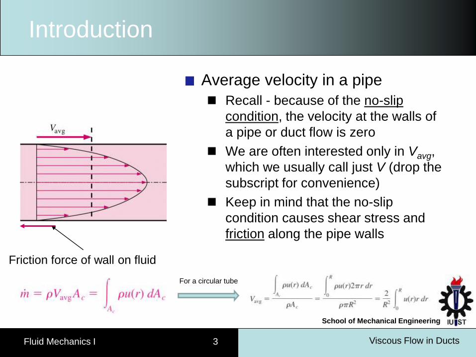
Average velocity in a pipe
Recall - because of the no-slip
condition, the velocity at the walls of
a pipe or duct flow is zero
We are often interested only in Vavg,
which we usually call just V (drop the
subscript for convenience)
Keep in mind that the no-slip
condition causes shear stress and
friction along the pipe walls
Friction force of wall on fluid
For a circular tube
Viscous Flow in Ducts Fluid Mechanics I 4
School of Mechanical Engineering
Introduction
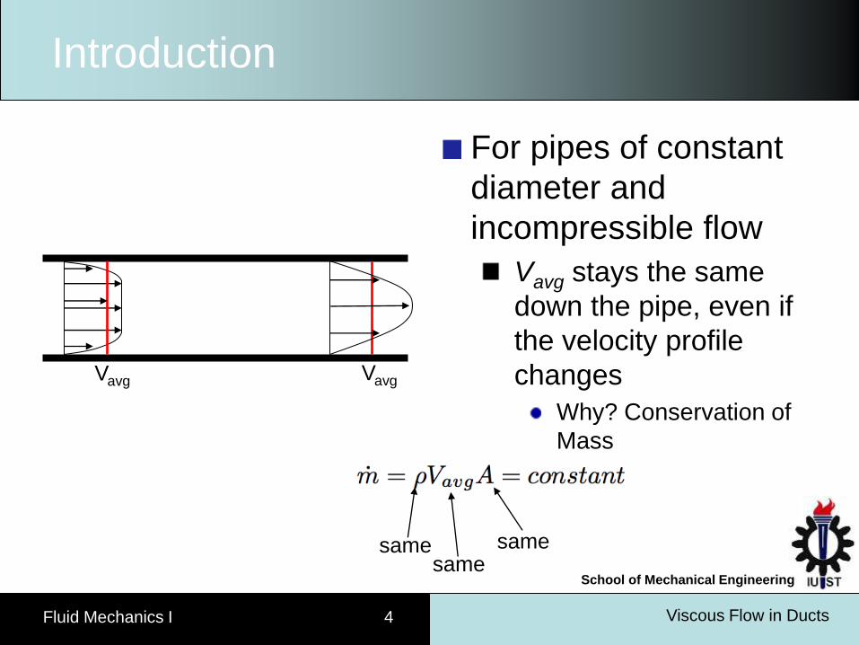
For pipes of constant
diameter and
incompressible flow
Vavg stays the same
down the pipe, even if
the velocity profile
changes
Why? Conservation of
Mass
same
Vavg Vavg
same same
Viscous Flow in Ducts Fluid Mechanics I 5
School of Mechanical Engineering
Introduction
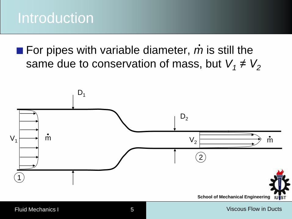
For pipes with variable diameter, m is still the
same due to conservation of mass, but V1 ≠ V2
D2
V2
2
1
V1
D1
m m
Viscous Flow in Ducts Fluid Mechanics I 6
School of Mechanical Engineering
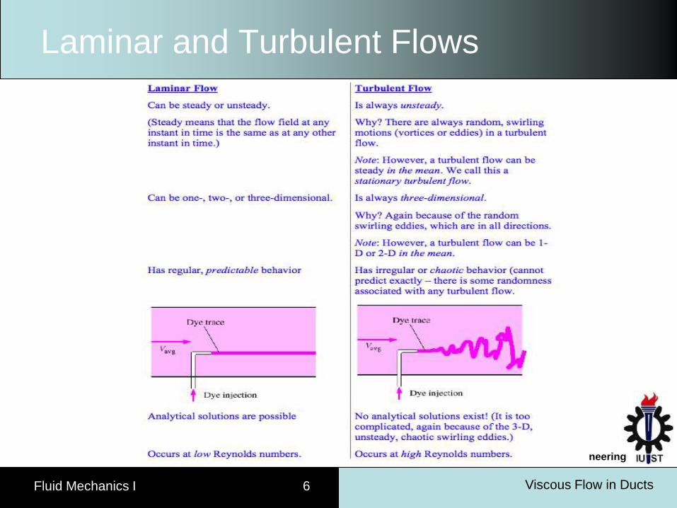
Laminar and Turbulent Flows
Viscous Flow in Ducts Fluid Mechanics I 7
School of Mechanical Engineering
Laminar and Turbulent Flows
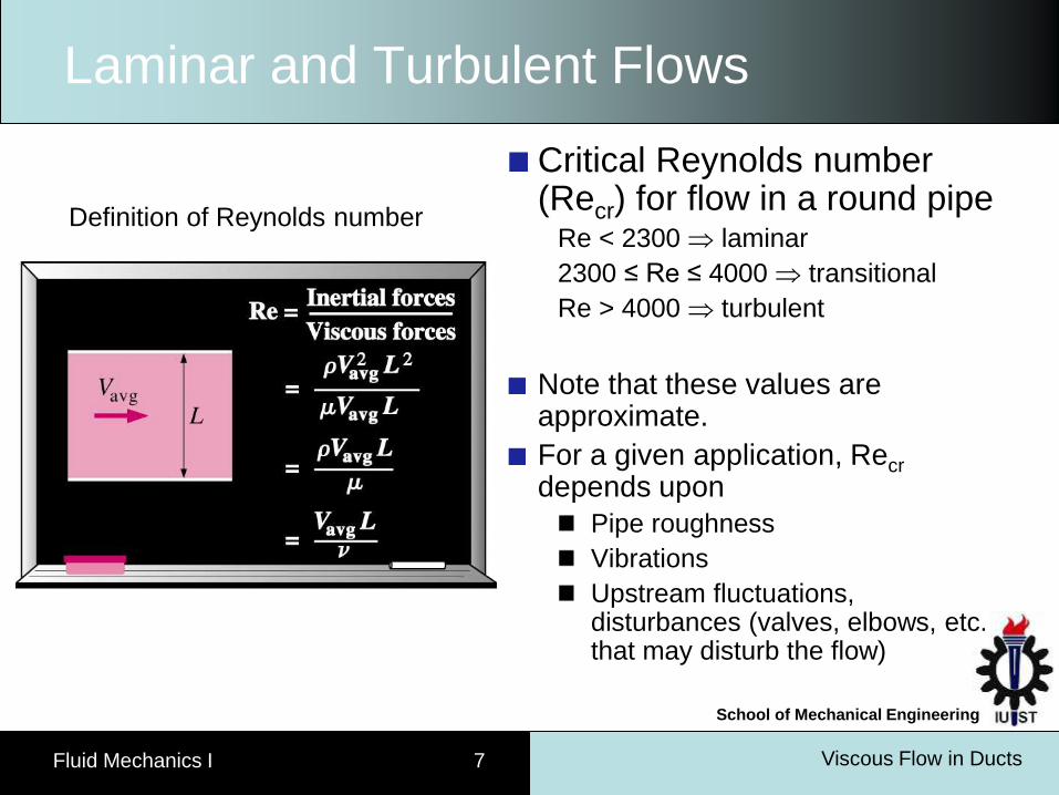
Critical Reynolds number (Recr) for flow in a round pipe
Re < 2300 laminar
2300 ≤ Re ≤ 4000 transitional
Re > 4000 turbulent
Note that these values are approximate.
For a given application, Recr depends upon
Pipe roughness
Vibrations
Upstream fluctuations, disturbances (valves, elbows, etc. that may disturb the flow)
Definition of Reynolds number
Viscous Flow in Ducts Fluid Mechanics I 8
School of Mechanical Engineering
Laminar and Turbulent Flows
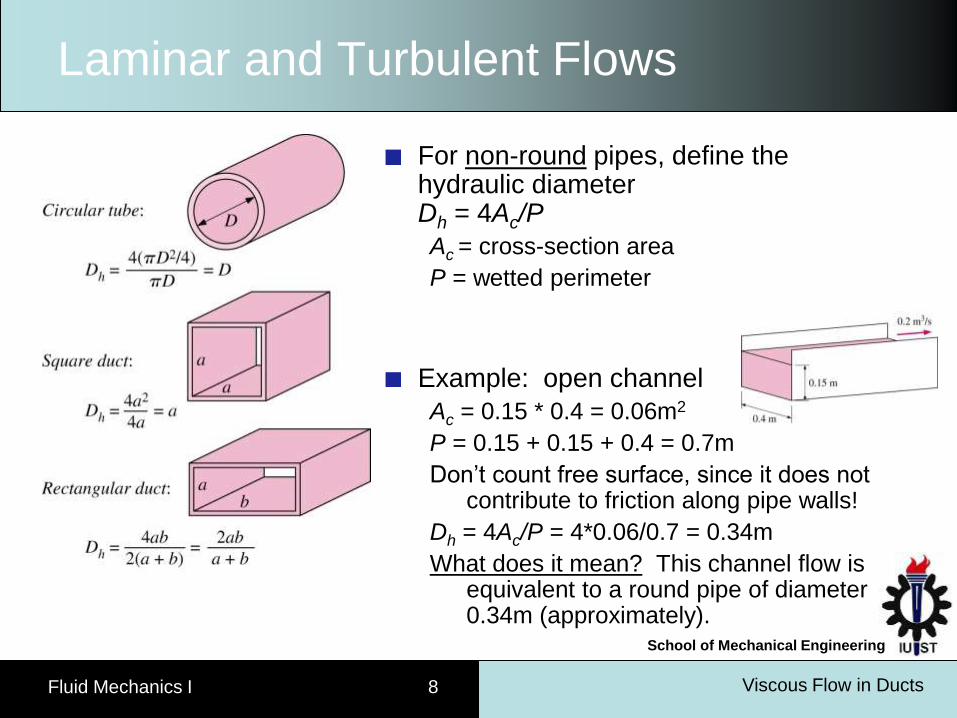
For non-round pipes, define the hydraulic diameter Dh = 4Ac/P
Ac = cross-section area
P = wetted perimeter
Example: open channel
Ac = 0.15 * 0.4 = 0.06m2
P = 0.15 + 0.15 + 0.4 = 0.7m
Don’t count free surface, since it does not contribute to friction along pipe walls!
Dh = 4Ac/P = 4*0.06/0.7 = 0.34m
What does it mean? This channel flow is equivalent to a round pipe of diameter 0.34m (approximately).
Viscous Flow in Ducts Fluid Mechanics I 9
School of Mechanical Engineering
The Entrance Region
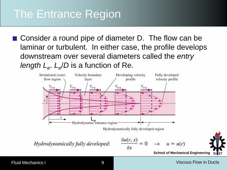
Consider a round pipe of diameter D. The flow can be
laminar or turbulent. In either case, the profile develops
downstream over several diameters called the entry
length Le. Le/D is a function of Re.
Le
Viscous Flow in Ducts Fluid Mechanics I 10
School of Mechanical Engineering
The Entrance Region
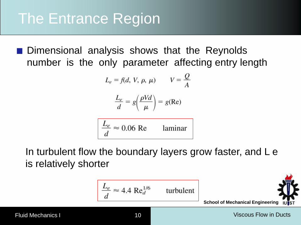
Dimensional analysis shows that the Reynolds
number is the only parameter affecting entry length
In turbulent flow the boundary layers grow faster, and L e
is relatively shorter
Viscous Flow in Ducts Fluid Mechanics I 11
School of Mechanical Engineering
Fully Developed Pipe Flow
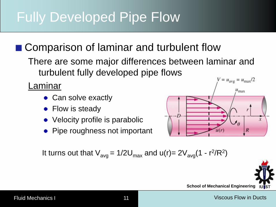
Comparison of laminar and turbulent flow
There are some major differences between laminar and
turbulent fully developed pipe flows
Laminar
Can solve exactly
Flow is steady
Velocity profile is parabolic
Pipe roughness not important
It turns out that Vavg = 1/2Umax and u(r)= 2Vavg(1 - r2/R2)
Viscous Flow in Ducts Fluid Mechanics I 12
School of Mechanical Engineering
Fully Developed Pipe Flow
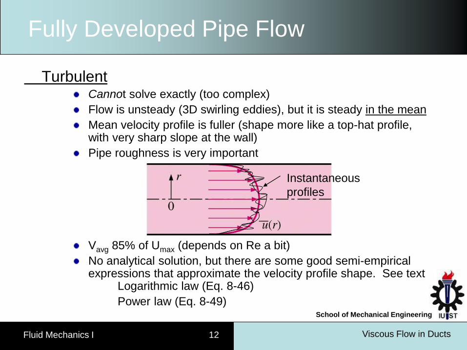
Turbulent Cannot solve exactly (too complex)
Flow is unsteady (3D swirling eddies), but it is steady in the mean
Mean velocity profile is fuller (shape more like a top-hat profile, with very sharp slope at the wall)
Pipe roughness is very important
Vavg 85% of Umax (depends on Re a bit)
No analytical solution, but there are some good semi-empirical expressions that approximate the velocity profile shape. See text Logarithmic law (Eq. 8-46)
Power law (Eq. 8-49)
Instantaneous
profiles
Viscous Flow in Ducts Fluid Mechanics I 13
School of Mechanical Engineering
Fully Developed Pipe Flow
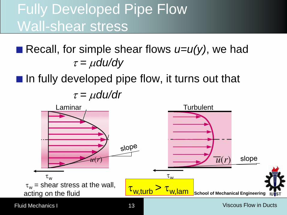
Wall-shear stress
Recall, for simple shear flows u=u(y), we had
= du/dy
In fully developed pipe flow, it turns out that
= du/dr Laminar Turbulent
w w
w,turb > w,lam w = shear stress at the wall,
acting on the fluid
Viscous Flow in Ducts Fluid Mechanics I 14
School of Mechanical Engineering
Fully Developed Pipe Flow
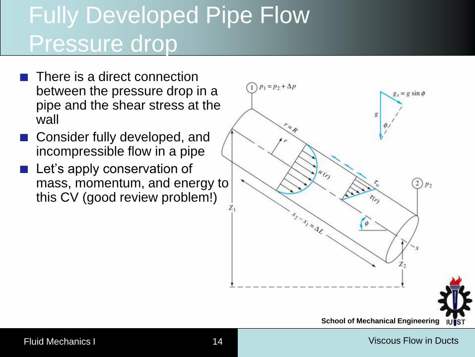
Pressure drop
There is a direct connection between the pressure drop in a pipe and the shear stress at the wall
Consider fully developed, and incompressible flow in a pipe
Let’s apply conservation of mass, momentum, and energy to this CV (good review problem!)
Viscous Flow in Ducts Fluid Mechanics I 15
School of Mechanical Engineering
Fully Developed Pipe Flow
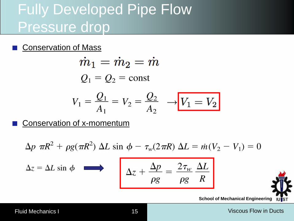
Pressure drop
Conservation of Mass
Conservation of x-momentum
Viscous Flow in Ducts Fluid Mechanics I 16
School of Mechanical Engineering
Fully Developed Pipe Flow
Pressure drop
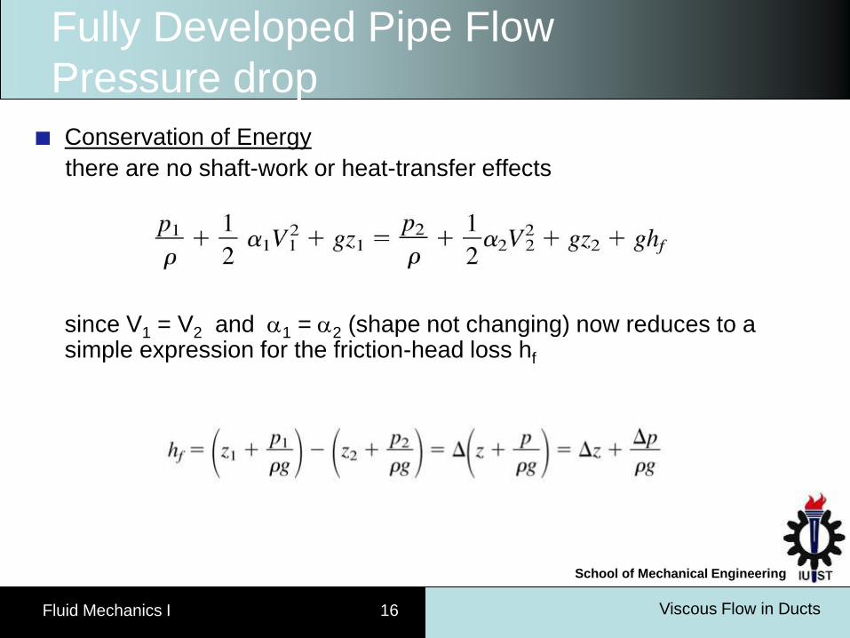
Conservation of Energy
there are no shaft-work or heat-transfer effects
since V1 = V2 and 1 = 2 (shape not changing) now reduces to a simple expression for the friction-head loss hf
Viscous Flow in Ducts Fluid Mechanics I 17
School of Mechanical Engineering
Fully Developed Pipe Flow
Friction Factor
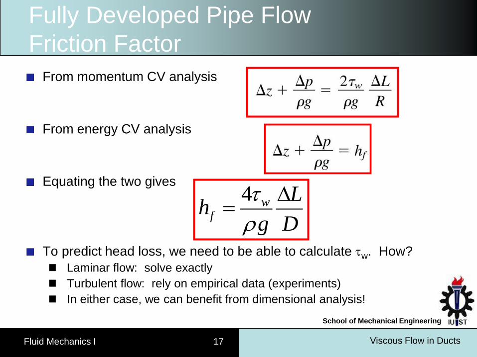
From momentum CV analysis
From energy CV analysis
Equating the two gives
To predict head loss, we need to be able to calculate w. How?
Laminar flow: solve exactly
Turbulent flow: rely on empirical data (experiments)
In either case, we can benefit from dimensional analysis!
4 wf
Lh
g D
Viscous Flow in Ducts Fluid Mechanics I 18
School of Mechanical Engineering
Fully Developed Pipe Flow
Friction Factor
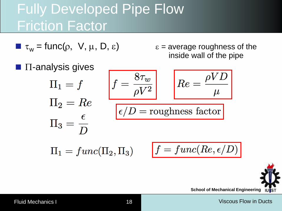
w = func( V, , D, ) = average roughness of the inside wall of the pipe
-analysis gives
Viscous Flow in Ducts Fluid Mechanics I 19
School of Mechanical Engineering
Fully Developed Pipe Flow
Friction Factor
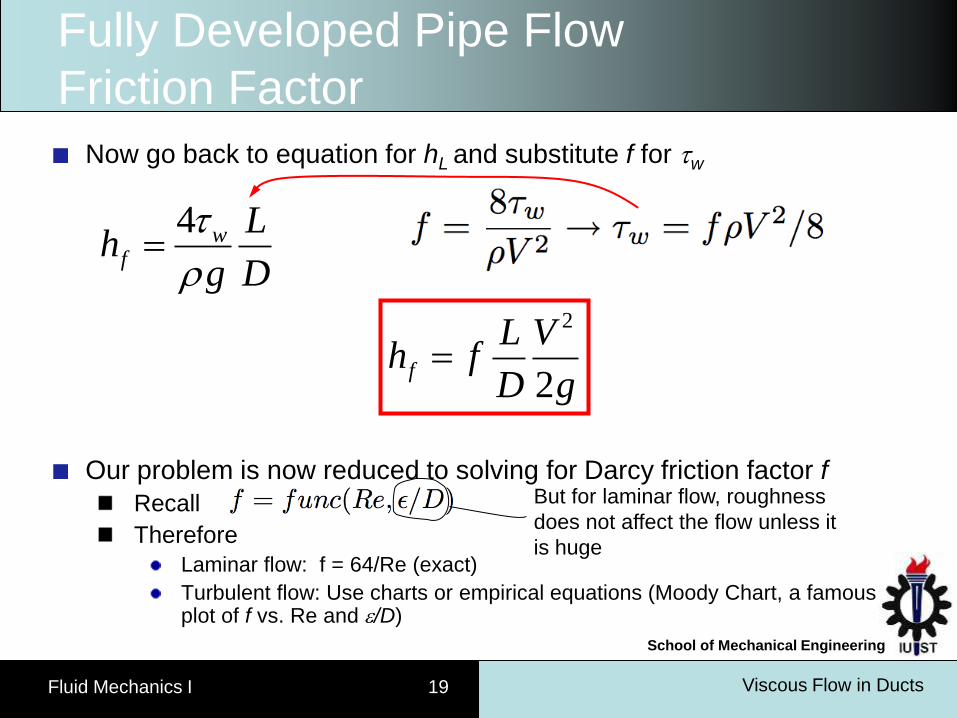
Now go back to equation for hL and substitute f for w
Our problem is now reduced to solving for Darcy friction factor f
Recall
Therefore
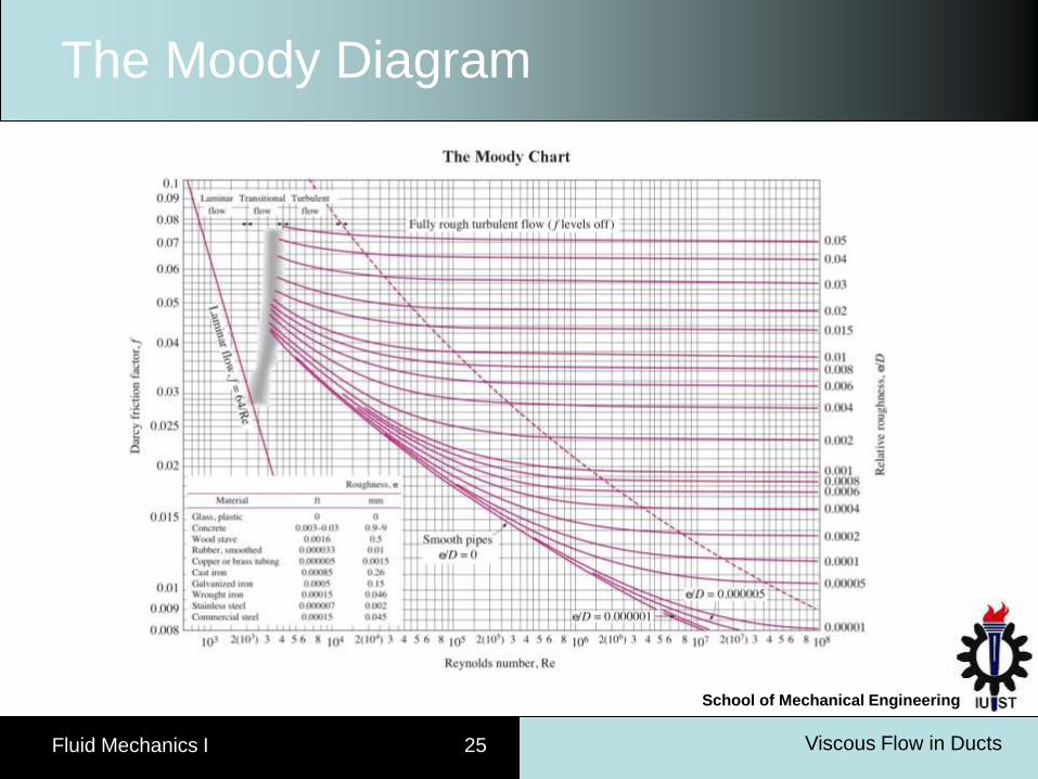
Laminar flow: f = 64/Re (exact)
Turbulent flow: Use charts or empirical equations (Moody Chart, a famous plot of f vs. Re and /D)
But for laminar flow, roughness
does not affect the flow unless it
is huge
4 wf
Lh
g D
2
2f
L Vh f
D g
Viscous Flow in Ducts Fluid Mechanics I 20
School of Mechanical Engineering
Fully Developed Pipe Flow
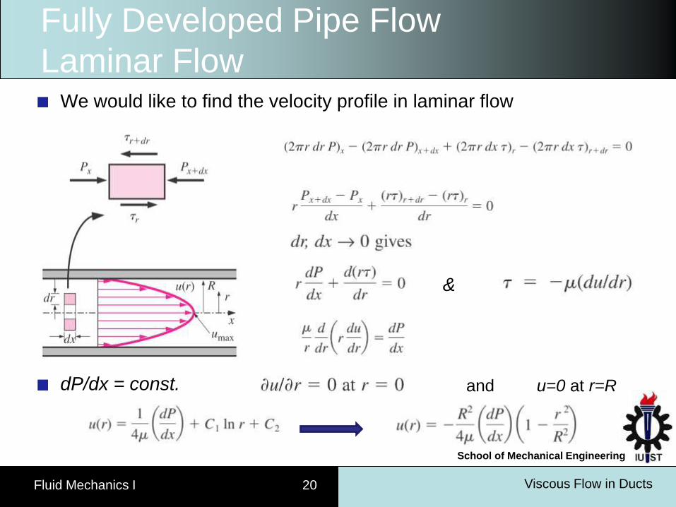
Laminar Flow We would like to find the velocity profile in laminar flow
&
dP/dx = const. and u=0 at r=R
Viscous Flow in Ducts Fluid Mechanics I 21
School of Mechanical Engineering
Fully Developed Pipe Flow
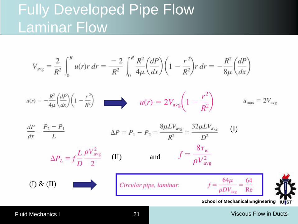
Laminar Flow
(I)
(II) and
(I) & (II)
Viscous Flow in Ducts Fluid Mechanics I 22
School of Mechanical Engineering
Fully Developed Pipe Flow
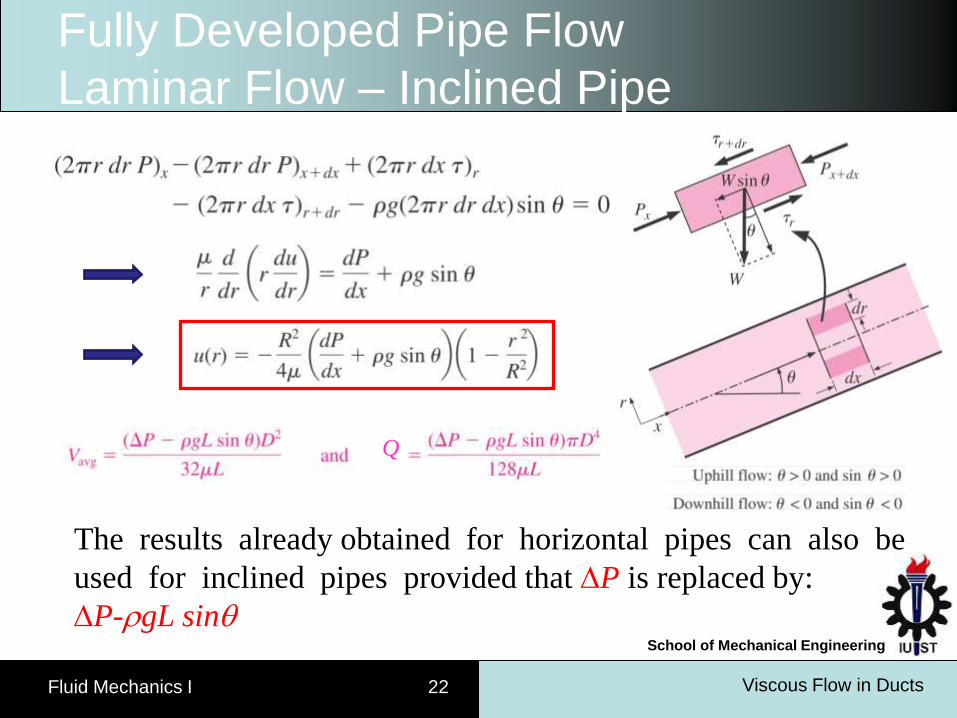
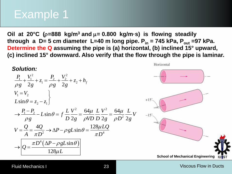
Laminar Flow – Inclined Pipe
The results already obtained for horizontal pipes can also be
used for inclined pipes provided that P is replaced by:
P-gL sin
Q
Viscous Flow in Ducts Fluid Mechanics I 23
School of Mechanical Engineering
Example 1
Oil at 20°C (=888 kg/m3 and = 0.800 kg/m·s) is flowing steadily
through a D= 5 cm diameter L=40 m long pipe. Pin = 745 kPa, Pout =97 kPa.
Determine the Q assuming the pipe is (a) horizontal, (b) inclined 15° upward,
(c) inclined 15° downward. Also verify that the flow through the pipe is laminar.
Solution:
2 2
1 1 2 21 2
1 2
2 1
2 2
1 2
2
2 4
4
2 2
sin
64 64sin
2 2 2
4 128sin
sin
128
f
P V P Vz z h
g g g g
V V
L z z
P P L V L V LL f V
g D g VD D g D g
Q Q LQV P gL
A D D
D P gLQ
L
Viscous Flow in Ducts Fluid Mechanics I 24
School of Mechanical Engineering
Example 1
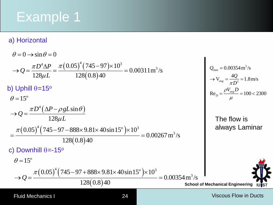
a) Horizontal
4 343
0 sin 0
0.05 745 97 100.00311m /s
128 128 0.8 40
D PQ
L
b) Uphill =15o
o
4
4 o 3
3
15
sin
128
0.05 745 97 888 9.81 40sin15 100.00267m /s
128 0.8 40
D P gLQ
L
c) Downhill =-15o
o
4 o 3
3
15
0.05 745 97 888 9.81 40sin15 100.00354m /s
128 0.8 40Q
3
max
2
0.00354m /s
4V 1.8m/s
Re 100 2300
avg
avg
D
Q
Q
D
V D
The flow is
always Laminar
Viscous Flow in Ducts Fluid Mechanics I 25
School of Mechanical Engineering
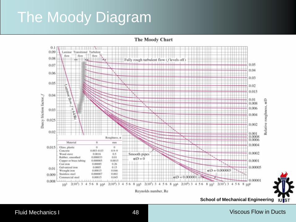
The Moody Diagram
Viscous Flow in Ducts Fluid Mechanics I 26
School of Mechanical Engineering
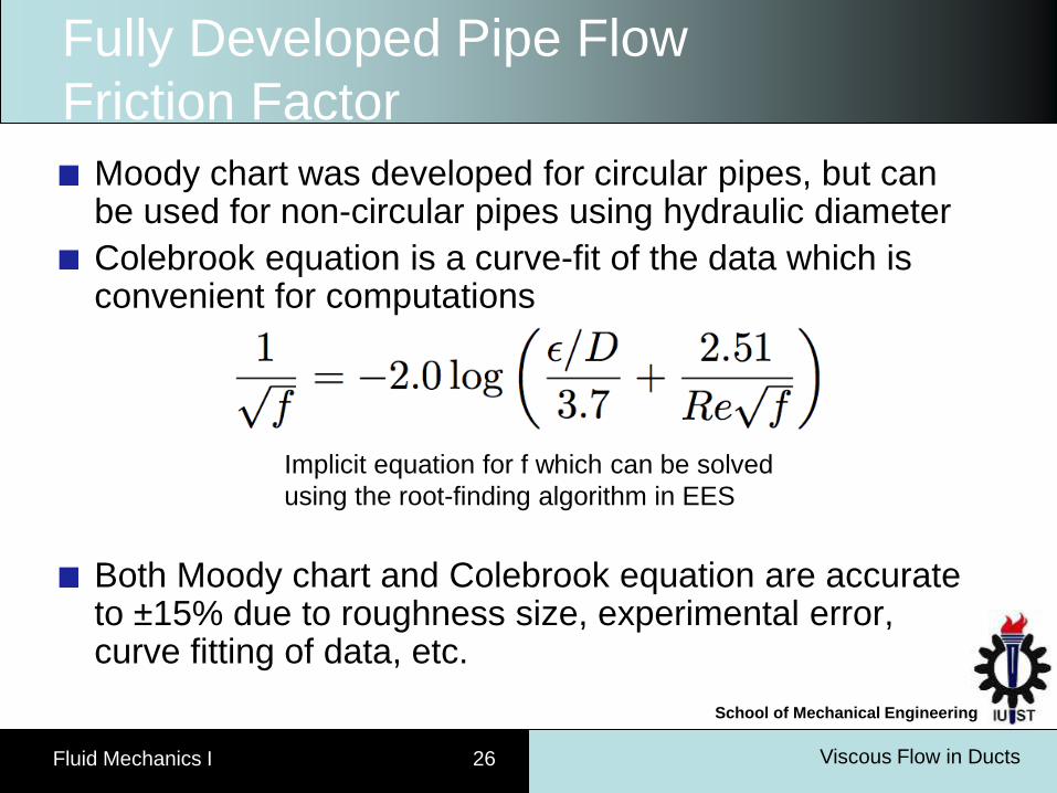
Fully Developed Pipe Flow
Friction Factor
Moody chart was developed for circular pipes, but can be used for non-circular pipes using hydraulic diameter
Colebrook equation is a curve-fit of the data which is convenient for computations
Both Moody chart and Colebrook equation are accurate to ±15% due to roughness size, experimental error, curve fitting of data, etc.
Implicit equation for f which can be solved
using the root-finding algorithm in EES
Viscous Flow in Ducts Fluid Mechanics I 27
School of Mechanical Engineering
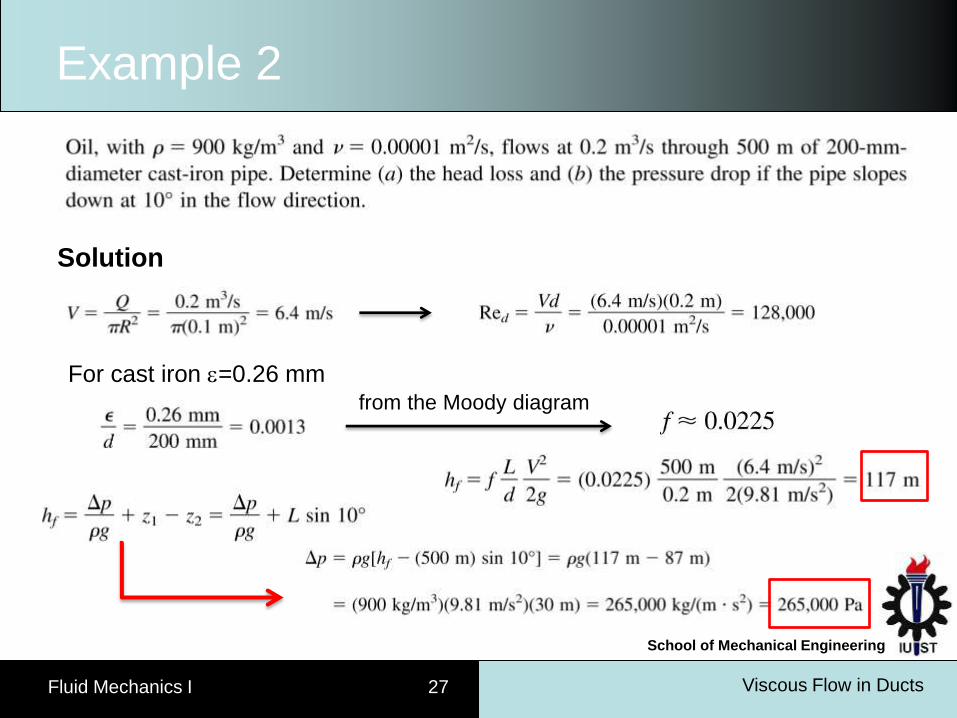
Example 2
Solution
For cast iron =0.26 mm from the Moody diagram
Viscous Flow in Ducts Fluid Mechanics I 28
School of Mechanical Engineering
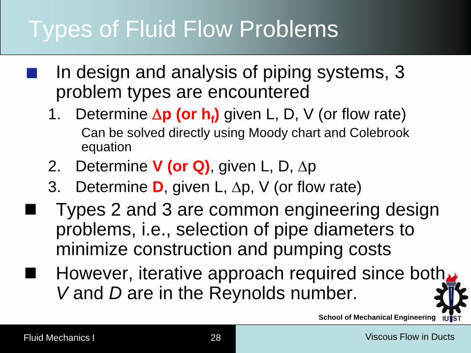
Types of Fluid Flow Problems
In design and analysis of piping systems, 3 problem types are encountered
1. Determine p (or hf) given L, D, V (or flow rate) Can be solved directly using Moody chart and Colebrook equation
2. Determine V (or Q), given L, D, p
3. Determine D, given L, p, V (or flow rate)
Types 2 and 3 are common engineering design problems, i.e., selection of pipe diameters to minimize construction and pumping costs
However, iterative approach required since both V and D are in the Reynolds number.
Viscous Flow in Ducts Fluid Mechanics I 29
School of Mechanical Engineering
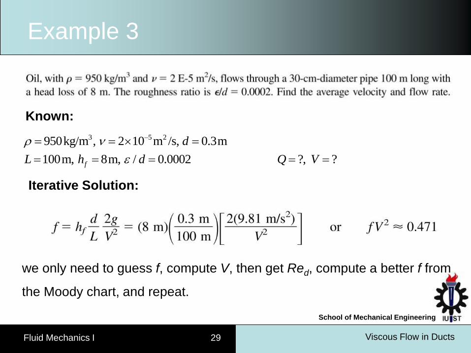
Example 3
Known:
3 5 2950kg/m , 2 10 m /s, 0.3m
100m, 8m, / 0.0002 ?, ?f
d
L h d Q V
we only need to guess f, compute V, then get Red, compute a better f from
the Moody chart, and repeat.
Iterative Solution:
Viscous Flow in Ducts Fluid Mechanics I 30
School of Mechanical Engineering
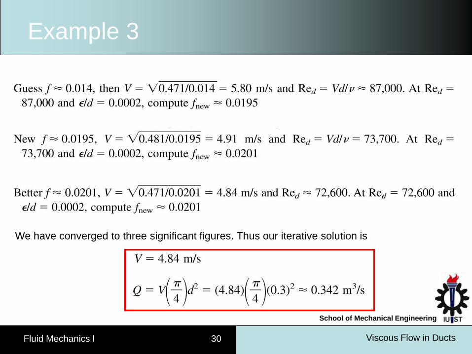
Example 3
We have converged to three significant figures. Thus our iterative solution is
Viscous Flow in Ducts Fluid Mechanics I 31
School of Mechanical Engineering
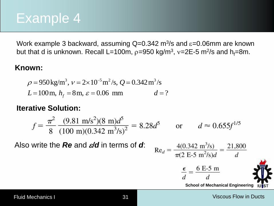
Example 4
Known:
3 5 2 3950kg/m , 2 10 m /s, 0.342m /s
100m, 8m, 0.06 mm ?f
Q
L h d
Also write the Re and /d in terms of d:
Iterative Solution:
Work example 3 backward, assuming Q=0.342 m3/s and =0.06mm are known
but that d is unknown. Recall L=100m, =950 kg/m3, =2E-5 m2/s and hf=8m.
Viscous Flow in Ducts Fluid Mechanics I 32
School of Mechanical Engineering
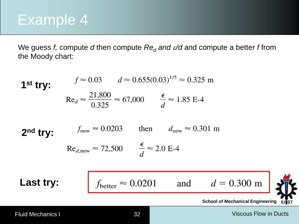
Example 4
We guess f, compute d then compute Red and /d and compute a better f from
the Moody chart:
1st try:
2nd try:
Last try:
Viscous Flow in Ducts Fluid Mechanics I 33
School of Mechanical Engineering
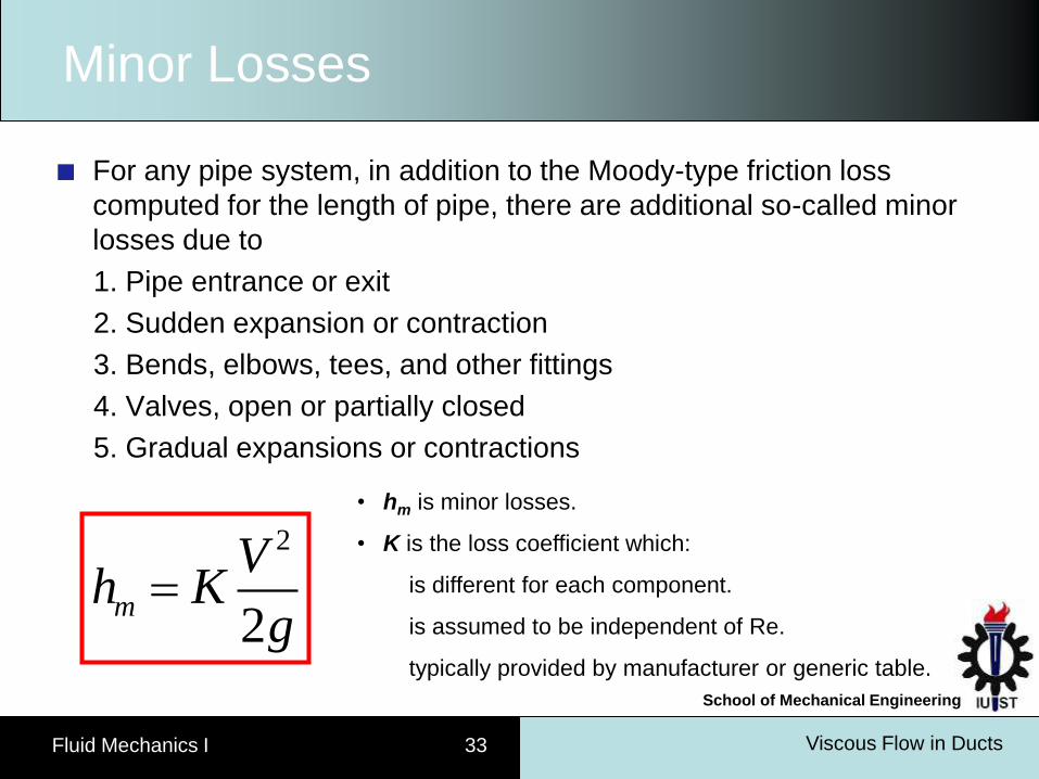
Minor Losses
For any pipe system, in addition to the Moody-type friction loss
computed for the length of pipe, there are additional so-called minor
losses due to
1. Pipe entrance or exit
2. Sudden expansion or contraction
3. Bends, elbows, tees, and other fittings
4. Valves, open or partially closed
5. Gradual expansions or contractions
• hm is minor losses.
• K is the loss coefficient which:
is different for each component.
is assumed to be independent of Re.
typically provided by manufacturer or generic table.
2
2m
Vh K
g
Viscous Flow in Ducts Fluid Mechanics I 34
School of Mechanical Engineering
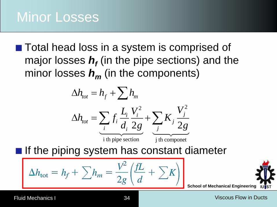
Minor Losses
Total head loss in a system is comprised of
major losses hf (in the pipe sections) and the
minor losses hm (in the components)
If the piping system has constant diameter
22
i th pipe section j th componet
2 2
tot f m
ji itot i j
i ji
h h h
VL Vh f K
d g g
Viscous Flow in Ducts Fluid Mechanics I 35
School of Mechanical Engineering
Minor Losses
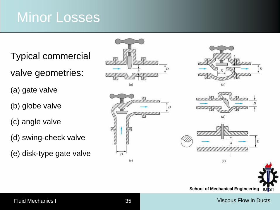
Typical commercial
valve geometries:
(a) gate valve
(b) globe valve
(c) angle valve
(d) swing-check valve
(e) disk-type gate valve
Viscous Flow in Ducts Fluid Mechanics I 36
School of Mechanical Engineering
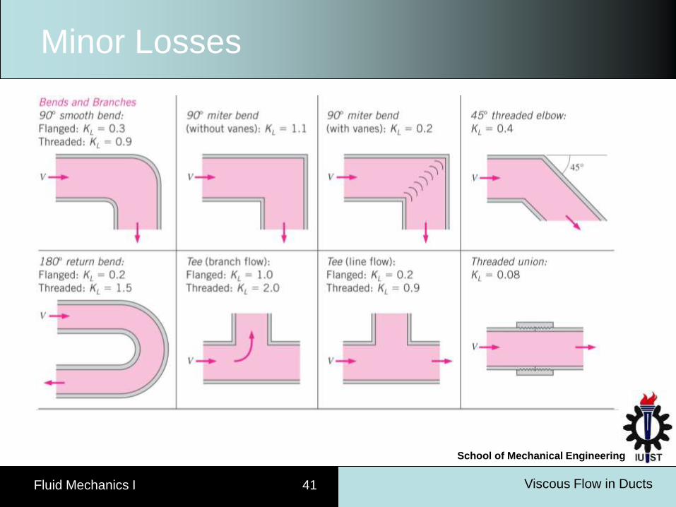
Minor Losses
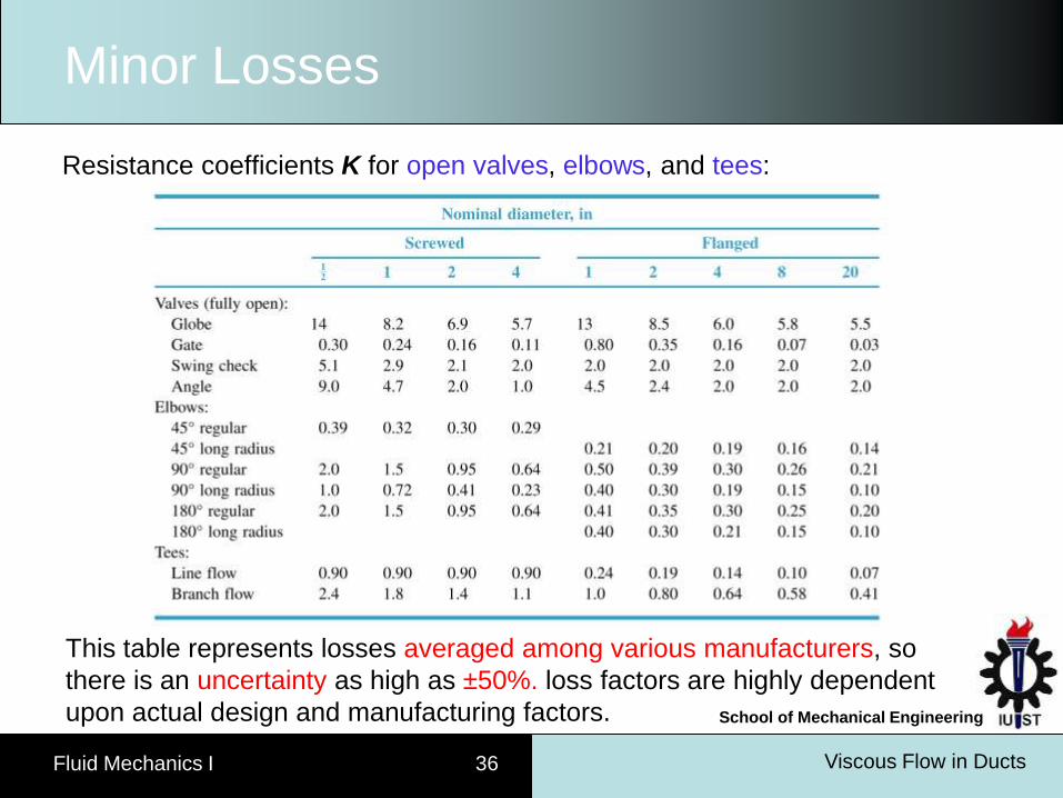
Resistance coefficients K for open valves, elbows, and tees:
This table represents losses averaged among various manufacturers, so
there is an uncertainty as high as ±50%. loss factors are highly dependent
upon actual design and manufacturing factors.
Viscous Flow in Ducts Fluid Mechanics I 37
School of Mechanical Engineering
Minor Losses
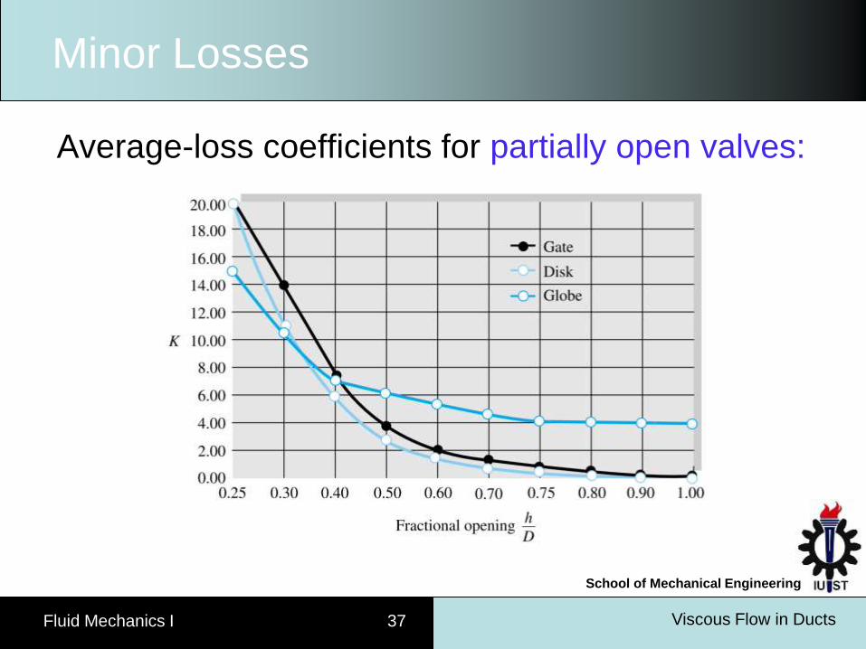
Average-loss coefficients for partially open valves:
Viscous Flow in Ducts Fluid Mechanics I 38
School of Mechanical Engineering
Minor Losses
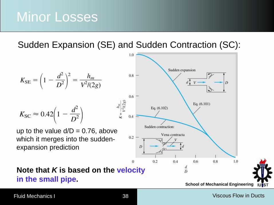
Sudden Expansion (SE) and Sudden Contraction (SC):
Note that K is based on the velocity
in the small pipe.
up to the value d/D = 0.76, above
which it merges into the sudden-
expansion prediction
Viscous Flow in Ducts Fluid Mechanics I 39
School of Mechanical Engineering
Minor Losses
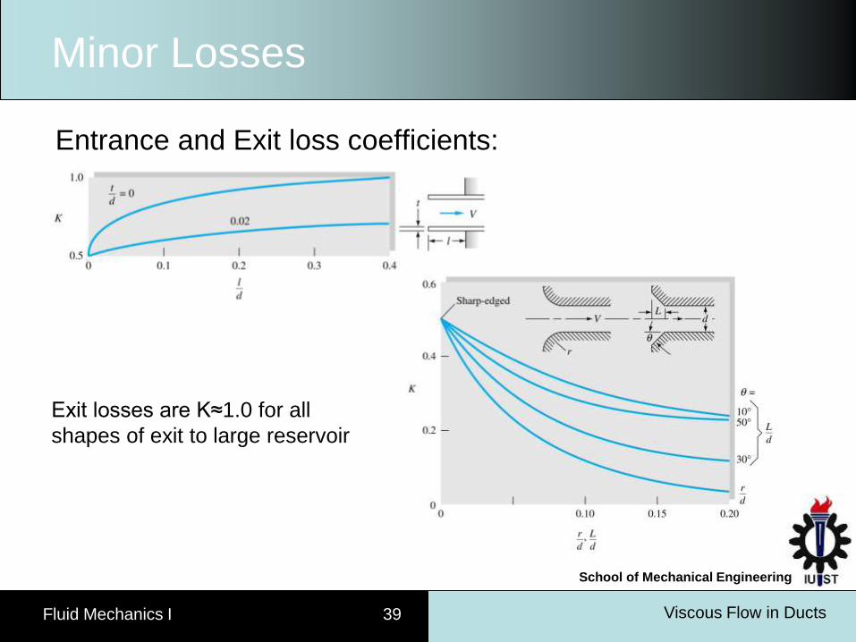
Entrance and Exit loss coefficients:
Exit losses are K≈1.0 for all
shapes of exit to large reservoir
Viscous Flow in Ducts Fluid Mechanics I 40
School of Mechanical Engineering
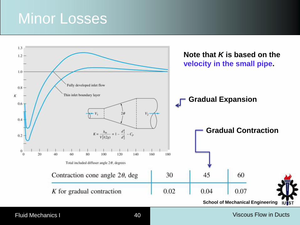
Minor Losses
Note that K is based on the
velocity in the small pipe.
Gradual Expansion
Gradual Contraction
Viscous Flow in Ducts Fluid Mechanics I 41
School of Mechanical Engineering
Minor Losses
Viscous Flow in Ducts Fluid Mechanics I 42
School of Mechanical Engineering
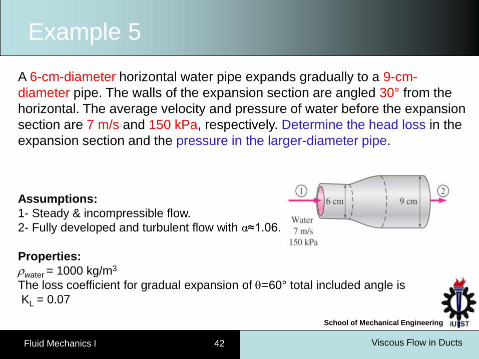
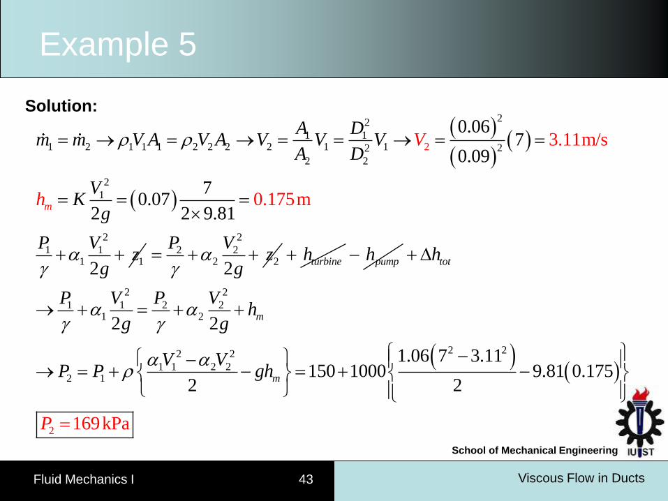
Example 5
A 6-cm-diameter horizontal water pipe expands gradually to a 9-cm-
diameter pipe. The walls of the expansion section are angled 30° from the
horizontal. The average velocity and pressure of water before the expansion
section are 7 m/s and 150 kPa, respectively. Determine the head loss in the
expansion section and the pressure in the larger-diameter pipe.
Assumptions:
1- Steady & incompressible flow.
2- Fully developed and turbulent flow with α≈1.06.
Properties:
water = 1000 kg/m3
The loss coefficient for gradual expansion of =60° total included angle is
KL = 0.07
Viscous Flow in Ducts Fluid Mechanics I 43
School of Mechanical Engineering
Example 5
Solution:
22
1 11 2 1 1 1 2 2 2 2 1 1 22
2 2
2
1
2
1 11
2
1
0.067
0.09
70.07
2 2 9.
3.11m/s
0.175m81
2
m
VA D
m m V A V A V V VA D
VK
g
P Vz
h
g
2
2 22 2
2
P Vz
g
turbineh pumph
2 2
1 1 2 21 2
2 22 2
1 1 2
2
22 1
169k
2 2
1.06 7 3.11150 1000 9.81 0.175
Pa
2 2
tot
m
m
h
P V P Vh
g g
V
P
VP P gh
Viscous Flow in Ducts Fluid Mechanics I 44
School of Mechanical Engineering
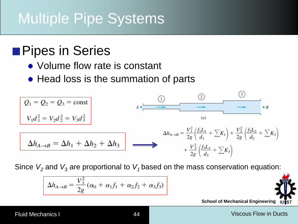
Multiple Pipe Systems
Pipes in Series Volume flow rate is constant
Head loss is the summation of parts
Since V2 and V3 are proportional to V1 based on the mass conservation equation:
Viscous Flow in Ducts Fluid Mechanics I 45
School of Mechanical Engineering
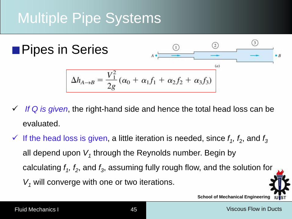
Multiple Pipe Systems
Pipes in Series
If Q is given, the right-hand side and hence the total head loss can be
evaluated.
If the head loss is given, a little iteration is needed, since f1, f2, and f3
all depend upon V1 through the Reynolds number. Begin by
calculating f1, f2, and f3, assuming fully rough flow, and the solution for
V1 will converge with one or two iterations.
Viscous Flow in Ducts Fluid Mechanics I 46
School of Mechanical Engineering
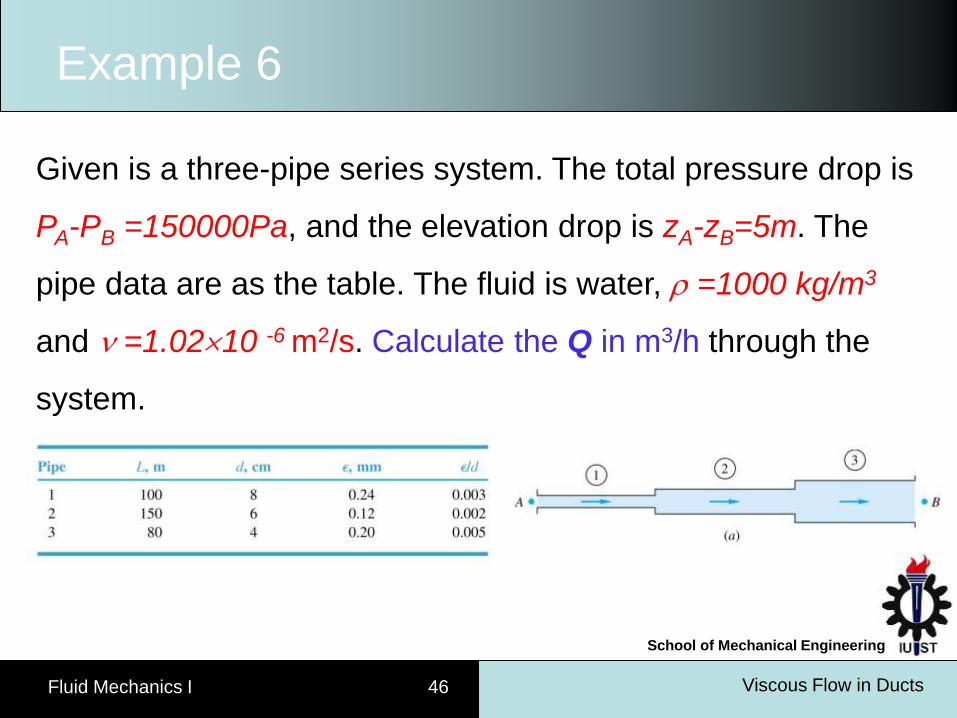
Example 6
Given is a three-pipe series system. The total pressure drop is
PA-PB =150000Pa, and the elevation drop is zA-zB=5m. The
pipe data are as the table. The fluid is water, =1000 kg/m3
and =1.0210 -6 m2/s. Calculate the Q in m3/h through the
system.
Viscous Flow in Ducts Fluid Mechanics I 47
School of Mechanical Engineering
Example 6
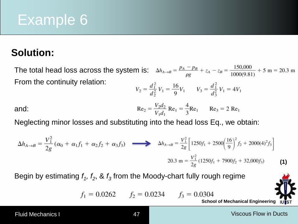
Solution:
The total head loss across the system is:
From the continuity relation:
and:
Neglecting minor losses and substituting into the head loss Eq., we obtain:
Begin by estimating f1, f2, & f3 from the Moody-chart fully rough regime
(1)
Viscous Flow in Ducts Fluid Mechanics I 48
School of Mechanical Engineering
The Moody Diagram
Viscous Flow in Ducts Fluid Mechanics I 49
School of Mechanical Engineering
Example 6
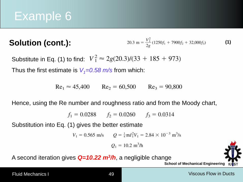
Solution (cont.):
Substitute in Eq. (1) to find:
Thus the first estimate is V1=0.58 m/s from which:
Hence, using the Re number and roughness ratio and from the Moody chart,
Substitution into Eq. (1) gives the better estimate
A second iteration gives Q=10.22 m3/h, a negligible change
(1)
Viscous Flow in Ducts Fluid Mechanics I 50
School of Mechanical Engineering
Multiple Pipe Systems
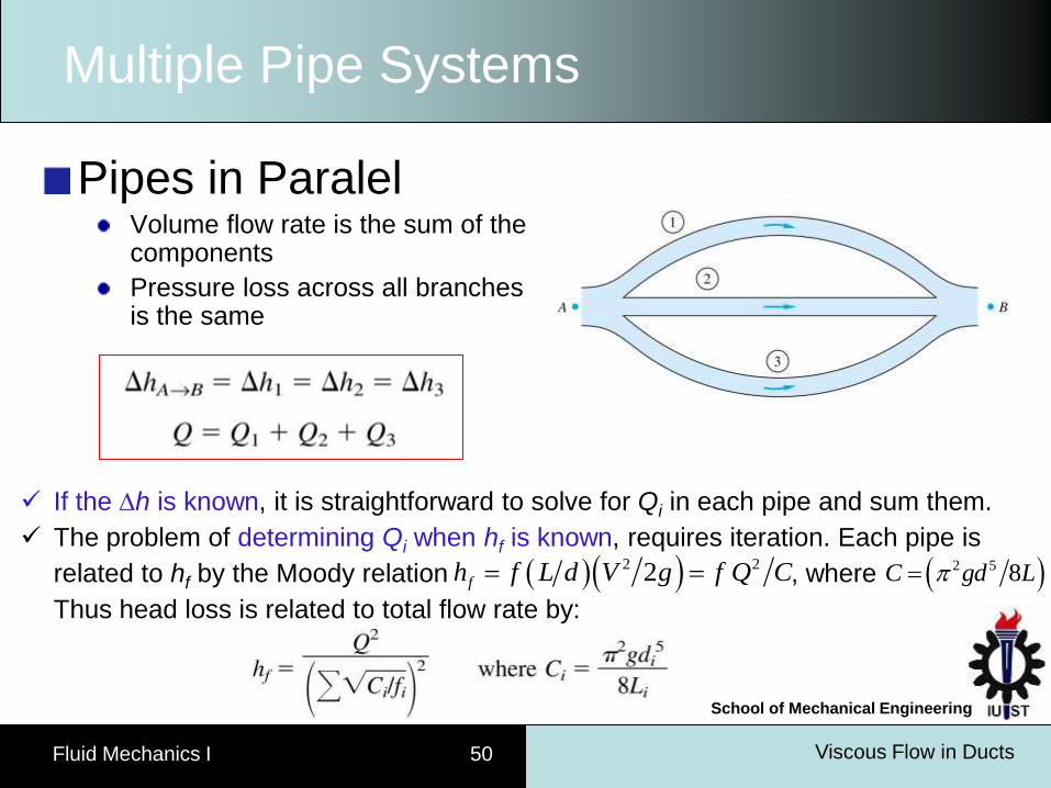
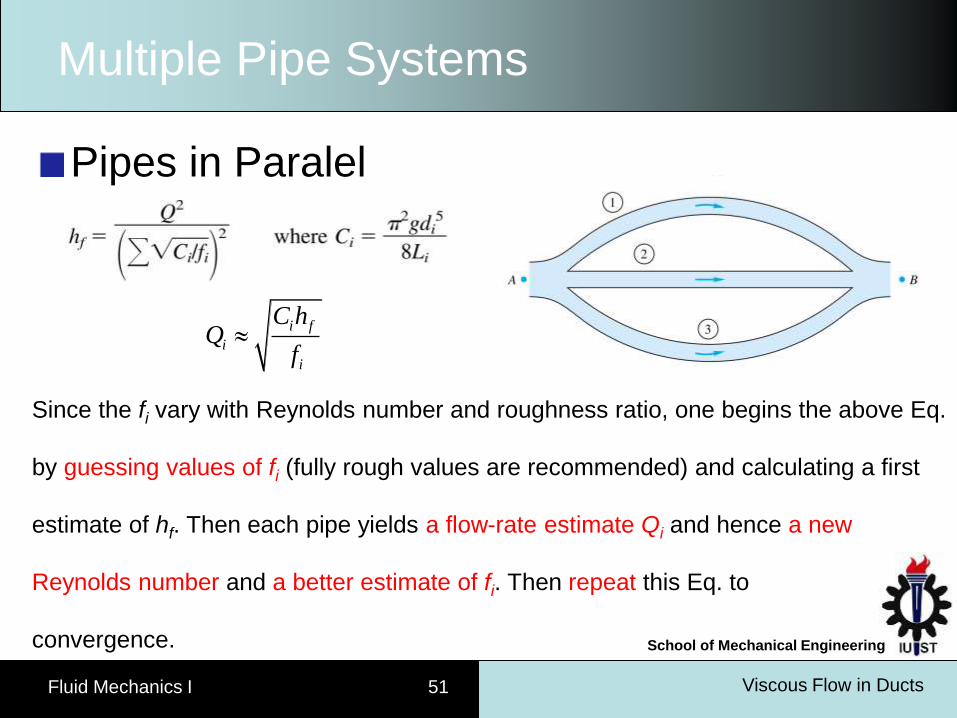
Pipes in Paralel Volume flow rate is the sum of the components
Pressure loss across all branches is the same
If the h is known, it is straightforward to solve for Qi in each pipe and sum them.
The problem of determining Qi when hf is known, requires iteration. Each pipe is
related to hf by the Moody relation , where
Thus head loss is related to total flow rate by:
2 5 8C gd L 2 22fh f L d V g f Q C
Viscous Flow in Ducts Fluid Mechanics I 51
School of Mechanical Engineering
Multiple Pipe Systems
Pipes in Paralel
Since the fi vary with Reynolds number and roughness ratio, one begins the above Eq.
by guessing values of fi (fully rough values are recommended) and calculating a first
estimate of hf. Then each pipe yields a flow-rate estimate Qi and hence a new
Reynolds number and a better estimate of fi. Then repeat this Eq. to
convergence.
i f
i
i
C hQ
f
Viscous Flow in Ducts Fluid Mechanics I 52
School of Mechanical Engineering
Example 7
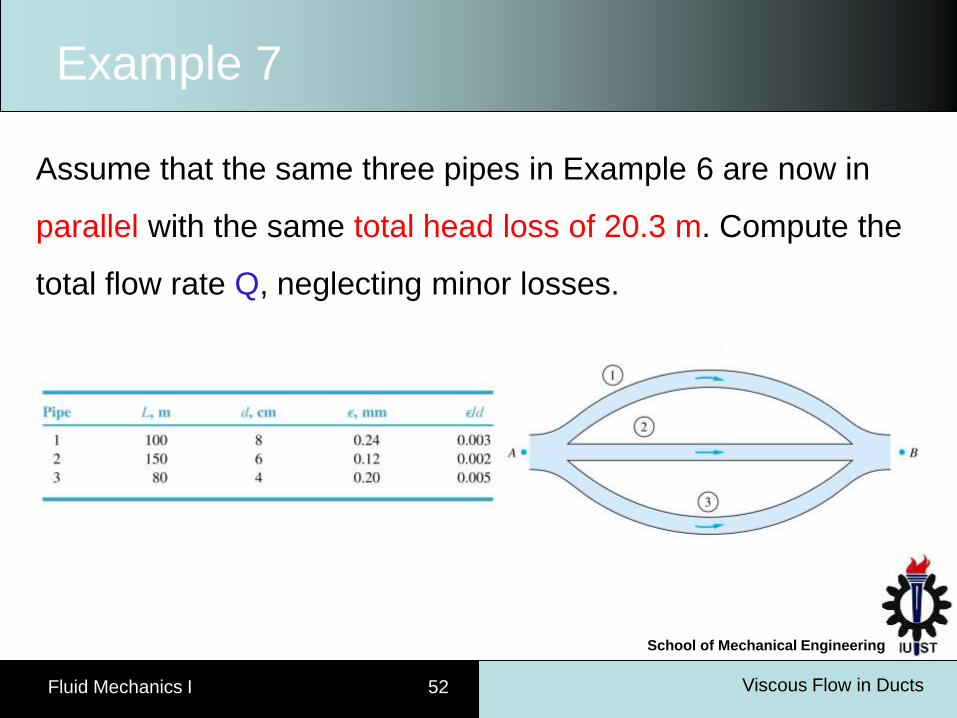
Assume that the same three pipes in Example 6 are now in
parallel with the same total head loss of 20.3 m. Compute the
total flow rate Q, neglecting minor losses.
Viscous Flow in Ducts Fluid Mechanics I 53
School of Mechanical Engineering
Example 7
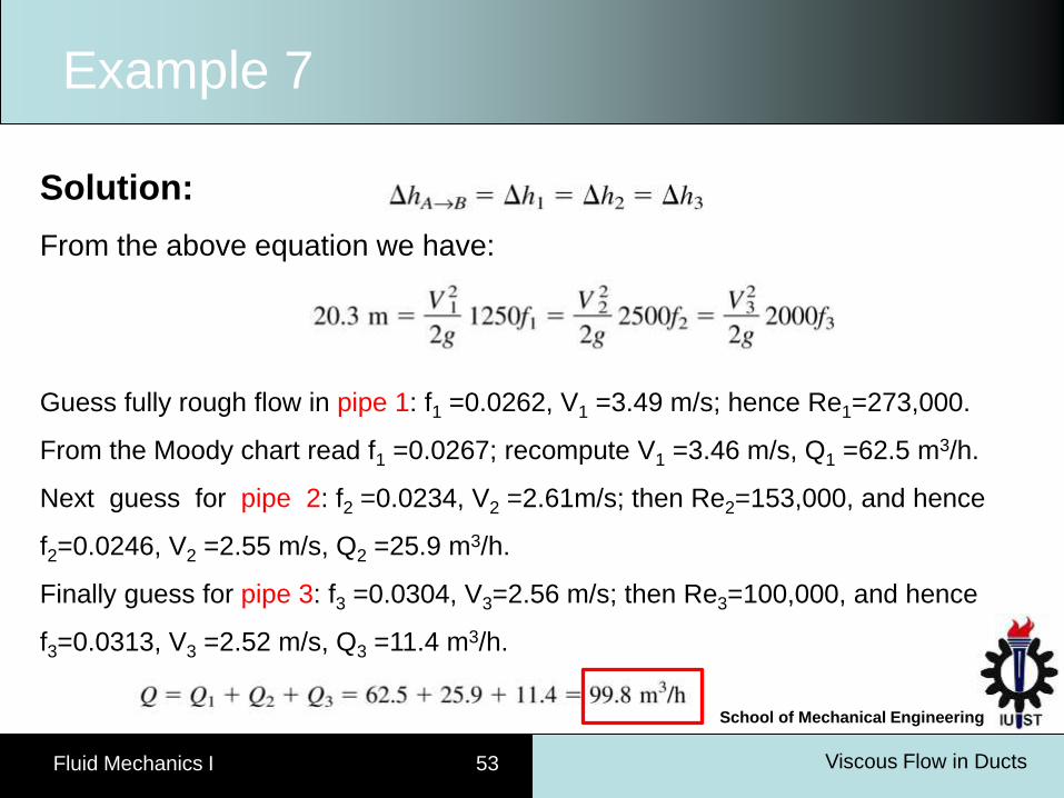
Solution:
From the above equation we have:
Guess fully rough flow in pipe 1: f1 =0.0262, V1 =3.49 m/s; hence Re1=273,000.
From the Moody chart read f1 =0.0267; recompute V1 =3.46 m/s, Q1 =62.5 m3/h.
Next guess for pipe 2: f2 =0.0234, V2 =2.61m/s; then Re2=153,000, and hence
f2=0.0246, V2 =2.55 m/s, Q2 =25.9 m3/h.
Finally guess for pipe 3: f3 =0.0304, V3=2.56 m/s; then Re3=100,000, and hence
f3=0.0313, V3 =2.52 m/s, Q3 =11.4 m3/h.
Viscous Flow in Ducts Fluid Mechanics I 54
School of Mechanical Engineering
Multiple Pipe Systems
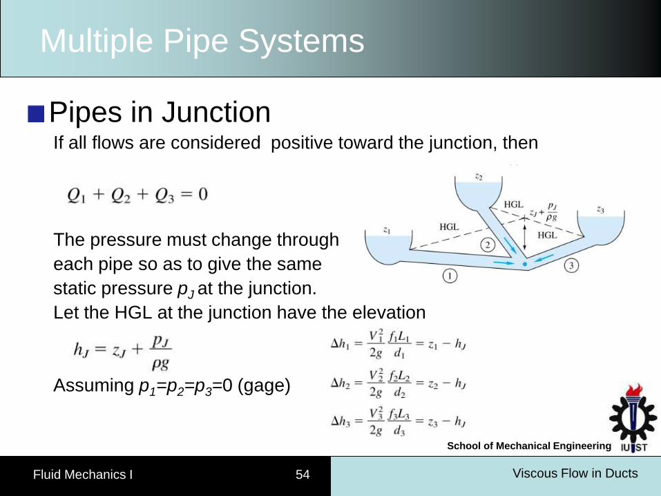
Pipes in Junction If all flows are considered positive toward the junction, then
The pressure must change through
each pipe so as to give the same
static pressure pJ at the junction.
Let the HGL at the junction have the elevation
Assuming p1=p2=p3=0 (gage)
Viscous Flow in Ducts Fluid Mechanics I 55
School of Mechanical Engineering
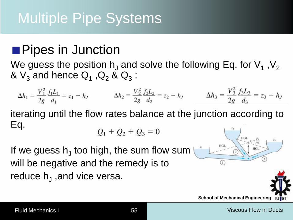
Multiple Pipe Systems
Pipes in Junction We guess the position hJ and solve the following Eq. for V1 ,V2 & V3 and hence Q1 ,Q2 & Q3 :
iterating until the flow rates balance at the junction according to Eq.
If we guess hJ too high, the sum flow sum
will be negative and the remedy is to
reduce hJ ,and vice versa.
Viscous Flow in Ducts Fluid Mechanics I 56
School of Mechanical Engineering
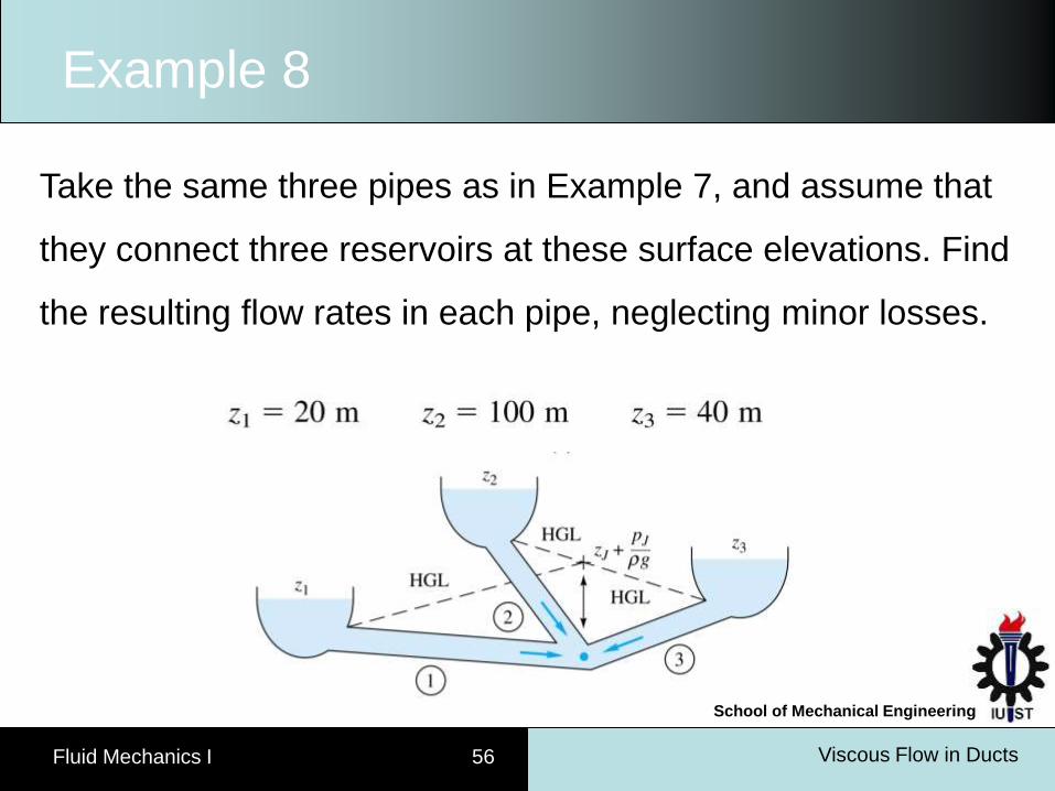
Example 8
Take the same three pipes as in Example 7, and assume that
they connect three reservoirs at these surface elevations. Find
the resulting flow rates in each pipe, neglecting minor losses.
Viscous Flow in Ducts Fluid Mechanics I 57
School of Mechanical Engineering
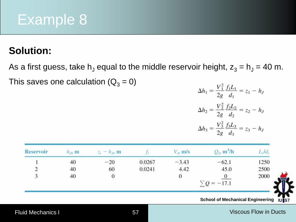
Example 8
Solution:
As a first guess, take hJ equal to the middle reservoir height, z3 = hJ = 40 m.
This saves one calculation (Q3 = 0)
Viscous Flow in Ducts Fluid Mechanics I 58
School of Mechanical Engineering
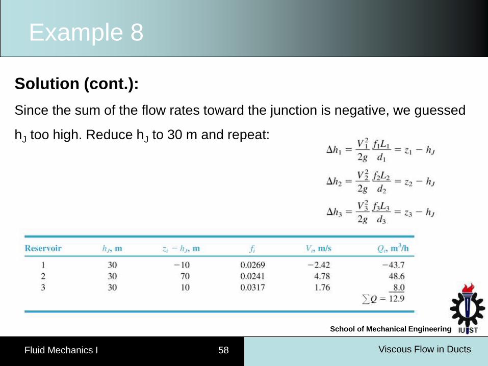
Example 8
Solution (cont.):
Since the sum of the flow rates toward the junction is negative, we guessed
hJ too high. Reduce hJ to 30 m and repeat:
Viscous Flow in Ducts Fluid Mechanics I 59
School of Mechanical Engineering
Example 8
Solution (cont.):
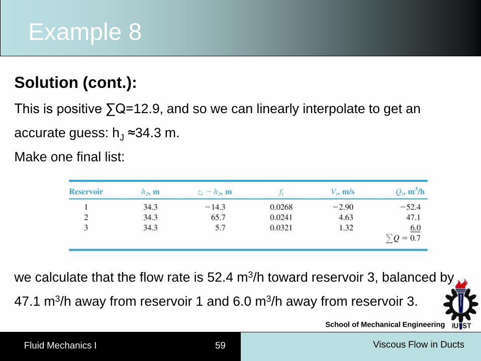
This is positive ∑Q=12.9, and so we can linearly interpolate to get an
accurate guess: hJ ≈34.3 m.
Make one final list:
we calculate that the flow rate is 52.4 m3/h toward reservoir 3, balanced by
47.1 m3/h away from reservoir 1 and 6.0 m3/h away from reservoir 3.
Viscous Flow in Ducts Fluid Mechanics I 60
School of Mechanical Engineering
Multiple Pipe Systems
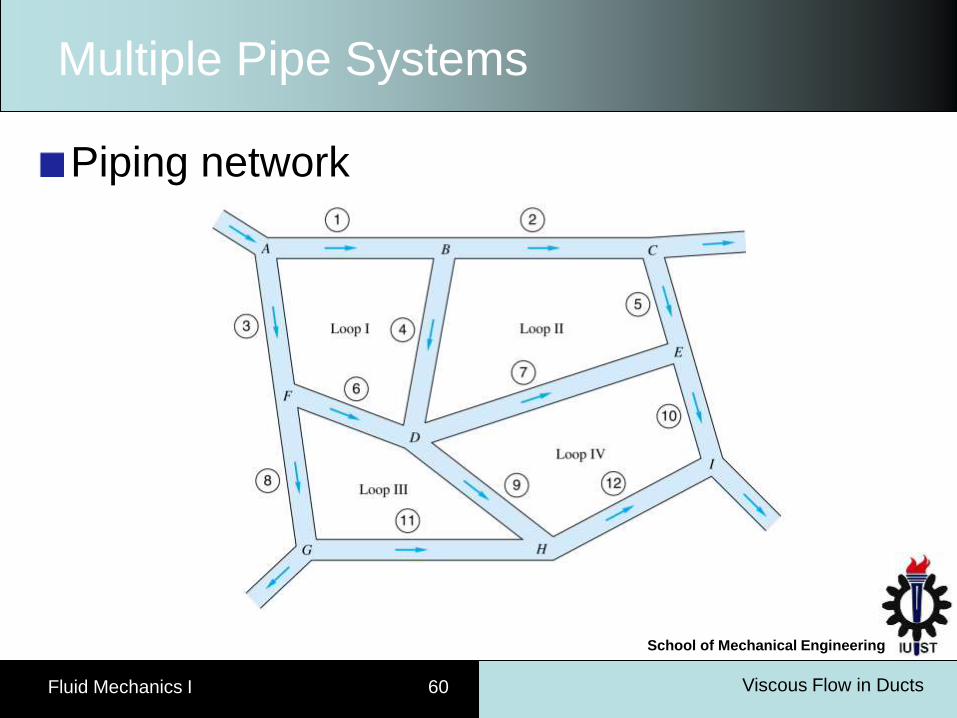
Piping network
Viscous Flow in Ducts Fluid Mechanics I 61
School of Mechanical Engineering
Multiple Pipe Systems
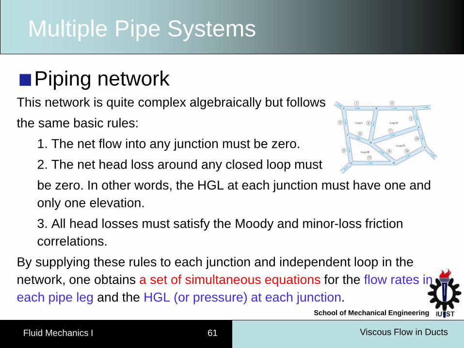
Piping network This network is quite complex algebraically but follows
the same basic rules:
1. The net flow into any junction must be zero.
2. The net head loss around any closed loop must
be zero. In other words, the HGL at each junction must have one and
only one elevation.
3. All head losses must satisfy the Moody and minor-loss friction
correlations.
By supplying these rules to each junction and independent loop in the
network, one obtains a set of simultaneous equations for the flow rates in
each pipe leg and the HGL (or pressure) at each junction.


![Viscous Flow Ch8[1]](https://static.fdocuments.net/doc/165x107/577ccd371a28ab9e788bce8d/viscous-flow-ch81.jpg)