
Viscothermal wave propagation including acousto-elastic ... · VISCOTHERMAL WAVE PROPAGATION...
218
Viscothermal wave propagation including acousto-elastic interaction W.M. Beltman
Transcript of Viscothermal wave propagation including acousto-elastic ... · VISCOTHERMAL WAVE PROPAGATION...

Viscothermal wave propagationincluding acousto-elastic interaction
W.M. Beltman

CIP-DATA KONINKLIJKE BIBLIOTHEEK, DEN HAAG
Beltman, Willem Marinus
Viscothermal wave propagation including acousto-elastic interaction /Beltman, Willem Marinus. [S.1 : s.n.]. -Ill.Thesis Enschede.- With ref. - With summary in Dutch.ISBN 90-3651217-4
Subject headings: acoustics, acousto-elasticity, viscothermal wavepropagation, finite elements
Cover: Laserium “Pink Floyd - The Wall”(We don’t need no education...) at the GriffithObservatory, Hollywood, California on February 8,1998. Artist: Tim Barrett. Picture: Marco Beltman.With permission of Laser Images Inc. and theGriffith Observatory.
Copyright c©1998 by W.M. Beltman, Enschede

VISCOTHERMAL WAVE PROPAGATIONINCLUDING ACOUSTO-ELASTIC INTERACTION
PROEFSCHRIFT
ter verkrijging vande graad van doctor aan de Universiteit Twente,
op gezag van de rector magnificus,prof.dr. F.A. van Vught,
volgens besluit van het College voor Promotiesin het openbaar te verdedigen
op donderdag 22 oktober 1998 te 15:00 uur
door
Willem Marinus Beltman
geboren op 19 juli 1971
te Gorssel

DIT PROEFSCHRIFT IS GOEDGEKEURD DOOR:
PROMOTOR: PROF.DR.IR. H. TIJDEMAN
Preface
Completing this work would not have been possible without the support andco-operation of a large number of people. First of all I thank my supervisor,Henk Tijdeman, for giving me the opportunity to carry out this research.He is always ready to offer support to his students and has created a verypleasant working environment with good facilities. I enjoyed working in thedynamics group with my colleagues Ruud Spiering, Peter van der Hoogt,Bert Wolbert, Frits van der Eerden and Tom Basten. I am indebted toDebbie Vrieze and Piet Laan for their administrative and computer supportrespectively.
A number of MSc students performed their graduation research withinthe framework of my thesis project. Their work made very important con-tributions to the present study. I thank all students for their work and thepleasant time.
This project was carried out in close co-operation with, and supportedby, a number of firms and institutions. The co-operation was very enjoyableand the industrial application of the newly developed techniques added anextra dimension to my work. I thank Frank Grooteman, Andre de Boer(National Aerospace Laboratory), Berend Winter, Marcel Ellenbroek, JaapWijker (Fokker Space), Rob Dokter, Freek van Beek, Pieter van Groos (OceTechnologies), Bert Roozen (Philips Research Laboratories), Charles van deVen, Gerard Westendorp (Nefit Fasto). The financial support from Shell andthe Technology Foundation is gratefully acknowledged.
Kees Venner, and Ysbrand Wijnant contributed with valuable sugges-tions, help and comments. I thank Bart Paarhuis and Katrina Emmett fortheir help in improving the manuscript.

vi
Finally, I thank my family and friends for all their support. My parentshave always stimulated and encouraged my brother, my sister and myself inour efforts, often making sacrifices for our sake. They deserve a big compli-ment.
Thank you,
Enschede, 22 October 1998
Marco Beltman

Summary
This research deals with pressure waves in a gas trapped in thin layers ornarrow tubes. In these cases viscous and thermal effects can have a significanteffect on the propagation of waves. This so-called viscothermal wave propa-gation is governed by a number of dimensionless parameters. The two mostimportant parameters are the shear wave number and the reduced frequency.These parameters were used to put into perspective the models that werepresented in the literature. The analysis shows that the complete parame-ter range is covered by three classes of models: the standard wave equationmodel, the low reduced frequency model and the full linearized Navier Stokesmodel. For the majority of practical situations the low reduced frequencymodel is sufficient and the most efficient to describe viscothermal wave propa-gation. The full linearized Navier Stokes model should only be used underextreme conditions. The low reduced frequency model was experimentallyvalidated with a specially designed large-scale setup. A light and stiff solarpanel, located parallel to a fixed surface and performing a small amplitudenormal oscillation, was used. By assuming the panel to be rigid, attentioncould be focused on the viscothermal model. The large scale of the setup en-abled accurate measurements and detailed information to be obtained aboutthe pressure distribution in the layer. Analytical and experimental resultsshow good agreement: the low reduced frequency model is very well suitedto describe viscothermal wave propagation. In practical applications thesurfaces or walls are often flexible and there can be a strong interaction be-tween the wave propagation and surface or wall motion. As a next step,a new viscothermal finite element was developed, based on the low reducedfrequency model. The new element can be coupled to structural elements, en-abling fully coupled acousto-elastic calculations for complex geometries. Theacousto-elastic model was experimentally validated for a flexible plate backedby a thin air layer. The results show that the viscothermal effects lead to asignificant energy dissipation in the layer. Furthermore, the acousto-elasticcoupling was essential and had to be included in the analysis. Numericaland experimental results show good agreement: a new reliable viscothermal

viii
acousto-elastic simulation tool has been developed. An additional series ofpreliminary measurements indicate that obstructions in a layer may furtherincrease the energy dissipation. However, non-linear behaviour was observedthat could not be described with the linear viscothermal models. A simplemodel was developed that explained the non-linear behaviour. Finally, thedeveloped techniques were successfully applied to a number of problems: thebehaviour of stacked solar panels attached to a satellite during launch, thedesign of a new inkjet print head and the acoustic behaviour of double wallpanels.

Samenvatting
Dit onderzoek richt zich op het beschrijven van drukgolven die zich voort-planten in een dunne laag gas of in een gas dat zich bevindt in een nauwebuis. In deze gevallen kunnen viskeuze en thermische effecten een belang-rijke invloed hebben op de voortplanting van deze golven. Het gedrag wordtbepaald door een aantal dimensieloze kentallen. De twee belangrijkste ken-tallen zijn het “shear wave” getal en de gereduceerde frequentie. Met dezeparameters zijn de modellen die in de literatuur gepresenteerd zijn in per-spectief geplaatst. De analyse toont aan dat het volledige parameterge-bied bestreken wordt door drie klassen modellen: het standaard golfvergelij-kingsmodel, het lage gereduceerde frequentie model en het volledige geli-neariseerde Navier Stokes model. Voor nagenoeg alle praktische situatiesis het lage gereduceerde frequentie model voldoende en het meest efficientom golfvoortplanting inclusief viskeuze en thermische effecten te beschrijven.Het volledige gelineariseerde Navier Stokes model hoeft alleen onder zeerextreme omstandigheden gebruikt te worden. Het lage gereduceerde fre-quentie model is experimenteel gevalideerd aan de hand van een speciaalontworpen testopstelling. Hiervoor is een licht en stijf zonnepaneel gebruiktdat zich parallel aan een vaste wand bevindt. Het paneel voert een trillingmet een kleine amplitude uit loodrecht op de wand. Doordat het paneelzich star gedraagt kan alle aandacht gericht worden op het golfvoortplan-tingsmodel. De grote afmetingen van de opstelling maken metingen met eenhoge mate van nauwkeurigheid mogelijk en bovendien is gedetailleerde infor-matie verkregen over de drukverdeling in de luchtspleet tussen paneel en vastoppervlak. Analytische en experimentele resultaten komen goed overeen: hetlage gereduceerde frequentie model is erg geschikt om golfvoortplanting in-clusief viskeuze en thermische effecten te beschrijven. In de praktijk heeftmen vaak te maken met flexibele oppervlakken of wanden. Er kan een sterkeinteractie zijn tussen de golfvoortplanting en de elastische wandbeweging. Alsvervolg is daarom een nieuw akoestisch eindig element ontwikkeld, gebaseerdop het lage gereduceerde frequentie model. Dit element is in staat omgolfvoortplanting inclusief thermische en viskeuze effecten te beschrijven. Het

x
kan gekoppeld worden aan constructie elementen, waardoor volledig gekop-pelde berekeningen voor complexe geometrieen mogelijk zijn. Het akoesto-elastische eindige elementen model is gevalideerd aan de hand van experi-menten met een ingeklemde plaat met daaronder een dunne luchtlaag. Deresultaten laten zien dat een aanzienlijke hoeveelheid energie gedissipeerdkan worden door viskeuze effecten. Daarnaast is de koppeling erg belangrijk.De numerieke en experimentele resultaten vertonen goede overeenkomst: eris een nieuwe en betrouwbare berekeningsmethode ontwikkeld voor akoesto-elastische problemen, inclusief viskeuze en thermische effecten. Orienterendemetingen tonen aan dat obstructies in een dunne laag de energiedissipatieverder kunnen doen toenemen. Dit gedrag is echter sterk niet-lineair vankarakter en kan derhalve niet voorspeld worden met de lineaire modellen. Eris een eenvoudig model ontwikkeld dat het niet-lineaire gedrag verklaart. Deontwikkelde technieken zijn tenslotte succesvol ingezet bij een aantal prakti-sche toepassingen: het gedrag van opgevouwen zonnepanelen aan een satelliettijdens de lancering, het ontwerp van een inkjet printkop en het akoestischgedrag van dubbelwandige panelen.
Contents
Preface v
Summary vii
Samenvatting ix
Contents xi
1 Introduction 11.1 General introduction . . . . . . . . . . . . . . . . . . . . . . . 1
1.1.1 Acoustics . . . . . . . . . . . . . . . . . . . . . . . . . 11.1.2 Standard acoustic wave propagation . . . . . . . . . . . 21.1.3 Solution techniques for standard acoustic wave propa-
gation . . . . . . . . . . . . . . . . . . . . . . . . . . . 31.1.4 Viscothermal wave propagation . . . . . . . . . . . . . 41.1.5 Solution techniques for viscothermal wave propagation 51.1.6 Acousto-elasticity . . . . . . . . . . . . . . . . . . . . . 51.1.7 Solution techniques for acousto-elastic problems . . . . 61.1.8 Applications . . . . . . . . . . . . . . . . . . . . . . . . 6
1.2 Formulation of the problem . . . . . . . . . . . . . . . . . . . 61.3 Outline . . . . . . . . . . . . . . . . . . . . . . . . . . . . . . . 6
2 Linear viscothermal wave propagation 92.1 Introduction . . . . . . . . . . . . . . . . . . . . . . . . . . . . 92.2 Basic equations . . . . . . . . . . . . . . . . . . . . . . . . . . 11
2.2.1 Derivation of equations . . . . . . . . . . . . . . . . . . 112.2.2 Boundary conditions . . . . . . . . . . . . . . . . . . . 132.2.3 Geometries and co-ordinate systems . . . . . . . . . . . 14
2.3 Full linearized Navier Stokes model . . . . . . . . . . . . . . . 152.3.1 Derivation of equations . . . . . . . . . . . . . . . . . . 152.3.2 Solution strategy . . . . . . . . . . . . . . . . . . . . . 16

xii CONTENTS
2.3.3 Acoustic and entropic wave numbers . . . . . . . . . . 172.3.4 Acousto-elastic coupling . . . . . . . . . . . . . . . . . 182.3.5 Literature . . . . . . . . . . . . . . . . . . . . . . . . . 19
2.4 Simplified Navier Stokes models . . . . . . . . . . . . . . . . . 212.4.1 Trochidis model . . . . . . . . . . . . . . . . . . . . . . 212.4.2 Moser model . . . . . . . . . . . . . . . . . . . . . . . 222.4.3 Acousto-elastic coupling . . . . . . . . . . . . . . . . . 232.4.4 Literature . . . . . . . . . . . . . . . . . . . . . . . . . 23
2.5 Low reduced frequency model . . . . . . . . . . . . . . . . . . 252.5.1 Derivation of equations . . . . . . . . . . . . . . . . . . 252.5.2 Solution strategy . . . . . . . . . . . . . . . . . . . . . 262.5.3 Physical interpretation . . . . . . . . . . . . . . . . . . 282.5.4 Acousto-elastic coupling . . . . . . . . . . . . . . . . . 292.5.5 Literature . . . . . . . . . . . . . . . . . . . . . . . . . 30
2.6 Dimensionless parameters . . . . . . . . . . . . . . . . . . . . 322.6.1 Validity of models . . . . . . . . . . . . . . . . . . . . . 322.6.2 Practical implications . . . . . . . . . . . . . . . . . . . 332.6.3 Overview of the literature for layers . . . . . . . . . . . 35
2.7 Conclusions . . . . . . . . . . . . . . . . . . . . . . . . . . . . 36
3 Fundamental solutions 373.1 Introduction . . . . . . . . . . . . . . . . . . . . . . . . . . . . 373.2 Spherical resonator . . . . . . . . . . . . . . . . . . . . . . . . 38
3.2.1 Introduction . . . . . . . . . . . . . . . . . . . . . . . . 383.2.2 Basic equations . . . . . . . . . . . . . . . . . . . . . . 393.2.3 Solution of the scalar wave equations . . . . . . . . . . 393.2.4 Solution of the vector wave equation . . . . . . . . . . 403.2.5 Rigid sphere with isothermal walls . . . . . . . . . . . 403.2.6 Model extensions . . . . . . . . . . . . . . . . . . . . . 413.2.7 Example: eigenfrequencies of spherical resonator . . . . 41
3.3 Circular tubes . . . . . . . . . . . . . . . . . . . . . . . . . . . 433.3.1 Introduction . . . . . . . . . . . . . . . . . . . . . . . . 433.3.2 Full linearized Navier Stokes model . . . . . . . . . . . 433.3.3 Low reduced frequency model . . . . . . . . . . . . . . 453.3.4 Example: propagation constant . . . . . . . . . . . . . 46
3.4 Miniaturized transducer . . . . . . . . . . . . . . . . . . . . . 503.4.1 Full linearized Navier Stokes solution . . . . . . . . . . 503.4.2 Low reduced frequency solution . . . . . . . . . . . . . 533.4.3 Example: membrane impedance . . . . . . . . . . . . . 53
3.5 Squeeze film damping between plates . . . . . . . . . . . . . . 553.5.1 Simplified Navier Stokes solution . . . . . . . . . . . . 56

CONTENTS xiii
3.5.2 Low reduced frequency solution . . . . . . . . . . . . . 573.5.3 Example: loss factor . . . . . . . . . . . . . . . . . . . 57
4 The low reduced frequency model 594.1 Introduction . . . . . . . . . . . . . . . . . . . . . . . . . . . . 594.2 Analytical calculations . . . . . . . . . . . . . . . . . . . . . . 61
4.2.1 Pressure distribution . . . . . . . . . . . . . . . . . . . 614.2.2 Mobility function . . . . . . . . . . . . . . . . . . . . . 624.2.3 Physical interpretation . . . . . . . . . . . . . . . . . . 63
4.3 Standard acoustic finite element calculations . . . . . . . . . . 654.4 Experiments . . . . . . . . . . . . . . . . . . . . . . . . . . . . 66
4.4.1 Experimental setup . . . . . . . . . . . . . . . . . . . . 664.4.2 Dimensionless parameters . . . . . . . . . . . . . . . . 684.4.3 Validation of the measurement procedure . . . . . . . . 694.4.4 Accuracy of the measurements . . . . . . . . . . . . . . 694.4.5 Experimental results . . . . . . . . . . . . . . . . . . . 72
4.5 Comparison between theory and experiments . . . . . . . . . . 734.5.1 Eigenfrequency . . . . . . . . . . . . . . . . . . . . . . 734.5.2 Damping coefficient . . . . . . . . . . . . . . . . . . . . 734.5.3 Pressure . . . . . . . . . . . . . . . . . . . . . . . . . . 75
4.6 Panel rotating around central axis . . . . . . . . . . . . . . . . 784.6.1 Analytical calculations . . . . . . . . . . . . . . . . . . 784.6.2 Experiments . . . . . . . . . . . . . . . . . . . . . . . . 794.6.3 Comparison between theory and experiments . . . . . . 80
4.7 Panel rotating around arbitrary axis . . . . . . . . . . . . . . 814.8 Conclusions . . . . . . . . . . . . . . . . . . . . . . . . . . . . 82
5 Acousto-elasticity: viscothermal finite elements 835.1 Introduction . . . . . . . . . . . . . . . . . . . . . . . . . . . . 835.2 Finite element formulation . . . . . . . . . . . . . . . . . . . . 83
5.2.1 Eigenfrequency calculations . . . . . . . . . . . . . . . 865.2.2 Frequency response calculations . . . . . . . . . . . . . 87
5.3 Implementation in B2000 . . . . . . . . . . . . . . . . . . . . . 885.3.1 Layer elements . . . . . . . . . . . . . . . . . . . . . . 895.3.2 Tube elements . . . . . . . . . . . . . . . . . . . . . . . 895.3.3 Convergence tests . . . . . . . . . . . . . . . . . . . . . 89
5.4 Experimental validation . . . . . . . . . . . . . . . . . . . . . 905.4.1 Experimental setup . . . . . . . . . . . . . . . . . . . . 905.4.2 Accuracy of the experiments . . . . . . . . . . . . . . . 925.4.3 Acoustic modes . . . . . . . . . . . . . . . . . . . . . . 945.4.4 Structural modes . . . . . . . . . . . . . . . . . . . . . 95
xiv CONTENTS
5.4.5 Acousto-elastic modes . . . . . . . . . . . . . . . . . . 955.4.6 Physical interpretation . . . . . . . . . . . . . . . . . . 1015.4.7 Dimensionless parameters . . . . . . . . . . . . . . . . 103
5.5 Conclusions . . . . . . . . . . . . . . . . . . . . . . . . . . . . 104
6 Engineering applications 1056.1 Solar panels during launch . . . . . . . . . . . . . . . . . . . . 105
6.1.1 Simple test problem . . . . . . . . . . . . . . . . . . . 1076.1.2 Finite element calculations . . . . . . . . . . . . . . . . 1086.1.3 Results for vacuum . . . . . . . . . . . . . . . . . . . . 1096.1.4 Results for air . . . . . . . . . . . . . . . . . . . . . . . 1106.1.5 Practical considerations . . . . . . . . . . . . . . . . . 114
6.2 Inkjet print head . . . . . . . . . . . . . . . . . . . . . . . . . 1156.2.1 Simple 2D test problem . . . . . . . . . . . . . . . . . 1166.2.2 Design of a print head . . . . . . . . . . . . . . . . . . 123
6.3 Double wall panels . . . . . . . . . . . . . . . . . . . . . . . . 1286.3.1 Configuration . . . . . . . . . . . . . . . . . . . . . . . 1286.3.2 Finite element calculations . . . . . . . . . . . . . . . . 1296.3.3 Dissipation factor . . . . . . . . . . . . . . . . . . . . . 1306.3.4 Transmission loss . . . . . . . . . . . . . . . . . . . . . 1346.3.5 Practical implications . . . . . . . . . . . . . . . . . . . 137
6.4 Barriers in a thin layer . . . . . . . . . . . . . . . . . . . . . . 1386.4.1 Experimental setup . . . . . . . . . . . . . . . . . . . . 1386.4.2 Finite element calculations . . . . . . . . . . . . . . . . 1396.4.3 Results . . . . . . . . . . . . . . . . . . . . . . . . . . . 1406.4.4 Interpretation . . . . . . . . . . . . . . . . . . . . . . . 143
7 Conclusions 147
A Nomenclature 159
B Geometries, co-ordinate systems and functions 165B.1 Sphere . . . . . . . . . . . . . . . . . . . . . . . . . . . . . . . 165B.2 Circular tube . . . . . . . . . . . . . . . . . . . . . . . . . . . 166B.3 Rectangular tube . . . . . . . . . . . . . . . . . . . . . . . . . 168B.4 Circular layer . . . . . . . . . . . . . . . . . . . . . . . . . . . 170B.5 Rectangular layer . . . . . . . . . . . . . . . . . . . . . . . . . 172
C Numerical solution procedures 175C.1 The spherical resonator . . . . . . . . . . . . . . . . . . . . . . 175C.2 Circular tubes . . . . . . . . . . . . . . . . . . . . . . . . . . . 177

CONTENTS xv
D Experimental data 179D.1 Oscillating rigid panel . . . . . . . . . . . . . . . . . . . . . . 179D.2 Rotating rigid panel . . . . . . . . . . . . . . . . . . . . . . . 179D.3 Oscillating rigid panel with barriers . . . . . . . . . . . . . . . 182
E Convergence tests 185E.1 Layer elements . . . . . . . . . . . . . . . . . . . . . . . . . . 185
E.1.1 Frequency response calculations . . . . . . . . . . . . . 185E.1.2 Eigenfrequency calculations . . . . . . . . . . . . . . . 186E.1.3 Acousto-elasticity . . . . . . . . . . . . . . . . . . . . . 191
E.2 Tube elements . . . . . . . . . . . . . . . . . . . . . . . . . . . 195E.2.1 Eigenfrequency calculations . . . . . . . . . . . . . . . 195

xvi CONTENTS
Chapter 1
Introduction
1.1 General introduction
1.1.1 Acoustics
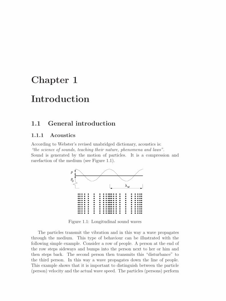
According to Webster’s revised unabridged dictionary, acoustics is:“the science of sounds, teaching their nature, phenomena and laws”.Sound is generated by the motion of particles. It is a compression andrarefaction of the medium (see Figure 1.1).
p
p0
λw
Figure 1.1: Longitudinal sound waves
The particles transmit the vibration and in this way a wave propagatesthrough the medium. This type of behaviour can be illustrated with thefollowing simple example. Consider a row of people. A person at the end ofthe row steps sideways and bumps into the person next to her or him andthen steps back. The second person then transmits this “disturbance” tothe third person. In this way a wave propagates down the line of people.This example shows that it is important to distinguish between the particle(person) velocity and the actual wave speed. The particles (persons) perform

2 Introduction
a small oscillation around their equilibrium position, while the wave propa-gates through the medium 1. In air at atmospheric conditions the speed ofsound is approximately 340 m/s. Standard acoustic waves in air are longi-tudinal waves: the direction of motion of the particles and the propagationdirection of the wave coincide. In other media or situations other types ofwaves may exist.
Due to the compression and rarefaction the motion of the particles isaccompanied by pressure disturbances with amplitude p (see Figure 1.1).The pressure disturbances associated with sound waves are usually smalldisturbances upon a steady state, e.g. atmospheric, condition (in Figure1.1 indicated by p0). Because sound is a mechanical phenomenon, it can-not propagate in vacuum. In the latter case there simply is no medium totransmit the mechanical vibrations.
The most important quantities that characterize a harmonic sound waveare its speed of propagation, its wavelength and its amplitude. The speed ofpropagation depends on the medium of interest and the ambient conditions.The wavelength is the distance after which the pressure pattern is repeated(see figure 1.1). The frequency of the wave is the number of cycles per second.For standard acoustic wave propagation the frequency f and the wavelengthλw are related as:
λw =c0
f(1.1)
where c0 is the undisturbed (adiabatic) speed of sound. The wavelength thusdecreases with increasing frequency. The human ear is able to detect soundin the frequency range between 20 Hz and 20 kHz. For air under atmosphericconditions, this corresponds to wavelengths between roughly 1.7 cm and 17m.
1.1.2 Standard acoustic wave propagation
The mathematical concept to describe the propagation of sound waves, basedon the so-called wave equation, has long been known. It is widely used todescribe for instance sound fields in large enclosures and radiation and scat-tering phenomena. The basis of this acoustic equation is the more general setof fluid dynamics equations: the Navier Stokes equations. This very compli-cated set of non-linear equations can be drastically simplified for the acousticcase. Small perturbations are introduced and mean flow is assumed to bezero. There is no heat exchange between the medium and the surroundingboundary: the process is assumed adiabatic. The medium is homogeneous:
1In the present study the mean flow is zero

1.1 General introduction 3
the properties of the medium are the same throughout the domain. This con-dition is satisfied if the wavelength is large compared to the intermolecularspacing, the so-called mean free path. Finally, the viscosity of the medium,a measure for the “stickyness”, is neglected. Viscosity effects are typicallyimportant in the vicinity of a wall, where the medium sticks to the sur-face. Viscosity is thus usually neglected when describing sound propagationin large enclosures and unconfined spaces. If these assumptions are used,the Navier Stokes equations can be further simplified to a linearized set ofequations. In combination with the equation of continuity and the equationof state, a partial differential equation in terms of the pressure perturba-tion is obtained: the wave equation. This equation forms the basis for thedescription of standard acoustic wave propagation.
1.1.3 Solution techniques for standard acoustic wavepropagation
The wave equation has been extensively studied and consequently a largevariety of solution methods is available. Several analytical techniques weredeveloped. During the last decades the computer has enabled the numericalsimulation of sound fields for complex geometries and boundary conditions(see e.g. [1]). A popular numerical technique, the Finite Element Method(FEM), is based on a volume modelling of the medium. This method is gen-erally accepted and a large amount of knowledge and experience is available.Finite element models have also been developed to describe the propagationof sound in porous media and to describe the behaviour of absorbing walls.The method is usually applied to confined spaces, although for instance “in-finite finite” elements were developed for radiation problems.
Another popular numerical technique is the Boundary Element Method(BEM). This method is based on a surface modelling of the boundaries ofthe medium. In physical terms, the surface of for instance a vibrating panelis covered with a distribution of acoustic monopoles (“acoustic sources”) ordipoles. The strength distribution of these monopoles and dipoles then has tobe calculated. This method is especially suited for unconfined spaces becausethe radiation conditions are automatically satisfied.
Both in FEM and BEM a sufficient number of elements has to be usedper wavelength to accurately describe a signal of interest. Since the wave-length dramatically decreases with increasing frequency, the required numberof elements shows a strong increase. Furthermore the detailed information,provided by the deterministic FEM and BEM approaches, is not very mean-ingful in the high frequency range. For the high frequency range, Statistical

4 Introduction
Energy Analysis was developed. Essentially, this technique is based on aver-aging and energy flows.
Finally, multigrid techniques and multilevel integration techniques areused in acoustical problems. For FEM and BEM, the computational effortsshow a strong increase with problem size. Multilevel algorithms are moreefficient by using the economy of scales. The multigrid techniques are basedon a volume modelling, the equivalent of FEM, while the multilevel integra-tion techniques are based on a boundary integral approach, the equivalent ofBEM.
It can be concluded that a variety of generally accepted models is avail-able to deal with standard acoustic wave propagation. For a more detaileddiscussion the reader is referred to [2].
1.1.4 Viscothermal wave propagation
This is the first important aspect of the present thesis. The key issue is thatthe viscous and thermal effects are now included in the analysis.
Figure 1.2: Sound waves in thin layers or narrow tubes
Consider the propagation of sound in a thin layer or a narrow tube (seeFigure 1.2). At the wall, there is a no-slip condition for the medium: itsticks to the surface. For a thin layer or a narrow tube, this can lead tosignificant boundary layer effects, where viscosity is important. Furthermore,thermal effects can play an important role. For a mathematical description ofviscothermal wave propagation, the Navier Stokes equations and the energyequation are used as a starting point. This time the viscous and thermaleffects are retained in the analysis. The following basic assumptions areused: no mean flow, small perturbations and a homogeneous medium. TheNavier Stokes equations can be simplified using these basic assumptions.
In the literature a seemingly wide variety of models is presented, eachwith their own additional assumptions. An overview of viscothermal modelsfor the propagation of sound in tubes was presented by Tijdeman [3]. Byusing dimensionless parameters, the models were put into perspective. For
1.1 General introduction 5
layer geometries, however, the viscothermal modelling is less well developed,as will be demonstrated in chapter 2.
1.1.5 Solution techniques for viscothermal wave prop-agation
For the propagation of sound in tubes, several analytical and numerical tech-niques are available (see also chapter 2). For layer geometries a number ofanalytical techniques were developed. These methods however are restrictedto very simple geometries and boundary conditions. Recently, a boundaryelement formulation for viscothermal wave propagation in thin layers waspresented by Karra, Ben Tahar, Marquette and Chau [4] and Karra and BenTahar [5]. This model is based on a full linearized Navier Stokes model andis not very efficient for viscothermal wave propagation in layers, as will beshown in chapter 2. To the author’s knowledge no general, efficient solutiontechnique is available for viscothermal wave propagation in thin layers.
1.1.6 Acousto-elasticity
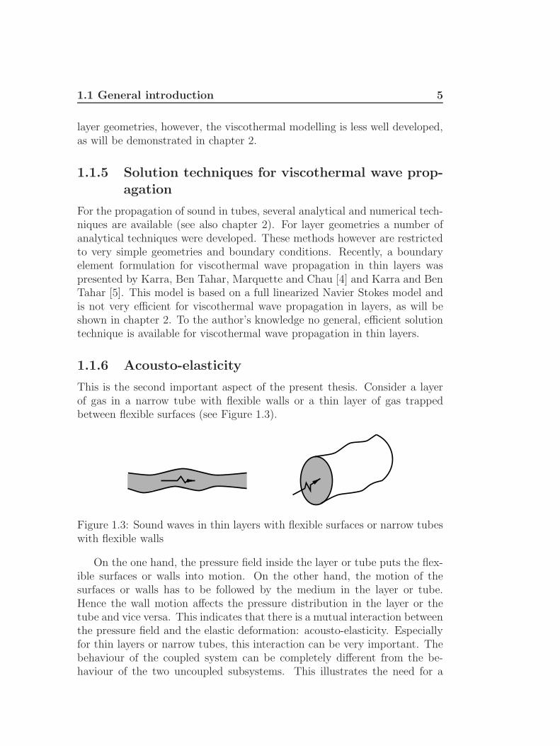
This is the second important aspect of the present thesis. Consider a layerof gas in a narrow tube with flexible walls or a thin layer of gas trappedbetween flexible surfaces (see Figure 1.3).
Figure 1.3: Sound waves in thin layers with flexible surfaces or narrow tubeswith flexible walls
On the one hand, the pressure field inside the layer or tube puts the flex-ible surfaces or walls into motion. On the other hand, the motion of thesurfaces or walls has to be followed by the medium in the layer or tube.Hence the wall motion affects the pressure distribution in the layer or thetube and vice versa. This indicates that there is a mutual interaction betweenthe pressure field and the elastic deformation: acousto-elasticity. Especiallyfor thin layers or narrow tubes, this interaction can be very important. Thebehaviour of the coupled system can be completely different from the be-haviour of the two uncoupled subsystems. This illustrates the need for a

6 Introduction
fully coupled analysis where the motion of the structure and the medium areto be coupled on the interface.
1.1.7 Solution techniques for acousto-elastic problems
The modelling of the dynamical behaviour of flexible structures (in vacuum)is very well developed. Several models are available to deal with a largevariety of problems. The description of the interaction for the standardacoustic case is also well established. Finite element and boundary elementtechniques are widely used to deal with fully coupled acousto-elastic calcula-tions. Reduction techniques, like component mode synthesis, were developedto reduce the computing time.
For the viscothermal case, however, no general, efficient acousto-elasticmodel is available. The boundary element model, presented by Karra andBen Tahar [5] is able to deal with coupled calculations for rotatory symmetricproblems. Their viscothermal model however is not very efficient (see chapter2) and in addition a finite element technique is usually more beneficial forsmall enclosed spaces.
1.1.8 Applications
There is a wide range of applications for the present research. Traditionally,viscothermal models have been used to describe the behaviour of spheri-cal resonators, the propagation of sound waves in tubes, the behaviour ofminiaturized transducers and the squeeze film damping between plates (seechapter 3). In the present study the viscothermal models will also be usedto describe some other applications: the behaviour of a folded stack of solarpanels during launch, the design of an inkjet print head and the acousticbehaviour of double wall panels (see chapter 6).
1.2 Formulation of the problem
Development, implementation, validation and application of a model for thedescription of viscothermal wave propagation, including acousto-elastic in-teraction.
1.3 Outline
As far as the development of new models is concerned, attention will be fo-cused on the viscothermal models, since the structural models are already
1.3 Outline 7
very well developed. In chapter 2 an overview is presented for viscothermalwave propagation. Based on a parameter approach, as presented by Tijdeman[3] for tubes, the various models are put into perspective. The models are allwritten in a general form and therefore apply to different co-ordinate systems(e.g. spherical, cylindrical or cartesian). The low reduced frequency modelof Tijdeman is extended to thin layers for the present study. It is stressedthat the models that are described in chapter 2 are not new. However, forthe present investigation all models were rewritten into the aforementioneddimenionless form. Based on a parameter analysis, the most efficient modelis identified: the low reduced frequency model. Therefore chapter 2 alsoserves as a justification for the emphasis that is placed on the low reducedfrequency model. In order to demonstrate the wide range of applicabilityof the low reduced frequency model, a number of examples from the litera-ture is discussed in chapter 3. In this chapter an overview of fundamentalsolutions and general applications is given. Because the models are writtenin terms of dimensionless parameters and solutions for various co-ordinatesystems are given, this chapter also serves as a solution overview. Chapter4 concerns an experimental validation of the low reduced frequency model.A special large-scale setup with an oscillating solar panel was designed forthis purpose. As a next step, in chapter 5 a new finite element model is de-veloped for fully coupled acousto-elastic calculations including viscothermaleffects. A number of convergence tests were carried out and the model wasexperimentally validated with a special test setup. In chapter 6 the newlydeveloped techniques are used in a number of applications: the behaviour ofstacked solar panels during launch, the design of an inkjet print head and theacoustic behaviour of double wall panels. A preliminary study was carriedout to investigate the influence of obstructions in a thin layer. Finally, theconclusions are presented in chapter 7.

8 Introduction
Chapter 2
Linear viscothermal wavepropagation
2.1 Introduction
The propagation of sound waves with viscothermal effects has been inves-tigated in several scientific disciplines. The propagation of sound waves intubes was investigated already by Kirchhoff and Rayleigh [6]. In tribology,the Reynolds equation is used to calculate the pressure distribution in fluidfilms trapped between moving surfaces. Reynolds’ theory assumes that theinertial effects are negligible: it is based on a so-called creeping flow assump-tion. Increasing machine speeds and the use of gas bearings initiated researchon the role of inertia [7, 8, 9, 10, 11, 12, 13, 14, 15]. In fluid mechanics theprogagation of sound waves in tubes and in particular the steady streamingphenomenon have been extensively discussed [16, 17, 18, 19]. Two early pa-pers on thin film theory in acoustics were presented by Maidanik [20] andUngar and Carbonell [21]. A large number of investigations have been car-ried out since then. Consequently, a seemingly endless variety of models isavailable now to deal with viscothermal effects in acoustic wave propagation.
The variety of models is deceiving. The models that were presented inacoustics can be grouped into three basic categories. Key words in the char-acterization of these models are: pressure gradient across layer thickness ortube cross section, and the incorporation of effects such as compressibilityand thermal conductivity.
The most extensive type of model clearly must be based on a solution ofthe full set of basic equations. This means that, for instance, all the termsin the linearized Navier Stokes equations are taken into account. The secondtype of model incorporates a pressure gradient. However, not all the terms
10 Linear viscothermal wave propagation
in the basic equations are retained. In some models, for instance, thermaleffects are neglected. The simplest model, the low reduced frequency model,assumes a constant pressure across the layer thickness or tube cross section.The effects of inertia, viscosity, compressibility and thermal conductivity areaccounted for. This leads to a very straightforward and useful model.
The main aim of this chapter is to provide a framework for putting modelsfor viscothermal wave propagation into perspective. It is not the intentionof the author to present a list of all papers related to viscothermal wavepropagation. Wave propagation is considered from a standard acousticalpoint of view. Non-linear effects are therefore neglected. For an extensiveoverview of non-linear effects and viscothermal wave propagation the readeris referred to Makarov and Ochmann [22, 23, 24] and Too and Lee [25].Makarov and Ochmann present an overview of the literature, based on morethan 300 references.
The present analysis is based on the use of dimensionless parameters. Itis an extension of the work on the propagation of sound waves in cylindri-cal tubes, as presented by Tijdeman [3]. The three groups of models are allrewritten in a dimensionless form. As a consequence, a number of dimension-less parameters appear in the equations. With the help of these parametersthe range of validity for each group is indicated. Furthermore, for each typeof model a short list of related literature is given. The list offers informationabout parameter ranges and applications. Based on this information, onecan easily determine which model should be used for a given application.Finally, the problem of acousto-elastic coupling, i.e. the mutual interactionbetween vibrating flexible surfaces and thin layers of gas or fluid, is addressedfor each type of model.
2.2 Basic equations 11
2.2 Basic equations
2.2.1 Derivation of equations
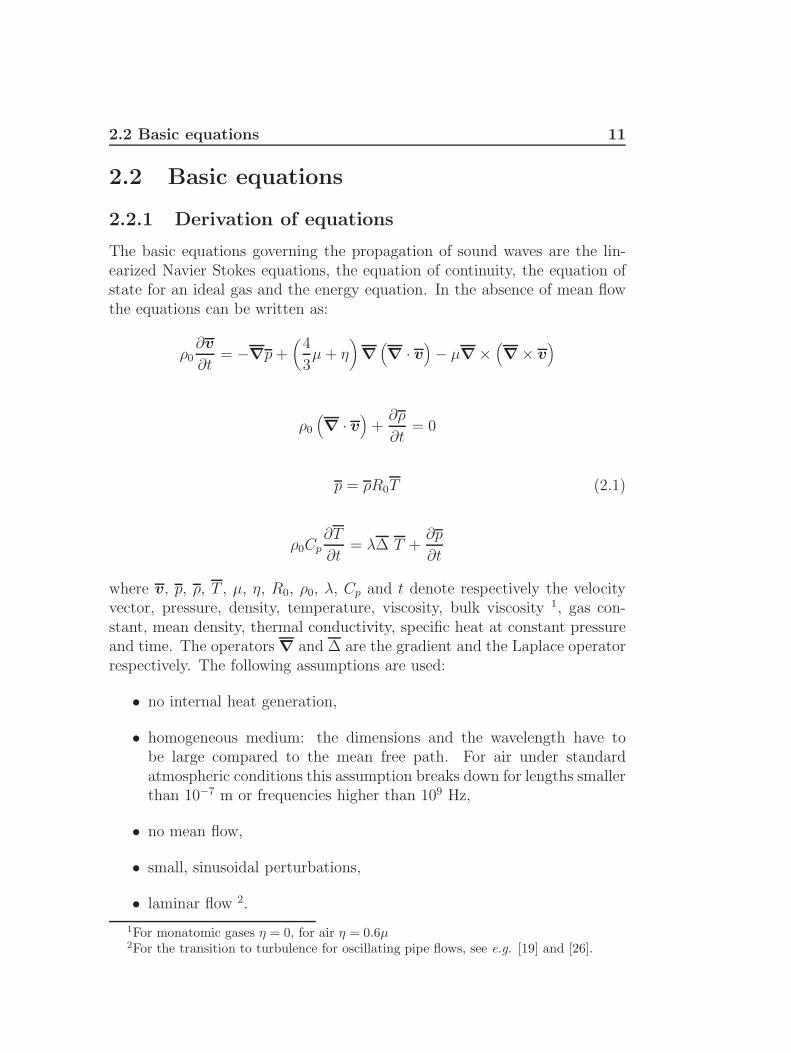
The basic equations governing the propagation of sound waves are the lin-earized Navier Stokes equations, the equation of continuity, the equation ofstate for an ideal gas and the energy equation. In the absence of mean flowthe equations can be written as:
ρ0∂v
∂t= −∇p+
(4
3µ+ η
)∇(∇ · v
)− µ∇×
(∇× v
)
ρ0
(∇ · v
)+∂ρ
∂t= 0
p = ρR0T (2.1)
ρ0Cp∂T
∂t= λ∆ T +
∂p
∂t
where v, p, ρ, T , µ, η, R0, ρ0, λ, Cp and t denote respectively the velocityvector, pressure, density, temperature, viscosity, bulk viscosity 1, gas con-stant, mean density, thermal conductivity, specific heat at constant pressureand time. The operators∇ and ∆ are the gradient and the Laplace operatorrespectively. The following assumptions are used:
• no internal heat generation,
• homogeneous medium: the dimensions and the wavelength have tobe large compared to the mean free path. For air under standardatmospheric conditions this assumption breaks down for lengths smallerthan 10−7 m or frequencies higher than 109 Hz,
• no mean flow,
• small, sinusoidal perturbations,
• laminar flow 2.
1For monatomic gases η = 0, for air η = 0.6µ2For the transition to turbulence for oscillating pipe flows, see e.g. [19] and [26].

12 Linear viscothermal wave propagation
Dimensionless small harmonic perturbations are introduced according to:
v = c0veiωt p = p0
[1 + peiωt
]T = T0 [1 + Teiωt] ρ = ρ0
[1 + ρeiωt
](2.2)
where c0, T0, p0, ω and i are the undisturbed speed of sound, the meantemperature, mean pressure, angular frequency and the imaginary unit. Thegradient and the Laplace operators are non-dimensionalized with a lengthscale l. This length scale can for example represent the layer thickness orthe tube radius. An overview of length scales and operators for variousgeometries is given in Appendix B. At this stage one can write:
∇ = l∇∆ = l2∆ (2.3)
After further linearization the basic equations can be written in the followingdimensionless form 3:
iv = − 1
kγ∇p+
1
s2
(4
3+ ξ
)∇ (∇ · v)− 1
s2∇× (∇× v)
∇ · v + ikρ = 0
p = ρ+ T (2.4)
iT =1
s2σ2∆T + i
[γ − 1
γ
]p
The following dimensionless parameters were introduced 4:
shear wave number s = l
√ρ0ω
µ
reduced frequency k =ωl
c0
3R0 = Cp − Cv4The shear wave number is an unsteady Reynolds number

2.2 Basic equations 13
ratio of specific heats γ =CpCv
(2.5)
square root of the Prandtl number σ =
√µCpλ
viscosity ratio ξ =η
µ
where Cv is the specific heat at constant volume. The dimensionless equationsindicate that the viscothermal wave propagation is governed by a number ofdimensionless parameters. These parameters can be used to characterizedifferent flow regimes. Furthermore, they enable solutions given in the liter-ature to be put into perspective: assumptions or restrictions of models canbe quantified in terms of these parameters.
The parameters γ and σ depend solely on the material properties of thegas. The most important parameters are the shear wave number and thereduced frequency. The shear wave number is a measure for the ratio be-tween the inertial effects and the viscous effects in the gas: it is an unsteadyReynolds number. For large shear wave numbers the inertial effects domi-nate, whereas for low shear wave numbers the viscous effects are dominant.In physical terms the shear wave number represents the ratio between thelength scale, e.g. the layer thickness or tube radius, and the boundary layerthickness. The reduced frequency represents the ratio between the lengthscale and the acoustic wave length. For very low values of the reduced fre-quency, the acoustic wave length is very large compared to the length scalel. The parameters presented in this section are essential for the choice of anappropriate model for a specific situation.
2.2.2 Boundary conditions
In order to solve the set of equations boundary conditions must be imposed.The quantities of interest here are the (dimensionless amplitudes of the)velocity, temperature, pressure and density. Boundary conditions for thedensity are usually not imposed, and will therefore not be considered here.
Velocity
At a gas-wall interface a continuity of velocity is assumed in most cases.Continuity of velocity usually implies that the tangential velocity is zero: ano-slip condition is imposed. The normal velocity is equal to the velocity ofthe wall. In this way the acousto-elastic coupling between vibrating struc-tures and viscothermal gases is established. For rarefied gases investigations

14 Linear viscothermal wave propagation
indicate that it is more appropriate to use a jump in velocity with corre-sponding momentum accommodation coefficients 5 [27, 28]. For gases underatmospheric conditions a simple continuity of velocity condition suffices.
Temperature
The most common boundary conditions are isothermal walls or adiabaticwalls. For an isothermal wall the temperature perturbation is zero, whereasfor an adiabatic wall the gradient of the temperature normal to the wallvanishes. When the product of the specific heat per unit volume and thethermal conductivity of the wall material substantially exceeds the corre-sponding product for the gas, the assumption of isothermal walls is usuallyaccurate (see e.g. [29]).
Again, for rarefied gases it is more appropriate to use a jump condition[27, 28]. This condition allows for a jump in temperature across the gas-wallinterface with a thermal accommodation coefficient. In the literature somemodels were presented to model walls with finite heat conduction properties,see e.g. [30].
A very interesting consequence of thermal effects is the phenomenon ofthermally driven vibrations. As a boundary condition, one could for instanceimpose a varying temperature across the length of a tube. This temperaturegradient drives pressure pulsations in the gas. This effect will not be ad-dressed here: for a detailed discussion the reader is referred to the literature[31, 32, 33, 34, 35, 36, 37, 38].
Pressure
At the ends of a tube or layer boundary conditions can be imposed for thepressure, for instance a pressure release. In the present investigation endeffects are neglected. For a more detailed discussion on this subject thereader is referred to the literature [39, 40, 41, 42, 43, 44].
2.2.3 Geometries and co-ordinate systems
The basic equations were given in terms of gradient and Laplace operators. InAppendix B an overview of length scales, dimensionless co-ordinates, gradientoperators and Laplace operators is given for a number of geometries.
5In this case one assumes a jump condition at the interface, e.g. a velocity slip ortemperature jump. For the temperature the boundary equation then becomes: T − Tw =−L∇T · n, where Tw is the wall temperature, L is related to the thermal accomodationcoefficients and n is the outward normal.

2.3 Full linearized Navier Stokes model 15
2.3 Full linearized Navier Stokes model
2.3.1 Derivation of equations
The most extensive type of model is that obtained by solving the completeset of basic equations. The derivation in this section is based on the paperby Bruneau, Herzog, Kergomard and Polack [45]. Their formulation howeverwas rewritten in terms of dimensionless quantities for the present study. Inorder to solve this problem, the velocity is written as the sum of a rotationalvelocity vv, due to viscous effects, and a solenoidal velocity vl:
v = vv + vl (2.6)
where these satisfy:
∇ · vv = 0 ; ∇× vl = 0 (2.7)
The following relationship was used in this derivation:
∇× (∇× vv) ≡∇ (∇ · vv)− (∇ ·∇)vv = −∆vv (2.8)
Inserting these expressions into the basic equations and taking the rotationand divergence gives the following set of dimensionless equations:
ivl −1
s2
(4
3+ ξ
)∆vl = − 1
kγ∇p
∇ · vl + ikρ = 0
ivv −1
s2∆vv = 0 (2.9)
p = ρ+ T
iT =1
s2σ2∆T + i
[γ − 1
γ
]p
After some algebraic manipulations the following equation can be derived interms of the temperature perturbation:
i
s2σ2
[1 +
iγk2
s2
(4
3+ ξ
)]∆∆T +
[1 +
ik2
s2
[(4
3+ ξ
)+
γ
σ2
]]∆T + k2T = 0
(2.10)

16 Linear viscothermal wave propagation
It can easily be verified that both vl and p also satisfy this equation. Notethat if ξ = 0 in this equation, i.e. the bulk viscosity is neglected, a di-mensionless equation is obtained that was already derived by Kirchhoff andRayleigh [6].
2.3.2 Solution strategy
The equation for the temperature perturbation can be written in a factorizedform: [
∆ + ka2] [
∆ + kh2]T = 0 (2.11)
where ka and kh are the acoustic and entropic wave numbers respectively:
ka2 =
2k2
C1 +√C1
2 − 4C2
; kh2 =
2k2
C1 −√C1
2 − 4C2
(2.12)
where:
C1 =
[1 +
ik2
s2
[(4
3+ ξ
)+
γ
σ2
]]; C2 =
ik2
s2σ2
[1 +
iγk2
s2
(4
3+ ξ
)](2.13)
The solution for the temperature perturbation can be written as:
T = AaTa + AhTh (2.14)
where Ta and Th are referred to as the acoustic and the entropic tempera-ture. The constants Aa and Ah remain to be determined from the boundaryconditions. The quantities Ta and Th are the solutions of:[
∆ + ka2]Ta = 0 ;
[∆ + kh
2]Th = 0 (2.15)
Once the solution for the temperature is known, the values for the velocityvl and the pressure p can be expressed in terms of Aa, Ah, Ta and Th. Oneobtains:
p =
[γ
γ − 1
] [Aa
[1− ika
2
s2
1
σ2
]Ta +Ah
[1− ikh
2
s2
1
σ2
]Th
]
vl = vla + vlh = αaAa∇Ta + αhAh∇Th (2.16)
αa =i
kγ
[γ
γ − 1
] 1− ika
2
s2
1
σ2
1− ika2
s2
(4
3+ ξ
) ; αh =
i
kγ
[γ
γ − 1
] 1− ikh
2
s2
1
σ2
1− ikh2
s2
(4
3+ ξ
)

2.3 Full linearized Navier Stokes model 17
The rotational velocity vv has to be solved from a vector wave equation withwave number kv: [
∆ + kv2]vv = 0 ; kv
2 = −is2 (2.17)
The rotational velocity is related to the effects of viscosity, since the wavenumber is a function of the shear wave number.
In order to solve the full model, solutions must be found to two scalarwave equations for the temperature perturbation and a vector wave equationfor the rotational velocity. With the appropriate boundary conditions thecomplete solution can then be obtained. An analytical solution for this typeof model can only be found for simple geometries and boundary conditions(see sections 2.3.4 and 2.3.5 and chapter 3). For more complex geometriesone has to resort to numerical techniques.
2.3.3 Acoustic and entropic wave numbers
The expressions for ka and kh are rather complex. In the literature theyare often approximated, see e.g. [45]. With the help of the dimensionlessparameters this approximation can be quantified. A Taylor expansion of thedenominator of the wave numbers in terms of k/s gives:
ka2 =
k21 + i
(k
s
)2 [(4
3+ ξ
)+γ − 1
σ2
]−(k
s
)4 (γ − 1
σ2
) [1
σ2−(
4
3+ ξ
)]
kh2 =
−is2σ21−i (γ − 1)
(k
s
)2 [1
σ2−(
4
3+ ξ
)] (2.18)
These expressions are valid for k/s 1: the acoustic wavelength is verylarge compared to the boundary layer thickness. This assumption seems veryreasonable. However, it has important implications that actually eliminatethe need for a full model, as will also be illustrated in section 2.6. If we setk/s = 0 the expressions reduce to:
ka2 = k2 ; kh
2 = −is2σ2 (2.19)
This result shows that the wave number ka is related to acoustic effects.The wave number kh is related to entropy effects, since the product sσ doesnot contain the viscosity µ. However, this separation is only possible fork/s 1. When the acoustic wavelength is of the same order of magnitude as

18 Linear viscothermal wave propagation
the boundary layer thickness, the complete expressions for the wave numberska and kh must be used. In this situation a separation is not possible.
Note that for s 1 the wave numbers kh and kv become very large. Thesolutions for Th and vv approach zero. The value of ka is not affected, sinceit is not a function of the shear wave number. As a consequence, the fulllinearized Navier Stokes model reduces to the standard wave equation.
2.3.4 Acousto-elastic coupling
The motion of the gas can be coupled to the motion of a flexible structure,usually by demanding a continuity of velocity across the interface. In ge-neral this leads to a very complicated set of equations. The full linearizedNavier Stokes model was used in a number of applications, such as sphe-rical resonators or miniaturized transducers, to calculate the acousto-elasticbehaviour of systems.
Spherical resonators are used to determine the acoustical properties ofgases with a high degree of accuracy. Mehl investigated the effect of shellmotion, hereby neglecting viscothermal effects in the gas [46]. Moldover,Mehl and Greenspan [29] used a full linearized Navier Stokes model for thedescription of the acoustic field inside the resonator. A boundary impedancecondition was imposed for the radial velocity in order to account for the effectof shell motion. The models developed by Mehl were used to calculate thisshell impedance.
In some types of miniaturized transducers a vibrating membrane is backedby a rigid electrode, thus entrapping a thin layer of gas. Plantier and Bruneau[47], Bruneau, Bruneau and Hamery [48], Hamery, Bruneau and Bruneau [49]developed analytical models to describe the interaction between (circular)membranes and thin gas layers. Because of the complexity of the problem,their calculations are restricted to geometries with rotatory symmetry. Inorder to overcome this problem, recently Karra, Tahar and Chau [4, 5] pre-sented a boundary element formulation for the propagation of sound wavesin viscothermal gases. Although their paper only concerns an uncoupled testcase, the algorithm is able to deal with fully coupled problems [50]. Theirmethod therefore now offers the possibility to model more complex geome-tries.
In chapter 3 the spherical resonator and the miniaturized transducers arediscussed in more detail.
2.3 Full linearized Navier Stokes model 19
2.3.5 Literature
In Table 2.1 a list of related literature is presented. The list contains infor-mation concerning applications and acousto-elastic coupling. For layer ge-ometries the parameter ranges in the calculations and experiments are given.These values will also be used in section 2.6. For an overview of parametervalues for tubes the reader is referred to Tijdeman [3].

20
Lin
ear
vis
coth
erm
al
wave
pro
pagati
on
Authors Ref Year Application Coupling RemarksMoldover, Mehl, Greenspan [29] 1986 spherical resonator full analytical modelBruneau, Polack, Herzog, [51] 1990 spherical resonator no analytical modelKergomard cylindrical tubesPlantier, Bruneau [47] 1990 circular membrane full analytical model
2.3 · 10−9 ≤ k ≤ 2.3 · 10−3(•)2.9 · 10−6 ≤ k/s ≤ 2.9 · 10−3(•)
Bruneau [52] 1994 membrane no analytical modelHamery, Bruneau, [49] 1994 circular membrane no analytical modelBruneau 4.6 · 10−5 ≤ k ≤ 4.6 · 10−5(•)
9.0 · 10−4 ≤ k/s ≤ 2.8 · 10−2(•)Bruneau, Herzog, [45] 1989 spherical resonator no analytical modelsKergomard, Polack cylindrical tube
plane wallBruneau, Bruneau, [53] 1987 tubes no analytical modelHerzog, KergomardKarra, Tahar [4] 1996 circular membrane no boundary element modelMarquette, Chau 7.9 · 10−3 ≤ k ≤ 1.4 · 10−2(•)
8.5 · 10−3 ≤ k/s ≤ 1.1 · 10−2(•)Karra, Tahar [5] 1997 circular membrane no boundary element model
Case I (h0 = 0.5 mm):1.0 ≤ k ≤ 1.4(•)9.9 · 10−3 ≤ k/s ≤ 1.1 · 10−2(•)Case II (h0 = 1 µm):7.9 · 10−3 ≤ k ≤ 1.4 · 10−2(•)2.7 · 10−2 ≤ k/s ≤ 3.6 · 10−2(•)
Scarton, Rouleau [26] 1973 tubes noTijdeman [3] 1975 tubes noLiang, Scarton [54] 1994 tubes no
Table 2.1: Literature full linearized Navier Stokes models. (•): calculations

2.4 Simplified Navier Stokes models 21
2.4 Simplified Navier Stokes models
In this class of models the effects of compressibility or thermal conductivityare neglected compared with the full model described in section 2.3. Inthis section two models will be discussed in more detail. The two modelswere rewritten in a dimensionless form for this purpose. Other models arealso available, but all simplified Navier Stokes models are inconsistent. Anoverview is presented in section 2.4.4.
2.4.1 Trochidis model
Trochidis [55, 56] introduces the following assumption in addition to the basicassumptions described in section 2.2.1:
• the gas is incompressible: ∇ · v = 0
The dimensionless basic equations (2.4) now reduce to 6:
iv = − 1
kγ∇p− 1
s2∇× (∇× v)
∇ · v = 0 (2.20)
Combining these equations gives:
∆p = 0
[∆− is2
]v =
s2
kγ∇p (2.21)
The equation for the pressure is perhaps strange at first sight. Is does notincorporate any viscothermal terms: it is a regular wave equation for in-compressible gas behaviour. It seems that the pressure can be completelydetermined from this equation. However, the boundary conditions must besatisfied. At a gas-wall interface the velocity must be continuous. Usuallythis means that the tangential velocity is zero and the normal velocity equalsthe velocity of the wall. With equation (2.21) the boundary condition for thevelocity can be expressed in terms of pressure gradients. In this way, viscouseffects are introduced into the model.
Clearly, the full linearized Navier Stokes model reduces to the Trochidismodel for incompressible behaviour. The role of the compressibility depends,among other things, on for example the frequency and the global dimensions.
6The 2D formulation from Trochidis was extended to 3D for the present analysis.

22 Linear viscothermal wave propagation
As an example, consider the squeeze film damping between two plates, as de-scribed by Trochidis. The effects of compressibility become important whenthe acoustic wavelength is of the same order of magnitude as the plate di-mensions. This means that the incompressible model of Trochidis can onlybe used for frequencies for which the acoustic wavelength is very large com-pared to the plate dimensions. In a squeeze film problem, the layer thicknessis very small compared with the plate dimensions. In other words: theacoustic wavelength is also very large compared to the layer thickness. Thepressure will thus not vary much across the layer thickness. The Trochidismodel however incorporates a pressure gradient across the layer thickness.This is a weakness of the model: the assumption of incompressible behaviouron the one hand and the incorporation of a pressure gradient across the layeron the other hand are rather inconsistent for a squeeze film problem.
2.4.2 Moser model
Moser [57] extended the Trochidis model in order to account for the com-pressibility of the gas. However, only the compressibility term in the equationof continuity is considered: the compressibility terms in the linearized NavierStokes equations are neglected. Furthermore, the process is assumed to beadiabatic. Moser in fact introduces the following assumptions in addition tothe basic assumptions described in section 2.2.1:
• incompressible linearized Navier Stokes equations
• adiabatic process
The basic equations (2.4) now reduce to 7:
iv = − 1
kγ∇p− 1
s2∇× (∇× v)
∇ · v + ikρ = 0 (2.22)
p = γρ
Combining these equations gives:
∆p+
k2
1 + i
(k
s
)2
p = 0
7The 2D formulation from Moser was extended to 3D for the present analysis.

2.4 Simplified Navier Stokes models 23
∆ (∇× v)− is2 (∇× v) = 0 (2.23)
In a further analysis, Moser assumes that the acoustic wavelength is verylarge compared to the boundary layer thickness: k/s 1. The wave numberin equation (2.23) then reduces to k2 and thus the equation reduces to thestandard wave equation. In this model the viscous effects are also incorpo-rated through the boundary conditions, if the wave number is approximatedby k2.
This model is not very consistent, since the compressibility terms are notfully accounted for. Furthermore, the thermal effects can play an importantrole. There are indeed several examples where thermal effects do have a sig-nificant influence. For a more sophisticated model that incorporates pressuregradients, the thermal effects should be accounted for as well.
2.4.3 Acousto-elastic coupling
In acoustics the simplified Navier Stokes models were mainly used to cal-culate the squeeze film damping between flexible plates. In the analysis ofTrochidis only one-way coupling is considered: the uncoupled deflections ofthe plates were imposed as boundary conditions for the gas. However, recentexperiments and calculations [58, 59] indicate that thin gas layers can havea significant effect on the coupled vibrational behaviour of a plate-gas layersystem. The eigenfrequencies of the plate are substantially affected by thepresence of the layer, whereas the viscothermal effects induce considerabledamping. The full coupling was accounted for in the analysis of Moser. Ithas to be noted that the models as presented by Trochidis and Moser concern2-dimensional problems.
The interaction between viscous fluids and flexible structures was alsoinvestigated from a more mathematical point of view. Schulkes [60] presenteda finite element method to describe the interaction between a viscous fluidand a flexible structure. He assumed the fluid to be incompressible. For moreliterature related to this topic the reader is referred to Schulkes [60, 61].
2.4.4 Literature
In Table 2.2 a list of papers concerning simplified Navier Stokes models ispresented. Experiments were carried out by several authors. The parameterranges for the layer geometries are also given in the Table.

24
Lin
ear
vis
coth
erm
al
wave
pro
pagati
on
Authors Ref Year Application Coupling RemarksTrochidis [55] 1982 squeeze film one-way incompressible
Case I (air):4.6 · 10−4 ≤ k ≤ 8.8 · 10−2()(•)2.8 · 10−4 ≤ k/s ≤ 2.3 · 10−3()(•)Case II (water):5.3 · 10−4 ≤ k ≤ 4.0 · 10−2()(•)1.7 · 10−5 ≤ k/s ≤ 1.3 · 10−4()(•)
Moser [57] 1980 squeeze film full incompressible Navier Stokes2.3 · 10−5 ≤ k ≤ 2.9 · 10−1(•)9.0 · 10−5 ≤ k/s ≤ 5.1 · 10−3(•)
Schulkes [60] 1990 general full incompressibleChow, Pinnington [62] 1987 squeeze film one-way bulk viscosity terms neglected
(gas) thermal effects neglectedCase I (atmospheric air):2.3 · 10−4 ≤ k ≤ 7.3 · 10−2()(•)2.9 · 10−4 ≤ k/s ≤ 2.9 · 10−3()(•)Case II (air, decompression chamber):3.5 · 10−4 ≤ k ≤ 3.5 · 10−2()(•)2.9 · 10−4 ≤ k/s ≤ 4.9 · 10−3()(•)
Chow, Pinnington [63] 1989 squeeze film one-way bulk viscosity terms neglected(fluid) thermal effects neglected
5.2 · 10−5 ≤ k ≤ 1.3 · 10−1()(•)2.4 · 10−5 ≤ k/s ≤ 2.4 · 10−4()(•)
Table 2.2: Literature simplified Navier Stokes models. (): experiments (•): calculations

2.5 Low reduced frequency model 25
2.5 Low reduced frequency model
2.5.1 Derivation of equations
In the low reduced frequency models some simplifications are introduced thatlead to a relatively simple but very useful model for tubes and layers. In thistheory the propagation directions of the waves and the other directions areseparated. The following assumptions are introduced in addition to the basicassumptions described in section 2.2.1:
• the acoustic wavelength is large compared to the length scale l : k 1
• the acoustic wavelength is large compared to the boundary layer thick-ness: k/s 1
If one introduces these assumptions into the basic equations (2.4), presentedin section 2.2.1, one is left with:
ivpd = − 1
kγ∇pdp+
1
s2∆cdvpd
0 = − 1
kγ∇cdp
∇ · v + ikρ = 0 (2.24)
p = ρ+ T
iT =1
s2σ2∆cdT + i
[γ − 1
γ
]p
where ∇pd, ∆pd and vpd represent the gradient operator, the Laplace op-erator and the velocity vector containing components for the propagationdirections only. The operators ∇cd, ∆cd and vcd contain terms for the otherdirections, i.e. the cross-sectional or thickness directions. Expressions forthese operators for various geometries are given in Appendix B 8. The cross-sectional co-ordinates are denoted by xcd and the propagation co-ordinatesare denoted by xpd.
8Note that a low reduced frequency model does not make sense for a spherical geometry.

26 Linear viscothermal wave propagation
2.5.2 Solution strategy
The second equation of (2.24) indicates that the pressure is a function of thepropagation co-ordinates only: the pressure is constant on a cross sectionor across the layer thickness. Hence, the low reduced frequency models aresometimes referred to as constant pressure models. Using the fact that thepressure does not vary with the cd-co-ordinates, the temperature perturba-tion can be solved from a Poisson type of equation. The general solution foradiabatic or isothermal walls can formally be obtained by Green’s function9.At this stage one can write:
T(sσ,xpd,xcd
)= −
[γ − 1
γ
]p(xpd
)C(sσ,xcd
)(2.25)
For simple geometries, solution of the function C is very straightforward10.For more complex geometries numerical techniques can be used. In the lit-erature several approximation techniques have been developed to describethe propagation of sound waves in tubes with arbitrary cross sections, e.g.[64, 65, 66]. Once the solution for the temperature is obtained, the solutionsfor the velocity and the density can be expressed in a similar way:
vpd(s,xpd,xcd
)= − i
kγA(s,xcd
)∇pdp
(xpd
)
ρ(sσ,xpd,xcd
)= p
(xpd
) [1 +
[γ − 1
γ
]C(sσ,xcd
)]−1
(2.26)
Note that, due to the fact that A and C are functions of the cd-co-ordinates,the velocity, temperature and density are not constant in these directions.The functions A and C determine the shape of the velocity, temperatureand density profiles. For isothermal walls the functions A and C are directlyrelated, whereas for adiabatic walls the function C reduces to a very simpleform. One has:
isothermal walls : C(sσ,xcd
)= A
(sσ,xcd
)adiabatic walls : C
(sσ,xcd
)= −1 (2.27)
9It is also possible to include a finite thermal conductivity of the wall, see e.g. section2.2.2 and [45]. The low reduced frequency model has to be coupled to a model thatdescribes the thermal behaviour of the wall.
10The function C is a function only of the cd-co-ordinates for constant cross-sections.For varying cross sections, the value of C depends also on the pd-co-ordinates.

2.5 Low reduced frequency model 27
The expressions for ρ, T and vpd are now inserted into the equation ofcontinuity. After integration with respect to the cd-co-ordinates and somerearranging one obtains:
∆pdp(xpd
)− k2Γ2p
(xpd
)= −ikn(sσ)Γ2< (2.28)
where:
Γ =
√γ
n (sσ)B (s)
n (sσ) =
[1 +
[γ − 1
γ
]D (sσ)
]−1
B (s) =1
Acd
∫Acd
A(s,xcd
)dAcd (2.29)
D (sσ) =1
Acd
∫Acd
C(sσ,xcd
)dAcd
< =1
Acd
∫∂Acd
v · end∂Acd
where Acd is the cross-sectional area, ∂Acd is the corresponding boundaryand en is the outward normal on ∂Acd. For simple boundary conditions, thefunction D can be obtained from:
isothermal walls : D (sσ) = B (sσ)
adiabatic walls : D (sσ) = −1 (2.30)
The function Γ is the propagation constant. The propagation of sound wavesis affected by thermal effects, accounted for in the function n (sσ), and viscouseffects, accounted for in the functionB (s). On the right hand side of equation(2.28) a source term is present due to the squeeze motion of the walls. InTables B.1, B.2, B.3 and B.4 in Appendix B the expressions are listed forvarious geometries and isothermal wall conditions for the functions A andB. The Tables also contain the asymptotic values of the functions for lowand high values of the corresponding argument. It can easily be shown thatfor low values of the shear wave number 11 the low reduced frequency modelreduces to a linearized form of the Reynolds equation. For high shear wavenumbers the low reduced frequency model reduces to a modified form of thewave equation. The modification is due to the fact that the low reducedfrequency model is associated with a constant pressure in the cd-directions.
11Considering σ as a constant.
28 Linear viscothermal wave propagation
2.5.3 Physical interpretation
Velocity profile
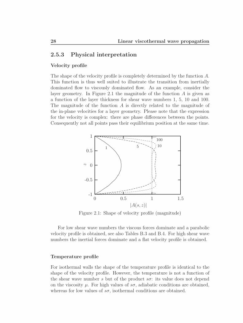
The shape of the velocity profile is completely determined by the function A.This function is thus well suited to illustrate the transition from inertiallydominated flow to viscously dominated flow. As an example, consider thelayer geometry. In Figure 2.1 the magnitude of the function A is given asa function of the layer thickness for shear wave numbers 1, 5, 10 and 100.The magnitude of the function A is directly related to the magnitude ofthe in-plane velocities for a layer geometry. Please note that the expressionfor the velocity is complex: there are phase differences between the points.Consequently not all points pass their equilibrium position at the same time.
1001051
|A(s, z)|
z
1.510.50
1
0.5
0
-0.5
-1
Figure 2.1: Shape of velocity profile (magnitude)
For low shear wave numbers the viscous forces dominate and a parabolicvelocity profile is obtained, see also Tables B.3 and B.4. For high shear wavenumbers the inertial forces dominate and a flat velocity profile is obtained.
Temperature profile
For isothermal walls the shape of the temperature profile is identical to theshape of the velocity profile. However, the temperature is not a function ofthe shear wave number s but of the product sσ: its value does not dependon the viscosity µ. For high values of sσ, adiabatic conditions are obtained,whereas for low values of sσ, isothermal conditions are obtained.

2.5 Low reduced frequency model 29
Polytropic constant
According to equation (2.26) the density and the pressure are related. If thisexpression is integrated with respect to the cd-co-ordinates one obtains:
ρ = p
[1 +
[γ − 1
γ
]D (sσ)
]−1
(2.31)
The same result would have been obtained if, instead of using the energyequation and the equation of state, a polytropic law had been used:
p
ρ n(sσ)= constant (2.32)
where n(sσ) is the polytropic constant that relates density and pressure, seeequation (2.29). Note however that this only holds in integrated sense: rela-tion (2.31) was obtained by integration with respect to the cd-co-ordinates.As an example, the magnitude and the phase angle for the layer geometryare given as a function of sσ in Figure 2.2. For low values n(sσ) reduces to1, i.e. isothermal conditions. For high values of sσ it takes the value of γcorresponding to adiabatic conditions.
sσ
|n(sσ
)|
1001010.1
1.4
1.3
1.2
1.1
1
sσ
arg
(n(sσ
))(
)
1001010.1
10
5
0
Figure 2.2: Magnitude and phase angle of polytropic constant for air(γ = 1.4)
2.5.4 Acousto-elastic coupling
The low reduced frequency model results in a relatively simple equation forthe pressure. Because of the simplicity of the gas model, it is relatively easyto incorporate the full acousto-elastic coupling. Several investigations are

30 Linear viscothermal wave propagation
available which deal with fully coupled calculations, most of them for thesqueeze film problem.
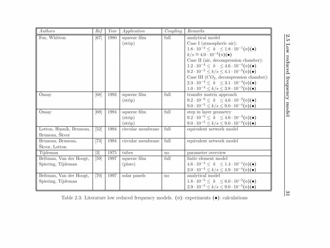
Fox and Whitton [67] and Onsay [68, 69] presented models to describe theinteraction between a vibrating strip and a gas layer. The model of Onsaywas based on a transfer matrix approach: an efficient model for the stripproblem. Fox and Whitton, and Onsay, carried out experiments, showingsubstantial frequency shifts and significant damping.
Recently, Beltman, Van der Hoogt, Spiering and Tijdeman [70, 59, 71,58, 72] presented a finite element model for fully coupled calculations forthe squeeze film problem. A new viscothermal acoustic finite element wasdeveloped, based on the low reduced frequency model. This element canbe coupled to structural elements, enabling fully coupled calculations forcomplex geometries. Furthermore, the layer thickness can be chosen for eachelement. This enables calculations for problems with varying layer thickness.The finite element model was validated with experiments on an airtight boxwith a flexible coverplate. In this case there was a strong interaction betweenthe vibrating, flexible plate and the closed air layer. Eigenfrequency anddamping of the plate were measured as a function of the thickness of the airlayer. Substantial frequency shifts and large damping values were observed.In chapter 5 a more detailed discussion is given of these results.
2.5.5 Literature
In Table 2.3 the recent literature on the low reduced frequency models issummarized. For layer geometries the ranges of dimensionless parametersare also given.
2.5
Low
reduce
dfre
quency
model
31
Authors Ref Year Application Coupling RemarksFox, Whitton [67] 1980 squeeze film full analytical model
(strip) Case I (atmospheric air):1.8 · 10−3 ≤ k ≤ 1.8 · 10−1()(•)k/s ∼= 4.0 · 10−4()(•)Case II (air, decompression chamber):1.2 · 10−4 ≤ k ≤ 4.6 · 10−4()(•)9.2 · 10−5 ≤ k/s ≤ 4.1 · 10−3()(•)Case III (CO2, decompression chamber):2.3 · 10−4 ≤ k ≤ 3.1 · 10−4()(•)1.0 · 10−4 ≤ k/s ≤ 3.8 · 10−3()(•)
Onsay [68] 1993 squeeze film full transfer matrix approach(strip) 9.2 · 10−6 ≤ k ≤ 4.6 · 10−3()(•)
9.0 · 10−5 ≤ k/s ≤ 9.0 · 10−4()(•)Onsay [69] 1994 squeeze film full step in layer geometry
(strip) 9.2 · 10−5 ≤ k ≤ 4.6 · 10−3()(•)(strip) 9.0 · 10−5 ≤ k/s ≤ 9.0 · 10−4()(•)
Lotton, Husnık, Bruneau, [52] 1994 circular membrane full equivalent network modelBruneau, SkvorBruneau, Bruneau, [73] 1994 circular membrane full equivalent network modelSkvor, LottonTijdeman [3] 1975 tubes no parameter overviewBeltman, Van der Hoogt, [59] 1997 squeeze film full finite element modelSpiering, Tijdeman (plate) 4.6 · 10−4 ≤ k ≤ 1.4 · 10−1()(•)
2.0 · 10−4 ≤ k/s ≤ 4.9 · 10−4()(•)Beltman, Van der Hoogt, [70] 1997 solar panels no analytical modelSpiering, Tijdeman 1.8 · 10−5 ≤ k ≤ 6.0 · 10−2()(•)
2.9 · 10−5 ≤ k/s ≤ 9.0 · 10−5()(•)
Table 2.3: Literature low reduced frequency models. (): experiments (•): calculations

32 Linear viscothermal wave propagation
2.6 Dimensionless parameters
2.6.1 Validity of models
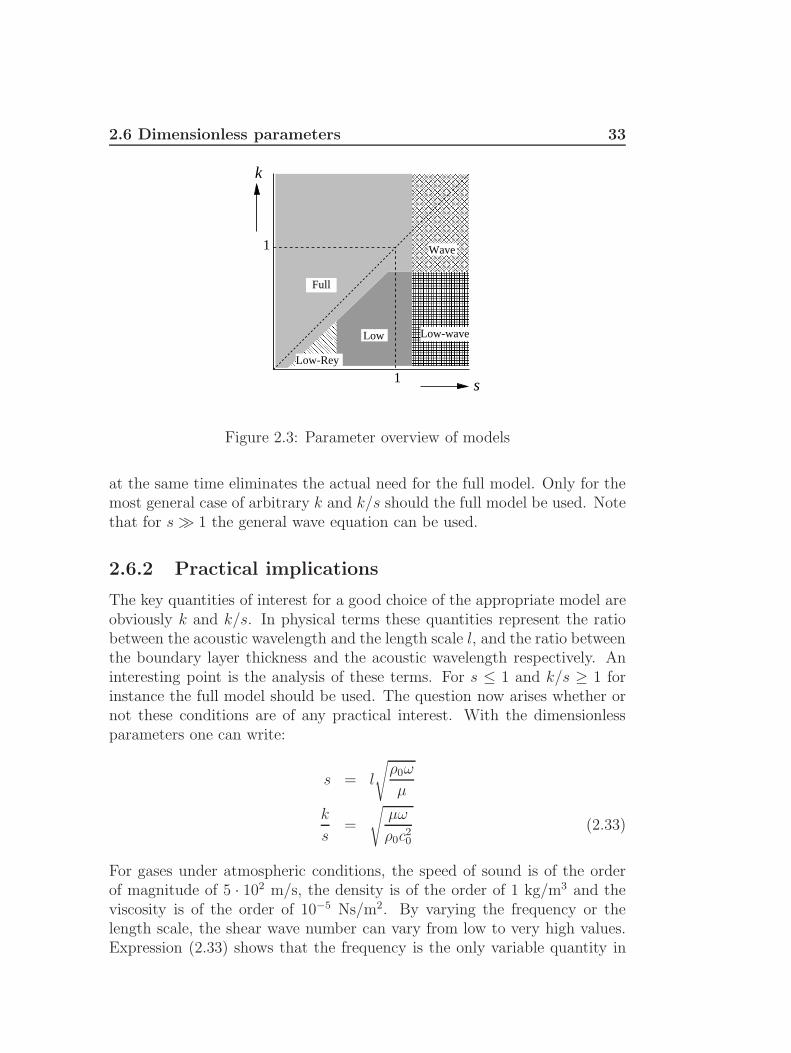
In the sections 2.3, 2.4 and 2.5 three types of models were discussed forthe modelling of viscothermal wave propagation. The most simple type ofmodel, the low reduced frequency model, is show to be valid for k 1and k/s 1. As pointed out in section 2.4, the validity of the simplifiedNavier Stokes models is difficult to quantify. These models incorporate someadditional effects compared to the low reduced frequency models. However,a parameter analysis shows that if a more sophisticated model is desired, infact all the terms have to be accounted for. The complete parameter rangeis covered by the low reduced frequency model and the full linearized NavierStokes model. Summarizing the ranges of validity for the linear viscothermalmodels and the general wave equation:
• s 1wave equation (Wave)
• k 1 and k/s 1low reduced frequency (Low)
• k 1 and k/s 1 and s 1low reduced frequency, Reynolds equation (Low-Rey)
• k 1 and k/s 1 and s 1low reduced frequency, modified wave equation (Low-wave)
• arbitrary k and sfull linearized Navier Stokes (Full) 12
A graphical representation of these ranges of validity is given in Figure 2.3.It is stressed that in each area the most efficient model is given. One couldfor instance use the full model for all situations, but clearly for k 1 andk/s 1 the low reduced frequency model is far more efficient.
For the case of arbitrary k but k/s 1 the simplified wave numbers,as described in section 2.3.3 could be used. However, assuming k/s 1immediately suggests that another model, i.e. the low reduced, modifiedwave or wave, would be more efficient (see Figure 2.3). This assumption,which is often used by authors who use a full linearized Navier Stokes model,
12The full linearized Navier Stokes with simplified wave numbers is valid for k/s 1.It can easily be seen in the graph that this is not an efficient model. Hence, it is notincluded.
2.6 Dimensionless parameters 33
Low-Rey
Low Low-wave
s
1
1
k
Full
Wave
Figure 2.3: Parameter overview of models
at the same time eliminates the actual need for the full model. Only for themost general case of arbitrary k and k/s should the full model be used. Notethat for s 1 the general wave equation can be used.
2.6.2 Practical implications
The key quantities of interest for a good choice of the appropriate model areobviously k and k/s. In physical terms these quantities represent the ratiobetween the acoustic wavelength and the length scale l, and the ratio betweenthe boundary layer thickness and the acoustic wavelength respectively. Aninteresting point is the analysis of these terms. For s ≤ 1 and k/s ≥ 1 forinstance the full model should be used. The question now arises whether ornot these conditions are of any practical interest. With the dimensionlessparameters one can write:
s = l
√ρ0ω
µ
k
s=
√µω
ρ0c20
(2.33)
For gases under atmospheric conditions, the speed of sound is of the orderof magnitude of 5 · 102 m/s, the density is of the order of 1 kg/m3 and theviscosity is of the order of 10−5 Ns/m2. By varying the frequency or thelength scale, the shear wave number can vary from low to very high values.Expression (2.33) shows that the frequency is the only variable quantity in

34 Linear viscothermal wave propagation
k/s: it does not depend on the length scale l. For gases under atmosphericconditions, k/s exceeds unity only for frequencies higher than 109 Hz. How-ever, for these high frequencies the medium can no longer be regarded ashomogeneous and one of the basic assumptions described in section 2.2.1, isviolated.
This can be illustrated with the following simple example. Using expres-sion (2.33), the basic conditions l > 10−7 m and f < 109 Hz can be expressedin terms of k/s and s:
f < 109 Hz :
(k
s
)<
√2πµ
ρ0c20
· 109
l > 10−7 m : s >ρ0c0
µ· 10−7
(k
s
)(2.34)
For air under atmospheric conditions this gives:(k
s
)< 0.3π ; s > 2.24
(k
s
)(2.35)
Thus, the full linearized Navier Stokes model is not even valid in the majorrange where it should be of use for air under atmospheric conditions.
For fluids this reasoning also holds. The quantity k/s contains the ratiobetween the viscosity and the density. For fluids the viscosity is higher, butcompared to gases the ratio between viscosity and density is of the sameorder of magnitude. Furthermore, the speed of sound in fluids is generallyhigher. This implies that for fluids the condition k/s 1 will also usuallybe satisfied. If this condition is not satisfied one has to ensure that the basicassumptions are not violated.
This simple analysis shows that the practical importance of the full modelis very limited. Only under extreme conditions, e.g. at low temperatures orlow pressures, one encounters situations were the full model should be used13.However, one has to ensure that the basic assumptions are not violated inthese cases. This leads to the perhaps surprising conclusion that for gasesunder atmospheric conditions the full linearized Navier Stokes model is notvalid in the parameter range where it should be of use. Most viscothermalproblems can be handled with the low reduced frequency models. In fact, anumber of papers indicate the necessity of a full model because of the highfrequencies involved, whereas a low reduced frequency model would havebeen sufficient [47, 49, 4]. Some examples will be presented in chapter 3.
13For these cases situations are encountered where the jump conditions must be appliedat the boundaries, see section 2.2.2

2.6 Dimensionless parameters 35
2.6.3 Overview of the literature for layers
The dimensionless parameters are used to analyse the literature for the layergeometry. The overview is based on the references presented in Tables 2.1,2.2 and 2.3. For this purpose, the values of the dimensionless parametersat which the calculations and experiments were performed were determinedfrom the data given in the references [47, 49, 4, 55, 57, 62, 63, 67, 68, 69, 59,71]
s
k
104103102101110−110−210−310−4
101
1
10−1
10−2
10−3
10−4
10−5
Figure 2.4: Dimensionless parameters in the literature. Calculations ( ),experiments (−−)
The graph clearly shows that for all investigations the low reduced fre-quency models, modified wave equation models or general wave equationmodels would have been sufficient. None of the present cases required amore sophisticated model, such as the full linearized Navier Stokes model.The conclusion to be drawn from this Figure is that, although a variety ofmodels has been developed, this was not necessary when taking a critical lookat the dimensionless parameters. Some investigations mentioned in Tables2.1 and 2.2 could have been carried out with much simpler models. Analysisof the values of the parameters, listed in the Tables, also immediately revealsthat the conditions for the use of simpler models are satisfied.

36 Linear viscothermal wave propagation
2.7 Conclusions
The conclusions to be drawn from the present investigation are as follows:
• viscothermal wave propagation is governed by a number of dimension-less parameters. The most important parameters are the shear wavenumber, s, and the reduced frequency, k;
• the viscothermal models presented in the literature, can be groupedinto three categories: full linearized Navier Stokes models, simplifiedNavier Stokes models and low reduced frequency models. The range ofvalidity of the models is governed by the values of k and k/s;
• the full linearized Navier Stokes model should only be used under ex-treme conditions. For gases under atmospheric conditions, this modelis not even valid in the range of use because the basic assumptions areviolated;
• the assumption of small k/s, as often used in the literature concerningfull models, actually eliminates the need for a full model;
• the simplified Navier Stokes models are redundant: the complete pa-rameter range is covered by the other models;
• the low reduced frequency model can be used for most problems. Be-cause of the simplicity of this model, models are already available thatinclude the full acousto-elastic coupling for complex geometries. Themodel is valid for k 1 and k/s 1;
• in the literature a variety of models was presented for the squeeze filmdamping problem. Several authors stated that for miniaturized trans-ducers, the full model had to be used because of the high frequenciesinvolved. An analysis of the parameters learns that for all literatureconcerning squeeze film problems, treated in this chapter, a simple lowreduced frequency model is sufficient and the most efficient.

Chapter 3
Fundamental solutions
3.1 Introduction
In chapter 2 an overview of theories for viscothermal wave propagation waspresented. As a next step, the theory is applied to present solutions for thebehaviour of spherical resonators, the propagation of sound in tubes, thebehaviour of miniaturized transducers and squeeze film damping betweenflexible plates or membranes. Analytical solutions for the full model wereobtained for a spherical geometry, a circular tube geometry and a layer ge-ometry. The results of these models are compared with results from simplermodels, like the low reduced frequency model. All solutions are written interms of dimensionless parameters. The use of these parameters leads tosome interesting observations.
The author would like to stress that it is not his intention to give anextensive and very detailed description of all the aspects for each applica-tion. The present range of applications covers the general application field oflinear viscothermal models. Furthermore, solutions are presented for a rangeof geometries. Thus, the main aim of this chapter is to present an applica-tion overview and a solution overview of linear viscothermal models. Thetheory and the solutions are quite general and can easily be applied to othersituations, because the expressions are all written in terms of dimensionlessparameters.

38 Fundamental solutions
3.2 Spherical resonator
3.2.1 Introduction
Spherical resonators are used to determine the properties of gases, such asthe speed of sound, with a high degree of accuracy, see e.g. Moldover, Mehland Greenspan [29]. In Figure 3.1 a schematic drawing is presented of aspherical resonator.
Vent
Source
Transducer
R
Argon
Figure 3.1: Schematic drawing of a spherical resonator
The sphere consists of two parts that are bolted together. The acousticeigenfrequencies of the enclosed volume are used to determine the propertiesof the gas under different conditions. Because of the spherical geometry, ananalytical solution can be obtained for the full linearized Navier Stokes modelas will be described in sections 3.2.2 to 3.2.5. However, the resonator containsa number of small disturbances: vent holes, transducers, transducer holes anda source. Although both parts of the shell are firmly bolted together, a smallseam can remain between the two parts. In order to account for the presenceof these disturbances, some suggestions to extend the model are introducedin section 3.2.6. Finally, an example with Argon as a gas will be presentedin section 3.2.7.
The derivation of the equations is based on the work by Moldover, Mehland Greenspan [29]. The spherical resonator was also described by Bruneau,Polack, Herzog and Kergomard [51], Bruneau, Herzog, Kergomard and Po-lack [45] and Mehl [46, 74, 75]. The models were rewritten in terms ofdimensionless quantities for the present study.

3.2 Spherical resonator 39
3.2.2 Basic equations
In order to solve the full linearized Navier Stokes model, two scalar waveequations and one vector wave equation have to be solved (see chapter 2). Ina spherical co-ordinate system (r, θ, φ):
[∆ + ka
2]Ta = 0 ;
[∆ + kh
2]Th = 0 ;
[∆ + kv
2]vv = 0 (3.1)
3.2.3 Solution of the scalar wave equations
The solution of the scalar wave equations can be obtained by a straightfor-ward separation of variables:
Ta = jn (kar)Ymn (θ, φ) ; Th = jn (khr)Ymn (θ, φ) (3.2)
where Ymn (θ, φ) is a spherical harmonic function and jn (kar) is a sphericalBessel function. The spherical Bessel function is related to the fractionalBessel function according to [76]:
jn (kar) =1√rJn+ 1
2(kar) (3.3)
The solution for the temperature is:
T = Aajn (kar)Ymn (θ, φ) +Ahjn (khr)Ymn (θ, φ) (3.4)
The solenoidal velocity can be obtained from:
vl = vla + vlh = αaAa∇Ta + αhAh∇Th (3.5)
This gives:
vl =
[αaAa
∂jn (kar)
∂r+ αhAh
∂jn (khr)
∂r
]Ymn (θ, φ)er
+ [αaAajn (kar) + αhAhjn (khr)]1
r
∂Ymn (θ, φ)
∂θeθ (3.6)
+ [αaAajn (kar) + αhAhjn (khr)]1
rsin(θ)
∂Ymn (θ, φ)
∂φeφ
The pressure is:
p =
[γ
γ − 1
] [Aa
[1− ika
2
s2σ2
]jn (kar) +Ah
[1− ikh
2
s2σ2
]jn (khr)
]Ymn (θ, φ)
(3.7)

40 Fundamental solutions
3.2.4 Solution of the vector wave equation
The solution for the vector wave equation can be obtained from the solutionof the scalar wave equation. For the present case the solution is, see Morseand Feshbach [77]:
vv = W1∇× [errjn (kvr)Ymn (θ, φ)]
+ W2∇×∇× [errjn (kvr)Ymn (θ, φ)] (3.8)
where W1 and W2 are constants that remain to be determined from theboundary conditions. After some algebra one obtains:
vv = W1 [−rjn (kvr)]1
rsin(θ)
∂Ymn (θ, φ)
∂φeθ
+ W1 [rjn (kvr)]1
r
∂Ymn (θ, φ)
∂θeφ
+ W2
[n(n+ 1)
rjn (kvr)
]Ymn (θ, φ)er (3.9)
+ W2
[∂
∂r(rjn (kvr))
]1
r
∂Ymn (θ, φ)
∂θeθ
+ W2
[∂
∂r(rjn (kvr))
]1
rsin(θ)
∂Ymn (θ, φ)
∂φeφ
3.2.5 Rigid sphere with isothermal walls
The boundary conditions for the present case for r = 1 are:
T = 0 ; v = vl + vv = 0 (3.10)
The following equation for the spherical resonator is obtained:
[1− αh
αa
] n(n+ 1)
1 +1
jn (kv)
∂jn (kvr)
∂r
∣∣∣∣∣r=1
= (3.11)
1
jn (ka)
∂jn (kar)
∂r
∣∣∣∣∣r=1
−(αhαa
)1
jn (kh)
∂jn (khr)
∂r
∣∣∣∣∣r=1
The eigenfrequencies of the gas in the resonator can be calculated from thisequation. In experiments, a frequency response function is measured. Thefrequency response of the resonator is calculated by expressing the internalacoustic field in terms of the acoustic eigenmodes. The participation factorscan then be calculated, see e.g. [29].
3.2 Spherical resonator 41
3.2.6 Model extensions
Shell motion
As a boundary condition, a zero velocity was imposed for the gas at theshell wall. The shell however can deform under the applied pressure. Mehl[46] developed a model which describes the shell behaviour in terms of animpedance. The effect of shell motion can thus be incorporated in the modelby imposing the shell impedance as a boundary condition for the radial ve-locity and the pressure at the shell wall.
Holes in the shell
The holes will affect the acoustic field inside the resonator. One can dis-tinguish several types of holes, depending on the type of termination. Forvent holes, the circular tube is terminated by a radiation or pressure releasecondition. For the transducer holes, the tube is terminated by the effectiveimpedance of the transducer itself. The propagation of sound waves in acircular tube is governed by the dimensionless parameters. With these pa-rameters, the most efficient model can be identified. The acoustic impedanceof the tube with its termination can be calculated and thus the impedance atthe entrance of the tube is known. As a consequence, there is a non-uniformboundary impedance condition for the gas in the resonator.
Seam
A small gap at the junction between the two hemispheres can affect the acous-tical properties of the resonator. In this case one deals with the propagationof sound waves between parallel surfaces. Again, based on the dimensionlessparameters for this layer geometry one can easily identify the model thatshould be used. The effective impedance of the gap between the hemispherescan then be calculated.
3.2.7 Example: eigenfrequencies of spherical resonator
The properties of the Argon gas and the spherical resonator are (accordingto the case described by Moldover, Mehl and Greenspan [29]):
c0 = 319 m/s ; ρ0 = 1.60 kg/m3
Cp = 528 J/kgK ; γ =5
3(3.12)
λ = 16.7 · 10−3 W/mK ; µ = 22.7 · 10−6 Ns/m2
ξ = 0 ; R = 0.0635 m
42 Fundamental solutions
The bulk viscosity is zero and the ratio of specific heats is equal to 53
fora monatomic (ideal) gas like argon. The eigenfrequencies of the resonatorwere calculated with a simple numerical procedure (see Appendix C). Theeigenfrequencies can be divided into groups. For each value of n there areseveral solutions to the equation. The solutions are denoted here as “ns”,where n is the order of the spherical Bessel function and s is the s-th root.The roots are arranged in ascending order. The results for the n = 0, n = 1and n = 2 modes are given in Table 3.1.
“ns” Eigenfrequency (Hz)wave equation full model
01 0 002 3593 3592 + 0.802i03 6177 6175 + 1.073i04 8718 8717 + 1.305i11 1664 1663 + 1.587i12 4750 4748 + 1.054i13 7360 7359 + 1.246i14 9918 9916 + 1.449i21 2630 2628 + 1.988i22 5817 5816 + 1.363i23 8482 8481 + 1.460i24 11069 11067 + 1.623i
Table 3.1: Eigenfrequencies spherical resonator
The Table shows that the eigenfrequencies for the full model are complex.The imaginary part however is very small compared to the real part. Thereal part of the frequency is almost equal to the frequency that is obtainedwith the wave equation. The viscous and thermal effects only seem to havea small effect on the acoustical eigenfrequencies of the resonator. However,the shifts in frequency have to be related to the accuracy of the experiment.In fact, according to the literature a frequency shift of several Hz can bedenoted as “significant”. The resonance half width, which is equal to theimaginary part of the eigenfrequency, is measured in the experiments. Theviscous and thermal effects partly determine the imaginary component of thefrequency. For a good model, however, the motion of the shell wall must beincluded for example by using the impedance approach.
3.3 Circular tubes 43
3.3 Circular tubes
3.3.1 Introduction
The propagation of sound waves in tubes was already investigated by Kirch-hoff and Rayleigh, see e.g. [6]. A large amount of literature is availableon this subject, dealing with full linearized Navier Stokes models, simpli-fied models and low reduced frequency models. For an overview of modelsin terms of dimensionless parameters the reader is referred to Tijdeman [3],whose paper was also one of the first in which numerical results for the fun-damental mode (m=0) were presented which took into account the influenceof thermal effects. The theory, presented in chapter 2, will now be appliedto describe the propagation of sound waves in circular tubes. A solutionfor the full linearized Navier Stokes model is given. Extending the work ofTijdeman, the present solution includes circumferential harmonic waves ofinteger order m and the effects of bulk viscosity. The results for the case ofm = 0 and zero bulk viscosity are compared with the results presented byTijdeman.
3.3.2 Full linearized Navier Stokes model
Basic equations
In order to solve the full linearized Navier Stokes model, two scalar waveequations and one vector wave equation have to be solved (see chapter 2). Ina cylindrical co-ordinate system (r, θ, x):[
∆ + ka2]Ta = 0 ;
[∆ + kh
2]Th = 0 ;
[∆ + kv
2]vv = 0 (3.13)
Solution of the scalar wave equation
The solution of the scalar wave equations can be obtained by a straightfor-ward separation of variables:
Ta = Jm (karr) fm (θ, x) ; Th = Jm (khrr) fm (θ, x) (3.14)
where:fm (θ, x) =
[C1e
−imθ + C2eimθ] [C3e
−Γx + C4eΓx]
kar =√ka
2 + k2Γ2 ; khr =√kh
2 + k2Γ2 (3.15)
The function fm (θ, x) consists of circumferential harmonics of integer orderm that are travelling in the +x and the −x-directions. The quantity Γ is the
44 Fundamental solutions
propagation constant. The solution for the temperature is:
T = AaJm (karr) fm (θ, x) + AhJm (khrr) fm (θ, x) (3.16)
The solenoidal velocity can be obtained from:
vl = vla + vlh = αaAa∇Ta +Ahαh∇Th (3.17)
This gives:
vl =
[αaAa
∂Jm (karr)
∂r+ αhAh
∂Jm (khrr)
∂r
]fm (θ, x) er
+ [αaAaJm (karr) + αhAhJm (khrr)]1
r
∂fm (θ, x)
∂θeθ
+ [αaAaJm (karr) + αhAhJm (khrr)] k∂fm (θ, x)
∂xex
(3.18)
The pressure is:
p =
[γ
γ − 1
] [Aa
[1− ika
2
s2σ2
]Jm (karr) +Ah
[1− ikh
2
s2σ2
]Jm (khrr)
]fm (θ, x)
(3.19)
Solution of the vector wave equation
The solution of the vector wave equation is, see Morse and Feshbach [77]:
vv = W1∇× [exJm (kvrr) fm (θ, x)]
+ W2∇×∇× [exJm (kvrr) fm (θ, x)] (3.20)
where W1 and W2 are constants that remain to be determined from theboundary conditions, and:
kvr =√kv
2 + k2Γ2 (3.21)
After some algebra one obtains:
vv = W1 [Jm (kvrr)]1
r
∂fm (θ, x)
∂θer −W1
[Jm (kvrr)
∂r
]fm (θ, x) eθ
+ W2
[(kv
2 + k2Γ2)Jm (kvrr)
]fm (θ, x) ex
+ W2 [Jm (kvrr)] k1
r
∂2fm (θ, x)
∂θ∂xeθ
+ W2
[∂Jm (kvrr)
∂r
]k∂fm (θ, x)
∂xex (3.22)

3.3 Circular tubes 45
Dispersion equation
For a rigid tube with isothermal walls, the following boundary conditionsapply for r = 1:
T = 0 ; v = vv + vl = 0 (3.23)
After some algebraic manipulations one obtains the following dispersion equa-tion:
[1− αh
αa
]kv
2
kv2 + k2Γ2
m2
1
Jm (kvr)
∂Jm (kvrr)
∂r
∣∣∣∣∣1
+k2Γ2
kv2
1
Jm (kvr)
∂Jm (kvrr)
∂r
∣∣∣∣∣1
1
Jm (kar)
∂Jm (karr)
∂r
∣∣∣∣∣1
− αhαa
∂Jm (khrr)
∂r
∣∣∣∣∣1
Jm (khr)(3.24)
For given values of the dimensionless parameters and the order m, the valueof the (complex) propagation constant Γ can be solved from this equation.
3.3.3 Low reduced frequency model
For a circular tube with isothermal walls, the low reduced frequency solutionfor the pressure (see chapter 2 and Appendix B) is:
p = C1e−Γx + C2e
Γx (3.25)
Γ =
√γ
n (sσ)B (s)(3.26)
where:
n (sσ) =
[1 +
[γ − 1
γ
]B (sσ)
]−1
B (s) =J2
(si√i)
J0
(si√i) (3.27)
The propagation of waves is governed by the value of the propagation con-stant Γ. There are two waves: one travelling in the negative x-direction andone travelling in the positive x-direction. Note that the pressure is constantacross the cross section of the tube in the low reduced frequency model.

46 Fundamental solutions
3.3.4 Example: propagation constant
m = 0
Consider the case m = 0, i.e. there is no pressure variation in the circumfer-ential direction. The full linearized Navier Stokes model was used to calculatethe value of the propagation constant for different values of k and s. Whenk 1 and k/s 1 the solution of the full model should converge to thelow reduced frequency solution for Γ. Note that the propagation constantdoes not depend on the value of the reduced frequency k in the low reducedfrequency model.
The calculated values for ξ = 0 and ξ = 0.6 for air under atmosphericconditions (γ = 1.4 and σ =
√0.71) are given in Figures 3.2, 3.3, 3.4 and 3.5.
The basic assumptions are only valid for k/s < 0.3π and s > 2.24 k/s. In theFigures the curves are truncated at the point where these basic assumptionsare violated. For each value of k and k/s there are several solutions of thedispersion equation, corresponding to different radial wavenumbers. In allFigures the first root is given. The results for the case ξ = 0 are identicalto the results presented by Tijdeman [3]. The Figures show that the bulkviscosity only has a small influence on the value of the propagation constantfor low shear wave numbers. For small values of k/s the solution of thefull linearized Navier Stokes model converges to the low reduced frequencysolution for Γ. Thus, for air under atmospeheric conditions the low reducedfrequency model is accurate. Under more extreme conditions, however, theresults could be less accurate and the full linearized Navier Stokes modelmust be used.
m = 1
In this case there is a harmonic variation of the pressure in the circumferentialdirection. The low reduced frequency model is not able to describe this“spiralizing” type of wave because the pressure is assumed to be constanton a cross-section. In the acoustic non-dissipative case there is a cut-onfrequency. For frequencies below the cut-on frequency the solution for Γis purely real and the wave will die out exponentially in the axial direction.When the frequency exceeds the cut-on frequency, the solution for Γ is purelyimaginary and the wave starts to propagate. The cut-on frequency increaseswith increasing radial wavenumber. The lowest cut-on frequency is calculatedfrom k = 1.84. For air under atmospheric conditions the basic assumptionsrequire k/s < 0.3π. Thus, the shear wave number must be larger than2, which suggests that viscothermal effects will usually only be of minorimportance for these waves. The solution for higher order circumferential

3.3 Circular tubes 47
modes including viscothermal effects can be calculated with the full linearizedNavier Stokes model. A detailed analysis of this topic, however, is not withinthe scope of the present study, see e.g. [78, 54, 79, 53, 80].

48 Fundamental solutions
lrf
.15π.20π
.30π
.1π
.05π
.025π
s
Re
(Γ)
76543210
10
8
6
4
2
0
Figure 3.2: Real part of Γ for ξ = 0, m = 0 (first root), k/s =0.025π, 0.05π, 0.1π, 0.15π, 0.2π, 0.3π and the low reduced frequency solution
‖‖‖
‖
‖
lrf
.15π.20π .30π
.1π
.05π
.025π
s
Im(Γ
)
76543210
10
8
6
4
2
0
Figure 3.3: Imaginary part of Γ for ξ = 0, m = 0 (first root), k/s =0.025π, 0.05π, 0.1π, 0.15π, 0.2π, 0.3π and the low reduced frequency solution

3.3 Circular tubes 49
lrf
.15π.20π
.30π
.1π.15π
.05π
.025π
s
Re
(Γ)
76543210
10
8
6
4
2
0
Figure 3.4: Real part of Γ for ξ = 0.6, m = 0 (first root), k/s =0.025π, 0.05π, 0.1π, 0.15π, 0.2π, 0.3π and the low reduced frequency solution
‖‖‖
‖
‖
lrf
.15π.20π .30π
.1π
.05π
.025π
s
Im(Γ
)
76543210
10
8
6
4
2
0
Figure 3.5: Imaginary part of Γ for ξ = 0.6, m = 0 (first root), k/s =0.025π, 0.05π, 0.1π, 0.15π, 0.2π, 0.3π and the low reduced frequency solution

50 Fundamental solutions
3.4 Miniaturized transducer
Consider a vibrating membrane, backed by a rigid electrode (see Figure 3.6).The membrane and the electrode entrap a thin layer of air. The air layer issurrounded by a large reservoir at the periphery.
MembraneBacking 0
r2h
R
z
electrode
mv
Figure 3.6: Miniaturized transducer
The displacement of the membrane is zero at the edges, i.e. at r = R. Thelayer thickness is 2h0. Because the layer is surrounded by a large reservoirthe condition p = 0 is imposed at r = R. The membrane is excited by a planewave with magnitude pi at z = h0. Only the rotatory symmetric case will beconsidered in the present analysis. Typical operating ranges for this type oftransducer are a layer thickness of the order of 10−5 m, a radius R = 10−2 mand a frequency range of up to 100 kHz.
3.4.1 Full linearized Navier Stokes solution
The basic equations for the problem are two scalar wave equations, one vectorwave equation and the equation of motion for the membrane:[
∆ + ka2]Ta = 0 ;
[∆ + kh
2]Th = 0[
∆ + kv2]vv = 0 ;
[∆r +
k2Ω2
k2r
]vm = −iΩ
2εk
γk2r
[p− pi] (3.28)

3.4 Miniaturized transducer 51
where ka, kh and kv are the acoustic, entropic and rotational wave numbers,(see expressions (2.12) and (2.17)), vm is the dimensionless membrane veloc-ity in the z-direction and pi is the dimensionless external incident pressure.The parameters kr, Ω (a dimensionless frequency), ε (a coupling parameter)and the operators ∆ and ∆r are defined as:
Ω2 =ω2R2tmρm
Tm; kr =
ωR
c0
; ε =ρ0h0
ρmtm
∆ = k2 ∂2
∂r2+ k2 1
r
∂
∂r+
∂2
∂z2; ∆r = k2 ∂
2
∂r2+ k2 1
r
∂
∂r(3.29)
where tm, Tm and ρm represent the thickness, the tension and the density ofthe membrane.
Solution of the scalar wave equation
After extensive algebra the following expressions for the temperatures arefound:
Ta =∑
q=1,2,···J0
(kqkr
)[Baq sin (kaqz) +Aaq cos (kaqz)]
Th =∑
q=1,2,···J0
(kqkr
)[Bhq sin (khqz) +Ahq cos (khqz)] (3.30)
The solenoidal velocity can be obtained from 1:
vl = vla + vlh = αa∇Ta + αh∇Th (3.31)
This gives:
vl =∑
q=1,2,···−kqkJ1
(kqkr
)αa [Baq sin (kaqz) +Aaq cos (kaqz)]er
+∑
q=1,2,···−kqkJ1
(kqkr
)αh [Bhq sin (khqz) +Ahq cos (khqz)] er
+∑
q=1,2,···J0
(kqkr
)αa [Baq cos (kaqz)−Aaq sin (kaqz)] ez (3.32)
+∑
q=1,2,···J0
(kqkr
)αh [Bhq cos (khqz)− Ahq sin (khqz)] ez
(3.33)
1The constants Aa and Ah are contained in Aaq, Baq, Ahq and Bhq
52 Fundamental solutions
where the different wave numbers are given by:
k2aq = k2
a − k2q ; k2
hq = k2h − k2
q ; k2vq = k2
v − k2q (3.34)
The values of kq are the roots of the following equation:
J0
(kqkkr
)= 0 (3.35)
The pressure is:
p =
[γ
γ − 1
] [[1− ika
2
s2
1
σ2
]Ta +
[1− ikh
2
s2
1
σ2
]Th
]
Solution of the vector wave equation
The rotational velocity is given by:
vv =∑
q=1,2,···
kvqkqJ1
(kqkr
)[Avq sin (kvqz)−Bvq cos (kvqz)] er (3.36)
+∑
q=1,2,···J0
(kqkr
)[Bvq sin (kvqz) +Avq cos (kvqz)] ez
Solution of the problem
There are 6 constants that remain to be determined: Aaq, Ahq, Avq, Baq, Bhq
and Bvq. The following conditions can be used to determine the values ofthese constants:
• T = 0 for z = ±1
• p = 0 for r = kr
• [vl + vv] · er = 0 for z = ±1
• [vl + vv] · ez = vm for z = 1
The velocity of the membrane is:
vm = −iΩ2εk
γk2r
pik2r
k2Ω2
J0
(Ωkrr)
J0 (Ω)− 1
(3.37)
− iΩ2εk
γk2r
∑q=1,2···
J0
(kqkr)
[k2Ω2
k2r− kq2
] Λa [Aaq cos (kaqz) +Baq sin (kaqz)]
− iΩ2εk
γk2r
∑q=1,2···
J0
(kqkr)
[k2Ω2
k2r− kq2
] Λh [Ahq cos (khqz) +Bhq sin (khqz)]
3.4 Miniaturized transducer 53
where the following symbols were used:
Λa =
[γ
γ − 1
] [1− ika
2
s2
1
σ2
]; Λh =
[γ
γ − 1
] [1− ikh
2
s2
1
σ2
](3.38)
3.4.2 Low reduced frequency solution
The low reduced frequency problem results in two coupled scalar equations:
[∆r − k2Γ2
]p = −1
2ikn(sσ)Γ2vm ;
[∆r +
k2Ω2
k2r
]vm = −iΩ
2εk
γk2r
[p− pi]
(3.39)The solution is:
p =∑
q=1,2···AqJ0
(kqkr
)
vm =∑
q=1,2···BqJ0
(kqkr
)(3.40)
where the participation factors Aq and Bq are given by:
Aq =ikn(sσ)Γ2
2[k2q + k2Γ2
]Bq (3.41)
Bq = −iΩ2εk
γk2r
−2pi
kqkr
[k2Ω2
k2r− k2
q + kn(sσ)Γ2
2[k2q+k2Γ2]
Ω2εkγk2r
]J1
(kqkkr)
3.4.3 Example: membrane impedance
As a test case, the impedance of the system is calculated. This test case wasdescribed by Plantier and Bruneau [47]. They used a full linearized NavierStokes model with simplified wave numbers. In the present analysis, however,the full expressions for the wave numbers are used, since the simplification ofthe wave numbers actually eliminates the need for a full model (see chapter2). The real and the imaginary parts of the impedance are defined in termsof the incident pressure pi and the average membrane velocity 〈vm〉:
Zr = 10 ·10 log
(Re
(Z))2
Z20
; Zi = 10 ·10 log
(Im
(Z))2
Z20
(3.42)
〈vm〉 =1
πR2
∫ R
0vm 2πr dr ; Z =
pi〈vm〉
; Z0 = 1 · 104 Ns/m

54 Fundamental solutions
The following properties were used:
R = 1.37 · 10−2 m ; ρm = 4.5 · 103 kg/m3 ; Tm = 6.2 · 103 N/m
tm = 12.7 · 10−6 m ; 2h0 = 25.4 · 10−6 m ; ρ0 = 1.2 kg/m3
λ = 25.6 · 10−3 W/mK ; Cv = 716 J/kgK ; Cp = 1004 J/kgK
c0 = 340 m/s ; µ = 18.2 · 10−6 Ns/m2 ; ξ = 0.6 (3.43)
The results for the full linearized Navier Stokes model and the low reducedfrequency model are plotted in Figure 3.7.
Zi
Zr
f (kHz)
Z(d
B)
100101
40
30
20
10
0
-10
-20
Figure 3.7: Impedance for full model (, +) and low reduced frequency model( )
It is evident from Figure 3.7 that both models give the same results forthe impedance of the membrane. The other quantities, like velocity andpressure, are also nearly identical. The pressure, for example, does not varymuch across the layer thickness: the maximum deviation in the profile isless than 0.1% for frequencies up to 100 kHz. The assumption of constantpressure is reasonable. This is not too surprising when analysing the valuesof the dimensionless parameters. The conditions k 1 and k/s 1 hold forthe entire frequency range up to 100 kHz: k < 10−1 and k/s < 10−2. Thisindicates that the low reduced frequency model will give reliable results, evenin the high frequency range.
In fact, to the author’s knowledge, all problems concerning miniaturizedtransducers that were presented in the literature could have been solved withthe simple low reduced frequency model. None of these cases required the useof the full model. For gases under atmospheric conditions the low reducedfrequency model is sufficient and clearly the most efficient.

3.5 Squeeze film damping between plates 55
3.5 Squeeze film damping between plates
As a fourth application, a squeeze film damping problem is analysed. Con-sider a flexible plate, located parallel to a fixed surface (see Figure 3.8). Athin layer of air is trapped between the vibrating plate and the rigid surface.This problem was solved by Trochidis using a simplified Navier Stokes model.An uncoupled approach was used: the vibrational behaviour of the plate wasimposed as a boundary condition for the fluid. The results of this model willnow be compared with the results from a low reduced frequency model.
2h x
zFlexible plate
Air layer
Fixed surface0
pv
Figure 3.8: Squeeze film damping problem
The plate properties are: thickness tp, density ρp and Young’s modulusEp. The problem to be considered is two-dimensional: there is no variationin the y-direction. The deflection of the plate is imposed as a boundarycondition for the fluid. The velocity, imposed by Trochidis, can be writtenas:
vp = c0vp cos (kpx) eiωt (3.44)
where vp is the dimensionless amplitude of the velocity (a constant) and kpis the wave number. According to Trochidis, the wave number is:
kp =c0
ω
[ω2ρptpDp
] 14
1 +ρ0
ρptp
[Dp
ω2ρptp
] 14
15
; Dp =Eptp
3
12(3.45)
The second term in the expression for kp accounts for the fact that the freewave number of the plate is affected by the gas or fluid loading on the upperside of the plate. This term can be significant when the plate is loaded witha heavy fluid. For gases, the term can usually be neglected. For the presentcase the correction in wave number is only 0.1%. Therefore the wave numberis simplified to:
kp =c0
ω
[ω2ρptpDp
] 14
(3.46)
56 Fundamental solutions
3.5.1 Simplified Navier Stokes solution
Basic equations
The equations for incompressible behaviour are:
∆p = 0
[∆− is2
]v =
s2
kγ∇p (3.47)
Solution of the equations
Using separation of variables, one obtains:
p =[C1e
−kp1z + C2ekp1z
]cos (kpx)
v = −s2
γ
kpkp1
2 − kp22
[C1e
−kp1z + C2ekp1z
]sin (kpx) ex
+[C3e
−kp2z + C4ekp2z
]sin (kpx) ex (3.48)
+s2
γ
kpkp1
2 − kp22
[C1e
−kp1z + C2ekp1z
]cos (kpx) ez
+kp1kp2
[C3e
−kp2z + C4ekp2z
]cos (kpx)ez
where the wave numbers kp1 and kp2 are given by: 2
kp1 = kkp ; kp2 =√is2 + k2kp
2 (3.49)
The four constants C1, C2, C3 and C4 are determined from the followingboundary conditions:
• v · ex = 0 for z = ±1
• v · ez = 0 for z = −1
• v · ez = vp cos (kpx) for z = 1
2Trochidis approximates the wave number kp2 by s√i

3.5 Squeeze film damping between plates 57
3.5.2 Low reduced frequency solution
The equation to be solved is:
k2 ∂2p
∂x2− k2Γ2p = −ikn(sσ)Γ2 1
2vp cos (kpx) (3.50)
The solution for an infinite plate is simply:
p =in (sσ) Γ2
2k[kp
2 + Γ2]vp cos (kpx) (3.51)
Note that compressibility effects are accounted for in this expression.
3.5.3 Example: loss factor
Trochidis used the loss factor of the system to compare analytical and ex-perimental results. In order to calculate the loss factor, the different formsof energy in the system have to be identified. In the case of compressiblebehaviour three terms are of interest: the dissipated energy per cycle, Ediss,the maximum energy stored in the plate, Ep, and the potential energy storedin the air layer, Elay. For this problem these quantities can be written as:
Ediss = −πp0c0
ω
∫A
Re(p v∗p
)dA
Ep =1
2Dpc
20
∫A
[∂2vp∂x2
]2
dA (3.52)
E lay =1
2
p20
ρ0c02
∫A
∫ h0
z=−h0
[Re (p)]2 dz dA
where A denotes the surface area of the plate and ∗ denotes a complex con-jugate. The loss factor is then obtained from:
ζ =Ediss
2π[Ep + Elay
] (3.53)
The following values were used for the present testcase:
Ep = 70 · 109 N/m2 ; tp = 1 · 10−3 m ; ρp = 2710 kg/m3
λ = 25.6 · 10−3 W/mK ; ρ0 = 1.2 kg/m3 ; Cv = 716 J/kgK
µ = 18.2 · 10−6 Ns/m2 ; Cp = 1004 J/kgK ; c0 = 340 m/s
2h0 = 1.5 · 10−3 m (3.54)

58 Fundamental solutions
f (kHz)
ζ
101
10−1
10−2
10−3
10−4
10−5
Figure 3.9: Loss factor versus frequency: Trochidis model (), low reducedfrequency model ( ), incompressible low reduced frequency model (−−)
The loss factor as a function of frequency is given in Figure 3.9. Results areplotted for the Trochidis model, the low reduced frequency model and thelow reduced frequency model for incompressible behaviour.
The Figure clearly shows that the Trochidis model and the low reducedfrequency model for incompressible behaviour give the same results. The lossfactor shows a decrease with increasing frequency for these incompressiblemodels. The low reduced frequency solution including compressibility effectshowever shows an increasing loss factor for high frequencies.
The increase can be attributed to a coincidence effect. For the presentcase the acoustic wavelength and the bending wavelength are equal for afrequency just above 10 kHz. For this frequency, energy is radiated efficientlyinto the layer. Both Ediss and Elay exhibit a peak at this frequency. Thefinal result is a peak in the loss factor. Note that incompressible models arenot able to describe the coincidence phenomenon.
The two incompressible models give the same result for the loss factor.For the entire frequency range, the conditions k 1 and k/s 1 hold:k < 1 and k/s < 10−2. Therefore the low reduced frequency assumptionsare valid. Again, there is no need to use a more complicated model: the lowreduced frequency model is sufficient and the most efficient.
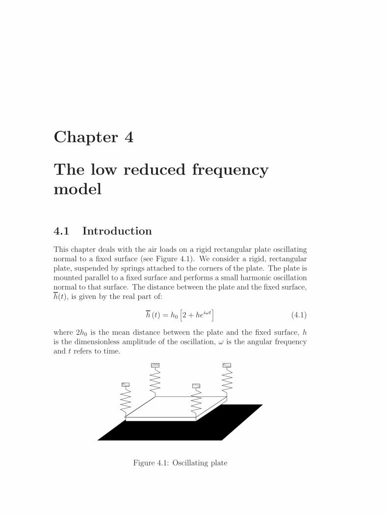
Chapter 4
The low reduced frequencymodel
4.1 Introduction
This chapter deals with the air loads on a rigid rectangular plate oscillatingnormal to a fixed surface (see Figure 4.1). We consider a rigid, rectangularplate, suspended by springs attached to the corners of the plate. The plate ismounted parallel to a fixed surface and performs a small harmonic oscillationnormal to that surface. The distance between the plate and the fixed surface,h(t), is given by the real part of:
h (t) = h0
[2 + heiωt
](4.1)
where 2h0 is the mean distance between the plate and the fixed surface, his the dimensionless amplitude of the oscillation, ω is the angular frequencyand t refers to time.
Figure 4.1: Oscillating plate
60 The low reduced frequency model
The plate is assumed to be rigid. Hence, any uncertainty with respect tothe dynamical behaviour of the plate is excluded. The forces acting on theplate due to the pressure distribution in the gap will affect the eigenfrequencyand the damping of the system. The airloads can thus be determined bymeasuring the eigenfrequency and the damping of the system.
For the behaviour of the air in the gap between the plate and the fixedsurface an analytical solution is presented, based on a low reduced frequencymodel. As a first check, the results from the analytical solution are comparedwith the results from a standard finite element technique, based on the waveequation. In these calculations the air is represented as a compressible, in-viscid medium. The analytical solution is validated with specially designedexperiments.
Most of the experiments described in the literature are carried out atrelatively high frequencies. In order to obtain low shear wave numbers, verysmall gaps widths were used. For these gap widths low damping levels in thefrequency range of interest were found. However, such a small gap width isdifficult to control and consequently the accuracy of the results is often notvery clear. A further drawback is the fact that the amplitude of oscillationhas to be kept very small in order to avoid non-linearities. Finally, mostexperiments were carried out with relatively heavy structural materials. Forsuch materials the air loads have a small influence on the dynamical behaviourof the system. Consequently the frequency shifts and the damping values arenot very large.
The experimental setup, presented in this chapter, was specially designedto avoid many of these problems. With the help of the aforementioned di-mensionless parameters a large scale setup was constructed. Typical prop-erties of the setup are: plate dimensions 0.98 x 0.98 m2, plate mass 2.54 kg,gap widths from 3 to 650 mm. The eigenfrequency of the single degree offreedom mass-spring system in vacuum is 9.73 Hz. The frequency range ofinterest is the range from 1 to 10 Hz. The plate is excited in the centre by anelectrodynamic shaker. Because of the fact that the panel is very light, thefrequency shift and the amount of damping are very large. The large scale ofthe setup makes it possible to measure the pressure distribution in the gap.This provides new information regarding the accuracy of the models and theboundary conditions.

4.2 Analytical calculations 61
4.2 Analytical calculations
4.2.1 Pressure distribution
The low reduced frequency equation for this geometry is (see chapter 2 andAppendix B):
∂2p
∂x2+∂2p
∂y2− Γ2p = n(sσ)Γ2 1
2h (4.2)
where the functions B(s) and n(sσ) are given by:
B(s) =tanh
(s√i)
s√i
− 1 ; n (sσ) =
[1 +
[γ − 1
γ
]B (sσ)
]−1
(4.3)
The boundary conditions are:
p = 0 for x = ±kx ; p = 0 for y = ±akx (4.4)
where kx is a wave number and a is the aspect ratio of the plate:
kx =ωlxc0
; a =lylx
(4.5)
The applied boundary condition is p = 0 (see Figure 4.2). This is a simplifi-cation, since the pressure distribution outside the gap will be affected by thepressure distribution in the gap and vice versa. For narrow gaps, however,the magnitude of the pressure perturbation in the gap is very large com-pared to the magnitude of the pressure perturbation outside the gap. Hence,the boundary condition p = 0 is a realistic assumption. This is confirmedby straightforward potential flow calculations, a comparison with finite ele-ment results and experimental results. A more extensive discussion on thisboundary condition is given in the sections 4.3 and 4.5.3.
Plate
Fixed surface p=0 p=0Air gap
Figure 4.2: Boundary conditions for the analytical model
The solution for the pressure is:
p(x, y) =2n(sσ)Γ2k2
xh
π
∑q=1,3,5···
(−1)q−1
2
qD2
cosh(D 1
kxx)
cosh (D)− 1
cos(qπ
2
1
akxy)
(4.6)
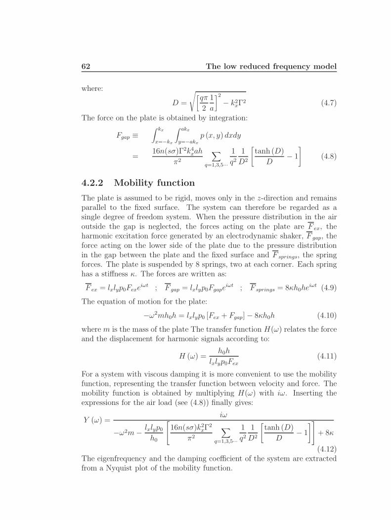
62 The low reduced frequency model
where:
D =
√[qπ
2
1
a
]2
− k2xΓ
2 (4.7)
The force on the plate is obtained by integration:
Fgap ≡∫ kx
x=−kx
∫ akx
y=−akxp (x, y) dxdy
=16n(sσ)Γ2k4
xah
π2
∑q=1,3,5···
1
q2
1
D2
[tanh (D)
D− 1
](4.8)
4.2.2 Mobility function
The plate is assumed to be rigid, moves only in the z-direction and remainsparallel to the fixed surface. The system can therefore be regarded as asingle degree of freedom system. When the pressure distribution in the airoutside the gap is neglected, the forces acting on the plate are F ex, theharmonic excitation force generated by an electrodynamic shaker, F gap, theforce acting on the lower side of the plate due to the pressure distributionin the gap between the plate and the fixed surface and F springs, the springforces. The plate is suspended by 8 springs, two at each corner. Each springhas a stiffness κ. The forces are written as:
F ex = lxlyp0Fexeiωt ; F gap = lxlyp0Fgape
iωt ; F springs = 8κh0heiωt (4.9)
The equation of motion for the plate:
−ω2mh0h = lxlyp0 [Fex + Fgap]− 8κh0h (4.10)
where m is the mass of the plate The transfer function H(ω) relates the forceand the displacement for harmonic signals according to:
H (ω) =h0h
lxlyp0Fex(4.11)
For a system with viscous damping it is more convenient to use the mobilityfunction, representing the transfer function between velocity and force. Themobility function is obtained by multiplying H(ω) with iω. Inserting theexpressions for the air load (see (4.8)) finally gives:
Y (ω) =iω
−ω2m− lxlyp0
h0
16n(sσ)k2xΓ
2
π2
∑q=1,3,5···
1
q2
1
D2
[tanh (D)
D− 1
]+ 8κ
(4.12)The eigenfrequency and the damping coefficient of the system are extractedfrom a Nyquist plot of the mobility function.
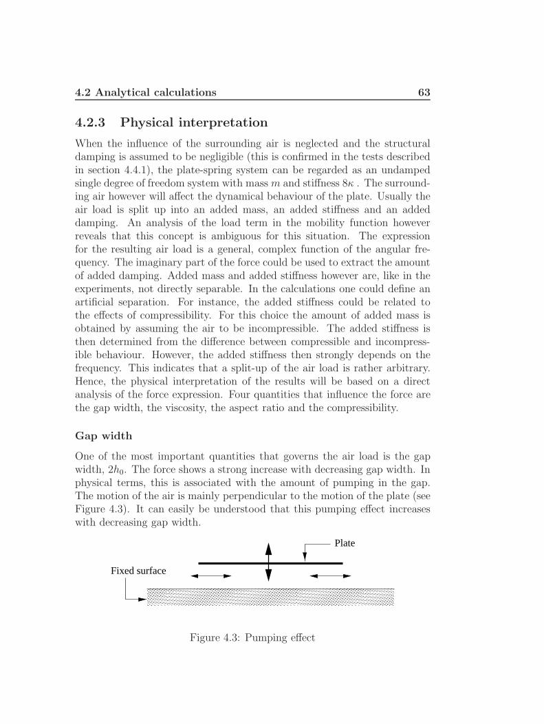
4.2 Analytical calculations 63
4.2.3 Physical interpretation
When the influence of the surrounding air is neglected and the structuraldamping is assumed to be negligible (this is confirmed in the tests describedin section 4.4.1), the plate-spring system can be regarded as an undampedsingle degree of freedom system with mass m and stiffness 8κ . The surround-ing air however will affect the dynamical behaviour of the plate. Usually theair load is split up into an added mass, an added stiffness and an addeddamping. An analysis of the load term in the mobility function howeverreveals that this concept is ambiguous for this situation. The expressionfor the resulting air load is a general, complex function of the angular fre-quency. The imaginary part of the force could be used to extract the amountof added damping. Added mass and added stiffness however are, like in theexperiments, not directly separable. In the calculations one could define anartificial separation. For instance, the added stiffness could be related tothe effects of compressibility. For this choice the amount of added mass isobtained by assuming the air to be incompressible. The added stiffness isthen determined from the difference between compressible and incompress-ible behaviour. However, the added stiffness then strongly depends on thefrequency. This indicates that a split-up of the air load is rather arbitrary.Hence, the physical interpretation of the results will be based on a directanalysis of the force expression. Four quantities that influence the force arethe gap width, the viscosity, the aspect ratio and the compressibility.
Gap width
One of the most important quantities that governs the air load is the gapwidth, 2h0. The force shows a strong increase with decreasing gap width. Inphysical terms, this is associated with the amount of pumping in the gap.The motion of the air is mainly perpendicular to the motion of the plate (seeFigure 4.3). It can easily be understood that this pumping effect increaseswith decreasing gap width.
Fixed surface
Plate
Figure 4.3: Pumping effect

64 The low reduced frequency model
Viscosity
A very interesting point is the role of the viscosity. The viscosity affects boththe real and the imaginary part of the propagation constant Γ. The dampingdepends on the viscosity, as expected. However, the eigenfrequency of thesystem is also affected by the viscosity. In this investigation the phase reso-nance frequency is used: the eigenfrequency of the corresponding undampedsystem. Therefore the eigenfrequency is, by definition, not influenced by thedamping. The eigenfrequency shift due to viscosity may thus seem surpris-ing. Simply speaking one would expect the viscosity to affect the damping,but not the eigenfrequency. The change in frequency can be attributed tothe change in the velocity profile in the gap. For low shear wave numbersthere is a parabolic profile, whereas for high shear wave numbers the velocityprofile is flat (see section 2.5.3). It is therefore important that, for a correctestimation of the eigenfrequency, the viscosity is taken into account.
Compressibility
In the calculations one can easily eliminate the effects of the compressibility.For incompressible behaviour, the function D (see expression (4.7)), reducesto:
Dinc =qπ
2
1
a(4.13)
Compressibility effects are important when:
|kxΓ| ∼=(π
2
)(1
a
)(4.14)
This can be rewritten to: ∣∣∣∣∣ ωlyceff(ω)
∣∣∣∣∣ ∼= π
2(4.15)
where ceff(ω) is an effective speed of sound:
ceff(ω) =ic0
Γ(4.16)
The effective speed of sound is affected by viscous effects and thermal effects.In physical terms, expression (4.15) now simply states that compressibilityeffects are important when the effective acoustic wavelength is of the sameorder of magnitude as the plate length.

4.3 Standard acoustic finite element calculations 65
4.3 Standard acoustic finite element calcula-
tions
As a first check, the results from the analytical solution with the results froma standard finite element technique, based on the wave equation. In thesecalculations the air is represented as a compressible, inviscid medium. Thefinite element calculations were carried out for the experimental setup (seesection 4.4.1) with the program ANSYS [81]. A rectangular solar panel issuspended by 8 springs, two at each corner. The panel has a mass m and(equivalent) Young’s modulus E; each spring has a stiffness κ. The thicknessof the panel is 0.022 m. The plate is modelled as an elastic body. Thedeformation of the plate however is shown to be small in the frequency rangeof interest (see also section 4.4.4). This frequency range is far below the firstelastic eigenfrequency of the panel. The gap width between the plate and thefixed surface can be varied between 2 and 650 mm. The following propertiesare taken according to the measurements 1:
m = 2.540 kg ; κ = 1186 N/m
lx = 0.49 m ; ly = 0.49 m (4.17)
E = 2.61 · 109 N/m2
The properties of the surrounding air at standard atmospheric conditions:
ρ0 = 1.2 kg/m3 ; c0 = 343 m/s (4.18)
The panel is modelled with three-dimensional 8-node solid elements, typeSOLID45. The degrees of freedom at each node are the displacements. InANSYS the air is represented as a compressible, inviscid medium. Thebehaviour of the air is therefore governed by the wave equation. Three-dimensional 8-node acoustic elements, type FLUID30 , were used. For theacoustic elements, the pressure perturbation is the degree of freedom at eachnode. With the use of symmetry the mesh is reduced to 1/4 of the system (seeFigure 4.4). In the numerical calculations, the two springs at each corner arereplaced by a single spring with a double stiffness. The boundary conditionfor the pressure on the planes of symmetry and the fixed surface is that thepressure gradient normal to the wall should vanish. In physical terms, thiscondition states that the velocity of the air normal to the surface is equal tozero. This condition is automatically satisfied in the ANSYS program whenno other boundary conditions are specified.
1The mass of the panel includes the mass of some instrumentation. Young’s modulusis an equivalent quantity for the layered honeycomb panel.

66 The low reduced frequency model
pn
δδδ
δ =0
l =
pn
δ
δ
surface
Plate
Symmetryplane
Fixed
0.49 m
p=0
x
2h0
=0
p=0
1.49 m
1.42
5 m
Figure 4.4: Finite element mesh
The boundary condition for the other air boundaries is p = 0. This isa simplification of the Sommerfeld radiation condition, which states that allwaves are outgoing. The condition p = 0 however will give reliable resultswhen the dimensions of the surrounding air domain are sufficiently large(without introducing standing waves). As a test case, the added mass wascalculated for an oscillating plate in an infinite air domain for a number ofmesh dimensions. The results showed that for an air domain of 1.49 x 1.49(in-plane) x 1.425 m3 (perpendicular to the plate), the added mass differsonly by 3.8% from the value given in the literature [82]. This justifies theuse of the boundary condition p = 0 for the finite element calculations. Notethat the influence of the air on the upper side of the panel is also accountedfor in the finite element model. The accuracy of the p = 0 condition, used inthe analytical model at the edges of the panel, can be investigated with thismodel where also (part of) the surrounding air is taken into account. Theresults for the pressure distribution will be compared with experimental andanalytical results.
4.4 Experiments
4.4.1 Experimental setup
In order to measure the effects of the surrounding air, a relatively light andstiff plate must be used. A solar panel is very well suited for this purpose.The measurements were carried out using a square ECS panel (courtesy ofFokker Space & Systems) of 0.98 x 0.98 m2. The panel consists of 2 carbon
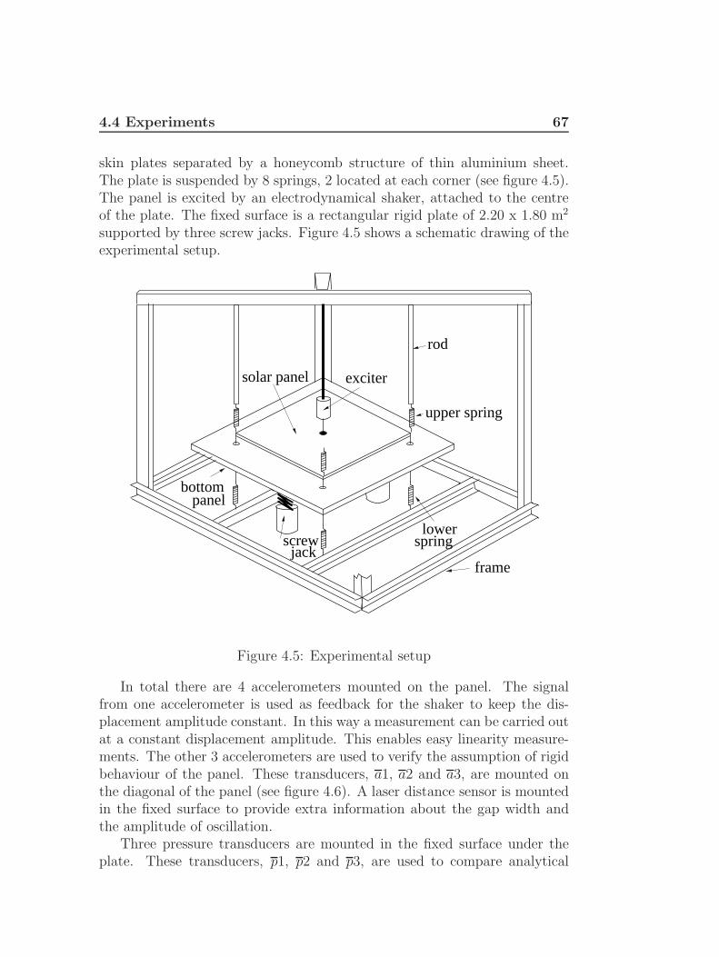
4.4 Experiments 67
skin plates separated by a honeycomb structure of thin aluminium sheet.The plate is suspended by 8 springs, 2 located at each corner (see figure 4.5).The panel is excited by an electrodynamical shaker, attached to the centreof the plate. The fixed surface is a rectangular rigid plate of 2.20 x 1.80 m2
supported by three screw jacks. Figure 4.5 shows a schematic drawing of theexperimental setup.
frame
bottompanel
screwjack
lowerspring
solar panel exciter
rod
upper spring
Figure 4.5: Experimental setup
In total there are 4 accelerometers mounted on the panel. The signalfrom one accelerometer is used as feedback for the shaker to keep the dis-placement amplitude constant. In this way a measurement can be carried outat a constant displacement amplitude. This enables easy linearity measure-ments. The other 3 accelerometers are used to verify the assumption of rigidbehaviour of the panel. These transducers, a1, a2 and a3, are mounted onthe diagonal of the panel (see figure 4.6). A laser distance sensor is mountedin the fixed surface to provide extra information about the gap width andthe amplitude of oscillation.
Three pressure transducers are mounted in the fixed surface under theplate. These transducers, p1, p2 and p3, are used to compare analytical

68 The low reduced frequency model
and numerical data with experimental pressure data. The transducer p3is mounted at the edge of the gap. In this way the validity of the p = 0boundary condition is investigated (see Figure 4.6).
yy
p1 x
a3
a2
a1
0.490
xp2 p3
0.245
Figure 4.6: Instrumentation, dimensions in m.
The undamped eigenfrequency fn (phase resonance frequency), the cor-responding damping coefficient, the accelerations and the atmospheric con-ditions are registered. The properties of interest are 2:
m = 2.540 kg ; R0 = 287 J/kgK
lx = 0.49 m ; ly = 0.49 m
Cp = 1004 J/kgK ; Cv = 716 J/kgK (4.19)
ρ0 = 1.2 kg/m3 ; c0 = 343 m/s
λ = 25.6 · 10−3 W/mK ; µ = 18.2 · 10−6 Ns/m2
κ = 1186 N/m ; T0 = 290 K
4.4.2 Dimensionless parameters
The experimental setup is characterized by the value of the dimensionlessparameters. The main parameter governing the motion of the air in thegap is the shear wave number. For large gaps the viscosity of the air canbe neglected, whereas for small gaps viscous effects become dominant. Thedistance between the panel and the fixed surface, 2h0, can be varied from 2 to650 mm. For this range of gap widths the shear wave number varies between0.64 and 667. As σ is a constant for air, the product sσ varies between 0.4 and520. This implies that for narrow gaps the process in the gap is isothermal,while for large gaps it occurs adiabatically. These considerations indicatethat even for a relatively large gap, e.g. 2 mm, the shear wave number is
2For these conditions σ ∼=√
0.71

4.4 Experiments 69
very low. It should be noted that by varying the gap width not only thevalue of the shear wave number is affected. Another important parameter,the reduced frequency k, varies between 10−5 and 0.06; the condition k 1is therefore satisfied.
4.4.3 Validation of the measurement procedure
The experimental setup was used to measure the shift in eigenfrequencyand the damping originating from the pressure distribution in the gap. Themeasurement procedure was validated by adding a known mass to the paneland to demonstrate that this extra mass can be determined accurately withthe present measuring technique. The shift in phase resonance frequency wasmeasured and used to determine the added mass. The measurement resultsfor two different gap widths are listed in Table 4.1. The Table shows that theadded mass was measured within 3% of the actual, manually added, mass.Hence, it can be concluded that the setup is suited for the measurements inthis investigation.
Measured added mass (kg)Added mass (kg) 2h0 = 650 mm 2h0 = 35 mm
0.0604 0.0605 0.06030.1208 0.1181 0.12200.1816 0.1766 0.18480.2420 0.2348 0.2436
Table 4.1: Validation procedure, measurement results
4.4.4 Accuracy of the measurements
The accuracy of the experiments is affected by several mechanisms. In orderto determine the accuracy of the results, a number of tests were carried out.
Parasitic oscillations
Parasitic oscillations will affect the dynamical behaviour of the system. Inorder to determine whether any parasitic motions were present, accelerationsof the panel and the frame were measured in several directions. Two parasiticoscillations, an in-plane motion of the plate and a frame vibration, were

70 The low reduced frequency model
identified. Some simple structural modifications were applied such that theparasitic motions were eliminated.
Deformation of the panel
Another oscillation that might affect the accuracy of the results is the de-formation of the panel. The first elastic eigenfrequency of the panel in air is49 Hz. In order to consider the panel as rigid, the frequency range of inter-est should be far below 49 Hz. The stiffness of the springs is such that thefirst eigenfrequency of the plate-spring system in vacuum is 9.73 Hz. Due tothe influence of the surrounding air, the eigenfrequency will decrease com-pared to the situation in vacuum. The frequency range of interest thereforewas chosen 1 to 10 Hz, and the panel was assumed to be rigid. During theexperiments, the deformation of the plate was measured. With three ac-celerometers mounted on the plate, the accelerations were measured to checkthat the plate was indeed behaving in a rigid way.
The influence of the deformation of the panel was taken into account in thefinite element calculations. In these calculations the panel was modelled as anelastic body. The results indicate that the influence of the elasticity is small.For a gap width of 150 mm the difference in eigenfrequency between a rigidmodel and a flexible finite element model was less than 0.3 Hz. The differencedecreased as the gap width decreased. Thus, the influence of the elasticitywas small. This was confirmed by the accelerometer data: accelerations ofthe points differ mutually by 4% at most, which justifies the assumption ofrigidity.
Compliance of the fixed surface
The compliance of the fixed surface was measured using the accelerometers.The measurements show that the amplitude of oscillation for the fixed surfaceis less than 1% of the amplitude of oscillation of the panel. The fixed surfacewas therefore regarded as rigid and fixed.
Tilting of the fixed surface
In order to determine the influence of tilting, measurements were carried outfor small tilting angles. For gap widths of 35, 10 and 6 mm. tilting anglesof 1.2, 0.2 and 0.2 degrees respectively were used. For the panel of interest,with a length of 0.98 m, this corresponds to a variation in gap width of 20,4 and 4 mm respectively. The results show that the added mass and theadded damping differred less than 5% for these tilting angles. Because of the

4.4 Experiments 71
fact that global quantities (eigenfrequency and damping) were measured, thesensitivity for small tilting angles was limited.
Curvature of the panel and the fixed surface
The most important quantity that governs the accuracy of the experimentalresults is the gap width. Due to the shape of both the panel and the fixedsurface the accuracy is affected.
The deformation of the fixed surface due to its own weight was calculatedwith a finite element model. A simple static calculation showed that thedeformation due to this dead load is smaller than 0.06 mm. The eigenfre-quencies of the fixed surface were calculated from a dynamic analysis. Alleigenfrequencies were substantially higher than the frequency range of inter-est.
For a certain gap width the distance between the panel and the fixedsurface was measured at 49 points between the panel and the fixed surface.The gap width was not constant but varied with position: ± 0.8 mm. Thiscould mainly be attributed to the planarity of the fixed surface. With a leastsquares technique the accuracy was improved. The gap width data was usedto find the position of the fixed surface that would lead to the best constantgap width in a least squares sense. The gap width was then correspondinglyadjusted in three points for each measurement. Due to this correction, theerror introduced by the planarity of the surfaces could be reduced to ± 0.4mm in gap width.
The influence of the remaining curvature profile was investigated by meansof a special finite element model in the program B2000 3. In this model theviscothermal and acousto-elastic effects are accounted for. Viscothermal ele-ments can be coupled to structural elements. The gap width can be specifiedfor each viscothermal element and elements with different gap widths canbe coupled. In the calculations the measured curvature profile was used tospecify the gap width for each element. The eigenfrequency of the systemwas calcululated. The results indicate that the remaining curvature of thesurfaces has a very small influence: for gap widths between 3 and 35 mm thedifference in eigenfrequency between a flat and a curved model is less than1%. Regarding these considerations, the measurements could be carried outwith a satisfying accuracy, especially compared to previous papers in thisarea.
3A detailed description of this model is given in chapter 5

72 The low reduced frequency model
Non-linear effects
The theory used in the present investigation is based on linearized equations.In the experiments the amplitude of oscillation of the panel therefore mustbe small compared to the gap width. In order to determine whether anynon-linear effects are present a number of experiments were carried out withdifferent amplitudes of oscillation. For several gap widths measurements wereperformed at several amplitude levels. In all situations, the eigenfrequencyand the damping were not affected by the amplitude of motion.
Flow around plate edges
The flow around the plate edges was visualized with smoke tests. In thefrequency and amplitude ranges of interest, no irregularities or disturbancesin the flow pattern were observed.
Reproducibility
The measurement series was repeated a number of times to investigate thereproducibility of the experiments. The results show that the reproducibilitywas very good. Data of the measurement series are given in Appendix D.
4.4.5 Experimental results
Typical results for the transfer function are presented in Figure 4.7. ThisFigure shows that the shift in eigenfrequency is relatively large. If one con-verts this frequency shift to an added mass for a gap of 3 mm, the amountof added mass amounts to about 22 kg, while the mass of the panel is only2.5 kg! The sharp increase in damping is illustrated by the flattening of thetransfer function. The pumping effect induces high viscous losses, which re-sults in damping of the panel. For a gap of 3 mm, the dimensionless dampingcoefficient ξ is 35%: the panel is almost critically damped. The experimentalresults are summarized in Table 4.2. For each gap width the eigenfrequency,the damping coefficient and the dimensionless parameters are listed.
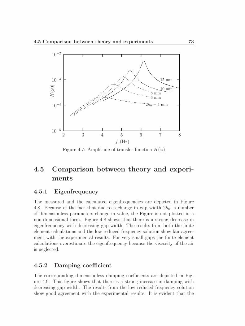
4.5 Comparison between theory and experiments 73
2h0 = 4 mm
6 mm8 mm
10 mm
15 mm
f (Hz)
|H(ω
)|
8765432
10−2
10−3
10−4
10−5
Figure 4.7: Amplitude of transfer function H(ω)
4.5 Comparison between theory and experi-
ments
4.5.1 Eigenfrequency
The measured and the calculated eigenfrequencies are depicted in Figure4.8. Because of the fact that due to a change in gap width 2h0, a numberof dimensionless parameters change in value, the Figure is not plotted in anon-dimensional form. Figure 4.8 shows that there is a strong decrease ineigenfrequency with decreasing gap width. The results from both the finiteelement calculations and the low reduced frequency solution show fair agree-ment with the experimental results. For very small gaps the finite elementcalculations overestimate the eigenfrequency because the viscosity of the airis neglected.
4.5.2 Damping coefficient
The corresponding dimensionless damping coefficients are depicted in Fig-ure 4.9. This figure shows that there is a strong increase in damping withdecreasing gap width. The results from the low reduced frequency solutionshow good agreement with the experimental results. It is evident that the
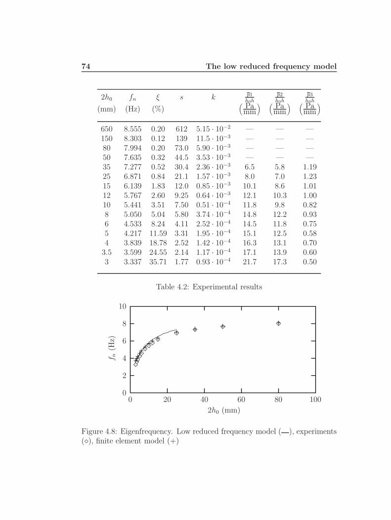
74 The low reduced frequency model
2h0 fn ξ s k p1h0h
p2h0h
p3h0h
(mm) (Hz) (%)(
Pamm
) (Pamm
) (Pamm
)650 8.555 0.20 612 5.15 · 10−2 — — —150 8.303 0.12 139 11.5 · 10−3 — — —80 7.994 0.20 73.0 5.90 · 10−3 — — —50 7.635 0.32 44.5 3.53 · 10−3 — — —35 7.277 0.52 30.4 2.36 · 10−3 6.5 5.8 1.1925 6.871 0.84 21.1 1.57 · 10−3 8.0 7.0 1.2315 6.139 1.83 12.0 0.85 · 10−3 10.1 8.6 1.0112 5.767 2.60 9.25 0.64 · 10−3 12.1 10.3 1.0010 5.441 3.51 7.50 0.51 · 10−4 11.8 9.8 0.828 5.050 5.04 5.80 3.74 · 10−4 14.8 12.2 0.936 4.533 8.24 4.11 2.52 · 10−4 14.5 11.8 0.755 4.217 11.59 3.31 1.95 · 10−4 15.1 12.5 0.584 3.839 18.78 2.52 1.42 · 10−4 16.3 13.1 0.70
3.5 3.599 24.55 2.14 1.17 · 10−4 17.1 13.9 0.603 3.337 35.71 1.77 0.93 · 10−4 21.7 17.3 0.50
Table 4.2: Experimental results
2h0 (mm)
f n(H
z)
100806040200
10
8
6
4
2
0
Figure 4.8: Eigenfrequency. Low reduced frequency model ( ), experiments(), finite element model (+)

4.5 Comparison between theory and experiments 75
damping coefficients for the finite element calculations are zero, because thedissipative effects are neglected.
2h0 (mm)
ξ(%
)
50454035302520151050
40
35
30
25
20
15
10
5
0
Figure 4.9: Damping coefficient. Low reduced frequency model ( ), experi-ments ()
4.5.3 Pressure
The pressure in the layer was measured at three points as a function of the gapwidth 2h0 (see Figure 4.6). Since the pressure in the layer is also frequencydependent, the amplitude of the pressure was measured at the eigenfrequencyfor each gap width. The maximum pressure was scaled with the displacementamplitude h0h. The results from the calculations and the measurements aregiven in Figures 4.10, 4.11 and 4.12. In order to investigate the influence ofviscous and thermal effects the analytical low reduced frequency results arealso given where viscous and thermal effects were eliminatedby setting Γ = iand n(sσ) = γ.
For p1 and p2, the pressure shows a strong increase with decreasing gapwidth. All models predict this increase, but the viscothermal model and theexperimental model both show a very strong increase with decreasing gapwidth. Viscothermal effects thus have a significant influence on the pressuredistribution for small gap widths 4.
The results for p3 indicate that the pressure is not zero at the edges of thepanel. For larger gap widths the pressure at the edge is significant comparedto the maximum pressure in the layer. For small gaps however the influence
4Note that the pressure point for 2h0 = 3 mm is significant since it is the result of moremeasurements with good reproducibility

76 The low reduced frequency model
2h0 (mm)
p 1 h0h
( Pa
mm
)
4035302520151050
25
20
15
10
5
0
Figure 4.10: Scaled pressure p1. Low reduced frequency model ( ), inviscidand adiabatic low reduced frequency model (−−) , experiments (), ANSYSfinite element model (+)
2h0 (mm)
p 2 h0h
( Pa
mm
)
4035302520151050
25
20
15
10
5
0
Figure 4.11: Scaled pressure p2. Low reduced frequency model ( ), inviscidand adiabatic low reduced frequency model (−−) , experiments (), ANSYSfinite element model (+)
of the non-zero boundary pressure is small. Since the low reduced frequencymodel is used for small gaps, it can be concluded that the boundary conditionp = 0 is acceptable regarding the balance between simplicity and accuracy.If a more detailed prediction of the pressure at the edges is required, the lowreduced frequency model must be coupled to an acoustic model describingthe behaviour of the surrounding air. The standard acoustic finite element

4.5 Comparison between theory and experiments 77
2h0 (mm)
p 3 h0h
( Pa
mm
)
4035302520151050
54.5
43.5
32.5
21.5
10.5
0
Figure 4.12: Scaled pressure p3. Experiments (), ANSYS finite elementmodel (+)
model is able to predict the pressure at the edge to a reasonable degree ofaccuracy. In the next chapter a finite element model is presented for thelow reduced frequency model. This model could be coupled to a standardacoustic model describing the behaviour of the surrounding air.

78 The low reduced frequency model
4.6 Panel rotating around central axis
Experiments and calculations were also carried out for a solar panel rotatingaround a central axis (see Figure 4.13).
Fixed surface p=0
Torsion springPlate
Air gap p=0
Figure 4.13: Panel rotating around y = 0
The panel is located parallel to a fixed surface and performs a smallangular oscillation around y = 0. It is suspended by a torsion spring 5. Thedistance between the plate and the fixed surface is:
h(x, y, t) = h0
[2 + α
(akxk
)yeiωt
](4.20)
where α is the amplitude of the angular oscillation and:
kx =ωlxc0
; a =lylx
(4.21)
For this single degree of freedom system, eigenfrequency and damping werecalculated and measured. The same procedure was used as for the translatingpanel. For the sake of brevity, only the main procedure and the main resultswill be presented.
4.6.1 Analytical calculations
The low reduced frequency equation for this situation is:
∂2p
∂x2+∂2p
∂y2− Γ2p = n(sσ)Γ2 1
2α
(akxk
)y (4.22)
where the functions B(s) and n(sσ) are given by:
B(s) =tanh
(s√i)
s√i
− 1 ; n (sσ) =
[1 +
[γ − 1
γ
]B (sσ)
]−1
(4.23)
5In the experiments these are springs at a certain distance from the axis of rotation

4.6 Panel rotating around central axis 79
Spring
Solar panel
Axis of rotation
Shaker
Figure 4.14: Experimental setup rotating panel
The boundary conditions are:
p = 0 for x = ±kx ; p = 0 for y = ±akx (4.24)
The solution for the pressure is:
p(x, y) =2n(sσ)aΓ2k3
xα
πk
∑q=2,4,6···
(−1)q−1
2
qD2
cosh(D 1
kxx)
cosh (D)− 1
sin(qπ
2
1
akxy)
(4.25)where:
D =
√[qπ
2
1
a
]2
− k2xΓ
2 (4.26)
Clearly, the force exerted on the plate is zero for the rotating panel becauseof the asymmetric pressure distribution. With the pressure distribution, thenet moment acting on the plate around y = 0 was calculated and insertedinto the equation of motion. The mobility function was then constructed andeigenfrequency and damping were extracted.
4.6.2 Experiments
The experiments were carried out with a solar panel of 1.67 x 1.29 m2. Themass moment of inertia of the panel and the instrumentation was 1.64 kgm2.The panel was suspended by 8 springs, 2 located in each of the four pointsat the edges of the panel (see Figure 4.14).
The eigenfrequency of the panel-spring system in vacuum was 2.96 Hz.Due to the influence of the air, the eigenfrequency will be reduced. The fre-quency range of interest therefore is 1 to 3 Hz. Accelerometers were mounted

80 The low reduced frequency model
on the panel to verify the rigidity of the panel. In the mentioned frequencyrange the deformation of the panel was negligible. The panel was excitedwith an electrodynamic shaker. The fixed surface was a rectangular rigidplate of 2.2 x 1.8 m2, which was mounted on a frame parallel to the panel.The distance between the plate and the fixed surface was varied between 3and 50 mm. The shear wave number for this configuration varies between 1.9and 55. This implies that for thin layers the viscous forces are of the sameorder of magnitude as the inertial forces. The properties of the air were takenaccording to expression (4.19). The remaining properties of interest are:
I = 1.64 kgm2 ; κ = 245 N/m
lx = 0.835 m ; ly = 0.645 m
lspr = 0.538 m (4.27)
where I denotes the mass moment of inertia of the pane, κ is the stiffnessof a single spring and lspr denotes the distance between the springs and theaxis of rotation. The measured eigenfrequency and damping coefficient arelisted in Appendix D.
4.6.3 Comparison between theory and experiments
The experimental results and the analytical results are illustrated in Figures4.15 and 4.16.
2h0 (mm)
f n(H
z)
50454035302520151050
3
2.5
2
1.5
1
0.5
0
Figure 4.15: Eigenfrequency. Low reduced frequency model ( ), experi-ments ()
Figure 4.15 shows that the eigenfrequency of the system decreases withdecreasing gap width. For the rotating panel, the shift in eigenfrequency can

4.7 Panel rotating around arbitrary axis 81
2h0 (mm)
ξ(%
)
50454035302520151050
60
50
40
30
20
10
0
Figure 4.16: Damping coefficient. Low reduced frequency model ( ), exper-iments ()
be interpreted as an added mass moment of inertia. For the panel underconsideration, the mass moment of ineria is 1.64 kgm2. For a gap width of3 mm the added mass moment of inertia due to the pressure in the layer is5.5 kgm2. The damping shows a strong increase with decreasing gap width.Calculations and experiments show fair agreement.
4.7 Panel rotating around arbitrary axis
Analytical solutions were obtained for a normal translation of the panel anda central rotation. Because of the linearity of the problem, these solutionscan now be used to calculate the behaviour of a rigid panel rotating aroundan arbitrary axis. Consider for instance a panel rotating around y = ya(see Figure 4.17). The motion can be decomposed into a translation and arotation around y = 0. In the Figure the resulting forces and moments arealso shown. In a similar way, the response for a rotation around an arbitraryaxis can be obtained.

82 The low reduced frequency model
y
α
a
a
Central rotation
Translation
α
α
y
Total motion
M
F
MF
Figure 4.17: Panel rotating around arbitrary axis
4.8 Conclusions
The conclusions to be drawn from this investigation are:
• a special experimental setup was designed to validate the low reducedfrequency model. With the use of the dimensionless parameters a newlarge-scale setup was developed. Substantial frequency shifts, very largedamping values and pressures in the layer were measured with satis-factory accuracy;
• calculations and experiments show fair agreement: the low reducedfrequency model is a satisfactory means to describe viscothermal wavepropagation. The eigenfrequency and damping of the system and thepressure in the layer could be predicted accurately using the low re-duced frequency model.

Chapter 5
Acousto-elasticity:viscothermal finite elements
5.1 Introduction
In chapter 2 an overview was presented of models for viscothermal wavepropagation. It was demonstrated that the low reduced frequency model isa very simple and useful model. In chapter 4 this model was experimentallyvalidated for a vibrating rigid surface. In view of practical applications,however, it is important to develop models that include the acousto-elasticinteraction between flexible surfaces and viscothermal gas layers. Analyticalsolutions can only be obtained for simple geometries with simple boundaryconditions.
This chapter describes the development, implementation and analyticaland experimental validation of a new finite element model. The finite ele-ment model enables the modelling of more complex geometries and boundaryconditions. In chapter 6 this model will be used for a number of practicalapplications.
5.2 Finite element formulation
The starting point for the new acoustic finite element is the low reducedfrequency equation (see equation (2.28)):
∆pdp(xpd
)− k2Γ2p
(xpd
)= −ikn(sσ)Γ2< (5.1)
In dimensional form, dropping the (xpd) notation:
∆pdp− ω2Γ2
c20
p = −ikn(sσ)Γ2ρ0c20
l2γ< (5.2)

84 Acousto-elasticity: viscothermal finite elements
This equation is multiplied by a weighting function ww and integrated over
the volume. The volume integral can be split up in an integration over Acd
and Apd
. For layer geometries Acd
is the thickness of the layer and Apd
is
the total area of the squeezing surfaces. For tube geometries, Acd
is the
cross-sectional area of the tube and Apd
is the axial direction. This meansthat, depending on the type of geometry, integration over A
cd(layers) or
Apd
(tubes) actually is a line integration. In Appendix B a more detaileddescription is given for each geometry.∫
Acd
∫Apdww
[∆pdp− ω2Γ2
c20
p+ikn(sσ)Γ2ρ0c
20
l2γ<]dA
pddA
cd= 0 (5.3)
The integrand is not a function of the cd-co-ordinates. The integration over
Acd
is carried out to enable coupling between elements with different cross-sectional areas and to enable coupling with standard acoustic finite elements,see section 5.3. Using Green’s theorem and partial integration:
Acd∫∂A
pdww∇pd
p · en d∂Apd − Acd
∫Apd∇pd
ww · ∇pdp dA
pd+
− ω2Γ2
c20
Acd∫Apdwwp dA
pd+
+ikn(sσ)Γ2ρ0c
20
γl2Acd∫Apdww< dApd = 0 (5.4)
where ∂Apd
is the boundary of Apd
. Inserting the expression for <, seeexpression (2.29), and relating the acoustic velocity v on the interface to thestructural displacement us, (v = iω
c0us), gives:
Acd∫∂A
pdww∇pd
p · en d∂Apd − Acd
∫Apd∇pd
ww · ∇pdp dA
pd+
− ω2Γ2
c20
Acd∫Apdwwp dA
pd+ (5.5)
− ρ0ω2n(sσ)Γ2
γl
Acd
Acd
∫Apd
∫∂Acd
wwus · en d∂Acd dApd
= 0
The pressure in each element is expressed in terms of the interpolation func-tions [Na] and the nodal pressures P. The structural displacement is alsowritten in terms of interpolation functions:
p = [Na] P ; us = [Ns] U (5.6)
Following Galerkin’s approach, the weighting functions are chosen equal tothe interpolation functions. For an acoustic hard wall, the normal derivative

5.2 Finite element formulation 85
of the pressure is zero. In the case of a prescribed pressure the weightingfunction is chosen equal to zero. The first term only contributes for animpedance-like boundary condition. However, one has to bear in mind thatthe pressure is constant across the gap width or cross section, while the in-plane velocities (layer geometry) or the axial velocity (tube geometry) vary.An impedance can therefore only be defined in an integrated sense. The termwith the normal derivative of the pressure is set equal to zero in the presentstudy. This finally leads to the following set of equations:
−ω2 [Ma(s)] P+ [Ka] P = ω2 [M c(s)] U (5.7)
where [Ma (s)] denotes the acoustic mass matrix, [Ka] is the acoustic stiffnessmatrix, P is the vector with the nodal pressure degrees of freedom, U isthe vector with the nodal structural degrees of freedom and [Mc (s)] is thecoupling matrix. Their elements are given by:
[Ma (s)] = −Γ2
c20
Acd∫Apd
[Na]T · [Na] dApd
(5.8)
[Ka] = Acd∫Apd
[∇pd
Na]T·[∇pd
Na]dA
pd(5.9)
[M c (s)] = −ρ0n(sσ)Γ2
γl
Acd
Acd
∫Apd
∫∂Acd
[Na]T · [en ·Ns] d∂Acd dApd
(5.10)
Because the propagation constant Γ is complex and depends on the shearwave number, the acoustic mass matrix is also complex and shear wave num-ber, e.g. frequency, dependent. In fact, the mass matrix is equal to the corre-sponding standard acoustic mass matrix, only it is premultiplied by −Γ2/c2
0
instead of 1/c20. The finite element model for the structure, in the absence of
structural damping, can be written in the following standard formulation:
−ω2 [Ms] U + [Ks] U = [Kc] P+F ext
(5.11)
where [Ms] denotes the structural mass matrix, [Ks] is the stiffness matrix,[Kc] is the coupling matrix resulting from the pressure on the interface andF ext is the external nodal force vector. The principle of virtual work givesthe following expression for the coupling matrix [Kc] :
[Kc (s)] =∂A
cd
∂Acd
∫Apd
∫∂Acd
[en ·Ns]T · [Na] d∂Acd dApd
(5.12)
The acousto-elastic interaction is established by demanding continuity ofnormal velocity across the interface. This now gives the following coupled
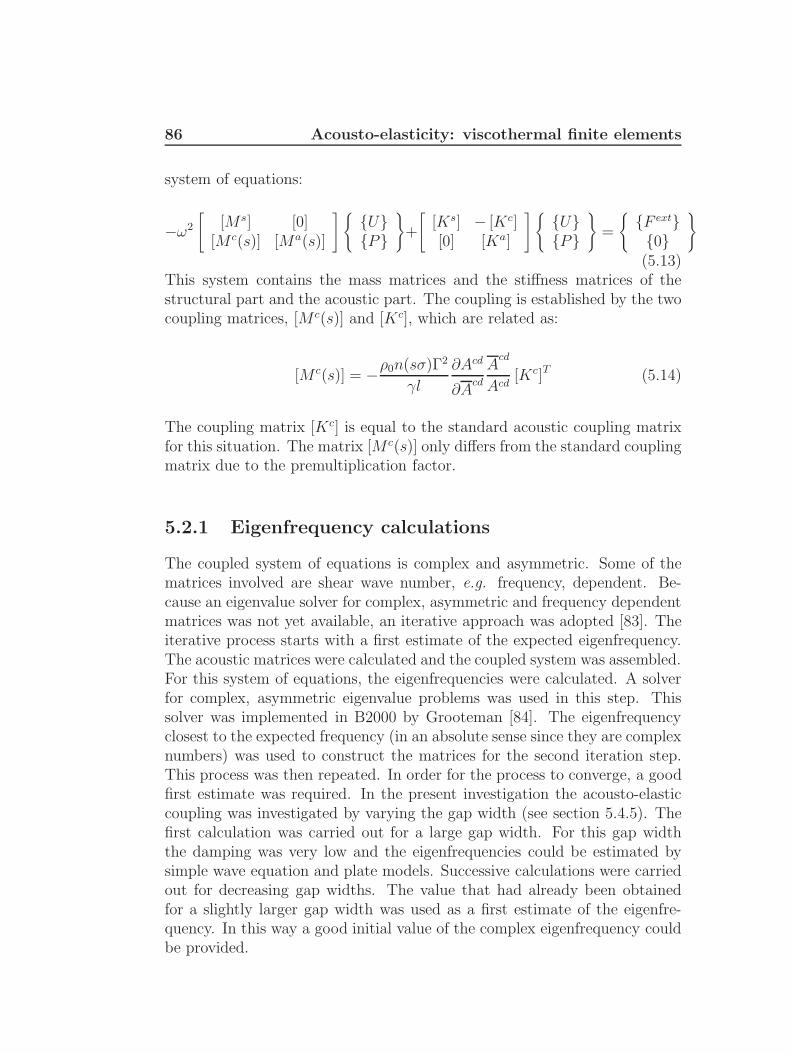
86 Acousto-elasticity: viscothermal finite elements
system of equations:
−ω2
[[Ms] [0]
[M c(s)] [Ma(s)]
]UP
+
[[Ks] − [Kc][0] [Ka]
]UP
=
F ext0
(5.13)
This system contains the mass matrices and the stiffness matrices of thestructural part and the acoustic part. The coupling is established by the twocoupling matrices, [M c(s)] and [Kc], which are related as:
[M c(s)] = −ρ0n(sσ)Γ2
γl
∂Acd
∂Acd
Acd
Acd[Kc]T (5.14)
The coupling matrix [Kc] is equal to the standard acoustic coupling matrixfor this situation. The matrix [M c(s)] only differs from the standard couplingmatrix due to the premultiplication factor.
5.2.1 Eigenfrequency calculations
The coupled system of equations is complex and asymmetric. Some of thematrices involved are shear wave number, e.g. frequency, dependent. Be-cause an eigenvalue solver for complex, asymmetric and frequency dependentmatrices was not yet available, an iterative approach was adopted [83]. Theiterative process starts with a first estimate of the expected eigenfrequency.The acoustic matrices were calculated and the coupled system was assembled.For this system of equations, the eigenfrequencies were calculated. A solverfor complex, asymmetric eigenvalue problems was used in this step. Thissolver was implemented in B2000 by Grooteman [84]. The eigenfrequencyclosest to the expected frequency (in an absolute sense since they are complexnumbers) was used to construct the matrices for the second iteration step.This process was then repeated. In order for the process to converge, a goodfirst estimate was required. In the present investigation the acousto-elasticcoupling was investigated by varying the gap width (see section 5.4.5). Thefirst calculation was carried out for a large gap width. For this gap widththe damping was very low and the eigenfrequencies could be estimated bysimple wave equation and plate models. Successive calculations were carriedout for decreasing gap widths. The value that had already been obtainedfor a slightly larger gap width was used as a first estimate of the eigenfre-quency. In this way a good initial value of the complex eigenfrequency couldbe provided.

5.2 Finite element formulation 87
5.2.2 Frequency response calculations
A frequency response calculation can be carried out by solving the coupled setof equations (5.13) for a given excitation and frequency. The frequency de-pendence of the matrices complicates such a frequency response calculation.However, the special structure of the matrices allows for a very straight-forward and elegant way of reducing the computational efforts: componentmode synthesis. The coupled viscothermal response can be expressed interms of the uncoupled inviscid, adiabatic acoustic modes and the uncou-pled structural modes. Consider the acousto-elastic model for the inviscid,adiabatic case:
−ω2
[[Ms] [0][M c
] [Ma
] ] UP
+
[[Ks] − [Kc][0] [Ka]
]UP
=
F ext0
(5.15)
where[M c
]and
[Ma
]are the matrices for the inviscid, adiabatic case. These
matrices are obtained by simply setting Γ = i and n(sσ) = γ in the expres-sions for the low reduced frequency model. The uncoupled acoustic modesfor this situation are calculated from (
[Ka]
= [Ka]):
−ω2[Ma(s)
]P+ [Ka] P = 0 (5.16)
The eigenmodes are stored (columnwise) in the matrix[Φa]
and the acousticeigenvalues, i.e. the squares of the angular frequencies, are stored in thematrix
[Ωa]. The modes are normalized with respect to the acoustic mass
matrix: [Φa]T [
Ma] [
Φa]
= [I] ;[Φa]T
[Ka][Φa]
=[Ωa]
(5.17)
Calculation of the acoustic eigenmodes and eigenfrequencies is very straight-forward and efficient. For layer geometries the problem is 2-dimensional,while for tube geometries the problem is only 1-dimensional. All matricesinvolved are real valued. The uncoupled structural modes are obtained from:
−ω2 [Ms] U+ [Ks] U = 0 (5.18)
The structural eigenmodes are stored (columnwise) in the matrix [Φs] andthe structural eigenvalues, i.e. the squares of the angular frequencies, arestored in the matrix [Ωs]. The modes are normalized with respect to thestructural mass matrix:
[Φs]T [Ms] [Φs] = [I] ; [Φs]T [Ks] [Φs] = [Ωs] (5.19)

88 Acousto-elasticity: viscothermal finite elements
Now consider the viscothermal acousto-elastic problem. The coupled viscothermalresponse is expressed in terms of uncoupled acoustic modes,
[Φa], and struc-
tural modes, [Φs]:
U = [Φs] ηsP =
[Φa]ηa (5.20)
Inserting these expressions into the acousto-elastic model, premultiplying the
structural part by [Φs]T and the acoustic part by[Φa]T
, finally gives:
−ω2
[[I] [0][
M c(s)]−Γ2 [I]
]ηsηa
+
[Ωs][Kc]
[0][Ωa] ηs
ηa
=
F ext
0
(5.21)
where: [M c(s)
]= −n(sσ)Γ2
γ
[Φa]T [
M c]
[Φs][Kc]
= − [Φs]T [Kc][Φa]
(5.22)F ext
= [Φs]T
F ext
The response of the viscothermal model can thus be expressed in terms of theuncoupled structural modes and the uncoupled inviscid, adiabatic acousticmodes. Once these modes are calculated, the viscothermal response can bedetermined with this component mode approach. The complex and frequencydependent premultiplication factors will include viscous and thermal effects inthe analysis. The number of participation factors in ηs and ηs is usuallymuch smaller than the number of degrees of freedom in U and P. Thecomponent mode technique thus offers an attractive way to calculate theviscothermal acousto-elastic response.
5.3 Implementation in B2000
The finite element models were implemented in the package B2000 [85], atransparent finite element program in which new code and elements canbe implemented in an easy way. Several structural elements are availablein the standard version of B2000. A large number of extra features wereadded by the National Aerospace Laboratories NLR. Standard acoustic finiteelements and interface elements for instance were implemented in B2000 byGrooteman [84]. These interface elements will be used in the present analysisto establish the coupling between the viscothermal layer elements and thestandard structural elements.

5.3 Implementation in B2000 89
5.3.1 Layer elements
Linear 4-noded (Q4.VISC) and quadratic 8-noded layer elements (Q8.VISC)were implemented. The viscothermal elements are equipped with a number ofkey options which can be used to activate or deactivate for instance viscosityor thermal conductivity. The elements can thus degenerate to modified waveequation elements or elements for the linearized Reynolds equation.
5.3.2 Tube elements
Linear 2-noded (T2.VISC) and quadratic 3-noded tube elements (T3.VISC)were implemented. The viscothermal tube elements are also equipped with anumber of key options to control viscous and thermal effects. The elementscan have a rectangular or a circular cross section.
If one is interested in the viscothermal acoustic response of a tube system,the finite element approach is not very efficient. Since the tube problem isonly a 1-dimensional problem, the transfer function for a given tube geometrycan easily be obtained. By assuming continuity of pressure and conservationof mass on the connections between tubes, the behaviour of more complicatedsystems can be calculated analytically. Even for acousto-elastic problems ananalytical, transfer matrix based approach is usually the most efficient.
The finite element model is of use in the general case when the acousto-elastic interaction between a viscothermal gas and a structure of arbitraryshape has to be calculated. The finite element model can for instance be usedto describe the behaviour of a flexible material with pores of tubular shape.The present study mainly focusses on thin gas layers. Interface elements fortube geometries were not implemented in B2000 within the framework of thepresent study.
5.3.3 Convergence tests
The implemented elements were validated by comparing the results to an-alytical results for a number of test cases. The convergence as a functionof the number of elements was investigated. The configurations for the testcases are illustrated in Figure 5.1.
Eigenfrequency calculations and frequency response calculations were car-ried out for a rectangular layer of Q4.VISC and a layer of Q8.VISC elements.In order to investigate the coupling of elements with different layer thick-nesses, eigenfrequency calculations were carried out for a line of elementswith a stepwise varying layer thickness (indicated by layer 1 and layer 2 in

90 Acousto-elasticity: viscothermal finite elements
the Figure). Finally, the viscothermal elements were coupled to standardacoustic finite elements (HE8.ACOU and HE20.ACOU).
Eigenfrequency calculations were carried out for T2.VISC and T3.VISCelements. Furthermore, elements with different cross sections were coupled(indicated by area 1 and area 2 in the Figure). Finally, the coupling withstandard acoustic finite elements was investigated.
A more detailed description of the test cases, the analytical solutions andthe finite element results is presented in Appendix E. For all the tests thenumerical values converged to the analytical values in the proper way. It canbe concluded that the finite elements were functioning correctly.
5.4 Experimental validation
5.4.1 Experimental setup
To validate the viscothermal model including acousto-elastic interaction, ex-periments were carried out on an airtight box with a flexible coverplate (seeFigure 5.2). This experiment was described in a paper by Dowell, Gormanand Smith [86]. Their analysis however concerned large gap widths and didnot include viscothermal effects. The setup is very simple and useful toillustrate the different mechanisms at work.
The coverplate is an aluminium plate, 0.49 x 0.245 m2, with a thicknessof 1 mm. The plate is clamped at the edges. The box itself is also made ofaluminium to avoid unwanted effects due to differences in thermal expansionof the materials. The gap width, 2h0, can be varied between 1 and 50 mmby displacement of the bottom. The material and geometrical properties ofthe aluminium plate are:
Ep = 70 · 109 N/m2 ; ρp = 2710 kg/m3
νp = 0.3 ; tp = 1 mm (5.23)
The properties of the air in the gap under standard atmospheric conditionswere given in expression (4.19). The plate is excited by an electrodynamicshaker with a random signal in the frequency range up to 512 Hz. Thepoint of excitation was chosen in such a way that it did not coincide with anode of one of the eigenmodes in this frequency range. The input force wasmeasured with a force transducer. One accelerometer was mounted on thebottom and a number of accelerometers was mounted on the plate to measurethe response of the system. All signals were amplified and led to a frontend. The data was transferred to a workstation where a modal analysis was

5.4 Experimental validation 91
Q4.VISC Q8.VISC
Q4.VISC (layer 1) Q4.VISC (layer 2) Q8.VISC (layer 1) Q8.VISC (layer 2)
Q4.VISC
HE8.ACOU HE20.ACOU
Q8.VISC
T2.VISC T3.VISC
T2.VISC (area 1) T2.VISC (area 2) T3.VISC (area 2)T3.VISC (area 1)
HE8.ACOU
T2.VISC T3.VISC
HE20.ACOU
Figure 5.1: Configurations for convergence tests
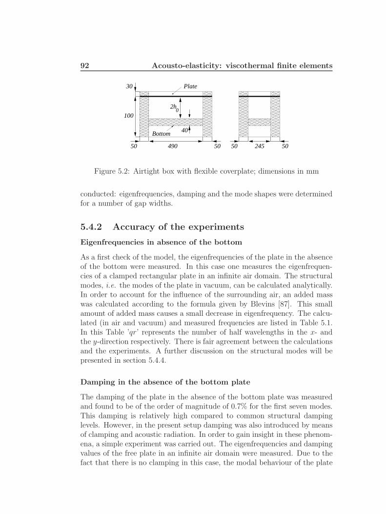
92 Acousto-elasticity: viscothermal finite elements
40
490
100
30
02h
50 50 50 245 50
Bottom
Plate
Figure 5.2: Airtight box with flexible coverplate; dimensions in mm
conducted: eigenfrequencies, damping and the mode shapes were determinedfor a number of gap widths.
5.4.2 Accuracy of the experiments
Eigenfrequencies in absence of the bottom
As a first check of the model, the eigenfrequencies of the plate in the absenceof the bottom were measured. In this case one measures the eigenfrequen-cies of a clamped rectangular plate in an infinite air domain. The structuralmodes, i.e. the modes of the plate in vacuum, can be calculated analytically.In order to account for the influence of the surrounding air, an added masswas calculated according to the formula given by Blevins [87]. This smallamount of added mass causes a small decrease in eigenfrequency. The calcu-lated (in air and vacuum) and measured frequencies are listed in Table 5.1.In this Table ’qr’ represents the number of half wavelengths in the x- andthe y-direction respectively. There is fair agreement between the calculationsand the experiments. A further discussion on the structural modes will bepresented in section 5.4.4.
Damping in the absence of the bottom plate
The damping of the plate in the absence of the bottom plate was measuredand found to be of the order of magnitude of 0.7% for the first seven modes.This damping is relatively high compared to common structural dampinglevels. However, in the present setup damping was also introduced by meansof clamping and acoustic radiation. In order to gain insight in these phenom-ena, a simple experiment was carried out. The eigenfrequencies and dampingvalues of the free plate in an infinite air domain were measured. Due to thefact that there is no clamping in this case, the modal behaviour of the plate

5.4 Experimental validation 93
Mode Eigenfrequency (Hz)qr Measurements Analytical Analytical
(air) (vacuum)
11 96.2 95.9 100.621 130.1 130.4 130.431 181.8 182.6 183.412 247.4 261.7 261.741 253.8 259.7 259.722 280.8 291.2 291.232 322.6 341.0 341.0
Table 5.1: Eigenfrequencies of clamped plate in air
will change. However, an impression of the order of magnitude of the ra-diation damping at least can be obtained. The experimentally determinedfrequencies showed good agreement with finite element results. The dampingfor the first seven modes varied between 0.2 and 0.7%. The clamping of theplate does seem to have only a small influence. If one assumes that the radia-tion damping is relatively low, which was comfirmed by several calculations,the measured damping can be attributed to structural damping. Comparedto the viscothermal damping levels that were measured for low gap widths,however, the structural damping and the damping due to acoustic radiationcan be neglected.
Boundary conditions
Attention was paid to the clamping conditions of the plate. The experimentalresults in Table 5.1 showed fair agreement with the calculations. In theexperiments the bolts were securely fastened. In order to determine theinfluence of the torque, measurements were carried out for small variationsin the torque. No variations in frequencies were observed due to a change inapplied torque.
Linearity
In the experiments the plate was excited with a constant force. In order tocheck whether the system was behaving in a linear way, experiments werecarried out with different excitation levels. The eigenfrequencies and the

94 Acousto-elasticity: viscothermal finite elements
damping values were not affected by the amplitude of excitation. This justi-fies the use of linear theory.
Motion of the bottom plate
In the calculations it was assumed that the box and the bottom plate wererigid and fixed. Since the gap width is a very important parameter in themodel, the motion of the bottom plate was measured with accelerometers fora number of gap widths. In all cases the amplitude of the bottom plate wasvery low, i.e. less than 3% of the amplitude of the flexible coverplate. Thebottom plate was therefore regarded as rigid and fixed.
Variation of the gap width
In the experiments the gap width was varied from 1 to 50 mm. Due tothe fact that the thick bottom plate was not able to tilt inside the box, thein-plane variation in the gap width was small.
5.4.3 Acoustic modes
The acoustic modes are the modes of the air layer when the plate is assumedrigid and fixed (zero velocity). The acoustic modes are calculated from thelow reduced frequency model by omitting the squeeze term:
∂2p
∂x2+∂2p
∂y2− ω2Γ2
c20
p = 0 (5.24)
The edges of the air layer are closed. The corresponding boundary conditionis that the particle velocity is zero. The low reduced frequency model givesthe following boundary condition in terms of the pressure:
∂p
∂n= 0 for x = ±lx and y = ±ly (5.25)
where n is the outward normal. Straightforward separation of variables givesan equation for the acoustic eigenfrequencies:
ω =iπc0
2Γ
√√√√( qlx
)2
+
(r
ly
)2
q = 0, 1, 2 · · · r = 0, 1, 2 · · · (5.26)
Since the propagation constant Γ is a function of the shear wave number theright hand side of (5.26) depends on the frequency and the gap width. Thecomplex eigenfrequencies can now be solved from this equation by a simple

5.4 Experimental validation 95
iterative solving procedure. As starting values, the eigenfrequencies for theinviscid, adiabatic case were used: Γ = i. In Table 5.2 the analytical resultsand the results from finite element calculations are listed for a gap width of1 mm. The calculations were carried out with 20 x 20 linear viscous acousticfinite elements. The table shows good agreement between the analyticalresults and the finite element results. The eigenfrequency of the first acousticmode without viscous or thermal effects is 347 Hz. For low shear wavenumbers the viscous and thermal effects therefore have a significant influenceon the propagation of waves in the air layer.
Mode Eigenfrequency (Hz)qr Analytical Finite elements
10 317.1+32.3i 317.4+32.4i01 651.4+44.8i 652.1+44.8i20 651.4+44.8i 654.1+45.0i11 730.9+47.2i 731.6+47.3i
Table 5.2: Eigenfrequencies of acoustic modes (2h0 = 1 mm)
5.4.4 Structural modes
The eigenfrequencies of the plate in vacuum were calculated with a meshof 20 x 20 linear plate elements and compared with analytical results. Theresults are listed in Table 5.3. The Table shows fair agreement between thenumerical and the analytical results. For the higher modes the results show asmall deviation due to the number of elements. The first seven mode shapesfor the plate in vacuum are given in Figure 5.3. They serve as a referencewhen the mode shapes change as a function of the gap width.
5.4.5 Acousto-elastic modes
In the case of a thin plate backed by a cavity with air, the acousto-elasticcoupling can be very strong. In this section this phenomenon will be demon-strated. For this purpose the first seven eigenfrequencies of the plate will becalculated as a function of the gap width. The eigenfrequencies, dampingvalues and mode shapes are traced in the calculations for gap widths from300 downto 1 mm. For gaps below 50 mm a comparison is made with theexperimental results.
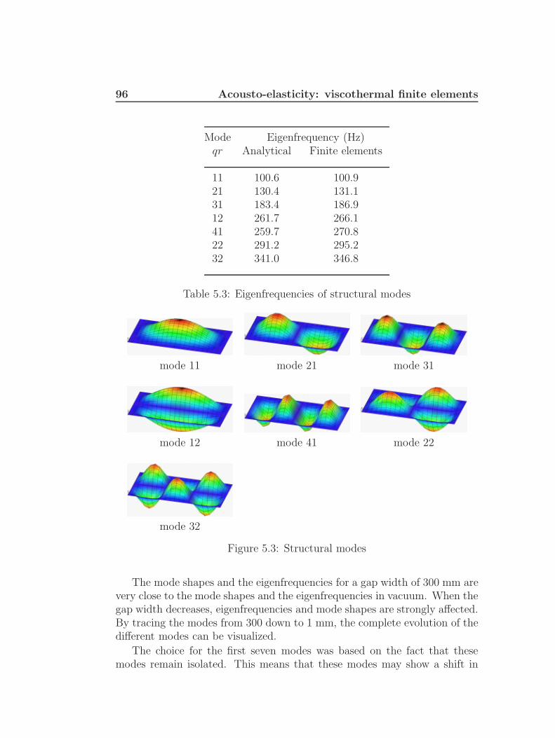
96 Acousto-elasticity: viscothermal finite elements
Mode Eigenfrequency (Hz)qr Analytical Finite elements
11 100.6 100.921 130.4 131.131 183.4 186.912 261.7 266.141 259.7 270.822 291.2 295.232 341.0 346.8
Table 5.3: Eigenfrequencies of structural modes
mode 11 mode 21 mode 31
mode 12 mode 41 mode 22
mode 32
Figure 5.3: Structural modes
The mode shapes and the eigenfrequencies for a gap width of 300 mm arevery close to the mode shapes and the eigenfrequencies in vacuum. When thegap width decreases, eigenfrequencies and mode shapes are strongly affected.By tracing the modes from 300 down to 1 mm, the complete evolution of thedifferent modes can be visualized.
The choice for the first seven modes was based on the fact that thesemodes remain isolated. This means that these modes may show a shift in

5.4 Experimental validation 97
frequency or even mutual cross-overs, but they remain isolated from thehigher (i.e. 8th and higher) modes. The first acoustic eigenfrequency in theabsence of viscous or thermal effects is 347 Hz (see section 5.4.3). Due to theviscous effects this frequency will decrease with decreasing gap width, butthe structural frequencies are always lower. Hence, the first seven modes ofinterest are all structurally dominated modes.
In order to trace the modes from 300 down to 1 mm two types of calcu-lations were carried out. The first type of calculation used standard acousticfinite elements without viscous or thermal effects. These elements were usedfor the calculations for gap widths between 50 and 300 mm. For these gapwidths the shear wave number is very large in the frequency range of interest,so viscous and thermal effects can be neglected. Furthermore the assumptionof constant pressure across the gap width breaks down for high reduced fre-quencies. Note that the damping for these elements is always zero. A meshconsisting of 20 x 20 plate elements, 20 x 20 linear interface elements and 20x 20 x 6 acoustic finite elements was used.
The second type of calculation was based on the use of viscous acousticfinite elements. These elements were used for gap widths below 50 mm. Amesh consisting of 20 x 20 linear plate elements, 20 x 20 linear interfaceelements and 20 x 20 linear viscothermal acoustic finite elements was used toperform these calculations. As a check on the accuracy of the finite elementmodel for the experimental setup, the uncoupled modes for the plate andthe air layer were calculated and compared to analytical solutions in sections5.4.3 and 5.4.5 respectively.
The influence of the air on the upper side of the plate is not taken intoaccount in the calculations. In section 5.4.2 it was demonstrated that theair on the upper side of the panel causes a slight decrease in eigenfrequency.For low gap widths however this effect can be neglected compared to theshift in frequency due to the pressure in the layer. The air on the upperside introduces an energy loss due to radiation damping. However, in section5.4.2 it was shown that the radiation damping and the structural dampingare very low compared to the viscothermal damping for small gap widths.
Eigenfrequency
In Figure 5.4 the eigenfrequency is depicted versus the gap width 1. Thelabels for the different modes are based on the original modes in vacuum (seeTable 5.3). The experimental results and the finite element results show fairagreement. For the lower modes the results are very good. For the higher
1The eigenvalue calculation results in complex valued angular frequencies: ω = ωr+iωi.For viscous damping the undamped natural frequency is then calculated from: ωn = |ω|

98 Acousto-elasticity: viscothermal finite elements
modes the finite element results start to be less accurate. This can mainlybe attributed to the behaviour of the plate elements, as can be seen in theresults for the structural modes. But in general the agreement is satisfyingfor all modes under consideration. At a gap width of 50 mm the transitionfrom the results with standard acoustic elements to the results with viscousfinite elements is good. There seems to be a slight bend in the curve, but thedifference in frequency between both calculations is less than 0.7% for thisgap width.
The Figure shows a very large shift in eigenfrequency for the differentmodes. The coupled eigenfrequencies differ considerably from the uncoupledstructural eigenfrequencies. This means that in the case of narrow gaps it isessential to take into account the acousto-elastic coupling. Different kinds ofbehaviour can be observed. The second mode, for instance, shows a steadydecrease with decreasing gap width. The first mode however first increasesand then decreases with decreasing gap width. At a gap width of about 100mm the eigenfrequencies cross. In order to analyse this in more detail, severalcalculations were carried out in this region. The results clearly indicate thatthere is indeed a cross-over. The 31 mode also exhibits cross-over behaviourwith other modes. This was confirmed by the measurements.
Damping
In Figure 5.5 the dimensionless damping coefficient is depicted versus thegap width for the first and second modes 2. For small gaps the dampingincreases by up to 25%. This high level of damping can be attributed to theviscous effects in the air layer. The second mode is an asymmetric mode thatinduces a strong pumping of air in the layer. The corresponding high rate ofshear results in significant viscous losses. Thermal effects have a very smallinfluence on the damping, as was already demonstrated by Fox and Whitton[67]. The structural damping and the damping due to acoustic radiation arelow compared to the viscothermal damping mechanisms for small gap widths.The Figure shows fair agreement between calculations and experiments. Thisindicates that the energy dissipation in the layer is correctly described withthe new finite element model.
The present investigation allows a detailed comparison between theoryand experiments. Because of the systematic approach that was used to de-velop and validate the models, the different aspects can be addressed in detail.The specially developed experiments offer a good insight in the phenomena
2The eigenvalue calculation results in complex valued angular frequencies: ω = ωr+iωi.For viscous damping the dimensionless damping coefficient is then calculated from: ξ =ωi|ω| × 100 %

5.4 Experimental validation 99
and allow a qualitative and quantitative comparison with calculations. Inthe present test case with the closed box and a thin flexible plate the fre-quency shifts were substantial. Furthermore, the damping values were veryhigh. The agreement between theory and experiment is good, even on alinear scale.
Mode shapes
The mode shapes were calculated and measured for a number of gap widths.In Figure 5.6 the calculated mode shapes are depicted for gap widths of300, 50 and 10 mm. The labels of the modes in this Figure are based onthe corresponding mode shapes in vacuum. The modes shapes are almostreal; the phase differences between the displacements measured on differentlocations of the plate are very small. The Figures indicate that the shapeof the asymmetric modes is not affected by the gap width. The symmetricmodes however show a dramatic change in shape. For small gaps, the 11mode starts to resemble the 31 mode. A physical interpretation for thesephenomena will be given in the next section.
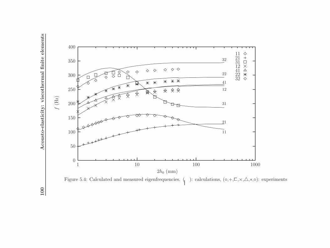
100
Aco
ust
o-e
last
icit
y:
vis
coth
erm
al
finit
eele
ments
32224112312111
32
22
41
12
31
21
11
2h0 (mm)
f(H
z)
1000100101
400
350
300
250
200
150
100
50
0
Figure 5.4: Calculated and measured eigenfrequencies. ( ): calculations, (,+,2,×,4,∗,): experiments

5.4 Experimental validation 101
2111
11
21
2h0 (mm)
ξ(%
)
1086420
25
20
15
10
5
0
Figure 5.5: Dimensionless damping coefficient versus gap width. ( ): cal-culations, (,+): experiments
5.4.6 Physical interpretation
The shifts in eigenfrequency and the changes in mode shape can be explainedin terms of (generalized) added mass and (generalized) added stiffness.
Added mass
Due to the squeeze motion of the plate the air is put into motion. This motionof the air is experienced by the plate as an added mass. For the closed cavity,the motion of the air is related to the pumping mechanism. For asymmetricmodes, the air is pumped back and forth very efficiently. This pumping effectincreases as the gap width decreases. Therefore the added mass increases andthe frequency decreases with decreasing gap width.
Added stiffness
The increase in frequency that was observed for some modes can be attributedto an added stiffness effect. For the symmetric modes, the deformation ofthe coverplate is accompanied by a significant change in cavity volume (seeFigure 5.7). This change in volume causes a pressure disturbance in thecavity. In the frequency range of interest, the acoustic wavelength is largecompared to the cavity dimensions. Since the pressure disturbance is inphase with the motion of the plate, the plate experiences an added stiffnesseffect. As the pressure disturbance increases with decreasing gap width, the

102 Acousto-elasticity: viscothermal finite elements
Mode h0 = 10 mm h0 = 50 mm h0 = 300 mm
11
21
31
12
41
22
32
Figure 5.6: Acousto-elastic modes shapes
eigenfrequency will increase. Asymmetric modes do not induce a change incavity volume: they do not experience an added stiffness effect. Due to thestiffness effect the shape of the symmetric modes also changes. The generaltrend is that mode shapes tend to a shape for narrow gaps for which the netvolume change is zero (see Figure 5.6). This means that the added stiffnesseffect will vanish, and the added mass effect takes over (see Figure 5.4). Thisexplains the shape of the curves of the eigenfrequencies versus the gap width.

5.4 Experimental validation 103
p p
pV
+V-V
p +p
0 0
0
000
+V
V
Figure 5.7: Change in cavity volume for the first and the second mode
5.4.7 Dimensionless parameters
The dimensionless parameters are a function of the geometry, the materialproperties and the frequency. In the experimental setup the gap width isvaried from 50 down to 1 mm, while the frequency varies between 50 and350 Hz.
The ratio between the inertial forces and the viscous forces is given bythe shear wave number. For the experimental setup, the shear wave numbervaries from 4.5 to 600. This means that for small gap widths and low frequen-cies the effects of viscosity have to be taken into account. In the frequencyrange of interest, the effects of viscosity are very small for gap widths largerthan 50 mm. The use of standard acoustic elements is therefore justified forthese larger gap widths.
For low values of the shear wave number, as σ is a constant for air, thethermal conductivity can play an important role. For the experimental setupthese thermal effects are relatively small. However, one has to be careful notto generalize this statement. For very small gap widths or other materialsfor instance the effects can be very significant. Then the process in the layerhas to be regarded as isothermal, rather than isentropic.
In the low reduced frequency theory the acoustic wavelength must belarge compared to both the gap width and the boundary layer thickness. Forthe experimental setup and gap widths smaller than 50 mm: k < 0.3 andk/s < 10−3. This means that the use of the low reduced frequency model isjustified for small gap widths.

104 Acousto-elasticity: viscothermal finite elements
5.5 Conclusions
Based on the research presented in this chapter, the following conclusionscan be drawn:
• new viscothermal finite elements were developed, based on the lowreduced frequency model. Layer elements and tube elements were im-plemented in the finite element package B2000;
• viscothermal elements with different cross sections or layer thicknessescan be coupled. The viscothermal elements can also be coupled tostandard acoustic finite elements;
• the viscothermal layer elements can be coupled to structural elementswith the standard interface elements. The new acousto-elastic finite el-ement model can be used to calculate the response of complex systems;
• convergence tests confirm that the elements function properly;
• eigenfrequency calculations for the frequency-dependent acousto-elasticsystem can be performed using an iterative approach;
• frequency response calculations can be performed efficiently with astraightforward component mode technique, using the structural modesand the acoustic modes for the inviscid, adiabatic case;
• experimental verification shows that the acousto-elastic interaction be-tween a viscothermal air layer and a vibrating flexible plate is correctlydescribed by the finite element model. The behaviour of the systemis strongly affected by the presence of the air layer. Eigenfrequencies,damping values and mode shapes change as a function of the layer thick-ness. It is therefore important to include the acousto-elastic coupling;
• a significant amount of energy can be dissipated in the layer by meansof viscous shear. This may result in substantial damping values for anadjacent structure. The amount of damping is related to the pump-ing effect in the layer and thus on the coupled vibration mode of thestructure.

Chapter 6
Engineering applications
6.1 Solar panels during launch
During the launch of a spacecraft the solar panels are stowed alongside thestructure (see Figure 6.1) 1.
Yoke panel
Panel 2
Hold-down stackHinge
Panel 1
Satellite sidewall
Figure 6.1: SOHO wing in stowed position, side view
The panels are connected by hinges and held together by spacers andhold-down brackets. In space, the array is deployed by cutting kevlar cableswith a thermal knife. Springs inside the joints will then open the wing. Thesolar panels are relatively large, light and stiff. In Figure 6.2 a sketch ispresented of a deployed solar array.
During the launch phase the spacecraft and the panels are exposed tosevere vibrations. Any damage to the wing or the satellite can lead to crit-ical failures. A structural failure may jeopardize the satellite mission. Itis therefore important to have a good understanding of the behaviour andthe characteristics of the folded pack of solar panels. Before a spacecraft islaunched, several qualification tests are carried out to ensure that the panels
1SOHO= SOlar and Heliospheric Observatory

106 Engineering applications
0.392 1.415
1.5
Yokepanel
Panel 1 Panel 2sidewall
0.3070.307
1.29
4
2.3Satellite
Figure 6.2: Deployed SOHO wing, top view, dimensions in m
can withstand the expected load. For this purpose, the stack of panels isattached to a vibration Table (see Figure 6.3).
Excitation axis
Figure 6.3: Test setup for z-axis excitation
Tests are usually carried out for out-of-plane (z-direction) and in-plane (xand y-directions) excitation. In the frequency range of interest, e.g. 5-100 Hz,a sine sweep vibration is performed. Eigenfrequencies, damping coefficientsand acceleration, strain and force levels are measured. In addition, randomvibration tests are carried out.
The vibration tests indicate that the thin layers of air that are trapped
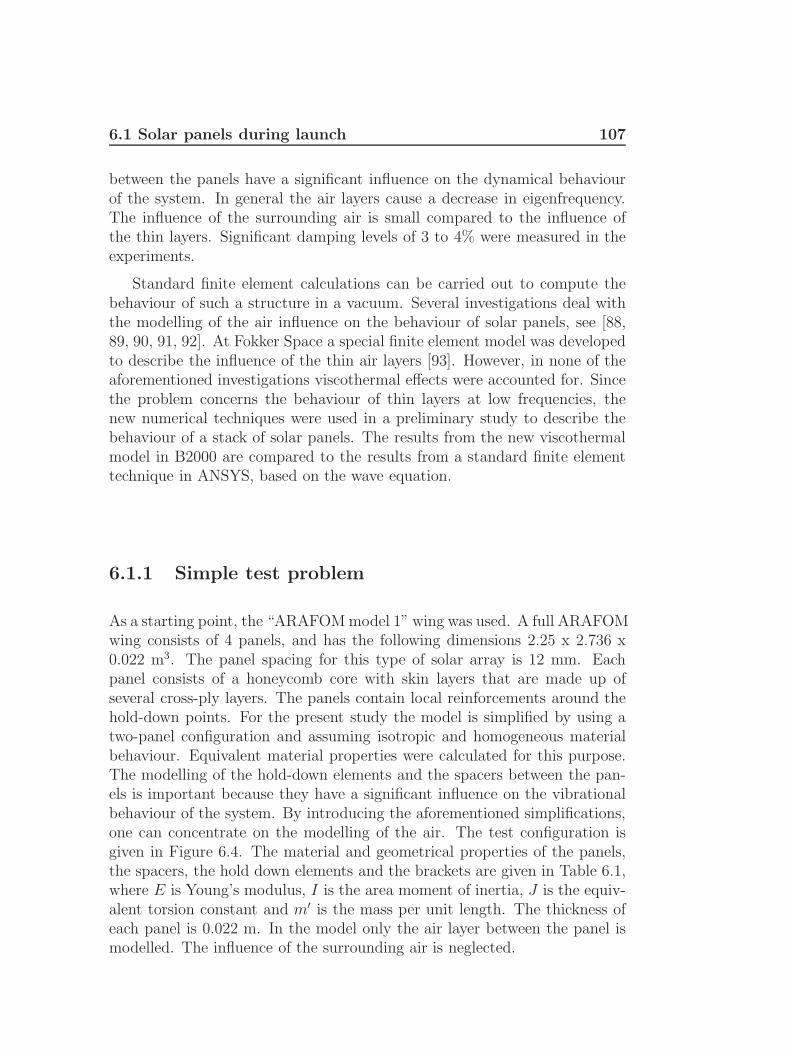
6.1 Solar panels during launch 107
between the panels have a significant influence on the dynamical behaviourof the system. In general the air layers cause a decrease in eigenfrequency.The influence of the surrounding air is small compared to the influence ofthe thin layers. Significant damping levels of 3 to 4% were measured in theexperiments.
Standard finite element calculations can be carried out to compute thebehaviour of such a structure in a vacuum. Several investigations deal withthe modelling of the air influence on the behaviour of solar panels, see [88,89, 90, 91, 92]. At Fokker Space a special finite element model was developedto describe the influence of the thin air layers [93]. However, in none of theaforementioned investigations viscothermal effects were accounted for. Sincethe problem concerns the behaviour of thin layers at low frequencies, thenew numerical techniques were used in a preliminary study to describe thebehaviour of a stack of solar panels. The results from the new viscothermalmodel in B2000 are compared to the results from a standard finite elementtechnique in ANSYS, based on the wave equation.
6.1.1 Simple test problem
As a starting point, the “ARAFOM model 1” wing was used. A full ARAFOMwing consists of 4 panels, and has the following dimensions 2.25 x 2.736 x0.022 m3. The panel spacing for this type of solar array is 12 mm. Eachpanel consists of a honeycomb core with skin layers that are made up ofseveral cross-ply layers. The panels contain local reinforcements around thehold-down points. For the present study the model is simplified by using atwo-panel configuration and assuming isotropic and homogeneous materialbehaviour. Equivalent material properties were calculated for this purpose.The modelling of the hold-down elements and the spacers between the pan-els is important because they have a significant influence on the vibrationalbehaviour of the system. By introducing the aforementioned simplifications,one can concentrate on the modelling of the air. The test configuration isgiven in Figure 6.4. The material and geometrical properties of the panels,the spacers, the hold down elements and the brackets are given in Table 6.1,where E is Young’s modulus, I is the area moment of inertia, J is the equiv-alent torsion constant and m′ is the mass per unit length. The thickness ofeach panel is 0.022 m. In the model only the air layer between the panel ismodelled. The influence of the surrounding air is neglected.

108 Engineering applications
2.1
1.2
0.6
2.25
1.05
0.75
2.7
Air layer
element
Bracket
Spacer
Hold-down
0.012
0.017
0.063
Figure 6.4: ARAFOM model problem, top view (left), front view (right),dimensions in m, panel thickness is 0.022 m
E (Pa) I (m4) J (m4) A (m2) m′ (kg/m)
solar panel 52.90 · 1012 −− −− −− −−spacer 108 · 109 0.87 · 10−9 3.50 · 10−6 1.0 · 10−4 7.283
hold-down 108 · 109 2.50 · 10−9 10.0 · 10−6 1.0 · 10−4 2.544bracket 70 · 109 39.0 · 10−9 0.12 · 10−6 1.0 · 10−4 5.088
Table 6.1: Material and geometrical data test configuration
6.1.2 Finite element calculations
The panels were modelled using 18 x 15 plate elements. In B2000 the ro-tation around the z-axis was suppressed for these elements. Each spacerwas modelled with a line of 6 beam elements, each hold-down structure wasmodelled with a line of 6 beam elements and each bracket was also mod-elled with a line of 6 beam elements. The lower ends of the brackets werefully clamped. The beam elements in the finite element models account forbending, extension and torsion. The air was modelled in different ways. InANSYS, the air was modelled using 3-dimensional acoustic volume elements.These elements are based on the standard wave equation and therefore donot include viscothermal effects. Compressibility however is accounted for.Incompressible behaviour in ANSYS can be artificially simulated by takingthe speed of sound to be very large. Three elements were used across thelayer thickness. The air model in B2000 was based on the low reduced fre-quency model. The new viscothermal elements were used to calculate the

6.1 Solar panels during launch 109
pressure distribution in the layer. At the edges of the air layer a pressurerelease condition (p = 0) was imposed. Thus, the influence of the surround-ing air is neglected. Calculations indicate that this is justified, both froma frequency and a damping point of view. An overview of element types isgiven in Table 6.2.
In ANSYS and B2000 the air elements were coupled to the structuralelements. In ANSYS a key option has to be activated for acoustic elementsnot adjacent to the structure. In B2000 interface elements were used toestablish the coupling.
ANSYS B2000
panels SHELL63 Q4.STspacer BEAM3 B2hold-down BEAM3 B2bracket BEAM3 B2air FLUID30 Q4.VISC
Table 6.2: Element types for the finite element models
6.1.3 Results for vacuum
The eigenfrequencies for the structure in vacuum are listed in Table 6.3. Themodes can be classified as in-phase and out-of-phase modes (see Figure 6.5).Mode 5 is a local mode.
Out-of-phase In-phase
Figure 6.5: Out-of-phase modes and in-phase modes
In the fifth column of Table 6.3 the displacement ratio, calculated usingANSYS, is given. The displacement ratio is defined as the ratio between themaximum deflection of the lower panel and the maximum deflection of the

110 Engineering applications
upper panel. A ratio larger than 1 means that the lower panel is relativelyactive, while for a ratio smaller than 1 the lower panel is relatively inactive.
Mode Type Frequencies (Hz) RatioANSYS B2000 ANSYS
1 Out 44.14 44.65 0.512 In 47.89 48.62 1.963 In 48.64 49.38 0.474 Out 49.53 50.11 0.125 Local 51.01 51.67 2.866 Out 51.37 52.14 1.897 Out 51.88 52.61 0.568 In 53.21 54.05 2.709 Out 53.95 54.53 0.3910 In 55.20 55.86 2.6311 Out 60.67 61.27 0.3112 Out 60.69 61.31 0.4013 In 62.08 62.77 2.7014 In 63.31 64.07 3.03
Table 6.3: Eigenfrequencies ARAFOM test problem in vacuum
The results of the two finite element models show good agreement. Thisis a requirement for making any judgements about the influence of the airlater in the investigation. The small differences are caused by the differenttype of plate elements.
6.1.4 Results for air
The eigenfrequencies of the system in air are listed in Table 6.4. The re-sults from calculations with ANSYS and B2000 are given. Again, the modescan be classified as in-phase and out-of-phase modes. The results of B2000calculations with and without viscothermal effect are given in Table 6.5 2.
Table 6.4 shows that the order of the modes has changed. The lowermodes are now all low frequency out-of-phase modes. This is not surprising,
2The eigenvalue calculation results in complex valued frequencies: ω = ωr + iωi. Forviscous damping the natural frequency is then calculated from: ωn = |ω|. The dimension-less damping coefficient is: ξ = ωi
|ω| × 100%

6.1 Solar panels during launch 111
Mode Type Frequencies (Hz) RatioANSYS B2000 ANSYS
Compr Incompr Inviscid ComprAdiabatic
1 Out 21.13 21.27 21.55 0.922 Out 23.84 24.13 24.80 0.933 Out 23.98 24.25 24.60 0.914 Out 25.74 25.95 26.50 0.925 Out 29.81 30.10 30.46 0.916 Out 30.94 31.10 31.60 0.957 Out 33.06 33.29 33.55 0.948 Out 34.21 34.37 34.69 0.959 In 47.48 47.49 48.26 1.1010 Out 48.28 48.88 49.17 1.0411 In 48.87 49.16 49.70 0.9712 In 50.41 50.44 51.14 0.9313 In 52.93 52.93 53.85 1.0514 In 54.92 54.92 55.66 1.02
Table 6.4: Eigenfrequencies ARAFOM test problem in air
since out-of-phase vibrations introduce a significant pumping effect. For thelayer with open ends, the added stiffness is very small. Consequently, thelarge amount of added mass for the out-of-phase modes causes a drasticdecrease in frequency. In practical situations, however, the importance ofthese modes is limited. In the vibration tests for the SOHO configuration forinstance, described in section 6.1, these modes were not detected in the sinevibration test because they were not excited by the base excitation.
Secondly, the Table shows that the in-phase modes are affected little bythe presence of the air layer. For the in-phase modes there is no strongpumping effect. The pumping for in-phase modes originates from the factthat the panels vibrate with different amplitudes. These effects however arerelatively small. Table 6.4 shows that the displacement ratio between thepanels is almost equal to 1 for all modes. It is interesting to analyse thevalues of the displacement ratio in vacuum. Table 6.3 shows that the ratioin vacuum varies between 0.3 and 3. Thus, in vacuum the deflections ofboth panels can be quite different. This indicates that the air layer providescoupling between the two panels, and forces them to vibrate with the same

112 Engineering applications
Mode Type Frequencies (Hz) Damping (%)B2000 B2000 B2000
inviscid full fulladiabatic
1 Out 21.55 21.22 1.682 Out 24.80 24.40 1.743 Out 24.60 24.40 1.734 Out 26.50 26.13 1.505 Out 30.46 30.09 1.326 Out 31.60 31.25 1.187 Out 33.55 33.18 1.178 Out 34.69 34.33 1.109 In 48.26 48.31 0.0910 Out 49.17 48.69 0.9911 In 49.70 48.73 0.8712 In 51.14 51.13 0.0213 In 53.85 53.85 0.0014 In 55.66 55.66 0.00
Table 6.5: Influence of viscothermal effects
amplitude. Hence, the pumping effects for these modes is small. Theseconsiderations are very helpful when analysing the results of the differentmodels. The validity of the various assumptions for the test problem underconsideration will now be discussed.
Compressibility
The influence of the compressibility can be analysed by simply comparingthe ANSYS results for compressible and incompressible behaviour in Table6.4. The values indicate that the compressibility effects are very small, es-pecially for the in-phase modes. A parameter that can be used to estimatethe influence of compressibility is the ratio between the plate dimensions andthe acoustic wavelength. For the present test case, the acoustic wavelength istypically large compared to the plate dimensions while the ends of the layerare open. Compressibility effects are therefore small.

6.1 Solar panels during launch 113
Constant pressure across the gap width
The influence of the assumption of constant pressure across the gap widthcan be analysed by comparing the ANSYS results for compressible behaviourand the B2000 results for inviscid, adiabatic behaviour in Table 6.4. InANSYS three linear elements were used across the gap width. Regardingthe deviations in the vacuum frequencies, there is no significant differencebetween the two results. This indicates that the assumption of constantpressure is reasonable.
Viscothermal effects
The influence of viscothermal effects can be deduced from Table 6.5. Theshear wave number for the present configuration varies between 15 and 25,which indicates that viscothermal effects could be important. The frequenciesof all the modes are affected very little by the viscothermal effects, especiallyfor the in-phase modes. The in-phase modes do not introduce large velocitiesand pressures in the air and thus the air effects remain small for these modes.There is a significant amount of damping for the out-of-phase modes. Thesemodes introduce a strong pumping of the air, resulting in significant viscouslosses. However, these modes are very difficult to excite in the tests.
It can be concluded that viscothermal effects have very little influencein the present test case. The frequencies are not affected and the dampinglevels for the important in-phase modes remain low.

114 Engineering applications
6.1.5 Practical considerations
In the previous section, it was demonstrated that the introduction of severalassumptions is justified for the test problem. Compressibility and viscother-mal effects are small, and the pressure can be assumed to be constant acrossthe gap width.
The damping levels that were found in the sine vibration tests cannot beexplained by these calculations. There are probably other important effectsin the SOHO tests that were not accounted for in the current finite elementmodels. In the tests, for instance, cables are present between the panels.These cables are tied together and obstruct the air flow in the layer. Theinfluence of barriers in the air layer will be investigated in section 6.4. Inthis section it is demonstrated that barriers can have a very large influenceon the energy dissipation in a thin layer.
Finally, the simple test configuration consists of two panels with one airlayer. There are several configurations in use with more than two panels.The behaviour of such systems with multiple air layers is more complicated.

6.2 Inkjet print head 115
6.2 Inkjet print head
The newly developed techniques were used in the design of inkjet print heads.In cooperation with Oce Technologies B.V. projects were defined in order todevelop a theoretical model for the description of the dynamical behaviourof a print head. This section briefly discusses the techniques that were usedand gives an impression of the results that were obtained. Some literature isavailable on inkjet print heads, see e.g. [94, 95, 96, 97], mostly dealing withthe propagation of waves in a single flexible channel using analytical models.
Epoxy
Channel plate
Piezo
Nozzle
Reservoir
Channel
Figure 6.6: Inkjet print head
An inkjet print head consists of a channel plate with a large number ofparallel ink channels (see Figure 6.6). A nozzle is attached to one side ofthe channel. The other side of the channel is connected to the ink reservoir.Piezo-elements on top of the channels are used for activation. A pressure dis-turbance in the channel is created by means of electric piezo-activation. Thepiezo expands and consequently a pressure disturbance is introduced. Pres-sure waves start travelling into the channel and the nozzle. By deactivatingthe piezo at the right moment, the pressure can increase to a level at whicha drop will be released from the nozzle. Clearly, the aim of the print head isto deliver a drop of ink of the right size at the right time at the right place.
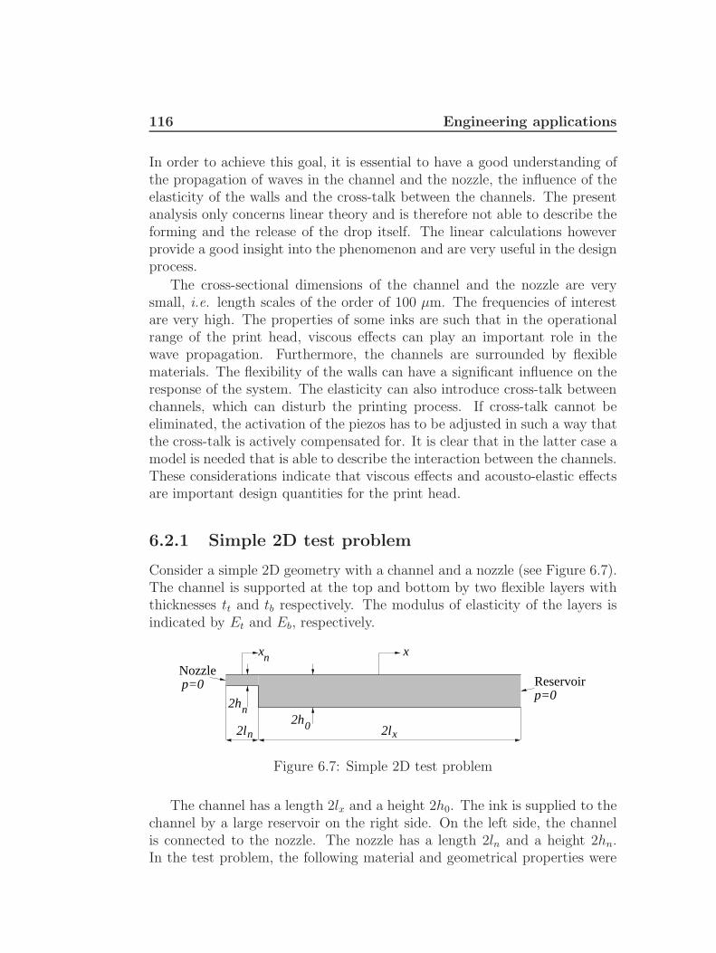
116 Engineering applications
In order to achieve this goal, it is essential to have a good understanding ofthe propagation of waves in the channel and the nozzle, the influence of theelasticity of the walls and the cross-talk between the channels. The presentanalysis only concerns linear theory and is therefore not able to describe theforming and the release of the drop itself. The linear calculations howeverprovide a good insight into the phenomenon and are very useful in the designprocess.
The cross-sectional dimensions of the channel and the nozzle are verysmall, i.e. length scales of the order of 100 µm. The frequencies of interestare very high. The properties of some inks are such that in the operationalrange of the print head, viscous effects can play an important role in thewave propagation. Furthermore, the channels are surrounded by flexiblematerials. The flexibility of the walls can have a significant influence on theresponse of the system. The elasticity can also introduce cross-talk betweenchannels, which can disturb the printing process. If cross-talk cannot beeliminated, the activation of the piezos has to be adjusted in such a way thatthe cross-talk is actively compensated for. It is clear that in the latter case amodel is needed that is able to describe the interaction between the channels.These considerations indicate that viscous effects and acousto-elastic effectsare important design quantities for the print head.
6.2.1 Simple 2D test problem
Consider a simple 2D geometry with a channel and a nozzle (see Figure 6.7).The channel is supported at the top and bottom by two flexible layers withthicknesses tt and tb respectively. The modulus of elasticity of the layers isindicated by Et and Eb, respectively.
Nozzlep=0
2ln
p=0Reservoir
n
2lx
x
n
x
2h0
2h
Figure 6.7: Simple 2D test problem
The channel has a length 2lx and a height 2h0. The ink is supplied to thechannel by a large reservoir on the right side. On the left side, the channelis connected to the nozzle. The nozzle has a length 2ln and a height 2hn.In the test problem, the following material and geometrical properties were

6.2 Inkjet print head 117
used:
ρ0 = 1200 kg/m3 ; µ = 15 · 10−3 Ns/m2
c0 = 1200 m/s ; (6.1)
Et = 70 · 109 N/m2 ; Eb = 70 · 109 N/m2
tt = 1 · 10−3 m ; tb = 0.25 · 10−3 m
lx = 3.5 · 10−3 m ; ln = 100 · 10−6 m
h0 = 100 · 10−6 m ; hn = 17 · 10−6 m
The ratio of specific heats γ is set equal to 1, so that the polytropic constantn(sσ) automatically takes the value of 1. At the nozzle exit and the reser-voir side of the channel the pressure perturbation is set equal to zero. Theexcitation is introduced by means of a piezo-electric material on top of thechannel. The steady state and the transient response of the system due tothis excitation will now be described by a number of simple models. The ve-locity at the centre of the nozzle exit is calculated, because this is a quantitythat can also be determined experimentally (see section 6.2.2). With thissimple 2D model the effects of viscosity, wall elasticity, and the use of finiteelements are illustrated. These techniques are then used in section 6.2.2 forthe design of a new print head.
Model with rigid walls
0h he
p=0p=0
ωi t
Figure 6.8: Model with rigid walls
In the model with rigid walls the walls of the nozzle and the nozzle are allrigid. The top wall of the channel performs a small normal oscillation withamplitude h0h. The other walls are fixed. The differential equations for thissituation are (see chapter 2 and Appendix B):
channel :∂2p
∂x2− Γ2p =
1
2n (sσ) Γ2h
nozzle :∂2p
∂x2− Γ2
np = 0 (6.2)

118 Engineering applications
where the subscript n refers to the nozzle. The boundary conditions at theexit of the nozzle and the reservoir side of the channel are p = 0. By assumingmass conservation and continuity of pressure on the interface between thenozzle and the channel, the problem can be solved. Once the presssuredistribution is known, the dimensionless velocity at the centre of the nozzlecan be calculated from (see chapter 2 and Appendix B for a layer geometry):
vxn = − iγ
1
cosh(s√i) − 1
∂p∂x
(6.3)
Model with spring walls
h he
k
0
k t
i t
ω
0 th h e i tω
i t
b
ω
p=0
p=0 h h e0 b
Figure 6.9: Model with spring walls
In this 2-dimensional model the top and bottom walls of the nozzle are rigidand fixed. The walls of the channels are supported at the top and bottomby an elastic foundation of massless springs. The stiffness per unit area ofthe springs at the top and the bottom of the channel is:
kt =Ettt
; kb =Ebtb
(6.4)
where Et and Eb represent Young’s modulus for the top and bottom mate-rials and tt and tb represent the thicknesses of the supporting layers. Theupper ends of the top springs perform a harmonic displacement oscillation.The lower ends of the bottom springs are fixed. The differential equationsgoverning the behaviour of this model are:
channel :∂2p
∂x2− Γ2p =
1
2n (sσ) Γ2 [ht − hb]
nozzle :∂2p
∂x2− Γ2
np = 0

6.2 Inkjet print head 119
top springs : ht = h+p
γkt(6.5)
bottom springs : hb = − p
γkb
where the dimensionless stiffnesses are given by:
kt =h0
ρ0c20
kt ; kb =h0
ρ0c20
kb (6.6)
In physical terms, the dimensionless stiffness represents the ratio betweenthe stiffness of the springs and the stiffness of the ink layer. If the ink actslike a one-dimensional spring, the stiffness is equal to ρ0c
20/h0. Combining
the equations leads to the following two equations to be solved:
channel :∂2p
∂x2− Γ2
[1 +
1
2
n(sσ)
γ
(1
kt+
1
kb
)]p =
1
2n(sσ)Γ2h
nozzle :∂2p
∂x2− Γ2
np = 0 (6.7)
Again, by demanding conservation of mass and continuity of pressure, thecoupling between the channel and the nozzle is established. With the bound-ary conditions at the nozzle exit and the reservoir side of the channel thesolution is obtained. The dimensionless velocity can then be calculated.
Expression (6.7) shows that the propagation of waves in the channel isaffected by the flexibility of the walls. If the spring stiffnesses are very largecompared to the fluid stiffness, i.e. kt 1 and kb 1, the model evidentlyreduces to the rigid wall model. The viscothermal and elastic effects can alsobe interpreted in terms of an effective speed of sound:
ceff =c0i
Γ
1√1 + 1
2n(sσ)γ
(1kt
+ 1kb
) (6.8)
This expression shows that the flexibility of the walls reduces the effectivespeed of sound.
Model with finite elements
A schematic drawing of the finite element model is given in Figure 6.10.The nozzle and the channel are modelled with the new viscothermal
Q4.VISC elements. The top and the bottom supporting layers are modelledwith 3-dimensional HE8.S elements. These structural elements are coupledto the viscothermal elements with INT.8 interface elements. Frequency re-sponse calculations were carried out for a prescribed displacement. In the

120 Engineering applications
INT.8
HE8.S
R2
HE8.S
p=0INT.8
Q4.VISC
p=0t t
t b
Figure 6.10: Model with finite elements
current version of B2000 a displacement could not be prescribed. This prob-lem was solved by connecting massless rod elements, type R2, to the topnodes of the structural volume elements. The top ends of the rods werefixed. The rods have a very large stiffness that dominates the structuralcontribution from the HE8.S elements. By imposing the correct force on thelower nodes of the rods, the corresponding displacement could be prescribed.
The velocity at the nozzle exit was extracted from the pressure results,since the pressure is the only degree of freedom for the viscothermal ele-ments. The pressure at the nozzle exit is zero. In the finite element analysislinear elements were used. The velocity at the nozzle exit can therefore beapproximated by:
vxn ∼= −i
γ
1
cosh(s√i) − 1
γω
ρ0c0
nexn
2lnpe+1 (6.9)
where nexn is the number of elements in the nozzle and pe+1 is the pressurein the nodal point just to the right of the nozzle exit.
Frequency response results
The velocity at the nozzle exit is divided by the amplitude of the displacementfor this linear system. The transfer function H (ω) is:
H (ω) =vxn (ω)
h0h (ω)(6.10)
The amplitude of the transfer function is given as a function of the fre-quency in Figure 6.11.
Figure 6.11 shows that for this type of ink the viscosity has a significanteffect on the propagation of waves (compare the results for the rigid inviscid

6.2 Inkjet print head 121
FEM (mass)
springs, FEM (no mass) rigid
rigid inviscid
f (kHz)
|H(ω
)|
10090807060504030
1012
1010
108
106
104
102
Figure 6.11: Frequency response simple 2D test problem
case and the rigid case). For the present test case the shear wave numbervaried between 6 and 11. For these low shear wave numbers the viscosity isvery important. The eigenfrequency of the system is an important param-eter for the print head since it is related to the velocity of the waves andthus determines the most efficient activation strategy of the piezo. Dampingcauses a decay of pressure waves in time. If a drop has been released fromthe nozzle, the pressure must decrease to a low level before the piezo can beactivated again, otherwise the jetting history can affect the printing process.In the last part of this section this will be illustrated with the transient timeresponse of the system.
The flexibility of the walls can affect wave propagation. When the wallsare very flexible, the speed of the waves decreases and the transfer functionis affected. In a realistic print head the flexibility is an aspect of seriousconcern. The finite element calculations with a massless piezo show goodagreement with the results of the spring model.
Figure 6.11 shows that for the present problem the mass of the piezohas a large influence on the amplitude of the transfer function. In this testcase the excitation forces the whole piezo to move up and down. However,the imposed displacement excitation is not very realistic for the print headunder consideration. In reality the piezo is activated electrically and underthe applied voltage it will deform and introduce a pressure disturbance in thechannel. The piezo is embedded in the print head and will not vibrate as a

122 Engineering applications
whole. This is confirmed by measurements. Thus, in practical situations themass of the piezo will not have a large effect on the response of the system.
Transient results
The transient response of the channel can be calculated by means of Fouriertransforms. Suppose the top of the piezo is subjected to a displacementhistory h0h(t). The Fourier transform of the displacement history, h0h (ω),is given by:
h0h (ω) =∫ ∞−∞
h0h (t) e−iωtdt (6.11)
The velocity at the nozzle exit in the frequency domain, vxn (ω), is obtainedby simply multiplying the excitation spectrum with the transfer functionH (ω):
vxn (ω) = H (ω)h0h (ω) (6.12)
The transient response is obtained through the inverse Fourier transform:
vxn (t) =1
2π
∫ ∞−∞
vxn (ω) eiωtdω (6.13)
The transient response was calculated with the analytical rigid wall modeland the analytical model where the walls were represented by springs. Theexcitation signal is:
h0h(t) =
0 : t < 010 · 10−9 : 0 < t < 1 · 10−5
0 : t > 1 · 10−5(6.14)
A fast Fourier algorithm was used to calculate the Fourier transforms. Atime span from -0.2 ms to 0.2 ms was used, with a total of 212 points. Thetime responses of the rigid wall model and the flexible spring model are givenin Figure 6.12.
Due to the activation of the piezo, a pressure disturbance is introducedin the channel. Waves start propagating, reflecting off the open ends at thereservoir side of the channel and the nozzle exit. By deactivating the piezo atthe right moment, the pressure in the channel and the velocity in the nozzlecan increase to a level at which a drop will be released. A good timing inthe activation signal is very important in the printing process. It is evidentthat the speed of the waves, and thus the viscosity of the fluid, are importantfactors.
The Figure shows a decay of the ink velocity at the nozzle exit in time.The decay is caused by the dissipation of energy by means of viscous shear.

6.2 Inkjet print head 123
Pulse signal
t (s)
vxn
(m/s
)
20 · 10−515 · 10−510 · 10−55 · 10−50−5 · 10−5
1
0.8
0.6
0.4
0.2
0
-0.2
-0.4
-0.6
-0.8
-1
Figure 6.12: Transient response rigid wall and spring wall model 2D testproblem rigid walls ( ), spring walls (−−)
The decay rate is important for the jetting process, since the ink has to cometo rest before another drop can be released. Finally, the flexibility of thewalls has a significant influence on the transient response of the system.
6.2.2 Design of a print head
Calculations
The simplest way to include cross-talk is by means of static influence coef-ficients. In other words: what volume change 3 does a unit pressure in onechannel induce in the other channels? For this purpose, finite element cal-culations were carried out for the cross section of a print head (see Figure6.13).
With the finite element model, the area change of each channel cross-section due to a unit static pressure in one channel was calculated. In thisway a matrix with static influence coefficients was filled. The calculationsshow that the area change decreases as a function of the distance to theactivated channel, as expected.
The total model of the print head consists of a matrix set of equations.The propagation of waves in the nozzle and the channel is described by the
3The volume change drives the pressure pulsations, see chapter 2 and Appendix B

124 Engineering applications
Channel
Epoxy
Piezo
Figure 6.13: Finite element model inkjet
low reduced frequency model for a tube with a rectangular cross section (seechapter 2 and Appendix B.3). The nozzle and the channel are coupled byassuming conservation of mass and continuity of pressure on the interface.The model where the walls of the channel are supported by massless springs,representing the stiffness of the surrounding materials, is used to calculatethe propagation of waves. The cross-talk between the channels is introduced
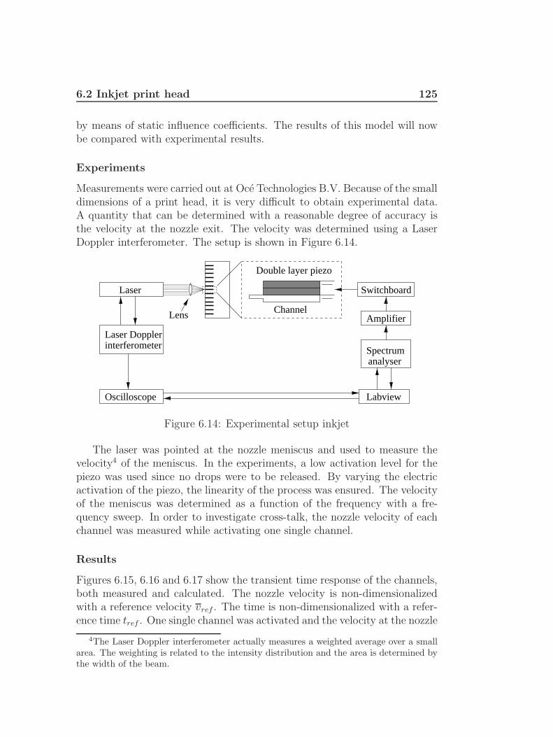
6.2 Inkjet print head 125
by means of static influence coefficients. The results of this model will nowbe compared with experimental results.
Experiments
Measurements were carried out at Oce Technologies B.V. Because of the smalldimensions of a print head, it is very difficult to obtain experimental data.A quantity that can be determined with a reasonable degree of accuracy isthe velocity at the nozzle exit. The velocity was determined using a LaserDoppler interferometer. The setup is shown in Figure 6.14.
Channel
Double layer piezo
Lens
Laser
Oscilloscope
Laser Doppler
Labview
interferometer
Switchboard
Amplifier
analyserSpectrum
Figure 6.14: Experimental setup inkjet
The laser was pointed at the nozzle meniscus and used to measure thevelocity4 of the meniscus. In the experiments, a low activation level for thepiezo was used since no drops were to be released. By varying the electricactivation of the piezo, the linearity of the process was ensured. The velocityof the meniscus was determined as a function of the frequency with a fre-quency sweep. In order to investigate cross-talk, the nozzle velocity of eachchannel was measured while activating one single channel.
Results
Figures 6.15, 6.16 and 6.17 show the transient time response of the channels,both measured and calculated. The nozzle velocity is non-dimensionalizedwith a reference velocity vref . The time is non-dimensionalized with a refer-ence time tref . One single channel was activated and the velocity at the nozzle
4The Laser Doppler interferometer actually measures a weighted average over a smallarea. The weighting is related to the intensity distribution and the area is determined bythe width of the beam.
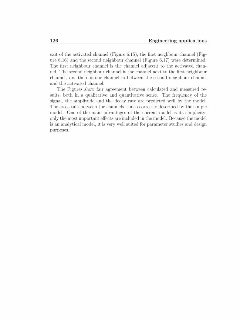
126 Engineering applications
exit of the activated channel (Figure 6.15), the first neighbour channel (Fig-ure 6.16) and the second neighbour channel (Figure 6.17) were determined.The first neighbour channel is the channel adjacent to the activated chan-nel. The second neighbour channel is the channel next to the first neighbourchannel, i.e. there is one channel in between the second neighbour channeland the activated channel.
The Figures show fair agreement between calculated and measured re-sults, both in a qualitative and quantitative sense. The frequency of thesignal, the amplitude and the decay rate are predicted well by the model.The cross-talk between the channels is also correctly described by the simplemodel. One of the main advantages of the current model is its simplicity:only the most important effects are included in the model. Because the modelis an analytical model, it is very well suited for parameter studies and designpurposes.

6.2 Inkjet print head 127
ttref
vvref
1.00.80.60.40.20
0.5
1
0
-0.5
-1
Figure 6.15: Transient response of activated channel: nozzle velocity versustime. Calculations ( ), experiments ()
ttref
vvref
1.00.80.60.40.20
0.2
0.1
0
-0.1
-0.2
Figure 6.16: Transient response of first neighbour channel: nozzle velocityversus time. Calculations ( ), experiments ()
ttref
vvref
1.00.80.60.40.20
0.2
0.1
0
-0.1
-0.2
Figure 6.17: Transient response of second neighbour channel: nozzle velocityversus time. Calculations ( ), experiments ()
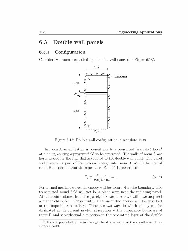
128 Engineering applications
6.3 Double wall panels
6.3.1 Configuration
Consider two rooms separated by a double wall panel (see Figure 6.18).
0.50
Excitation
B
A
0
0.49
2h
2.00
nZ = 1
Figure 6.18: Double wall configuration, dimensions in m
In room A an excitation is present due to a prescribed (acoustic) force5
at a point, causing a pressure field to be generated. The walls of room A arehard, except for the side that is coupled to the double wall panel. The panelwill transmit a part of the incident energy into room B. At the far end ofroom B, a specific acoustic impedance, Zn, of 1 is prescribed:
Zn ≡p0
ρ0c20
p
v · en= 1 (6.15)
For normal incident waves, all energy will be absorbed at the boundary. Thetransmitted sound field will not be a plane wave near the radiating panel.At a certain distance from the panel, however, the wave will have acquireda planar character. Consequently, all transmitted energy will be absorbedat the impedance boundary. There are two ways in which energy can bedissipated in the current model: absorption at the impedance boundary ofroom B and viscothermal dissipation in the separating layer of the double
5This is a prescribed value in the right hand side vector of the viscothermal finiteelement model.

6.3 Double wall panels 129
wall panel. Two different characteristics of the double wall configuration areanalysed in the present investigation: the energy dissipation in the layer andthe sound transmission through the double wall panel.
The amount of energy that is dissipated per cycle in the layer can becalculated from the net incident energy from room A and the radiated energyinto room B:
Ein =π
ωp0c0
∫At
Re p v∗ · en dAt
Erad =π
ωp0c0
∫Ab
Re p v∗ · en dAb
Ediss = Ein − Erad (6.16)
where At andAb represent the areas of the top and bottom panels respectivelyand ∗ denotes a complex conjugate.
The dissipation factor DF, the relative amount of dissipated energy, is:
DF =Ediss
Ein
= 1− Erad
Ein
(6.17)
If the viscothermal effects in the layer are neglected, the dissipation factoris evidently equal to zero. In this case there is no mechanism for energydissipation in the layer and consequently all incident energy is transmittedto room B.
The sound transmission is expressed in terms of the transmission loss,TL. The transmission loss is calculated from:
TL = 10 logPPAPPB
(6.18)
where PPA and PPB are the average quadratic pressures in room A andacross the absorbing boundary of room B respectively. The dissipation factorand the transmission loss were calculated in the frequency range from 10 to300 Hz for various configurations. The layer thickness, 2h0, and the thicknessratio between both plates of the double wall panel were varied. The totalthickness of both plates was kept equal to 3 mm. The material properties ofboth aluminium plates were as follows:
Ep = 70 · 109 N/m2 ; νp = 0.3 ; ρp = 2710 kg/m3 (6.19)
6.3.2 Finite element calculations
The finite element mesh for the calculations is shown in Figure 6.19. Thefollowing element types were used in the calculations:

130 Engineering applications
20 elements
10 elements
15 elements
Excitation
B
A
nZ = 1
Figure 6.19: Finite element mesh for the double wall configuration
• rooms A and B: standard 8 node acoustic elements HE8.ACOU
• plates: 4 node plate elements Q4.ST
• viscothermal layer: 4 node viscothermal elements Q4.VISC
• interfaces: 8 node interface elements INT.8
• impedance boundary: 4 node impedance elements Q4.IMP
Note that the problem under consideration is 2-dimensional. The finite ele-ment calculations were carried out with 3-dimensional elements. By takinga mesh with a small depth and by imposing the appropriate boundary con-ditions the 2-dimensional situation was simulated. Only 1 element was usedin the depth direction.
6.3.3 Dissipation factor
The modes of the coupled system can be divided into in-phase modes andout-of-phase modes. The in-phase modes can easily be recognized in thedissipation factor graphs because of their sharps peaks. The eigenfrequenciesof the in-phase modes are not very much affected by the presence of the airlayer. Hence, the eigenfrequency does not vary with varying layer thicknessfor these modes (see Figures 6.23, 6.24 and 6.25). When the plate thicknessis varied, the eigenfrequencies of the in-phase modes do vary, as expected(see Figures 6.20, 6.21 and 6.22).

6.3 Double wall panels 131
The broad peaks in the graphs are the out-of-phase modes. The eigen-frequencies of these modes are significantly affected by the presence of thethin air layer (see Figures 6.23, 6.24 and 6.25). Since the eigenfrequenciesare important for the behaviour of the system, the example illustrates theneed for a coupled analysis.
The graphs show that a significant amount of the incident energy is dis-sipated by viscothermal effects in the layer. This energy dissipation in thelayer is related to the pumping of air. In order to create a pumping effect, thelayer thickness and the ratio of plate thicknesses have to be chosen carefully.If the layer thickness is chosen to be very large, the viscothermal effectsare very small. If the layer thickness is very small, the coupling betweenthe two panels is so strong that no pumping effect is created. If the platethicknesses are equal, there is no pumping effect for in-phase modes. If theplate thicknesses differ greatly, the behaviour of the coupled system will bedominated by one of the plates and consequently no pumping effect occurs.These considerations show that in order to create a pumping effect, a smallgap width must be chosen while the plates are left to vibrate independently.Considering the fact that the air layer provides coupling between the panels,there might be an optimum configuration for a given situation. The presentexample shows that even the behaviour of this relatively simple configurationis a complex system of interacting factors.

132 Engineering applications
f (Hz)
DF
300250200150100500
1
0.8
0.6
0.4
0.2
0
Figure 6.20: DF versus frequency for tp1 = 1.5 mm, tp2 = 1.5 mm, 2h0 = 1mm
f (Hz)
DF
300250200150100500
1
0.8
0.6
0.4
0.2
0
Figure 6.21: DF versus frequency for tp1 = 1 mm, tp2 = 2 mm, 2h0 = 1 mm
f (Hz)
DF
300250200150100500
1
0.8
0.6
0.4
0.2
0
Figure 6.22: DF versus frequency for tp1 = 0.75 mm, tp2 = 2.25 mm, 2h0 =1 mm

6.3 Double wall panels 133
f (Hz)
DF
300250200150100500
1
0.8
0.6
0.4
0.2
0
Figure 6.23: DF versus frequency for tp1 = 1 mm, tp2 = 2 mm, 2h0 = 0.5mm
f (Hz)
DF
300250200150100500
1
0.8
0.6
0.4
0.2
0
Figure 6.24: DF versus frequency for tp1 = 1 mm, tp2 = 2 mm, 2h0 = 1 mm
f (Hz)
DF
300250200150100500
1
0.8
0.6
0.4
0.2
0
Figure 6.25: DF versus frequency for tp1 = 1 mm, tp2 = 2 mm, 2h0 = 2 mm

134 Engineering applications
6.3.4 Transmission loss
The transmission loss is shown versus the frequency in Figures 6.26 to 6.31.The graphs contain the results for the viscothermal case and the inviscid,adiabatic case 6. In this way the influence of the viscothermal effects caneasily be seen.
All Figures show that the influence of viscothermal effects is very small.Only around the eigenfrequencies there are minor differences between theresults of the calculations. It can be concluded that viscothermal effects onlyhave a very small influence on the transmission loss. This is not very surpris-ing, since in this low frequency range the transmission loss is mainly governedby the mechanical characteristics of the panels. Damping affects or controlsthe transmission loss around the eigenfrequencies and above the coincidencefrequencies of the system, i.e. the frequencies at which the structural andthe acoustic wavelengths coincide (see e.g. [98]).
Although there is no energy dissipation in the layer, there can be a hightransmission loss. It is important to distinguish between the transmissionloss and the dissipation factor. The dissipation factor relates the net inci-dent energy and the net radiated energy. The transmission loss is based onthe energy levels in the two rooms. A high energy level in a room does notimply a high net incident energy: the plate must be excited by the pressurefield. Consider for instance the case tp1 = 1 mm, tp2 = 2 mm and 2h0 = 1 mm(see Figure 6.21 and Figure 6.27). The dissipation factor shows a maximumvalue around 200 Hz. This means that almost all of the net incident energyis dissipated in the layer. The transmission loss is also high around this fre-quency, but the viscothermal effects have little influence on the transmissionloss. At this frequency the energy level in the first room is high, but only asmall portion of this energy is injected into the first plate because the pres-sure field does not excite the plate very well. In the present example theroom dimensions and the frequency range are such that the pressure field inroom A is nearly uniform.
6Inviscid and adiabatic: Γ = i and n(sσ) = γ.
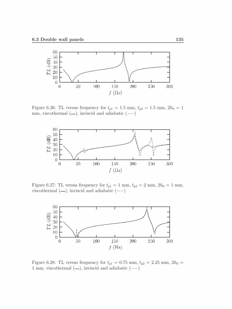
6.3 Double wall panels 135
f (Hz)
TL(dB)
300250200150100500
6050403020100
Figure 6.26: TL versus frequency for tp1 = 1.5 mm, tp2 = 1.5 mm, 2h0 = 1mm, viscothermal ( ), inviscid and adiabatic (−−)
f (Hz)
TL(dB)
300250200150100500
6050403020100
Figure 6.27: TL versus frequency for tp1 = 1 mm, tp2 = 2 mm, 2h0 = 1 mm,viscothermal ( ), inviscid and adiabatic (−−)
f (Hz)
TL(dB)
300250200150100500
6050403020100
Figure 6.28: TL versus frequency for tp1 = 0.75 mm, tp2 = 2.25 mm, 2h0 =1 mm, viscothermal ( ), inviscid and adiabatic (−−)

136 Engineering applications
f (Hz)
TL(dB)
300250200150100500
6050403020100
Figure 6.29: TL versus frequency for tp1 = 1 mm, tp2 = 2 mm, 2h0 = 0.5mm, viscothermal ( ), inviscid and adiabatic (−−)
f (Hz)
TL(dB)
300250200150100500
6050403020100
Figure 6.30: TL versus frequency for tp1 = 1 mm, tp2 = 2 mm, 2h0 = 1 mm,viscothermal ( ), inviscid and adiabatic (−−)
f (Hz)
TL(dB)
300250200150100500
6050403020100
Figure 6.31: TL versus frequency for tp1 = 1 mm, tp2 = 2 mm, 2h0 = 2 mm,viscothermal ( ), inviscid and adiabatic (−−)

6.3 Double wall panels 137
6.3.5 Practical implications
The calculations indicate that a significant amount of energy can be dissi-pated in the layer. If energy is injected into the top plate and the propertiesare adjusted in the right way, a large part of this energy can be dissipated.This implies that double wall panels with thin gas layers can be used fordamping purposes in order to reduce vibrations in which the top panel isexcited by for instance a point force or a structural member attached to theplate.
In practical situations the two plates are often connected by structuralparts: the connectors. The spacing of the connectors is important and de-serves attention. Roughly speaking, the spacing and design of the connectorsshould be such that a sufficient pumping effect can be created by the platevibrations. Trochidis [55] performed measurements on the damping charac-teristics of double wall panels with various connector spacings. He observeda maximum damping when the connector spacing was equal to a whole num-ber of structural wavelengths. The type of connection was also found to beimportant. Some types of connections allowed a larger relative motion of theplates, and higher damping values were measured in these cases. With thenewly developed techniques these phenomena can now be studied in moredetail.
Finally, the dissipation capabilities depend on the type of excitation. Fora point excitation, significant dissipation can be obtained. For a distributedload with a constant amplitude, however, the performance will be less good,because the important modes are not well excited in this case.
The presented study is a first step in the analysis of the behaviour ofdouble wall panels. As a next step investigations on the optimization ofdouble wall configurations were carried out by Basten [99] at the Universityof Twente, under contract of the Dutch Technology Foundation. The toolsthat were developed and validated within the framework of the present studywere successfully used in that research.

138 Engineering applications
6.4 Barriers in a thin layer
The calculations and measurements presented so far in this report concernedlayers with a constant thickness. In many practical applications, however,a part of the gap is blocked by obstructions. In the case of solar panels forinstance, there are two bundles of wiring that block a large part of the gap(see Figure 6.32). Chow and Pinnington [63] suggested to use obstructionsor materials in the layer to further increase the damping capabilities. Theyused porous materials in the layer for this purpose (foam and felt).
Cable bundle
Cable bundle
Figure 6.32: Cable bundles in the air layer between solar panels, top view
The main aim of the present investigation is to gain insight into the conse-quences of obstructions in the layer. Some investigations were presented con-cerning the viscothermal acousto-elastic behaviour for a non-constant layerthickness, see e.g. Onsay [69]. Onsay studied the frequency response of astrip backed by a thin gas layer with a stepwise varying layer thickness. In hisinvestigation however damping and linearity were not specifically addressed.In the present study special attention will be paid to these aspects.
6.4.1 Experimental setup
The setup with the oscillating solar panel described in chapter 4 was alsoused for the present investigation. Barriers were placed inside the layer tostudy the influence of obstructions. In Figure 6.33 a setup is shown with 4rectangular barriers in a box form. In all cases, the gap width 2h0, was equalto 12 mm: the panel spacing that is used in most solar panel configurations.The height of the barriers, 2hb, was varied. Barriers of 10.66, 10.33, 10.00,9.00 and 8.00 mm were used. Eigenfrequency and damping of the systemwere determined for each configuration for a displacement amplitude h0hof 0.3 mm. Furthermore, the linearity of the system was investigated by

6.4 Barriers in a thin layer 139
carrying out measurements at excitation amplitudes h0h ranging from 0.15mm to 0.5 mm for barriers of 10.66, 10.33 and 10.00 mm.
BarrierFixed surface
0.010
0.840
0.010
0.860
b2h0.012
Fixed surface
Panel
Figure 6.33: Barrier setup, top view (left), side view (right), dimensions inm.
6.4.2 Finite element calculations
The eigenfrequency and the damping coefficient of the system were calcu-lated with the finite element program B2000. The layer was modelled withthe new viscothermal Q4.VISC elements. The layer thickness can be spec-ified per element. In this way the barriers could easily be modelled. Theviscothermal elements were coupled to the structural Q4.ST elements withinterface elements, type INT.8. At the edges of the air layer the pressuredisturbance was set to zero: p = 0. The springs were modelled with rodelements, type R2.
The mesh density was increased around the barriers, because of the pres-sure gradients around the barriers. Three elements were used across thewidth of a barrier. Four elements with a spacing ratio of 1.5 were used tomodel the air between the barrier and the outer edge of the plate. Two timesfive elements with a spacing ratio of 1.5 were used in each direction for thearea inside the barriers. The mesh is illustrated in Figure 6.34.

140 Engineering applications
Figure 6.34: Finite element mesh for the calculations with barriers
6.4.3 Results
Linearity
The eigenfrequency of the system was not significantly affected by the am-plitude of motion (see Appendix D). The damping however increased dra-matically with increasing displacement amplitude. The damping versus am-plitude is plotted in Figures 6.35, 6.36 and 6.37 for the three barrier heights.In all cases the damping shows a nearly linear increase with amplitude. Thedamping predicted by the finite element calculations is very low comparedto the damping levels that were measured at high amplitudes. If the mea-sured damping coefficient is extrapolated to a zero displacement amplitude,the same damping coefficient is obtained as was calculated using the finiteelement model. It can be concluded that non-linearities are present thathave a large influence on the damping of the system. This is an importantobservation. In the literature, several investigations deal with the behaviourof layers with non-constant thickness. The linearity of the problem howeverwas never addressed. A physical interpretation of the phenomenon is givenin section 6.4.4.
Eigenfrequency versus barrier height
In Figure 6.38 the eigenfrequency is plotted versus the barrier height.
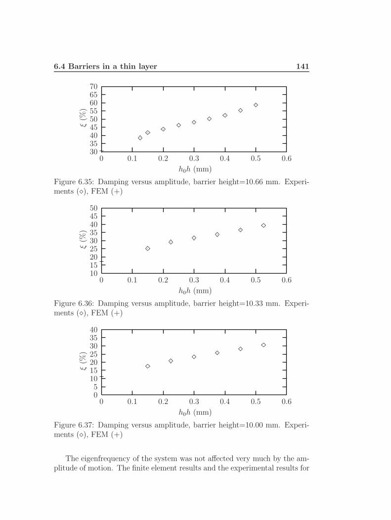
6.4 Barriers in a thin layer 141
h0h (mm)
ξ(%
)
0.60.50.40.30.20.10
706560555045403530
Figure 6.35: Damping versus amplitude, barrier height=10.66 mm. Experi-ments (), FEM (+)
h0h (mm)
ξ(%
)
0.60.50.40.30.20.10
504540353025201510
Figure 6.36: Damping versus amplitude, barrier height=10.33 mm. Experi-ments (), FEM (+)
h0h (mm)
ξ(%
)
0.60.50.40.30.20.10
4035302520151050
Figure 6.37: Damping versus amplitude, barrier height=10.00 mm. Experi-ments (), FEM (+)
The eigenfrequency of the system was not affected very much by the am-plitude of motion. The finite element results and the experimental results for

142 Engineering applications
2hb (mm)
f(H
z)
121086420
10
8
6
4
2
0
Figure 6.38: Frequency versus barrier height. Experiments (), FEM (+)
the eigenfrequency can therefore be compared. Both calculations and experi-ments show a decrease in eigenfrequency with increasing barrier height. Theexperimental frequencies are always lower than the calculated frequencies.This can mainly be attributed to the fact that the influence of the surround-ing air is neglected. The shift in eigenfrequency as a function of barrier heightis not very large and therefore the added mass remains small. The addedmass due to the surrounding air thus has a relatively large influence.
Damping versus barrier height
In Figure 6.39 the damping is plotted versus the the barrier height. The
2hb (mm)
ξ(%
)
121086420
50454035302520151050
Figure 6.39: Damping versus barrier height. Experiments (), FEM (+)

6.4 Barriers in a thin layer 143
damping shows a strong increase with increasing barrier height. By usingsimple obstructions in the layer, the damping values can be increased from3% to 40%. It was demonstrated that non-linearities are very importantin the experiments. The experimental results for an amplitude of 0.3 mm(clearly in the non-linear regime) and the calculated results (obtained with alinear model) should therefore be compared and interpreted with care. Bothcalculations and experiments predict an increase of damping with increasingbarrier height.
6.4.4 Interpretation
The experimental results show that the eigenfrequency of the system hardlyvaries with the displacement amplitude h0h. The damping however does showa linear increase with displacement amplitude. Evidently, this behaviour can-not be explained by the linear viscothermal models. There must be anothernon-linear dissipative mechanism in addition to the linear dissipative vis-cothermal effects.
Smoke was used to visualize the flow around the barriers. For large barrierheights, a vortex developed behind the barrier during the outflow stage (seeFigure 6.40).
Figure 6.40: Forming of vortex behind the barrier (side view)
The acoustic response of open tubes was studied by Disselhorst and VanWijngaarden [43], and Peters, Hirschberg, Reijen and Wijnands [44]. Intheir experiments, non-linear effects were observed related to unsteady flowseparation and the forming of vortices at the tube end. This non-lineardissipation mechanism was found to be important for small acoustic Strouhalnumbers:
Sr =ωR
vx(6.20)
where ω is the angular frequency, R is the radius of the tube and vx is theamplitude of the axial velocity at the tube end. For low acoustic Strouhal

144 Engineering applications
numbers, the dissipated energy per cycle can be calculated from [44]:
Evortex =2ρ0v
3xcdπR
2
3ω(6.21)
where cd is a parameter that is determined by the geometry of the pipeend. For a thin-walled unflanged pipe this factor is equal to 2, whereas for aflanged pipe it takes the value 13
9.
The theory that was developed for tubes will now be used to estimate theadditional energy dissipation of this mechanism for the present layer geom-etry. It must be remembered that this is a qualitative analysis, based on anorder of magnitude estimation, aimed at the identification of the dissipationmechanism. A detailed quantitative study of the non-linear separation forthe geometry under consideration would require a significant amount of workand is not within the scope of the present study.
The velocity in the thin layer that remains between the barrier and thepanel can be estimated by using the equation of continuity for incompressiblebehaviour. The amplitude of the velocity is:
v ∼= ωh0hlxblyb[2h0 − 2hb] [lxb + lyb]
(6.22)
where lxb and lyb denote the length of the barriers in the x-direction and they-direction respectively. For the present investigation lxb = 0.43 m and lyb =0.43 m (see Figure 6.33). For the three barriers of interest, the velocitiesvary between 0.4 and 12 m/s. The Reynolds number, Re = ρ0v [h0 − hb] /µ,is about 100 for the present situation. The expansion ratio, h0/ [h0 − hb],varies between 6 and 9. For the present layer geometry the acoustic Strouhalnumber can be estimated by:
Sr =ω [h0 − hb]
v(6.23)
The dimensionless velocity amplitude v was determined by using the equa-tion of continuity for incompressible behaviour. This gives using expression(6.22)7:
Sr ∼= 2 [h0 − hb]2 [lxb + lyb]
h0hlxblyb(6.24)
It can easily be verified that Sr 1. Analoguous to expression (6.21),using the appropriate total flow area, the dissipated amount of energy was
7A more accurate estimation of the velocity can be provided by using the finite elementresults, but this degree of accuracy is not relevant in the present qualitative analysis
6.4 Barriers in a thin layer 145
estimated from:
Evortex∼= 2ρ0v
3cd [2h0 − 2hb] [4lxb + 4lyb]
3ω(6.25)
Thus:
Evortex∼= 8
3ρ0cd
l3xbl3yb
[lxb + lyb]2
[h0h]3 ω2
[2h0 − 2hb]2 (6.26)
The question remains whether the amount of energy that is dissipated bythis mechanism is significant compared to the “standard” viscothermal dis-sipation. In the present study it is assumed that the dissipation mechanismsare not correlated: the dissipated energies are simply superimposed. Forthe single degree of freedom system with stiffness 8κ and viscous dampingcoefficient ξ0, the dissipated energy per cycle is given by:
Ediss = 2π8κξ0 [h0h]2 (6.27)
where κ is the stiffness of one spring and ξ0 denotes the viscous dampingcoeffient due to “standard” viscothermal effects only. The value of ξ0 canbe calculated with the finite element model. It can also be deduced fromthe experimental results by extrapolating the measured damping values to azero displacement amplitude. As stated before, the extrapolated values andthe calculated values show good agreement (see Figures 6.35, 6.36 and 6.37).An estimation shows that the energy that is dissipated by the mechanism isof the same order of magnitude as the “standard” viscothermal dissipation.This order of magnitude estimate suggests that it is the vortex mechanismthat introduces the strong non-linear damping behaviour.
In the experiments it is not possible to distinguish between the “stan-dard” linear viscothermal dissipation and the dissipation due to the non-linear mechanism. All the dissipated energy is interpreted in terms of adamping coefficient ξ according to the definition given in expression (6.27).The damping level found in the experiments can simply be calculated from:
ξ =Ediss + Evortex
2π8κ [h0h]2∼= ξ0 +
8
3
ρ0cd16πκ
l3xbl3yb
[lxb + lyb]2
[h0h]ω2
[2h0 − 2hb]2 (6.28)
This expression shows that the damping linearly increases with amplitudeh0h if all other parameters remain constant. In the experiments the dampingcoefficient showed a linear increase with amplitude and the frequency hardlyvaried with amplitude. This type of behaviour is in accordance with thevortex mechanism.
In the literature, several investigations were presented concerning theacoustic behaviour of open pipes and the flow over backward facing steps.
146 Engineering applications
Recently, and investigation was presented by Hofmans [100], dealing with anumerical and experimental study on the flow through a square-edge nozzleat low Mach number. The techniques described in this investigation wouldallow a more quantitative approach of the present problem, involving a 3Dgeometry with a driven flow. From a practical point of view, it is interest-ing to investigate if the non-linear mechanism can be used to increase thedamping performance.
The present study only concerns a qualitative analysis, based on an or-der of magnitude estimation, aimed at the identification of the dissipationmechanism. It can be concluded that the observations and this simple qual-itative analysis support the assumption that the flow separation introducesa non-linear damping behaviour.

Chapter 7
Conclusions
The general conclusions are:
• an overview was presented of linear viscothermal wave propagationmodels. Using dimensionless parameters, the models were comparedand the ranges of validity were indicated. The analysis showed thatthe low reduced frequency model is not only adequate but also themost efficient for describing viscothermal wave propagation;
• the low reduced frequency model was validated with specially designedexperiments. The experiments enabled accurate measurements andprovided new detailed information. The agreement between theoryand experiment was good;
• a new viscothermal acoustic finite element was developed, based onthe low reduced frequency model. The new element can be coupledto structural elements, enabling fully coupled calculations for complexgeometries. The finite element model was validated with experiments.Calculations and experiments showed fair agreement. Thus, a new andefficient simulation tool has been developed for describing of viscother-mal wave propagation, including acousto-elastic interaction;
• the new tools were succesfully used in a number of practical applica-tions: the behaviour of an array of folded solar panels during launch,the design of an inkjet print head and the behaviour of double wallpanels.

148 Conclusions

Bibliography
[1] F. Augusztinovicz. Calculation of noise control by numerical methods- what we can do and what we cannot do - yet. In InterNoise 97, pages27–42, Budapest, Hungary, 1997.
[2] Course on advanced techniques in applied and numerical acoustics. InP.Sas, editor, ISAAC 7, Leuven, Belgium, 1996. K.U. Leuven.
[3] H. Tijdeman. On the propagation of sound waves in cylindrical tubes.Journal of Sound and Vibration, 39:1–33, 1975.
[4] C. Karra, M.B. Tahar, G. Marquette, and M.T. Chau. Boundary el-ement analysis of problems of acoustic propagation in viscothermalfluid. In F. Allison Hill and R. Lawrence, editors, InterNoise 96, pages3003–3006, Liverpool, United Kingdom, 1996. Institute of Acoustics.
[5] C. Karra and M. Ben Tahar. An integral equation formulation for boun-dary element analysis of propagation in viscothermal fluids. Journal ofthe Acoustical Society of America, 102(3):1311–1318, 1997.
[6] J.W.S. Rayleigh. The Theory of Sound, volume II. Dover publications,second, revised edition, 1945.
[7] W.S. Griffin, H.H. Richardson, and S. Yamanami. A study of fluidsqueeze-film damping. Journal of Basic Engineering, pages 451–456,1966.
[8] S.M.R. Hashemi and B.J. Roylance. Analysis of an oscillatory oilsqueeze film including effects of fluid inertia. Tribology Transactions,32:461–468, 1989.
[9] E.C. Kuhn and C.C. Yates. Fluid inertia effect on the film pressurebetween axially oscillating parallel circular plates. ASLE Transactions,7:299–303, 1964.

150 BIBLIOGRAPHY
[10] J. Prakash and H. Christensen. Squeeze film between two rough rectan-gular plates. Journal of Mechanical Engineering Science, 20:183–188,1978.
[11] P. Sinha and C. Singh. Micropolar squeeze films between rough rect-angular plates. Applied Scientific Research, 39:169–179, 1982.
[12] R.M. Terrill. The flow between two parallel circular discs, one of whichis subject to a normal sinusoidal oscillation. Journal of LubricationTechnology, pages 126–131, 1969.
[13] J.A. Tichy and M.F. Modest. Squeeze film flow between arbitrarytwo-dimensional surfaces subject to normal oscillations. Journal ofLubrication Technology, 100:316–322, 1978.
[14] J.A. Tichy. Measurements of squeeze-film bearing forces and pressures,including the effect of fluid inertia. ASLE Transactions, 28:520–526,1984.
[15] J.V. Beck, W.G. Holliday, and C.L. Strodtman. Experiments and anal-ysis of a flat disk squeeze-film bearing including effects of supportedmass motion. Journal of Lubrication Technology, pages 138–148, 1969.
[16] V. Ramamurthy and U.S. Rao. The steady streaming generated by avibrating plate parallel to a fixed plate in a dusty fluid. Fluid DynamicsResearch, 2:47–63, 1987.
[17] C.Y. Wang and B. Drachman. The steady streaming generated by avibrating plate parallel to a fixed plate. Applied Scientific Research,39:55–68, 1982.
[18] N. Rott. The influence of heat conduction on acoustic streaming. Jour-nal of Applied Mathematics and Physics, 25:417, 1974.
[19] P. Merkli and H. Thomann. Transition to turbulence in oscillating pipeflow. Journal of Fluid Mechanics, 68:567–575, 1975.
[20] G. Maidanik. Energy dissipation associated with gas-pumping in struc-tural joints. Journal of the Acoustical Society of America, 40:1064–1072, 1966.
[21] E.E. Ungar and J.R. Carbonell. On panel vibration damping due tostructural joints. AIAA Journal, 4:1385–1390, 1966.

BIBLIOGRAPHY 151
[22] S. Makarov and M. Ochmann. Non-linear and thermoviscous phenom-ena in acoustics, part I. Acustica, 82:579–606, 1996.
[23] S. Makarov and M. Ochmann. Non-linear and thermoviscous phenom-ena in acoustics, part II. Acustica, 83:197–222, 1997.
[24] S. Makarov and M. Ochmann. Non-linear and thermoviscous phenom-ena in acoustics, part III. Acustica, 83:827–846, 1997.
[25] G.P.J. Too and S.T. Lee. Thermoviscous effects on transient andsteady-state sound beams using non-linear progressive wave equationmodels. Journal of the Acoustical Society of America, 97:867–874, 1995.
[26] H.A. Scarton and W.T. Rouleau. Axisymmetric waves in compress-ible Newtonian liquids contained in rigid tubes: steady-periodic modeshapes and dispersion by the method of eigenvalleys. Journal of FluidMechanics, 58:595–621, 1973.
[27] K. Rathnam and M.M. Oberai. Acoustic wave propagation in cylin-drical tubes containing slightly rarefied gases. Journal of Sound andVibration, 60:379–388, 1978.
[28] K. Rathnam. Influence of velocity slip and temperature jump in rarefiedgas acoustic oscillations in cylindrical tubes. Journal of Sound andVibration, 103:448–452, 1985.
[29] M. Moldover, J. Mehl, and M. Greenspan. Gas-filles spherical res-onators: theory and experiment. Journal of the Acoustical Society ofAmerica, 79:253–270, 1986.
[30] M.J. Anderson and P.G. Vaidya. Sound propagation in a waveguidewith finite thermal conduction at the boundary. Journal of the Acous-tical Society of America, 86:2385–2396, 1989.
[31] H.S. Roh, W.P Arnot, and J.M. Sabatier. Measurements and calcula-tion of acoustic propagation constants in arrays of small air-filled rect-angular tubes. Journal of the Acoustical Society of America, 89:2617–2624, 1991.
[32] N. Rott. Damped and thermally driven acoustic oscillations. Journalof Applied Mathematics and Physics, 20:230, 1969.
[33] N. Rott. Thermally driven acoustic oscillations, part II: stability limitfor helium. Journal of Applied Mathematics and Physics, 24:24, 1973.

152 BIBLIOGRAPHY
[34] N. Rott. Thermally driven acoustic oscillations, part III: second-orderheat flux. Journal of Applied Mathematics and Physics, 26:43, 1975.
[35] N. Rott and G. Zouzoulas. Thermally driven acoustic oscillations, partIV: tubes with variable cross-section. Journal of Applied Mathematicsand Physics, 27:197, 1976.
[36] G. Zouzoulas and N. Rott. Thermally driven acoustic oscillations, partV: gas-liquid oscillations. Journal of Applied Mathematics and Physics,27:325, 1976.
[37] R. Raspet, H.E. Bass, and J. Kordomenos. Thermoacoustics of trav-elling waves: theoretical analysis for an inviscid ideal gas. Journal ofthe Acoustical Society of America, 94:2232–2239, 1993.
[38] J. Kordomenos, A.A. Atchley, R. Raspet, and H.E. Bass. Experimen-tal study of a thermoacoustic termination of a travelling-wave tube.Journal of the Acoustical Society of America, 98:1623–1628, 1995.
[39] E. Stuhltrager and H. Thomann. Oscillations of a gas in an open-endedtube near resonance. Journal of Applied Mathematics and Physics,37:155, 1986.
[40] J.H.M. Disselhorst. Acoustic resonance in open tubes. PhD thesis,University of Twente, The Netherlands, 1978.
[41] M.P. Verge. Aeroacoustics of confined jets. PhD thesis, TechnicalUniversity of Eindhoven, The Netherlands, 1995.
[42] U. Ingard. Acoustic non-linearity of an orifice. Journal of the AcousticalSociety of America, 42, 1967.
[43] J.H.M. Disselhorst and L. van Wijngaarden. Flow in the exit of openpipes during acoustic resonance. Journal of Fluid Mechanics, 99:293–319, 1980.
[44] C.A.M. Peters, A. Hirschberg, A.J. Reijen, and A.P.J. Wijnands.Damping and reflection coefficient measurements for an open pipe atlow Mach and low Helmholtz numbers. Journal of Fluid Mechanics,256:499–534, 1993.
[45] M. Bruneau, Ph. Herzog, J. Kergomard, and J.D. Polack. Generalformulation of the dispersion equation in bounded visco-thermal fluid.Wave Motion, 11:441–451, 1989.

BIBLIOGRAPHY 153
[46] J.B. Mehl. Spherical acoustic resonator: effects of shell motion. Journalof the Acoustical Society of America, 78:782–788, 1985.
[47] G. Plantier and M. Bruneau. Heat conduction effects on the acousticresponse of a membrane separated by a very thin air film from a backingelectrode. Journal Acoustique, 3:243–250, 1990.
[48] M. Bruneau, A.M. Bruneau, and P. Hamery. An improved approachto modelling the behaviour of thin fluid films trapped between a vi-brating membrane and a backing wall surrounded by a reservoir at theperiphery. Acustica, 1:227–234, 1993.
[49] P. Hamery, M. Bruneau, and A.M. Bruneau. Mouvement d’une couchede fluide dissipatif en espace clos sous l’action d’une source etendue.Journal de Physique IV, 4:C5–213–C5–216, 1994. (in French).
[50] C. Karra. Private communication, 1996.
[51] M. Bruneau, J.D. Polack, Ph. Herzog, and J. Kergomard. Formula-tion generale des equations de propagation et de dispersion des ondessonores dans les fluides viscothermiques. Colloque de Physique, 51:C2–17–C2–20, 1990. (In French).
[52] M. Bruneau. Acoustique des cavites: modeles et applications. Journalde Physique IV, 4:C5–675–C5–684, 1994. (in French).
[53] A.M. Bruneau, M. Bruneau, Ph. Herzog, and J. Kergomard. Boundarylayer attenuation of higher order modes in waveguides. Journal ofSound and Vibration, 119:15–27, 1987.
[54] P.N. Liang and H.A. Scarton. Three-dimensional mode shapes forhigher order circumferential thermoelastic waves in an annular elas-tic cylinder. Journal of Sound and Vibration, 177:121–135, 1994.
[55] A. Trochidis. Vibration damping due to air or liquid layers. Acustica,51:201–212, 1982.
[56] A. Trochidis. Korperschalldampfung durch Viscositatsverluste in Gass-chichten bei Doppelplatten. PhD thesis, ITA Berlin, 1977. (In German).
[57] M. Moser. Damping of structure born sound by the viscosity of a layerbetween two plates. Acustica, 46:210–217, 1980.
154 BIBLIOGRAPHY
[58] W.M. Beltman, P.J.M. van der Hoogt, R.M.E.J. Spiering, and H. Ti-jdeman. Energy dissipation in thin air layers. In P. Sas, editor, ISMA21 Conference on Noise and Vibration Engineering, pages 1605–1618,Leuven, Belgium, 1996. Katholieke universiteit Leuven.
[59] W.M. Beltman, P.J.M. van der Hoogt, R.M.E.J. Spiering, and H. Ti-jdeman. Implementation and experimental validation of a new vis-cothermal acoustic finite element for acousto-elastic problems. Journalof Sound and Vibration, 1998. (accepted for publication).
[60] R.M.S.M. Schulkes. Interactions of an elastic solid with a viscous fluid:eigenmode analysis. Technical Report 90-46, Delft University of Tech-nology, Faculty of Technical Mathematics and Informatics, Delft, TheNetherlands, 1990.
[61] R.M.S.M. Schulkes. Fluid oscillations in an open, flexible container.Technical Report 89-69, Delft University of Technology, Faculty ofTechnical Mathematics and Informatics, Delft, The Netherlands, 1989.
[62] L.C. Chow and R.J. Pinnington. Practical industrial method of increas-ing structural damping in machinery, I: squeeze film damping with air.Journal of Sound and Vibration, 118:123–139, 1987.
[63] L.C. Chow and R.J. Pinnington. Practical industrial method of in-creasing structural damping in machinery, II: squeeze film dampingwith liquids. Journal of Sound and Vibration, 128:333–347, 1989.
[64] M.R. Stinson. The propagation of plane sound waves in narrow andwide circular tubes, and generalization to uniform tubes of arbitrarycross-section. Journal of the Acoustical Society of America, 89:550–558,1991.
[65] A. Cummings. Sound propagation in narrow tubes of arbitrary cross-section. Journal of Sound and Vibration, 162:27–42, 1993.
[66] A.D. Lapin. Integral relations for acoustic modes in a channel witharbitrary cross-section. Acoustical Physics, 42:509–511, 1996.
[67] M.J.H. Fox and P.N. Whitton. The damping of structural vibrationsby thin gas films. Journal of Sound and Vibration, 73:279–295, 1980.
[68] T. Onsay. Effects of layer thickness on the vibration response of aplate-fluid layer system. Journal of Sound and Vibration, 163:231–259,1993.

BIBLIOGRAPHY 155
[69] T. Onsay. Dynamic interaction between the bending vibrations of aplate and a fluid layer attenuator. Journal of Sound and Vibration,178:289–313, 1994.
[70] W.M. Beltman, P.J.M. van der Hoogt, R.M.E.J. Spiering, and H. Tij-deman. Air loads on a rigid plate oscillating normal to a fixed surface.Journal of Sound and Vibration, 206(3):217–241, 1997.
[71] W.M. Beltman, P.J.M. van der Hoogt, R.M.E.J. Spiering, and H. Ti-jdeman. Air loads on solar panels during launch. In W.R. Burke,editor, Conference on Spacecraft Structures, Materials and MechanicalTesting, pages 219–226, Noordwijk, The Netherlands, 1996. EuropeanSpace Agency. ESA SP-386.
[72] W.M. Beltman. Damping of double wall panels. Journal of the DutchAcoustical Society (NAG), 131:27–38, 1996. (in Dutch).
[73] M. Bruneau, A.M. Bruneau, Z. Skvor, and P. Lotton. An equivalentnetwork modelling the strong coupling between a vibrating membraneand a fluid film. Acustica, 2:223–232, 1994.
[74] J.B. Mehl. Acoustic resonance frequencies of deformed spherical res-onators. Journal of the Acoustical Society of America, 71:1109–1113,1982.
[75] J.B. Mehl. Acoustic resonance frequencies of deformed spherical res-onators, II. Journal of the Acoustical Society of America, 79:278–285,1986.
[76] M. Abramowitz and I.A. Stengun. Handbook of mathematical functions.Dover publications, seventh Dover printing edition.
[77] P.M. Morse and H. Feshbach. Methods of theoretical physics. McGraw-Hill, 1953.
[78] P.N. Liang and H.A. Scarton. Attenuation of higher order circumferen-tial thermoacoustic waves in viscous fluid lines. Journal of Sound andVibration, 193:1099–1113, 1996.
[79] H. Hudde. The propagation constant in lossy circular tubes near thecutoff frequencies of higher order modes. Journal of the AcousticalSociety of America, 83:1311–1318, 1988.

156 BIBLIOGRAPHY
[80] J. Kergomard, M. Bruneau, A.M. Bruneau, and Ph. Herzog. On thepropagation constant of higher order modes in a cylindrical waveguide.Journal of Sound and Vibration, 126:178–181, 1988.
[81] Computational Applications and System Integration Inc, 2004 S.Wright Street, Urbana, IL 61821, USA. Ansys User Manual, 5.3 edi-tion, 1996.
[82] W. Kay Meyerhoff. Added masses of thin rectangular plates calculatedfrom potential theory. Journal of Ship Research, pages 100–111, 1970.
[83] M.D. McCollum and C.M. Siders. Modal analysis of a structure in acompressible fluid using a finite element/boundary element approach.Journal of the Acoustical Society of America, 99(4):1949–1957, 1996.
[84] F.P. Grooteman. Coupled acousto-elastic analysis; theory and imple-mentation in the finite element program B2000. Technical Report NLRCR 94218 L, National Aerospace Laboratory, The Netherlands, 1994.(restricted).
[85] S. Merazzi. Modular finite element analysis tools applied to problems inengineering. PhD thesis, EPFL Lausanne Nr. 1251, Switserland, 1994.
[86] E.H. Dowell, G.F. Gorman, and D.A. Smith. Acousto-elasticity: gen-eral theory, acoustic natural modes and forced response to sinusoidalexcitation, including comparisons with experiment. Journal of Soundand Vibration, 52:519–542, 1977.
[87] R.D. Blevins. Formulas for natural frequencies and mode shapes. VanNostrand Reinhold, first edition, 1979.
[88] H.T. Koelink, H. Schippers, J.J. Heijstek, and J.J Derksen. Modalanalysis of solar panels using boundary integral equations. TechnicalReport NLR TP 92281 L, National Aerospace Laboratory, The Nether-lands, 1992.
[89] P.E. Harrewijne. The influence of air on the eigenfrequencies of a solararray. Technical Report WFW 93.107, Technical University of Eind-hoven, Eindhoven, The Netherlands, 1993.
[90] F.P. Grooteman and H. Schippers. Coupled analysis in acoustics on thedynamical behaviour of solar arrays. In P. Sas, editor, ISMA 19 Con-ference on Noise and Vibration Engineering, pages 101–124, Leuven,Belgium, 1994. Katholieke universiteit Leuven.

BIBLIOGRAPHY 157
[91] J.J. Wijker. Acoustic effects on the dynamics of lightweight structures.Technical report, Fokker Space, Leiden, The Netherlands.
[92] P. Santini, F. Morganti, and R. Giovannucci. Acoustics of space struc-tures. In North Atlantic Treaty Organization, editor, Symposium onImpact of Acoustic Loads on Aircraft Structures, pages 9A–1–9A–13,Lillehammer, Norway, 1994. AGARD-CP-549.
[93] B.W. Kooi. Air effects on the dynamic behaviour of stowed solar ar-ray wings. Technical Report FSS-R-87-134 (restricted), Fokker Space,Leiden, The Netherlands, 1987.
[94] J.F. Dijksman. Hydrodynamics of small tubular pumps. Journal ofFluid Mechanics, 139:173–191, 1984.
[95] J.D. Beasly. Model for fluid ejection and refill in an impulsive drivejet. Photographic Science and Engineering, 21:78–82, 1977.
[96] D.F. Elger. An experimental and analytical study of the internal fluiddynamics of an inkjet print head. PhD thesis, Oregon State University,United States of America, 1986.
[97] D.F. Elger and R.L. Adams. Some notes on inkjet print head design.Industrial Applications of Fluid Mechanics, pages 51–54, 1987.
[98] D.A. Bies and C.H. Hansen. Engineering Noise Control. E&FN Spon,second edition, 1996.
[99] T.G.H. Basten, W.M. Beltman, and H. Tijdeman. Optimizationof viscothermal damping of double wall panels. In InterNoise 98,Christchurch, New Zealand, 1998.
[100] G.C.J. Hofmans. Vortex sound in confined flows. PhD thesis, TechnicalUniversity of Eindhoven, The Netherlands, 1998.

158 BIBLIOGRAPHY
Appendix A
Nomenclature
A function describing velocity and temperature profilesAq, Bq participation factorsAaq, Baq, Ahq, Bhq constants
Acd
cross-sectional areaAcd dimensionless cross-sectional area∂Acd dimensionless area of cross-section boundary
Apd
propagation direction area
∂Apd
area of propagation direction boundaryB(s) function accounting for viscous or thermal effects
a = lylx
aspect ratio
C function describing the temperature profileC1, C2, C3, C4 constantsCp specific heat at constant pressureCv specific heat at constant volumec0 undisturbed speed of soundcd non-linear dissipation factorceff effective speed of soundD function describing the temperature profileDF dissipation factor
Dp =Ept3p12
bending stiffnessEp Young’s modulus of plate materialEt Young’s modulus of top layerEb Young’s modulus of bottom layer
160 Nomenclature
Ediss dissipated energy per cycleEin incident energy per cycleElay energy stored in the air layerEp energy stored in plateErad radiated energy per cycleEvortex dissipated energy per cycle by vortex mechanismen unit normal vectorer unit vector in the r-directionex unit vector in the x-directioney unit vector in the y-directionez unit vector in the z-directioneθ unit vector in the θ-directioneφ unit vector in the φ-directionF ex excitation forceF gap force due to the pressure distribution in the gapF gap spring forcefm function describing wave propagation in tubesH transfer functionh0 half-layer thicknesshb dimensionless displacement of top springs, half-barrier heighthn half-nozzle heightht dimensionless displacement of bottom springsI area moment of inertiai =√−1 imaginary unit
J torsion constantjn spherical Bessel function of order nJm Bessel function of the first kind, order mk = ωl
c0reduced frequency
ka acoustic wave numberkaq = k2
a − k2q wave number
kar =√k2a + k2Γ2 wave number
kb stiffness of bottom springkb dimensionless stiffness of bottom springkh entropic wave numberkhq = k2
h − k2q wave number
khr =√k2h + k2Γ2 wave number
kp plate elastic wave numberkp1 = kkp wave number
kp2 =√is2 + k2k2
p wave number

Nomenclature 161
kq wave numberkr = ωR
c0wave number in the r-direction
kt stiffness of top springkt dimensionless stiffness of top springkx = ωlx
c0wave number in the x-direction
kv rotational wave numberkvq = k2
v − k2q wave number
l characteristic length scaleln half length of nozzlelx half length in the x-directionlxb half barrier length in the x-directionly half length in the y-directionlyb half barrier length in the y-directionlz half length in the z-directionm mass, order of circumferential harmonic wavesm′ mass per unit lengthn(sσ) polytropic constantp = p0 [1 + peiωt] pressurep0 mean pressurep dimensionless pressure amplitudepi = p0 [1 + pie
iωt] incident pressure on membranepi dimensionless incident pressure amplitudep1 pressure in point 1p2 pressure in point 2p3 pressure in point 3PPA average quadratic pressure in room APPB average quadratic pressure across absorbing boundary of room BR radius< squeeze termR0 gas constantr radial co-ordinater dimensionless radial co-ordinateSr acoustic Strouhal number
s = l√
ρ0ωµ
shear wave number
T = T0 [1 + Teiωt] temperatureT0 mean temperatureT dimensionless temperature amplitudeTa acoustic temperatureTh entropic temperatureTm membrane tensionTL transmission loss

162 Nomenclature
t timetb thickness of bottom layertm membrane thicknesstp plate thicknesstp1 thickness plate 1tp2 thickness plate 2tref reference timett thickness of top layerv = c0ve
iωt velocity vectorv dimensionless amplitude of the velocity vectorv dimensionless amplitude of the velocityvl solenoidal velocity vectorvla acoustic part of solenoidal velocity vectorvlh entropic part of solenoidal velocity vectorvv rotational velocity vectorvm = c0vme
iωt membrane velocity< vm > average membrane velocityvm dimensionless membrane velocityvp plate velocityvp dimensionless plate velocityvr dimensionless velocity component in the r-directionvref reference velocityvx dimensionless velocity component in the x-directionvxn nozzle velocity in the x-directionvxn dimensionless nozzle velocity in the x-directionvy dimensionless velocity component in the y-directionvz dimensionless velocity component in the z-directionvθ dimensionless velocity component in the θ-directionvφ dimensionless velocity component in the φ-directionvcd velocity vector in the cd-directionsvpd velocity vector in the pd-directionsW1,W2 constantsx = lxx x-co-ordinatex dimensionless x-co-ordinatex spatial co-ordinatesxcd cross-sectional co-ordinatesxpd propagation co-ordinatesy = lyy y-co-ordinateY mobility functionYmn spherical harmonic functiony dimensionless y-co-ordinate

Nomenclature 163
z = h0z z-co-ordinateZ membrane impedanceZ0 reference level for the impedanceZi imaginary part of membrane impedanceZn specific normal acoustic impedanceZr real part of membrane impedancez dimensionless z-co-ordinate
α rotation angleΓ propagation constant
γ = CpCv
ratio of specific heats
ε = ρ0h0
ρptpratio of mass per unit area
η bulk viscosityθ co-ordinate in the θ-directionθ dimensionless co-ordinate in the θ-directionΛa constantΛh constantλ thermal conductivityµ dynamic viscosityξ viscosity ratio, dimensionless damping coefficientξ0 dimensionless damping coefficient for linear viscothermal dampingνp Poisson’s ratio of plate materialρ = ρ0 [1 + ρeiωt] densityρ0 mean density of airρ dimensionless density amplitudeρm density of membrane materialρp density of plate material
σ =√
µCpλ
square root of the Prandtl number
Φ viscous dissipation functionφ co-ordinate in the φ-directionφ dimensionless co-ordinate in the φ-directionΩ dimensionless frequencyω angular frequency

164 Nomenclature
∇ gradient operator∇ dimensionless gradient operator∇cd dimensionless gradient operator in the cd-directions∇pd dimensionless gradient operator in the pd-directions∆ Laplace operator∆ dimensionless Laplace operator∆cd dimensionless Laplace operator in the cd-directions∆r dimensionless Laplace operator in the r-directionζ loss factor∗ complex conjugate
[Ka] acoustic stiffness matrix[Ka
]acoustic stiffness matrix for the inviscid, adiabatic case
[Kc] coupling matrix[Ks] structural stiffness matrix[Ma(s)] acoustic mass matrix[Ma
]acoustic mass matrix for the inviscid, adiabatic case
[M c(s)] coupling matrix[M c
]coupling matrix for the inviscid, adiabatic case
[Ms] structural mass matrix[Na] acoustic interpolation functions[Ns] structural interpolation functions[Φa]
matrix with uncoupled acoustic modes for the inviscid, adiabatic case
[Φs] matrix with uncoupled structural modes[Ωa]
diagonal acoustic eigenvalue matrix for the inviscid, adiabatic case
[Ωs] diagonal structural eigenvalue matrix
F ext external force vectorF ext
external force vector for the inviscid, adiabatic case
P vector with pressure degrees of freedomU vector with structural degrees of freedomηa vector with generalized acoustic co-ordinatesηs vector with generalized structural co-ordinates

Appendix B
Geometries, co-ordinatesystems and functions
B.1 Sphere
R r
θ
φ
Figure B.1: Geometry of sphere
The basic geometrical dimensions and operators are:
l = R ; x = (r, θ, φ)
r =r
R; θ = θ ; φ = φ
∇ = er∂
∂r+ eθ
1
r
∂
∂θ+ eφ
1
r sin (θ)
∂
∂φ(B.1)
∆ =1
r2
∂
∂r
[r2 ∂
∂r
]+
1
r2 sin (θ)
∂
∂θ
[sin (θ)
∂
∂θ
]+
1
r2 sin (θ)
∂2
∂φ2

166 Geometries, co-ordinate systems and functions
B.2 Circular tube
R
θ
r
x
Figure B.2: Geometry of circular tube
The basic geometrical dimensions and operators are:
l = R ; x = (r, θ, x)
r =r
R; θ = θ ; x =
ωx
c0
∇ = er∂
∂r+ eθ
1
r
∂
∂θ+ exk
∂
∂x(B.2)
∆ =∂2
∂r2+
1
r
∂
∂r+
1
r2
∂2
∂θ2+ k2 ∂
2
∂x2
The operators for the low reduced frequency model are:
xcd = (r, θ) ; xpd = (x)
∇cd = er∂
∂r+ eθ
1
r
∂
∂θ; ∇pd = exk
∂
∂x(B.3)
∆cd =∂2
∂r2+
1
r
∂
∂r+
1
r2
∂2
∂θ2; ∆pd = k2 ∂
2
∂x2
The functions that are used in the low reduced frequency model are given inTable B.1.

B.2 Circular tube 167
Total Low s High s
AJ0
(sri√i)
J0
(si√i) − 1 −1
4is2
[1− r2
]−1
BJ2
(si√i)
J0
(si√i) −1
8is2 −1
< 1
π
∫ 2π
θ=0vr(x, 1, θ)dθ
Table B.1: Expressions for circular tube

168 Geometries, co-ordinate systems and functions
B.3 Rectangular tube
yly
x lz
zl
zl
y
Figure B.3: Geometry of rectangular tube
The basic geometrical dimensions and operators are:
l = ly ; x = (x, y, z) ; a =lzly
x =ωx
c0; y =
y
ly; z =
z
ly
∇ = exk∂
∂x+ ey
∂
∂y+ ez
∂
∂z(B.4)
∆ = k2 ∂2
∂x2+
∂2
∂y2+
∂2
∂z2
The operators for the low reduced frequency model are:
xcd = (y, z) ; xpd = (x)
∇cd = exk∂
∂x; ∇pd = ey
∂
∂y+ ez
∂
∂z(B.5)
∆cd =∂2
∂y2+
∂2
∂z2; ∆pd = k2 ∂
2
∂x2
The functions that are used in the low reduced frequency model are given intable B.2.

B.3
Recta
ngula
rtu
be
169
Total Low s High s
A Q1
∞∑q=1,3...
−1q−1
2
qQ22
[cosh (Q2z)
cosh (Q2)− 1
]cos
(qπy
2
)Q1
∞∑q=1,3...
−1q−1
2
qQ22
cosh(Q2z
)cosh
(Q2
) − 1
cos(qπy
2
)−1
Q1 =ia2s24
π; Q2 = a
√(qπ
2
)2
+ is2 Q1 =ia2s24
π; Q2 = a
qπ
2
B Q1
∞∑q=1,3...
−1q−1
2
q2Q22
[tanh (aQ2)
aQ2
− 1
]Q1
∞∑q=1,3...
−1q−1
2
q2Q22
tanh(aQ2
)aQ2
− 1
−1
Q1 =ia2s28
π2; Q2 = a
√(qπ
2
)2
+ is2 Q1 =ia2s28
π2; Q2 = a
qπ
2
< 1
4
∫ 1
z=−1[vy(x, 1, z)− vy(x,−1, z)] dz +
1
4
1
a
∫ 1
y=−1[vz(x, y, 1)− vz(x, y,−1)] dy
Table B.2: Expressions for rectangular tube

170 Geometries, co-ordinate systems and functions
B.4 Circular layer
R
r
zh
θ 0
0
h
Figure B.4: Geometry of the circular layer
The basic geometrical dimensions and operators are:
l = h0 ; x = (r, θ, z)
r =ωr
c0
; θ = θ ; z =z
h0
∇ = erk∂
∂r+ eθk
1
r
∂
∂θ+ ez
∂
∂z(B.6)
∆ = k2 ∂2
∂r2+ k2 1
r
∂
∂r+ k2 1
r2
∂2
∂θ2+
∂2
∂z2
The operators for the low reduced frequency model are:
xcd = (z) ; xpd = (r, θ)
∇cd = ez∂
∂z; ∇pd = erk
∂
∂r+ eθk
1
r
∂
∂θ(B.7)
∆cd =∂2
∂z2; ∆pd = k2 ∂
2
∂r2+ k2 1
r
∂
∂r+ k2 1
r2
∂2
∂θ2
The functions that are used in the low reduced frequency model are given intable B.3.

B.4 Circular layer 171
Total Low s High s
Acosh
(sz√i)
cosh(s√i) − 1
1
2is2
[1
3z2 − 1
]−1
Btanh
(s√i)
s√i
− 1 −1
3is2 −1
< 1
2[vz(x, y, 1)− vz(x, y,−1)]
Table B.3: Expressions for the circular layer

172 Geometries, co-ordinate systems and functions
B.5 Rectangular layer
0
yly
h
l
hxl
lx 0
yx
z
Figure B.5: Geometry of the rectangular layer
The basic geometrical dimensions and operators are:
l = h0 ; x = (x, y, z) ; a =lylx
x =ωx
c0; y =
ωy
c0; z =
z
h0
∇ = exk∂
∂x+ eyk
∂
∂y+ ez
∂
∂z(B.8)
∆ = k2 ∂2
∂x2+ k2 ∂
2
∂y2+
∂2
∂z2
(B.9)
The operators for the low reduced frequency model are:
xcd = (z) ; xpd = (x, y)
∇cd = ez∂
∂z; ∇pd = exk
∂
∂x+ eyk
∂
∂y(B.10)
∆cd =∂2
∂z2; ∆pd = k2 ∂
2
∂x2+ k2 ∂
2
∂y2
The functions that are used in the low reduced frequency model are given intable B.4.

B.5 Rectangular layer 173
Total Low s High s
Acosh
(sz√i)
cosh(s√i) − 1
1
2is2
[1
3z2 − 1
]−1
Btanh
(s√i)
s√i
− 1 −1
3is2 −1
< 1
2[vz(x, y, 1)− vz(x, y,−1)]
Table B.4: Expressions for the rectangular layer

174 Geometries, co-ordinate systems and functions

Appendix C
Numerical solution procedures
C.1 The spherical resonator
As an example, the eigenfrequencies of a spherical resonator are calculated.The equation of interest is:
[1− αh
αa
] n(n+ 1)
1 +1
jn (kv)
∂jn (kvr)
∂r
∣∣∣∣∣1
= (C.1)
1
jn (ka)
∂jn (kar)
∂r
∣∣∣∣∣1
−(αhαa
)1
jn (kh)
∂jn (khr)
∂r
∣∣∣∣∣1
The partial derivatives of the spherical Bessel functions are:
∂jn (kar)
∂r= ka
[jn−1 (kar)−
(n+ 1
kar
)jn (kar)
](C.2)
The equation for the eigenfrequencies can now be written as:
[1− αh
αa
] n(n+ 1)
1 + kv
jn−1 (kv)
jn (kv)−(n+ 1
kv
) = (C.3)
ka
[jn−1 (ka)
jn (ka)−(n+ 1
ka
)]− αhαakh
[jn−1 (kh)
jn (kh)−(n+ 1
kh
)]
For very large values of the imaginary part of the argument, the value of thespherical Bessel functions becomes very large. This causes problems in the
176 Numerical solution procedures
numerical solution of the equation. The spherical Bessel functions can bewritten as:
j0 (kar) =sin (kar)
kar
j1 (kar) =sin (kar)
(kar)2 −
cos (kar)
(kar)
j2 (kar) =
(3
(kar)3 −
1
kar
)sin (kar)−
3
(kar)2 cos (kar) (C.4)
jn+1 (kar) =(
2n+ 1
kar
)jn (kar)− jn−1 (kar)
In order to avoid problems for large values of the imaginary part of the ar-gument, the appropriate component was removed from the ratio of Besselfunctions by dividing both the numerator and the denonimator by this ex-ponential component. The eigenfrequencies were obtained using a simplefunction minimization procedure in the program MatLab. However, the so-lution procedure required some care. For the present test case, the ratiobetween the real and the imaginary parts of the frequency is of the orderof 103 to 106. The minimization procedure in MatLab is able to minimizea scalar function of multiple variables. The real part of the function to beminimized is mainly related to the real part of the frequency, whereas theimaginary part of the function is mainly determined by the imaginary com-ponent of the frequency. As for the frequency, the real and the imaginaryparts of the function are of a different order of magnitude. Minimizing theabsolute value of the function is therefore not a good approach, since thisapproach is relatively insensitive to changes in the imaginary part of the fre-quency. Therefore another strategy was adopted. First, the (square of the)real part of the function was minimized with the real part of the frequency asthe minimization variable. In the second step, the (square of the) imaginarypart of the function was minimized with the imaginary frequency componentas variable. This process was then repeated until convergence was obtained.
Although very simple, this approach proved to be successful. For variousstarting values the same final result was obtained. A good starting valuecould be provided by using the eigenfrequencies calculated from the waveequation. The eigenfrequencies from the wave equation are obtained by set-ting ka equal to k and taking the limit for kh → ∞ and kv → ∞. Thisgives:
∂jn (k)
∂r= 0 (C.5)
For each value of n there are several solutions to this equation.

C.2 Circular tubes 177
C.2 Circular tubes
The dispersion equation to be solved for given values of m, k and s is:
[1− αh
αa
]kv
2
kv2 + k2Γ2
m2
1
Jm (kvr)
∂Jm (kvrr)
∂r
∣∣∣∣∣1
+k2Γ2
kv2
1
Jm (kvr)
∂Jm (kvrr)
∂r
∣∣∣∣∣1
=1
Jm (kar)
∂Jm (karr)
∂r
∣∣∣∣∣1
− αhαa
∂Jm (khrr)
∂r
∣∣∣∣∣1
Jm (khr)(C.6)
The partial derivatives of the Bessel functions are:
∂Jm (kar)
∂r= ka
[Jm−1 (kar)−
(m
kar
)Jm (kar)
](C.7)
The dispersion equation can be written as:
[1− αh
αa
]kv
2
kv2 + k2Γ2
m2
kvr
[Jm−1 (kvrr)
Jm (kvrr)− m
kvr
] +k2Γ2
kv2 kvr
[Jm−1 (kvrr)
Jm (kvrr)− m
kvr
]
= kar
[Jm−1 (karr)
Jm (karr)− m
kar
]− αhαakhr
[Jm−1 (khrr)
Jm (khrr)− m
khr
](C.8)
This equation was solved with a standard function minimization procedurein the program MatLab. The absolute value of the function was minimizedwith respect to the real and the imaginary parts of the propagation constant.Good starting values were obtained by performing a series of calculations.For a given value of k, the propagation constant was calculated for a highshear wave number s. For this high value of s, the low reduced frequencysolution for Γ was used as a starting value. Next, a calculation was varied outfor a somewhat smaller value of s. The value for Γ, obtained in the previouscalculation for the higher value of s, was now used as the starting value. Inthis way the values of Γ were determined for decreasing values of s. Giventhe well chosen starting values, the process converged quickly.

178 Numerical solution procedures

Appendix D
Experimental data
D.1 Oscillating rigid panel
2h0 fn ξ p1 p2 p3 h0h T0 p0
(mm) (Hz) (%) (Pa) (Pa) (Pa) (mm) (C) (Pa)
3 3.340 35.48 −− −− −− −− 18.0 75.753.5 3.590 24.60 −− −− −− −− 19.0 76.154 3.816 18.76 −− −− −− −− 18.5 75.535 4.215 11.50 −− −− −− −− 20.0 75.606 4.535 8.16 −− −− −− −− 21.0 75.728 5.055 5.04 −− −− −− −− 21.0 75.5610 5.426 3.48 −− −− −− −− 18.0 76.2812 5.766 2.59 −− −− −− −− 20.5 75.4815 6.137 1.82 −− −− −− −− 22.0 75.6325 6.859 0.83 −− −− −− −− 20.0 76.1035 7.270 0.51 −− −− −− −− 21.5 76.1150 7.633 0.31 −− −− −− −− 18.0 76.7080 7.988 0.19 −− −− −− −− 18.0 75.51150 8.301 0.12 −− −− −− −− 19.0 76.48650 8.554 0.18 −− −− −− −− 21.5 76.13
Table D.1: Oscillating rigid panel: data series 1
D.2 Rotating rigid panel

180 Experimental data
2h0 fn ξ p1 p2 p3 h0h T0 p0
(mm) (Hz) (%) (Pa) (Pa) (Pa) (mm) (C) (Pa)
3 3.332 35.48 4.67 3.74 0.09 0.22 18.0 76.433.5 3.606 24.39 4.22 3.44 0.25 0.25 19.0 76.284 3.848 18.71 4.03 3.24 0.25 0.25 22.0 75.805 4.215 11.65 3.61 2.94 0.24 0.24 18.0 76.066 4.523 8.24 3.70 3.01 0.26 0.26 21.5 76.668 5.043 5.05 3.50 2.88 0.23 0.23 20.5 76.6610 5.445 3.53 3.24 2.68 0.27 0.27 22.5 76.6412 5.770 2.61 3.11 2.62 0.25 0.25 21.0 76.2315 6.137 1.83 2.86 2.42 0.28 0.28 22.0 76.1625 6.879 0.85 2.23 1.94 0.28 0.28 22.0 75.9735 7.281 0.52 1.80 1.61 0.28 0.28 21.0 75.8050 7.637 0.33 −− −− −− −− 22.0 75.8080 7.996 0.21 −− −− −− −− 21.5 75.87150 8.305 0.12 −− −− −− −− 19.5 76.44650 8.559 0.13 −− −− −− −− 24.5 76.18
Table D.2: Oscillating rigid panel: data series 2

D.2 Rotating rigid panel 181
2h0 fn ξ p1 p2 p3 h0h T0 p0
(mm) (Hz) (%) (Pa) (Pa) (Pa) (mm) (C) (Pa)
3 3.340 36.19 4.76 3.79 0.15 0.22 19.5 76.333.5 3.602 24.39 4.20 3.40 0.10 0.25 17.0 76.064 3.852 18.71 4.00 3.25 0.22 0.25 21.5 75.805 4.223 11.65 3.81 3.17 0.14 0.25 20.5 76.106 4.539 8.24 3.71 3.05 0.20 0.26 22.5 76.668 5.051 5.05 3.46 2.85 0.22 0.24 22.5 76.7010 5.453 3.46 3.25 2.71 0.22 0.28 24.0 76.6412 5.766 2.61 3.07 2.62 0.26 0.26 21.5 76.2015 6.145 1.83 2.81 2.41 0.29 0.28 22.5 76.0025 6.875 0.85 2.20 1.92 0.34 0.28 20.0 75.7635 7.281 0.52 1.84 1.63 0.35 0.28 21.5 75.8050 7.637 0.33 −− −− −− −− 22.0 75.8180 7.996 0.21 −− −− −− −− 21.5 75.87150 8.305 0.12 −− −− −− −− 20.5 76.50650 8.552 0.13 −− −− −− −− 24.5 76.38
Table D.3: Oscillating rigid panel: data series 3
2h0 fn ξ(mm) (Hz) (%)
3 1.421 49.04 1.506 31.06 1.712 13.08 1.851 7.6010 1.967 5.1015 2.164 2.6020 2.280 1.7025 2.363 1.2035 2.471 0.7750 2.560 0.52
Table D.4: Rotating rigid panel: average values of 3 series

182 Experimental data
D.3 Oscillating rigid panel with barriers
2hb fn ξ p1 p2 p3 h0h T0 p0
(mm) (Hz) (%) (Pa) (Pa) (Pa) (mm) (C) (Pa)
10 5.223 23.56 3.47 3.13 0.18 0.31 22.5 76.839 5.445 10.77 3.12 2.73 0.20 0.23 24.5 76.788 5.527 6.62 3.13 2.72 0.22 0.24 22.0 76.86
Table D.5: Oscillating rigid panel with 4 barriers: data series 1
2hb fn ξ p1 p2 p3 h0h T0 p0
(mm) (Hz) (%) (Pa) (Pa) (Pa) (mm) (C) (Pa)
10 5.219 23.67 3.45 3.09 0.20 0.32 22.5 76.849 5.438 10.77 3.13 2.78 0.24 0.23 21.5 76.748 5.531 6.60 3.12 2.71 0.23 0.24 22.5 76.86
Table D.6: Oscillating rigid panel with 4 barriers: data series 2
2hb fn ξ p1 p2 p3 h0h T0 p0
(mm) (Hz) (%) (Pa) (Pa) (Pa) (mm) (C) (Pa)
10 5.215 23.70 3.45 3.09 0.19 0.28 21.0 76.889 5.434 10.84 3.14 2.76 0.21 0.24 22.0 76.748 5.539 6.56 3.11 2.75 0.25 0.24 22.5 76.81
Table D.7: Oscillating rigid panel with 4 barriers: data series 3

D.3 Oscillating rigid panel with barriers 183
h0h fn ξ(mm) (Hz) (%)
0.125 4.92 38.510.150 4.92 41.650.200 4.94 43.780.250 4.93 46.300.300 4.96 48.160.350 4.99 50.150.400 4.96 52.380.450 4.96 55.300.500 4.94 58.72
h0h fn ξ(mm) (Hz) (%)
0.150 5.17 25.230.225 5.18 29.160.300 5.20 31.590.375 5.15 33.740.450 5.16 36.650.525 5.13 39.34
h0h fn ξ(mm) (Hz) (%)
0.150 5.26 17.630.225 5.27 20.750.300 5.26 23.380.375 5.24 25.690.450 5.24 28.170.525 5.24 30.53
Table D.8: Oscillating rigid panel with 4 barriers: linearity for 2hb =10.66 mm (left), 2hb = 10.33 mm (middle) and 2hb = 10.00 mm (right)

184 Experimental data

Appendix E
Convergence tests
E.1 Layer elements
E.1.1 Frequency response calculations
Consider a rigid plate, located parallel to a fixed surface and performing asmall normal oscillation (see chapter 4). For this situation the displacementamplitude for all the points on the panel is equal: h(x, y) = h. The edges ofthe layer are open, i.e. a p = 0 condition is imposed. The analytical solutionfor this case was given in section 4.2.1. The pressure distribution was alsocalculated with linear 4-noded and quadratic 8-noded viscothermal finite el-ements. The number of elements was varied in order to investigate whetherthe numerical results converged to the analytical values. The properties ofthe air in the gap under standard atmospheric conditions and the dimensionsof the plate are the same as for the setup in chapter 4 (see expression (4.19)).The results are listed in Tables E.1 and E.2. In these Tables nx and ny rep-resent the numbers of grid points in the x- and the y-directions respectively.For each calculation, the L1 norm 1 of the difference between the numericaland analytical results is given for all calculated nodes and the centre nodeonly. When the grid size is reduced by a factor of two, the correspondingerror norm should reduce with a factor of 4 for linear elements and a factor of16 for quadratic elements. This ratio is also given in the Table. The resultsindicate that the numerical results converge to the analytical values. It canbe concluded that the viscothermal finite element gives good results.
1L1 = 1nmax
∑nmaxn=1 |vnumn − vanan |

186 Convergence tests
E.1.2 Eigenfrequency calculations
The acoustic eigenfrequencies of a rectangular layer are calculated with theviscothermal finite elements. The results are compared with analytical re-sults. At the edges a p = 0 condition is imposed. The eigenfrequencies arecalculated by separation of variables. In the case of a varying layer thickness,continuity of pressure and conservation of mass are imposed on the interface.The analytical and numerical results are listed in Tables E.3 and E.4.
Q4.VISC Q8.VISC
Figure E.1: Configurations for convergence tests of the layer elements
nx ny L1 L1c Ratio Ratioc
5 5 1.29089 1.709579 9 0.25819 0.39617 4.99 4.3117 17 0.05763 0.09747 4.48 4.0633 33 0.01359 0.02429 4.24 4.0165 65 0.00332 0.00611 4.09 3.98
Table E.1: Convergence for Q4.VISC elements. (h0 = 1.5 · 10−3 m, lx =0.49 m, ly = 0.49 m, f = 50 Hz, h = 1/(4π2f 2h0) )

E.1 Layer elements 187
nx ny L1 L1c Ratio Ratioc
9 9 0.107222 0.06535917 17 0.006812 0.003803 15.74 17.19
Table E.2: Convergence for Q8.VISC elements (h0 = 1.5·10−3 m, lx = 0.49 m,ly = 0.49 m, f = 50 Hz, h = 1/(4π2f 2h0) )

188 Convergence tests
Q4.VISC Q8.VISC
Figure E.2: Configurations for convergence tests of the layer elements
nx ny Q4.VISC Q8.VISC
Mode 11 analytical: 232.050+8.602i9 9 233.571+8.629i 232.115+8.603i17 17 232.430+8.609i 232.054+8.602i33 33 232.145+8.604i 232.051+8.602i65 65 232.074+8.602i 232.051+8.602i
Mode 21 analytical: 369.604+10.757i9 9 377.854+1.087i 370.803+10.774i17 17 371.656+1.078i 369.683+10.758i33 33 370.117+1.076i 369.610+10.757i65 65 369.733+1.075i 369.605+10.757i
Mode 22 analytical: 468.990+12.070i9 9 481.272+12.222i 471.597+12.102i17 17 472.047+12.108i 469.120+12.071i33 33 469.753+12.079i 468.998+12.070i65 65 469.181+12.072i 468.991+12.070i
Table E.3: Convergence for Q4.VISC and Q8.VISC elements. (h0 = 1.5 ·10−3 m, lx = 0.5 m, ly = 0.5 m)
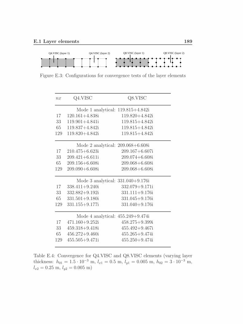
E.1 Layer elements 189
Q4.VISC (layer 1) Q4.VISC (layer 2) Q8.VISC (layer 1) Q8.VISC (layer 2)
Figure E.3: Configurations for convergence tests of the layer elements
nx Q4.VISC Q8.VISC
Mode 1 analytical: 119.815+4.842i17 120.161+4.838i 119.820+4.842i33 119.901+4.841i 119.815+4.842i65 119.837+4.842i 119.815+4.842i129 119.820+4.842i 119.815+4.842i
Mode 2 analytical: 209.068+6.608i17 210.475+6.623i 209.167+6.607i33 209.421+6.611i 209.074+6.608i65 209.156+6.608i 209.068+6.608i129 209.090+6.608i 209.068+6.608i
Mode 3 analytical: 331.040+9.176i17 338.411+9.240i 332.079+9.171i33 332.882+9.192i 331.111+9.176i65 331.501+9.180i 331.045+9.176i129 331.155+9.177i 331.040+9.176i
Mode 4 analytical: 455.249+9.474i17 471.160+9.252i 458.275+9.399i33 459.318+9.418i 455.492+9.467i65 456.272+9.460i 455.265+9.474i129 455.505+9.471i 455.250+9.474i
Table E.4: Convergence for Q4.VISC and Q8.VISC elements (varying layerthickness: h01 = 1.5 · 10−3 m, lx1 = 0.5 m, ly1 = 0.005 m, h02 = 3 · 10−3 m,lx2 = 0.25 m, ly2 = 0.005 m)

190 Convergence tests
Q4.VISC
HE8.ACOU HE20.ACOU
Q8.VISC
Figure E.4: Configurations for convergence tests of the layer elements
nx HE8.ACOU/Q4.VISC HE20.ACOU/Q8.VISC
Mode 1 analytical 1D: 104.915+0.911i17 105.143+0.916i 104.915+0.911i33 104.969+0.912i 104.910+0.910i65 104.923+0.910i 104.906+0.910i129 104.906+0.910i 104.897+0.909i
Mode 2 analytical 1D : 233.158+1.077i17 235.248+1.112i 233.318+1.082i33 233.676+1.087i 233.156+1.079i65 233.272+1.081i 233.134+1.079i129 233.156+1.081i 233.110+1.081i
Mode 3 analytical 1D : 337.734+2.320i17 343.369+2.384i 338.388+2.348i33 339.091+2.336i 337.694+2.320i65 337.964+2.322i 337.564+2.317i129 337.582+2.317i 337.401+2.314i
Mode 4 analytical 1D : 444.182+1.611i17 460.199+1.706i 447.267+1.616i33 448.181+1.631i 444.396+1.609i65 445.158+1.612i 444.160+1.605i129 444.381+1.604i 444.112+1.599i
Table E.5: Convergence for Q4.VISC/HE8.ACOU andQ8.VISC/HE20.ACOU elements (lx1 = 0.5 m, ly1 = 0.005 m,lz1 = 0.005 m,h02 = 3 · 10−3 m, lx2 = 0.25 m, ly2 = 0.005 m)

E.1 Layer elements 191
E.1.3 Acousto-elasticity
Consider a rectangular simply supported plate backed by a thin gas layer.The behaviour of the plate is decribed using the Kirchhoff equation:
Ept3p
12(1− ν2
p
) [∂4vp∂x4
+ 2∂2vp∂x2
∂2vp∂y2
+∂4vp∂y4
]+ ρptp
∂2vp∂t2
= p− p0 (E.1)
where vp is the velocity of the plate in the z-direction, Ep is Young’s modulus,ρp is the density and νp is Poisson’s ratio of the plate material. Introducingdimensionless quantities:
vp = c0vpeiωt ; p = p0
[1 + peiωt
]x =
ωx
c0
; y =ωy
c0
(E.2)
The pressure distribution in the layer is described with the low reduced fre-quency model. The acousto-elastic behaviour of the system is described bythe following set of equations:
k4
[∂4vp∂x4
+ 2∂2vp∂x2
∂2vp∂y2
+∂4vp∂y4
]− Ω2k4
k4x
vp = iΩ2εk3
γk4x
p
k2
[∂2p
∂x2+∂2p
∂y2
]− k2Γ2p = −1
2ikn (sσ) vp (E.3)
For a simply supported panel, the mode shapes are:
vp = Bqr sin(qπ
2
[x
lx+ 1
])sin
(rπ
2
[y
ly+ 1
])q = 1, 2, · · · r = 1, 2, · · ·
p = Cqr sin(qπ
2
[x
lx+ 1
])sin
(rπ
2
[y
ly+ 1
])(E.4)
Inserting these expressions finally gives the following set of equations:[A11 A12
A21 A22
]Bqr
Cqr
=
00
(E.5)
where the matrix elements are given by:
A11 = −iΩ2εk3
γk4x
A12 = k4
[(qπ
2kx
)4
+ 2(qπ
2kx
)2 ( rπ
2akx
)2
+(rπ
2akx
)4]− Ω2k4
k4x
A21 = k2
[−(qπ
2kx
)2
−(rπ
2akx
)2]− k2Γ2 (E.6)
A22 =1
2iknΓ2

192 Convergence tests
The structural modes, the acoustic modes and the acousto-elastic modes areobtained from:
structural modes : A11 = 0
acoustic modes : A22 = 0 (E.7)
acousto− elastic modes : A11A22 − A21A12 = 0
The eigenfrequencies were solved with a simple minimization procedure inMatlab, setting the absolute value equal to zero. This proved to be a fastand stable approach. The results are given in Tables E.6, E.7 and E.8
nx ny Q4.VISC
Mode 11 analytical: 468.990+12.070i9 9 472.047+12.108i17 17 469.753+12.079i20 20 469.479+12.076i33 33 469.181+12.072i
Mode 21 analytical: 745.366+15.119i9 9 761.933+15.282i17 17 749.487+15.160i20 20 748.002+15.145i33 33 746.395+15.129i
Mode 22 analytical: 944.909+16.977i9 9 969.562+17.192i17 17 951.046+17.030i20 20 948.835+17.011i33 33 946.442+16.990i
Table E.6: Convergence for Q4.VISC elements. (h0 = 1.5 · 10−3 m, lx =0.25 m, ly = 0.25 m)

E.1 Layer elements 193
nx ny Q4.VISC
Mode 11 analytical: 19.3269 9 19.64017 17 19.40320 20 19.37533 33 19.344
Mode 21 analytical: 48.3179 9 51.40517 17 49.05420 20 48.78533 33 48.496
Mode 22 analytical: 77.3079 9 82.50617 17 78.55620 20 78.10033 33 77.609
Table E.7: Convergence for Q4.ST elements. (lx = 0.25 m, ly = 0.25 m,Ep = 70 · 109 N/m2, ρp = 2710 kg/m3, νp = 0.3, tp = 1 · 10−3 m)

194 Convergence tests
nx ny Q4.VISC
Mode 11 analytical: 10.711+1.094i9 9 10.937+1.096i17 17 10.766+1.094i20 20 10.746+1.094i
Mode 21 analytical: 35.604+1.150i9 9 38.285+1.157i17 17 36.244+1.152i20 20 36.011+1.151i
Mode 22 analytical: 62.851+1.096i9 9 67.679+1.093i17 17 64.101+1.095i20 20 63.588+1.095i
Table E.8: Convergence for Q4.VIS, INT.8 and Q4.ST elements. (h0 =1.5 · 10−3 m, lx = 0.25 m, ly = 0.25 m, Ep = 70 · 109 N/m2, ρp = 2710 kg/m3,νp = 0.3, tp = 1 · 10−3 m)
E.2 Tube elements 195
E.2 Tube elements
E.2.1 Eigenfrequency calculations
Eigenfrequency calculations were carried out for various configurations. Inall cases both ends of the (composed) tube were terminated by a p = 0 con-dition. The results for a line of T2.VISC elements and a line of T3.VISCelements are given in Table E.9 and Table E.10. The results for a line, com-posed of two different segments of T2.VISC elements or T3.VISC elementswith different cross-sectional areas are given in Tables E.11, E.12 and E.13.Finally, the viscothermal tube elements were coupled to standard acousticvolume elements. The results for these calculations are given in Table E.14and Table E.15
The analytical solution can easily be obtained for these 1-dimensionalproblems and will not be discussed in detail here. In the case of differentsegments, continuity of pressure and conservation of mass on the interfaceis assumed. Please note that in the test cases with the standard acousticvolume elements, the solution does not have to converge fully to the analyt-ical solution, since the finite elements are based on a 3-dimensional volumeapproach. For a small cross section of the tube, however, the differences aresmall.
The Tables show good agreement between the analytical and numericalresults. It can be concluded that the viscothermal elements give good results.Furthermore, viscothermal elements with different cross sections can easilybe coupled. Finally, the viscothermal elements can be coupled to standardacoustic volume elements.

196 Convergence tests
T2.VISC T3.VISC
Figure E.5: Configurations for convergence tests of the tube elements
nx T2.VISC T3.VISC
Mode 1 analytical: 155.947+14.126i17 156.208+14.138i 155.950+14.127i33 156.012+14.129i 155.947+14.126i65 155.963+14.127i 155.947+14.126i129 155.951+14.127i 155.947+14.126i
Mode 2 analytical: 320.095+19.953i17 322.219+20.017i 320.180+19.956i33 320.625+19.969i 320.101+19.953i65 320.227+19.957i 320.096+19.953i129 320.128+19.954i 320.095+19.953i
Mode 3 analytical: 485.609+24.428i17 492.834+ 24.604i 486.231+24.443i33 487.410+ 24.472i 485.650+24.429i65 486.059+ 24.439i 485.612+24.428i129 485.722+ 24.431i 485.610+24.428i
Mode 4 analytical: 651.829+28.202i17 669.051+28.564i 654.329+28.255i33 656.115+28.292i 652.000+28.206i65 652.899+28.225i 651.840+28.202i129 652.096+28.208i 651.830+28.202i
Table E.9: Convergence for T2.VISC and T3.VISC elements (circular crosssection: R = 1.5 · 10−3 m, lx = 0.5 m)

E.2 Tube elements 197
T2.VISC T3.VISC
Figure E.6: Configurations for convergence tests of the tube elements
nx T2.VISC T3.VISC
Mode 1 analytical: 157.689+12.190i17 157.952+12.200i 157.692+12.190i33 157.754+12.192i 157.689+12.190i65 157.705+12.190i 157.689+12.190i129 157.693+12.190i 157.689+12.190i
Mode 2 analytical: 322.573+17.292i17 324.706+17.348i 322.658+17.294i33 323.105+17.306i 322.579+17.292i65 322.706+17.296i 322.574+17.292i129 322.606+17.293i 322.574+17.292i
Mode 3 analytical: 488.650+21.209i17 495.897+21.364i 489.274+21.223i33 490.457+21.248i 488.691+21.210i65 489.101+21.219i 488.653+21.209i129 488.763+21.212i 488.651+21.209i
Mode 4 analytical: 655.343+24.512i17 672.610+24.829i 657.850+24.559i33 659.641+24.592i 655.515+24.516i65 656.416+24.532i 655.355+24.513i129 655.611+24.517i 655.344+24.512i
Table E.10: Convergence for T2.VISC and T3.VISC elements (rectangularcross section: lx = 0.5 m, ly = 1.5 · 10−3 m, lz = 2 · 10−3 m)

198 Convergence tests
T2.VISC (area 1) T2.VISC (area 2) T3.VISC (area 2)T3.VISC (area 1)
Figure E.7: Configurations for convergence tests of the tube elements
nx T2.VISC T3.VISC
Mode 1 analytical: 125.677+9.722i17 126.104+9.703i 125.685+9.721i33 125.784+9.717i 125.678+9.722i65 125.704+9.720i 125.678+9.722i129 125.684+9.721i 125.677+9.722i
Mode 2 analytical: 192.606+12.081i17 193.722+12.132i 192.677+12.082i33 192.886+12.093i 192.611+12.081i65 192.676+12.084i 192.606+12.081i129 192.624+12.081i 192.606+12.081i
Mode 3 analytical: 321.198+18.892i17 329.056+19.076i 322.331+18.902i33 323.158+18.938i 321.275+18.893i65 321.688+18.903i 321.203+18.892i129 321.321+18.895i 321.198+18.892i
Mode 4 analytical: 457.004+18.900i17 473.486+17.859i 460.360+18.527i33 461.316+18.637i 457.281+18.868i65 458.094+18.834i 457.023+18.898i129 457.278+18.883i 457.006+18.900i
Table E.11: Convergence for T2.VISC and T3.VISC elements (circular crosssections: R1 = 1.5 · 10−3 m, lx1 = 0.5 m, R2 = 3 · 10−3 m, lx2 = 0.25 m)

E.2 Tube elements 199
T2.VISC (area 1) T2.VISC (area 2) T3.VISC (area 2)T3.VISC (area 1)
Figure E.8: Configurations for convergence tests of the tube elements
nx T2.VISC T3.VISC
Mode 1 analytical: 126.851+8.375i17 127.275+8.360i 126.858+8.375i33 126.957+8.372i 126.851+8.375i65 126.877+8.374i 126.851+8.375i129 126.857+8.375i 126.851+8.375i
Mode 2 analytical: 194.131+10.476i17 195.253+10.522i 194.202+10.478i33 194.412+10.488i 194.135+10.477i65 194.201+10.480i 194.131+10.477i129 194.148+10.477i 194.131+10.477i
Mode 3 analytical: 323.539+16.371i17 331.419+16.533i 324.673+16.381i33 325.505+16.412i 323.617+16.373i65 324.030+16.382i 323.544+16.372i129 323.662+16.374i 323.540+16.372i
Mode 4 analytical: 459.263+16.341i17 475.618+15.456i 462.575+16.028i33 463.541+16.120i 459.536+16.319i65 460.344+16.289i 459.281+16.344i129 459.534+16.331i 459.264+16.345i
Table E.12: Convergence for T2.VISC and T3.VISC elements (rectangularcross sections: lx1 = 0.5 m, ly1 = 1.5 · 10−3 m, lz1 = 2 · 10−3 m, lx2 = 0.25 m,ly2 = 3 · 10−3 m, lz2 = 4 · 10−3 m)

200 Convergence tests
T2.VISC (area 1) T2.VISC (area 2) T3.VISC (area 2)T3.VISC (area 1)
Figure E.9: Configurations for convergence tests of the tube elements
nx T2.VISC T3.VISC
Mode 1 analytical: 133.032+9.686i17 133.523+9.650i 133.042+9.684i33 133.155+9.677i 133.033+9.686i65 133.063+9.684i 133.032+9.686i129 133.040+9.685i 133.032+9.686i
Mode 2 analytical: 186.311+11.015i17 187.275+11.088i 186.367+11.018i33 186.553+11.034i 186.315+11.016i65 186.372+11.020i 186.311+11.016i129 186.326+11.017i 186.311+11.016i
Mode 3 analytical: 320.860+19.218i17 328.983+19.426i 322.036+19.237i33 322.885+19.270i 320.940+19.220i65 321.366+19.231i 320.865+19.219i129 320.986+19.222i 320.860+19.218i
Mode 4 analytical: 464.901+18.728i17 481.973+16.825i 468.645+18.051i33 469.474+18.258i 465.213+18.677i65 466.062+18.615i 464.921+18.728i129 465.192+18.702i 464.902+18.731i
Table E.13: Convergence for T2.VISC and T3.VISC elements (circular andrectangular cross sections: R = 1.5 · 10−3 m, lx1 = 0.5 m, lx2 = 0.25 m,ly2 = 3 · 10−3 m, lz2 = 4 · 10−3 m)

E.2 Tube elements 201
HE8.ACOU
T2.VISC T3.VISC
HE20.ACOU
Figure E.10: Configurations for convergence tests of the tube elements
nx HE8.ACOU/T2.VISC HE20.ACOU/T3.VISC
Mode 1 analytical 1D: 95.877+1.145i17 96.060+1.150i 95.876+1.144i33 95.920+1.146i 95.872+1.144i65 95.881+1.144i 95.866+1.143i129 95.866+1.142i 95.855+1.140i
Mode 2 analytical 1D: 241.578+1.533i17 244.142+1.616i 241.779+1.544i33 242.210+1.556i 241.570+1.538i65 241.712+1.544i 241.536+1.542i129 241.564+1.545i 241.493+1.550i
Mode 3 analytical 1D: 333.617+6.465i17 337.944+6.552i 333.959+6.504i33 334.574+6.484i 333.425+6.457i65 333.608+6.458i 333.177+6.444i129 333.134+6.440i 332.759+6.424i
Mode 4 analytical 1D: 434.907+1.962i17 451.333+2.007i 438.203+1.941i33 438.990+1.965i 435.127+1.954i65 435.902+1.953i 434.879+1.945i129 435.109+1.941i 434.824+1.929i
Table E.14: Convergence for HE8.ACOU/T2.VISC andHE20.ACOU/T3.VISC elements (rectangular and circular cross sec-tions: lx1 = 0.5 m, ly1 = 2.5 · 10−3 m, lz1 = 2.5 · 10−3 m, ny1 = 3, nz1 = 3(HE8.AOU), ny1 = 5, nz1 = 5 (HE20.ACOU), R2 = 3 ·10−3 m, lx2 = 0.25 m)

202 Convergence tests
HE8.ACOU
T2.VISC T3.VISC
HE20.ACOU
Figure E.11: Configurations for convergence tests of the tube elements
nx HE8.ACOU/T2.VISC HE20.ACOU/T3.VISC
Mode 1 analytical 1D: 101.489+1.386i17 101.697+1.393i 101.485+1.385i33 101.534+1.386i 101.477+1.384i65 101.486+1.384i 101.464+1.381i129 101.461+1.380i 101.439+1.377i
Mode 2 analytical 1D: 235.483+1.719i17 237.689+1.786i 235.641+1.730i33 236.015+1.739i 235.454+1.726i65 235.570+1.731i 235.402+1.731i129 235.416+1.735i 235.324+1.742i
Mode 3 analytical 1D: 335.544+4.516i17 340.692+4.618i 335.998+4.560i33 336.661+4.540i 335.280+4.511i65 335.483+4.512i 334.941+4.498i129 334.870+4.495i 334.369+4.479i
Mode 4 analytical 1D: 440.339+2.429i17 456.434+2.545i 443.471+2.424i33 444.335+2.449i 440.525+2.418i65 441.283+2.419i 440.258+2.402i129 440.470+2.396i 440.153+2.374i
Table E.15: Convergence for HE8.ACOU/T2.VISC andHE20.ACOU/T3.VISC elements (rectangular cross sections: lx1 = 0.5 m,ly1 = 0.0025 m, lz1 = 0.0025 m, ny1 = 3, ny1 = 3 (HE8.ACOU), nz1 = 5,nz1 = 5 (HE20.ACOU), ly2 = 3 · 10−3 m, lz2 = 4 · 10−3 m, lx2 = 0.25 m)