
Viscoelastic finite element modeling of deformation ... · Viscoelastic finite element modeling of...
172
Viscoelastic finite element modeling of deformation transients of single cells Soo Kng Teo A thesis submitted to Imperial College London for the degree of Doctor of Philosophy Imperial College London Department of Bioengineering 2008
Transcript of Viscoelastic finite element modeling of deformation ... · Viscoelastic finite element modeling of...
Viscoelastic finite element modeling of
deformation transients of single cells
Soo Kng Teo
A thesis submitted to Imperial College London
for the degree of Doctor of Philosophy
Imperial College London
Department of Bioengineering
2008
Viscoelastic finite element modeling of deformation transients of single cells
2
Abstract
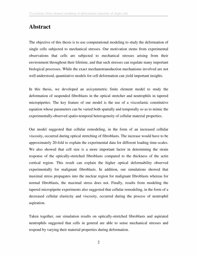
The objective of this thesis is to use computational modeling to study the deformation of
single cells subjected to mechanical stresses. Our motivation stems from experimental
observations that cells are subjected to mechanical stresses arising from their
environment throughout their lifetime, and that such stresses can regulate many important
biological processes. While the exact mechanotransduction mechanisms involved are not
well understood, quantitative models for cell deformation can yield important insights.
In this thesis, we developed an axisymmetric finite element model to study the
deformation of suspended fibroblasts in the optical stretcher and neutrophils in tapered
micropipettes. The key feature of our model is the use of a viscoelastic constitutive
equation whose parameters can be varied both spatially and temporally so as to mimic the
experimentally-observed spatio-temporal heterogeneity of cellular material properties.
Our model suggested that cellular remodeling, in the form of an increased cellular
viscosity, occurred during optical stretching of fibroblasts. The increase would have to be
approximately 20-fold to explain the experimental data for different loading time-scales.
We also showed that cell size is a more important factor in determining the strain
response of the optically-stretched fibroblasts compared to the thickness of the actin
cortical region. This result can explain the higher optical deformability observed
experimentally for malignant fibroblasts. In addition, our simulations showed that
maximal stress propagates into the nuclear region for malignant fibroblasts whereas for
normal fibroblasts, the maximal stress does not. Finally, results from modeling the
tapered micropipette experiments also suggested that cellular remodeling, in the form of a
decreased cellular elasticity and viscosity, occurred during the process of neutrophil
aspiration.
Taken together, our simulation results on optically-stretched fibroblasts and aspirated
neutrophils suggested that cells in general are able to sense mechanical stresses and
respond by varying their material properties during deformation.

Viscoelastic finite element modeling of deformation transients of single cells
3
Acknowledgement
I have been very fortunate to be given this chance to purse a doctorate degree, one of my
many dreams and a route less well traveled among my friends. There are a lot of people
whom I want to thank, for their help, support and encouragement during the past 4 years
of my life as I struggle along this long and demanding path.
First and foremost, I would like to thank my supervisor, Professor Kim Parker, for his
patience, encouragement and guidance during the course of this research work. I am
grateful for all the knowledge that you had shared with me and I have definitely learnt a
lot from you. I would also like to thank my co-supervisor, Dr. Chiam Keng Hwee, who
taught me how to think independently. Special thanks also go to my ex-supervisor, Dr.
Andrew Goryachev. I would have never started on this research project without him.
I would also like to express my gratitude to my ex-colleagues in the Bioinformatics
Institute and my current colleagues in the biophysics team in the Institute of High
Performance Computing. All of you helped to create an environment conducive for
research, where I do not have to worry about any administrative or logistics issues.
I gratefully acknowledge the financial support from the Agency of Science, Technology
and Research. Many thanks to my scholarship officers, Serene, Swee Bee, Joanne, Cindy
and others for their support with all the administrative matters as well as my fellow
friends on the same scholarship program: Kwang Hwee, Sing Yang, Zi En and Ho Huat,
for all the suffering and enjoyment we all shared along this journey.
Friends have always been a very important part of my life especially during times where
the going gets tough. For that, I have to thank Dave, James, Seath, Han Hui and Phey
Leng. You kept me sane during those times when my research was going nowhere and
the problems that I faced seem insurmountable.

Viscoelastic finite element modeling of deformation transients of single cells
4
Lastly, I want to thank my mum for being there for me throughout all my life. Her
patience and support has been my pillar of strength. Without her, I would never have the
courage to dream.
Viscoelastic finite element modeling of deformation transients of single cells
5
Table of Content
Abstract.............................................................................................................................. 2
Acknowledgement ............................................................................................................. 3
Table of Content................................................................................................................ 5
List of Figures.................................................................................................................... 9
List of Tables ................................................................................................................... 16
Chapter 1. Introduction............................................................................................. 18
Chapter 2. Literature review .................................................................................... 22
2.1 Structure of an eukaryotic cell ............................................................................ 23
2.1.1 Cytoskeleton ..................................................................................................... 25
2.2 Experimental Techniques..................................................................................... 27
2.2.1 Localized perturbations ................................................................................... 28
2.2.1.1 Atomic force microscopy........................................................................... 28
2.2.1.2 Magnetic twisting cytometry ..................................................................... 29
2.2.1.3 Cytoindentation......................................................................................... 30
2.2.2 Entire cell perturbations .................................................................................. 31
2.2.2.1 Laser/optical tweezers .............................................................................. 31
2.2.2.2 Microplate stretcher.................................................................................. 32
2.2.2.3 Microfabricated post array detector......................................................... 32
2.2.2.4 Micropipette aspiration ............................................................................ 33
2.2.2.5 Shear flow ................................................................................................. 34
2.2.2.6 Substrate stretcher .................................................................................... 34
2.2.2.7 Optical stretcher ....................................................................................... 35
2.3 Overview of Mechanical Models ......................................................................... 36
2.3.1 Micro/Nanostructural Approach ..................................................................... 37
2.3.1.1 Open-cell foam model ............................................................................... 38
2.3.1.2 Stress-supported structures....................................................................... 39
2.3.1.3 Tensegrity architecture ............................................................................. 40
2.3.2 Continuum approach........................................................................................ 41
2.3.2.1 Cortical shell-liquid core models.............................................................. 41
Viscoelastic finite element modeling of deformation transients of single cells
6
2.3.2.1.1 Newtonian liquid drop model ............................................................ 42
2.3.2.1.2 Compound Newtonian liquid drop model.......................................... 42
2.3.2.1.3 Shear thinning liquid drop................................................................. 43
2.3.2.1.4 Maxwell liquid drop model ................................................................ 44
2.3.2.2 Solid models .............................................................................................. 44
2.3.2.2.1 Linear elastic solid model.................................................................. 44
2.3.2.2.2 Viscoelastic solid model..................................................................... 45
2.3.2.2.3 Power-law dependent model.............................................................. 46
Chapter 3. Numerical method................................................................................... 47
3.1 Linear finite element scheme ............................................................................... 48
3.1.1 Preliminary ...................................................................................................... 48
3.1.2 Linear elastic constitutive equations ............................................................... 49
3.1.3 Finite element discretization............................................................................ 51
3.1.4 Formulation of the consistent mass matrix and damping matrix .................... 52
3.1.5 Numerical solution techniques......................................................................... 54
3.2 Viscoelastic finite element formulation using the generalized Maxwell model.
...................................................................................................................................... 58
3.2.1 Constitutive equation of the generalized Maxwell model (one dimension). .... 59
3.2.2 Constitutive equation of the generalized Maxwell model for multi-axial stress
states ......................................................................................................................... 60
3.2.3 Finite element formulation............................................................................... 61
3.2.4 Non-dimensionalization ................................................................................... 62
3.2.5 Test results ....................................................................................................... 65
3.2.5.1 Description of the benchmark problem..................................................... 65
3.2.5.2 Simulation Results..................................................................................... 66
3.2.5.3 Effects of inertia on the dynamic response ............................................... 73
3.3 Viscoelastic finite element formulation using the 3 parameter fluid model .... 75
3.3.1 Constitutive equation of the 3 parameter fluid model (one dimension)........... 75
3.3.2 Constitutive equation of the 3 parameter fluid model for multi-axial stress
states ......................................................................................................................... 77
3.4 Viscoelastic finite element formulation using the Kelvin-Voigt model ............ 79
Viscoelastic finite element modeling of deformation transients of single cells
7
3.4.1 Constitutive equation of the Kelvin-Voigt model (one dimension) .................. 79
3.4.2 Constitutive equation of the Kelvin-Voigt model for multi-axial stress states
............................................................................................................................... 83
3.5 Axisymmetric stress analysis ............................................................................... 84
3.5.1 Linear elastic constitutive equations ............................................................... 85
3.5.2 Finite element formulation............................................................................... 88
Chapter 4. Single cell deformation in the optical stretcher.................................... 91
4.1 Introduction........................................................................................................... 91
4.2 Finite-element formulation .................................................................................. 93
4.2.1 Model parameters ............................................................................................ 94
4.3 Results .................................................................................................................. 103
4.3.1 Cellular remodeling of optically stretched fibroblast cells is necessary to fit
experimental data.................................................................................................... 103
4.3.2. Maximal strain developed depends on size of suspended fibroblast cells being
stretched .................................................................................................................. 110
4.3.3. Extent of intracellular stress propagation depends on size of suspended
fibroblast cells being stretched ............................................................................... 115
4.4. Conclusion .......................................................................................................... 119
Chapter 5. Single cell deformation in the tapered micropipette.......................... 121
5.1 Introduction......................................................................................................... 121
5.2 The tapered micropipette experiment............................................................... 123
5.3 Finite-element formulation ................................................................................ 126
5.3.1 Model parameters .......................................................................................... 126
5.3.2 Model Geometry............................................................................................. 128
5.3.3 Contact Heuristics ......................................................................................... 129
5.4 Results .................................................................................................................. 132
5.4.1 Temporal variation of neutrophil rheological properties provides better fit to
experimental data.................................................................................................... 132
5.5. Conclusion .......................................................................................................... 142
Chapter 6. Conclusion and future work ................................................................ 144
References...................................................................................................................... 147

Viscoelastic finite element modeling of deformation transients of single cells
8
Appendix 1: Analytical solution for the deformation of a solid, homogeneous elastic
sphere ............................................................................................................................. 164
Viscoelastic finite element modeling of deformation transients of single cells
9
List of Figures
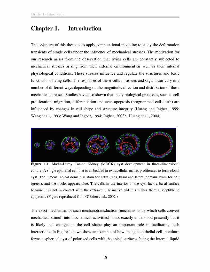
Figure 1.1: Madin-Darby Canine Kidney (MDCK) cyst development in three-
dimensional culture. A single epithelial cell that is embedded in extracellular matrix
proliferates to form clonal cyst. The lumenal apical domain is stain for actin (red), basal
and lateral domain strain for p58 (green), and the nuclei appears blue. The cells in the
interior of the cyst lack a basal surface because it is not in contact with the extra-cellular
matrix and this makes them susceptible to apoptosis. (Figure reproduced from O’Brien et
al., 2002.) .......................................................................................................................... 18
Figure 2.1: Diagram showing the typical structure of a eukaryotic cell. (Figure
reproduced from Alberts et al., 2002.).............................................................................. 24
Figure 2.2: Schematic illustration of the different experimental techniques used to probe
mechanical compliance of cells. (Figure reproduced from Suresh, 2007.) ...................... 28
Figure 2.3: Schematic of the stretching of a cell trapped in the optical stretcher. The cell
is stably trapped in the middle by the optical forces from the two laser beams. (Figure
reproduced from Guck et al., 2001.) ................................................................................. 35
Figure 2.4: Overview of common mechanical models used for modeling cellular
response of living cells. (Figure reproduced from Lim et al., 2006.) ............................... 37
Figure 2.5: Schematic of the open-cell foam model. (a) Unit cell representation of the
cytoskeletion. (b) Loading of unit cell due to shear stress, indicating mechanism of
deformation due to transmitted force, F. (Figure reproduced from Satcher and Dewey,
1996.) ................................................................................................................................ 39
Figure 2.6: Schematic of the tensegrity model. The structure contains a series of isolated
compression-resistant elements (white struts) that resist the pull of surrounding tensile
elements (black cables) and impose a prestress that stabilizes the entire network. (Figure
reproduced from Ingber, 1997.) ........................................................................................ 40
Figure 2.7: Different variations of the cortical shell-liquid core models (continuum
approach). (Figure adapted from Lim et al., 2006.).......................................................... 43
Figure 3.1: Finite element discretization of a two dimensional solid represented by a
circle of unit radius in non-dimensional units................................................................... 51
Viscoelastic finite element modeling of deformation transients of single cells
10
Figure 3.2: Shape function for a linear triangle element. The displacement x
u and yu at
an arbitrary point 1 2 3( , , )P ξ ξ ξ is computed from the known nodal displacements at the
vertices of the linear triangle............................................................................................. 51
Figure 3.3: Initial configuration of a solid body at time-step n represented by the
configuration n
p and the deformed configuration at time-step n+1 represented by the
configuration 1n+p . ............................................................................................................ 57
Figure 3.4: Representation of a generalized Maxwell (G-M) model. It consists of a single
spring element (µ0) in parallel connection with n Maxwell models. Each Maxwell model
consists of one spring element (µi) in series connection to a dashpot element (ηi). ......... 59
Figure 3.5: Geometry used in our benchmark problem simulation for the uniaxial
stretching of a rectangular block. Making use of the symmetric nature of the problem, we
are required only to model one-quarter of the block. Sliding boundary conditions are
prescribed for nodal points lying on both the x- and y- axis to reflect the symmetrical
boundary conditions.......................................................................................................... 65
Figure 3.6: Finite element discretization of the problem domain with description of the
imposed boundary conditions. .......................................................................................... 66
Figure 3.7: Comparison of simulation results with the analytical solution for the
benchmark problem for loading phase only. The values of the simulation parameters are
summarized in Table 3.1. We can see that the 1D simulation results coincide exactly with
the analytical solution. However, our finite element simulation results seem to differ
rather significantly. ........................................................................................................... 67
Figure 3.8: Effects of the time-step size on our finite element simulation results. We
varied the size of the time-step ( t∆ ) used in our simulation while keeping the values of
the other parameters constant. The results obtained from our simulation are compared
with the analytical solution. (a) Strain response for 0 80t≤ ≤ . (b) Magnified view of the
strain response for 50 80t≤ ≤ . We can see that the error between our finite element
simulation and the analytical solution is not sensitive to the size of the time-step used in
the simulation.................................................................................................................... 69
Figure 3.9: Comparison of simulation results with the analytical solution for the
benchmark problem after correction. Taking into account of the changes in the cross-
Viscoelastic finite element modeling of deformation transients of single cells
11
sectional area and loading for the finite element simulation, we can see that the corrected
results are in excellent agreement with the analytical solution......................................... 72
Figure 3.10: Effects of inertia on the dynamic response of our finite element simulation.
For the case of 41*10ρ −=% , we can see that there is a very slight oscillatory response in
the system that corresponds to the effects of inertia. When the dimensionless density ρ~ is
reduced further, the oscillatory response becomes almost non-evident. .......................... 74
Figure 3.11: Representation of a 3 parameter fluid (3pF) model. It consists of a linear
dashpot connected in series with a Kelvin-Voigt (K-V) element, which is a linear spring
connected in parallel with a linear dashpot....................................................................... 75
Figure 3.12: Representation of a standard linear solid (SLS) model. It consists of a single
spring element (µ0) in parallel connection with a Maxwell model. The Maxwell model
consists of another spring element (µ1) in series connection to a dashpot element (η1). .. 78
Figure 3.13: Representation of the three-parameter fluid model using two standard linear
solids arranged in series. The value of the single spring element (µ01) in the first SLS is
set to approaching zero while the values of the spring elements in the Maxwell model (µ11
and µ12) for both SLS are set to approaching infinity. These have the effect of “short-
circuiting” the contributions of these spring elements to the response of the two SLS in
series, thereby allowing us to mimic the response of the three-parameter fluid model.... 78
Figure 3.14: Representation of a Kelvin-Voigt (K-V) model. It consists of a spring
element ( E ) in parallel connection with a dashpot element (η )...................................... 79
Figure 3.15: Analytical strain response for the one-dimensional Kelvin-Voigt (K-V)
model under a constant stress applied as a step load at time 0t = . We note that the K-V
model exhibits no instantaneous strain response at time 0t+= and the strain approaches
an asymptotic value ( )0 / Eσ as t → ∞ ............................................................................ 81
Figure 3.16: Representation of the Kelvin-Voigt (K-V) model using the standard linear
solid (SLS). The value of the single spring element (µ1) in the Maxwell element of the
SLS is set to approaching infinity which has the effect of “short-circuiting” the
contribution of this spring element to the response of the SLS. This approach allows us to
mimic the response of the K-V model. ............................................................................. 83
Viscoelastic finite element modeling of deformation transients of single cells
12
Figure 3.17: Element of an axisymmetric solid (Figure reproduced from Zienkiewicz and
Taylor, 1989)..................................................................................................................... 85
Figure 3.18: Strains and stresses involved in the analysis of axisymmetric solids (Figure
reproduced from Zienkiewicz and Taylor, 1989). ............................................................ 86
Figure 4.1: (a) Schematic of the two-dimensional geometry of a cell of radius unity and
definition of the parameter ρ used in our finite-element simulation. (b) Spatial variation
of the material properties of the 3 parameter fluid model with the radial coordinate ρ. The
elasticity k of the cell decreases exponentially away from the cortical region while the
viscosities exhibit the opposite trend. 2η varies in a similar manner as 1η with respect to
ρ......................................................................................................................................... 94
Figure 4.2: Fluorescence confocal images of the actin cytoskeleton (red) in suspended
fibroblasts. (a) Normal. (b) Malignant. We can see that the actin filaments are highly
localized in the cortical region of the suspended fibroblasts (Figure reproduced from
Guck et al., 2005).............................................................................................................. 98
Figure 4.3: Sensitivity analysis to determine if our simulation results (the strain response
along the long axis of the cell) are dependent on the values of the parameter α . (a) We
observe that our results are dependent on the value of α chosen and the strain response
curve obtained using a value of α =2.5 gives us the best fit to the experimental data (b)-
(c) Variation of the material properties, elasticity ( k ) and viscosity ( 1η ) with the radial
coordinate (p) for different values of α . ........................................................................ 101
Figure 4.4: Sensitivity analysis to determine if our simulation results (the strain response
along the long axis of the cell) are dependent on the functional form of the spatial
variation. (a) The strain response obtained from using the exponential variation gives the
best fit to the experimental data as compared to the linear and logarithm variation (b)-(c)
Variation of the material properties, elasticity ( k ) and viscosity ( 1η ) with the radial
coordinate (p) for the different functional form of spatial variation............................... 102
Figure 4.5: Schematic of the optical stretching of a suspended cell. The stretching force
is generated on the surface of the cell and acts normal to the cell surface. This stretching
force can be approximated by the analytical function 0 cosnσ σ θ= where n is a
Viscoelastic finite element modeling of deformation transients of single cells
13
parameter that is dependent on the experimental setup and the size of the cell. (Figure
adapted from Guck et al., 2001.)..................................................................................... 103
Figure 4.6: Fitting of the experimental strain development when subjected to 0.2 s
loading (crosses) and 2.5 s loading (circles) with a single set of spatiotemporally-varying
parameters as described in Equations (80-83) and (85) that is supposed to mimic cellular
remodeling. The good fits to both data sets suggest that cellular remodeling has occurred
during optical stretching. ................................................................................................ 108
Figure 4.7: The strain along the laser axis, denoted by r
ε (blue solid line), for a solid
homogeneous elastic sphere subjected to a surface stress profile as given in Equation (84)
computed using our finite element model. We can see that r
ε is sensitively dependent on
the parameter n in Equation (84). For larger values of n (corresponding to a more
localised stretching profile), r
ε is smaller compared to the case of a smaller value of n
(corresponding to a broad stretching profile).................................................................. 114
Figure 4.8: Strain for a suspended fibroblast obtained using our viscoelastic finite
element deformation. We investigated the effects of varying either the cortical thickness
or the surface stretching profile (represented by the parameter n in Equation (84)) on the
strain (r
ε ). First, cortical thickness was varied from 10% to 25% (blue: 10%, red: 15%,
green: 20% and black: 25%) while keeping all other parameters constant. Next, the
parameter n was varied from 4 to 24. The strain (r
ε ) is more sensitive to the variation in
the parameter n than variation in the cortical thickness and is smaller for larger values of
n compared to those case smaller values of n. This supports the experimental observation
that cancerous cells deform more compared to their normal counterparts. .................... 115
Figure 4.9: Von Mises stress distribution within the interior of the fibroblast at 2.5 s
obtained from finite element simulation: (a) normal fibroblasts subjected to a localized
surface stretching (n=24), (b) malignant fibroblasts subjected to a broad surface
stretching (n=4). For the localized stress distribution, we see that the regions with the
highest Von Mises stress concentration are offset from the centre of the cell and occur at
a region just beneath the cortical region. This observation is distinctly different from that
observed for the broad stress distribution in which the region of highest Von Mises stress
is in the perinuclear region of the cell............................................................................. 118
Viscoelastic finite element modeling of deformation transients of single cells
14
Figure 5.1: Videomicrograph of the tapered micropipette experimental measurements.
(a) ∆P = 0 dyn/cm2: a single passive cell was selected and aspirated into the tapered
pipette and allowed to recover to its resting spherical shape in the larger lumen of the
pipette. (b) ∆P = 25 dyn/cm2: a small positive pipette pressure was then applied and the
cell was very gently deformed into a bolus shape as it was driven down the pipette; it
then came to rest in the taper. (c) ∆P = 50 dyn/cm2 and (d) ∆P = 75 dyn/cm2: step
increases in pipette pressure then drove the cell to new equilibrium positions. (Figure
reproduced from Needham and Hochmuth, 1992.) ........................................................ 125
Figure 5.2: Neutrophil geometry used in our tapered micropipette simulation represented
by a semi-circle with non-dimensional radius of one unit. Making use of the
axisymmetric nature of the problem, we modeled only half the neutrophil along with the
upper boundary of the micropipette (represented by the thick solid line). Frictionless
sliding boundary conditions are prescribed for nodal points lying along (1) the horizontal
axis (r = 0) and (2) the boundary of the tapered micropipette. The driving pressure is
applied from the left-hand side of the cell as a Neumann type boundary condition. ..... 130
Figure 5.3: Enlarged view of the neutrophil geometry near the boundary of the pipette.
(a) Nodal points in contact with this inclined boundary (denoted by red circle) are
constrained to slide frictionlessly along this boundary through the application of the
Lagrange multiplier technique. The sliding boundary condition imposed prevents these
nodal points from penetrating through the boundary. (b) As the neutrophil deforms, nodal
points previously not in contact with the pipette boundary can penetrate through this
surface (denoted by green asterisk). To enforce non-penetration, we project these nodal
points back onto the pipette boundary at the end of the time-step. We also imposed a
sliding boundary condition along the inclined boundary for these nodal points for the
subsequent time-steps in the simulation. ........................................................................ 131
Figure 5.4: Driving pressure profile with respect to time used in our tapered micropipette
simulation. (a) ∆P = 25 dyn/cm2. The neutrophil is subjected to a constant driving
pressure over a time duration of 30 seconds and allowed to reach an equilibrium state. (b-
c) ∆P = 50 dyn/cm2 and ∆P = 75 dyn/cm2. The neutrophil is subjected to an initial driving
pressure of ∆P = 25 dyn/cm2 and allowed to reach an initial equilibrium after 30 seconds.
Viscoelastic finite element modeling of deformation transients of single cells
15
A step increase in the driving pressure is applied and the neutrophil deformed to reach a
new equilibrium state over a new time duration of 30 seconds. ..................................... 134
Figure 5.5: Sketch of the initial and deformed configuration of the neutrophil in the
tapered micropipette simulation. The displacement of the neutrophil in the pipette is
measured from the trailing edge of the undeformed configuration to the deformed
configuration. The deformed length of the neutrophil (denoted by D) is measured from
the trailing edge to the leading edge in the deformed configuration. ............................. 134
Figure 5.6: Deformed configuration of the neutrophil in the tapered micropipette
obtained from our finite element simulation for different driving pressure (a) ∆P = 25
dyn/cm2 (b) ∆P = 50 dyn/cm2 (c) ∆P = 75 dyn/cm2. Comparing these deformed shapes
with the respective experimental videomicrograph in (d)-(f), we can see that our model is
able to capture the qualitative response of the neutrophil with reasonable accuracy.
(Figures (d)-(f) reproduced from Needham and Hochmuth, 1992.) ............................... 135
Figure 5.7: Temporal variation of elastic modulus (G’) and loss modulus (G”) with
respect to time. The reduction in G’ and G” are assumed to be linear over the time-scale τ
where τ = 10 seconds. (a) The elastic modulus (G’) is reduced by 50% from its original
value. (b) The loss modulus (G”) is reduced by 35% from its original value. We further
assumed that this reduction in G’ and G” are maintained throughout the entire duration of
our simulation and that subsequent increase in the driving pressure (for the case of ∆P =
50 dyn/cm2 and ∆P = 75 dyn/cm2) does not lead to any further reduction in the
rheological properties of the neutrophils. ....................................................................... 137
Viscoelastic finite element modeling of deformation transients of single cells
16
List of Tables
Table 3.1: Values for the dimensionless parameters used in our benchmark problem are
summarized in the table. These parameters include material properties for the SLS model,
loading conditions and the size of the time-step used in our simulation. ......................... 68
Table 4.1: Rheological properties of different cell types obtained experimentally (data
compiled from the literature). We can see from the table that the cellular elasticity and
viscosity reported spreads over a huge range, with about 2 to 3 orders of magnitude
difference, depending on the cell type, the experimental techniques and the computational
model used to extract the rheological properties from the experimental data. The
parameters (µ0, µ1, η1) defined for the standard linear solid (SLS) above follows the
convention in Figure 3.12 of Section 3.3.2. ...................................................................... 96
Table 4.2: Material properties for normal (NIH/3T3) fibroblast cells obtained from fitting
to the strain development from our model and data obtained from 0.2 s and 2.5 s loading
(Wottawah et al., 2005a). Both sets of parameters differ significantly, especially for 1
η
which represents the cellular viscosity, even though the same cell type is used for both
loading times. This suggests that the spatial model of material properties variation as
described in Sect. 4.2.1 is insufficient, leading us to propose the inclusion of cellular
remodeling. ..................................................................................................................... 104
Table 4.3: Material properties for normal (NIH/3T3) fibroblast cells obtained from fitting
the strain development from our model incorporating the cellular remodeling of the
cytoskeleton as described in Sect. 4.3.1 and data obtained from both 0.2 s and 2.5 s
loading (Wottawah et al., 2005a). From our simulation, the viscosity increases by 20-
fold during the duration of the cytoskeleton remodeling................................................ 106
Table 4.4: Material properties of suspended normal (NIH/3T3) and malignant (SV-T2)
fibroblasts in the optical stretcher experiment (Ananthakrishnan et al., 2006). The normal
fibroblasts are subjected to a more localized stress distribution in the optical stretcher as
characterized by a larger value of n as compared to the malignant fibroblasts. ............. 111
Table 4.5: Strain for a solid homogeneous elastic sphere along the laser axis and that
perpendicular to the laser axis (denoted by r
ε and z
ε respectively). The simulation
results from our finite element model are compared against the analytical solution for
Viscoelastic finite element modeling of deformation transients of single cells
17
values of n = 2, 4 and 6. There is close agreement between simulation and analytical
solutions for this idealized case with errors of less than 1% in both r
ε and z
ε ............. 112
Table 5.1: Elastic modulus (G’) and loss modulus (G”) measured at 1Hz of passive
neutrophils at 23 οC (Yap and Kamm, 2005a). The corresponding parameters {E, η} in
the Kelvin-Voigt model used in our simulation are also shown. The viscosity (η)
parameter in our model is estimated from the loss modulus (G”) by multiplying G” by the
angular frequency (2πf), where f = 1 Hz (the frequency at which G” is measured). ...... 127
Table 5.2: Comparison of the tapered micropipette experimental data with our simulation
results. The passive neutrophil rheological properties measured at 23oC (Yap and Kamm,
2005a) were used for our model. The passive model provides a reasonable quantitative
estimate to the experimental observation with the percentage errors in neutrophil
displacement and deformed length (D) ranging from 5% to 10%. ................................. 133
Table 5.3: Comparison of the tapered micropipette experimental data with our simulation
results incorporating temporal variation in the elastic modulus (G’) and loss modulus
(G”). The temporal variation model (cells highlighted in grey) with τ = 10s provides
better fit to the experimental data when compared to the passive model. The percentage
errors in the neutrophil displacement and deformed length (D) range from 0.3% to 5%.
......................................................................................................................................... 138
Table 5.4: Sensitivity analysis for the parameter τ (time-scale over which the reduction in
the elastic and loss modulus occurs) in our temporal variation model. The quantitative fit
to the experimental data does not seem to be sensitive to the value of τ used in our
simulation. However, we noted that the exact magnitude of the percentage errors in
neutrophil displacement and deformed length (D) are dependent on the value of τ chosen
which suggest that the temporal variation in the rheological properties of neutrohils
undergoing deformation is more complex than our proposed model. ............................ 139
Chapter 1 - Introduction
18
Chapter 1. Introduction
The objective of this thesis is to apply computational modeling to study the deformation
transients of single cells under the influence of mechanical stresses. The motivation for
our research arises from the observation that living cells are constantly subjected to
mechanical stresses arising from their external environment as well as their internal
physiological conditions. These stresses influence and regulate the structures and basic
functions of living cells. The responses of these cells in tissues and organs can vary in a
number of different ways depending on the magnitude, direction and distribution of these
mechanical stresses. Studies have also shown that many biological processes, such as cell
proliferation, migration, differentiation and even apoptosis (programmed cell death) are
influenced by changes in cell shape and structure integrity (Huang and Ingber, 1999;
Wang et al., 1993; Wang and Ingber, 1994; Ingber, 2003b; Huang et al., 2004).
Figure 1.1: Madin-Darby Canine Kidney (MDCK) cyst development in three-dimensional
culture. A single epithelial cell that is embedded in extracellular matrix proliferates to form clonal
cyst. The lumenal apical domain is stain for actin (red), basal and lateral domain strain for p58
(green), and the nuclei appears blue. The cells in the interior of the cyst lack a basal surface
because it is not in contact with the extra-cellular matrix and this makes them susceptible to
apoptosis. (Figure reproduced from O’Brien et al., 2002.)
The exact mechanism of such mechanotransduction (mechanisms by which cells convert
mechanical stimuli into biochemical activities) is not exactly understood presently but it
is likely that changes in the cell shape play an important role in facilitating such
interactions. In Figure 1.1, we show an example of how a single epithelial cell in culture
forms a spherical cyst of polarized cells with the apical surfaces facing the internal liquid
Chapter 1 - Introduction
19
filled lumen. The cells in the interior of the cyst lack a basal surface because it is not in
contact with the extra-cellular matrix (ECM) and this makes them susceptible to
apoptosis. How do these epithelial cells know that they are not in contact with the ECM?
On the other hand, the cells forming the outer ring of the cyst that are in contact with the
ECM develop an apical-basal polarity. These cells also form tight junction with their
neighbors. This is one instance whereby changes in the cell shape and structural integrity
affect the cell fate. These observations highlight the importance of mechanical stresses as
regulators for morphogenetic processes as well as its role in signal transduction within
the cell.
Recent works have been carried out to investigate the effect of mechanical stresses at the
tissue and organ level with promising results (Robling et al., 2006; Vanepps and Vorp,
2007; Sacks and Yoganathan, 2007). However, these works may not have sufficiently
addressed the critical issue of how individual cells and groups of cells react to mechanical
stresses from their environment. This is because the length scales considered in these
works are much larger than the typical length scale of a single cell. Understanding how a
single cell deforms under mechanical stresses is important because the function of tissues
and organs is mainly determined by their cellular structural organization.
In this thesis, we focused on using computational modeling using the finite element
method to study the deformation transients of single cells under mechanical stresses. If
we are able to better understand the deformation response of a single cell, we will be able
to gain further insights into the various morphogenetic processes. The use of
computational modeling also serves as a compliment to experimental work. Using our
computational model, we can simulate typical experiments involving single cells
deforming under mechanical stresses and extract quantitative information that might be
difficult to obtain experimentally. In addition, we are also able to explore the parameter
space of the experiment using our computational model such as varying the magnitude
and duration of the mechanical stimuli. This exploration can be carried out in a much
shorter span of time compared to conducting the actual experiments if computational
Chapter 1 - Introduction
20
models are used. Hence, the use of computational modeling to complement and integrate
existing biological knowledge is necessary and important.
This thesis reviews the relevant biological background in understanding cellular rheology
as well as common experimental methods and computational models used by various
research groups. The numerical methods used and implemented for our research work
will also be discussed in detail, followed by the application of our model to two different
experiments involving two different cell types. This highlights the strength and flexibility
of our model to study a range of experiments and cell types.
This thesis consists of six chapters:
Chapter 1 introduces the research and its objectives.
Chapter 2 presents the literature review. The first part of this chapter will provide a brief
introduction to the structure of a typical eukaryotic cell and its major components. The
second part of this chapter will take a more detailed look into current experimental
techniques used to determine the material properties of both adhered and suspended cells
in-vitro. Lastly, the chapter will conclude with an overview of the mechanical models
that have been developed by various researchers to model cellular response to mechanical
stresses.
Chapter 3 gives an overview of the numerical method used in this thesis, namely the
finite element method. The finite element method for the deformation of a two-
dimensional plain strain linear elastic body is introduced here. This will be extended to
include viscoelastic material behaviors and axisymmetric stress analysis.
Chapter 4 gives an introduction to the optical stretcher experiment and the motivation for
our model using the viscoelastic finite element formulation. We will briefly discuss the
finite element formulation in the context of the optical stretcher experiment and provide
more details about the geometry of our model. This will be followed by presentation and
Chapter 1 - Introduction
21
discussion of the results obtained from our simulations. These results will form the main
contribution of this thesis.
Chapter 5 gives an introduction to the tapered micropipette experiment. We will discuss
the finite element formulation in the context of this experiment. The geometry of our
model and the heuristics used for implementing non-penetration of the neutrophil against
the pipette wall will also be discussed. This will be followed by presentation and
discussion of the results obtained from our simulations
Chapter 6 concludes the thesis and summarizes the main results that we obtained from
our simulations. It also details future development work for our current finite element
model.
Chapter 2 - Literature review
22
Chapter 2. Literature review
This chapter will first give a brief introduction to the structure of a typical mammalian
eukaryotic cell and its major components. We will focus primarily on the cytoskeleton
component of the mammalian eukaryotic cell because it is the primary load-bearing
structure that determines the cell shape and mechanical compliance of the cell under
physiological conditions. Studies have shown that many cellular processes such as
growth, differentiation, mitosis, migration and even apoptosis (programmed cell death)
are influenced by changes in cell shape and structural integrity (Chen et al., 1997;
Boudreau and Bissell, 1998; Huang and Ingber, 1999; Schwartz and Ginsberg, 2002).
These studies highlight the importance of mechanotransduction (mechanisms by which
cells convert mechanical stimuli into biochemical activities) and the role of the
cytoskeleton in determining cell fate. In fact, any deviation in the structural and
mechanical properties of individual cells can result in the breakdown of their
physiological functions and may possibly lead to diseases of the whole tissue.
In the second part of this chapter, we will take a more detailed look into current
experimental techniques used to determine the mechanical properties of both adhered and
suspended cells in-vitro. These experimental techniques can be broadly classified into
two categories, localized perturbation of the cell and whole cell perturbation. Different
experimental techniques will vary in terms of magnitude and rate of loading as well as
the location of mechanical perturbation, hence these different experiments tend to elicit
very different cellular responses. This is one of the main reasons that cellular properties
such as elasticity and viscosity reported in literature can vary by several orders of
magnitude across even the same cell lineage.
This chapter will conclude with an overview of the mechanical models that have been
developed by various researchers to model cellular response to mechanical forces. These
mechanical models can again be broadly classified into two categories, the micro/nano-
structural approach and the continuum approach. The micro/nano-structural approach
treats the cytoskeleton as discrete elements that resist shape distortion and maintains
Chapter 2 - Literature review
23
structural stability of the cell. On the other hand, the continuum approach treats the
cytoskeleton and the other components of the cell as a continuum with a particular set of
constitutive equations to describe the cellular material properties. The constitutive
equations and appropriate material property parameters are usually derived from
experimental observation. Although the continuum approach provides less insights into
the detailed contribution of the different cytoskeleton elements to the overall structure
integrity and mechanical compliance of the cells, it is easier and more straightforward to
implement compared to the micro/nano-structural models.
2.1 Structure of an eukaryotic cell
A typical eukaryotic cell (refer to Figure 2.1) can be thought of as a membrane bound
body comprising of firstly, various organelles such as the nucleus, mitochondria and
Golgi apparatus suspended in the cytoplasm, secondly, the cytoplasm and thirdly, the
cytoskeleton elements such as the actin filaments, intermediate filaments and
microtubules.
The largest organelle within the eukaryotic cell is the nucleus, which is surrounded by a
double membrane commonly referred to as a nuclear envelope, with pores that allow
material to move in and out. Various tube and sheet-like extensions of the nuclear
membrane form another major organelle called the endoplasmic reticulum, which is
involved in protein transport and maturation. Other smaller organelles within the cell
include the Golgi apparatus, ribosomes, peroxisomes, lysosomes, mitochondria plus
others that serve specialized functions. For instance, lysosomes contain enzymes that
break down the contents of food vacuoles, and peroxisomes are used to break down
peroxide which is otherwise toxic.
Chapter 2 - Literature review
24
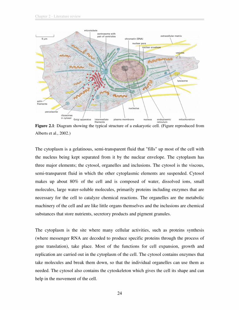
Figure 2.1: Diagram showing the typical structure of a eukaryotic cell. (Figure reproduced from
Alberts et al., 2002.)
The cytoplasm is a gelatinous, semi-transparent fluid that "fills" up most of the cell with
the nucleus being kept separated from it by the nuclear envelope. The cytoplasm has
three major elements; the cytosol, organelles and inclusions. The cytosol is the viscous,
semi-transparent fluid in which the other cytoplasmic elements are suspended. Cytosol
makes up about 80% of the cell and is composed of water, dissolved ions, small
molecules, large water-soluble molecules, primarily proteins including enzymes that are
necessary for the cell to catalyze chemical reactions. The organelles are the metabolic
machinery of the cell and are like little organs themselves and the inclusions are chemical
substances that store nutrients, secretory products and pigment granules.
The cytoplasm is the site where many cellular activities, such as proteins synthesis
(where messenger RNA are decoded to produce specific proteins through the process of
gene translation), take place. Most of the functions for cell expansion, growth and
replication are carried out in the cytoplasm of the cell. The cytosol contains enzymes that
take molecules and break them down, so that the individual organelles can use them as
needed. The cytosol also contains the cytoskeleton which gives the cell its shape and can
help in the movement of the cell.
Chapter 2 - Literature review
25
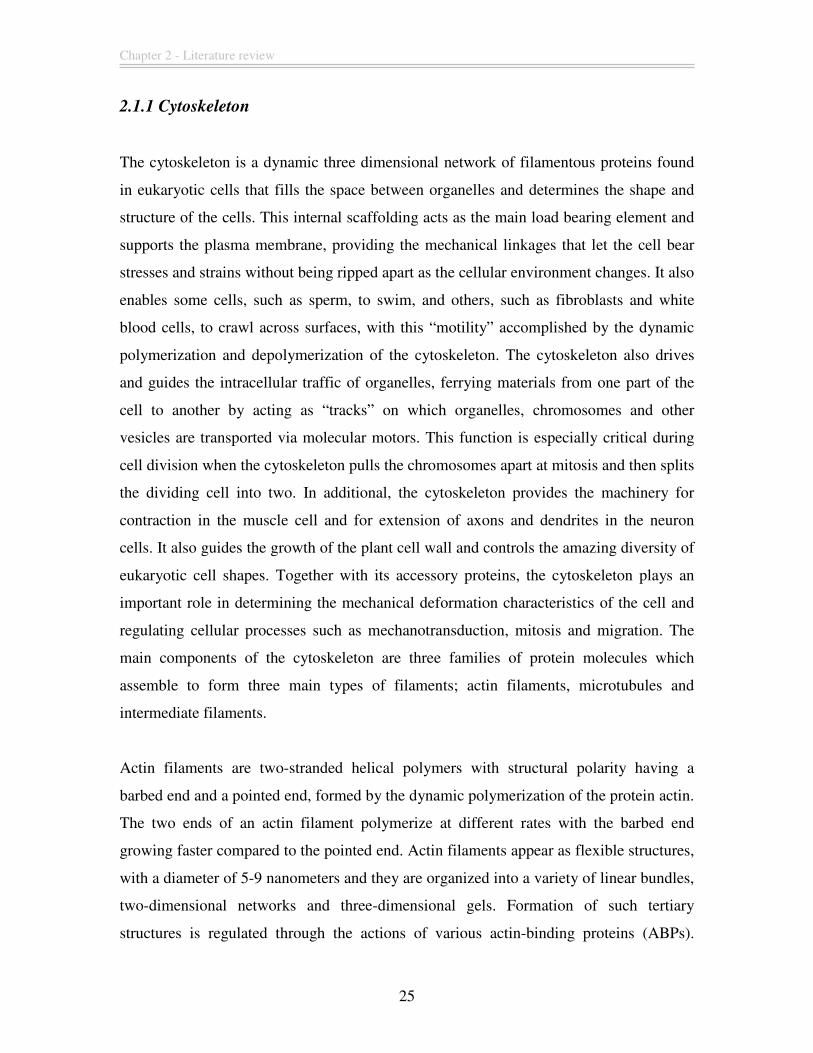
2.1.1 Cytoskeleton
The cytoskeleton is a dynamic three dimensional network of filamentous proteins found
in eukaryotic cells that fills the space between organelles and determines the shape and
structure of the cells. This internal scaffolding acts as the main load bearing element and
supports the plasma membrane, providing the mechanical linkages that let the cell bear
stresses and strains without being ripped apart as the cellular environment changes. It also
enables some cells, such as sperm, to swim, and others, such as fibroblasts and white
blood cells, to crawl across surfaces, with this “motility” accomplished by the dynamic
polymerization and depolymerization of the cytoskeleton. The cytoskeleton also drives
and guides the intracellular traffic of organelles, ferrying materials from one part of the
cell to another by acting as “tracks” on which organelles, chromosomes and other
vesicles are transported via molecular motors. This function is especially critical during
cell division when the cytoskeleton pulls the chromosomes apart at mitosis and then splits
the dividing cell into two. In additional, the cytoskeleton provides the machinery for
contraction in the muscle cell and for extension of axons and dendrites in the neuron
cells. It also guides the growth of the plant cell wall and controls the amazing diversity of
eukaryotic cell shapes. Together with its accessory proteins, the cytoskeleton plays an
important role in determining the mechanical deformation characteristics of the cell and
regulating cellular processes such as mechanotransduction, mitosis and migration. The
main components of the cytoskeleton are three families of protein molecules which
assemble to form three main types of filaments; actin filaments, microtubules and
intermediate filaments.
Actin filaments are two-stranded helical polymers with structural polarity having a
barbed end and a pointed end, formed by the dynamic polymerization of the protein actin.
The two ends of an actin filament polymerize at different rates with the barbed end
growing faster compared to the pointed end. Actin filaments appear as flexible structures,
with a diameter of 5-9 nanometers and they are organized into a variety of linear bundles,
two-dimensional networks and three-dimensional gels. Formation of such tertiary
structures is regulated through the actions of various actin-binding proteins (ABPs).
Chapter 2 - Literature review
26
Some examples of such actin-binding proteins are fimbrin and α-actinin, both
instrumental in the formation of linear bundles of actin filaments, termed “stress fibers”
and filamin, which connects actin filaments into a three-dimensional gel with filaments
joined at nearly right angles. Although actin filaments are dispersed throughout the cell,
they are mostly concentrated in the cortex, just beneath the plasma membrane. Their
importance is reflected in the fact that actin constitutes up to 10 percent of all the proteins
in most cells, and is present at even higher concentrations in muscle cells. Actin is also
thought to be the primary structural component of most cells for it responds rapidly to
mechanical perturbations and plays a critical role in the formation of leading-edge
protrusions during cellular migration.
Microtubules are polymers of α- and β-tubulin dimers which polymerize end to end into
protofilaments. These protofilaments then aligned in parallel to form a hollow cylindrical
filament. Typically, the protofilaments arrange themselves in an imperfect helix and the
cross section of a microtubule shows a ring of 13 distinct protofilaments. Microtubules
are long and straight and typically have one end attached to a single microtubule-
organizing center (MTOC) called a centrosome. With an outer diameter of 25 nanometers
and its tubular structure (tubular structures are more resistant to bending compared to
solid cylinders with the same amount of material per unit length); microtubules have a
much higher bending stiffness compared to actin filaments. Because of their high bending
stiffness, microtubules can also form long slender structures such as cilia and flagella.
During the process of cell division, microtubules are also involved in the segregation of
replicated chromosomes from the equatorial region of the cell (from a position called the
metaphase plate) to the polar regions through the formation of the mitotic spindles which
are complex cytoskeletal machinery. Microtubules are highly dynamic and undergo
constant polymerization and depolymerization. Their growth is asymmetric, similar to
that of actin, with polymerization typically occurring rapidly at one end and more slowly
at the other end.
Intermediate filaments are ropelike fibers with a diameter of around 10 nanometers; they
are made of intermediate filament proteins, which constitute a large and heterogeneous
Chapter 2 - Literature review
27
family containing more than fifty different members. They have in common a structure
consisting of a central α-helical domain that forms a coiled coil. The dimers then
assemble into a staggered array to form tetramers that connect end-to-end, forming
protofilaments which bundle into ropelike structures. One type of intermediate filaments
forms a meshwork called the nuclear lamina just beneath the inner nuclear membrane.
Other types extend across the cytoplasm, giving cells mechanical strength. In epithelial
tissues, they span the cytoplasm from one cell-cell junction to another, thereby
strengthening the entire epithelium.
In addition to the three main families of proteins described above, there are numerous
other proteins that influence the strength and integrity of the cytoskeleton such as the
actin-binding proteins (ABPs) introduced earlier. For example, a variety of capping,
binding, branching and severing proteins can affect both the rates of polymerization and
depolymerization of actin filaments within the cell. Through the regulation of such
accessory proteins, the cell is able to dynamically alter the structure of its cytoskeleton to
adapt to its mechanical environment or to perform certain specific functions. Vice-versa,
the cytoskeleton also serves as a mean of transmitting mechanical cues from the external
environment across the cell membrane and into the nucleus of the cell through different
signaling pathways. Such mechanical-biochemical coupling highlights the apparent
complexity in studying the cytoskeleton and the understanding of its mechanical
properties. Nevertheless, with advancement in experimental techniques (measurement of
forces on the picoNewton scale and length on the nanometer scale), we now possess more
tools that we can use to study cellular rheology and to gain a deeper understanding of the
working of the cytoskeleton.
2.2 Experimental Techniques
As we have seen, eukaryotic cells exhibit a heterogeneous structure that is totally
different from most everyday engineering materials, such as steel and concrete, that we
are more accustomed to. It is this very heterogeneous nature of biological cells that leads
to different experimental techniques being devised and used to probe the response of cells
Chapter 2 - Literature review
28
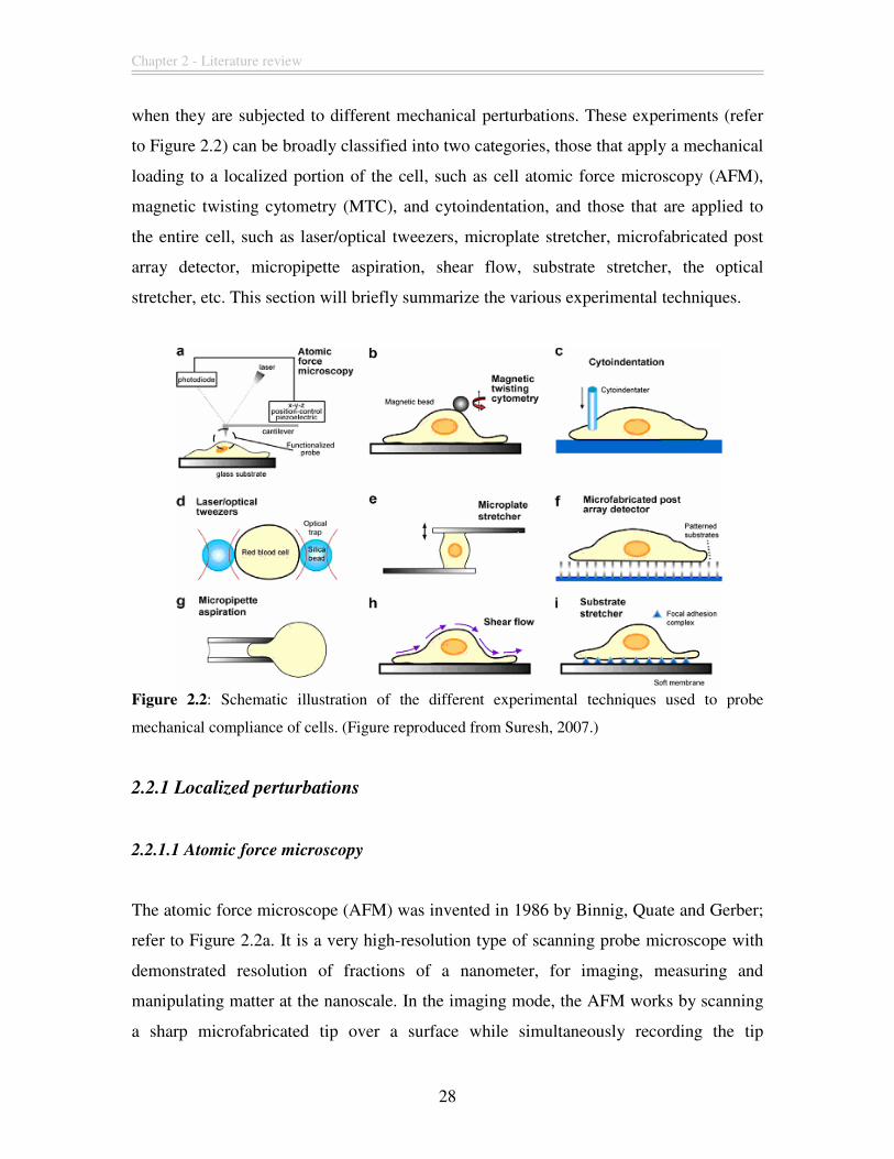
when they are subjected to different mechanical perturbations. These experiments (refer
to Figure 2.2) can be broadly classified into two categories, those that apply a mechanical
loading to a localized portion of the cell, such as cell atomic force microscopy (AFM),
magnetic twisting cytometry (MTC), and cytoindentation, and those that are applied to
the entire cell, such as laser/optical tweezers, microplate stretcher, microfabricated post
array detector, micropipette aspiration, shear flow, substrate stretcher, the optical
stretcher, etc. This section will briefly summarize the various experimental techniques.
Figure 2.2: Schematic illustration of the different experimental techniques used to probe
mechanical compliance of cells. (Figure reproduced from Suresh, 2007.)
2.2.1 Localized perturbations
2.2.1.1 Atomic force microscopy
The atomic force microscope (AFM) was invented in 1986 by Binnig, Quate and Gerber;
refer to Figure 2.2a. It is a very high-resolution type of scanning probe microscope with
demonstrated resolution of fractions of a nanometer, for imaging, measuring and
manipulating matter at the nanoscale. In the imaging mode, the AFM works by scanning
a sharp microfabricated tip over a surface while simultaneously recording the tip
Chapter 2 - Literature review
29
deflection. The deflection time course is then converted into an image of the surface
profile (Binnig et al., 1986). Imaging can be done in several different modes (Dufrene,
2003; Hansma et al., 1994; de Pablo et al., 1998) that are designed to minimize damage to
the sample surface being probed. In measurement and manipulation mode, the AFM tip
can be used to exert precisely controlled forces in selected locations and record the
corresponding sample displacements. The elastic moduli of the sample can be computed
using the Hertz relation which relates the force-displacement curves to the following
material properties; Young’s modulus, E, and Poisson’s ratio, ν, for a homogeneous,
semi-infinite elastic solid given the geometry of the needle tip.
When using an AFM with a sharp tip, the spatial inhomogeneities of cells (such as the
presence of stress fibers and microtubules) pose a problem because it makes interpreting
the results difficult. Thus, initial AFM elasticity measurements (Radmacher et al., 1993;
Rotsch et al., 1999; Nagao and Dvorak, 1999) were more qualitative in nature. Mahaffy
et al., (2000, 2004) developed a more quantitative technique using AFM by using
polystyrene beads of carefully controlled radius attached to the AFM tips. This creates a
well-defined probe geometry and provides for another parameter, namely bead radius to
control for the cellular inhomogeneities. The obvious limitation of the AFM though is
that manipulation can only occur on the surface of the cell and that measurement of
intracellular elasticity is not possible. Another limitation arises when the AFM is used to
measure the cell periphery in surface-attached cells. These regions, which are crucial for
cell motility, are usually too thin in thickness for the application of the standard Hertz
model. The Hertz model has since been modified to account for sample thickness and
boundary condition on the substrate (Mahaffy et al., 2004) which makes it possible to
estimate elastic moduli for thin lamellipodia of cells.
2.2.1.2 Magnetic twisting cytometry
Magnetic twisting cytometry (MTC) belongs to a broad class of experimental techniques
where an external magnetic field is used to apply forces and/or torques to either
paramagnetic (forces) or ferromagnetic (torques) beads that are either attached to the
Chapter 2 - Literature review
30
surface of the cell or inserted into the cytoplasm; refer to Figure 2.2b. The advantage of
using MTC to other experimental techniques in this class is that applying a pure torque to
magnetic particles avoids the difficulties of constructing a well-controlled field gradient
(it is difficult to establish homogeneous field gradients). The method most widely used
was pioneered by Valdberg and collegues (Valberg and Butler, 1987; Valberg and
Feldman, 1987; Wang et al., 1993) and consists of using a strong magnetic field pulse to
magnetize a large number of ferromagnetic particles that were previously attached to an
ensemble of cells. A weaker probe field oriented at 90 degrees to the induced dipoles then
causes the rotation, which is measured in a lock-in mode with a magnetometer. In a
homogeneous infinite medium, an effective shear modulus can be determined simply
from the angle rotated in response to an applied torque. However, on the surface of cells,
the conditions of the bead attachment are highly complex and the cellular body is more
heterogeneous than homogeneous. Therefore, MTC has been used mainly to determine
qualitative behavior, for a comparative studies of different cell types, and for studies of
relative changes in a given cell population.
2.2.1.3 Cytoindentation
The cytoindenter is another class of cell-indention experimental techniques where forces
are applied locally to the surface of living cells; refer to Figure 2.2c. This class of cell-
indention techniques includes the atomic force microscopy described above as well as the
cell poker developed by Duszyk et al. in 1989. Cytoindention was developed by Shin and
Athanasiou (1999) for measuring the visco-elastic characteristics of osteoblast-like cells
(MG63). It is designed to perform displacement controlled indentation tests on the
surface of individual cells. Briefly, the cytoindenter can apply incremental ramp-
controlled displacement perpendicularly to the top central portion of a single cell and
measure the corresponding normal, resistive force offered by the cell to the indenter. The
indenting probe is mounted onto the free edge of a cantilever beam, which serves as the
force-transducing system. Cantilever beam theory (which is one of the basic solutions in
mechanics) is utilized to determine this surface reaction force offered by the cell. The
advantage of this method is that the force resolution required in an experiment can be
Chapter 2 - Literature review
31
easily achieved by changing the length or cross-sectional area of the beam or choosing a
beam of different stiffness, thus allowing a precise and sensitive mean to determine the
cellular reaction force. The deflection of the cantilever beam is continuously monitored
and recorded during the experiment and these data are used to calculate the reaction force
on the cell surface.
2.2.2 Entire cell perturbations
2.2.2.1 Laser/optical tweezers
In this experimental technique, a laser beam is focused through a microscope objective
lens to attract and trap a high refractive index bead attached to the surface of the cell;
refer to Figure 2.2d. The resulting attractive force between the bead and the laser beam
pulls the bead towards the focal point of the laser trap. Two beads attached to
diametrically opposite ends of a cell can be trapped by two laser beams, thereby inducing
relative displacements between them, and hence uniaxially stretching the entire cell to
forces of up to several hundred picoNewtons (pN) (Sleep et al., 1999; Dao et al., 2003;
Lim et al., 2004). The attachment of these beads can be specific (the surfaces of the beads
are coated using a particular type of adhesion ligands to mediate specific binding to its
complementary cell surface receptors) or non-specific. Another variation of this method
involves a single trap, with the diametrically opposite end of the cell attached to a glass
plate which is displaced relative to the trapped bead (Suresh et al., 2005).
The laser/optical tweezers technique has the advantage that no mechanical access to the
cells is necessary (the mechanical perturbation is mediated through the attached beads)
and that beads of different sizes can be chosen to ensure that the site to be probed on the
cell can be chosen with relatively high resolution. However, one limitation of this
technique is the possible damage caused to the cell being probed through the heating
effect generated by the focused laser beam. This limitation usually places a bound on the
maximum power output of the laser used for trapping the bead, which in turn limits the
magnitude of the force generated by the laser tweezers.
Chapter 2 - Literature review
32
2.2.2.2 Microplate stretcher
This experimental technique was developed by Thoumine and co-workers (Thoumine and
Ott, 1997a; Thoumine et al., 1999) and it makes use of a pair of microplates; one rigid
plate that is mounted on a piezoelectric motor system and the other flexible plate that is
mounted on a fixed support, to apply forces to the entire cell; refer to Figure 2.2e. The
piezo-driven motors displace the rigid plate by a known distance to determine the strain
and the deflection of the flexible plate provides a measure of the strain and stress
imposed on the cell surface. The pair of microplates can be moved with respect to one
another in a variety of ways to impose compression, traction or oscillatory perturbation
on the cell to probe its mechanical responses. Depending on the cell type and the
experimental requirements, the two microplates can be coated separately or jointly with a
variety of cell-adhesion proteins to facilitate cell-surface adhesion.
The advantages of this technique are its simple geometry and a precise simultaneous
control of force and deformation. The experimental set-up also enables repeated
experiments to be carried out on the same cell which could possibly address the question
of whether cells retain a biochemical or rheological memory of past perturbations. One
limit of this technique is that the microplates used to manipulate cells in the experiments
are very adhesive and thereby promote cell spreading: this problem is partly overcome by
the fact that spreading is progressive and occurs on a time scale slower than that required
for deformation tests.
2.2.2.3 Microfabricated post array detector
This technique is used to manipulate and measure mechanical interactions between
adherent cells and their underlying substrates by using microfabricated arrays of
elastomeric, microneedle-like posts as substrate (Tan et al., 2003); refer to Figure 2.2f.
The compliance of the substrate can be varied by changing the geometry of the posts
(such as the cross-sectional shape) and the spacing of the posts, while keeping the other
surface properties constant. Cells attach to the arrays of micro-posts by spreading across
Chapter 2 - Literature review
33
and deflecting multiple posts, as they probe the mechanical compliance of the substrate
by locally deforming it with nanoNewton-scale traction forces. The deflections of the
individual posts occur independently of neighboring posts and can be used to directly
report the subcellular distribution of traction forces that is generated by the cell. For small
deflections, each post behaves like simple idealized beam such that the deflection is
directly proportional to the force applied by the attached cell. By tracking the deflection
of the arrays of posts, it is possible to generate a traction map showing the magnitude and
direction of the traction force exerted by the cell onto its substrate using this technique.
2.2.2.4 Micropipette aspiration
The micropipette aspiration technique has been used extensively to study the mechanical
properties of a variety of cells, including circulating cells such as erythrocytes (Evans,
1989), neutrophils (Sung et al., 1982; Dong et al., 1991; Ting-Beall et al., 1993),
adhesion-dependent cells such as fibroblasts (Thoumine and Ott, 1997b), endothelial cells
(Theret et al., 1998; Sato et al., 1990) and chondrocytes (Trickey et al., 2000; Guilak et
al., 2002); refer to Figure 2.2g. This technique involves the use of a small glass pipette to
apply controlled suction pressure to the cell surface while measuring the ensuing transient
deformation using video microscopy. Analyses of such experiments require the
development of a variety of theoretical models to interpret the response of the cells to the
micropipette aspiration. For instance, the analysis of Theret et al. (1988) for an infinite,
homogeneous half-space drawn into a micropipette gives the Young’s modulus, E, of the
cell as a function of the applied micropipette pressure, the length of aspiration of the cell
into the micropipette, the radius of the micropipette and a geometrical factor. The length
of the cell aspiration is measured at several increments and E can be subsequently
computed from the experimental data. A more detailed review of the various analytical
models of micropipette aspiration can be found in the review paper by Hochmuth (2000).
Subsequently in Chapter 5 of this thesis, we will present our simulation results based on
the tapered micropipette experiment (Needham and Hochmuth, 1992). This experiment is
a variation of the micropipette aspiration technique as described above.
Chapter 2 - Literature review
34
2.2.2.5 Shear flow
This technique can be used to extract the biomechanical response of population of cells
by monitoring the shear resistance of the cells to the imposed fluid flow (Usami et al.,
1993); refer to Figure 2.2h. Cells such as the vascular endothelial cells in the circulation
system or certain bone cells (osteocytes) within the bone matrix are regularly exposed to
fluid shear in the in-vivo environment and are suited to be studied using this technique.
Shear flow experiments involving laminar or turbulent flows are also commonly
performed using a cone-and-plate viscometer (Malek et al., 1995; Malek and Izumo,
1996) or a parallel plate flow chamber (Sato et al., 1996). For the cone-and-plate
viscometer, the shear stresses are generated by the rotation of the cone in the fluid
medium. Cells grown on the surface of the plate can be subjected to varying regimes of
shear stress dependent on the Reynolds number of the system. In the parallel plate flow
chamber, the flow circuit is composed of the chamber and two reservoirs, and filled with
the necessary culture medium. The flow of medium is driven by the hydrostatic pressure
difference between the two reservoirs so as to attain a constant shear stress. The
expression of key signaling proteins or the overall morphology of the cell population is
monitored in the experiment to determine the influence of the shear stress. One example
of such cellular response to shear stress can be seen in the distinct transformation in the
actin cytoskeleton, resulting in rearrangement of F-actin filaments into bundles of stress
fibers aligned in the direction of flow (Wechezak et al., 1985; Kim et al., 1989).
2.2.2.6 Substrate stretcher
This technique directly manipulates the substrate to which cells are adhered, hence
providing a mean of mechanical stimulation; refer to Figure 2.2i. The strains on the
substrate are imposed and measured using standard strain gauges or other low-resolution
displacement sensors, and global forces are calculated directly from strain gauge output
and/or experimentally determined substrate stiffness. The mechanics of cell spreading,
deformation and migration in response to the imposed deformation on the compliant
polymeric substrates to which the cells are attached through focal adhesion complexes
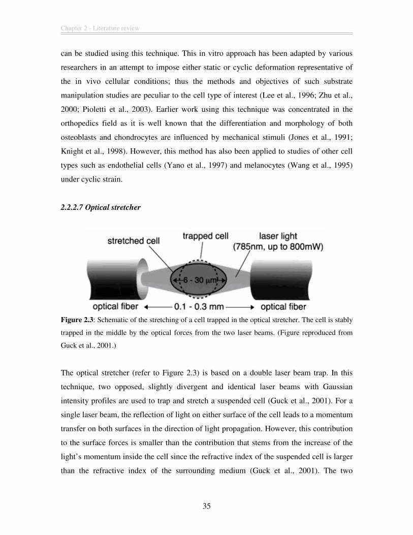
Chapter 2 - Literature review
35
can be studied using this technique. This in vitro approach has been adapted by various
researchers in an attempt to impose either static or cyclic deformation representative of
the in vivo cellular conditions; thus the methods and objectives of such substrate
manipulation studies are peculiar to the cell type of interest (Lee et al., 1996; Zhu et al.,
2000; Pioletti et al., 2003). Earlier work using this technique was concentrated in the
orthopedics field as it is well known that the differentiation and morphology of both
osteoblasts and chondrocytes are influenced by mechanical stimuli (Jones et al., 1991;
Knight et al., 1998). However, this method has also been applied to studies of other cell
types such as endothelial cells (Yano et al., 1997) and melanocytes (Wang et al., 1995)
under cyclic strain.
2.2.2.7 Optical stretcher
Figure 2.3: Schematic of the stretching of a cell trapped in the optical stretcher. The cell is stably
trapped in the middle by the optical forces from the two laser beams. (Figure reproduced from
Guck et al., 2001.)
The optical stretcher (refer to Figure 2.3) is based on a double laser beam trap. In this
technique, two opposed, slightly divergent and identical laser beams with Gaussian
intensity profiles are used to trap and stretch a suspended cell (Guck et al., 2001). For a
single laser beam, the reflection of light on either surface of the cell leads to a momentum
transfer on both surfaces in the direction of light propagation. However, this contribution
to the surface forces is smaller than the contribution that stems from the increase of the
light’s momentum inside the cell since the refractive index of the suspended cell is larger
than the refractive index of the surrounding medium (Guck et al., 2001). The two
Chapter 2 - Literature review
36
resulting surface forces on the front and back sides are opposite and tend to stretch the
cell (Guck et al., 2000). However, the asymmetry between the two surface forces leads to
a total force that acts on the center of the cell. If there is a second, identical ray of light
that passes through the cell from the opposite side, the total force acting on the cell will
be zero. But the forces on the surface generated by the two rays are additive thereby
stretching the cell. Using this experimental technique, Guck and co-workers (Guck et al.,
2005; Wottawah et al., 2005a, 2005b) are able to investigate the mechanical properties of
suspended fibroblast cells and their transformed cancerous counterparts. In Chapter 4 of
this thesis, we will present and discuss our simulation results based on modeling the
optical stretcher experiment. These simulation results will form the main contribution of
this thesis.
2.3 Overview of Mechanical Models
The different experimental techniques described above have led to a variety of different
mechanical models being developed to explain and interpret the data. This section will
give a brief overview of the different methodologies that were developed by various
researchers working on cellular mechanics. Broadly, the mechanical models used for
describing cell deformation can be classified into two categories, the
micro/nanostructural approach and the continuum approach. We will look at these two
approaches and highlight those mechanical models that are commonly used (refer to
Figure 2.4).
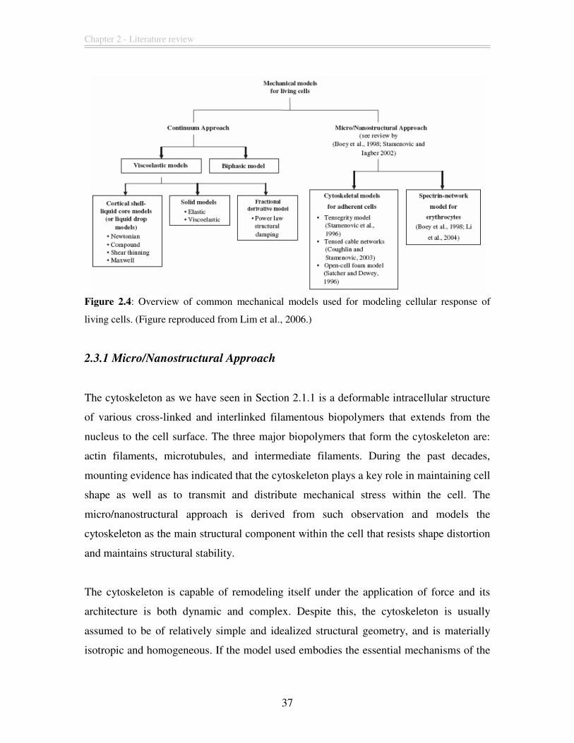
Chapter 2 - Literature review
37
Figure 2.4: Overview of common mechanical models used for modeling cellular response of
living cells. (Figure reproduced from Lim et al., 2006.)
2.3.1 Micro/Nanostructural Approach
The cytoskeleton as we have seen in Section 2.1.1 is a deformable intracellular structure
of various cross-linked and interlinked filamentous biopolymers that extends from the
nucleus to the cell surface. The three major biopolymers that form the cytoskeleton are:
actin filaments, microtubules, and intermediate filaments. During the past decades,
mounting evidence has indicated that the cytoskeleton plays a key role in maintaining cell
shape as well as to transmit and distribute mechanical stress within the cell. The
micro/nanostructural approach is derived from such observation and models the
cytoskeleton as the main structural component within the cell that resists shape distortion
and maintains structural stability.
The cytoskeleton is capable of remodeling itself under the application of force and its
architecture is both dynamic and complex. Despite this, the cytoskeleton is usually
assumed to be of relatively simple and idealized structural geometry, and is materially
isotropic and homogeneous. If the model used embodies the essential mechanisms of the
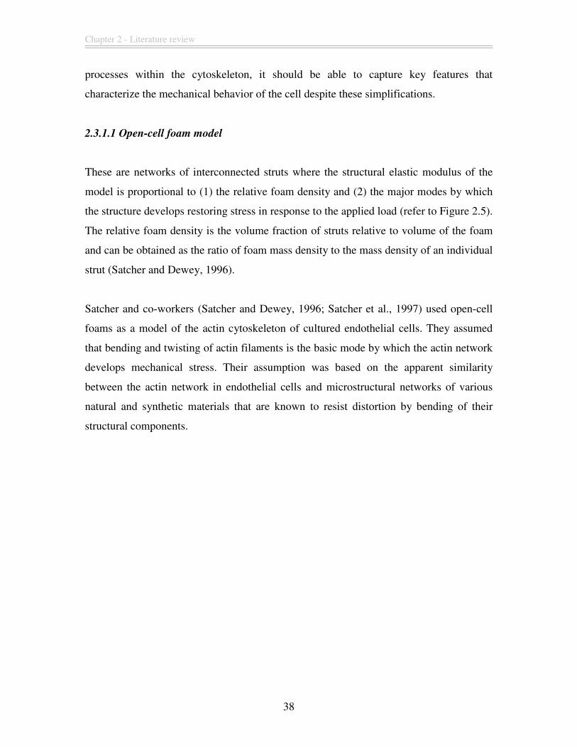
Chapter 2 - Literature review
38
processes within the cytoskeleton, it should be able to capture key features that
characterize the mechanical behavior of the cell despite these simplifications.
2.3.1.1 Open-cell foam model
These are networks of interconnected struts where the structural elastic modulus of the
model is proportional to (1) the relative foam density and (2) the major modes by which
the structure develops restoring stress in response to the applied load (refer to Figure 2.5).
The relative foam density is the volume fraction of struts relative to volume of the foam
and can be obtained as the ratio of foam mass density to the mass density of an individual
strut (Satcher and Dewey, 1996).
Satcher and co-workers (Satcher and Dewey, 1996; Satcher et al., 1997) used open-cell
foams as a model of the actin cytoskeleton of cultured endothelial cells. They assumed
that bending and twisting of actin filaments is the basic mode by which the actin network
develops mechanical stress. Their assumption was based on the apparent similarity
between the actin network in endothelial cells and microstructural networks of various
natural and synthetic materials that are known to resist distortion by bending of their
structural components.
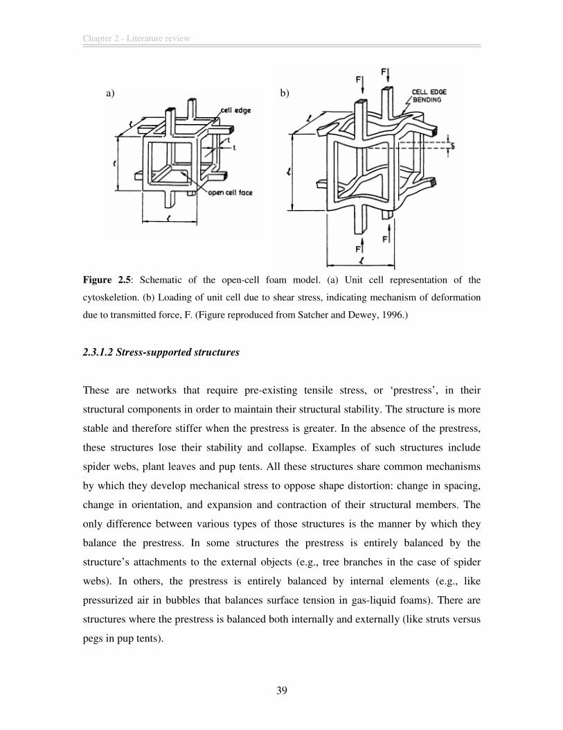
Chapter 2 - Literature review
39
Figure 2.5: Schematic of the open-cell foam model. (a) Unit cell representation of the
cytoskeletion. (b) Loading of unit cell due to shear stress, indicating mechanism of deformation
due to transmitted force, F. (Figure reproduced from Satcher and Dewey, 1996.)
2.3.1.2 Stress-supported structures
These are networks that require pre-existing tensile stress, or ‘prestress’, in their
structural components in order to maintain their structural stability. The structure is more
stable and therefore stiffer when the prestress is greater. In the absence of the prestress,
these structures lose their stability and collapse. Examples of such structures include
spider webs, plant leaves and pup tents. All these structures share common mechanisms
by which they develop mechanical stress to oppose shape distortion: change in spacing,
change in orientation, and expansion and contraction of their structural members. The
only difference between various types of those structures is the manner by which they
balance the prestress. In some structures the prestress is entirely balanced by the
structure’s attachments to the external objects (e.g., tree branches in the case of spider
webs). In others, the prestress is entirely balanced by internal elements (e.g., like
pressurized air in bubbles that balances surface tension in gas-liquid foams). There are
structures where the prestress is balanced both internally and externally (like struts versus
pegs in pup tents).
a) b)
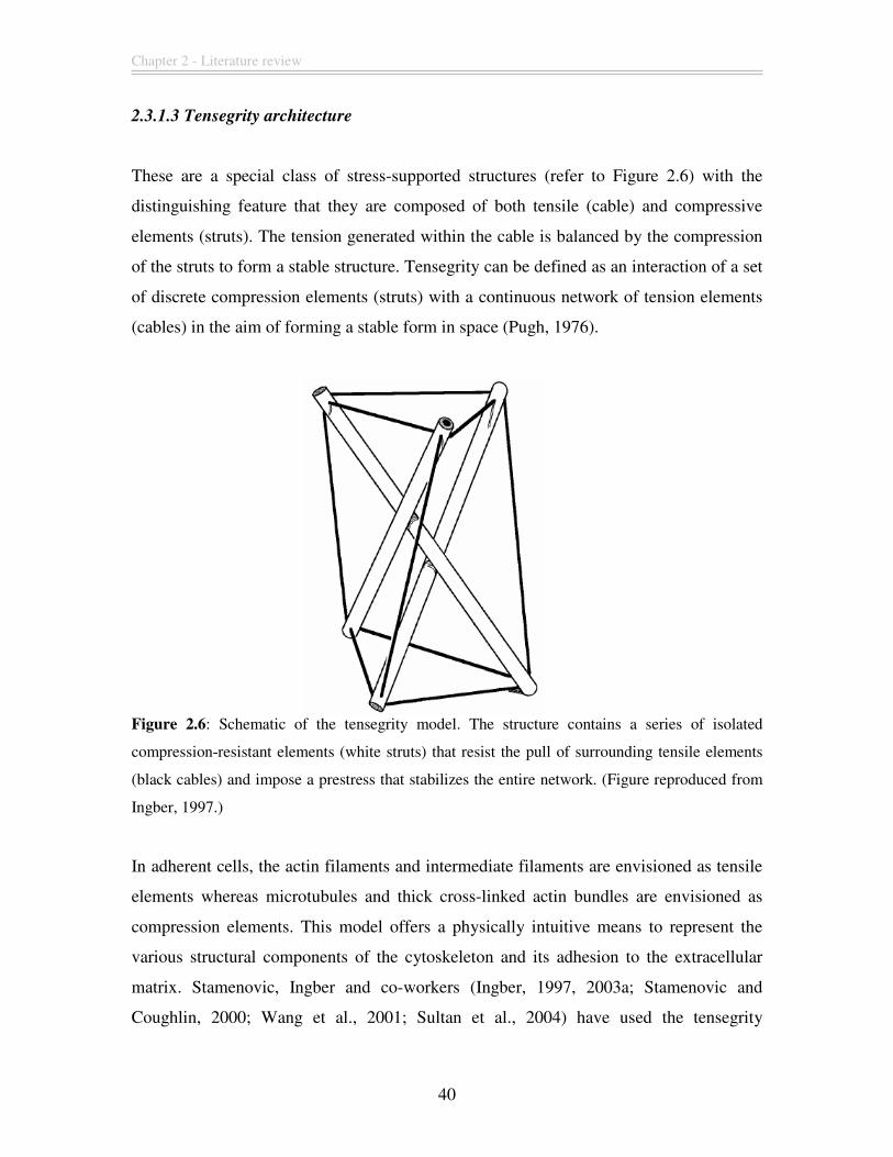
Chapter 2 - Literature review
40
2.3.1.3 Tensegrity architecture
These are a special class of stress-supported structures (refer to Figure 2.6) with the
distinguishing feature that they are composed of both tensile (cable) and compressive
elements (struts). The tension generated within the cable is balanced by the compression
of the struts to form a stable structure. Tensegrity can be defined as an interaction of a set
of discrete compression elements (struts) with a continuous network of tension elements
(cables) in the aim of forming a stable form in space (Pugh, 1976).
Figure 2.6: Schematic of the tensegrity model. The structure contains a series of isolated
compression-resistant elements (white struts) that resist the pull of surrounding tensile elements
(black cables) and impose a prestress that stabilizes the entire network. (Figure reproduced from
Ingber, 1997.)
In adherent cells, the actin filaments and intermediate filaments are envisioned as tensile
elements whereas microtubules and thick cross-linked actin bundles are envisioned as
compression elements. This model offers a physically intuitive means to represent the
various structural components of the cytoskeleton and its adhesion to the extracellular
matrix. Stamenovic, Ingber and co-workers (Ingber, 1997, 2003a; Stamenovic and
Coughlin, 2000; Wang et al., 2001; Sultan et al., 2004) have used the tensegrity
Chapter 2 - Literature review
41
architecture extensively to investigate cellular deformability. They have shown that the
tensegrity models can mimic a number of features observed in living adherent cells
during mechanical tests such as prestress-induced stiffening, strain hardening and the
effect of cell spreading on cell deformability. The assumptions from their studies are: (1)
the role of the actin network is to carry the prestress, thereby conferring shape stability to
the entire cell, (2) the role of the microtubules is to carry compression as they balance
prestress within the actin network. When the compression reaches a critical value, the
microtubules can buckle, thereby providing an additional degree of freedom to cell
deformability.
2.3.2 Continuum approach
The continuum approach treats the cell as comprising materials with certain continuum
properties and does not model the cytoskeleton as the main structural component of the
cell, unlike the micro/nanostructural approach. Instead, the appropriate constitutive
material models and parameters are derived from experimental data. Although this
approach is unlikely to shed light on the detailed molecular mechanical events occurring
at the protein level, it is easier and more straightforward to implement especially when
computing the biomechanical response at the cellular level. Nevertheless, a continuum
model can still provide insights into the stress and strain distribution within a cell when it
is subjected to mechanical loading and will be useful in determining the transmission of
these forces to the cytoskeleton and sub-cellular components.
2.3.2.1 Cortical shell-liquid core models
The cortical shell-liquid core models were first developed mainly to account for the
rheology of neutrophils undergoing micropipette aspiration. The Newtonian liquid drop
model, the compound Newtonian liquid drop model, the shear thinning liquid drop
model, and the Maxwell liquid drop model belong to this category.
Chapter 2 - Literature review
42
2.3.2.1.1 Newtonian liquid drop model
The Newtonian liquid drop model (refer to Figure 2.7) was developed in an attempt to
simulate the flow of liquid-like cells, such as leukocytes, into a micropipette (Yeung and
Evans, 1989). Leukocytes behave like a liquid drop and adopt a spherical shape when
suspended. They can deform continuously into a micropipette with a smaller diameter
when the pressure difference exceeds a certain threshold and can recover their initial
spherical shape upon release (Evans and Kukan, 1984). In this model, the cell interior is
assumed to be a homogeneous Newtonian viscous liquid and the cell cortex is taken as an
anisotropic viscous fluid layer with static tension but without any bending resistance.
Further, the velocity field is assumed continuous at the interface between the cortical
layer and the cytoplasmic core.
2.3.2.1.2 Compound Newtonian liquid drop model
Eukaryotic cells are composed of three main components: (1) the cell membrane, (2) the
cytoplasm (which includes the cytosol, cytoskeleton and various suspended organelles),
and (3) a nucleus (a nucleoplasm with genetic materials bounded by a nuclear envelope).
It has been demonstrated that the cell nucleus is many times stiffer and more viscous than
the surrounding cytoplasm (Guilak et al., 2000; Caille et al., 2002), thus a more complex
model comprising heterogeneous parts is needed to accurately reflect the physical
makeup of the cell. The compound liquid drop model (Dong et al., 1991; Hochmuth et
al., 1993) comprises a three-layer structure (refer to Figure 2.7). The cell nucleus is
modeled as a smaller and more viscous Newtonian liquid drop bounded by a constant
surface tension, 2T . It is enclosed within the cytoplasm which is modeled with a larger
but less viscous Newtonian liquid droplet with a constant surface tension, 1T .
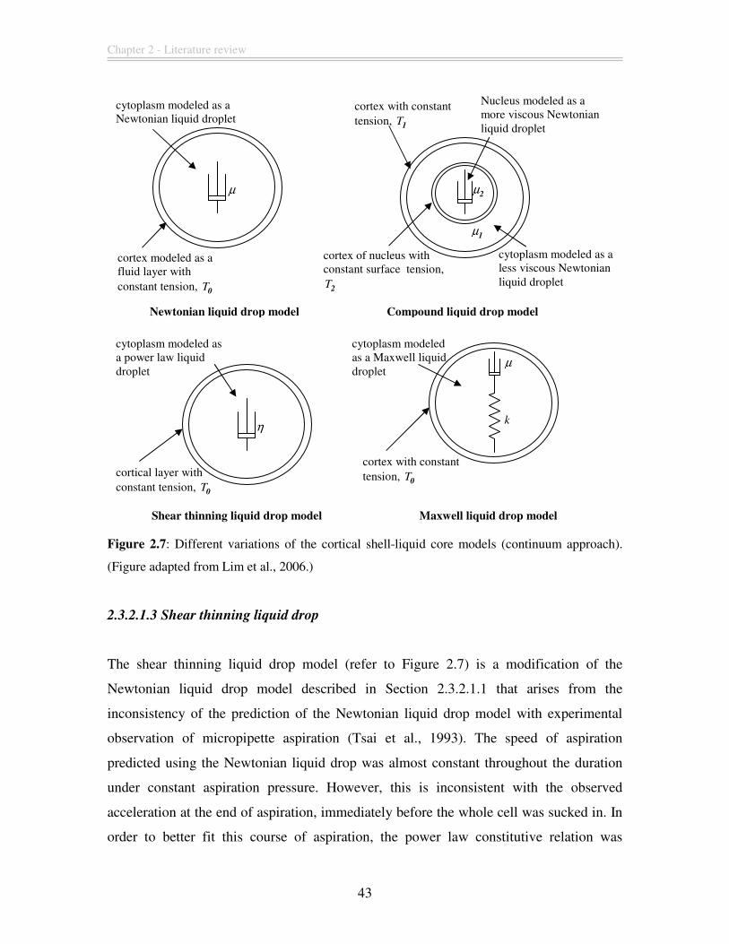
Chapter 2 - Literature review
43
Figure 2.7: Different variations of the cortical shell-liquid core models (continuum approach).
(Figure adapted from Lim et al., 2006.)
2.3.2.1.3 Shear thinning liquid drop
The shear thinning liquid drop model (refer to Figure 2.7) is a modification of the
Newtonian liquid drop model described in Section 2.3.2.1.1 that arises from the
inconsistency of the prediction of the Newtonian liquid drop model with experimental
observation of micropipette aspiration (Tsai et al., 1993). The speed of aspiration
predicted using the Newtonian liquid drop was almost constant throughout the duration
under constant aspiration pressure. However, this is inconsistent with the observed
acceleration at the end of aspiration, immediately before the whole cell was sucked in. In
order to better fit this course of aspiration, the power law constitutive relation was
cortical layer with constant tension, 0T
η
Shear thinning liquid drop model
cytoplasm modeled as a power law liquid droplet
Maxwell liquid drop model
cortex with constant tension, 0T
cytoplasm modeled as a Maxwell liquid droplet
µ
k
cortex of nucleus with constant surface tension,
2T
cortex with constant tension, 1T
Compound liquid drop model
Nucleus modeled as a more viscous Newtonian liquid droplet
2µ
1µ
cytoplasm modeled as a less viscous Newtonian liquid droplet
µ
Newtonian liquid drop model
cortex modeled as a fluid layer with constant tension, 0T
cytoplasm modeled as a Newtonian liquid droplet
Chapter 2 - Literature review
44
incorporated into the cortical shell-liquid core model (Tsai et al., 1993). In this model, the
cortex of the cell is still modeled as a layer with constant tension, 0T while the cytoplasm
is modeled as a shear thinning liquid governed by a power law.
2.3.2.1.4 Maxwell liquid drop model
The Maxwell liquid drop model (refer to Figure 2.7) was developed to account for the
small or initial deformation phase in order to explain the initial rapid elastic-like entry
during the micropipette aspiration of the cell (Dong et al., 1988). The cell is modeled as a
Maxwell liquid droplet bounded by a constant tension, 0T . The main qualitative
difference between this model and the other cortical shell-liquid core models is that the
Maxwell liquid drop model contains an elastic element. Its success lies in explaining the
initial jump in deformation during micropipette aspiration and the initial rapid elastic
rebound during recovery of cells held in the pipette for a very short time (less than 5
seconds).
2.3.2.2 Solid models
In solid models, the entire cell is usually assumed as homogeneous without considering
the distinct cortical layer and nucleus. The constitutive material models used include the
incompressible elastic solid or the viscoelastic solid. The experimental basis for the solid
models is that equilibrium can usually be achieved after a certain amount of loading. For
example, endothelial cells exposed to fluid shear stress are known to retain an elongated
configuration even after detachment (Theret et al., 1988).
2.3.2.2.1 Linear elastic solid model
The linear elastic model is a simplification of the viscoelastic model where the time
factor has been neglected. The constitutive equation for linear elastic, isotropic material
can be defined using two parameters: E, the Young’s modulus, otherwise known as the
elastic modulus and ν, the Poisson’s ratio. Unfortunately, the linear elastic model is
Chapter 2 - Literature review
45
generally inadequate for describing the mechanics of cells because cells are known to
exhibit non-linear responses during deformation which is dependent on both the loading
rate and loading history (Thoumine and Ott, 1997a; Wottawah et al., 2005a). Therefore,
these experimental observations limit the usefulness of solutions obtained from the linear
elastic model in predicting cellular responses to mechanical perturbations. However, the
linear elastic solution can serve as a basis for a viscoelastic solution according to the
corresponding principle (Fung, 1965) where the set of differential equations obtained
from the viscoelastic model are reduced to algebraic equations through the Laplace
transformation.
2.3.2.2.2 Viscoelastic solid model
The viscoelastic solid model treats the entire cell as a continuum described by a
constitutive material equation that is dependent on the type of viscoelastic model chosen.
Different cellular responses can be obtained through the use of either a solid viscoelastic
model or a liquid viscoelastic model with a varying number of parameters. The key
difference between the solid and liquid model can be seen in their long term creep
response under constant loading. Creep for the solid viscoelastic model will reach a
plateau while creep for the liquid model will increase indefinitely with time. One
common viscoelastic model that is used for modeling cellular deformation is the standard
linear solid which is characterized by 3 parameters (Sato et al., 1996; Lo and Ferrier,
1999; Guilak et al., 2000; Koay et al., 2003) (the standard linear solid will be further
elaborated in Section 3.2 of the thesis). Though the viscoelastic model ignores all the
micro-structural details about the cell interior, it has the advantage that it leads to a set of
less complicated equations that can be solved. Hence, this approach can be useful in
describing overall cellular responses based on experimental observation. This is also the
main approach followed in this thesis. The numerical methods used to implement this
approach will be discussed in Chapter 3.
Chapter 2 - Literature review
46
2.3.2.2.3 Power-law dependent model
The power-law dependent model is another class of models that is based on the
experimental observation of the dynamic responses of the cytoskeleton to mechanical
perturbation (Fabry et al., 2001; Hoffman et al., 2006; Trepat et al., 2007). These
experiments indicate that the cell response over a broad frequency spectrum is governed
by a ubiquitous mechanical behavior called power-law rheology which is an intrinsic
feature of many soft materials such as emulsions, pastes, foams and colloids (Mason and
Weitz, 1995; Weeks et al., 2000; Cloitre et al., 2000, 2003). These materials which all fall
in the category of soft glassy materials (Sollich et al., 1997) are composed of numerous
discrete elements that experience weak interactions with inherently disordered and
metastable microstructural geometry. The complex dynamics exhibited by these
materials, far from thermodynamic equilibrium, exhibits power-law frequency
dependence with no single characteristic frequency or timescale. This feature is
completely opposite from that of viscoelastic models described in the previous section, in
that viscoelastic models constructed using combinations of spring and dashpots will
exhibit distinct characteristic frequencies or timescales. The number of characteristic
frequencies or timescales of a viscoelastic model is dependent on the number of
underlying spring and dashpot components. For soft glassy materials, their shear modulus
G* (which measures the material resistance to shear deformation and arises in the
generalized Hooke’s law) is complex and frequency dependent. G* can be separated into
two components, the storage modulus, G’ (the real part of G* corresponding to the elastic
response) and the loss modulus, G’’ (the imaginary part of G* corresponding to the
viscous response). Both of these moduli have been shown to exhibit weak power-law
dependence on the frequency of perturbation (Fabry et al., 2001; Trepat et al., 2007).
Chapter 3 - Numerical method
47
Chapter 3. Numerical method
This chapter gives an overview of the numerical method used in this thesis, the finite
element method. The finite element method has a relatively short history, with the term
“finite element” being introduced for the first time by Clough in 1960 in a paper titled
“The finite element method in plane stress analysis”. Prior to this date, the earlier works
of Ritz (1909) and Courant (1943) had already established some of the principles of
modern day finite element methods. Nevertheless, it should be noted that the finite
element method was not invented or developed by just a single individual but by many
different researchers working either together in groups or independently from one
another. Some of the prominent names (definitely not an exhaustive list) associated with
the development of the modern day finite element method include M.J. Turner, B.M.
Irons, R.J. Melosh, E.L. Wilson, J.H. Argyris, H.C. Martin and O.C. Zienkiewicz.
The basic concept of the finite element method is to establish approximate solutions in
terms of unknown parameters in sub-regions of the problem called “elements” and then
to deduce an approximate solution for the whole domain by enforcing certain relations
among the solution of all of the elements. For example, in the field of structural analysis,
the concept of the finite element method is to express the displacement and internal
forces at the selected nodal points of individual structural components in the form of a
system of algebraic equations. The unknowns for the equations can be the nodal
displacements, the nodal internal forces or both. In a similar manner, the finite element
method has been extended to other fields of engineering involving fluid mechanics,
electromagnetism, heat transfer, among others, and is one of the most commonly used
numerical methods today.
The first section of this chapter will cover the formulation of the finite element method in
linear elasticity, where the material constitutive equations are described by the
generalized Hooke’s law. We also make the assumption that we are working in the small
strain regime, in a simplified two dimensional plain strain setting. In the subsequent
sections, we will look into extending this formulation to include viscoelastic material
Chapter 3 - Numerical method
48
constitutive equations. The rationale for such an approach is that we want to use the finite
element method to model single cell deformation whereby cellular responses to
mechanical perturbations have been shown to be dependent on both the loading rate and
loading history (Thoumine and Ott, 1997a; Wottawah et al., 2005a). This chapter will
then conclude with an extension of the formulation of the finite element method from a
two dimensional plain strain setting to a three dimensional setting using an axisymmetric
stress analysis.
3.1 Linear finite element scheme
3.1.1 Preliminary
This section starts by describing the numerical scheme implemented to model the
dynamic deformation of a continuum solid with isotropic material properties using the
finite element method. In general, the governing equation of motion for a continuum
solid analyzed under dynamic loading conditions (Zienkiewicz and Taylor, 1989) is given
by the following equation:
extMu + Cu + Ku = f&& & (1)
where M is the mass matrix, C is the damping matrix, K is the stiffness matrix, extf is
the external load (which can be varying in time) and u is the material displacement
vector. The notations of the various quantities are based on the following conventions.
Scalars are given in italics (e.g. ε ,u ). Vectors and tensors are in bold-face (e.g. B ,u ).
We assumed that the external loading is known and that the only unknown variable in the
above equation is the displacement vector u . Thus we want to solve for the displacement
of the body as it deforms under an externally applied load. We also further assume the
continuity of the displacement field within the body and that no breakages or fractures
occur during the course of the loading. In order to incorporate viscoelastic material
properties into our numerical scheme at a later stage, Equation (1) can be written in the
following alternative form which does not require that the material be linearly elastic:
Chapter 3 - Numerical method
49
int extMu + Cu + R = f&& & (2)
where intR is the internal force vector.
3.1.2 Linear elastic constitutive equations
To relate the strain in the body to the corresponding displacement field, we make the
assumptions that we are working in the small displacement regime (which implies that
the corresponding strain is small) and that the numerical analysis is conducted in a
simplified two dimensional plain strain setting. We will subsequently extend our analysis
to a three dimensional setting using an axisymmetric formulation and details of this
formulation will be covered in Section 3.5 of this chapter. For the remainder of this
section until Section 3.5, we will be working in a two dimensional plain strain setting.
The assumption that we are working in the small strain regime places considerable
limitation on the types of experiments we can model using our finite element formulation.
However, given the exceptional complexity of the mechanical behavior of cells, a finite
element model incorporating truly large strain and geometrical non-linearity formulation
would take more time than was available for this PhD research project. This is because
we had chosen to write our own finite element code instead of using commercially
available packages. While commercial finite element packages do offer the advantage of
ease of use, our concerns were that most of these packages are “black box” programs
which do not allow the users much control over the inner working of the code. In view of
this, we decided to implement our own finite element code to incorporate viscoelastic
material non-linearity to model cellular responses in the optical stretcher (refer to Chapter
4) and tapered micropipette (refer to Chapter 5) so that we have complete control over
our formulation. We acknowledge the limitations of our current finite element model but
we are confident that the results obtained from our model can still contribute to the
understanding of cellular rheology.
Following our assumptions, we can define Cauchy’s infinitesimal strain tensor
(Zienkiewicz and Taylor, 1989; Fung and Tong, 2001) as follows:
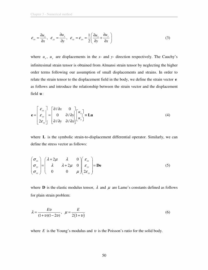
Chapter 3 - Numerical method
50
1, ,
2y yx x
xx yy xy yx
u uu u
x y y xε ε ε ε
∂ ∂ ∂ ∂= = = = +
∂ ∂ ∂ ∂ (3)
where x
u , y
u are displacements in the x- and y- direction respectively. The Cauchy’s
infinitesimal strain tensor is obtained from Almansi strain tensor by neglecting the higher
order terms following our assumption of small displacements and strains. In order to
relate the strain tensor to the displacement field in the body, we define the strain vector e
as follows and introduce the relationship between the strain vector and the displacement
field u :
/ 0
0 /
2 / /
xx
x
yy
y
xy
xu
yu
y x
ε
ε
ε
∂ ∂ = = ∂ ∂ ≡ ∂ ∂ ∂ ∂
e Lu (4)
where L is the symbolic strain-to-displacement differential operator. Similarly, we can
define the stress vector as follows:
2 0
2 0
0 0 2
xx xx
yy yy
xy xy
σ λ µ λ ε
σ λ λ µ ε
σ µ ε
+
= + =
De (5)
where D is the elastic modulus tensor, λ and µ are Lame’s constants defined as follows
for plain strain problem:
( ),
(1 )(1 2 ) 2 1
E Eυλ µ
υ υ υ= =
+ − + (6)
where E is the Young’s modulus and υ is the Poisson’s ratio for the solid body.
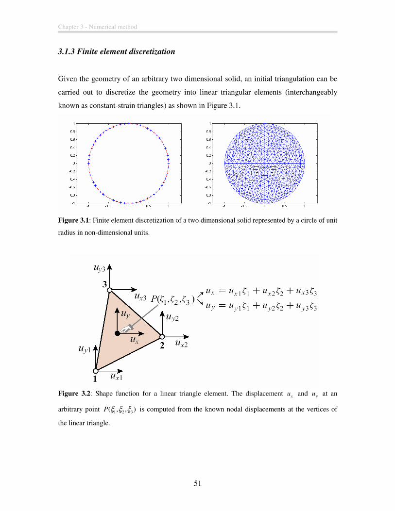
Chapter 3 - Numerical method
51
3.1.3 Finite element discretization
Given the geometry of an arbitrary two dimensional solid, an initial triangulation can be
carried out to discretize the geometry into linear triangular elements (interchangeably
known as constant-strain triangles) as shown in Figure 3.1.
Figure 3.1: Finite element discretization of a two dimensional solid represented by a circle of unit
radius in non-dimensional units.
Figure 3.2: Shape function for a linear triangle element. The displacement
xu and yu at an
arbitrary point 1 2 3( , , )P ξ ξ ξ is computed from the known nodal displacements at the vertices of
the linear triangle.
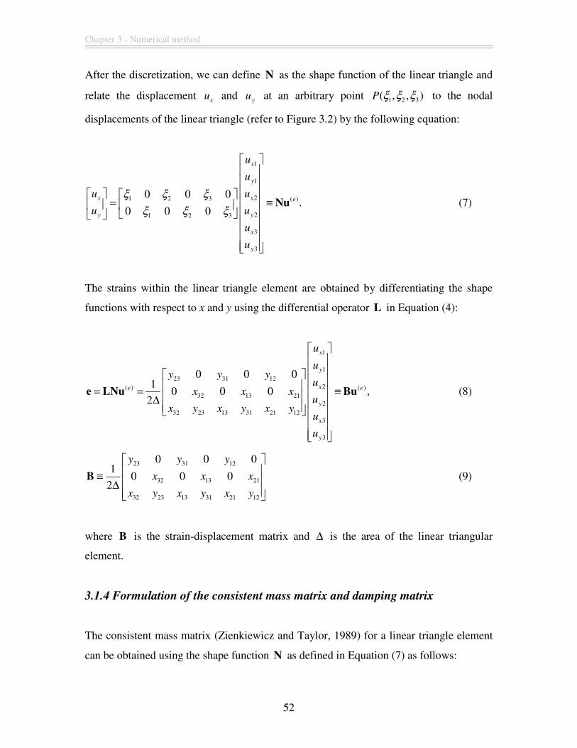
Chapter 3 - Numerical method
52
After the discretization, we can define N as the shape function of the linear triangle and
relate the displacement x
u and y
u at an arbitrary point 1 2 3( , , )P ξ ξ ξ to the nodal
displacements of the linear triangle (refer to Figure 3.2) by the following equation:
1
1
21 2 3 ( )
21 2 3
3
3
0 0 0.
0 0 0
x
y
x x e
y y
x
y
u
u
u u
u u
u
u
ξ ξ ξ
ξ ξ ξ
= ≡
Nu (7)
The strains within the linear triangle element are obtained by differentiating the shape
functions with respect to x and y using the differential operator L in Equation (4):
1
1
23 31 122( ) ( )
32 13 212
32 23 13 31 21 123
3
0 0 01
0 0 0 ,2
x
y
xe e
y
x
y
u
uy y y
ux x x
ux y x y x y
u
u
= = ≡ ∆
e LNu Bu (8)
23 31 12
32 13 21
32 23 13 31 21 12
0 0 01
0 0 02
y y y
x x x
x y x y x y
≡ ∆
B (9)
where B is the strain-displacement matrix and ∆ is the area of the linear triangular
element.
3.1.4 Formulation of the consistent mass matrix and damping matrix
The consistent mass matrix (Zienkiewicz and Taylor, 1989) for a linear triangle element
can be obtained using the shape function N as defined in Equation (7) as follows:
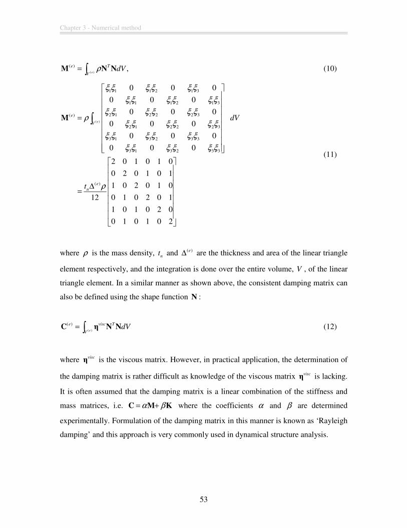
Chapter 3 - Numerical method
53
( )
( ) ,e
e T
VdVρ= ∫M N N (10)
( )
1 1 1 2 1 3
1 1 1 2 1 3
2 1 2 2 2 3( )
2 1 2 2 2 3
3 1 3 2 3 3
3 1 3 2 3 3
( )
0 0 0
0 0 0
0 0 0
0 0 0
0 0 0
0 0 0
2 0 1 0 1 0
0 2 0 1 0 1
1 0 2 0 1 0
0 1 0 2 0 112
1 0 1 0 2 0
0 1 0 1 0 2
e
e
V
e
n
dV
t
ξ ξ ξ ξ ξ ξ
ξ ξ ξ ξ ξ ξ
ξ ξ ξ ξ ξ ξρ
ξ ξ ξ ξ ξ ξ
ξ ξ ξ ξ ξ ξ
ξ ξ ξ ξ ξ ξ
ρ
=
∆
=
∫M
(11)
where ρ is the mass density, n
t and ( )e∆ are the thickness and area of the linear triangle
element respectively, and the integration is done over the entire volume, V , of the linear
triangle element. In a similar manner as shown above, the consistent damping matrix can
also be defined using the shape function N :
( )
( )e
e visc T
VdV= ∫C η N N (12)
where viscη is the viscous matrix. However, in practical application, the determination of
the damping matrix is rather difficult as knowledge of the viscous matrix viscη is lacking.
It is often assumed that the damping matrix is a linear combination of the stiffness and
mass matrices, i.e. α β= +C M K where the coefficients α and β are determined
experimentally. Formulation of the damping matrix in this manner is known as ‘Rayleigh
damping’ and this approach is very commonly used in dynamical structure analysis.
Chapter 3 - Numerical method
54
3.1.5 Numerical solution techniques
An explicit direct integration method can be employed to solve Equation (2). Writing
Equation (2) at a specific instant of time, we obtain:
{ } { } { } { }int ext
n n n n+ + =M u C u R F&& & (13)
where { }n
• denotes the values of the variable at the specific time instant n .
Using the central-difference method to approximate the velocity and acceleration, we
obtain:
{ } { } { }( )
{ } { } { } { }( )
1 1
2 1 1
1,
21
2 .
n n n
n n n n
t
t
+ −
+ −
= −∆
= − +∆
u u u
u u u u
&
&&
(14)
Combining Equations (13) and (14),
{ } { } { } { } { }( ) { }ext int
2 21 1 1
1 1 1 12 .
2 2n n n nn nt t t t+ − −
+ = − + − + ∆ ∆ ∆ ∆
M C u F R M u u C u (15)
Starting the method from n = 0 requires { }1−
u which can be computed from known initial
conditions { }0
u and { }0
u& from the equation below:
{ } { } { } { }2
1 0 0 02
tt
−
∆= − ∆ +u u u u& && (16)
where terms with 3t∆ and higher powers are omitted. The term { }
0u&& is obtained using
Equation (13):
Chapter 3 - Numerical method
55
{ } { } { } { }1 ext int
0 00 0( ).−= − −u M F R C u&& & (17)
Equation (15) is conditionally stable and requires t∆ such that:
tω
∆ ≤max
2 (18)
where maxω is the highest natural frequency of 2det( ) 0ω− =K M .
Similarly an implicit technique can also be employed to solve Equation (2). One of the
most widely used family of implicit methods of direct time integration for solving semi-
discrete equations of motion is Newmark’s family of methods (Newmark, 1959). The
Newmark method is based on the following assumptions:
{ } { } { } { }1 1
(1 ) ,n n n n
t γ γ+ +
= + ∆ − + u u u u& & && && (19)
{ } { } { } { } { }2
1 1( ) (0.5 )
n n n n nt t β β
+ + = + ∆ + ∆ − + u u u u u& && && (20)
where the parameters β and γ determine the stability and accuracy of the algorithm.
Solving Equation (20) for { }1n+
u&& in terms of { }1n+
u and then substituting for { }1n+
u&& in
Equation (19), we can obtain equations for { }1n+
u&& and { }1n+
u& each in terms of the
unknown displacements { }1n+
u only. Writing Equation (1) at a specific instant of time
and substituting the expressions for { }1n+
u&& and { }1n+
u& gives a system of simultaneous
equations which can be solved for { }1n+
u :
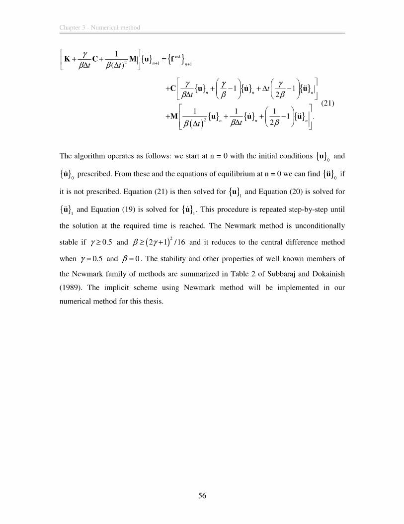
Chapter 3 - Numerical method
56
{ } { }ext
2 1 1
1
( ) n nt t
γ
β β + +
+ + = ∆ ∆
K C M u f
{ } { } { }
( ){ } { } { }2
1 12
1 1 11 .
2
n n n
n n n
tt
tt
γ γ γ
β β β
β ββ
+ + − + ∆ −
∆
+ + + −
∆∆
C u u u
M u u u
& &&
& &&
(21)
The algorithm operates as follows: we start at n = 0 with the initial conditions { }0
u and
{ }0
u& prescribed. From these and the equations of equilibrium at n = 0 we can find { }0
u&& if
it is not prescribed. Equation (21) is then solved for { }1
u and Equation (20) is solved for
{ }1
u&& and Equation (19) is solved for { }1
u& . This procedure is repeated step-by-step until
the solution at the required time is reached. The Newmark method is unconditionally
stable if 0.5γ ≥ and ( )2
2 1 /16β γ≥ + and it reduces to the central difference method
when 0.5γ = and 0β = . The stability and other properties of well known members of
the Newmark family of methods are summarized in Table 2 of Subbaraj and Dokainish
(1989). The implicit scheme using Newmark method will be implemented in our
numerical method for this thesis.
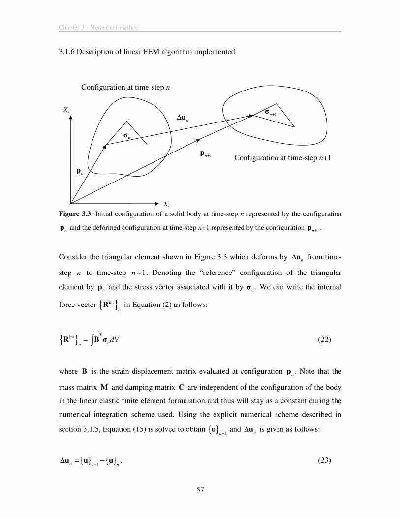
Chapter 3 - Numerical method
57
3.1.6 Description of linear FEM algorithm implemented
Figure 3.3: Initial configuration of a solid body at time-step n represented by the configuration
np and the deformed configuration at time-step n+1 represented by the configuration 1n+p .
Consider the triangular element shown in Figure 3.3 which deforms by n
∆u from time-
step n to time-step 1n + . Denoting the “reference” configuration of the triangular
element by n
p and the stress vector associated with it by nσ . We can write the internal
force vector { }int
nR in Equation (2) as follows:
{ }intT
nn
dV= ∫R B σ (22)
where B is the strain-displacement matrix evaluated at configuration n
p . Note that the
mass matrix M and damping matrix C are independent of the configuration of the body
in the linear elastic finite element formulation and thus will stay as a constant during the
numerical integration scheme used. Using the explicit numerical scheme described in
section 3.1.5, Equation (15) is solved to obtain { }1n+
u and n
∆u is given as follows:
{ } { }1
.n n n+∆ = −u u u (23)
X2
Configuration at time-step n
Configuration at time-step n+1
np
1n+p
n∆u
nσ
1n+σ
X1
Chapter 3 - Numerical method
58
The new “deformed” configuration of the triangular element in time-step 1n + is denoted
by 1n+p and is given by:
1 .n n n+ = + ∆p p u (24)
The new stress vector 1n+σ associated with the “deformed” configuration 1n+p is given
by:
( )1n n n+ = + ∆σ σ σ (25)
where n
∆σ is the incremental stress vector associated with the incremental deformation
n∆u and is given by:
n n n∆ = ∆ = ∆σ D e DB u (26)
and B is the strain-displacement matrix evaluated at configuration n
p and D is the
elastic modulus tensor.
3.2 Viscoelastic finite element formulation using the generalized
Maxwell model.
This section will extend the linear elastic finite element formulation described in the
previous section to include viscoelastic material constitutive equations. This is done by
using the generalized Maxwell model to represent the underlying structure of the solid body
under analysis. Finally, we showed that the standard linear solid (a common viscoelastic solid
model used for modeling cellular deformation, refer to Section 2.3.2.2.2) can be obtained
from simplifying the equations of the generalized Maxwell model. We will then use the
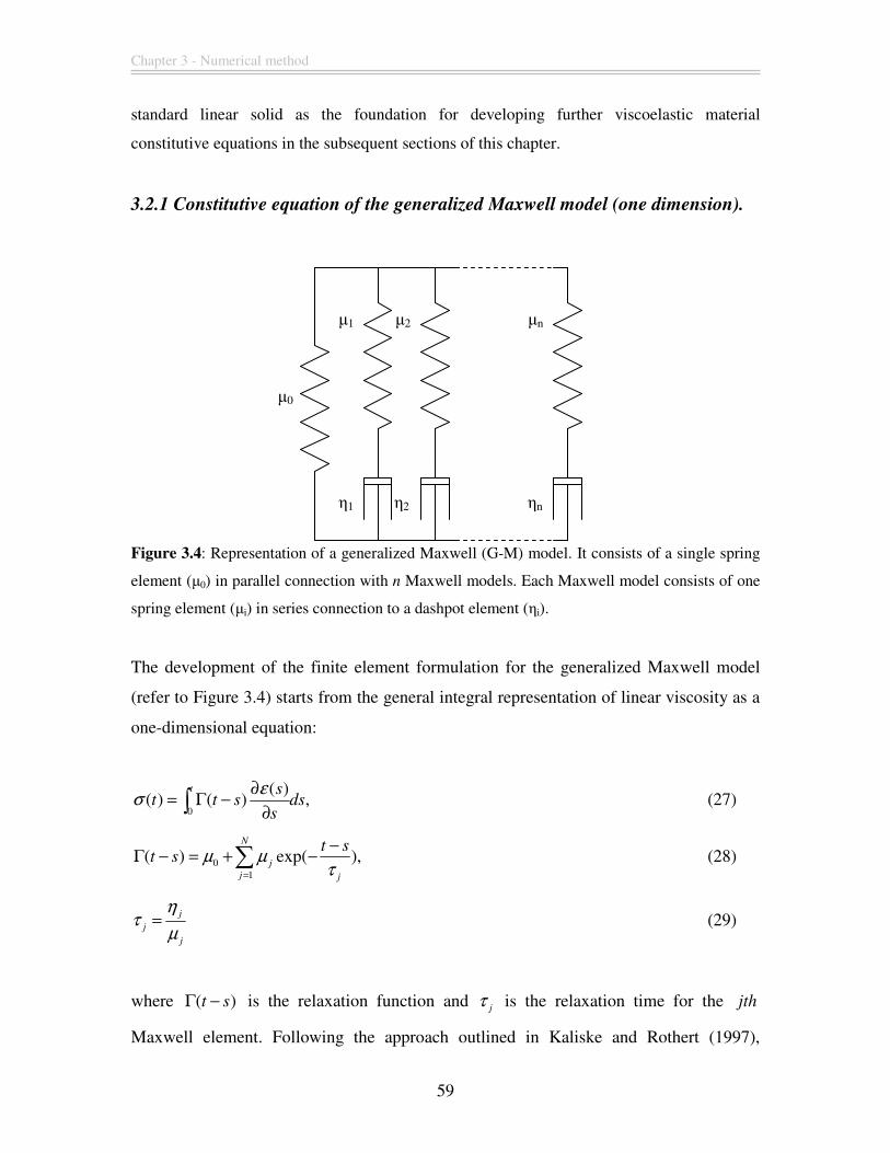
Chapter 3 - Numerical method
59
standard linear solid as the foundation for developing further viscoelastic material
constitutive equations in the subsequent sections of this chapter.
3.2.1 Constitutive equation of the generalized Maxwell model (one dimension).
Figure 3.4: Representation of a generalized Maxwell (G-M) model. It consists of a single spring
element (µ0) in parallel connection with n Maxwell models. Each Maxwell model consists of one
spring element (µi) in series connection to a dashpot element (ηi).
The development of the finite element formulation for the generalized Maxwell model
(refer to Figure 3.4) starts from the general integral representation of linear viscosity as a
one-dimensional equation:
0
( )( ) ( ) ,
t st t s ds
s
εσ
∂= Γ −
∂∫ (27)
01
( ) exp( ),N
j
j j
t st s µ µ
τ=
−Γ − = + −∑ (28)
j
j
j
ητ
µ= (29)
where ( )t sΓ − is the relaxation function and j
τ is the relaxation time for the jth
Maxwell element. Following the approach outlined in Kaliske and Rothert (1997),
µ0
µ1 µ2 µn
η1 η2 ηn
Chapter 3 - Numerical method
60
splitting the integral into an elastic and a viscoelastic contribution leads to the elastic
stress component 0 ( )tσ and the internal stress equivalent variable ( )j
h t as shown:
00 01
( ) ( )( ) exp( )
Nt t
j
j j
s t s st ds ds
s s
ε εσ µ µ
τ=
∂ − ∂= + −
∂ ∂∑∫ ∫ (30)
0 01
( )( ) exp( )
Nt
j
j j
t s st ds
s
εµ ε µ
τ=
− ∂= + −
∂∑∫ (31)
01
( ) ( ).N
j
j
t h tσ=
= +∑ (32)
The internal stress equivalent variable ( )j
h t can be evaluated using the recursive formula
given by Kaliske and Rothert (1997):
1 10 0
1 exp( )
( ) exp( ) [ ],jn n n n
j j j
j
j
t
th t h
t
τγ σ σ
ττ
+ +
∆− −
∆= − + −
∆ (33)
0
.j
j
µγ
µ= (34)
This recursive determination of the current 1n
jh+ requires the quantities 0
nσ , n
jh where
1,...,j N= of the preceding time step n and, therefore they have to be stored in a data
base. The shown strain-driven integration algorithm is unconditionally stable for small
and large time steps and it is second order accurate.
3.2.2 Constitutive equation of the generalized Maxwell model for multi-axial
stress states
The extension of Equation (32) to a fully two-dimensional or three-dimensional approach
is easily performed by introducing tensor quantities. In a multi-axial stress state, the total
Chapter 3 - Numerical method
61
stress tensor 1n+σ for a linear elastic Maxwell material is determined from the elastic
contribution 10
n+σ and from the internal stress variables 1
jn+
h , where the superscript
represent a specific instant of time 1n + . Thus, we can write the stress tensor 1n+σ in a
multi-axial stress state as follows:
N1 1 1
0 jj 1
,n n n+ + +
=
= +∑σ σ h (35)
1 10 ,n E n+ +=σ D ε (36)
j1 1j j j 0 0
j
j
1 exp( )
exp( ) [ ]n n n n
t
t
t
τγ
ττ
+ +
∆− −
∆= − + −
∆h h σ σ (37)
where ED is the 4th order tensor that is analogous to the elastic spring constant 0µ in the
one-dimensional case.
3.2.3 Finite element formulation
The governing equation of motion for the dynamic deformation of a two-dimensional
solid under plain strain condition at a specific instant of time t is:
ext( ) ( ) ( )t T t t
VdV+ =∫M u B σ f&& (38)
where M is the mass matrix, B is the strain-displacement matrix, extf is the external
load and u is the nodal displacement vector. Substituting Equation (35) into Equation
(38) and making use of Equation (36), we have:
ext0
1
( ) ( ) ( ) ( ) .N
t T t T t t
jV V
j
dV dV=
+ + =∑∫ ∫M u B σ B h f&& (39)
Chapter 3 - Numerical method
62
The standard linear solid (SLS) model consisting of a spring in parallel connection with a
single Maxwell element is a special case of the generalized Maxwell model. For the SLS
model, the upper limit of the summation in the above equation is set to 1N = and
Equation (39) reduces to:
ext0 1( ) ( ) ( ) ( ) ,t T t T t t
V VdV dV+ + =∫ ∫M u B σ B h f&& (40)
1 1 ext1 1 2( ) ( ) { ( ) [( ) ( ) ]} ( )t T E t T t T E t t t
V VdV a a dV
− −⇒ + + + − =∫ ∫M u B D ε B h B D ε ε f&& (41)
where
1
1
exp( )t
aτ
∆= − and 1
2 1
1
1 exp( )
.
t
at
τγ
τ
∆− −
=∆
(42)
Using a constant-strain triangle in our finite element formulation, Equation (41) can be
further simplified as follows:
1 1 ext1 1 2( ) [ ]( ) [ ( ) ] [ ( )] ( )t T E t T t T E t t t
n n nt A a t A a t A
− −+ + + − =M u B D B u B h B D B u u f&&1442443 1444444442444444443
(43)
where n
t and A are the thickness and area of the constant-strain triangle respectively.
3.2.4 Non-dimensionalization
In order to non-dimensionalize Equation (43), we will introduce the following
dimensionless variables u% , t% and M% . The following equations below relate these
dimensionless variables to the actual physical quantities:
0u=u u% , 0t t t= % , 0m=M M% (44)
elastic contribution viscous contribution
Chapter 3 - Numerical method
63
where 0u is the characteristic length scale with dimension of length, 0t is the
characteristic time scale with dimension of time, 0m is the characteristic mass scale with
dimension of mass. We also introduce the characteristic force scale 20Eu , which is the
product of the elastic modulus with the square of the length scale and has the unit of
Newton ( N ). This term will be used to non-dimensionalize the second to fourth
components of Equation (43). Expressing Equation (43) in terms of the dimensionless
variables in Equation (44) and the characteristic force scale, we obtain:
22 2 10 0
0 1 0 12 20
2 1 ext2 0
[ ]( ) [ ( ) ]
[ ( )] ( )
T E t T t
n n
T E t t t
n
m u dEu t A a Eu t A
t dt
a Eu t A
−
−
+ +
+ − =
uM B D B u B h
B D B u u f
% % %% % % % %% %%%
%% % % % %
(45)
where the tilde denotes the dimensionless variables. Normalizing Equation (45) with
respect to the characteristic force scale 20Eu such that the internal forces are of
magnitude O(1), we obtain:
210
1 12 20 0
ext1
2 20
[ ]( ) [ ( ) ]
( )[ ( )] .
T E t T t
n n
tT E t t
n
m dt A a t A
Eu t dt
a t AEu
−
−
+ +
+ − =
uM B D B u B h
fB D B u u
% % %% % % % %% %%%
%% % % % %
(46)
Using the values of the physical constants reported in Thoumine and Ott (1997a) for the
microplate manipulation of fibroblasts, we can obtain estimates for the following:
a. Elastic modulus, E=0µ ≈ 9.6 x 10² 2/ mN ,
b. Elastic modulus for Maxwell element, 1µ ≈ 5.1 x 10² 2/ mN ,
c. Viscosity for Maxwell element, 1η ≈ 1.3 x 10⁴ Pas ,
d. Density ρ = 1000 3/ mkg ,
e. Characteristic length scale 60 5*10u m
−= ,
Chapter 3 - Numerical method
64
f. Characteristic time scale 0 1t s= .
Using these values, we can obtain estimates for 0m and the dimensionless density ρ~
used to compute the consistent mass matrix in Equation (11):
3 6 3 130 0 1000*(5*10 ) 1.25*10 ,m u kgρ − −= = = (47)
13110
2 2 6 20 0
1.25*102.6*10 .
(9.6*10 )*(5*10 )*(1)
m
Eu tρ
−−
−⇒ = = ≈% (48)
We can see that the inertia term is several orders of magnitude smaller compared to the
internal force terms and we can neglect its effect which is equivalent to using a
dimensionless density 0~ =ρ in our finite element simulation. For the external forcing
term extf , we can see that it is being normalized with respect to the characteristic force
scale 20Eu .
ext ext extext
2 2 6 2 90
( ) ( ) ( )( ) .
(9.6*10 )*(5*10 ) 24*10
t t tt
Eu− −
⇒ = = =f f f
f% (49)
This gives us an estimation that if the external load applied to the system is in the region
of a few nano-Newtons ( nN ), the non-dimensional external load term ext( )tf% will be of
magnitude O(1) also which is comparable to the internal force terms. Using the material
properties reported in Thoumine and Ott (1997a) and scaling them with the characteristic
force scale 20Eu , the following dimensionless parameters to be used for our finite
element simulation are obtained:
a. Dimensionless elastic modulus, 0 Eµ = %% = 1,
b. Dimensionless elastic modulus for Maxwell element, 1µ% = 0.53,
c. Dimensionless viscosity for Maxwell element, 1η% = 13.5,
d. Dimensionless density ρ% = 0 .
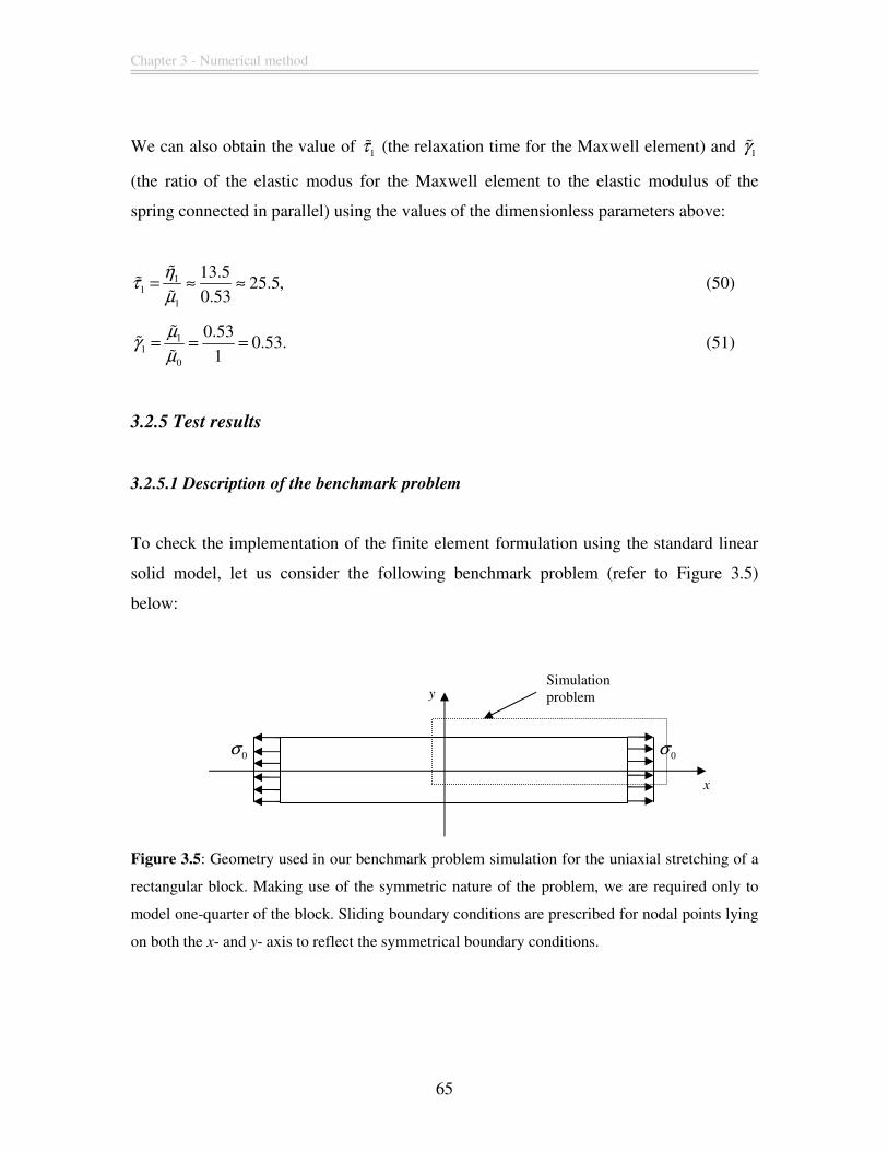
Chapter 3 - Numerical method
65
We can also obtain the value of 1τ% (the relaxation time for the Maxwell element) and 1γ%
(the ratio of the elastic modus for the Maxwell element to the elastic modulus of the
spring connected in parallel) using the values of the dimensionless parameters above:
11
1
13.525.5,
0.53
ητ
µ= ≈ ≈
%%
% (50)
11
0
0.530.53.
1
µγ
µ= = =
%%
% (51)
3.2.5 Test results
3.2.5.1 Description of the benchmark problem
To check the implementation of the finite element formulation using the standard linear
solid model, let us consider the following benchmark problem (refer to Figure 3.5)
below:
Figure 3.5: Geometry used in our benchmark problem simulation for the uniaxial stretching of a
rectangular block. Making use of the symmetric nature of the problem, we are required only to
model one-quarter of the block. Sliding boundary conditions are prescribed for nodal points lying
on both the x- and y- axis to reflect the symmetrical boundary conditions.
0σ 0σ
x
y Simulation problem
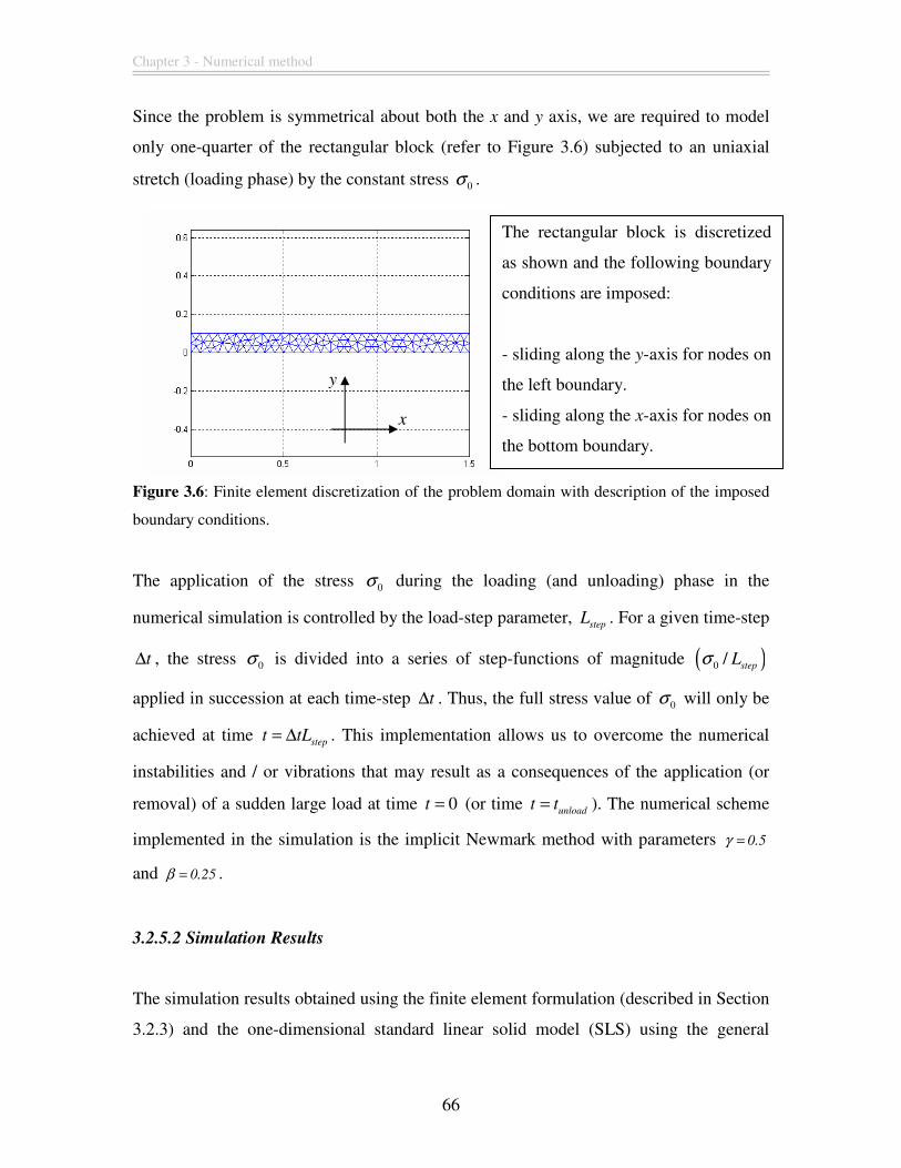
Chapter 3 - Numerical method
66
Since the problem is symmetrical about both the x and y axis, we are required to model
only one-quarter of the rectangular block (refer to Figure 3.6) subjected to an uniaxial
stretch (loading phase) by the constant stress 0σ .
Figure 3.6: Finite element discretization of the problem domain with description of the imposed
boundary conditions.
The application of the stress 0σ during the loading (and unloading) phase in the
numerical simulation is controlled by the load-step parameter, step
L . For a given time-step
t∆ , the stress 0σ is divided into a series of step-functions of magnitude ( )0 /step
Lσ
applied in succession at each time-step t∆ . Thus, the full stress value of 0σ will only be
achieved at time step
t tL= ∆ . This implementation allows us to overcome the numerical
instabilities and / or vibrations that may result as a consequences of the application (or
removal) of a sudden large load at time 0t = (or time unload
t t= ). The numerical scheme
implemented in the simulation is the implicit Newmark method with parameters 0.5γ =
and 0.25β = .
3.2.5.2 Simulation Results
The simulation results obtained using the finite element formulation (described in Section
3.2.3) and the one-dimensional standard linear solid model (SLS) using the general
The rectangular block is discretized
as shown and the following boundary
conditions are imposed:
- sliding along the y-axis for nodes on
the left boundary.
- sliding along the x-axis for nodes on
the bottom boundary.
x
y
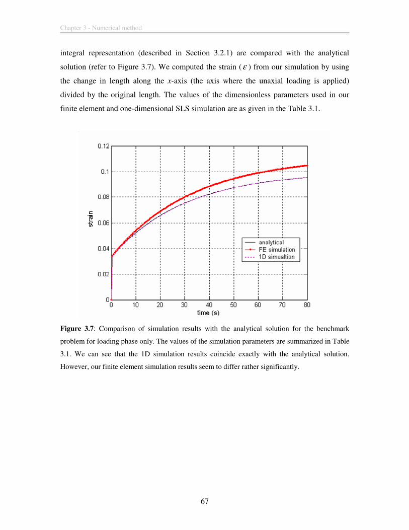
Chapter 3 - Numerical method
67
integral representation (described in Section 3.2.1) are compared with the analytical
solution (refer to Figure 3.7). We computed the strain (ε ) from our simulation by using
the change in length along the x-axis (the axis where the unaxial loading is applied)
divided by the original length. The values of the dimensionless parameters used in our
finite element and one-dimensional SLS simulation are as given in the Table 3.1.
Figure 3.7: Comparison of simulation results with the analytical solution for the benchmark
problem for loading phase only. The values of the simulation parameters are summarized in Table
3.1. We can see that the 1D simulation results coincide exactly with the analytical solution.
However, our finite element simulation results seem to differ rather significantly.
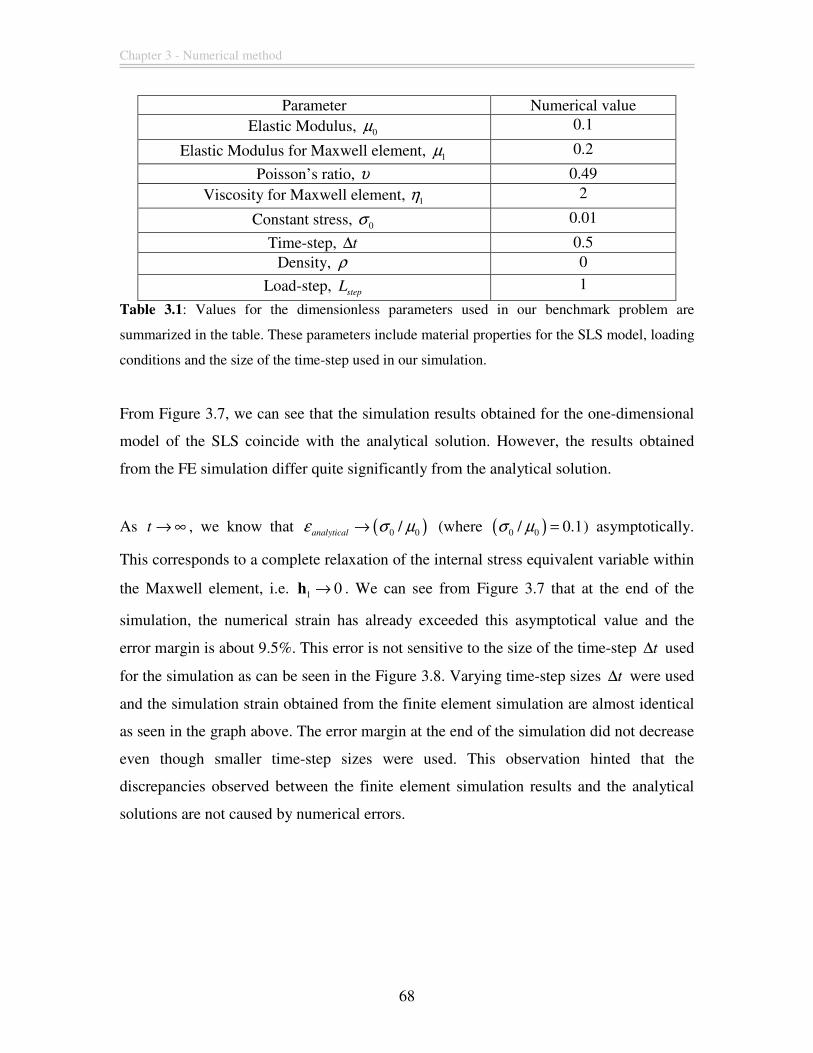
Chapter 3 - Numerical method
68
Parameter Numerical value Elastic Modulus, 0µ 0.1
Elastic Modulus for Maxwell element, 1µ 0.2
Poisson’s ratio, υ 0.49
Viscosity for Maxwell element, 1η 2
Constant stress, 0σ 0.01
Time-step, t∆ 0.5 Density, ρ 0
Load-step, step
L 1
Table 3.1: Values for the dimensionless parameters used in our benchmark problem are
summarized in the table. These parameters include material properties for the SLS model, loading
conditions and the size of the time-step used in our simulation.
From Figure 3.7, we can see that the simulation results obtained for the one-dimensional
model of the SLS coincide with the analytical solution. However, the results obtained
from the FE simulation differ quite significantly from the analytical solution.
As t → ∞ , we know that ( )0 0/analyticalε σ µ→ (where ( )0 0/ 0.1σ µ = ) asymptotically.
This corresponds to a complete relaxation of the internal stress equivalent variable within
the Maxwell element, i.e. 1 0→h . We can see from Figure 3.7 that at the end of the
simulation, the numerical strain has already exceeded this asymptotical value and the
error margin is about 9.5%. This error is not sensitive to the size of the time-step t∆ used
for the simulation as can be seen in the Figure 3.8. Varying time-step sizes t∆ were used
and the simulation strain obtained from the finite element simulation are almost identical
as seen in the graph above. The error margin at the end of the simulation did not decrease
even though smaller time-step sizes were used. This observation hinted that the
discrepancies observed between the finite element simulation results and the analytical
solutions are not caused by numerical errors.
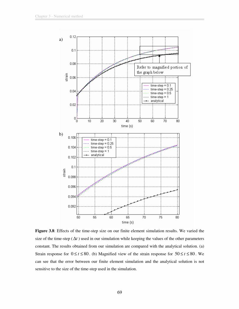
Chapter 3 - Numerical method
69
Figure 3.8: Effects of the time-step size on our finite element simulation results. We varied the
size of the time-step ( t∆ ) used in our simulation while keeping the values of the other parameters
constant. The results obtained from our simulation are compared with the analytical solution. (a)
Strain response for 0 80t≤ ≤ . (b) Magnified view of the strain response for 50 80t≤ ≤ . We
can see that the error between our finite element simulation and the analytical solution is not
sensitive to the size of the time-step used in the simulation.
a)
b)
Chapter 3 - Numerical method
70
We note that the analytical solutions obtained from solving the governing one-
dimensional differential equation for the SLS model is an idealization. The spring
constants, 0µ and 1µ , are constant and hence, the system has a constant stiffness
independent of the strain. However, the stiffness of the rectangular block in the finite
element simulation is updated at every time-step based on its deformed configuration in a
“pseudo-updated Lagrangian” approach. This means that the stiffness of the system in the
finite element simulation is time dependent even though the material properties such as
the two elastic moduli and viscosity are time-independent. This difference is also noted in
the stress applied to the system in the analytical scenario and the finite element
simulation. In the analytical case, the stress is equivalent to the force applied to the
system because the cross-sectional area is taken as unity, thus the applied force is time-
independent. However, this is not applicable for the finite element simulation. In the
finite element simulation, the force is obtained by multiplying the stress by the cross-
sectional area of the rectangular block. Since the cross-sectional area varies with the
deformation of the rectangular block, we can see that the force applied to the system in
the finite element simulation is time-dependent. Let us consider the following correction
to the finite element simulation to account for the time-independent characteristics of the
one-dimensional analytical system of the SLS.
Starting from the linear relationship between stress ( )tσ and strain ( )tε , we have:
( ) ( ) / ( ) ( ) ( )t F t S t K t tσ ε= = (52)
where ( )F t is the force applied to the system at time t , ( )S t is the cross-sectional area
of the system at time t and ( )K t is the effective stiffness of the system at time t taking
into account both the elastic and viscous component. Let us assume that the effective
stiffness ( )K t at time t is related to the initial stiffness of the system which is denoted by
0K by the following equation:
0 0( ) ( ) /K t K S t S= (53)
Chapter 3 - Numerical method
71
where 0S is the initial cross-sectional area of the system. Substituting Equation (53) into
Equation (52), we obtain:
0 0 0 0( ) ( ) / ( ( ) / )( / ( )),K S t t S F t S S S tε = (54)
20 0 0( ) ( ( ) / )(1/ )( / ( )) .t F t S K S S tε = (55)
In order to correct the finite element simulation to the idealized one-dimensional
analytical solution, let us denote the time-dependent force ( )F t in the finite element
simulation with the equation:
20 0( ) ( ( ) / )F t F S t S= (56)
where 0F is the initial force applied to the system. The corrected simulation result for the
finite element formulation is compared against the simulation results obtained for the
one-dimensional model of the SLS and the analytical solution (refer to Figure 3.9). We
can see that the corrected finite element results are in excellent agreement with the
analytical solution. This further confirms that the initial discrepancies between the finite
element simulation and the analytical solution arise owing to the different characteristics
and assumptions made in the two systems considered. Thus, it can be seen that the
general integral representation can be used successfully to model the linear viscoelastic
constitutive equation of the SLS mechanical model within a finite element formulation
framework.
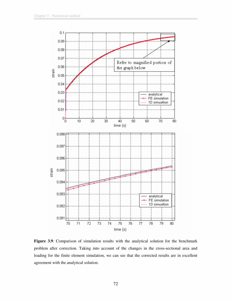
Chapter 3 - Numerical method
72
Figure 3.9: Comparison of simulation results with the analytical solution for the benchmark
problem after correction. Taking into account of the changes in the cross-sectional area and
loading for the finite element simulation, we can see that the corrected results are in excellent
agreement with the analytical solution.
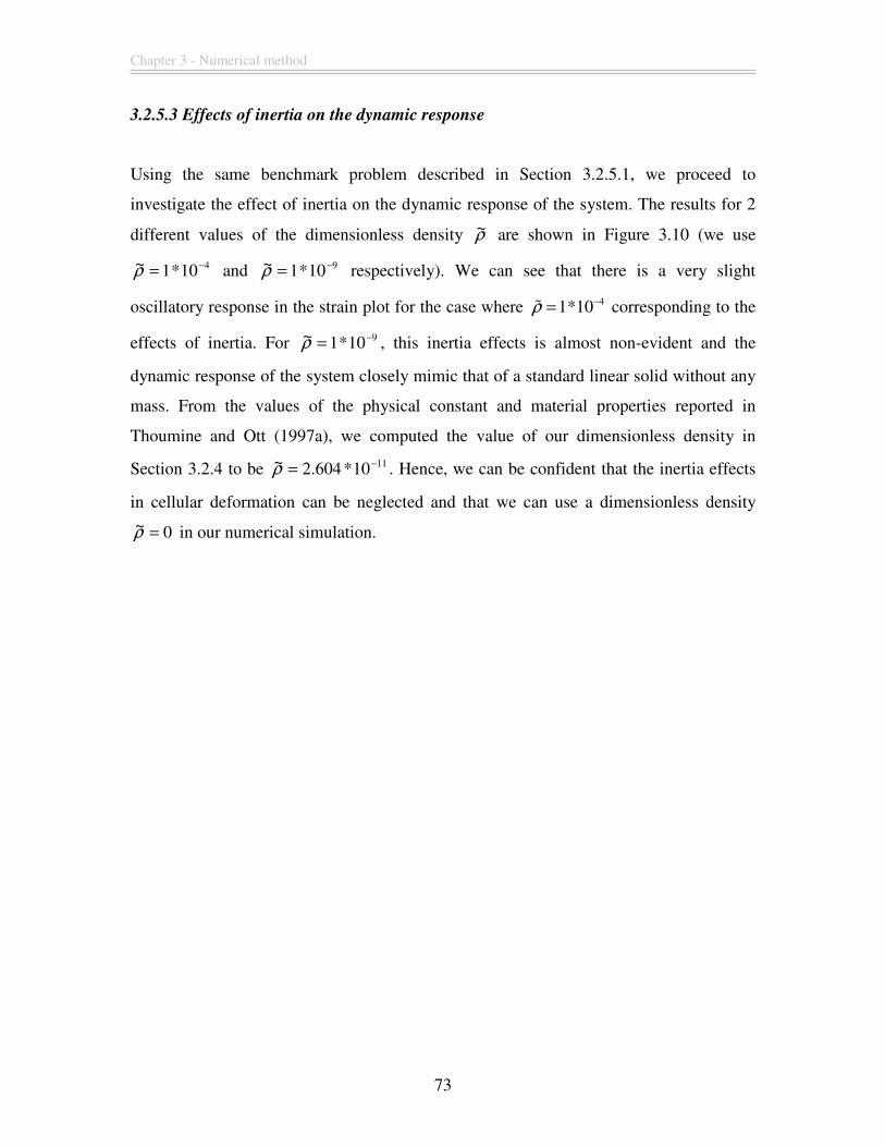
Chapter 3 - Numerical method
73
3.2.5.3 Effects of inertia on the dynamic response
Using the same benchmark problem described in Section 3.2.5.1, we proceed to
investigate the effect of inertia on the dynamic response of the system. The results for 2
different values of the dimensionless density ρ~ are shown in Figure 3.10 (we use
410*1~ −=ρ and 910*1~ −=ρ respectively). We can see that there is a very slight
oscillatory response in the strain plot for the case where 41*10ρ −=% corresponding to the
effects of inertia. For 910*1~ −=ρ , this inertia effects is almost non-evident and the
dynamic response of the system closely mimic that of a standard linear solid without any
mass. From the values of the physical constant and material properties reported in
Thoumine and Ott (1997a), we computed the value of our dimensionless density in
Section 3.2.4 to be 1110*604.2~ −=ρ . Hence, we can be confident that the inertia effects
in cellular deformation can be neglected and that we can use a dimensionless density
0~ =ρ in our numerical simulation.
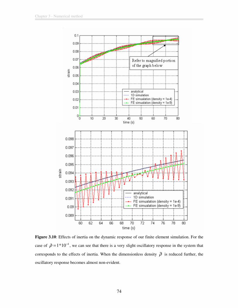
Chapter 3 - Numerical method
74
Figure 3.10: Effects of inertia on the dynamic response of our finite element simulation. For the
case of 41*10ρ −=% , we can see that there is a very slight oscillatory response in the system that
corresponds to the effects of inertia. When the dimensionless density ρ~ is reduced further, the
oscillatory response becomes almost non-evident.
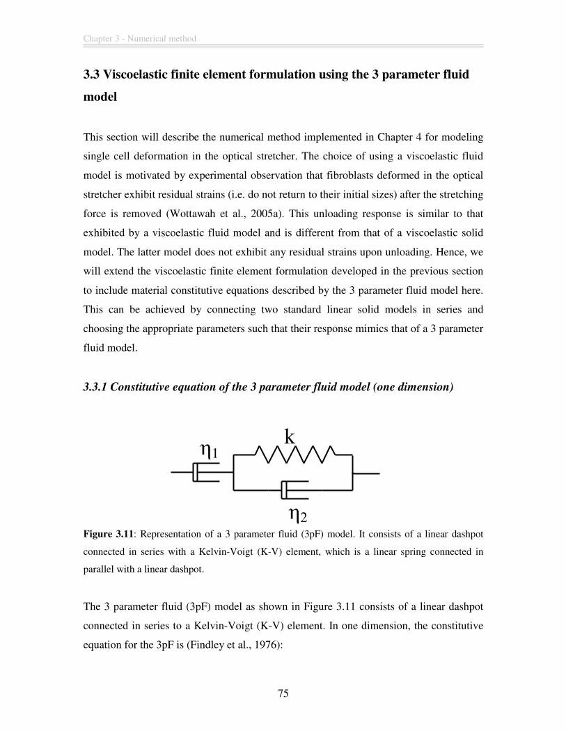
Chapter 3 - Numerical method
75
3.3 Viscoelastic finite element formulation using the 3 parameter fluid
model
This section will describe the numerical method implemented in Chapter 4 for modeling
single cell deformation in the optical stretcher. The choice of using a viscoelastic fluid
model is motivated by experimental observation that fibroblasts deformed in the optical
stretcher exhibit residual strains (i.e. do not return to their initial sizes) after the stretching
force is removed (Wottawah et al., 2005a). This unloading response is similar to that
exhibited by a viscoelastic fluid model and is different from that of a viscoelastic solid
model. The latter model does not exhibit any residual strains upon unloading. Hence, we
will extend the viscoelastic finite element formulation developed in the previous section
to include material constitutive equations described by the 3 parameter fluid model here.
This can be achieved by connecting two standard linear solid models in series and
choosing the appropriate parameters such that their response mimics that of a 3 parameter
fluid model.
3.3.1 Constitutive equation of the 3 parameter fluid model (one dimension)
Figure 3.11: Representation of a 3 parameter fluid (3pF) model. It consists of a linear dashpot
connected in series with a Kelvin-Voigt (K-V) element, which is a linear spring connected in
parallel with a linear dashpot.
The 3 parameter fluid (3pF) model as shown in Figure 3.11 consists of a linear dashpot
connected in series to a Kelvin-Voigt (K-V) element. In one dimension, the constitutive
equation for the 3pF is (Findley et al., 1976):
k η1
η2
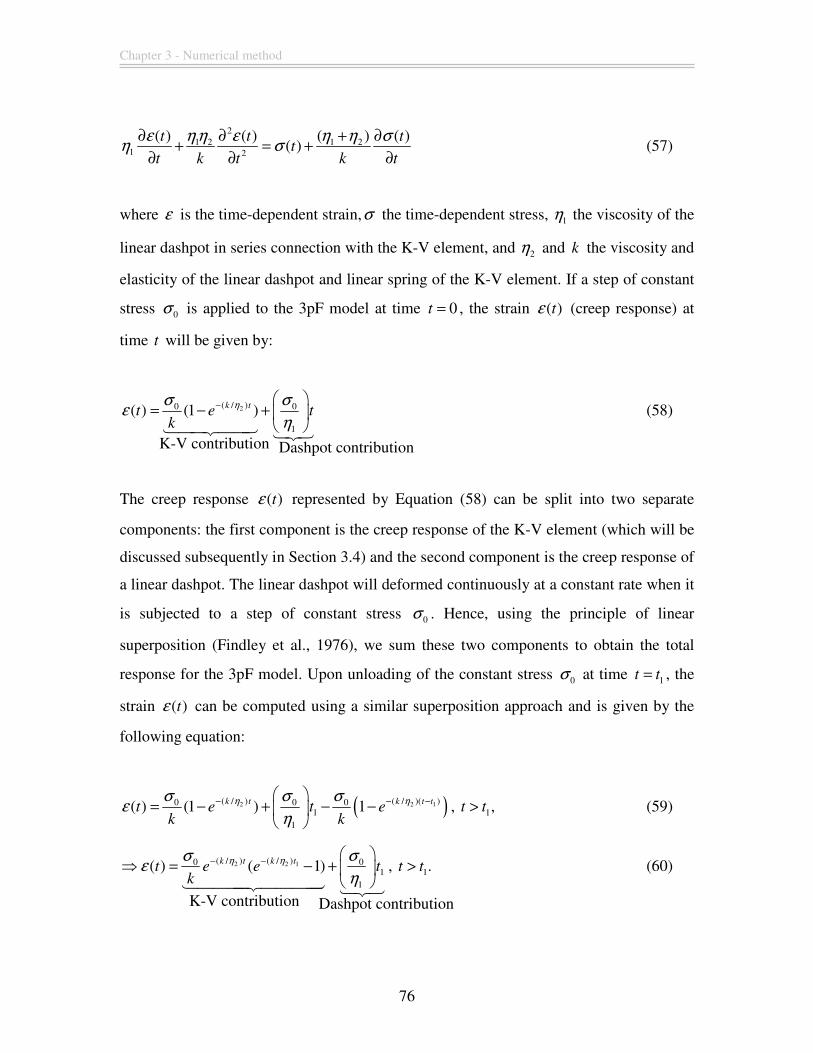
Chapter 3 - Numerical method
76
21 2 1 2
1 2
( )( ) ( ) ( )( )
t t tt
t k t k t
η η η ηε ε ση σ
+∂ ∂ ∂+ = +
∂ ∂ ∂ (57)
where ε is the time-dependent strain,σ the time-dependent stress, 1η the viscosity of the
linear dashpot in series connection with the K-V element, and 2η and k the viscosity and
elasticity of the linear dashpot and linear spring of the K-V element. If a step of constant
stress 0σ is applied to the 3pF model at time 0t = , the strain ( )tε (creep response) at
time t will be given by:
2( / )0 0
1
( ) (1 )k tt e t
k
ησ σε
η−
= − + 1442443 123
(58)
The creep response ( )tε represented by Equation (58) can be split into two separate
components: the first component is the creep response of the K-V element (which will be
discussed subsequently in Section 3.4) and the second component is the creep response of
a linear dashpot. The linear dashpot will deformed continuously at a constant rate when it
is subjected to a step of constant stress 0σ . Hence, using the principle of linear
superposition (Findley et al., 1976), we sum these two components to obtain the total
response for the 3pF model. Upon unloading of the constant stress 0σ at time 1t t= , the
strain ( )tε can be computed using a similar superposition approach and is given by the
following equation:
( )2 2 1( / ) ( / )( )0 0 01
1
( ) (1 ) 1k t k t tt e t e
k k
η ησ σ σε
η− − −
= − + − −
, 1,t t> (59)
2 2 1( / ) ( / )0 01
1
( ) ( 1)k t k tt e e t
k
η ησ σε
η− −
⇒ = − + 14444244443 123
, 1.t t> (60)
K-V contribution Dashpot contribution
K-V contribution Dashpot contribution
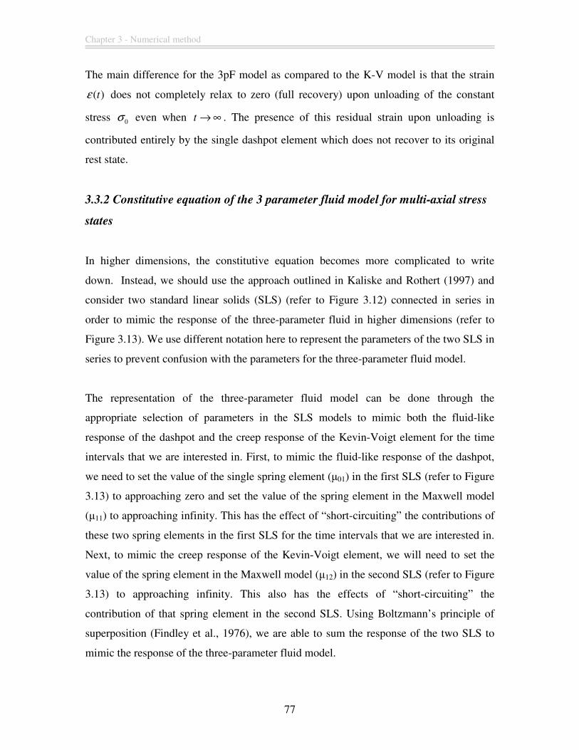
Chapter 3 - Numerical method
77
The main difference for the 3pF model as compared to the K-V model is that the strain
( )tε does not completely relax to zero (full recovery) upon unloading of the constant
stress 0σ even when t → ∞ . The presence of this residual strain upon unloading is
contributed entirely by the single dashpot element which does not recover to its original
rest state.
3.3.2 Constitutive equation of the 3 parameter fluid model for multi-axial stress
states
In higher dimensions, the constitutive equation becomes more complicated to write
down. Instead, we should use the approach outlined in Kaliske and Rothert (1997) and
consider two standard linear solids (SLS) (refer to Figure 3.12) connected in series in
order to mimic the response of the three-parameter fluid in higher dimensions (refer to
Figure 3.13). We use different notation here to represent the parameters of the two SLS in
series to prevent confusion with the parameters for the three-parameter fluid model.
The representation of the three-parameter fluid model can be done through the
appropriate selection of parameters in the SLS models to mimic both the fluid-like
response of the dashpot and the creep response of the Kevin-Voigt element for the time
intervals that we are interested in. First, to mimic the fluid-like response of the dashpot,
we need to set the value of the single spring element (µ01) in the first SLS (refer to Figure
3.13) to approaching zero and set the value of the spring element in the Maxwell model
(µ11) to approaching infinity. This has the effect of “short-circuiting” the contributions of
these two spring elements in the first SLS for the time intervals that we are interested in.
Next, to mimic the creep response of the Kevin-Voigt element, we will need to set the
value of the spring element in the Maxwell model (µ12) in the second SLS (refer to Figure
3.13) to approaching infinity. This also has the effects of “short-circuiting” the
contribution of that spring element in the second SLS. Using Boltzmann’s principle of
superposition (Findley et al., 1976), we are able to sum the response of the two SLS to
mimic the response of the three-parameter fluid model.
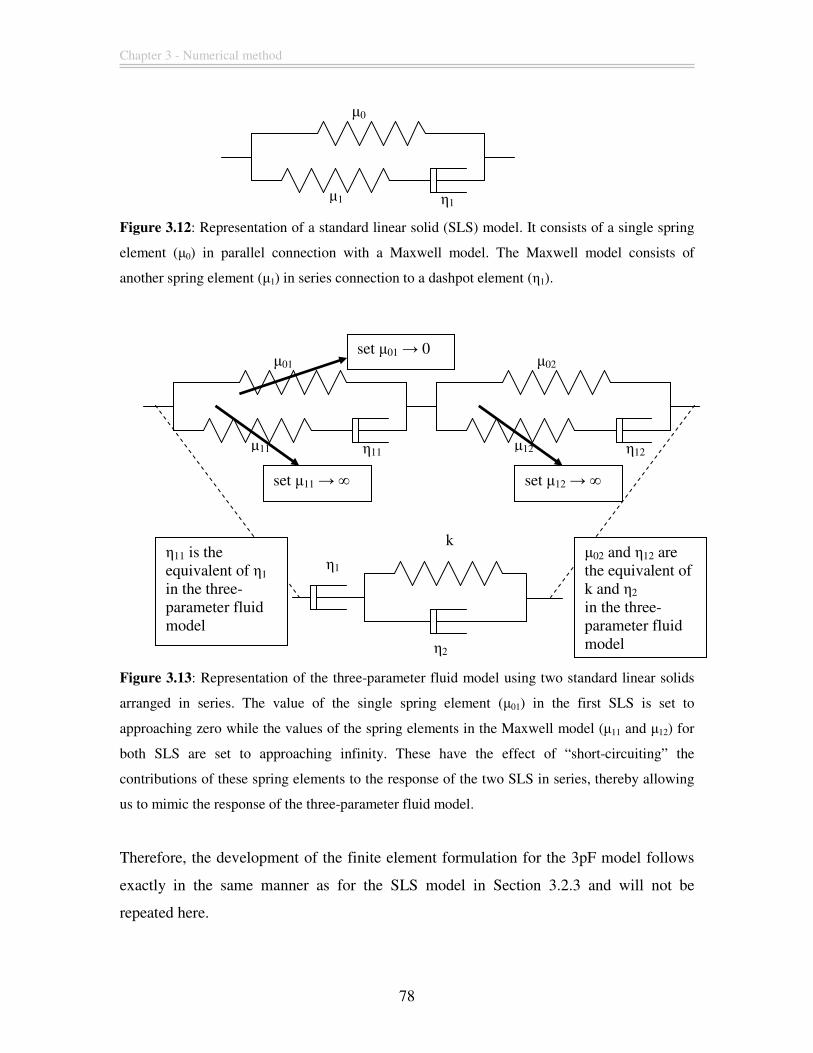
Chapter 3 - Numerical method
78
Figure 3.12: Representation of a standard linear solid (SLS) model. It consists of a single spring
element (µ0) in parallel connection with a Maxwell model. The Maxwell model consists of
another spring element (µ1) in series connection to a dashpot element (η1).
Figure 3.13: Representation of the three-parameter fluid model using two standard linear solids
arranged in series. The value of the single spring element (µ01) in the first SLS is set to
approaching zero while the values of the spring elements in the Maxwell model (µ11 and µ12) for
both SLS are set to approaching infinity. These have the effect of “short-circuiting” the
contributions of these spring elements to the response of the two SLS in series, thereby allowing
us to mimic the response of the three-parameter fluid model.
Therefore, the development of the finite element formulation for the 3pF model follows
exactly in the same manner as for the SLS model in Section 3.2.3 and will not be
repeated here.
µ0
µ1 η1
µ01
µ11 η11
µ02
µ12 η12
set µ12 → ∞
set µ11 → ∞
set µ01 → 0
k
η1
η2
η11 is the equivalent of η1
in the three-parameter fluid model
µ02 and η12 are the equivalent of k and η2
in the three-parameter fluid model
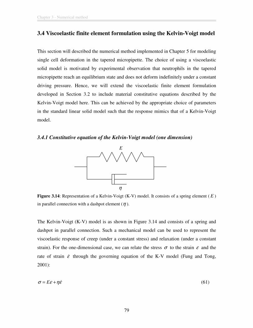
Chapter 3 - Numerical method
79
3.4 Viscoelastic finite element formulation using the Kelvin-Voigt model
This section will described the numerical method implemented in Chapter 5 for modeling
single cell deformation in the tapered micropipette. The choice of using a viscoelastic
solid model is motivated by experimental observation that neutrophils in the tapered
micropipette reach an equilibrium state and does not deform indefinitely under a constant
driving pressure. Hence, we will extend the viscoelastic finite element formulation
developed in Section 3.2 to include material constitutive equations described by the
Kelvin-Voigt model here. This can be achieved by the appropriate choice of parameters
in the standard linear solid model such that the response mimics that of a Kelvin-Voigt
model.
3.4.1 Constitutive equation of the Kelvin-Voigt model (one dimension)
Figure 3.14: Representation of a Kelvin-Voigt (K-V) model. It consists of a spring element ( E )
in parallel connection with a dashpot element (η ).
The Kelvin-Voigt (K-V) model is as shown in Figure 3.14 and consists of a spring and
dashpot in parallel connection. Such a mechanical model can be used to represent the
viscoelastic response of creep (under a constant stress) and relaxation (under a constant
strain). For the one-dimensional case, we can relate the stress σ to the strain ε and the
rate of strain ε& through the governing equation of the K-V model (Fung and Tong,
2001):
Eσ ε ηε= + & (61)
E
η
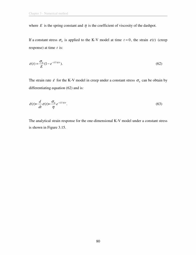
Chapter 3 - Numerical method
80
where E is the spring constant and η is the coefficient of viscosity of the dashpot.
If a constant stress 0σ is applied to the K-V model at time 0t = , the strain ( )tε (creep
response) at time t is:
( / )0( ) (1 ).E tt e
E
ησε −= − (62)
The strain rate ε& for the K-V model in creep under a constant stress 0σ can be obtain by
differentiating equation (62) and is:
( / )0( ) ( ) .E tdt t e
dt
ησε ε
η−= =& (63)
The analytical strain response for the one-dimensional K-V model under a constant stress
is shown in Figure 3.15.
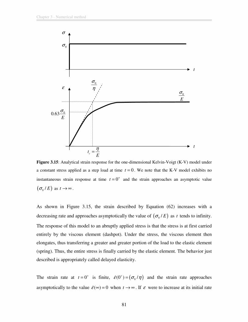
Chapter 3 - Numerical method
81
Figure 3.15: Analytical strain response for the one-dimensional Kelvin-Voigt (K-V) model under
a constant stress applied as a step load at time 0t = . We note that the K-V model exhibits no
instantaneous strain response at time 0t+= and the strain approaches an asymptotic value
( )0 / Eσ as t → ∞ .
As shown in Figure 3.15, the strain described by Equation (62) increases with a
decreasing rate and approaches asymptotically the value of ( )0 / Eσ as t tends to infinity.
The response of this model to an abruptly applied stress is that the stress is at first carried
entirely by the viscous element (dashpot). Under the stress, the viscous element then
elongates, thus transferring a greater and greater portion of the load to the elastic element
(spring). Thus, the entire stress is finally carried by the elastic element. The behavior just
described is appropriately called delayed elasticity.
The strain rate at 0t+= is finite, ( )0(0 ) /ε σ η+ =& and the strain rate approaches
asymptotically to the value ( ) 0ε ∞ =& when t → ∞ . If ε were to increase at its initial rate
0σ
σ
t
t
ε
0
E
σ
ct
E
η=
00.63E
σ
0σ
η
Chapter 3 - Numerical method
82
( )0 /σ η , it would cross the asymptotic value ( )0 / Eσ at c
t t= where c
t is known as the
retardation time. At c
t t= ,
10 0(1 ) 0.63 .eE E
σ σε −= − = (64)
Thus, only 37% of the asymptotic strain remains to be accomplished after c
t t= . If the
stress is removed at 1t t= , the strain following stress removal can be determined by the
superposition principle. The strain ( )a
tε in the K-V model resulting from stress 0σ
applied at time 0t = is:
( / )0( ) (1 ).E t
at e
E
ησε −= − (65)
The strain ( )b
tε resulting from applying a stress 0( )σ− independently at time 1t t= is:
1( / )( )0( ) [1 ].E t t
bt e
E
ησε − −= − − (66)
If the stress 0σ is applied at 0t = and removed at 1t t= , i.e. 0σ− is applied at 1t t= , the
superposition principle yields the strain ( )tε for 1t t> during recovery:
1( / )( / )0( ) ( ) ( ) ( 1)E tE t
a bt t t e e
E
ηησε ε ε −−= + = − , 1.t t> (67)
When t → ∞ , ( ) 0tε → (full recovery).
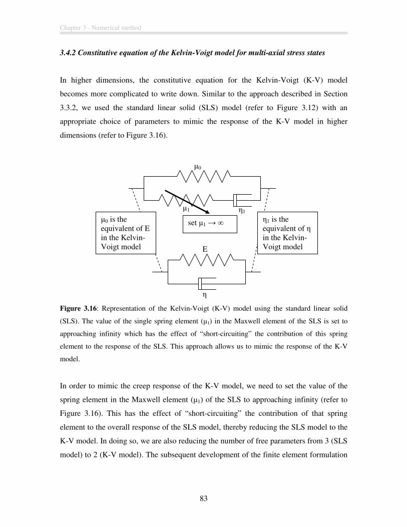
Chapter 3 - Numerical method
83
3.4.2 Constitutive equation of the Kelvin-Voigt model for multi-axial stress states
In higher dimensions, the constitutive equation for the Kelvin-Voigt (K-V) model
becomes more complicated to write down. Similar to the approach described in Section
3.3.2, we used the standard linear solid (SLS) model (refer to Figure 3.12) with an
appropriate choice of parameters to mimic the response of the K-V model in higher
dimensions (refer to Figure 3.16).
Figure 3.16: Representation of the Kelvin-Voigt (K-V) model using the standard linear solid
(SLS). The value of the single spring element (µ1) in the Maxwell element of the SLS is set to
approaching infinity which has the effect of “short-circuiting” the contribution of this spring
element to the response of the SLS. This approach allows us to mimic the response of the K-V
model.
In order to mimic the creep response of the K-V model, we need to set the value of the
spring element in the Maxwell element (µ1) of the SLS to approaching infinity (refer to
Figure 3.16). This has the effect of “short-circuiting” the contribution of that spring
element to the overall response of the SLS model, thereby reducing the SLS model to the
K-V model. In doing so, we are also reducing the number of free parameters from 3 (SLS
model) to 2 (K-V model). The subsequent development of the finite element formulation
µ0
µ1 η1
set µ1 → ∞
E
η
η1 is the equivalent of η
in the Kelvin-Voigt model
µ0 is the equivalent of E
in the Kelvin-Voigt model
Chapter 3 - Numerical method
84
for the K-V model follows exactly in the same manner as for the SLS model in Section
3.2.3 and will not be repeated here.
3.5 Axisymmetric stress analysis
In this section, we will consider the analysis of stress distribution in axisymmetric solids
(refer to Figure 3.17), defined by the presence of an axis of revolution, under axisymetric
loading. The mathematical formulation presented here are very similar to those of two
dimensional plain strain (refer to Section 3.1) as this problem is also two dimensional. By
symmetry, the two components of any displacement in any plane section of the body
along its axis of symmetry define completely the state of strain and, therefore the state of
stress. Hence, axisymmetric problems in three dimensions can be analyzed in two
dimensions. If r and z denote the radial and axial coordinates of a point respectively, with
u and v being the corresponding displacements, then the same displacement functions
used in section 3.1.3 can be used to define the displacement within the triangular element
i, j, m shown in Figure 3.17. The volume of material associated with a triangular element
is now that of a body of revolution indicated in Figure 3.17 and all integrations have to be
referred to this volume.
In plain strain problems, we noted that the state of strain is completely defined by the
three strain components in the coordinate plane (i.e. xx
ε , yy
ε and xy
ε ). The strain
components normal to this plane are not involved in our analysis due to zero values of
either stress or strain. In the axisymmetrical situation, any radial displacement
automatically induces a strain in the circumferential direction and as the stresses in this
direction are certainly non-zero, this fourth component of strain and of the associated
stress has to the considered. This is the essential differences in the treatment of the
axisymmetrical situation as compared to the plain strain situation.
The algebra involved for axisymmetrical stress analysis will be slightly more tedious than
that in Section 3.1 but essentially identical operations are once again involved, following
the general formulation of Section 3.1.
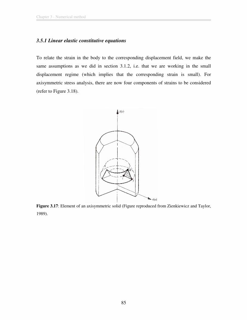
Chapter 3 - Numerical method
85
3.5.1 Linear elastic constitutive equations
To relate the strain in the body to the corresponding displacement field, we make the
same assumptions as we did in section 3.1.2, i.e. that we are working in the small
displacement regime (which implies that the corresponding strain is small). For
axisymmetric stress analysis, there are now four components of strains to be considered
(refer to Figure 3.18).
Figure 3.17: Element of an axisymmetric solid (Figure reproduced from Zienkiewicz and Taylor,
1989).
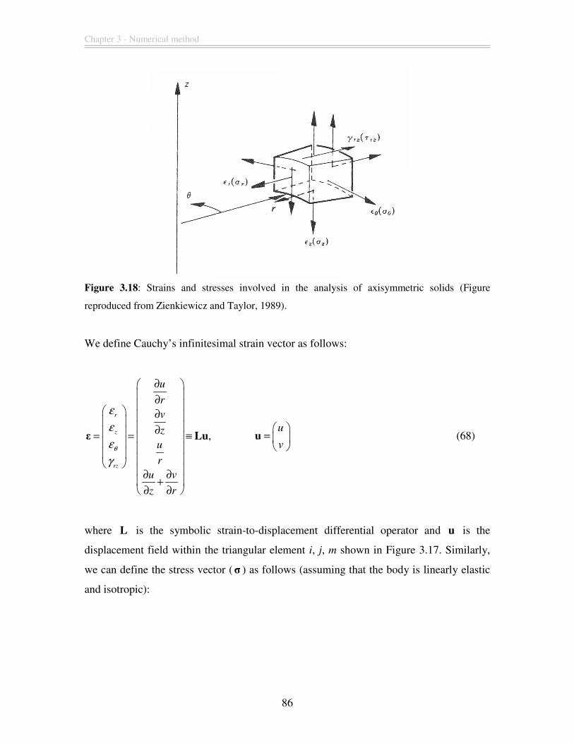
Chapter 3 - Numerical method
86
Figure 3.18: Strains and stresses involved in the analysis of axisymmetric solids (Figure
reproduced from Zienkiewicz and Taylor, 1989).
We define Cauchy’s infinitesimal strain vector as follows:
,
r
z
rz
u
r
v
z
u
r
u v
z r
θ
ε
ε
ε
γ
∂ ∂ ∂ ∂ = = ≡ ∂ ∂ +
∂ ∂
ε Lu u
v
=
u (68)
where L is the symbolic strain-to-displacement differential operator and u is the
displacement field within the triangular element i, j, m shown in Figure 3.17. Similarly,
we can define the stress vector (σ ) as follows (assuming that the body is linearly elastic
and isotropic):
Chapter 3 - Numerical method
87
2 0
2 0
2 0
0 0 0
r r
z z
rz rz
θ θ
σ ελ µ λ λ
σ ελ λ µ λ
σ ελ λ λ µ
τ γµ
+
+ = = +
Dε (69)
where D is the elastic modulus tensor, λ and µ are Lame’s constants defined in exactly
the same manner as for plain strain problems in Equation (6).
Using linear triangle elements for the finite element discretization and the displacement
functions defined in Equation (7), we can relate the strain vector to the nodal
displacements of the triangular element i, j, m shown in Figure 3.17 by differentiating the
shape functions with respect to r and z:
( ) [ , , ]
i
i
je
i j m
j
m
m
u
v
u
v
u
v
= =
ε Bu B B B (70)
in which
00
001
,1 2 0
0
i
i
ii
i i ii
i
i ii i
N
r bN
cz
a c zb
N r rr
c bN N
z r
∂ ∂
∂ ∂
= = ∆ + + ∂ ∂
∂ ∂
B etc (71)
,i j m m j
a r z r z= − (72)
,i j m jm
b z z z= − = (73)
Chapter 3 - Numerical method
88
.i m j mj
c r r r= − = (74)
where ∆ is the area of the linear triangular element. With the strain-displacement matrix
B now involving the coordinates r and z, the strains are no longer constant within an
element as in the case of plain strain problems and this strain variation is due to the θε
term.
3.5.2 Finite element formulation
The governing equation of motion for the dynamic deformation of an axisymmetrical
solid at a specific instant of time t has the exact form as Equation (38); that of a two-
dimensional solid under plain strain. The same equation is repeated here:
ext( ) ( ) ( )t T t t
VdV+ =∫M u B σ f&& (75)
where M is the mass matrix, B is the strain-displacement matrix, extf is the external
load and u is the nodal displacement vector. We note that the integration for the second
term in Equation (75) cannot be performed as simply as was the case in the plain strain
problem because the strain-displacement matrix B depends on the coordinates. However,
we can resolve to one of two possibilities: the first is that of numerical integration and the
second is that of an explicit multiplication and term by term integration. The simplest
approximate procedure is to evaluate B for a centroidal point. Consider the triangular
element i, j, m shown in Figure 3.17, we can compute:
3i j m
r r rr
+ += (76)
and
Chapter 3 - Numerical method
89
.3
i j mz z z
z+ +
= (77)
In this case, we can simply make a first approximation for the second term in Equation
(75), assuming that the body is linearly elastic and isotropic.
( )
( ) ( ) ( )e
e e T t
VdV= ∫K u B σ
( )2 T e r dr dzπ= ∫B DBu
( )2 T erπ= ∆Β DB u (78)
where ( )eK is the contribution to the overall stiffness matrix K for an linearly elastic and
isotropic body from the triangular element i, j, m. More elaborate numerical integration
schemes could be used, by evaluating the integrand at several points in the triangles.
However, it can be shown that if the numerical integration is of an order such that the
volume of the element is exactly determined by it, then in the limit of subdivision, the
solution will converge to the exact answer (Zienkiewicz and Taylor, 1989). The ‘one
point’ integration that is presented above is of such a type, as it is well known that the
volume of a body of revolution is given exactly by the product of the area and the path
swept out around by its centroid. Hence, we will be using this approximation for our
axisymmetric finite element formulation from this point onwards. The extension of using
axisymmetrical stress analysis with the standard linear solid constitutive equation
described in Section 3.2.3 can be formulated easily. The only changes to equation (41)
required is in the manner in which we evaluate D , B and the integrands.
We also note that the stresses within the triangular element will vary throughout the
element, as can be appreciated from Equations (68) and (71). It is hence convenient to
evaluate the average stress at the centroid of the element. Using Equations (69) and (70),
we obtain:
( ) .e = =σ Dε DBu (79)

Chapter 3 - Numerical method
90
Equation (79) can then be used to evaluate the elastic stress contribution of the single
spring element in the SLS model.
Chapter 4 - Single cell deformation in the optical stretcher
91
Chapter 4. Single cell deformation in the optical
stretcher
This chapter will first give a brief introduction to the optical stretcher experiment and the
motivation for our model using the viscoelastic finite element formulation. We will
briefly discuss the finite element formulation in the context of modeling the optical
stretcher experiment and provide more details about the geometry of our model. This will
be followed by presentation and discussion of the results obtained from our simulations.
These results will form the main contribution of this thesis.
4.1 Introduction
Cells are subjected to mechanical stresses arising from their external environment
throughout their lifetime. The understanding of the response of an individual cell to such
stresses is important in many areas of bioengineering, and may one day lead to a better
understanding of how cells can become diseased. Mechanical stresses can regulate many
processes such as proliferation, migration and differentiation (Huang and Ingber, 1999;
Wang et al., 1993; Wang and Ingber, 1994; Ingber, 2003b; Huang et al., 2004) which,
when misregulated, can lead to disease. While the exact mechanotransduction
mechanisms involved are still not well understood, the quantitative study of how cells
deform under mechanical stresses is likely to yield some important insights.
Malignant transformation of normal cells into the diseased state is known to induce
morphological alterations in the cytoskeleton, leading to changes in a cell’s viscoelastic
properties (Thoumine and Ott, 1997b; Moustakas and Stournaras, 1999). Researchers
using micropipette aspiration (Hochmuth, 2000) found a 50% reduction in the elasticity
of malignantly transformed fibroblasts as compared to their normal counterparts (Ward et
al., 1991), their results showing that cancerous fibroblasts are less stiff compared to
normal fibroblasts. Other researchers using atomic force microscopy (Mahaffy et al.,
2000) to investigate normal and cancerous cell lines have also reported that normal
Chapter 4 - Single cell deformation in the optical stretcher
92
endothelial cells have a stiffness (as measured by the Young’s modulus) of about one
order of magnitude higher than cancerous ones and that such a change might be attributed
to a difference in the organization of cell cytoskeletons (Lekka et al., 1999). Results from
other experimental techniques such as magnetic bead rheology (Wang et al., 1993),
microplate manipulation (Thoumine and Ott, 1997b) and optical tweezers (Sleep et al.,
1999) have also generally shown that cancerous cells are either less elastic or less
viscous, depending on the measurement techniques and models used. Recently,
experiments have also shown that normal and malignantly transformed fibroblast cells
deform (measured by their optical deformability) to different extents when stretched
optically (Lincoln et al., 2004; Wottawah et al., 2005a). This fact had been exploited to
construct diagnostic devices to screen for cancer cells (Ananthakrishnan et al., 2006;
Guck et al., 2001; Wottawah et al., 2005b).
In view of the above experimental results, a computational model that is able to describe
the deformation of an individual cell, normal or cancerous, can give us important insights
into the response of the cell when it is subjected to mechanical perturbations. The
objective of this chapter is to describe a viscoelastic, axisymmetric finite-element model
of cell deformation, and to discuss the results that we have obtained from applying the
model to study the optical stretching of suspended fibroblast cells. While the use of
viscoelastic models (Findley et al., 1976) to study cell deformation is not new (Guilak et
al., 2000; Sato et al., 1996; Thoumine and Ott, 1997a), our approach is novel in that we
start from a biological viewpoint that recognizes eukaryotic cells as having two distinct
regions of different mechanical properties (Bausch et al., 1999; Hoffman et al., 2006;
Tseng et al., 2002; Yamada et al., 2000): a sub-membrane cortical region characterized
by cross-linked actin filaments that exhibits a predominately elastic response, and a
cytoplasmic region that is mainly free of such polymer scaffolds and exhibits a viscous
response. To capture such an experimental observation, both material regions in the
modeling domain are represented as three-parameter viscoelastic fluids (Findley et al.,
1976) whose parameters can vary spatially. In addition, we also introduce a temporal
dependence of the parameters of the three-parameter viscoelastic fluid to take into
account the ability of cells to remodel their cytoskeletal network to adapt to their
Chapter 4 - Single cell deformation in the optical stretcher
93
mechanical environment, a feature that is not captured in present viscoelastic models for
cellular deformation.
By modeling the optical stretching experiment with our viscoelastic, axisymmetric finite-
element model, we can successfully reproduce the development of the axial strain of a
cell subjected to a constant step stress (Wottawah et al., 2005a). We are also able to
extract quantitative information about the properties of the normal and malignantly
transformed fibroblast cells that may be difficult to obtain from the experiments
themselves, thereby illustrating the usefulness of computational modeling as a
complement to experiments. In particular, we focus on two questions. First, we want to
understand more fully the capability of the normal (NIH/3T3) and malignantly
transformed (SV-T2) fibroblast cells (hereafter referred to as ‘normal’ and ‘malignant’
cells) to remodel their cytoskeleton to adapt to their mechanical environment. For
example, what is the rate at which this remodeling takes place? By how much can the
material properties be remodelled? Second, we want to understand why and how normal
fibroblast cells have a smaller optical deformability compared to malignant fibroblast
cells (Guck et al., 2005; Wottawah et al., 2005a). Is it the difference between the relative
thicknesses of the actin cortical region (normal cells have a thicker cortex than the
malignant cells as can be seen with fluorescence imaging (Ananthakrishnan et al., 2006;
Guck et al., 2005; Wottawah et al., 2005a)) or the differences in the stretching load
profile induced on the surface of the normal and malignant cells that account for the
observed differences in deformability? Or are these differences in the optical
deformability a result of the malignant cells being less stiff compared to the normal cells?
4.2 Finite-element formulation
We use an axisymmetric formulation which allows us to capture the three dimensional
response of the cell in the optical stretcher with a two dimensional model. Our analysis is
done in the linear viscoelastic regime assuming that the cellular deformation is small
compared to the overall size of the cell. Thus, non-linear cellular stiffening (Gardel et al.,
2004, 2006) is ignored. The governing equation of motion for the dynamic deformation
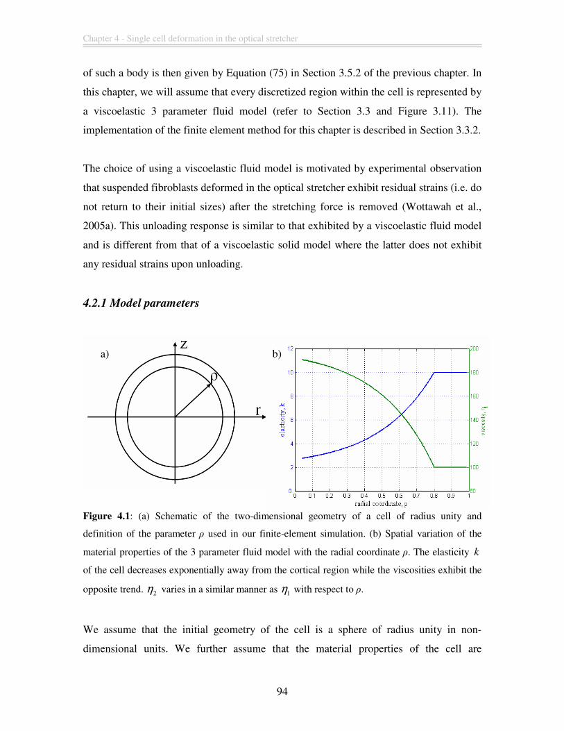
Chapter 4 - Single cell deformation in the optical stretcher
94
of such a body is then given by Equation (75) in Section 3.5.2 of the previous chapter. In
this chapter, we will assume that every discretized region within the cell is represented by
a viscoelastic 3 parameter fluid model (refer to Section 3.3 and Figure 3.11). The
implementation of the finite element method for this chapter is described in Section 3.3.2.
The choice of using a viscoelastic fluid model is motivated by experimental observation
that suspended fibroblasts deformed in the optical stretcher exhibit residual strains (i.e. do
not return to their initial sizes) after the stretching force is removed (Wottawah et al.,
2005a). This unloading response is similar to that exhibited by a viscoelastic fluid model
and is different from that of a viscoelastic solid model where the latter does not exhibit
any residual strains upon unloading.
4.2.1 Model parameters
Figure 4.1: (a) Schematic of the two-dimensional geometry of a cell of radius unity and
definition of the parameter ρ used in our finite-element simulation. (b) Spatial variation of the
material properties of the 3 parameter fluid model with the radial coordinate ρ. The elasticity k
of the cell decreases exponentially away from the cortical region while the viscosities exhibit the
opposite trend. 2η varies in a similar manner as 1η with respect to ρ.
We assume that the initial geometry of the cell is a sphere of radius unity in non-
dimensional units. We further assume that the material properties of the cell are
a) b)
Chapter 4 - Single cell deformation in the optical stretcher
95
azimuthally isotropic. Then, we can introduce the radial polar coordinate ρ of a material
point from the origin of the cell (refer to Figure 4.1a) so that the material property of each
discretized region is a function of ρ (refer to Figure 4.1b).
For normal cells, we represent the actin cortex as the region 0.8 ≤ ρ ≤ 1, i.e. with a
cortical thickness of 20% and the cytoplasm as the region 0 ≤ ρ < 0.8. This value of the
thickness of the actin cortical region in our model is similar to that used in
Ananthakrishnan et al. (2006). The actin cortical region is modelled as a predominately
elastic region with short retardation time and low viscosity (refer to Figure 4.1b). For
suspended cells, it can be shown that actin filaments are highly localized in the cortical
region (refer to Figure 4.2). We assume that the concentration of actin filaments is the
main contributor to the elasticity of our viscoelastic material model and as we move away
from the cortical region into the cytoplasm, the concentration of actin filaments decreases
significantly in a non-linear fashion. Thus, we assume that the elasticity k decreases
exponentially as ρ approaches zero. The opposite trend, an exponential increase, is
assumed for both viscosities 1η and 2η as we move away from the cortical region. This
increase in the retardation time and viscosity is to approximate the fluid-like flow
response of the cytoplasm. The spatial variation of k , 1η and 2η are described by the
equations:
( ) /( ) c c
cyto cort cytok k k k eα ρ ρ ρ− −= + − for ,
cρ ρ< (80)
cortk k= for ,
cρ ρ≥ (81)
( ) /, , ,( )(1 )c c
i i cort i cyto i cort eα ρ ρ ρη η η η − −= + − − for ,
cρ ρ< 1,2i = (82)
,i i cortη η= for ,
cρ ρ≥ 1,2i = (83)
where cort
k and ,i cortη denote the elasticity and viscosity of the cell in the cortical region,
cytok and ,i cyto
η denote the asymptotic basal elasticity and asymptotic plateau viscosity of
the cell in the cytoplasm, α is a parameter that controls the rate of exponential increase /
decrease and c
ρ is the radial polar coordinate of the interface between the cortical region
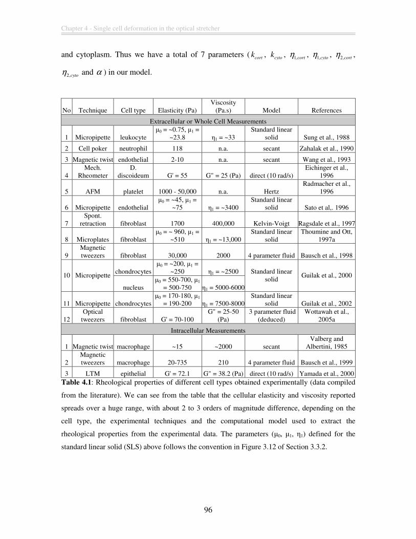
Chapter 4 - Single cell deformation in the optical stretcher
96
and cytoplasm. Thus we have a total of 7 parameters (cort
k , cyto
k , 1,cortη , 1,cyto
η , 2,cortη ,
2,cytoη and α ) in our model.
No Technique Cell type Elasticity (Pa) Viscosity
(Pa.s) Model References
Extracellular or Whole Cell Measurements
1 Micropipette leukocyte µ0 = ~0.75, µ1 =
~23.8 η1 = ~33 Standard linear
solid Sung et al., 1988
2 Cell poker neutrophil 118 n.a. secant Zahalak et al., 1990
3 Magnetic twist endothelial 2-10 n.a. secant Wang et al., 1993
4 Mech.
Rheometer D.
discoideum G' = 55 G" = 25 (Pa) direct (10 rad/s) Eichinger et al.,
1996
5 AFM platelet 1000 - 50,000 n.a. Hertz Radmacher et al.,
1996
6 Micropipette endothelial µ0 = ~45, µ1 =
~75 η1 = ~3400 Standard linear
solid Sato et al,. 1996
7 Spont.
retraction fibroblast 1700 400,000 Kelvin-Voigt Ragsdale et al., 1997
8 Microplates fibroblast µ0 = ~ 960, µ1 =
~510 η1 = ~13,000 Standard linear
solid Thoumine and Ott,
1997a
9 Magnetic tweezers fibroblast 30,000 2000 4 parameter fluid Bausch et al., 1998
chondrocytes µ0 = ~200, µ1 =
~250 η1 = ~2500 10 Micropipette
nucleus µ0 = 550-700, µ1
= 500-750 η1 = 5000-6000
Standard linear solid
Guilak et al., 2000
11 Micropipette chondrocytes µ0 = 170-180, µ1
= 190-200 η1 = 7500-8000 Standard linear
solid Guilak et al., 2002
12 Optical
tweezers fibroblast G' = 70-100 G" = 25-50
(Pa) 3 parameter fluid
(deduced) Wottawah et al.,
2005a
Intracellular Measurements
1 Magnetic twist macrophage ~15 ~2000 secant Valberg and
Albertini, 1985
2 Magnetic tweezers macrophage 20-735 210 4 parameter fluid Bausch et al., 1999
3 LTM epithelial G' = 72.1 G" = 38.2 (Pa) direct (10 rad/s) Yamada et al., 2000 Table 4.1: Rheological properties of different cell types obtained experimentally (data compiled
from the literature). We can see from the table that the cellular elasticity and viscosity reported
spreads over a huge range, with about 2 to 3 orders of magnitude difference, depending on the
cell type, the experimental techniques and the computational model used to extract the
rheological properties from the experimental data. The parameters (µ0, µ1, η1) defined for the
standard linear solid (SLS) above follows the convention in Figure 3.12 of Section 3.3.2.
Chapter 4 - Single cell deformation in the optical stretcher
97
From Table 4.1, we can see that the values of the cellular elasticity and viscosity reported
in the literature by various researchers vary over a huge range. This disparity in the
rheological properties obtained experimentally could be due to different experimental
techniques used by the different groups of researchers. For the same experimental
protocol, different cell types can also give very different values of cellular elasticity and
viscosity. The underlying computational model used to extract the elasticity and viscosity
from the experimental data also contributes to the spread of the reported values. In
choosing the parameters for our finite element model, we noted that there are enormous
degrees of freedom available for the parameters (cort
k , cyto
k , 1,cortη , 1,cyto
η , 2,cortη , 2,cyto
η )
which characterize the cellular elasticity and viscosity in our finite element model. To
reduce the size of our parameter space, we used the cellular elasticity values reported in
Table 4.1 to narrow the range of values that (cort
k , cyto
k ) are allowed to take. For example,
we note that most of the elasticity values reported using the standard linear solid (SLS)
model in Table 4.1 falls with the range from 0.75 Pa to 250 Pa (Sung et al., 1988; Sato et
al,. 1996; Guilak et al., 2000, 2002) which is roughly consistent with the estimate of the
elastic modulus (G' = 70-100 Pa) obtained by Wottawah et al. (2005a). Using this
observation, we assumed that the parameters (cort
k , cyto
k ) in our model are constrained
within this range of approximately 1 Pa to 250 Pa. In a similar manner, we can constrain
the range of the parameters ( 1,cortη , 1,cyto
η ) in our model using the values of the cellular
viscosity reported in Table 4.1. We noted that the range of cellular viscosity reported in
Table 4.1 is approximately from 30 Pa.s to 8000 Pa.s. The parameters ( 2,cortη , 2,cyto
η ) are
used to control the magnitude of the retardation time in the Kelvin-Voigt element of the
three-parameter fluid model (refer to Section 3.3.2). This retardation time corresponds to
the time-scale whereby the stress within the body is transferred and borne by the elastic
component of the Kelvin-Voigt element and do not correspond to the physical viscosity
of the cell. We assume that such transfer of stress occurs within a time-scale ranging from
fractions of seconds to seconds, and therefore constrain the parameters ( 2,cortη , 2,cyto
η ) to
approximately the same range as the parameters (cort
k , cyto
k ).
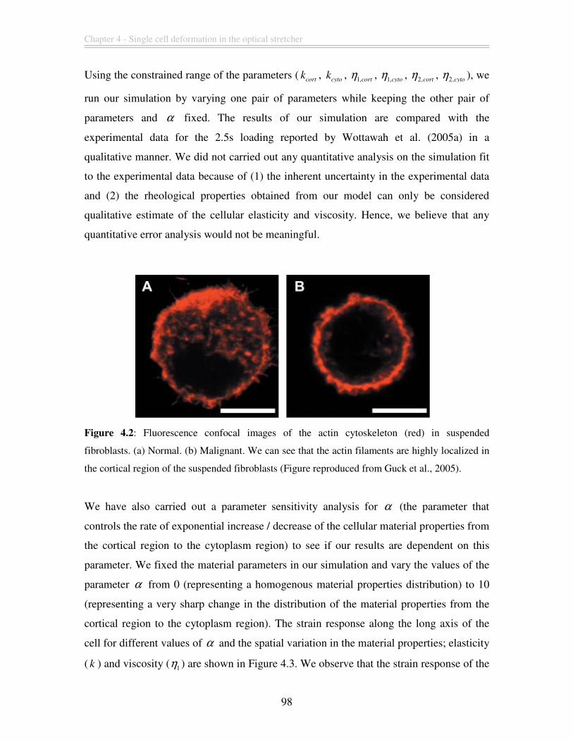
Chapter 4 - Single cell deformation in the optical stretcher
98
Using the constrained range of the parameters (cort
k , cyto
k , 1,cortη , 1,cyto
η , 2,cortη , 2,cyto
η ), we
run our simulation by varying one pair of parameters while keeping the other pair of
parameters and α fixed. The results of our simulation are compared with the
experimental data for the 2.5s loading reported by Wottawah et al. (2005a) in a
qualitative manner. We did not carried out any quantitative analysis on the simulation fit
to the experimental data because of (1) the inherent uncertainty in the experimental data
and (2) the rheological properties obtained from our model can only be considered
qualitative estimate of the cellular elasticity and viscosity. Hence, we believe that any
quantitative error analysis would not be meaningful.
Figure 4.2: Fluorescence confocal images of the actin cytoskeleton (red) in suspended
fibroblasts. (a) Normal. (b) Malignant. We can see that the actin filaments are highly localized in
the cortical region of the suspended fibroblasts (Figure reproduced from Guck et al., 2005).
We have also carried out a parameter sensitivity analysis for α (the parameter that
controls the rate of exponential increase / decrease of the cellular material properties from
the cortical region to the cytoplasm region) to see if our results are dependent on this
parameter. We fixed the material parameters in our simulation and vary the values of the
parameter α from 0 (representing a homogenous material properties distribution) to 10
(representing a very sharp change in the distribution of the material properties from the
cortical region to the cytoplasm region). The strain response along the long axis of the
cell for different values of α and the spatial variation in the material properties; elasticity
( k ) and viscosity ( 1η ) are shown in Figure 4.3. We observe that the strain response of the
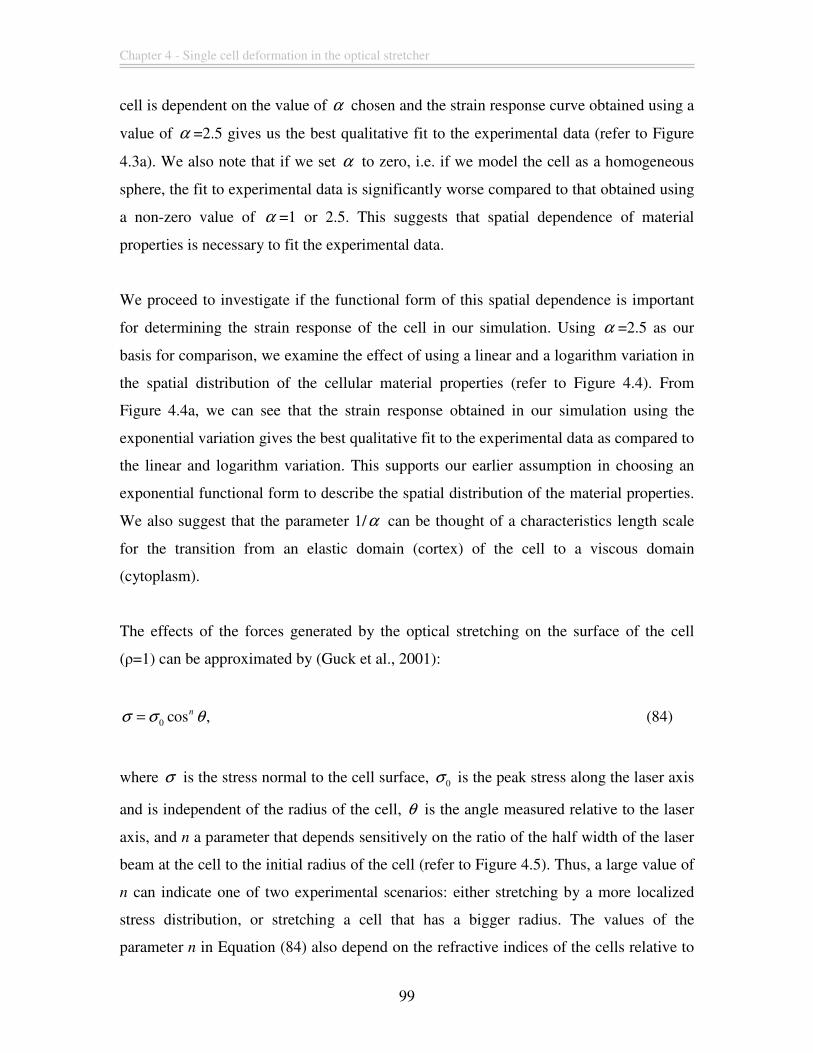
Chapter 4 - Single cell deformation in the optical stretcher
99
cell is dependent on the value of α chosen and the strain response curve obtained using a
value of α =2.5 gives us the best qualitative fit to the experimental data (refer to Figure
4.3a). We also note that if we set α to zero, i.e. if we model the cell as a homogeneous
sphere, the fit to experimental data is significantly worse compared to that obtained using
a non-zero value of α =1 or 2.5. This suggests that spatial dependence of material
properties is necessary to fit the experimental data.
We proceed to investigate if the functional form of this spatial dependence is important
for determining the strain response of the cell in our simulation. Using α =2.5 as our
basis for comparison, we examine the effect of using a linear and a logarithm variation in
the spatial distribution of the cellular material properties (refer to Figure 4.4). From
Figure 4.4a, we can see that the strain response obtained in our simulation using the
exponential variation gives the best qualitative fit to the experimental data as compared to
the linear and logarithm variation. This supports our earlier assumption in choosing an
exponential functional form to describe the spatial distribution of the material properties.
We also suggest that the parameter 1/α can be thought of a characteristics length scale
for the transition from an elastic domain (cortex) of the cell to a viscous domain
(cytoplasm).
The effects of the forces generated by the optical stretching on the surface of the cell
(ρ=1) can be approximated by (Guck et al., 2001):
0 cos ,nσ σ θ= (84)
where σ is the stress normal to the cell surface, 0σ is the peak stress along the laser axis
and is independent of the radius of the cell, θ is the angle measured relative to the laser
axis, and n a parameter that depends sensitively on the ratio of the half width of the laser
beam at the cell to the initial radius of the cell (refer to Figure 4.5). Thus, a large value of
n can indicate one of two experimental scenarios: either stretching by a more localized
stress distribution, or stretching a cell that has a bigger radius. The values of the
parameter n in Equation (84) also depend on the refractive indices of the cells relative to

Chapter 4 - Single cell deformation in the optical stretcher
100
the medium. It has been shown that the reflective indices for the malignant and normal
fibroblasts used in the optical stretcher experiments are indistinguishable (Guck et al,
2005), thus we will only consider the parameter n to be dependent on the experimental
setup. These forces are generated as a result of the differences in the dielectric constant of
the cell and the medium, and can stably trap the cell in the middle of the optical stretcher.
There is thus no need to consider effects such as cell-substrate adhesion or shape changes
owing to the cell resting on the substrate.
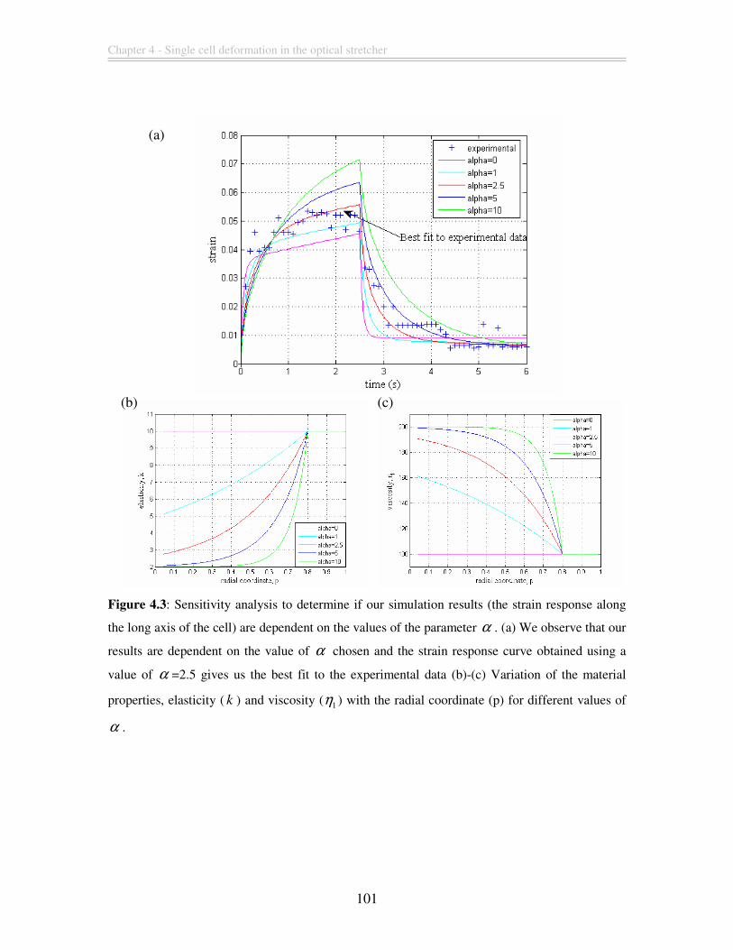
Chapter 4 - Single cell deformation in the optical stretcher
101
Figure 4.3: Sensitivity analysis to determine if our simulation results (the strain response along
the long axis of the cell) are dependent on the values of the parameter α . (a) We observe that our
results are dependent on the value of α chosen and the strain response curve obtained using a
value of α =2.5 gives us the best fit to the experimental data (b)-(c) Variation of the material
properties, elasticity ( k ) and viscosity ( 1η ) with the radial coordinate (p) for different values of
α .
(a)
(b) (c)
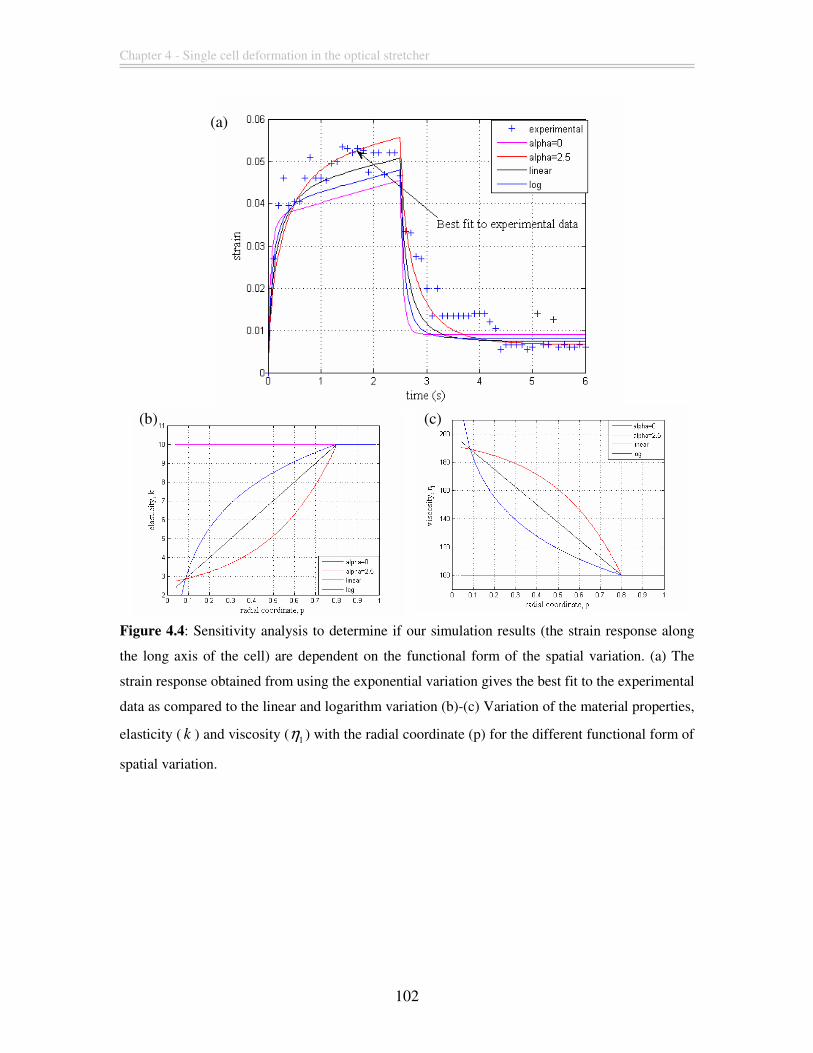
Chapter 4 - Single cell deformation in the optical stretcher
102
Figure 4.4: Sensitivity analysis to determine if our simulation results (the strain response along
the long axis of the cell) are dependent on the functional form of the spatial variation. (a) The
strain response obtained from using the exponential variation gives the best fit to the experimental
data as compared to the linear and logarithm variation (b)-(c) Variation of the material properties,
elasticity ( k ) and viscosity ( 1η ) with the radial coordinate (p) for the different functional form of
spatial variation.
(c)
(a)
(b)
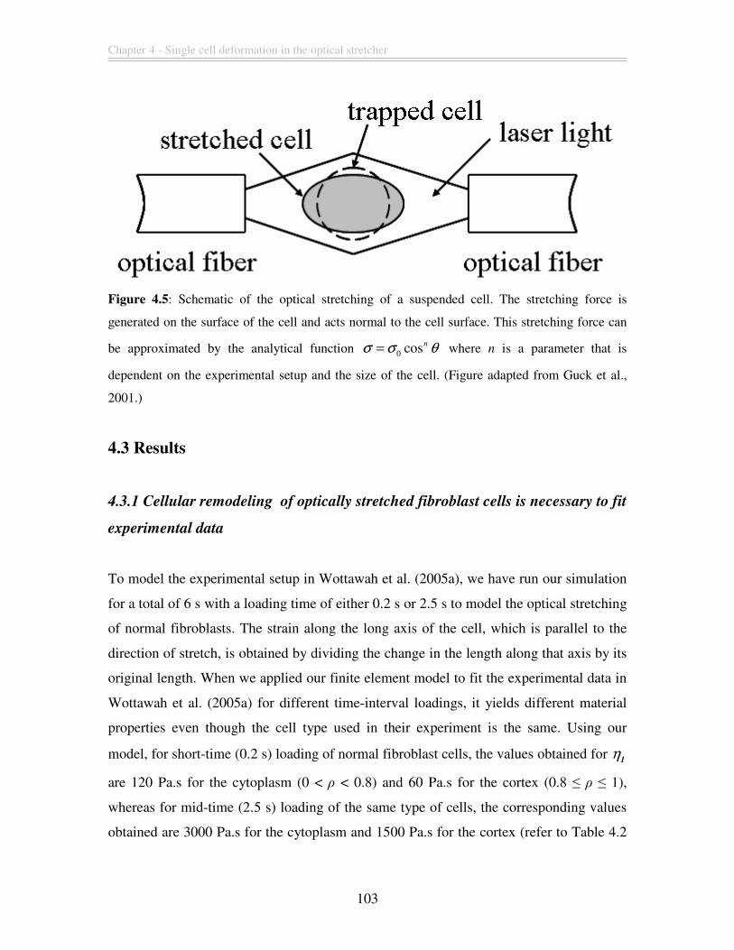
Chapter 4 - Single cell deformation in the optical stretcher
103
Figure 4.5: Schematic of the optical stretching of a suspended cell. The stretching force is
generated on the surface of the cell and acts normal to the cell surface. This stretching force can
be approximated by the analytical function 0 cosnσ σ θ= where n is a parameter that is
dependent on the experimental setup and the size of the cell. (Figure adapted from Guck et al.,
2001.)
4.3 Results
4.3.1 Cellular remodeling of optically stretched fibroblast cells is necessary to fit
experimental data
To model the experimental setup in Wottawah et al. (2005a), we have run our simulation
for a total of 6 s with a loading time of either 0.2 s or 2.5 s to model the optical stretching
of normal fibroblasts. The strain along the long axis of the cell, which is parallel to the
direction of stretch, is obtained by dividing the change in the length along that axis by its
original length. When we applied our finite element model to fit the experimental data in
Wottawah et al. (2005a) for different time-interval loadings, it yields different material
properties even though the cell type used in their experiment is the same. Using our
model, for short-time (0.2 s) loading of normal fibroblast cells, the values obtained for 1
η
are 120 Pa.s for the cytoplasm (0 < ρ < 0.8) and 60 Pa.s for the cortex (0.8 ≤ ρ ≤ 1),
whereas for mid-time (2.5 s) loading of the same type of cells, the corresponding values
obtained are 3000 Pa.s for the cytoplasm and 1500 Pa.s for the cortex (refer to Table 4.2
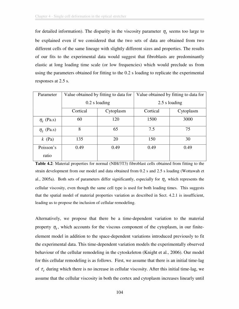
Chapter 4 - Single cell deformation in the optical stretcher
104
for detailed information). The disparity in the viscosity parameter 1
η seems too large to
be explained even if we considered that the two sets of data are obtained from two
different cells of the same lineage with slightly different sizes and properties. The results
of our fits to the experimental data would suggest that fibroblasts are predominantly
elastic at long loading time scale (or low frequencies) which would preclude us from
using the parameters obtained for fitting to the 0.2 s loading to replicate the experimental
responses at 2.5 s.
Value obtained by fitting to data for
0.2 s loading
Value obtained by fitting to data for
2.5 s loading
Parameter
Cortical Cytoplasm Cortical Cytoplasm
1η (Pa.s) 60 120 1500 3000
2η (Pa.s) 8 65 7.5 75
k (Pa) 135 20 150 30
Poisson’s
ratio
0.49 0.49 0.49 0.49
Table 4.2: Material properties for normal (NIH/3T3) fibroblast cells obtained from fitting to the
strain development from our model and data obtained from 0.2 s and 2.5 s loading (Wottawah et
al., 2005a). Both sets of parameters differ significantly, especially for 1
η which represents the
cellular viscosity, even though the same cell type is used for both loading times. This suggests
that the spatial model of material properties variation as described in Sect. 4.2.1 is insufficient,
leading us to propose the inclusion of cellular remodeling.
Alternatively, we propose that there be a time-dependent variation to the material
property 1
η , which accounts for the viscous component of the cytoplasm, in our finite-
element model in addition to the space-dependent variations introduced previously to fit
the experimental data. This time-dependent variation models the experimentally observed
behaviour of the cellular remodeling in the cytoskeleton (Knight et al., 2006). Our model
for this cellular remodeling is as follows. First, we assume that there is an initial time-lag
of τ1 during which there is no increase in cellular viscosity. After this initial time-lag, we
assume that the cellular viscosity in both the cortex and cytoplasm increases linearly until
Chapter 4 - Single cell deformation in the optical stretcher
105
it reaches a steady-state value and does not increase further. We further assume that this
steady-state is reached after a time-duration denoted by τ2. The temporal variation of the
viscosity 1
η during this remodeling phase is described by the equation:
11 k 1 k init 1 k final 1 k init
2
t τη η η η
τ
−= + −
, , _ , _ , _( ) for
1 1 2tτ τ τ< < + , (85)
where the subscript k denotes either cort or cyto, 1 cort init, _
η and 1 cyto init, _
η denotes the
cortical and cytoplasmic plateau viscosity of the cell prior to the cellular remodeling (for
1t τ≤ ),
1 cort final, _η and
1 cyto final, _η denotes the cortical and cytoplasmic plateau viscosity of
the cell after the cellular remodeling (for 1 2
t τ τ> + ). The spatial variation of the
viscosity 1
η during the cellular remodeling phase is still described by Equations (82) and
(83). The parameters τ1 and τ
2 will give us a quantitative estimate of the rate at which
the cytoskeleton remodeling takes place.
From our simulations, we obtained both τ1 and τ
2 to be 0.2 s and the magnitude of the
viscosity 1
η was found to vary from 150 Pa.s (1 cort init, _
η ) prior to the cellular remodeling
to 3000 Pa.s (1 cort final, _
η ) after the cellular remodeling in the cortical region, and similarly
from 300 Pa.s (1 cyto init, _
η ) to 6000 Pa.s (1 cyto final, _
η ) in the cytoplasm (refer to Table 4.3 for
detailed information). We plotted the results of fitting our model incorporating cellular
remodeling to two sets of experimental data for the strain development, namely data for
0.2 s loading and data for 2.5 s loading in Figure 4.6. We reiterate that the fits to both sets
of data are performed using the same set of spatiotemporally-varying parameters. The
only free parameter in our model is a scaling factor which is used to rescale the
experimental data because the peak stress for the 0.2 s and 2.5 s experimental loadings
are different.
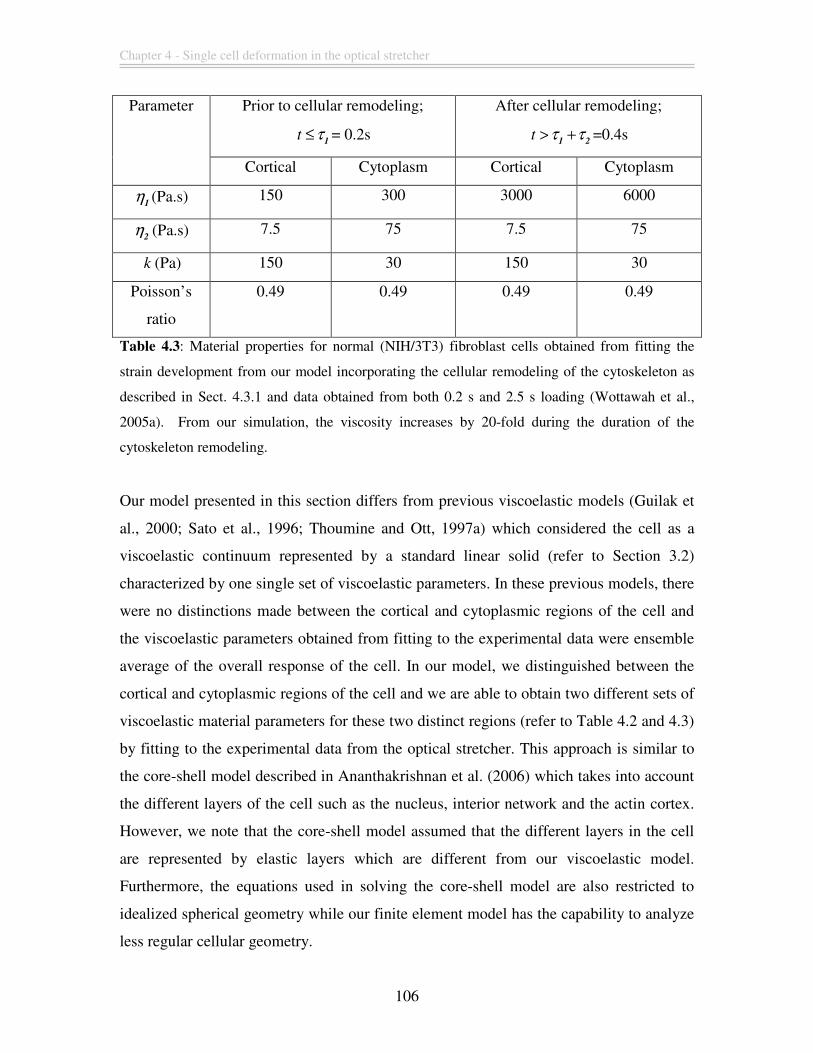
Chapter 4 - Single cell deformation in the optical stretcher
106
Prior to cellular remodeling;
t τ≤1= 0.2s
After cellular remodeling;
t τ τ> +1 2
=0.4s
Parameter
Cortical Cytoplasm Cortical Cytoplasm
1η (Pa.s) 150 300 3000 6000
2η (Pa.s) 7.5 75 7.5 75
k (Pa) 150 30 150 30
Poisson’s
ratio
0.49 0.49 0.49 0.49
Table 4.3: Material properties for normal (NIH/3T3) fibroblast cells obtained from fitting the
strain development from our model incorporating the cellular remodeling of the cytoskeleton as
described in Sect. 4.3.1 and data obtained from both 0.2 s and 2.5 s loading (Wottawah et al.,
2005a). From our simulation, the viscosity increases by 20-fold during the duration of the
cytoskeleton remodeling.
Our model presented in this section differs from previous viscoelastic models (Guilak et
al., 2000; Sato et al., 1996; Thoumine and Ott, 1997a) which considered the cell as a
viscoelastic continuum represented by a standard linear solid (refer to Section 3.2)
characterized by one single set of viscoelastic parameters. In these previous models, there
were no distinctions made between the cortical and cytoplasmic regions of the cell and
the viscoelastic parameters obtained from fitting to the experimental data were ensemble
average of the overall response of the cell. In our model, we distinguished between the
cortical and cytoplasmic regions of the cell and we are able to obtain two different sets of
viscoelastic material parameters for these two distinct regions (refer to Table 4.2 and 4.3)
by fitting to the experimental data from the optical stretcher. This approach is similar to
the core-shell model described in Ananthakrishnan et al. (2006) which takes into account
the different layers of the cell such as the nucleus, interior network and the actin cortex.
However, we note that the core-shell model assumed that the different layers in the cell
are represented by elastic layers which are different from our viscoelastic model.
Furthermore, the equations used in solving the core-shell model are also restricted to
idealized spherical geometry while our finite element model has the capability to analyze
less regular cellular geometry.
Chapter 4 - Single cell deformation in the optical stretcher
107
The value of the cortical elasticity obtained from our cellular remodelling model is
comparable to the elasticity for the actin cortical shell from the core-shell model. This is
not surprising since both models consider the cell to be comprised of distinct regions.
However, we note that comparison of the viscosity values between the two models is not
possible since they assumed elastic properties. The viscosity values of the cortical and
cytoplasmic regions that we obtained from our simulation fall within the range of
experimental values that have been reported for fibroblast cells (Bausch et al., 1998;
Karcher et al., 2003; Thoumine and Ott, 1997a). For example, microplate manipulation of
adhered fibroblasts reported the overall cellular viscosity to be approximately 10000 Pa.s
based on a three-parameter viscoelastic solid model (Thoumine and Ott, 1997a) while
measurements based on magnetic tweezers reported a value of approximately 2000 Pa.s
(Bausch et al., 1998). Furthermore, experiments performed on quiescent and migrating
fibroblasts reported an approximate 5-fold increase in the intracellular shear viscosity
(Kole et al., 2005), and that migrating fibroblasts exhibit a compliance of about an order
of magnitude difference from its leading edge (lower compliance) to its perinuclear
regions (higher compliance) (Kole et al., 2005). We note that the rate of the cellular
remodeling and the magnitude of the increase in the cellular viscosity as obtained from
our model (approximately 20-fold increase in 0.2s) has not been observed
experimentally. Shear flow studies done on adherent fibroblasts have shown that fluid
flow induces an approximately 25-fold increase in cytoplasmic viscosity but only after 40
minutes (Lee et al., 2006). As such, this discrepancy between the time scales for the
cellular response as obtained from our model and the experimental observations in Lee et
al. (2006) could be attributed to different mechanisms being activated by the cells in the
two experimental setup. The accuracy of our parameters from the cellular remodeling
model is also strongly dependent on the accuracy of the experimental data from the
optical stretcher experiment. Given the inherent uncertainties in the experimental data,
we acknowledge the uncertainties in our predicted time scale of the cellular remodeling
and note that such responses could take place over a time scale ranging from fractions of
seconds to minutes.
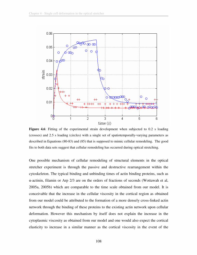
Chapter 4 - Single cell deformation in the optical stretcher
108
Figure 4.6: Fitting of the experimental strain development when subjected to 0.2 s loading
(crosses) and 2.5 s loading (circles) with a single set of spatiotemporally-varying parameters as
described in Equations (80-83) and (85) that is supposed to mimic cellular remodeling. The good
fits to both data sets suggest that cellular remodeling has occurred during optical stretching.
One possible mechanism of cellular remodeling of structural elements in the optical
stretcher experiment is through the passive and destructive rearrangement within the
cytoskeleton. The typical binding and unbinding times of actin binding proteins, such as
α-actinin, filamin or Arp 2/3 are on the orders of fractions of seconds (Wottawah et al,
2005a, 2005b) which are comparable to the time scale obtained from our model. It is
conceivable that the increase in the cellular viscosity in the cortical region as obtained
from our model could be attributed to the formation of a more densely cross-linked actin
network through the binding of these proteins to the existing actin network upon cellular
deformation. However this mechanism by itself does not explain the increase in the
cytoplasmic viscosity as obtained from our model and one would also expect the cortical
elasticity to increase in a similar manner as the cortical viscosity in the event of the
Chapter 4 - Single cell deformation in the optical stretcher
109
formation of a more densely cross-linked actin network. The results from our simulation
suggest otherwise as the cortical elasticity does not vary in a time-dependent manner,
unlike the cortical viscosity. It could be possible, though unlikely, that another set of
time-dependent cortical elasticity and viscosity could be used to fit both sets of
experiment data from the optical stretcher experiment while keeping the cytoplasm
elasticity and viscosity time-independent. Such a combination of mechanical properties
will then offer stronger support to the mechanism of passive and destructive
rearrangement within the cytoskeleton through the binding and unbinding of actin
binding proteins.
Another possible mechanism to explain the increased in cellular viscosity was published
just prior to the submission of this thesis (Ebert et al, 2007). It involves the heating effect
generated by the optical stretcher. It was reported that the temperature in the trap
increases by about 30ºC within 0.2 s in the optical stretcher experimental setup. Such a
temperature increase could possibly trigger changes in the mechanical properties of the
fibroblasts during the course of the experiments. This “thermal shock” acting on the cell
could possibly explain the mechanism for the increase in the cellular viscosity obtained
from our model and the time scale at which this cellular remodeling occurs. It could also
help to explain the discrepancies in the time scale between our simulation results and
existing experimental observations as discussed previously. The results from our model
that cellular remodeling occurs in the optical stretcher in terms of a change in the cellular
viscosity could be viewed as a “discovery” of the effect of the temperature increase on
the mechanical response of the cell in the optical stretcher.
The cell nucleus was omitted in our model formulation in this chapter but we noted that
the inclusion of a fairly sizeable nucleus, which can be considered largely elastic, at the
centre of the cell can be easily incorporated into our model formulation without any
significant difficulties. Given that the strains experienced by the cells in the optical
stretcher is less than 6% for loading duration up to 2.5 s (refer to Figure 4.6), the potential
impact of including the cell nucleus will likely be relatively small and should not affect
the qualitative trend of the cellular remodelling as presented above. For longer loading
Chapter 4 - Single cell deformation in the optical stretcher
110
duration beyond 2.5 s and larger cellular strains, the contribution of the nucleus to the
cellular deformability will become increasingly important. In such situation, the presence
of a sizeable and largely elastic nucleus in the computational model will have to be taken
into account in order to obtain a realistic description of the cellular deformation.
4.3.2. Maximal strain developed depends on size of suspended fibroblast cells
being stretched
From experiments (Guck et al., 2005; Ananthakrishnan et al., 2006), we know that the
optical deformability of malignantly transformed SV-T2 fibroblast cells is significantly
higher than that of normal NIH/3T3 fibroblast cells. The optical deformability is the
strain normalized by the stretching force that the cell experienced (refer to Guck et al.,
2005 for definition). From the data in Guck et al. (2005), we estimate that the mean
optical deformability of malignant fibroblasts is about 40% higher compared to that of
normal fibroblasts. It has been suggested (Guck et al., 2005) that the thickness of the
actin cortical region plays an important role in determining this difference. In this section,
we show that cell size (through its effect on the surface stretching profile) is a more
important factor in determining the maximal strain developed (and hence the optical
deformability) than the thickness of the actin cortical region.
In Table 4.4, we list some of the differences between normal and malignant fibroblast
cells. Normal fibroblast cells generally have a larger radius and also a thicker actin
cortical region as compared to malignant fibroblast cells. The larger radius of the normal
cells means that the value of the parameter n in Equation (84), that characterizes the
spread of the stress distribution, is higher. Thus, they are being subjected to a more
localized stress distribution, under the same optical setup, as compared to the malignant
cells (Ananthakrishnan et al., 2006). The range of the parameter n for normal fibroblasts
in the optical stretcher lies from 14 to 24, while as the range for malignant fibroblasts lies
from 4 to 14. We want to show quantitatively how these two factors, namely the cell size
(and equivalently, the spread of the stress distribution) and the relative thickness of the
cortical region, affect the strain development.
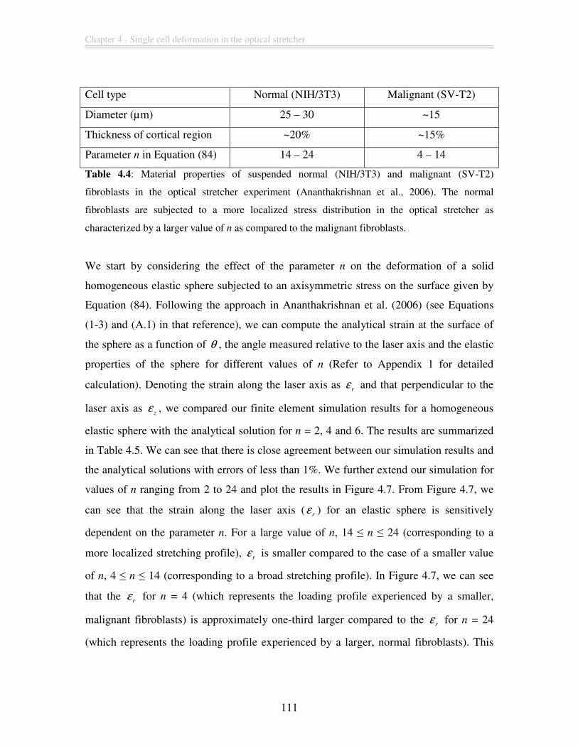
Chapter 4 - Single cell deformation in the optical stretcher
111
Cell type Normal (NIH/3T3) Malignant (SV-T2)
Diameter (µm) 25 – 30 ~15
Thickness of cortical region ~20% ~15%
Parameter n in Equation (84) 14 – 24 4 – 14
Table 4.4: Material properties of suspended normal (NIH/3T3) and malignant (SV-T2)
fibroblasts in the optical stretcher experiment (Ananthakrishnan et al., 2006). The normal
fibroblasts are subjected to a more localized stress distribution in the optical stretcher as
characterized by a larger value of n as compared to the malignant fibroblasts.
We start by considering the effect of the parameter n on the deformation of a solid
homogeneous elastic sphere subjected to an axisymmetric stress on the surface given by
Equation (84). Following the approach in Ananthakrishnan et al. (2006) (see Equations
(1-3) and (A.1) in that reference), we can compute the analytical strain at the surface of
the sphere as a function of θ , the angle measured relative to the laser axis and the elastic
properties of the sphere for different values of n (Refer to Appendix 1 for detailed
calculation). Denoting the strain along the laser axis as r
ε and that perpendicular to the
laser axis as z
ε , we compared our finite element simulation results for a homogeneous
elastic sphere with the analytical solution for n = 2, 4 and 6. The results are summarized
in Table 4.5. We can see that there is close agreement between our simulation results and
the analytical solutions with errors of less than 1%. We further extend our simulation for
values of n ranging from 2 to 24 and plot the results in Figure 4.7. From Figure 4.7, we
can see that the strain along the laser axis (r
ε ) for an elastic sphere is sensitively
dependent on the parameter n. For a large value of n, 14 ≤ n ≤ 24 (corresponding to a
more localized stretching profile), r
ε is smaller compared to the case of a smaller value
of n, 4 ≤ n ≤ 14 (corresponding to a broad stretching profile). In Figure 4.7, we can see
that the r
ε for n = 4 (which represents the loading profile experienced by a smaller,
malignant fibroblasts) is approximately one-third larger compared to the r
ε for n = 24
(which represents the loading profile experienced by a larger, normal fibroblasts). This
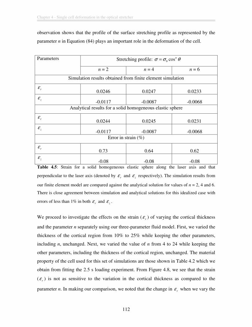
Chapter 4 - Single cell deformation in the optical stretcher
112
observation shows that the profile of the surface stretching profile as represented by the
parameter n in Equation (84) plays an important role in the deformation of the cell.
Stretching profile: 0 cosnσ σ θ= Parameters
n = 2 n = 4 n = 6
Simulation results obtained from finite element simulation
rε
0.0246 0.0247 0.0233
zε
-0.0117 -0.0087 -0.0068 Analytical results for a solid homogeneous elastic sphere
rε
0.0244 0.0245 0.0231
zε
-0.0117 -0.0087 -0.0068 Error in strain (%)
rε
0.73 0.64 0.62
zε
-0.08 -0.08 -0.08 Table 4.5: Strain for a solid homogeneous elastic sphere along the laser axis and that
perpendicular to the laser axis (denoted by r
ε and z
ε respectively). The simulation results from
our finite element model are compared against the analytical solution for values of n = 2, 4 and 6.
There is close agreement between simulation and analytical solutions for this idealized case with
errors of less than 1% in both r
ε and z
ε .
We proceed to investigate the effects on the strain (
rε ) of varying the cortical thickness
and the parameter n separately using our three-parameter fluid model. First, we varied the
thickness of the cortical region from 10% to 25% while keeping the other parameters,
including n, unchanged. Next, we varied the value of n from 4 to 24 while keeping the
other parameters, including the thickness of the cortical region, unchanged. The material
property of the cell used for this set of simulations are those shown in Table 4.2 which we
obtain from fitting the 2.5 s loading experiment. From Figure 4.8, we see that the strain
(r
ε ) is not as sensitive to the variation in the cortical thickness as compared to the
parameter n. In making our comparison, we noted that the change in r
ε when we vary the
Chapter 4 - Single cell deformation in the optical stretcher
113
cortical thickness is fairly independent of the values of the parameter n. Hence, we
decided to choose an arbitrary value of n (we used n = 18 in Figure 4.8) to illustrate the
typical effect of varying the cortical thickness on r
ε . To illustrate the effect of the
parameter n on r
ε , we have chosen n = 8 and n = 20, which are the mid-range values for
characterizing the load profile experienced by the malignant and normal fibroblasts
respectively. We also observe that the strains r
ε are smaller for a larger value of n when
compared to those of a smaller n which is similar to the trend exhibited by the
homogeneous elastic sphere. Thus, our simulation supports the experimental evidence
that the smaller malignant cells deform more compared to their normal counterparts.
However, we propose that the size of the cell explains this difference in the radial
deformation rather than the difference in the cortical thickness as proposed by Guck et
al., 2005.
We note that our simulation results that the smaller malignant cells deform more
compared to their normal counterparts rests on the assumption that the optical properties
are fairly homogenous in both the malignant and normal fibroblasts. It is possible that
there will be regions in the cell with different optical properties, which could lead to a
very different distribution of stress on the surface. One possible example is a smaller
malignant fibroblast with a relatively large nucleus with higher refractive index, which
could lead to a stronger focusing of the light passing through the cell and consequently a
more localized stress distribution than assumed. In this case, the explanation for the
different deformability between the normal and malignant fibroblasts suggested from our
model might not hold. Given the complexity of the actual stress distribution on the cell
surface during the experiments, we believe that our model can still contribute to the
understanding of the differences in cellular response between malignant and normal
fibroblasts in the optical stretcher despite our simple assumptions.
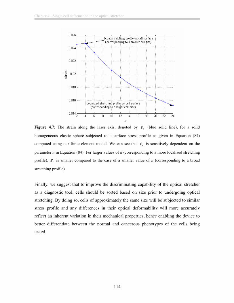
Chapter 4 - Single cell deformation in the optical stretcher
114
Figure 4.7: The strain along the laser axis, denoted by
rε (blue solid line), for a solid
homogeneous elastic sphere subjected to a surface stress profile as given in Equation (84)
computed using our finite element model. We can see that r
ε is sensitively dependent on the
parameter n in Equation (84). For larger values of n (corresponding to a more localised stretching
profile), r
ε is smaller compared to the case of a smaller value of n (corresponding to a broad
stretching profile).
Finally, we suggest that to improve the discriminating capability of the optical stretcher
as a diagnostic tool, cells should be sorted based on size prior to undergoing optical
stretching. By doing so, cells of approximately the same size will be subjected to similar
stress profile and any differences in their optical deformability will more accurately
reflect an inherent variation in their mechanical properties, hence enabling the device to
better differentiate between the normal and cancerous phenotypes of the cells being
tested.
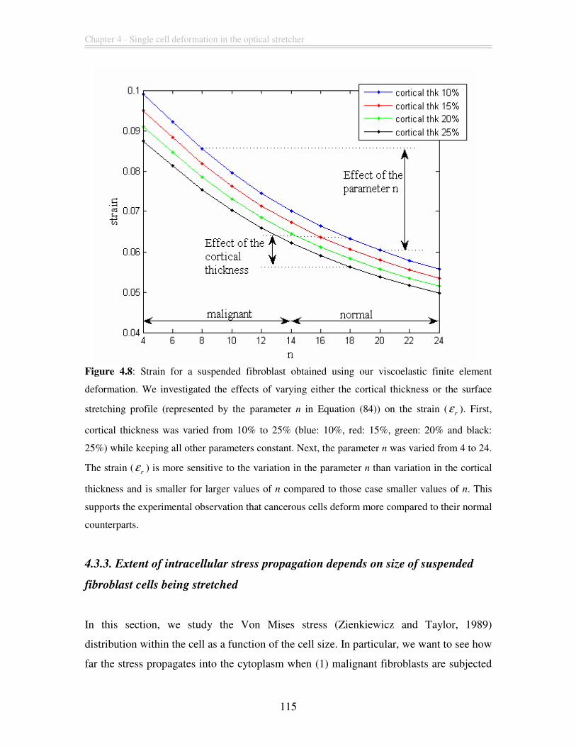
Chapter 4 - Single cell deformation in the optical stretcher
115
Figure 4.8: Strain for a suspended fibroblast obtained using our viscoelastic finite element
deformation. We investigated the effects of varying either the cortical thickness or the surface
stretching profile (represented by the parameter n in Equation (84)) on the strain (r
ε ). First,
cortical thickness was varied from 10% to 25% (blue: 10%, red: 15%, green: 20% and black:
25%) while keeping all other parameters constant. Next, the parameter n was varied from 4 to 24.
The strain (r
ε ) is more sensitive to the variation in the parameter n than variation in the cortical
thickness and is smaller for larger values of n compared to those case smaller values of n. This
supports the experimental observation that cancerous cells deform more compared to their normal
counterparts.
4.3.3. Extent of intracellular stress propagation depends on size of suspended
fibroblast cells being stretched
In this section, we study the Von Mises stress (Zienkiewicz and Taylor, 1989)
distribution within the cell as a function of the cell size. In particular, we want to see how
far the stress propagates into the cytoplasm when (1) malignant fibroblasts are subjected
Chapter 4 - Single cell deformation in the optical stretcher
116
to a broad surface stress distribution and (2) normal fibroblasts are subjected to a
localized surface stress distribution. The Von Mises stress from our simulation is
computed using the spring element in the three-parameter viscoelastic fluid model. The
details of the simulation are: the material properties of both the normal and malignant
fibroblasts are set to identical values (values used in this simulation are shown in Table
4.2 from fitting to the 2.5 s loading experiment). The thickness of the actin cortical region
is set to 20% for normal cells and 15% for malignant cells following the experimental
observation of Ananthakrishnan et al., 2006.
In Figure 4.9, we show the Von Mises stress distribution at 2.5 s for the two simulations
described above. The two surface stretching profiles are represented by (a) n = 24
(localized stress distribution) denoting normal cells and (b) n = 4 (broad stress
distribution) denoting malignant cells. For the localized stress distribution, we see that the
regions with the highest Von Mises stress concentration are offset from the centre of the
cell and occur at a region just beneath the cortical region. This observation is distinctly
different from that observed for the broad stress distribution in which the region of
highest Von Mises stress is in the perinuclear region of the cell.
This observation is insightful as it allows us to track the stress propagation from the
cortical region through to the cytoplasm as a function of the surface stretching profile.
We hypothesize that the two distinct regions of high Von Mises stress concentration for
the localized stretching profile could be a result of the short length-scale force
transmission characteristics of the cytoplasm (Guilak et al., 2000). When a mechanical
loading applied to the cell is concentrated on a localized region of its cortex or cytoplasm,
the cellular response will depend on the region being probed. Experimental techniques
that apply a localized loading include atomic force microscopy, magnetic bead twisting
and micropipette aspiration techniques as discussed in Section 2.2.1. On the other end of
the spectrum, when the entire cell is subjected to mechanical stress, such as a shear flow
or microplate manipulation (refer to Section 2.2.2), the cellular response will depend
upon the overall compliance of the entire cell. This could also be a reason that explains
the huge spread of experimental values reported for both the elasticity and viscosity

Chapter 4 - Single cell deformation in the optical stretcher
117
values. Such measurements will depend not only on the model used to extract the
relevant elastic or viscous parameters but also, to a large extent, on the region of the cell
being probed and the extent of the probing mechanisms (whether it acts over a localized
region or the entire cell).
We further hypothesize that different mechanosensitive pathways might be activated in
the optical stretching experiment as a result of the differences in the relative stress
distribution within the interior of the suspended cell. One possible mechanism is for the
cell to upregulate the concentrations of actin binding proteins in response to signalling
pathways that are mediated through the stretch activated channels (Martinac, 2004;
Sukharev and Corey, 2004). We postulate that these activated channels then transduce the
external mechanical forces into intracellular biochemical signals through the increase in
the cytosolic Ca2+ level (Munevar et al., 2004) which in turn triggers a cascade of
signalling pathways (Janmey, 1998). One such possible signalling pathway is the
Rho/Rho-kinase transduction pathway which is involved in the cytoplasmic stiffening of
adherent fibroblasts subjected to shear flow (Lee et al., 2006). We thus suggest that
fluorescent tagging be done on actin binding proteins such as filamin A to investigate
how their concentration in the cortical regions varies as the suspended fibroblasts are
subjected to different stretching profiles. Such investigations could allow us to directly
relate our simulation results of the location of high Von Mises stress to experimental
observations on the regions of high activity of actin binding proteins.
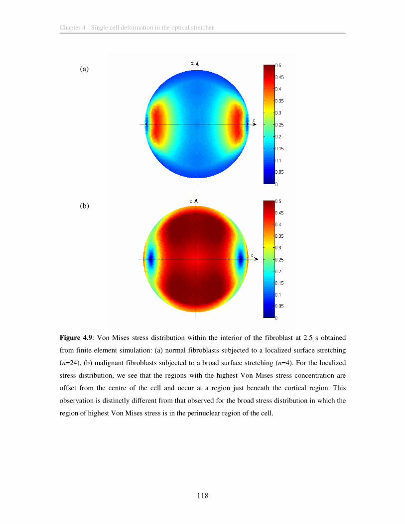
Chapter 4 - Single cell deformation in the optical stretcher
118
Figure 4.9: Von Mises stress distribution within the interior of the fibroblast at 2.5 s obtained
from finite element simulation: (a) normal fibroblasts subjected to a localized surface stretching
(n=24), (b) malignant fibroblasts subjected to a broad surface stretching (n=4). For the localized
stress distribution, we see that the regions with the highest Von Mises stress concentration are
offset from the centre of the cell and occur at a region just beneath the cortical region. This
observation is distinctly different from that observed for the broad stress distribution in which the
region of highest Von Mises stress is in the perinuclear region of the cell.
(a)
(b)
Chapter 4 - Single cell deformation in the optical stretcher
119
4.4. Conclusion
We have described a viscoelastic, axisymmetric finite-element model that takes into
account the spatiotemporal heterogeneity of cells and have shown that our model can be
used to simulate the stretching of suspended fibroblast cells in the optical stretcher. The
first result of this chapter is that cellular remodeling, in the form of an increase in the
cellular viscosity, is necessary in order to fit our simulation results to the experimentally-
observed strain development for both 0.2 s and 2.5 s loading (Wottawah et al., 2005a).
We note that the rate of this cellular remodeling and the magnitude of the increase in the
cellular viscosity have not yet been observed in experiments. The discrepancy in the time
scale of the cellular remodeling as predicted by our model and existing experimental data
could be attributed to different response mechanisms activated by the cells being probed
and suggested that cellular responses can occur over a wide range of time scale ranging
from fractions of seconds to minutes. It is also likely that the mechanism of this cellular
remodeling can be attributed to the heating effects induced by the optical stretcher where
the temperature in the trap increases approximately 30ºC within 0.2 s (Ebert et al., 2007).
The time scale of this “thermal shock” corresponds very well to the time scale of the
cellular remodeling as obtained from our model and could help explain the discrepancies
in the time scale between our simulation results and existing experimental observations.
The second result of the chapter is that the higher optical deformability observed for
malignant fibroblasts (Guck et al., 2005) can be explained by the difference in the surface
stretching profile (which is related to the cell size). We have shown that the parameter n
which describes the profile of the stretching load is a more important factor in
determining the radial deformation of the cell than the thickness of the actin cortical
region. This implies that cells with a smaller radius will experience more stretching
compared to cells with a larger radius in the optical stretcher due to the broader stress
profile experienced.
The final result suggests that the modes of stress propagation into the cytoplasm are
different for normal and malignant fibroblasts. Our simulation shows that the Von Mises
Chapter 4 - Single cell deformation in the optical stretcher
120
stress distribution within the cell is dependent on the surface stretching profiles used. For
the localized stretching profile, the regions with the highest Von Mises stress
concentration are offset from the centre of the cell and occur at a region just beneath the
cortical region. This pattern is distinctly different from that observed for the broad stress
distribution in which the region of highest Von Mises stress is in the perinuclear region of
the cell. Our simulation also suggests that different mechanosensitive pathways might be
activated in the optical stretching experiment as a result of this difference in the relative
stress distribution within the interior of the suspended cell.
Chapter 5 - Single cell deformation in the tapered micropipette
121
Chapter 5. Single cell deformation in the tapered
micropipette
This chapter will first give a brief introduction to the tapered micropipette experiment on
neutrophils and we will briefly discuss the finite element formulation in the context of
modeling this experiment. The geometry of our model and the heuristics used for
implementing non-penetration of the neutrophil against the pipette wall will also be
discussed. This will be followed by presentation and discussion of the results obtained
from our simulations
5.1 Introduction
Neutrophils are the most abundant type of white blood cells in humans and form an
integral part of the immune system. In normal microcirculation, neutrophils circulate
continually without obstructing flow, passing from the capillary network through the
arterioles to the venules. The typical diameter of a neutrophil ranges from 8-10 µm while
the diameter of a typical pulmonary capillary ranges from 2-15 µm (Doerschuk et al.,
1993). Thus, we can see that neutrophils will have to undergo varying degrees of
deformation as they encounter the narrower capillaries in the microcirculation. It has
been estimated that a typical flow pathway for a neutrophil encompasses about 50 to 100
such capillary segments (Hogg, 1987; Hogg et al., 1994). Experimental measurement has
also shown that neutrophils take on a nearly spherical shape in the arterioles (vessels with
an inner diameter up to 100 µm) (Popel and Johnson, 2005) and an elongated shape in the
narrow capillary segments, thereby confirming the view that neutrophils deform as they
enter the narrower capillary segments (Doerschuk et al., 1993; Gebb et al., 1995).
Mechanical forces have been recognized to play an important role in modulating and
regulating many different cellular processes such as proliferation, migration and
differentiation (Huang and Ingber, 1999; Wang et al., 1993; Wang and Ingber, 1994;
Ingber, 2003b; Huang et al., 2004). In the context of atherosclerosis, the importance of
Chapter 5 - Single cell deformation in the tapered micropipette
122
such mechanical regulation has primarily focused on endothelial cells and their response
to wall shear stresses (Giddens et al., 1993; Malek et al., 1999). Neutrophil and leukocyte
activities are generally assumed to be mediated by biochemical factors; mechanical
stimuli are usually ignored. However, recent studies have shown that both neutrophils
and leukocytes are sensitive to mechanical stimulation. Fluid shear stress can influence
the adhesion of leukocytes to substrates, the stiffness of their cytoskeleton and their
formation of pseudopods (Moazzam et al., 1997; Coughlin and Schmid-Schonbein,
2004). Mechanical deformation of neutrophils above a certain threshold has also been
shown to result in neutrophil activation with the formation of pseudopods (Yap and
Kamm, 2005a; Yap and Kamm, 2005b). Such activation is also accompanied by a
reduction in the elastic and loss modulus which is observed within seconds after onset of
mechanical stimulus, suggesting a sudden disruption of the neutrophil cytoskeleton when
subjected to mechanical deformation (Yap and Kamm, 2005a). These experimental
observations suggest that leukocytes and neutrophils have the capability of sensing
mechanical forces or deformation and are able to respond to such stimulus by altering
their rheological properties.
One of the most extensively used and well established experimental techniques for
measuring the rheological properties of neutrophils is the micropipette aspiration method
(Sung et al., 1982; Dong et al., 1991; Ting-Beall et al., 1993). This method involves the
application of a fixed suction pressure above a critical threshold to deform the neutrophil
into the narrow pipette. The ratio of the aspirated length to the inner radius of the pipette
is recorded as a function of time in the micropipette aspiration experiment (Hochmuth,
2000). In order to extract the rheological properties from this experimental observation,
neutrophils are usually modeled using the family of cortical shell-liquid core models
(refer to Section 2.3.2.1). The rheological properties thus deduced assume that the
neutrophils are passive during their deformation into the pipette and do not change their
properties with time. However, such an assumption seems to contradict the experimental
observations made by Yap and Kamm (2005a, 2005b) in which they observed changes in
the rheological properties of neutrophils upon mechanical deformation. Thus, in this
chapter, we propose a viscoelastic, axisymmetric finite-element model that takes into
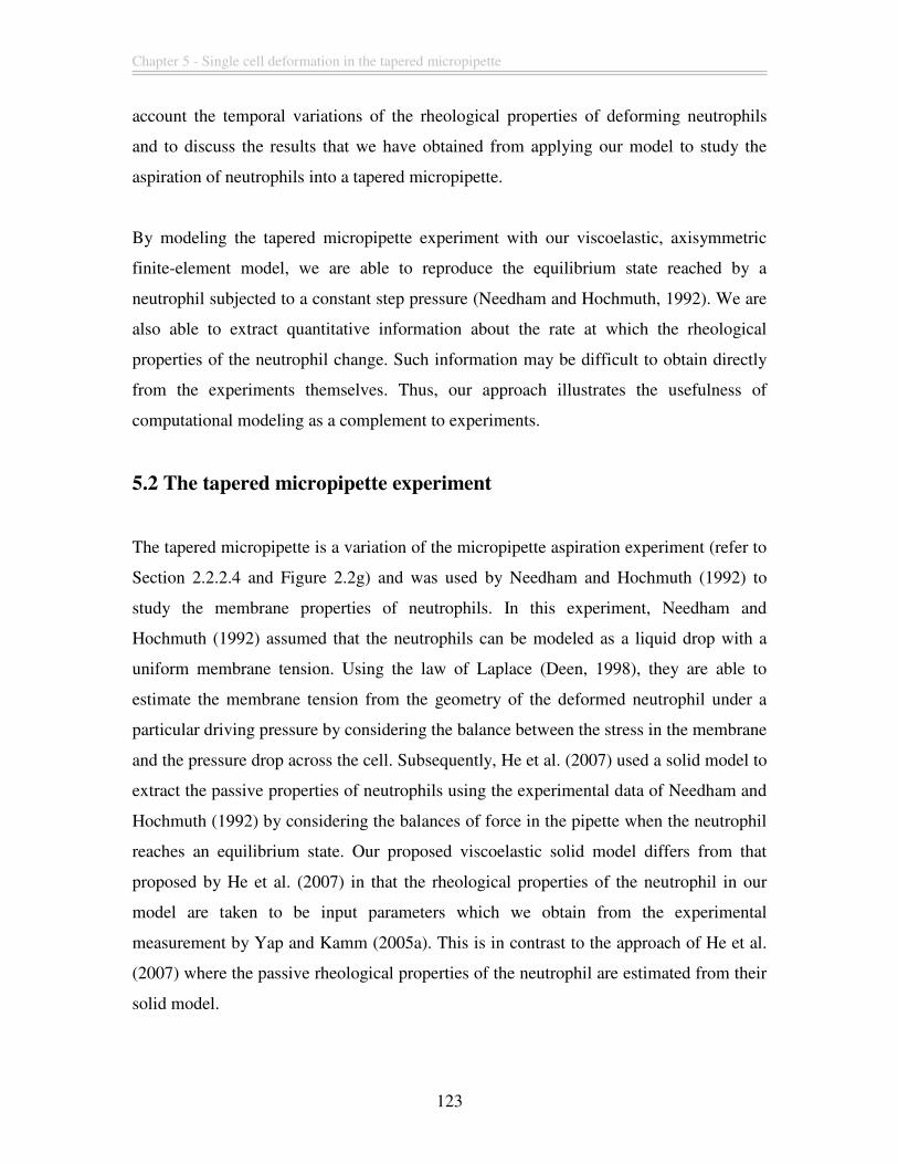
Chapter 5 - Single cell deformation in the tapered micropipette
123
account the temporal variations of the rheological properties of deforming neutrophils
and to discuss the results that we have obtained from applying our model to study the
aspiration of neutrophils into a tapered micropipette.
By modeling the tapered micropipette experiment with our viscoelastic, axisymmetric
finite-element model, we are able to reproduce the equilibrium state reached by a
neutrophil subjected to a constant step pressure (Needham and Hochmuth, 1992). We are
also able to extract quantitative information about the rate at which the rheological
properties of the neutrophil change. Such information may be difficult to obtain directly
from the experiments themselves. Thus, our approach illustrates the usefulness of
computational modeling as a complement to experiments.
5.2 The tapered micropipette experiment
The tapered micropipette is a variation of the micropipette aspiration experiment (refer to
Section 2.2.2.4 and Figure 2.2g) and was used by Needham and Hochmuth (1992) to
study the membrane properties of neutrophils. In this experiment, Needham and
Hochmuth (1992) assumed that the neutrophils can be modeled as a liquid drop with a
uniform membrane tension. Using the law of Laplace (Deen, 1998), they are able to
estimate the membrane tension from the geometry of the deformed neutrophil under a
particular driving pressure by considering the balance between the stress in the membrane
and the pressure drop across the cell. Subsequently, He et al. (2007) used a solid model to
extract the passive properties of neutrophils using the experimental data of Needham and
Hochmuth (1992) by considering the balances of force in the pipette when the neutrophil
reaches an equilibrium state. Our proposed viscoelastic solid model differs from that
proposed by He et al. (2007) in that the rheological properties of the neutrophil in our
model are taken to be input parameters which we obtain from the experimental
measurement by Yap and Kamm (2005a). This is in contrast to the approach of He et al.
(2007) where the passive rheological properties of the neutrophil are estimated from their
solid model.
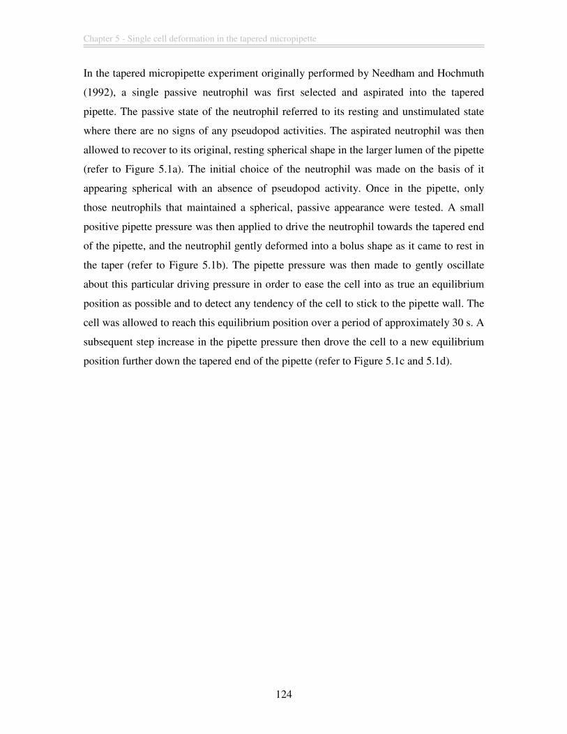
Chapter 5 - Single cell deformation in the tapered micropipette
124
In the tapered micropipette experiment originally performed by Needham and Hochmuth
(1992), a single passive neutrophil was first selected and aspirated into the tapered
pipette. The passive state of the neutrophil referred to its resting and unstimulated state
where there are no signs of any pseudopod activities. The aspirated neutrophil was then
allowed to recover to its original, resting spherical shape in the larger lumen of the pipette
(refer to Figure 5.1a). The initial choice of the neutrophil was made on the basis of it
appearing spherical with an absence of pseudopod activity. Once in the pipette, only
those neutrophils that maintained a spherical, passive appearance were tested. A small
positive pipette pressure was then applied to drive the neutrophil towards the tapered end
of the pipette, and the neutrophil gently deformed into a bolus shape as it came to rest in
the taper (refer to Figure 5.1b). The pipette pressure was then made to gently oscillate
about this particular driving pressure in order to ease the cell into as true an equilibrium
position as possible and to detect any tendency of the cell to stick to the pipette wall. The
cell was allowed to reach this equilibrium position over a period of approximately 30 s. A
subsequent step increase in the pipette pressure then drove the cell to a new equilibrium
position further down the tapered end of the pipette (refer to Figure 5.1c and 5.1d).
Chapter 5 - Single cell deformation in the tapered micropipette
125
Figure 5.1: Videomicrograph of the tapered micropipette experimental measurements. (a) ∆P = 0
dyn/cm2: a single passive cell was selected and aspirated into the tapered pipette and allowed to
recover to its resting spherical shape in the larger lumen of the pipette. (b) ∆P = 25 dyn/cm2: a
small positive pipette pressure was then applied and the cell was very gently deformed into a
bolus shape as it was driven down the pipette; it then came to rest in the taper. (c) ∆P = 50
dyn/cm2 and (d) ∆P = 75 dyn/cm2: step increases in pipette pressure then drove the cell to new
equilibrium positions. (Figure reproduced from Needham and Hochmuth, 1992.)
Chapter 5 - Single cell deformation in the tapered micropipette
126
5.3 Finite-element formulation
We use an axisymmetric formulation which allows us to capture the three dimensional
response of the cell in the tapered micropipette with a two dimensional model (similar to
the approach used in Chapter 4.2 for modeling the optical stretcher experiments). In this
chapter, the main difference is that we will assume that every discretized region within
the cell is represented by a viscoelastic Kelvin-Voigt (K-V) model (refer to Section 3.4
and Figure 3.14) consisting of a single spring element in parallel connection with a
dashpot element. The implementation of the finite element method for this chapter is
described in Section 3.4.2.
The choice of using a viscoelastic solid model is motivated by the experimental
observation that passive neutrophils reach an equilibrium state of a bolus shape in the
tapered micropipette for a constant driving pressure over a time period of about 30
seconds (refer to Figure 5.1). We also observe that the neutrophil is driven to a new
equilibrium position if a step increase in the driving pressure is applied after the original
equilibrium position is reached and that it does not deform indefinitely under a constant
driving pressure.
5.3.1 Model parameters
We note that the tapered micropipette experiment by Needham and Hochmuth (1992)
was conducted with the neutrophils being manipulated at room temperature. Thus, we
have decided to use the rheological properties of passive neutrophils measured
experimentally at 23 degrees Celsius (~room temperature) as reported by Yap and Kamm
(2005a) in our finite element model to simulate the conditions in the tapered micropipette
experiment. The experimental measurements of passive neutrophil rheological properties
and the corresponding parameters used for our finite element model are summarized in
Table 5.1:
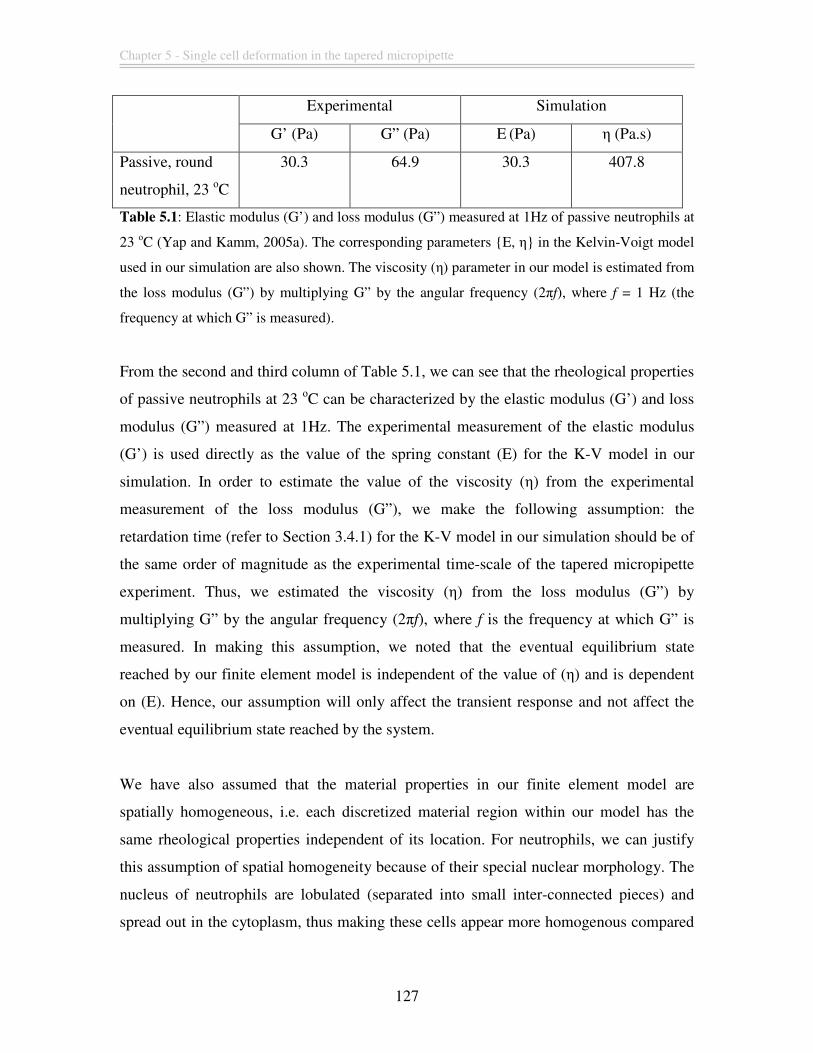
Chapter 5 - Single cell deformation in the tapered micropipette
127
Experimental Simulation
G’ (Pa) G” (Pa) E (Pa) η (Pa.s)
Passive, round
neutrophil, 23 οC
30.3 64.9 30.3 407.8
Table 5.1: Elastic modulus (G’) and loss modulus (G”) measured at 1Hz of passive neutrophils at
23 οC (Yap and Kamm, 2005a). The corresponding parameters {E, η} in the Kelvin-Voigt model
used in our simulation are also shown. The viscosity (η) parameter in our model is estimated from
the loss modulus (G”) by multiplying G” by the angular frequency (2πf), where f = 1 Hz (the
frequency at which G” is measured).
From the second and third column of Table 5.1, we can see that the rheological properties
of passive neutrophils at 23 οC can be characterized by the elastic modulus (G’) and loss
modulus (G”) measured at 1Hz. The experimental measurement of the elastic modulus
(G’) is used directly as the value of the spring constant (E) for the K-V model in our
simulation. In order to estimate the value of the viscosity (η) from the experimental
measurement of the loss modulus (G”), we make the following assumption: the
retardation time (refer to Section 3.4.1) for the K-V model in our simulation should be of
the same order of magnitude as the experimental time-scale of the tapered micropipette
experiment. Thus, we estimated the viscosity (η) from the loss modulus (G”) by
multiplying G” by the angular frequency (2πf), where f is the frequency at which G” is
measured. In making this assumption, we noted that the eventual equilibrium state
reached by our finite element model is independent of the value of (η) and is dependent
on (E). Hence, our assumption will only affect the transient response and not affect the
eventual equilibrium state reached by the system.
We have also assumed that the material properties in our finite element model are
spatially homogeneous, i.e. each discretized material region within our model has the
same rheological properties independent of its location. For neutrophils, we can justify
this assumption of spatial homogeneity because of their special nuclear morphology. The
nucleus of neutrophils are lobulated (separated into small inter-connected pieces) and
spread out in the cytoplasm, thus making these cells appear more homogenous compared
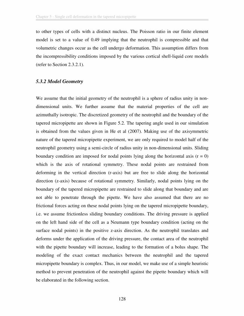
Chapter 5 - Single cell deformation in the tapered micropipette
128
to other types of cells with a distinct nucleus. The Poisson ratio in our finite element
model is set to a value of 0.49 implying that the neutrophil is compressible and that
volumetric changes occur as the cell undergo deformation. This assumption differs from
the incompressibility conditions imposed by the various cortical shell-liquid core models
(refer to Section 2.3.2.1).
5.3.2 Model Geometry
We assume that the initial geometry of the neutrophil is a sphere of radius unity in non-
dimensional units. We further assume that the material properties of the cell are
azimuthally isotropic. The discretized geometry of the neutrophil and the boundary of the
tapered micropipette are shown in Figure 5.2. The tapering angle used in our simulation
is obtained from the values given in He et al (2007). Making use of the axisymmetric
nature of the tapered micropipette experiment, we are only required to model half of the
neutrophil geometry using a semi-circle of radius unity in non-dimensional units. Sliding
boundary condition are imposed for nodal points lying along the horizontal axis (r = 0)
which is the axis of rotational symmetry. These nodal points are restrained from
deforming in the vertical direction (r-axis) but are free to slide along the horizontal
direction (z-axis) because of rotational symmetry. Similarly, nodal points lying on the
boundary of the tapered micropipette are restrained to slide along that boundary and are
not able to penetrate through the pipette. We have also assumed that there are no
frictional forces acting on these nodal points lying on the tapered micropipette boundary,
i.e. we assume frictionless sliding boundary conditions. The driving pressure is applied
on the left hand side of the cell as a Neumann type boundary condition (acting on the
surface nodal points) in the positive z-axis direction. As the neutrophil translates and
deforms under the application of the driving pressure, the contact area of the neutrophil
with the pipette boundary will increase, leading to the formation of a bolus shape. The
modeling of the exact contact mechanics between the neutrophil and the tapered
micropipette boundary is complex. Thus, in our model, we make use of a simple heuristic
method to prevent penetration of the neutrophil against the pipette boundary which will
be elaborated in the following section.
Chapter 5 - Single cell deformation in the tapered micropipette
129
5.3.3 Contact Heuristics
This section describes the contact heuristics that we have implemented in our viscoelastic
finite element model for the tapered micropipette experiment. We note that the
boundaries of the tapered micropipette are rigid and the nodal points representing the
material points of the neutrophils are not allowed to penetrate through this rigid surface.
In our simulation, this constraint is imposed primarily through the application of the
Lagrange multiplier technique for nodal points in contact with the inclined boundary of
the pipette. The nodal points in contact with the inclined boundary of the pipette are
constrained to slide frictionlessly along the boundary (refer to Figure 5.3a). However, as
the neturophil deforms under the application of the driving pressure, we note that nodal
points previously not in contact with the pipette boundary can come into contact or
penetrate through this surface (refer to Figure 5.3b). These occurrences of nodal point
penetrations are checked at the end of every time-step in our model and we used
sufficiently small time-step in our simulation to minimize the number of nodal points
penetrating through the pipette boundary (if such penetration occurs and to minimize the
extent of the penetration).
When such instances of penetrations occur, we first compute the shortest distance from
the penetrating nodal points to the inclined boundary and subsequently project these
penetrating nodal points back onto the boundary. We carried out this projection step by
imposing a Dirichlet displacement boundary condition on the affected nodal points while
allowing the remaining nodal points to freely deform (under no external loading but
subjected to the relevant boundary conditions). This projection step, done at the end of
the time-step, will affect the deformation of all the other nodal points. The aim is to
compute a deformation configuration that satisfies the boundary condition of non-
penetration of nodal points against the pipette boundary and balance the internal body
stress with the external applied stress for that particular time-step. For the subsequent
time-steps, we will update the boundary conditions for those nodal points that we had
projected previously onto the pipette boundary such that these nodal points are now only
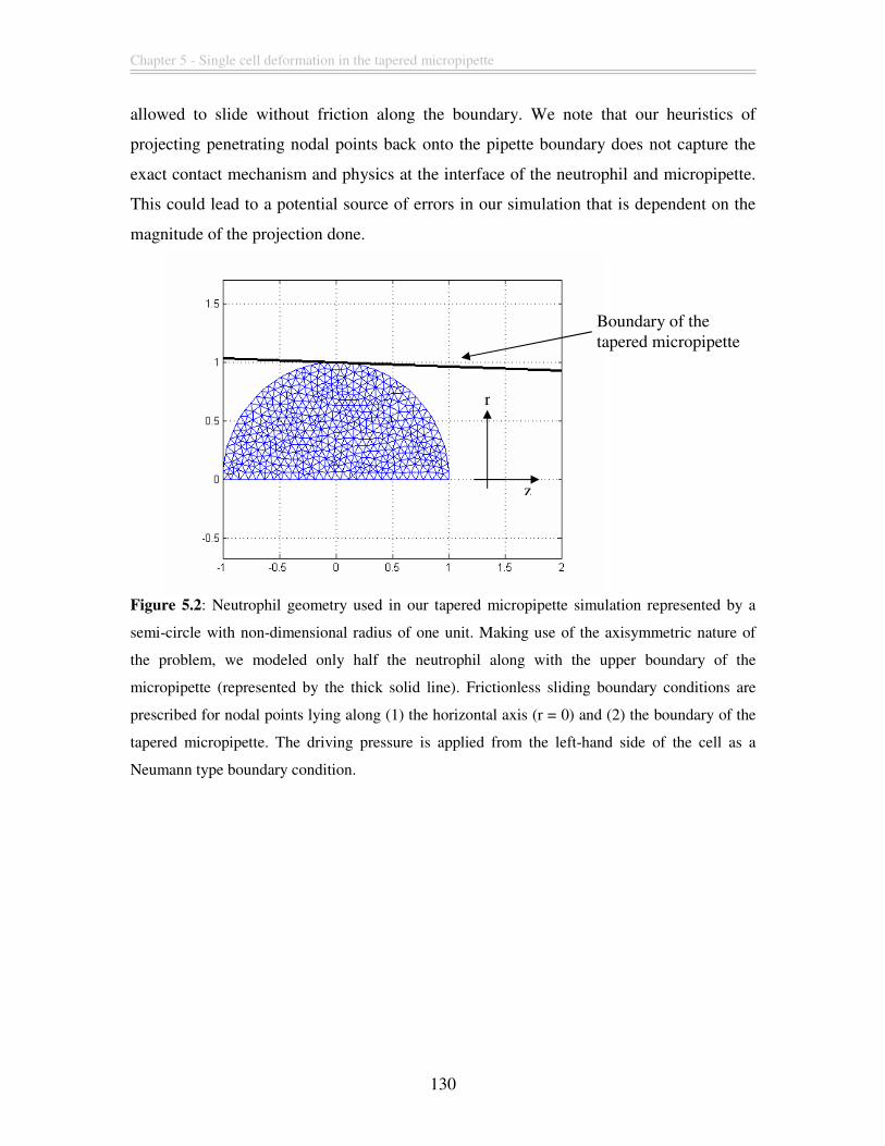
Chapter 5 - Single cell deformation in the tapered micropipette
130
allowed to slide without friction along the boundary. We note that our heuristics of
projecting penetrating nodal points back onto the pipette boundary does not capture the
exact contact mechanism and physics at the interface of the neutrophil and micropipette.
This could lead to a potential source of errors in our simulation that is dependent on the
magnitude of the projection done.
Figure 5.2: Neutrophil geometry used in our tapered micropipette simulation represented by a
semi-circle with non-dimensional radius of one unit. Making use of the axisymmetric nature of
the problem, we modeled only half the neutrophil along with the upper boundary of the
micropipette (represented by the thick solid line). Frictionless sliding boundary conditions are
prescribed for nodal points lying along (1) the horizontal axis (r = 0) and (2) the boundary of the
tapered micropipette. The driving pressure is applied from the left-hand side of the cell as a
Neumann type boundary condition.
Boundary of the tapered micropipette
r
z
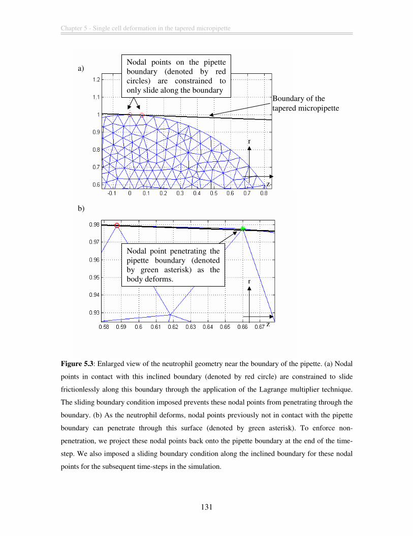
Chapter 5 - Single cell deformation in the tapered micropipette
131
Figure 5.3: Enlarged view of the neutrophil geometry near the boundary of the pipette. (a) Nodal
points in contact with this inclined boundary (denoted by red circle) are constrained to slide
frictionlessly along this boundary through the application of the Lagrange multiplier technique.
The sliding boundary condition imposed prevents these nodal points from penetrating through the
boundary. (b) As the neutrophil deforms, nodal points previously not in contact with the pipette
boundary can penetrate through this surface (denoted by green asterisk). To enforce non-
penetration, we project these nodal points back onto the pipette boundary at the end of the time-
step. We also imposed a sliding boundary condition along the inclined boundary for these nodal
points for the subsequent time-steps in the simulation.
r
z
Boundary of the tapered micropipette
a) Nodal points on the pipette boundary (denoted by red circles) are constrained to only slide along the boundary
b)
Nodal point penetrating the pipette boundary (denoted by green asterisk) as the body deforms. r
z
Chapter 5 - Single cell deformation in the tapered micropipette
132
5.4 Results
5.4.1 Temporal variation of neutrophil rheological properties provides better fit
to experimental data.
To model the tapered micropipette experiment, we run our simulation using the passive
neutrophil rheological properties measured at 23 οC (Yap and Kamm, 2005a, refer to
Table 5.1) for three different values of driving pressure i.e. ∆P = 25 dyn/cm2, 50 dyn/cm2
and 75 dyn/cm2. We will refer to these results as results obtained using the passive
model. For ∆P = 25 dyn/cm2, we run our simulation corresponding to the experimental
time duration of approximately 30 seconds, the time when the aspirated neutrophil
reaches an equilibrium state. For the other two values of driving pressure (∆P), we
applied an initial ∆P = 25 dyn/cm2 for 30 seconds (allowing the neutrophil to reach an
initial equilibrium state) before applying a step increase in the driving pressure to deform
the neutrophil into a new equilibrium state (which we assumed to take place over 30
seconds) in accordance to the experimental protocol outlined by Needham and Hochmuth
(1992). The variations of the driving pressure with respect to time are summarized in
Figure 5.4. From our simulation, we are able to extract both the displacement and
deformed length of the neutrophil (refer to Figure 5.5) and we compared our simulation
results to the experimental data based on the tapered micropipette experiment (Needham
and Hochmuth, 1992) that are estimated by He et al. (2007). These comparisons are
shown in Table 5.2. We have also plotted the deformed shaped of the neutrophil in the
tapered micropipette obtained from our simulation using the passive finite element model
in Figure 5.6. Comparing our simulation results in Figure 5.6 with the experimental
videomicrograph in Figure 5.1, we can see that our passive finite element model is able to
capture the qualitative response of the neutrophil with reasonable accuracy.
From Table 5.2, we can see that the fit to the experimental observation obtained using the
passive model is reasonable with percentage errors ranging from 5% to 10%. This allows
us to be reasonably confident that the assumptions made about the spatially homogeneity
of the rheological properties in our model is valid and we are able to capture the
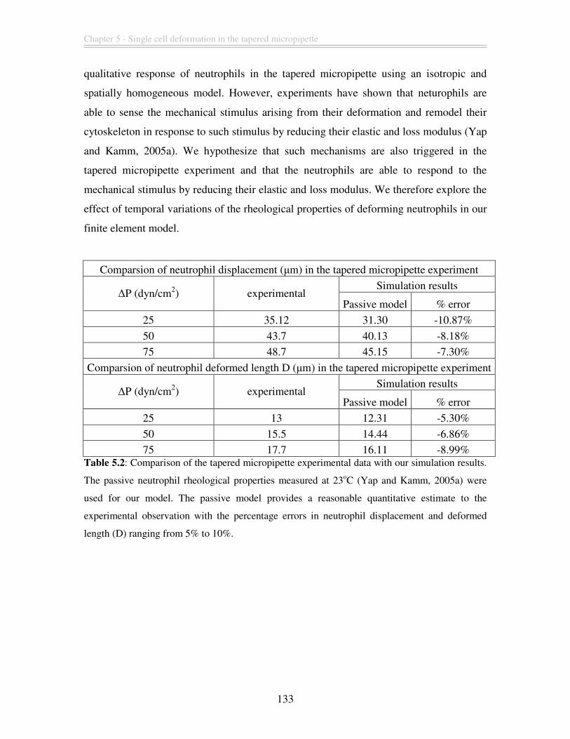
Chapter 5 - Single cell deformation in the tapered micropipette
133
qualitative response of neutrophils in the tapered micropipette using an isotropic and
spatially homogeneous model. However, experiments have shown that neturophils are
able to sense the mechanical stimulus arising from their deformation and remodel their
cytoskeleton in response to such stimulus by reducing their elastic and loss modulus (Yap
and Kamm, 2005a). We hypothesize that such mechanisms are also triggered in the
tapered micropipette experiment and that the neutrophils are able to respond to the
mechanical stimulus by reducing their elastic and loss modulus. We therefore explore the
effect of temporal variations of the rheological properties of deforming neutrophils in our
finite element model.
Comparsion of neutrophil displacement (µm) in the tapered micropipette experiment
Simulation results ∆P (dyn/cm2) experimental
Passive model % error
25 35.12 31.30 -10.87%
50 43.7 40.13 -8.18%
75 48.7 45.15 -7.30%
Comparsion of neutrophil deformed length D (µm) in the tapered micropipette experiment
Simulation results ∆P (dyn/cm2) experimental
Passive model % error
25 13 12.31 -5.30%
50 15.5 14.44 -6.86%
75 17.7 16.11 -8.99% Table 5.2: Comparison of the tapered micropipette experimental data with our simulation results.
The passive neutrophil rheological properties measured at 23oC (Yap and Kamm, 2005a) were
used for our model. The passive model provides a reasonable quantitative estimate to the
experimental observation with the percentage errors in neutrophil displacement and deformed
length (D) ranging from 5% to 10%.
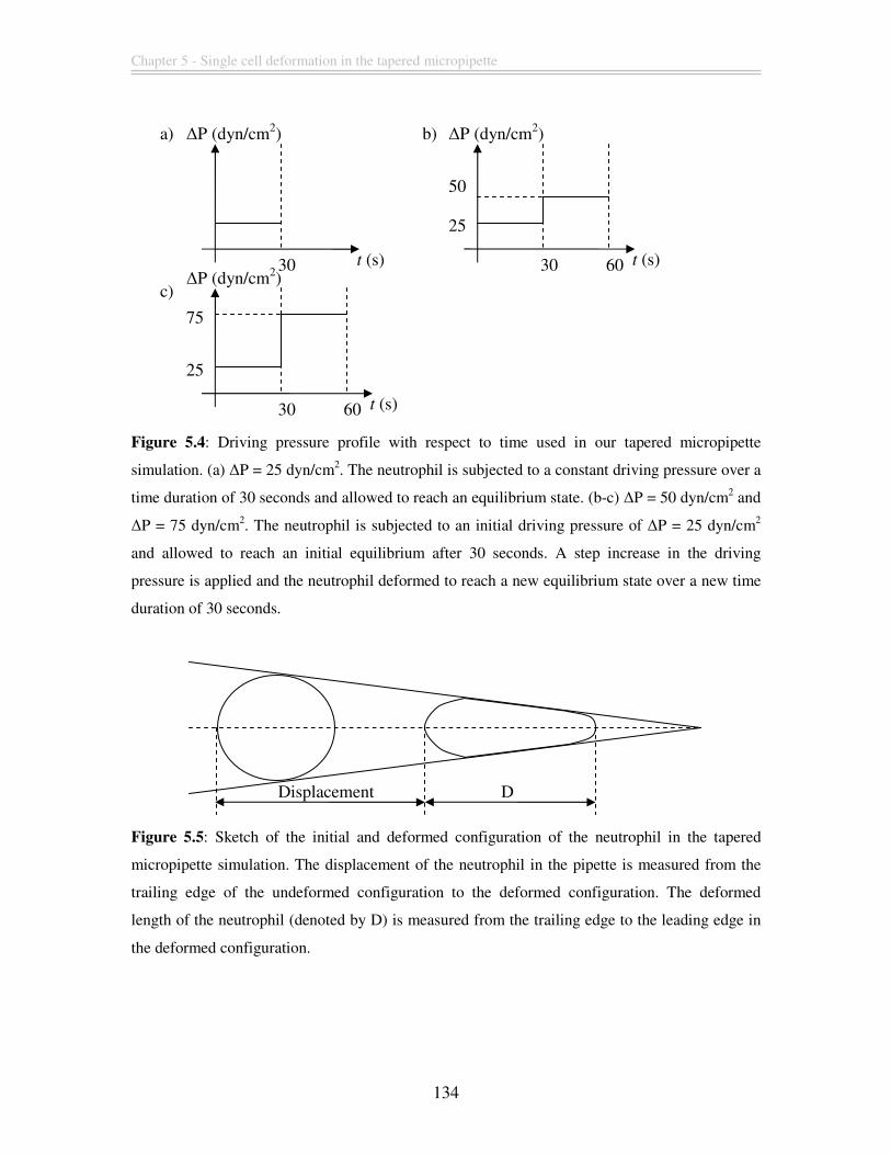
Chapter 5 - Single cell deformation in the tapered micropipette
134
Figure 5.4: Driving pressure profile with respect to time used in our tapered micropipette
simulation. (a) ∆P = 25 dyn/cm2. The neutrophil is subjected to a constant driving pressure over a
time duration of 30 seconds and allowed to reach an equilibrium state. (b-c) ∆P = 50 dyn/cm2 and
∆P = 75 dyn/cm2. The neutrophil is subjected to an initial driving pressure of ∆P = 25 dyn/cm2
and allowed to reach an initial equilibrium after 30 seconds. A step increase in the driving
pressure is applied and the neutrophil deformed to reach a new equilibrium state over a new time
duration of 30 seconds.
Figure 5.5: Sketch of the initial and deformed configuration of the neutrophil in the tapered
micropipette simulation. The displacement of the neutrophil in the pipette is measured from the
trailing edge of the undeformed configuration to the deformed configuration. The deformed
length of the neutrophil (denoted by D) is measured from the trailing edge to the leading edge in
the deformed configuration.
∆P (dyn/cm2)
t (s)
30
∆P (dyn/cm2)
t (s)
25
30
50
60 ∆P (dyn/cm2)
t (s)
25
30
75
60
a) b)
c)
Displacement D
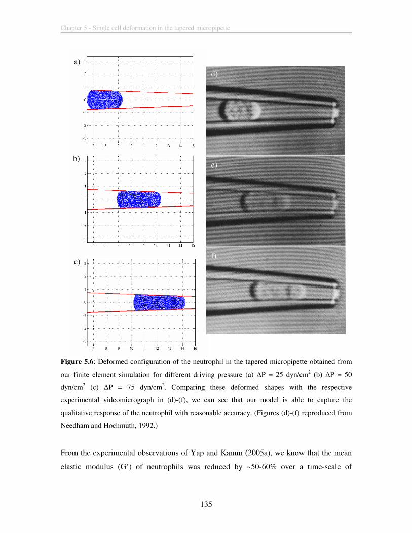
Chapter 5 - Single cell deformation in the tapered micropipette
135
Figure 5.6: Deformed configuration of the neutrophil in the tapered micropipette obtained from
our finite element simulation for different driving pressure (a) ∆P = 25 dyn/cm2 (b) ∆P = 50
dyn/cm2 (c) ∆P = 75 dyn/cm2. Comparing these deformed shapes with the respective
experimental videomicrograph in (d)-(f), we can see that our model is able to capture the
qualitative response of the neutrophil with reasonable accuracy. (Figures (d)-(f) reproduced from
Needham and Hochmuth, 1992.)
From the experimental observations of Yap and Kamm (2005a), we know that the mean
elastic modulus (G’) of neutrophils was reduced by ~50-60% over a time-scale of
a)
b)
c)
d)
e)
f)
Chapter 5 - Single cell deformation in the tapered micropipette
136
between 10 to 20 seconds. Similarly, the mean loss modulus (G”) was reduced by ~35-
50% over the same time-scale. These reductions in the elastic and loss modulus were
maintained until pseudopod projections appeared and the time required for pseudopod
projections appears to be inversely correlated to the rate of neutrophil deformation. We
note that the experiments of Yap and Kamm (2005a) were carried out at 37oC but we
assumed that the mechanism governing the reduction in the elastic and loss modulus
upon neutrophil deformation is temperature independent. Thus, we would still be able to
use the trend reported by Yap and Kamm for our temporal finite element model of the
tapered micropipette experiment.
Using the rheological properties of neutrophil measured at 23oC (Yap and Kamm, 2005a)
as the baseline value, the elastic modulus (G’) and the loss modulus (G”) of our tapered
micropipette model is reduced by 50% and 35% respectively based on the trend reported
by Yap and Kamm. We assumed that this reduction takes places over a time-scale of
approximately 10 seconds after application of the driving pressure that deforms the
neutrophil based on the experimental observation of Yap and Kamm. In our temporal
variation model, we denoted this time-scale over which this reduction in the elastic and
loss moduli occurs as τ. We also assumed that this reduction of the elastic and loss
modulus follows a linear trend from time t = 0 to time t = τ, and that the rheological
properties of the neutrophil is maintained at these reduced values for the remaining
duration of the simulation (for τ ≤ t ≤ 60). We further assumed that the subsequent
increase in driving pressure (for the case of ∆P = 50 dyn/cm2 and ∆P = 75 dyn/cm2) does
not lead to any further reduction in the rheological properties of the neutrophil. The
temporal variation in the elastic modulus and loss modulus are summarized in Figure 5.7.
The results of our simulation for incorporating this temporal variation in the elastic
modulus (G’) and loss modulus (G”) for value of τ = 10s are compared to the passive
model in Table 5.3. From Table 5.3, we can see that our temporal variation model (cells
highlighted in grey) provides a better quantitative estimate to the tapered micropipette
experimental data when compared to the passive model. The percentage errors in the
neutrophil displacement and deformed length (D) obtained using the temporal variation
model range from 0.3% to 5% which is a reasonable improvement over the passive
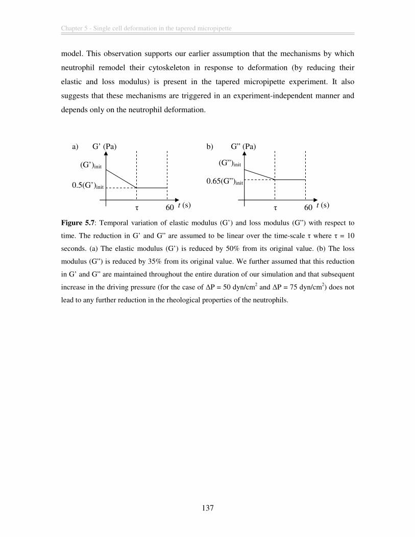
Chapter 5 - Single cell deformation in the tapered micropipette
137
model. This observation supports our earlier assumption that the mechanisms by which
neutrophil remodel their cytoskeleton in response to deformation (by reducing their
elastic and loss modulus) is present in the tapered micropipette experiment. It also
suggests that these mechanisms are triggered in an experiment-independent manner and
depends only on the neutrophil deformation.
Figure 5.7: Temporal variation of elastic modulus (G’) and loss modulus (G”) with respect to
time. The reduction in G’ and G” are assumed to be linear over the time-scale τ where τ = 10
seconds. (a) The elastic modulus (G’) is reduced by 50% from its original value. (b) The loss
modulus (G”) is reduced by 35% from its original value. We further assumed that this reduction
in G’ and G” are maintained throughout the entire duration of our simulation and that subsequent
increase in the driving pressure (for the case of ∆P = 50 dyn/cm2 and ∆P = 75 dyn/cm2) does not
lead to any further reduction in the rheological properties of the neutrophils.
G’ (Pa)
t (s)
τ
(G’)init
60
0.5(G’)init
(G”)init
0.65(G”)init
G” (Pa)
t (s)
τ 60
a) b)
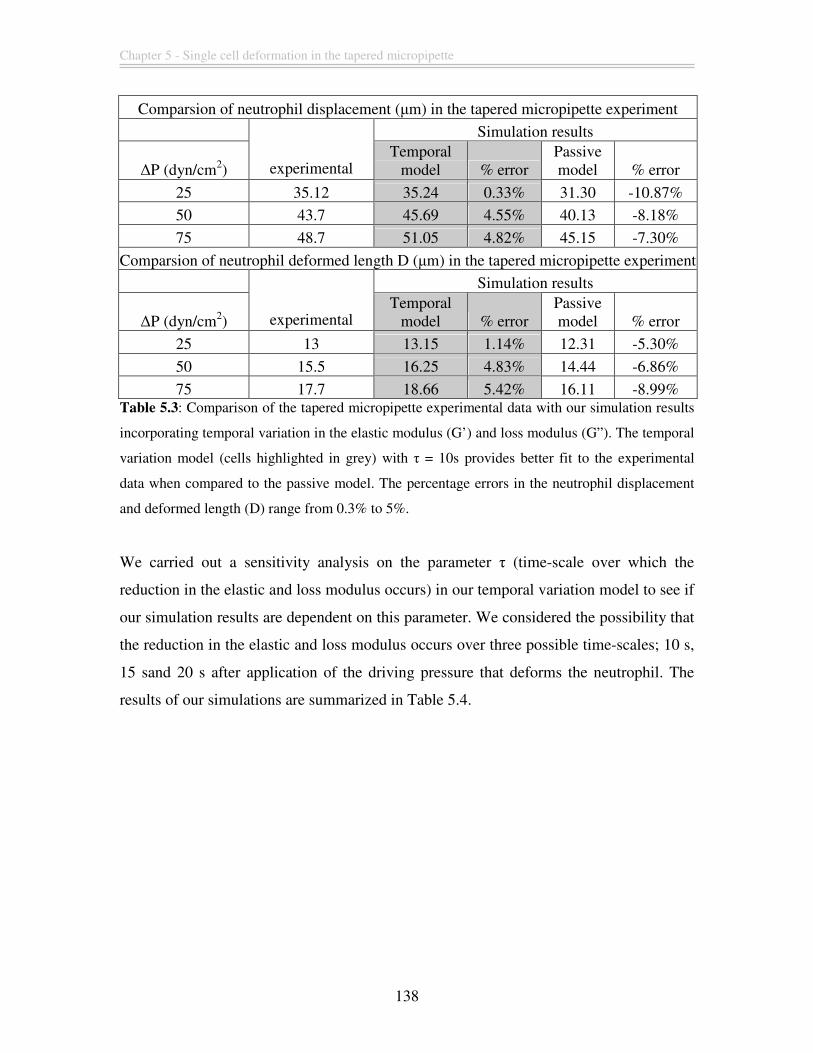
Chapter 5 - Single cell deformation in the tapered micropipette
138
Comparsion of neutrophil displacement (µm) in the tapered micropipette experiment
Simulation results
∆P (dyn/cm2) experimental Temporal
model % error Passive model % error
25 35.12 35.24 0.33% 31.30 -10.87%
50 43.7 45.69 4.55% 40.13 -8.18%
75 48.7 51.05 4.82% 45.15 -7.30%
Comparsion of neutrophil deformed length D (µm) in the tapered micropipette experiment
Simulation results
∆P (dyn/cm2) experimental Temporal
model % error Passive model % error
25 13 13.15 1.14% 12.31 -5.30%
50 15.5 16.25 4.83% 14.44 -6.86%
75 17.7 18.66 5.42% 16.11 -8.99% Table 5.3: Comparison of the tapered micropipette experimental data with our simulation results
incorporating temporal variation in the elastic modulus (G’) and loss modulus (G”). The temporal
variation model (cells highlighted in grey) with τ = 10s provides better fit to the experimental
data when compared to the passive model. The percentage errors in the neutrophil displacement
and deformed length (D) range from 0.3% to 5%.
We carried out a sensitivity analysis on the parameter τ (time-scale over which the
reduction in the elastic and loss modulus occurs) in our temporal variation model to see if
our simulation results are dependent on this parameter. We considered the possibility that
the reduction in the elastic and loss modulus occurs over three possible time-scales; 10 s,
15 sand 20 s after application of the driving pressure that deforms the neutrophil. The
results of our simulations are summarized in Table 5.4.
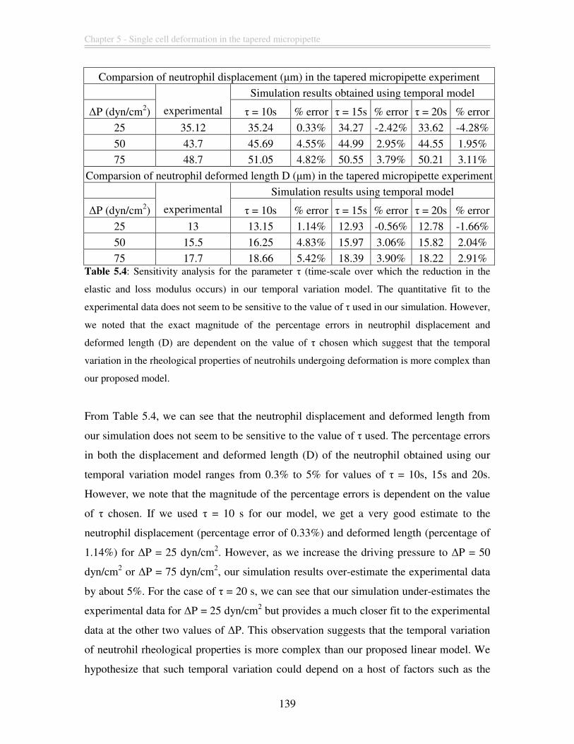
Chapter 5 - Single cell deformation in the tapered micropipette
139
Comparsion of neutrophil displacement (µm) in the tapered micropipette experiment
Simulation results obtained using temporal model
∆P (dyn/cm2) experimental τ = 10s % error τ = 15s % error τ = 20s % error
25 35.12 35.24 0.33% 34.27 -2.42% 33.62 -4.28%
50 43.7 45.69 4.55% 44.99 2.95% 44.55 1.95%
75 48.7 51.05 4.82% 50.55 3.79% 50.21 3.11%
Comparsion of neutrophil deformed length D (µm) in the tapered micropipette experiment
Simulation results using temporal model
∆P (dyn/cm2) experimental τ = 10s % error τ = 15s % error τ = 20s % error
25 13 13.15 1.14% 12.93 -0.56% 12.78 -1.66%
50 15.5 16.25 4.83% 15.97 3.06% 15.82 2.04%
75 17.7 18.66 5.42% 18.39 3.90% 18.22 2.91% Table 5.4: Sensitivity analysis for the parameter τ (time-scale over which the reduction in the
elastic and loss modulus occurs) in our temporal variation model. The quantitative fit to the
experimental data does not seem to be sensitive to the value of τ used in our simulation. However,
we noted that the exact magnitude of the percentage errors in neutrophil displacement and
deformed length (D) are dependent on the value of τ chosen which suggest that the temporal
variation in the rheological properties of neutrohils undergoing deformation is more complex than
our proposed model.
From Table 5.4, we can see that the neutrophil displacement and deformed length from
our simulation does not seem to be sensitive to the value of τ used. The percentage errors
in both the displacement and deformed length (D) of the neutrophil obtained using our
temporal variation model ranges from 0.3% to 5% for values of τ = 10s, 15s and 20s.
However, we note that the magnitude of the percentage errors is dependent on the value
of τ chosen. If we used τ = 10 s for our model, we get a very good estimate to the
neutrophil displacement (percentage error of 0.33%) and deformed length (percentage of
1.14%) for ∆P = 25 dyn/cm2. However, as we increase the driving pressure to ∆P = 50
dyn/cm2 or ∆P = 75 dyn/cm2, our simulation results over-estimate the experimental data
by about 5%. For the case of τ = 20 s, we can see that our simulation under-estimates the
experimental data for ∆P = 25 dyn/cm2 but provides a much closer fit to the experimental
data at the other two values of ∆P. This observation suggests that the temporal variation
of neutrohil rheological properties is more complex than our proposed linear model. We
hypothesize that such temporal variation could depend on a host of factors such as the
Chapter 5 - Single cell deformation in the tapered micropipette
140
magnitude and rate of the cellular deformation, nature and localization of the mechanical
stimulus etc. We also have not considered the possible recovery of the elastic and loss
modulus to their baseline values as the neutrophil reaches equilibrium state in the tapered
micropipette. This recovery response in the elastic and loss modulus was observed
experimentally by Yap and Kamm (2005a). However, the recovery response seems to be
sensitively dependent on the experimental conditions applied to the neutrophil in their
experiment and we believe that such responses are not generic in nature. Hence, our
model does not incorporate any recovery of the elastic and loss modulus to their baseline
values.
The improvement in our simulation results for the tapered micropipette experimental data
obtained using our temporal variation model as compared to the passive model rests upon
several assumptions made in the model formulation. The first assumption is that the
mechanism governing the reduction in both the elastic (G’) and loss modulus (G”) as
observed by Yap and Kamm (2005a) is temperature independent and is present in the
tapered micropipette experiment. As the setups of these two experiments are different and
the neutrophils are subjected to different temperature, it is conceivable that the trend of
the elastic and loss modulus reduction occurring in the tapered micropipette would be
different from that reported by Yap and Kamm (2005a). However, it is difficult to
postulate how such differences in the rheological response of the neutrophil would affect
our simulation results obtained using the temporal variation model without a-priori
knowledge of the effect of temperature on the elastic and loss modulus reduction. We
suggests that experiments be carried out to measure the elastic and loss modulus of
neutrophils aspirated into the tapered micropipette before application of suction pressure
and after the neturophils reach the equilibrium state. By conducting measurement of the
rheological properties at these two conditions, it would be possible to detect any such
reduction in the elastic and loss modulus and the rate of such reduction.
In our temporal variation model, we also assumed that the reductions in the elastic and
loss modulus follow a linear trend and that the subsequent increase in driving pressure
(from 25 dyn/cm2 to 50 dyn/cm2 or 75 dyn/cm2) does not trigger any further reduction in
Chapter 5 - Single cell deformation in the tapered micropipette
141
these moduli. From the experimental observations of Yap and Kamm (2005a), we know
that the elastic and loss modulus of the neutrophils measured prior to deformation and
during the period when the neutrophils are deformed inside the narrow channel showed a
reduction. As it is not possible to measure the rheological properties of the neutrohils
continuously in their experiments, the data presented in their paper showed the elastic
modulus and loss modulus before deformation into the narrow channel and at discrete
time interval after the deformation. The reductions in these moduli occurred over a time
scale of about 10 to 20 seconds. It is highly unlikely that the rheological properties of the
neutrophil changes in a stepwise manner. So the question remains on how we choose the
function to represent this reduction in our model? There are no obvious choices of
functions but we chose a linear response in our model for simplicity. We also
acknowledge that the subsequent increase in the driving pressure in the tapered
micropipette could also possibly trigger additional reduction in the rheological properties
of the neutrophils but it is difficult to know how the magnitude of such potential
reduction and its time scale varies without further experimental data.
We also note that our finite element model for the tapered micropipette is based on a
small strain formulation while the actual experimental setup involves neutrophils
undergoing large deformation, as evident from Figure 5.6. Thus, we would expect a
source of errors in our model arising from this geometrical non-linearity of large strain.
The comparison of the simulation results obtained using the passive and temporal
variation model should be viewed in light of our model limitation. It is possible that a
better fit to the tapered micropipette experimental data could be obtain using a passive
model, where the rheological properties remain constant in time, by incorporating large
strain formulation. We further note that the contact heuristic implemented in our model is
an approximation to the actual contact phenomenon occurring between the neutrophil and
the pipette wall and this represents another possible source of errors in our model.
Adopting a more detailed contact formulation, such as incorporating frictional forces
between the neutrophil and the pipette wall, could also improve the fit of the passive
model to the experimental data.
Chapter 5 - Single cell deformation in the tapered micropipette
142
Furthermore, the rheological properties used in our model are obtained from the
experiments conducted on neutrophils at 23 οC (Yap and Kamm, 2005a). Given that the
tapered micropipette experiment was conducted at room temperature (without actual
specification of the temperature), it is conceivable that slight changes to the rheological
properties of our passive model would allow us to obtain a better fit to the experimental
data. In addition, given the uncertainty and variability in the measurement of cellular
properties, it would not be surprising to expect some sources of errors in the experiments
conducted to measure the rheological properties of passive neutrophils. This translates
into some degrees of freedom for the material properties in our passive model. We have
not conducted a sensitivity analysis to see how the results obtained from our passive
model would change if we varied the material parameters used. It is quite likely that the
errors of the results obtained from our passive model could also be reduced in this
manner.
However, Yap and Kamm (2005a) have shown in their experiments that the rheological
properties of neutrophils change upon deformation in a temporal manner. While the exact
mechanisms of such changes are beyond the scope of our modeling effort, our main
objective is to investigate if incorporating such temporal variation into our model of the
tapered micropipette will give us better results as compared to the results obtained using a
passive model. Hence, despite the limitation and simplicity of our temporal variation
model, we have shown that the results obtained using such a model does fit better to the
experimental data as compared to a passive model. Furthermore, we reiterate that we are
able to reproduce the qualitative response of the neutrophil in the tapered micropipette
experiment, suggesting that neutrophils are capable of cellular remodeling upon
deformation in a wide variety of circumstances.
5.5. Conclusion
We have described a viscoelastic, axisymmetric finite-element model that takes into
account the temporal variation of rheological properties of neutrohpils and have shown
that our model can be used to simulate their response in the tapered micropipette
Chapter 5 - Single cell deformation in the tapered micropipette
143
experiment. The main result of this chapter is that the temporal variation model provides
a better fit to experimental data when compared to the passive model. Thus, our model
suggests that cellular remodeling, in the form of a decreased cellular viscoelasticity,
occurred during the process of neutrophil aspiration. We have shown that the percentage
errors in both the displacement and deformed length of the neutrophil obtained using our
temporal variation model are smaller than the passive neutrophil model. However, the
degree of fit is sensitively dependent on the driving pressure ∆P, and the parameter τ, the
time-scale over which the reduction in the elastic and loss modulus occurs. We
hypothesize that the temporal variation in the rheological properties of neutrohil is more
complex and could depend on a host of other factors. Despite the limitations and
simplicity of our model, we are able to capture the qualitative response of the neutrophil
in the tapered micropipette experiment, illustrating the usefulness of our model in
providing insights into the rheological responses of neutrophils under mechanical
deformation.
Chapter 6 - Conclusion and future work
144
Chapter 6. Conclusion and future work
In summary, we re-emphasize that the objective of this thesis is to apply computational
modeling to study the deformation transients of single cells under the influence of
mechanical stress. We have shown in Chapters 4 and 5 that the cellular deformation
measured experimentally can be adequately described using our finite element model that
incorporates both spatial and temporal variations to the material properties.
In particular, we have applied our viscoelastic, axisymmetric finite-element model in
Chapter 3 to simulate the stretching of suspended fibroblast cells in the optical stretcher,
taking into account the spatiotemporal heterogeneity of the cells. We have shown that
cellular remodeling, in the form of an increase in the cellular viscosity, is necessary in
order to fit our simulation results to the experimentally-observed strain development for
both 0.2 s and 2.5 s loading (Wottawah et al., 2005a). It is likely that the mechanism of
this cellular remodeling can be attributed to the heating effects induced by the optical
stretcher where the temperature increases approximately 30ºC within 0.2 s (Ebert et al.,
2007). Our simulations also suggest that the higher optical deformability observed for
malignant fibroblasts (Guck et al., 2005) can be explained by the difference in the surface
stretching profile (which is related to the cell size). The differences in the size between
the normal and malignant fibroblasts induce a different surface stretching profile in the
optical stretcher. From our model, we have shown that the effect of this difference in the
stretching profile is a more important factor in determining the radial deformation of the
fibroblast than the thickness of the actin cortical region. This suggests that fibroblasts
with a smaller radius will experience higher strain compared to fibroblasts with a larger
radius in the optical stretcher due to the stress profile experienced. The final result from
this chapter suggests that the modes of stress propagation into the cytoplasm are different
for normal and malignant fibroblasts. Our simulation shows that the Von Mises stress
distribution within the cell is dependent on the surface stretching profiles used. For the
localized stretching profile, the regions with the highest Von Mises stress concentration
are offset from the centre of the cell and occur at a region just beneath the cortical region.
Chapter 6 - Conclusion and future work
145
In Chapter 5, we applied our viscoelastic, axisymmetric finite-element model
incorporating temporal variation of rheological properties to simulate the deformation of
neutrophils in the tapered micropipette experiment. The main result of this chapter is that
the temporal variation model provides a better fit to experimental data when compared to
the passive model. We have shown that the percentage errors in both the displacement
and deformed length of the neutrophil obtained using our temporal variation model is
smaller compared to the passive neutrophil model. Our results suggest that neutrophils in
the tapered micropipette experiments undergo cellular remodeling upon deformation in a
similar manner as neutrophils deforming in a narrow channel (Yap and Kamm, 2005a).
Our simulation results suggest that cells are able to sense deformation and respond to
mechanical stimuli by varying their elasticity and viscosity temporally. We hypothesize
that such mechanisms are common across different cell types, though the exact nature of
the response (increase/decrease in cellular elasticity and/or viscosity) and the means in
which such responses are elicited are likely to be cell-type dependent. In particular, we
have shown using our simulation that suspended fibroblasts are able to increase their
cellular viscosity temporally in the optical stretcher while neutrophils are able to decrease
their cellular elasticity and viscosity temporally in the tapered micropipette experiment.
The difference in the response to mechanical stimuli for fibroblasts and neutrophils is
probably the result of the highly specialized functions performed by these two types of
cells. Fibroblasts are primarily found in connective tissue and are involved with the local
maintenance and repair of the extracellular fibers. In contrast, neutrophils are found in the
cardiovascular system and form an integral part of our immune system defense against
viruses and bacteria. Thus, we can see that these two types of cells perform very different
functions and roles. Despite these differences, our simulation results suggest that both
fibroblasts and neutrophils are capable of responding to deformation and mechanical
stimulus by changing their rheological properties in a temporal manner.
In this thesis, our focus has been on the effects of mechanical deformation on the
rheological properties of single cells. We have not considered the responses of cells in
multi-cellular systems. In order to model such multi-cellular systems, we will need to
Chapter 6 - Conclusion and future work
146
extend our finite element model to incorporate the issue of cell-cell and cell-ECM (extra-
cellular matrix) adhesion as well as the contact mechanism between the cell and its
surrounding. As an example, the cells within an epithelium adhere to each other and to
the ECM through specialized protein complexes. Cells are linked to other cells through
specialized complexes which fall into three classes: tight junctions, adherens junctions
and desmosomes (Alberts et al., 2002). The interaction between the cell and the ECM are
mediated either through specialized structures, known as hemidesmosomes, or through
direct interaction between specialized cell-surface proteins and components of the ECM.
One possible strategy is to develop a coarse-grained modeling approach that will allow us
to incorporate all these various interactions among the various protein complexes while
retaining essential and sufficient details on the adhesion strength. In addition, mechanical
stresses are not the only stimulus that cells experience in their native environment.
Biochemical signals play an integral role in mediating cellular response through a wide
range of signaling pathways. These signaling pathways can affect the rheological
properties of the cell and the cellular deformation can in turn affect the reaction rates of
these signaling pathways. Hence, it is essential that we consider such effects in our model
in order to obtain a more accurate description of the cellular processes occurring.
Nevertheless, we have shown in this thesis that our computational model can be used
successfully to investigate single cells deforming under the influence of mechanical
stresses.
References
147
References
Alberts, B., Johnson, A., Lewis, J., Raff, M., Roberts, K., Walter, P., 2002. Molecular
Biology of the Cell. 4th Edition. Garland Science, NY.
Ananthakrishnan, R., Guck, J., Wottawah, F., Schinkinger, S., Lincoln, B., Romeyke, M.,
Moon, T., Kas, J., 2006. Quantifying the contribution of actin networks to the elastic
strength of fibroblasts. Journal of Theoretical Biology 242, 502-516.
Bausch, A.R., Ziemann, F., Boulbitch, A.A., Jacobson, K., Sackmann, E., 1998. Local
Measurements of viscoelastic parameters of adherent cell surfaces by magnetic bead
microrheometry. Biophysical Journal 75, 2038–2049.
Bausch, A.R., Moller, W., Sackmann, E., 1999. Measurement of local viscoelasticity and
forces in living cells by magnetic tweezers. Biophysical Journal 76, 573-579.
Binnig, G., Quate, C.F., Gerber, C., 1986. Atomic force microscope. Physical Review
Letters 56, 930-933.
Boudreau, N., Bissell, M.J., 1998. Extracellular matrix signaling: integration of form and
function in normal and malignant cells. Current Opinion in Cell Biology 10, 640–646.
Caille, N., Thoumine, O., Tardy, Y., Meister, J.-J., 2002. Contribution of the nucleus to
the mechanical properties of endothelial cells. Journal of Biomechanics 35, 177-187.
Chen, C.S., Mrksich, M., Huang, S., Whitesides, G.M., Ingber, D.E., 1997. Geometric
Control of Cell Life and Death. Science 276, 1425–1428.
Cloitre, M., Borregam, R., Leibler, L., 2000. Rheological of aging and rejuvenation in
microgel pastes. Physical Review Letters 85, 4819-4822.
References
148
Cloitre, M., Borregam, R., Monti, F., Leibler, L., 2003. Glassy dynamics and flow
properties of soft colloidal pastes. Physical Review Letters 90, 68303.
Clough, R.W., 1960. The finite element method in plane stress analysis. Proceedings of
the American Society of Civil Engineers 23, 345-378.
Coughlin, M.F., Schmid-Schonbein, G.W., 2004. Pseudopod projection and cell
spreading of passive leukocytes in response to fluid shear stress. Biophysical Journal 87,
2035-2042.
Courant, R., 1943. Variational methods for the solution of problems of equilibrium and
vibrations. Bulletin of the American Mathematical Society 49, 1-23.
Dao, M., Lim, C.T., Suresh, S., 2003. Mechanics of the human red blood cell deformed
by optical tweezers. Journal of the Mechanics and Physics of Solids 51, 2259-2280.
de Pablo, P.J., Colchero, J., Gomez-Herrero, J., Baro, A.M., 1998. Jumping mode
scanning force microscopy. Applied Physics Letters 73, 3300-3302.
Deen, W.M., 1998. Analysis of Transport Phenomena. Oxford University Press, New
York.
Doerschuk, C.M., Beyers, N., Coxson, H.O., Wiggs, B., Hogg, J.C., 1993. Comparison of
neutrophil and capillary diameters and their relation to neutrophil sequestration in the
lung. Journal of Applied Physiology 74, 3040-3045.
Dong, C., Skalak, R., Sung, K.L., Schmid-Schonbein, G.W., Chien, S., 1988. Passive
deformation analysis of human leukocytes. Journal of Biomechanical Engineering 110,
27-36.
References
149
Dong, C., Skalak, R., Sung, K.L., 1991. Cytoplasmic rheology of passive neutrophils.
Biorheology 28, 557-567.
Dufrene, Y.F., 2003. Recent progress in the application of atomic force microscopy
imaging and force spectroscopy to microbiology. Current Opinion in Microbiology 6,
317-323.
Duszyk, M., Schwab, B.S., Zahalak, G.I., Qian, H., Elson, E.L., 1989. Cell poking:
Quantitative analysis of indentation of thick viscoelastic layers. Biophysical Journal 55,
683-690.
Ebert, S., Travis, K., Lincoln, B., Guck, J., 2007. Fluorescence ratio thermometry in a
microfluidic dual-beam laser trap. Optics Express 15, 15493-15499.
Eichinger, L., Koppel, B., Noegel, A.A., Schleicher, M., Schliwa, M., Weijer, K., Witke,
W., Janmey, P.A., 1996. Mechanical perturbation elicits a phenotypic difference between
Dictyostelium wild-type cells and cytoskeletal mutants. Biophysical Journal 70, 1054-
1060.
Evans, E., Kukan, B., 1984. Passive material behavior of granulocytes based on large
deformation and recovery after deformation tests. Blood 64, 1028-1035.
Evans, E., 1989. Structure and deformation properties of red blood cells: Concept and
Quantitative methods. Methods in Enzymology 173, 3-35.
Fabry, B., Maksym, G.N., Butler, J.P., Glogauer, M., Navajas, D., Fredberg, J.J., 2001.
Scaling the Microrheology of Living Cells. Physical Review Letters 87, 148102
Findley, W.N., Lai, J.S., Onaran, K., 1976. Creep and relaxation of non-linear
viscoelastic materials, with an introduction to linear viscoelasticity. North-Holland Pub.
Co., Amsterdam.
References
150
Fung, Y.C., 1965. Foundations of Solid Mechanics. Prentice-Hall Inc., Englewood Cliffs,
NJ.
Fung, Y.C., Tong, P., 2001. Advanced Series in Engineering Science - Volume 1:
Classical and computational solid mechanics. World Scientific, Singapore
Gardel, M.L., Shin, J.H., Mackintosh, F.C., Mahadevan, L., Matsudaira, P., Weitz, D.A.,
2004. Elastic behavior of cross-linked and bundled actin networks. Science 304, 1301-
1305.
Gardel, M.L., Nakamura, F., Hartwig, J., Crocker, J.C., Stossel, T.P., Weitz, D.A., 2006.
Stress-dependent elasticity of composite actin networks as a model for cell behaviour.
Physical Review Letters 96, 088102.
Gebb, S.A., Graham, J.A., Hanger, C.C., Godbey, P.S., Capen, R.L., Doerschuk, C.M.,
Wagner, W.W., 1995. Sites of leukocyte sequestration in the pulmonary microcirculation.
Journal of Applied Physiology 79, 493-497.
Giddens, D.P., Zarins, C.K., Glagov, S., 1993. The role of fluid mechanics in the
localization and detection of atherosclerosis. Journal of biomechanical engineering 115,
588-594.
Guck, J., Ananthakrishnan, R, Moon, T.J., Cunningham, C.C., Kas, J., 2000. Optical
Deformability of Soft Biological Dielectrics. Physical Review Letters 84, 5451-5454.
Guck, J., Ananthakrishnan, R., Mahmood, H., Moon, T.J., Cunningham, C.C., Kas, J.,
2001. The optical stretcher: A novel laser tool to micromanipulate cells. Biophysical
Journal 81, 767-784.
References
151
Guck, J., Schinkinger, S., Lincoln, B., Wottawah, F., Ebert, S., Romeyke, M., Lenz, D.,
Erickson, H.M., Ananthakrishnan, R., Mitchell, D., Kas, J., Ulvick, S., Bilby, C., 2005.
Optical deformability as an inherent cell marker for testing malignant transformation and
metastatic competence. Biophysical Journal 88, 3689-3698.
Guilak, F., Tedrow, J.R., Burgkart, R., 2000. Viscoelastic properties of the cell nucleus.
Biochemical and Biophysical Research Communications 269, 781-786.
Guilak, F., Erickson, G.R., Ting-Beall, H.P., 2002. The effects of osmotic stress on the
viscoelastic and physical properties of articular chondrocytes. Biophysical Journal 82,
720-727.
Hansma, P.K., Cleveland, J.P., Radmacher, M., Walters, D.A., Hillner, P.E., Bezanilla,
M., Fritz, M., Vie, D., Hansma, H.G., Prater, C.B., Massie, J., Fukunaga, L., Gurley, J.,
Elings, V., 1994. Tapping mode atomic-force microscopy in liquids. Applied Physics
Letters 64, 1738-1740.
He, J.H., Xu, W., Zhu, L., 2007. Analytical model for extracting mechanical properties of
a single cell in a tapered micropipette. Applied Physics Letters 90, 023901.
Hochmuth, R.M., Ting-Beall, H.P., Beaty, B.B., Needham, D., Tran-Son-Tay, R., 1993.
Viscosity of passive human neutrophils undergoing small deformations. Biophysical
Journal 64, 1596-1601.
Hochmuth, R.M., 2000. Micropipette aspiration of living cells. Journal of Biomechanics
33, 15-22.
Hoffman, B.D., Massiera, G., Van Citters, K.M., Crocker, J.C., 2006. The consensus
mechanics of cultured mammalian cells. Proceedings of the National Academy of
Sciences of the United States of America 103, 10259-10264.
References
152
Hogg, J.C., 1987. Neutrophil kinetics and lung injury. Physiological Reviews 67, 1249-
1295.
Hogg, J.C., Coxson, H.O., Brumwell, M.L., Beyers, N., Doerschuk, C.M., Macnee, W.,
Wiggs, B.R., 1994. Erythrocyte and polymorphonuclear cell transit-time and
concentration in human pulmonary capillaries. Journal of Applied Physiology 77, 1795-
1800.
Huang, H.D., Kamm, R.D., Lee, R.T., 2004. Cell mechanics and mechanotransduction:
pathways, probes, and physiology. American Journal of Physiology - Cell Physiology
287, C1-C11.
Huang, S., Ingber, D.E., 1999. The structural and mechanical complexity of cell-growth
control. Nature Cell Biology 1, E131-E138.
Ingber, D.E., 1997. Tensegrity: The architectural basis of cellular mechanotransduction.
Annual Review of Physiology 59, 575-599.
Ingber, D.E., 2003a. Tensegrity I. Cell structure and hierarchical systems biology. Journal
of Cell Science 116, 1157-1173.
Ingber, D.E., 2003b. Mechanobiology and diseases of mechanotransduction. Ann Med
35, 564–577.
Janmey, P.A., 1998. The cytoskeleton and cell signalling: Component localization and
mechanical coupling. Physiological Reviews 78, 763-781.
Jones, D.B., Nolte, H., Scholubbers, G.E., Turner, J., Veltel, D., 1991. Biochemical
signal transduction of mechanical strain in osteoblast-like cells. Biomaterials 12, 101-
110.
References
153
Kaliske, M., Rothert, H., 1997. Formulation and implementation of three-dimensional
viscoelasticity at small and finite strains. Computational Mechanics 19, 228-239.
Karcher, H., Lammerding, J., Huang, H., Lee, R.T., Kamm, R.D., Kaazempur-Mofrad,
M.R., 2003. A three-dimensional viscoelastic model for cell deformation with
experimental verification. Biophysical Journal 85, 3336-3349.
Kim, D.W., Gottlieb, A.I., Langille, B.L., 1989. In vivo modulation of endothelial F-actin
microfilaments by experimental alterations in shear stress. Arteriosclerosis 9, 439-445.
Knight, M.M., Toyoda, T., Lee, D.A., Bader, D.L., 2006. Mechanical compression and
hydrostatic pressure induce reversible changes in actin cytoskeletal organization in
chondrocytes in agarose. Journal of Biomechanics 39, 1547-1551.
Knight, M.M., Ghori, S.A., Lee, D.A., Bader, D.L., 1998. Measurement of the
deformation of isolated chondrocytes in agarose subjected to cyclic compression.
Medical Engineering & Physics 20, 684–688.
Koay, E.J., Shieh, A.C., Athanasiou, K.A., 2003. Creep indentation of single cells.
Journal of Biomechanical Engineering 125, 334-341.
Kole, T.P., Tseng, Y., Jiang, I., Katz, J.L., Wirtz, D., 2005. Intracellular mechanics of
migrating fibroblasts. Molecular Biology of the Cell 16, 328-338.
Lee, A.A., Delhaas, T., Waldman, L.K., MacKenna, D.A., Villarreal, F.J., McCulloch,
A.D., 1996. An equibiaxial strain system for cultured cells. American Journal of
Physiology - Cell Physiology 40, C1400-C1408.
Lee, J.S.H., Panorchan, P., Hale, C.M., Khatau, S.B., Kole, T.P., Tseng, Y., Wirtz, D.,
2006. Ballistic intracellular nanorheology reveals ROCK-hard cytoplasmic stiffening
response to fluid flow. Journal of Cell Science 119, 1760-1768.
References
154
Lekka, M., Laidler, P., Gil, D., Lekki, J., Stachura, Z., Hrynkiewicz, A.Z., 1999.
Elasticity of normal and cancerous human bladder cells studied by scanning force
microscopy. European Biophysics Journal 28, 312-316.
Lim, C.T., Dao, M., Suresh, S., Sow, H.C., Chew, K.T., 2004. Large deformation of
living cells using laser traps. Acta Biomaterialia 52, 1837-1845.
Lim, C.T., Zhou, E.H., Quek, S.T., 2006. Mechanical models for living cells - a review.
Journal of Biomechanics 39, 195-216.
Lincoln, B., Erickson, H.M., Schinkinger, S., Wottawah, F., Mitchell, D., Ulvick, S.,
Bilby, C., Guck, J., 2004. Deformability-based flow cytometry. Cytometry Part A: the
journal of the International Society for Analytical Cytology 59, 203-209.
Lo, C.M., Ferrier, J., 1999. Electrically measuring viscoelastic parameters of adherent
cell layers under controlled magnetic forces. European Biophysics Journal 28, 112-118.
Mahaffy, R.E., Shih, C.K., MacKintosh, F.C., Kas, J., 2000. Scanning probe-based
frequency-dependent microrheology of polymer gels and biological cells. Physical
Review Letters 85, 880-883.
Mahaffy, R.E., Park, S., Gerde, E., Kas, J., Shih, C.K., 2004. Quantitative analysis of the
viscoelastic properties of thin regions of fibroblasts using atomic force microscopy.
Biophysical Journal 86, 1777-1793.
Malek, A.M., Ahlquist, R., Gibbons, G.H., Dzau, V.J., Izumo, S., 1995. A cone-plate
apparatus for the in vitro biochemical and molecular analysis of the effect of shear stress
on adherent cells. Methods in Cell Science 17, 165-176.
References
155
Malek, A.M., Izumo, S. 1996. Mechanism of endothelial cell shape change and
cytoskeletal remodeling in response to fluid shear stress. Journal of Cell Science 109,
713-726.
Malek, A.M., Alpher, S.L., Izumo, S., 1999. Hemodynamic shear stress and its role in
atherosclerosis. JAMA : Journal of the American Medical Association 282, 2035-2042.
Martinac, B., 2004. Mechanosensitive ion channels: molecules of mechanotransduction.
Journal of Cell Science 117, 2449-2460.
Mason, T.G., Weitz, D.A., 1995. Linear viscoelasticity of colloidal hard sphere
suspensions near the glass transition. Physical Review Letters 75, 2770-2773.
Moazzam, F., Delano, F.A., Zweifach, B.W., Schmid-Schonbein, G.W., 1997. The
leukocyte response to fluid stress. Proceedings of the National Academy of Sciences of
the United States of America 94 5338–5343.
Moustakas, A., Stournaras, C., 1999. Regulation of actin organisation by TGF-β in H-ras-
transformed fibroblasts. Journal of Cell Science 112, 1169-1179.
Munevar, S., Wang, Y.L., Dembo, M., 2004. Regulation of mechanical interactions
between fibroblasts and the substratum by stretch-activated Ca2+ entry. Journal of Cell
Science 117, 85-92.
Nagao, E., Dvorak, J.A., 1999. Phase imaging by atomic force microscopy: Analysis of
living homoiothermic vertebrate cells. Biophysical Journal 76, 3289-3297.
Needham, D., Hochmuth, R.M., 1992. A sensitive measure of surface stress in the resting
neutrophil. Biophysical Journal 61, 1664-1670.
References
156
Newmark, N.M., 1959. A method of computation for structural dynamics. Journal of the
Engineering. Mechanics Division, American Society of Civil Engineers 85, 67-94.
O'Brien, L.E., Zegers, M.M.P., Mostov, K.E., 2002. Building epithelial architecture:
insights from three-dimensional culture models. Nature Reviews Molecular cell biology
3, 531-537.
Park, S., Koch, D., Cardenas, R., Kas, J., Shih, C.K. 2005. Cell motility and local
viscoelasticity of fibroblasts. Biophysical Journal 89, 4330-4342.
Pioletti, D.P., Muller, J., Rakotomanana, L.R., Corbeil, J., Wild, E., 2003. Effect of
micromechanical stimulations on osteoblasts: development of a device simulating the
mechanical situation at the bone-implant interface. Journal of Biomechanics 36, 131-135.
Robling, A.G., Castillo, A.B., Turner, C.H., 2006. Biomechanical and molecular
regulation of bone remodeling. Annual Review of Biomedical Engineering 8, 455-498.
Popel, A.S., Johnson, P.C., 2005. Microcirculation and hemorheology. Annual Review of
Fluid Mechanics 37, 43-69.
Pugh A., 1976. Introduction to tensegrity. University of California press, Berkeley.
Radmacher, M., Tillmann, R.W., Gaub H.E., 1993. Imaging viscoelasticity by force
modulation with the atomic force microscope. Biophysical Journal 64, 735-742.
Radmacher, M., Fritz, M., Kacher, C.M., Cleveland, J.P., Hansma, P.K., 1996. Measuring
the viscoleastic properties of human platelets with the Atomic Force Microscope.
Biophysical Journal 70, 556-567.
Ragsdale, G.K., Phelps, J., Luby-Phelps, K., 1997. Viscoelastic response of fibroblasts to
tension transmitted through adherens junctions. Biophysical Journal 73, 2798-2808.
References
157
Ritz, W., 1909. Über eine Neue Metode zur Lösung gewisser Variationsprobleme der
Matematischen Physik. Journal für die reine und angewandte Mathematik 135, 1-61.
Rotsch, C., Jacobson, K., Radmacher, M., 1999. Dimensional and mechanical dynamics
of active and stable edges in motile fibroblasts investigated by using atomic force
microscopy. Proceedings of the National Academy of Sciences of the United States of
America 96, 921-926.
Sacks, M.S., Yoganathan, A.P., 2007. Heart valve function: a biomechanical perspective.
Philosophical transactions of the Royal Society of London. Series B, Biological sciences
362, 1369-1391.
Satcher, R.L., Dewey, C.F. Jr., 1996. Theoretical estimates of mechanical properties of
endothelial cell cytoskeleton. Biophysical Journal 71, 109-118.
Satcher, R.L., Dewey, C.F. Jr., Hartwig, J.H., 1997. Mechanical remodeling of
endothelial surface and actin cytoskeleton induced by fluid flow. Microcirculation 4, 439-
453.
Sato, S., Theret, D.P., Wheeler, L.P., Ohshima, N., Nerem, R.M., 1990. Application of
the micropipette technique to the measurement of cultured porcine aortic endothelial cell
viscoelastic properties. Journal of Biomechanical Engineering 112, 263-268.
Sato, M., Ohshima, N., Nerem, R.M., 1996. Viscoelastic properties of cultured porcine
aortic endothelial cells exposed to shear. Journal of Biomechanics 29, 461-467.
Schwartz, M.A., Ginsberg, M.H., 2002. Networks and crosstalk: integrin signalling
spreads. Nature Cell Biology 4, E65–E68.
References
158
Shin, D., Athanasiou, K., 1999.Cytoindentation for Obtaining Cell Biornechanical
Properties. Journal of Orthopnedic Research 17, 880-890.
Sleep, J., Wilson, D., Simmons, R., Gratzer, W., 1999. Elasticity of the red cell
membrane and its relation to hemolytic disorders: An optical stretcher study. Biophysical
Journal 77, 3085-3095.
Sollich, P., Lequeux, F., Hebraud, P., Cates, M.E., 1997. Rheology of soft glassy
materials. Physical Review Letters 78, 2020-2023.
Stamenovic, D., Coughlin, M.F., 2000. A quantitative model of cellular elasticity based
on tensegrity. Journal of Biomechanical Engineering 122, 39-43.
Subbaraj, K., Dokainish, M.A., 1989. A survey of direct time-integration methods in
computational structural dynamics II. Implicit methods. Computers and Structures 32,
1387-1401.
Sukharev, S., Corey, D.P., 2004. Mechanosensitive Channels: Multiplicity of Families
and Gating Paradigms. Science Signal Transduction Knowledge Environment 219, re4.
Sultan, C., Stamenovic, D., Ingber, D.E., 2004. A computational Tensegrity Model
Predicts Dynamic Rheological Behaviors in Living Cells. Annals of Biomedical
Engineering 32, 520-530.
Sung, K.L., Schmid-Schonbein, G.W., Skalak, R., Schuessler, G.B., Usami, S., Chien, S.,
1982. Influence of physicochemical factors on rheology of human neutrophils.
Biophysical Journal 39, 101-106.
Sung, K.L., Dong, C., Schmid-Schonbein, G.W., Chien, S., Skalak, R., 1988. Leukocyte
relaxation properties. Biophysical Journal 54, 331-336.
References
159
Suresh, S., Spatz, J., Mills, J.P., Micoulet, A., Dao, M., Lim, C.T., Beil, M., Seufferlein,
T., 2005. Connections between single-cell biomechanics and human disease states:
gastrointestinal cancer and malaria. Acta Biomaterialia 1, 15-30.
Suresh, S., 2007. Biomechanics and biophysics of cancer cells. Acta Biomaterialia 3,
413-438.
Tan, J.L., Tien, J., Pirone, D.M., Gray, D.S., Bhadriraju, K., Chen, C.S., 2003. Cells lying
on a bed of microneedles: An approach to isolate mechanical force. Proceedings of the
National Academy of Sciences of the United States of America 100, 1484-1489.
Theret, D.P., Levesque, M.J., Sato, M., Nerem, R.M., Wheeler, L.T., 1988. The
application of a homogeneous half-space model in e analysis of endothelial cell
micropipette measurements. Journal of Biomechanical Engineering 110, 190-199.
Thoumine, O., Ott, A., 1997a. Time scale dependent viscoelastic and contractile regimes
in fibroblasts probed by microplate manipulation. Journal of Cell Science 110, 2109-
2116.
Thoumine, O., Ott, A., 1997b. Comparison of the mechanical properties of normal and
transformed fibroblasts. Biorheology 34, 309-326.
Thoumine, O., Ott, A., Cardoso, O., Meister, J.J., 1999. Microplates: a new tool for
manipulation and mechanical perturbation of individual cells. Journal of biochemical and
biophysical methods 39, 47-62.
Ting-Beall, H.P., Needham, D., Hochmuth, R.M., 1993. Volume and osmotic properties
of human neutrophils. Blood 81, 2774-2780.
References
160
Trepat, X., Deng, L., An, S.S., Navajas, D., Tschumperlin, D.J., Gerthoffer, W.T., Butler,
J.P., Fredberg, J.J., 2007. Universal physical responses to stretch in the living cell. Nature
447, 592-595.
Trickey, W.R., Lee, M., Guilak, F., 2000. Viscoelastic properties of chondrocytes from
normal and osteoarthritic human cartilage. Journal of orthopaedic research 18, 891-898.
Tsai, M.A., Frank, R.S., Waugh, R.E., 1993. Passive mechanical behavior of human
neutrophils: power-law fluid. Biophysical Journal 65, 2078-2088.
Tseng, Y., kole, T.P., Wirtz, D., 2002. Micromechanical Mapping of Live Cells by
Multiple-Particle-Tracking Microrheology. Biophysical Journal 83, 3162-3176.
Usami, S., Chen, H.H., Zhao, Y., Chien, S., Skalak, R., 1993. Design and construction of
a linear shear stress flow chamber. Annals of Biomedical Engineering 21, 77–83.
Valberg, P.A., Albertini, D.F., 1985. Cytoplasmic Motions, Rheology, and Structure
Probed by a Novel Magnetic Particle Method. Journal of Cell Biology 101, 130-140.
Valberg, P.A., Butler, J.P., 1987. Magnetic particle motions within living cells - Physical
theory and techniques. Biophysical Journal 52, 537-550.
Valberg, P.A., Feldman, H.A., 1987. Magnetic particle motions within living cells -
Measurement of Cytoplasmic viscosity and motile activity. Biophysical Journal 52, 551-
561.
Vanepps, J.S., Vorp, D.A., 2007. Mechanopathobiology of Atherogenesis: A Review.
Journal of Surgical Research 142, 202-217.
References
161
Wang, H.C., Ip, W., Boissy, R., Grood, E.S., 1995. Cell orientation response to cyclically
deformed substrates: Experimental validation of a cell model. Journal of Biomechanics
28, 1543-1552.
Wang, N., Butler, J.P., Ingber, D.E., 1993. Mechanotransduction across the cell surface
and through the cytoskeleton. Science 260, 1124-1127.
Wang, N., Ingber, D.E., 1994. Control of cytoskeletal mechanics by extracellular matrix,
cell shape and mechanical tension. Biophysical Journal 66, 2181-2189.
Wang, N., Naruse, K., Stamenovic, D., Fredberg, J.J., Mijailovich, S.M., Tolic-
Norrelykke, I.M., Polte, T., Mannix, R., Ingber, D.E., 2001. Mechanical behavior in
living cells consistent with the tensegrity model. Proceedings of the National Academy
of Sciences of the United States of America 98, 7765-7770.
Ward, K.A., Li, W., Zimmer, S., Davis, T., 1991. Viscoelastic properties of transformed
cells: role in tumor cell progression and metastasis formation. Biorheology 28, 301-313.
Wechezak, A.R., Wight, T.N., Viggers, R.F., Sauvage, L.R., 1989. Endothelial adherence
under shear stress is dependent upon microfilament reorganization. Journal of Cellular
Physiology 139, 136-146.
Weeks, E.R., Crocker, J.C., Levitt, A.C., Schofield, A., Weitz, D.A., 2000. Three-
dimensional direct imaging of structural relaxation near the colloidal glass transition.
Science 287, 627–631.
Wottawah, F., Schinkinger, S., Lincoln, B., Ananthakrishnan, R., Romeyke, M., Guck, J.,
Kas, J., 2005a. Optical rheology of biological cells. Physical Review Letters 94, 098103.
References
162
Wottawah, F., Schinkinger, S., Lincoln, B., Ebert, S., Muller, K., Sauer, F., Travis, K.,
Guck, J., 2005b. Characterizing single suspended cells by optorheology. Acta
Biomaterialia 1, 263-271.
Yamada, S., Wirtz, D., Kuo, S.C., 2000. Mechanics of living cells measured by laser
tracking microrheology. Biophysical Journal 78, 1736-1747.
Yano, Y., Geibel, J., Sumpio, B.E., 1997. Cyclic strain induces reorganization of integrin
α5β1 and α2β1 in human umbilical vein endothelial cells. Journal of Cellular Biochemistry
64, 505–513.
Yap, B., Kamm, R.D., 2005a. Mechanical deformation of neutrophils into narrow
channels induces pseudopod projection and changes in biomechanical properties. Journal
of Applied Physiology 98, 1930-1939.
Yap, B., Kamm, R.D., 2005b. Cytoskeleton remodeling and cellular activation during
deformation of neutrophils into narrow channels. Journal of Applied Physiology 99,
2323-2330.
Yeung, A., Evans, E., 1989. Cortical shell-liquid core model for passive flow of liquid-
like spherical cells into micropipets. Biophysical Journal 56, 139-149.
Zahalak, G.I., McConnaughey, W.B., Elson, E.L., 1990. Determination of cellular
mechanical properties by cell poking, with an application to leukocytes. Journal of
biomechanical engineering 112, 283-294.
Zhu, C., Bao, G., Wang, N., 2000. Cell mechanics: Mechanical response, cell adhesion,
and molecular deformation. Annual Review of Biomedical Engineering 2,189–226.
References
163
Ziemann, F., Radler, J, Sackmann, E., 1994. Local measurements of viscoelastic moduli
of entangled actin networks using an oscillating magnetic bead microrheometer.
Biophysical Journal 66, 2210-2216.
Zienkiewicz, O.C., Taylor, R.L., 1989. The finite element method, Volume 1: Basic
Formulation and Linear Problems and Volume 2: Solid and Fluid Mechanics Dynamics
and Non-linearity, 4th edition, McGraw-Hill, London
Appendix 1 - Analytical solution for the deformation of a solid, homogeneous elastic sphere
164
Appendix 1: Analytical solution for the deformation of a
solid, homogeneous elastic sphere
In Chapter 4, we presented the analytical solution for the deformation of a solid,
homogeneous elastic sphere subjected to an axisymmetric stress on the surface (refer to
Section 4.3.2). The derivation of the analytical solution will be presented here in this
appendix.
The deformation of a solid, homogeneous elastic sphere of radius 0r where 0r is the
radius of the sphere, to an axisymmetric stress is given by (Lure, 1964):
1 1[ ( 1)( 2 4 ) ] (cos ),n n
n n n
n
w A r n n B r n Pυ φ+ −= + − + +∑ (A.1)
where r is the radial distance, υ is the Poisson’s ratio of the material, φ is the polar
angle and n
P are Legendre Polynomials of order n . The terms with constants n
A and
nB are determined using boundary conditions and the sphere’s total radial deformation is
a summation over n , whose maximum value depends on the applied stress.
In the optical stretcher, the axisymmetric radial stress σ on the cell can be approximated
analytically by 0 cosnσ σ θ= (Guck et al., 2001), where 0σ is the magnitude of the peak
stress on the cell and n is an even exponent (since the stress is axisymmetric). The radial
stress σ needs to be expressed in terms of Legendre Polynomials n
P to solve for the
radial deformation of the sphere (for 0 coskσ θ , the n
P terms 2,...,n k= are present; k is
even, and only the even terms are present due to the axisymmetric stress). The boundary
conditions are as follows: a radial stress r
σ is applied externally on the cell (e.g.
20 cosσ σ θ= at 0r r= ; the applied optical shear stress
rφσ is zero at 0r as a result of the
Appendix 1 - Analytical solution for the deformation of a solid, homogeneous elastic sphere
165
electrodynamic boundary conditions at the surface (Guck et. al, 2001). These stress
boundary conditions yield two equations to solve for n
A and n
B for each n .
2 2[ ( 1)( 2 2 ) ( 1)] (cos )2
n nrn n n
n
A r n n n B r n n PG
συ φ−= + − − − + −∑ (A.2)
2 2 (cos )[ ( 2 1 2 ) ( 1)]
2r n n n
n n
n
dPA r n n B r n
G d
φσ φυ
φ−= + − + + −∑ (A.3)
With Equations (A.1-A.3), the radial deformation of a solid, homogeneous elastic sphere
to an arbitrary axisymmetric stress can be solved.
Case 1: Considering the case for 20 cosσ σ φ= at 0r r=
Expressing the radial stress r
σ in the basis of Legendre Polynomials n
P , we obtain
20 0 0 2
1 2cos [ (cos ) (cos )]
3 3rP Pσ σ φ σ φ φ= = + (A.4)
Substituting Equation (A.4) into Equation (A.2), we obtain
00 2
1 2[ (cos ) (cos )]
2 3 3P P
G
σφ φ+ = 0 0[ ( 2 2 )] (cos )A Pυ φ− −
+ 22 0 2 2[ ( 6 ) 2 ] (cos )A r B Pυ φ− +
Comparing the coefficients of 0P and 2P in the equation above, we obtain
0P coefficient: 0 00 0
1[ ] ( 2 2 )
2 3 12 (1 )A A
G G
σ συ
υ
−= − − ⇒ =
+ (A.5)
2P coefficient: 2 20 02 0 2 2 0 2
2[ ] ( 6 ) 2 ( 6 ) 2
2 3 3A r B A r B
G G
σ συ υ= − + ⇒ − + = (A.6)
Appendix 1 - Analytical solution for the deformation of a solid, homogeneous elastic sphere
166
Next, we express the shear stress 0rφσ = at 0r r= using Equation (A.3)
2 20 20 0 2 0 2
(cos ) (cos )[ ( 1 2 ) ] [ (7 2 ) ] 0
dP dPA B r A r B
d d
φ φυ υ
φ φ−− + − + + + = (A.7)
let cosx φ= ,
(cos ) ( ).n n
dP dP x dx
d dx d
φ
φ φ⇒ = (chain rule)
0 0(cos ) ( ). 0
dP dP x dx
d dx d
φ
φ φ⇒ = = 0 ( ) 1P x =Q (A.8)
2 2(cos ) ( ). 3cos sin
dP dP x dx
d dx d
φφ φ
φ φ⇒ = = − 2
2
1( ) (3 1)
2P x x= −Q (A.9)
Substituting the expression above in Equations (A.8) and (A.9) into Equation (A.7), we
have
22 0 2[ (7 2 ) ]( 3cos sin ) 0A r Bυ φ φ+ + − = (A.10)
22 0 2[ (7 2 ) ] 0A r Bυ⇒ + + = (A.11)
or ( 3cos sin ) 0φ φ− = (A.12)
Expressing 2B in terms of 2A using Equation (A.11), we have
22 2 0 (7 2 )B A r υ= − + (A.13)
Substituting Equation (A.13) into Equation (A.6),
2 2 02 0 2 0( 6 ) 2{ (7 2 )}
3A r A r
G
συ υ− + − + =
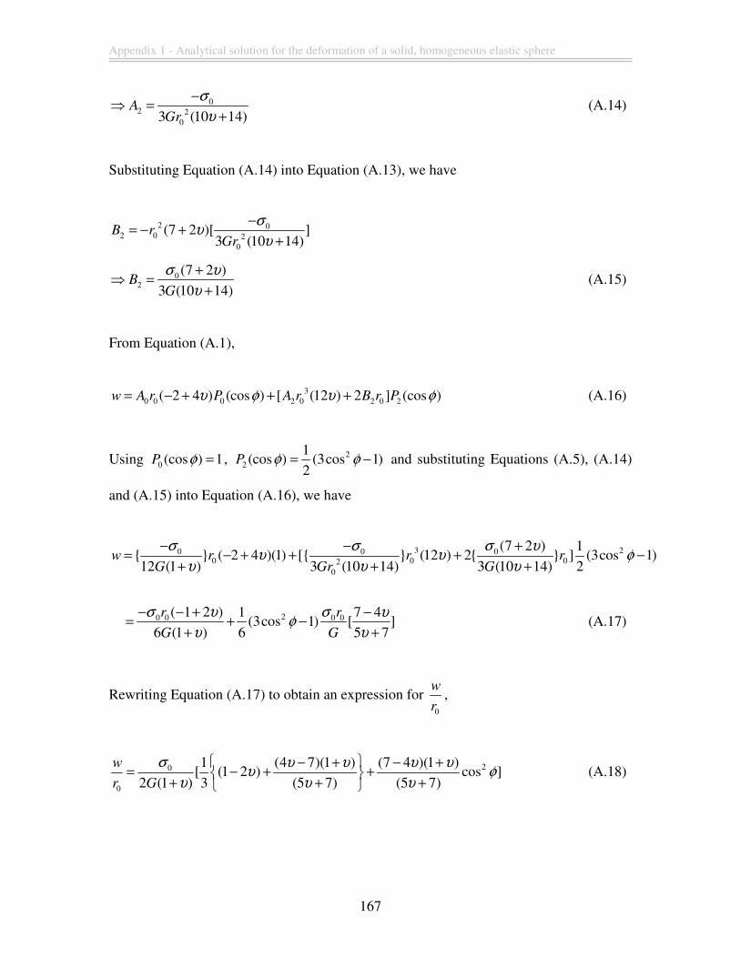
Appendix 1 - Analytical solution for the deformation of a solid, homogeneous elastic sphere
167
02 2
03 (10 14)A
Gr
σ
υ
−⇒ =
+ (A.14)
Substituting Equation (A.14) into Equation (A.13), we have
2 02 0 2
0
(7 2 )[ ]3 (10 14)
B rGr
συ
υ
−= − +
+
02
(7 2 )
3 (10 14)B
G
σ υ
υ
+⇒ =
+ (A.15)
From Equation (A.1),
30 0 0 2 0 2 0 2( 2 4 ) (cos ) [ (12 ) 2 ] (cos )w A r P A r B r Pυ φ υ φ= − + + + (A.16)
Using 0 (cos ) 1P φ = , 22
1(cos ) (3cos 1)
2P φ φ= − and substituting Equations (A.5), (A.14)
and (A.15) into Equation (A.16), we have
3 20 0 00 0 02
0
(7 2 ) 1{ } ( 2 4 )(1) [{ } (12 ) 2{ } ] (3cos 1)12 (1 ) 3 (10 14) 3 (10 14) 2
w r r rG Gr G
σ σ σ υυ υ φ
υ υ υ
− − += − + + + −
+ + +
20 0 0 0( 1 2 ) 1 7 4(3cos 1) [ ]
6 (1 ) 6 5 7
r r
G G
σ υ σ υφ
υ υ
− − + −= + −
+ + (A.17)
Rewriting Equation (A.17) to obtain an expression for 0
w
r,
20
0
1 (4 7)(1 ) (7 4 )(1 )[ (1 2 ) cos ]
2 (1 ) 3 (5 7) (5 7)
w
r G
σ υ υ υ υυ φ
υ υ υ
− + − += − + +
+ + + (A.18)
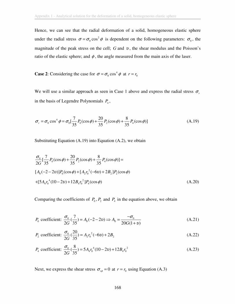
Appendix 1 - Analytical solution for the deformation of a solid, homogeneous elastic sphere
168
Hence, we can see that the radial deformation of a solid, homogeneous elastic sphere
under the radial stress 20 cosσ σ φ= is dependent on the following parameters: 0σ , the
magnitude of the peak stress on the cell; G and υ , the shear modulus and the Poisson’s
ratio of the elastic sphere; and φ , the angle measured from the main axis of the laser.
Case 2: Considering the case for 40 cosσ σ φ= at 0r r=
We will use a similar approach as seen in Case 1 above and express the radial stress r
σ
in the basis of Legendre Polynomials n
P ,
40 0 0 2 4
7 20 8cos [ (cos ) (cos ) (cos )]
35 35 35rP P Pσ σ φ σ φ φ φ= = + + (A.19)
Substituting Equation (A.19) into Equation (A.2), we obtain
00 2 4
7 20 8[ (cos ) (cos ) (cos )]
2 35 35 35P P P
G
σφ φ φ+ + =
20 0 2 0 2 2[ ( 2 2 )] (cos ) [ ( 6 ) 2 ] (cos )A P A r B Pυ φ υ φ− − + − +
4 24 0 4 0 4[5 (10 2 ) 12 ] (cos )A r B r Pυ φ+ − + (A.20)
Comparing the coefficients of 0P , 2P and 4P in the equation above, we obtain
0P coefficient: 0 00 0
7( ) ( 2 2 )
2 35 20 (1 )A A
G G
σ συ
υ
−= − − ⇒ =
+ (A.21)
2P coefficient: 202 0 2
20( ) ( 6 ) 2
2 35A r B
G
συ= − + (A.22)
4P coefficient: 4 204 0 4 0
8( ) 5 (10 2 ) 12
2 35A r B r
G
συ= − + (A.23)
Next, we express the shear stress 0rφσ = at 0r r= using Equation (A.3)
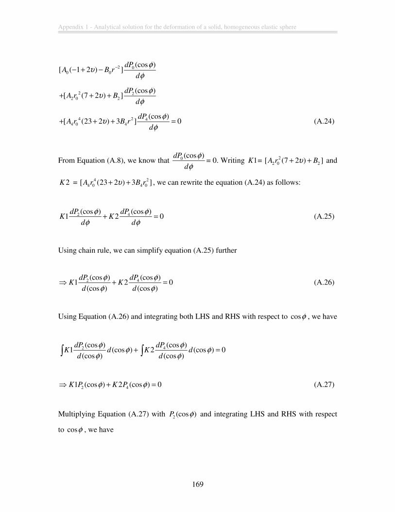
Appendix 1 - Analytical solution for the deformation of a solid, homogeneous elastic sphere
169
2 00 0
(cos )[ ( 1 2 ) ]
dPA B r
d
φυ
φ−− + −
2 22 0 2
(cos )[ (7 2 ) ]
dPA r B
d
φυ
φ+ + +
4 2 44 0 4
(cos )[ (23 2 ) 3 ] 0
dPA r B r
d
φυ
φ+ + + = (A.24)
From Equation (A.8), we know that 0 (cos )dP
d
φ
φ= 0. Writing 1K = 2
2 0 2[ (7 2 ) ]A r Bυ+ + and
2K = 4 24 0 4 0[ (23 2 ) 3 ]A r B rυ+ + , we can rewrite the equation (A.24) as follows:
2 4(cos ) (cos )1 2 0
dP dPK K
d d
φ φ
φ φ+ = (A.25)
Using chain rule, we can simplify equation (A.25) further
2 4(cos ) (cos )1 2 0
(cos ) (cos )
dP dPK K
d d
φ φ
φ φ⇒ + = (A.26)
Using Equation (A.26) and integrating both LHS and RHS with respect to cosφ , we have
2 4(cos ) (cos )1 (cos ) 2 (cos ) 0
(cos ) (cos )
dP dPK d K d
d d
φ φφ φ
φ φ+ =∫ ∫
2 41 (cos ) 2 (cos ) 0K P K Pφ φ⇒ + = (A.27)
Multiplying Equation (A.27) with 2 (cos )P φ and integrating LHS and RHS with respect
to cosφ , we have
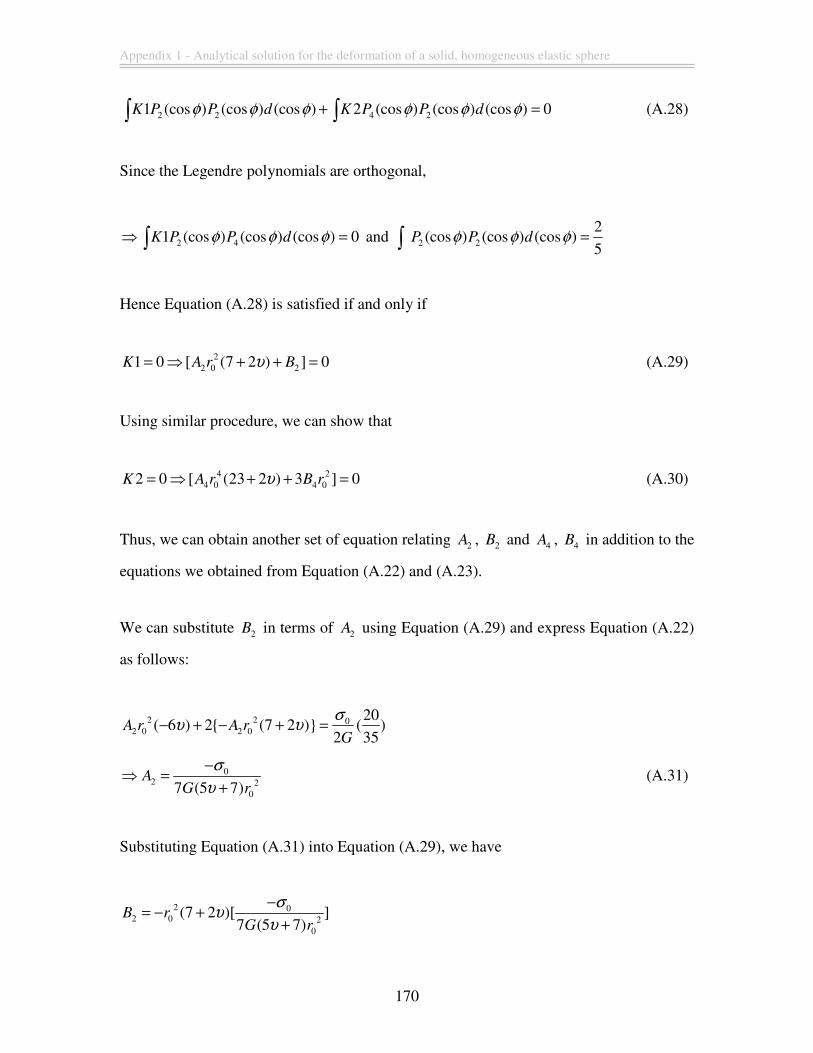
Appendix 1 - Analytical solution for the deformation of a solid, homogeneous elastic sphere
170
2 2 4 21 (cos ) (cos ) (cos ) 2 (cos ) (cos ) (cos ) 0K P P d K P P dφ φ φ φ φ φ+ =∫ ∫ (A.28)
Since the Legendre polynomials are orthogonal,
2 41 (cos ) (cos ) (cos ) 0K P P dφ φ φ⇒ =∫ and 2 2
2(cos ) (cos ) (cos )
5P P dφ φ φ =∫
Hence Equation (A.28) is satisfied if and only if
22 0 21 0 [ (7 2 ) ] 0K A r Bυ= ⇒ + + = (A.29)
Using similar procedure, we can show that
4 24 0 4 02 0 [ (23 2 ) 3 ] 0K A r B rυ= ⇒ + + = (A.30)
Thus, we can obtain another set of equation relating 2A , 2B and 4A , 4B in addition to the
equations we obtained from Equation (A.22) and (A.23).
We can substitute 2B in terms of 2A using Equation (A.29) and express Equation (A.22)
as follows:
2 2 02 0 2 0
20( 6 ) 2{ (7 2 )} ( )
2 35A r A r
G
συ υ− + − + =
02 2
07 (5 7)A
G r
σ
υ
−⇒ =
+ (A.31)
Substituting Equation (A.31) into Equation (A.29), we have
2 02 0 2
0
(7 2 )[ ]7 (5 7)
B rG r
συ
υ
−= − +
+
Appendix 1 - Analytical solution for the deformation of a solid, homogeneous elastic sphere
171
02
(7 2 )
7 (5 7)B
G
σ υ
υ
+⇒ =
+ (A.32)
We can also substitute 4B in terms of 4A using Equation (A.30) to obtain the following:
2 44 0 4 03 (23 2 )B r A r υ= − +
24 4 0
1(23 2 )
3B A r υ⇒ = − + (A.33)
Substituting Equation (A.33) into Equation (A.23), we have
4 2 2 04 0 4 0 0
1 85 (10 2 ) 12[ (23 2 )] ( )
3 2 35A r A r r
G
συ υ− + − + =
04 4
0
2
105 (7 3 )A
Gr
σ
υ
−⇒ =
+ (A.34)
Substituting Equation (A.34) into Equation (A.33), we have
204 04
0
21[ ] (23 2 )
3 105 (7 3 )B r
Gr
συ
υ
−= − +
+
04 2
0
2 (23 2 )
315 (7 3 )B
Gr
σ υ
υ
+⇒ =
+ (A.35)
From Equation (A.1),
30 0 0 2 0 2 0 2( 2 4 ) (cos ) [ (12 ) 2 ] (cos )w A r P A r B r Pυ φ υ φ= − + + +
5 34 0 4 0 4[5 (2 4 ) 4 ] (cos )A r B r Pυ φ+ + + (A.36)
Using 0 (cos ) 1P φ = , 22
1(cos ) (3cos 1)
2P φ φ= − , 4 2
4
1(cos ) (35cos 30cos 3)
8P φ φ φ= − +
and substituting Equations (A.21), (A.31), (A.32), (A.34) and (A.35) into Equation
Appendix 1 - Analytical solution for the deformation of a solid, homogeneous elastic sphere
172
(A.36), we can then obtain the analytical solution for the radial deformation of a solid,
homogeneous elastic sphere under the radial stress 40 cosσ σ φ= .
Case 3: Considering the case for 60 cosσ σ φ= at 0r r=
We have carried out the analysis for the case of 60 cosσ σ φ= at 0r r= , and the results
are given below with the derivation omitted for clarity.
30 0 0 2 0 2 0 2( 2 4 ) (cos ) [ (12 ) 2 ] (cos )w A r P A r B r Pυ φ υ φ= − + + +
5 3 7 54 0 4 0 4 6 0 6 0 6[5 (2 4 ) 4 ] (cos ) [7 (4 4 ) 6 ] (cos )A r B r P A r v B r Pυ φ φ+ + + + + + (A.37)
with
00
33,
462 (1 )A
G
σ
υ
−=
+
02 2
0
55,
231 (5 7)A
G r
σ
υ
−=
+
02
55(7 2 ),
231 (5 7)B
G
υ σ
υ
+=
+
04 4
0
12,
231 (7 3 )A
G r
σ
υ
−=
+
04 2
0
4(23 2 ),
231 (7 3 )B
G r
υ σ
υ
+=
+
06 6
0
8,
231 (43 13 )A
G r
σ
υ
−=
+
04 4
0
8(47 2 ).
1155 (43 13 )B
G r
υ σ
υ
+=
+
Analytical expressions for larger values of n can also be obtained by a similar process,
although the algebra becomes increasingly complicated.


![Finite element analysis of viscoelastic nanofluid flow ...usir.salford.ac.uk/39095/1/INT J APPL COM MATH finite element viscoelastic nanofluid...element methods. Khomami et al. [54]](https://static.fdocuments.net/doc/165x107/5e7ddb53137a81676f69cb9b/finite-element-analysis-of-viscoelastic-nanofluid-flow-usir-j-appl-com-math.jpg)
