Virtual-Reality Based Interactive Exploration of ...

Virtual-Reality Based InteractiveExploration of Multiresolution Data

Oliver Kreylos1, E. Wes Bethel2, Terry J. Ligocki3, and Bernd Hamann1

1 Center for Image Processing and Integrated Computing (CIPIC), Departmentof Computer Science, University of California, Davis, One Shields Avenue,Davis, CA 95616–8562, USA

2 Applied Numerical Algorithms Group, National Energy Research and ScientificComputing Center (NERSC), Ernest Orlando Lawrence Berkeley NationalLaboratory, One Cyclotron Road, Berkeley, CA 94720, USA

3 Visualization Group, National Energy Research and Scientific ComputingCenter (NERSC), Ernest Orlando Lawrence Berkeley National Laboratory, OneCyclotron Road, Berkeley, CA 94720, USA

Summary. We describe a system supporting the interactive exploration of three-dimensional scientific data sets in a virtual reality (VR) environment. This systemaids a scientist in understanding a data set by interactively placing and manipu-lating visualization primitives, e. g., isosurfaces or streamlines, and thereby findingfeatures in the data and understanding its overall structure.

We discuss how the requirement of interactivity influences the architecture ofthe visualization system, and how to adapt standard visualization techniques towork under real-time interaction constraints.

Though we have implemented our visualization system to work with multipletypes of data sets structures – cartesian, tetrahedral, curvilinear-hexahedral andadaptive mesh refinement (AMR) – we will focus on AMR grids and show howtheir inherent multiresolution structure is useful for interactive visualization.

1 Introduction

Contemporary scientific research is performed by gathering and analyzingvast amounts of data. Regardless of whether this data is the result of real-world measurements or numerical simulations, extracting information fromdata becomes more and more difficult as the amount of data grows. Scientificvisualization is becoming a major tool for research: The human visual systemis unparalleled in its capacity to see patterns or detect features in data.

We concentrate on scalar- or vector-valued trivariate functions, i. e., func-tions of the type fs:Ω → R or fv:Ω → R3, where Ω ⊂ R3 is some three-dimensional domain. We will also consider time-varying data sets, where thefunctions’ domains are Ω × [a, b], where [a, b] ⊂ R is some interval of time.

1.1 Visual Exploration

Typically, visualization is used for two different purposes: First, it can beused to gain understanding of phenomena underlying data; second, it can be

2 Oliver Kreylos et al.

used to communicate this understanding to an audience. We concentrate onthe first purpose, visual exploration. A scientist is typically confronted witha data set from an experiment or a simulation, and the task is to gain insightinto the data. Often, especially when data is generated by a simulation, it isalso necessary to show that the simulation system generated meaningful dataat all; in this context, visual exploration becomes a debugging tool.

Visual exploration is most useful when applied early during data genera-tion. Simulations generating large data sets typically run for long periods oftime, even when using a supercomputer. If a visual exploration system canbe used to visualize preliminary or evolving simulation results, it might bepossible to detect errors in the simulation early, and to fix them by changingsimulation parameters “on the fly.” This interplay between visualization andsimulation, also referred to as computational steering, can be very helpful inincreasing the performance of a simulation system and its value for the over-all scientific investigation process. To allow coupling visualization and sim-ulation, the visualization system should be able to read the data generatedby the simulation with as little pre-processing as possible. Since simulationsystems create data in a variety of different formats (tetrahedral, cartesian,(curvilinear) hexahedral, AMR, etc.), the visualization system must supportall these data structures directly, without having to resort to converting themto a standard format by re-sampling.

When working directly on the native data structure used by a simula-tion system, the debugging power of the visual exploration system is greatlyincreased. For example, an AMR simulation program creates the grid hier-archy without intervention [1], by considering certain properties of the dataitself. If the visualization system can display the AMR data directly, it canalso display the grid structure, providing the scientist with clues about thesimulation process. We explain how to isolate the data set structure from therest of the visualization program in Sec. 3.

1.2 Benefits of VR Methods

A standard visualization system that addresses both uses of visualization(exploration and communication) usually sacrifices interactivity for imagequality. This fact can reduce the usefulness of a general-purpose system forvisual exploration. For example, a data set might be the result of a numericalsimulation of air flow around an aircraft wing, and the task is to determinewhether the design fulfills the required aerodynamic objectives and how thewing design could be improved. In a standard visualization system, this taskmight be handled in the following way:

1. Place some visualization primitives, e. g., streamlines, at points consid-ered “interesting.”

2. Generate an image or multiple images.3. If the imagery does not reveal anything exciting, repeat from step 1.

Interactive Data Exploration 3

There are several problems with such an approach. First, a user has tospecify at which points to place primitives. Specifying positions in 3D spaceusing a 2D input device, e. g., a mouse, is awkward. Second, the process ofimage generation is time-consuming, and with placement of primitives essen-tially being a trial-and-error process, the overall time spent on analysis cangrow prohibitively large. Even worse, merely seconds of delay between placinga primitive and seeing a resulting image can make intuitive exploration of adata set almost impossible. Third, even when an image reveals some features,it is only a 2D projection of a 3D data set and can be misleading concerningspatial relationships of features.

(a) (b)

Fig. 1. Exploration of vector field on tetrahedral mesh with embedded geometry.(a) Visualization with streamlines (b) Visualization with streamribbons

VR can attack all three of these problems, making the exploration processmuch more productive. There are probably more contradicting definitions ofVR in existence than there are VR researchers; but for the purposes of thispaper, a system is considered a VR system if it offers at least the followingfunctionalities:

• True 3D (stereoscopic) display with head tracking, i. e., support of a dis-play that is dependent on a user’s true eye position in space, updated atleast at 30 Hz to create the illusion that the visualization is “real,”

• support of six-degree-of-freedom (6-DOF) input devices to allow a userto directly interact with and manipulate the visualization, and

• interactivity, meaning that the system’s response time to user actions issmall enough to seem immediate (within 0.05 s to 0.1 s).

With a VR system like this, the basic exploration loop remains the same;but with immediate response, a user is able to move a visualization primitivedirectly through a 3D data set until something interesting is visualized. Theimmediate update of displayed imagery, leading to an animation of a visu-alization primitive’s behaviour, provides valuable clues as to where to movethe primitive next in order to “close in” on a feature.


1.3 Real-time Constraints

The goal of implementing an interactive, real-time visualization system im-poses several constraints on the visualization methods that can be supported.A severly limiting constraint is the display constraint, which requires that allimagery can be rendered at a frame rate of at least 30 Hz per eye. If the framerate drops below 30 Hz, the display will appear “choppy,” which can lead toeye strain and even motion sickness. Since users cannot hold their heads per-fectly still, displayed stereo images have to be updated continuously, evenif the visualization itself does not change. This forbids using very costly vi-sualization methods, e. g., high-quality volume rendering [7]. Visualizationmethods of choice are the ones based on graphics primitives supported byavailable graphics hardware, e. g., isosurfaces, streamlines or streamribbons.

Even when considering only visualization methods supported by availablegraphics hardware, generating the visualizations can still be time-consuming.Though it is not necessary to update the visualization for every frame, shouldupdating require more than 0.1 s, the system is “lagging,” defeating the goalof interactivity. We refer to this constraint as the update constraint. Thisimplies, for example, that a standard implementation of the Marching-Cubes(MC) isosurfacing algorithm [8–10] is not appropriate for visual exploration:Though the resulting isosurface triangulation might consist of a relativelysmall number of triangles, small enough to satisfy the display constraint, thetime to generate the triangles might require seconds or minutes for large datasets, violating the update constraint. In Sec. 3.2, we explain how to adaptstandard visualization methods to an interactive environment.

1.4 Related Work

Data visualization based on VR is not new. Several early important contri-butions were made by NASA scientists: The NASA Virtual Wind Tunnel,described, for example, by Bryson and Levit [5], is a visualization system fortime-varying vector-valued data. Meyer and Globus [6] describe an interactiveisosurface generator for scalar-valued data.

2 User Interface

User interfaces for virtual-reality environments are still an area of activeresearch, and an interface paradigm agreed upon by most researchers hasstill to be developed. For our system, we implemented the simple gesture-and menu-driven user interface described in the following sections.

2.1 Available VR Devices

The design of the user interface is dependent on the underlying VR hard-ware, especially on the number of input devices and their degrees of freedom,


and the number and arrangement of buttons available. We implemented oursystem for two classes of VR hardware:

Virtual Workbench A virtual workbench is a semi-immersive VR systemconsisting of a large display screen, a pair of head-tracked shutter glasses,and three 6-DOF input devices: One stylus with a single button, and twopinch gloves with four buttons each, that can be activated by pinchingthe thumb and one of the other fingers.

CAVE A CAVE is a semi-immersive VR system consisting of one or morelarge display screens, a pair of head-tracked shutter glasses, and a single6-DOF input device: A wand with three buttons and a pressure-sensitivejoystick on it. CAVE systems come in different configurations, from asingle-screen desk-like environment (ImmersaDesk) to a ten-by-ten-by-ten foot cube with five display screens as walls (“classic” CAVE). For thepurposes of our system, we can treat all these identically, because theyprovide the same functionality in input devices, and the differences of thedisplay hardware are hidden by a common application program interface,the CAVE library.

2.2 VR Toolkit

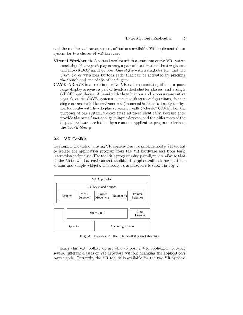
To simplify the task of writing VR applications, we implemented a VR toolkitto isolate the application program from the VR hardware and from basicinteraction techniques. The toolkit’s programming paradigm is similar to thatof the Motif window environment toolkit: It supplies callback mechanisms,actions and simple widgets. The toolkit’s architecture is shown in Fig. 2.

InputDevices

VR Application

DisplayMenu

SelectionPointer

Movement NavigationPointer

Selection

Callbacks and Actions

VR Toolkit

Operating SystemOpenGL

Fig. 2. Overview of the VR toolkit’s architecture

Using this VR toolkit, we are able to port a VR application betweenseveral different classes of VR hardware without changing the application’ssource code. Currently, the VR toolkit is available for the two VR systems


listed above, and a version for desktop workstations is used for applicationtesting purposes.

2.3 3D Pointer

The main selection and interaction is done with the 3D pointer. This equiv-alent to a single-button mouse in a 2D window system is used to inquiredata values at any point inside a data set, to place and drag new primitives,and to select existing ones. In the Virtual Workbench environment, we usethe stylus as 3D mouse; in the CAVE environment, we use the wand and itsleftmost button, the mouse button.

2.4 Navigation

In order to explore large data sets, a user must be able to freely navigatethrough the data sets. It must be possible to get an overview of the wholedata set, and it must also be possible to zoom in to a small region of space.Furthermore, navigation must be as intuitive as possible to not interfere withthe exploration process. We chose to implement navigation by direct ma-nipulation: Instead of using indirect navigation tools, e. g., scrollbars in 2Dwindow systems, a user can directly “grab” a point in space using a 6-DOFinput device. Grabbing will fix the data set’s coordinate system with respectto the input device’s coordinate system, and any movement (translation orrotation) of the input device while a point is grabbed will move the wholedata set accordingly, allowing panning and rotating.

In the Virtual Workbench environment, we employ pinch gloves for nav-igation. A point can be grabbed with either hand, by pinching thumb andindex finger. This two-handed navigation suits both left- and right-handedusers, and it also allows to navigate with one hand even while the other handis interacting with the data set using the stylus. In the CAVE environment,the wand is switched into navigation mode using its middle button, the nav-igation button.

Though it is possible to grab any point in space, inexperienced users willintuitively only grab parts of displayed geometry, either existing visualizationprimitives or models embedded in the data set. Experiments have shownthat this is not a serious limitiation; users get adjusted to the navigationparadigm quickly (in a matter of minutes) and are able to pan/rotate datasets according to their wishes.

While navigation involving panning and rotating is very intuitive, zoomingis more difficult to implement. This is probably due to the fact that zoomingis not possible in the real world: While every child learns how to pick up anobject and move it around to inspect it from all sides from a very early ageon, there is no natural way to enlarge an object. We implemented zooming indifferent ways, depending on the available input devices. In an environmentwith two input devices, a user can grab one point in space with each device.


Then, pulling the two devices apart will zoom in, and pushing them togetherwill zoom out. We decided to make the zoom factor proportional to the twodevice’s distance1; following this principle, the apparent motion of the dataset will relate to the input devices’ motion in a natural way. In a single inputdevice environment, we reserved a special button combination on the inputdevice for switching into zoom mode. A user can zoom in by pulling the inputdevice towards her, and zoom out by pushing the input device away.

In the Virtual Workbench environment, both pinch gloves are used forzooming. First, the user will grab one point with one glove, enabling panningand rotating. Then the user will grab another point with the second glove,enabling zooming. The data set’s coordinate system is still fixed to the firstglove while zooming; this enables panning, rotating and zooming simulta-neously. In the CAVE environment, zooming is activated while the wand isalready in navigation mode. Pressing the mouse button while the navigationbutton is held stops panning and rotating and enables zooming. Luckily, thetwo buttons are close enough to allow even inexperienced users to press bothat the same time using one thumb. Still, the restriction to only one inputdevice limits the usability of the system. Experiments have shown that theambidexterous Virtual Workbench is more intuitive and makes it easier tonavigate to a desired viewpoint.

Even in an environment with two devices, experiments show that inex-perienced users will hardly use the zoom feature. Instead, they tend to pulla part of the data set they want to examine closer to their eyes, making itappear larger. This is a natural reaction, but it clashes with the limitations ofthe graphics system. Due to the stereo rendering, objects close to the user’seyes will be out of focus, and due to inaccuracies of head tracking, objectswill not appear to be stable but move erratically. Correctly using the zoomfeature to inspect an area more closely requires some training.

2.5 Higher-level Functions

To access higher-level program functions, e. g., selecting tools or changingvisualization parameters, we provide a simple system of cascading popupmenus. The main menu can be popped up at any position and orientation inspace. While it is displayed, the 3D pointer is used to select menu entries orpop up submenus.

In the Virtual Workbench environment, the main menu is popped up bypinching thumb and middle finger of one hand. While the menu is displayed,it will move with the hand, allowing the user to move it to a position whereit is convenient to select entries using the stylus and the other hand. In theCAVE environment, the rightmost wand button, the menu button, will popup the main menu at the current wand position. As soon as the menu is

1 z = ‖p1 − p2‖/d0, where pi are the device’s positions, and d0 is their initialdistance at the time grabbing occured.


displayed, the wand is used to activate entries or popup submenus. Releasingthe menu button selects the currently active menu item.

3 System Architecture

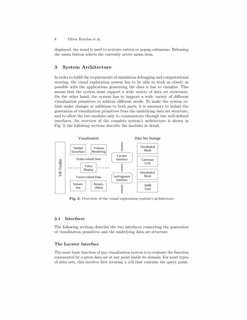
In order to fulfill the requirements of simulation debugging and computationalsteering, the visual exploration system has to be able to work as closely aspossible with the applications generating the data it has to visualize. Thismeans that the system must support a wide variety of data set structures.On the other hand, the system has to support a wide variety of differentvisualization primitives to address different needs. To make the system ro-bust under changes or additions to both parts, it is necessary to isolate thegeneration of visualization primitives from the underlying data set structure,and to allow the two modules only to communicate through two well-definedinterfaces. An overview of the complete system’s architecture is shown inFig. 3; the following sections describe the modules in detail.

SeededIsosurface

ValueDisplay

VolumeRendering

Stream-line

Stream-ribbon

LocatorInterface

IsoFragmentInterface

TetrahedralMesh

CartesianGrid

HexahedralMesh

AMRGrid

Visualization Data Set Storage

Scalar-valued Data

Vector-valued DataVR

Too

lkit

Fig. 3. Overview of the visual exploration system’s architecture

3.1 Interfaces

The following sections describe the two interfaces connecting the generationof visualization primitives and the underlying data set structure.

The Locator Interface

The most basic function of any visualization system is to evaluate the functionrepresented by a given data set at any point inside its domain. For most typesof data sets, this involves first locating a cell that contains the query point,


and then applying some interpolation scheme to calculate the value at thequery point’s position. To allow maximal efficiency, we defined the Locatorinterface to contain both functions separately:

• bool locatePoint(p, bool traceHint) prepares a locator to interpo-late the data set’s value at position p. The function’s return value indi-cates whether the given point p is inside the data set’s domain. If thereturn value is false, it is not possible to determine the data set’s value.For some data set structures, locating a point “from scratch” might bevery expensive; it might become much less difficult when a locator canuse the fact that the new point it has to locate is close to the last locatedpoint. The parameter traceHint is a hint, provided by the visualizationsystem, that the given point is close to the last point, and that using thisinformation might be beneficial. Several typical visualization primitives,e. g., streamlines, evaluate a data set at a long sequence of points beingvery close to each other. In some cases, using the traceHint parameterresulted in speed-ups of an order of magnitude.

• ValueType interpolateValue(void) calculates the data set’s value atthe last located position.

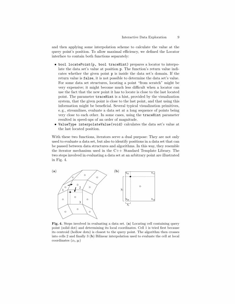
With these two functions, iterators serve a dual purpose: They are not onlyused to evaluate a data set, but also to identify positions in a data set that canbe passed between data structures and algorithms. In this way, they resemblethe iterator mechanism used in the C++ Standard Template Library. Thetwo steps involved in evaluating a data set at an arbitrary point are illustratedin Fig. 4.

(a)

12

3

(b)

xl

yl

v00 v10

v01 v11

Fig. 4. Steps involved in evaluating a data set. (a) Locating cell containing querypoint (solid dot) and determining its local coordinates. Cell 1 is tried first becauseits centroid (hollow dots) is closest to the query point. The algorithm then crossesinto cells 2 and finally 3 (b) Bilinear interpolation used to evaluate the cell at localcoordinates (xl, yl)


The IsoFragment Interface

The IsoFragment interface has a more specific purpose than the Locatorinterface: It is used to generate seeded isosurfaces, as will be explained inSec. 3.2. An IsoFragment identifies a cell in a data set, and it provides thefollowing two functions:

• setCell(Locator loc) associates an IsoFragment with the data set cellcontaining the point most recently located by the Locator. This functionis used to seed an isosurface.

• expandSurface(ValueType isovalue, Queue expandNext) creates thefragment of the surface connecting all points with value isovalue insidethe associated cell, and puts all the cell’s neighbours sharing faces thatare intersected by the isosurface in the expansion queue.

3.2 Supported Visualization Primitives

The choices of visualization primitives for visual exploration systems are lim-ited by the two constraints discussed in Sec. 1.3: The graphics system mustbe able to display all active primitives at a framerate of at least 30 Hz pereye (display constraint), and the visualization system must be able to updateall primitives the user is interacting with at a rate of at least 10 Hz (updateconstraint). Some common primitives, e. g., streamlines, are almost directlyapplicable to visual exploration, whereas others, e. g., isosurfaces, have to beadapted to be usable.

Data Value Display

The most basic tool, hardly a visualization primitive, is to display the datavalue at the current 3D pointer location. It can be applied to both scalar-and vector-valued data sets. The only operation required by this tool is cal-culation of a function value for an arbitrary point, given in the data set’scoordinate system. This operation is directly supported by the Locator in-terface described in Sec. 3.1. Since the 3D pointer is traced by the systemat a rate of 30Hz, it usually only moves a short distance between two pointlocation requests. Communicating this fact to the Locator interface using thetraceHint parameter mentioned in Sec. 3.1 can increase system performance,depending on the underlying data set structure.

Primitives for Scalar-valued Data Sets

The following primitives apply only to scalar-valued data sets, i. e., thosedefining functions f :Ω → R.


Seeded Isosurfaces The most often used visualization primitive for scalar-valued data is the isosurface, connecting all points in space having identicalfunction value [8]: For a scalar-valued function f :Ω ⊂ R3 → R, the iso-surface I(v) for isovalue v is defined by I(v) =

x ∈ Ω

∣∣ f(x) = v. In

standard systems, isosurfaces are typically generated using some variationof the Marching-Cubes algorithm [9]. In this algorithm, isosurface fragmentsare generated independently for each cell of the data set. This algorithm hasa runtime proportional to the number of cells, and generally runs severalseconds to minutes for large data sets.

To use isosurfaces in an interactive visualization system, we have to changetheir generation to satisfy both display and update constraint, see Sec. 1.3.The basic idea is to generate isosurfaces incrementally starting from a givenpoint in space, instead of globally starting from a given function value. In oursystem, a user can move the 3D pointer to an arbitrary position in space andseed an isosurface there. A seeded isosurface is generated using the followingmain steps:

1. Determine the cell containing the 3D pointer and calculate the functionvalue at the pointer’s position. Store the found value as the isovalue touse, and put the found cell in the expansion queue.

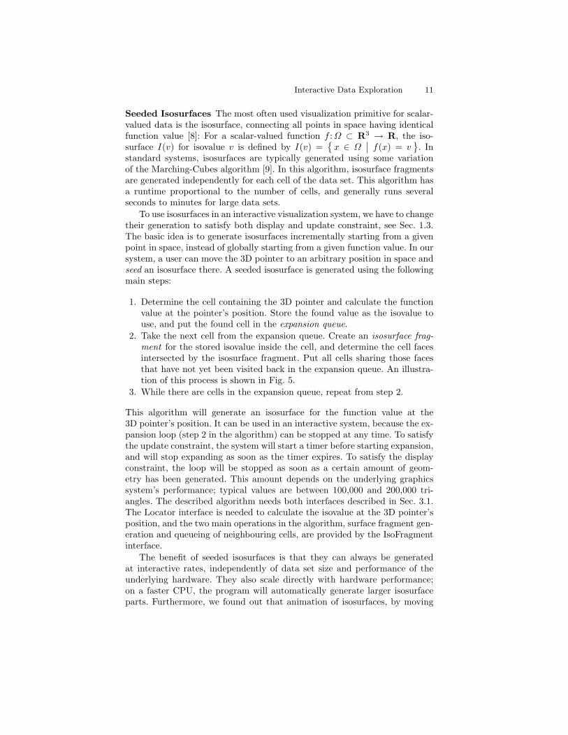
2. Take the next cell from the expansion queue. Create an isosurface frag-ment for the stored isovalue inside the cell, and determine the cell facesintersected by the isosurface fragment. Put all cells sharing those facesthat have not yet been visited back in the expansion queue. An illustra-tion of this process is shown in Fig. 5.

3. While there are cells in the expansion queue, repeat from step 2.

This algorithm will generate an isosurface for the function value at the3D pointer’s position. It can be used in an interactive system, because the ex-pansion loop (step 2 in the algorithm) can be stopped at any time. To satisfythe update constraint, the system will start a timer before starting expansion,and will stop expanding as soon as the timer expires. To satisfy the displayconstraint, the loop will be stopped as soon as a certain amount of geom-etry has been generated. This amount depends on the underlying graphicssystem’s performance; typical values are between 100,000 and 200,000 tri-angles. The described algorithm needs both interfaces described in Sec. 3.1.The Locator interface is needed to calculate the isovalue at the 3D pointer’sposition, and the two main operations in the algorithm, surface fragment gen-eration and queueing of neighbouring cells, are provided by the IsoFragmentinterface.

The benefit of seeded isosurfaces is that they can always be generatedat interactive rates, independently of data set size and performance of theunderlying hardware. They also scale directly with hardware performance;on a faster CPU, the program will automatically generate larger isosurfaceparts. Furthermore, we found out that animation of isosurfaces, by moving


Fig. 5. Expanding a seeded isosurface. TheIsoFragment interface generates a fragment ofan isosurface inside a cell, and puts all neigh-bouring cells the isosurface continues into in anexpansion queue

the 3D pointer while continuosly seeding, enables a user to quickly gain un-derstanding of the behaviour of the data set in a region of space.

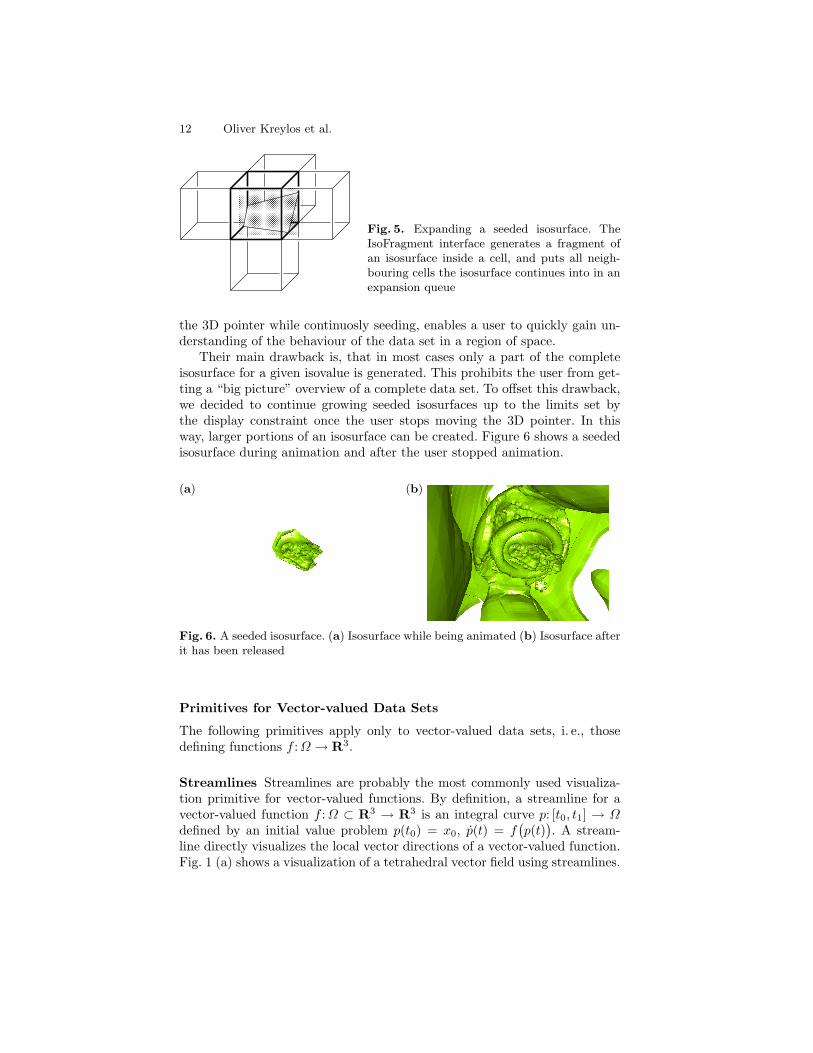
Their main drawback is, that in most cases only a part of the completeisosurface for a given isovalue is generated. This prohibits the user from get-ting a “big picture” overview of a complete data set. To offset this drawback,we decided to continue growing seeded isosurfaces up to the limits set bythe display constraint once the user stops moving the 3D pointer. In thisway, larger portions of an isosurface can be created. Figure 6 shows a seededisosurface during animation and after the user stopped animation.

(a) (b)

Fig. 6. A seeded isosurface. (a) Isosurface while being animated (b) Isosurface afterit has been released

Primitives for Vector-valued Data Sets

The following primitives apply only to vector-valued data sets, i. e., thosedefining functions f :Ω → R3.

Streamlines Streamlines are probably the most commonly used visualiza-tion primitive for vector-valued functions. By definition, a streamline for avector-valued function f :Ω ⊂ R3 → R3 is an integral curve p: [t0, t1] → Ωdefined by an initial value problem p(t0) = x0, p(t) = f

(p(t)

). A stream-

line directly visualizes the local vector directions of a vector-valued function.Fig. 1 (a) shows a visualization of a tetrahedral vector field using streamlines.


In our system, a user can create a streamline by selecting a startingpoint x0 ∈ Ω inside the data set’s domain. The points defining the streamlineare then generated from the initial value problem using an adaptive step-sizefourth-order Runge–Kutta method. This generation algorithm satisfies bothreal-time constraints; streamlines are generated one point at a time, and thegeneration can be interrupted when a computation timer runs out. As all in-teractive visualization primitives, the user can animate a streamline by mov-ing the 3D pointer while the streamline is continuously regenerated. We foundout that this animation is very helpful in understanding the behaviour of thefunction represented by a data set. By observing a streamline’s “reaction” tomoving the start point, a user can intuitively “home in” to critical points,and can get an understanding of the function’s vector field topology [3].

When using a Runge–Kutta method to generate streamlines, the onlyfunctionality needed is to evaluate the given data set at a sequence of positionsinside its domain. This functionality is provided by the Locator interface. Weobserve that subsequent evaluation positions in a Runge–Kutta computationare very close to each other. Thus, to maximize performance,our system usesthe traceHint parameter to the locatePoint function to communicate thisfact to the data set storage.

Streamribbons Streamlines as described above only visualize the local vec-tor directions of a vector-valued functions. Often it is desirable to also directlyvisualize derived properties of a vector-valued function. Streamribbons are ageneralization of streamlines that directly visualize the local vector directionand the local vorticity of a vector-valued function [4]. Instead of being a sin-gle curve, a streamribbon is rendered as a thin strip, whose rotation aroundits longitudinal axis is proportional to the dot product of the visualized func-tion’s local vorticity and the streamribbon’s direction. Fig. 1 (b) shows avisualization of a tetrahedral vector field using streamribbons.

Streamribbons are generated similarly to streamlines: A fourth-order Run-ge–Kutta method is used to iteratively solve the defining initial value prob-lem, and the data set’s vorticity is evaluated directly through the Locatorinterface. As for streamlines, the computation can be interrupted at any timeto satisfy the real-time constraints.

3.3 Data Set Structures

In this section, we describe the different data set structures implemented inour system, and how the two interfaces are implemented for each.

Cartesian Grids

For our purposes, cartesian grids are the simplest data set structure. A carte-sian grid consists of a three-dimensional rectangular arrangement of i× j×krectangular hexahedral cells, where each cell is of identical size sx × sy × sz.


Locating a point inside a cartesian grid merely involves multiplication andmodulo division operations, and interpolating the function value at a pointinside a cell is done using trilinear interpolation.

To generate an isosurface fragment inside a cell, we use a standard Mar-ching-Cubes case table; to enumerate all intersected neighbours of a cell, weuse the implicit neighbourhood relation imposed by the grid structure.

Tetrahedral Meshes

In tetrahedral meshes, locating a point involves finding the tetrahedron con-taining it, and calculating the point’s barycentric coordinates inside thattetrahedron. To locate a point, we use the following two-stage approach:

1. Find the tetrahedron whose centroid is closest to the point in question.We implemented this by computing all cell centroids upon loading a dataset, and storing them in an octree to later retrieve them using a closest-point query. If the traceHint parameter is set, skip this step and use thetetrahedron containing the last located point.

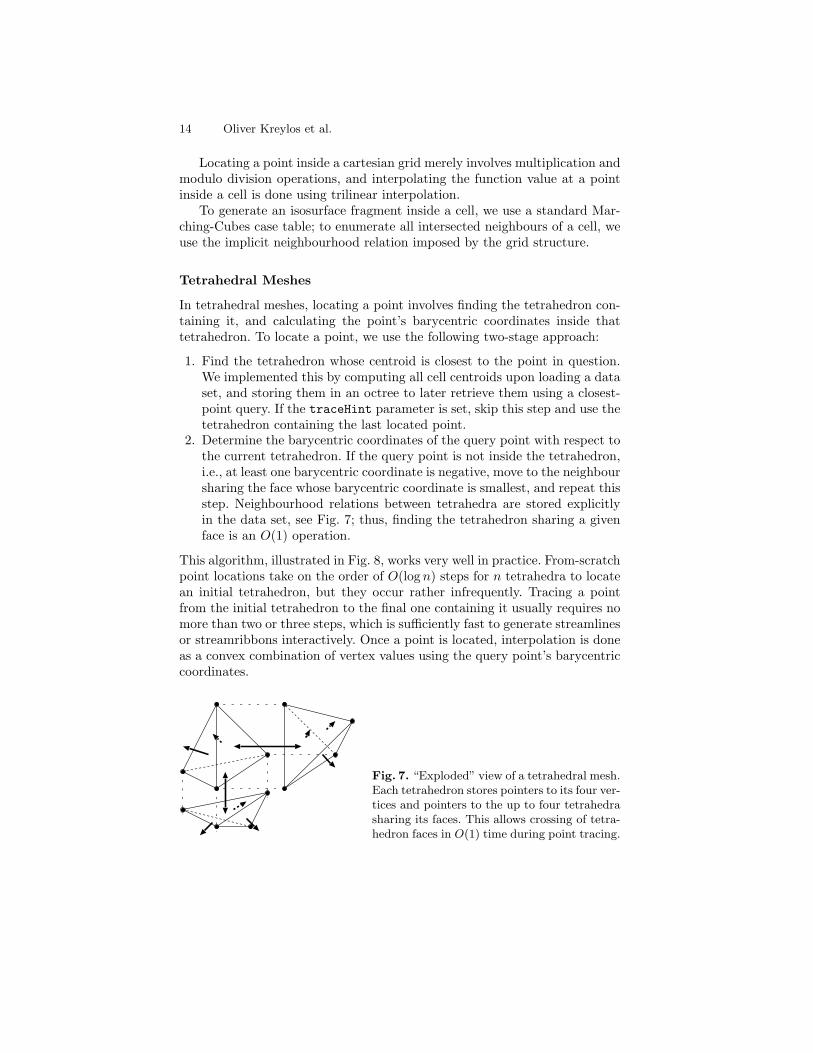
2. Determine the barycentric coordinates of the query point with respect tothe current tetrahedron. If the query point is not inside the tetrahedron,i.e., at least one barycentric coordinate is negative, move to the neighboursharing the face whose barycentric coordinate is smallest, and repeat thisstep. Neighbourhood relations between tetrahedra are stored explicitlyin the data set, see Fig. 7; thus, finding the tetrahedron sharing a givenface is an O(1) operation.

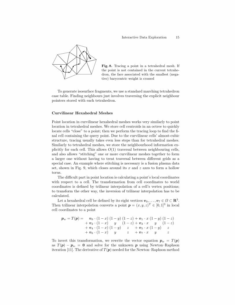
This algorithm, illustrated in Fig. 8, works very well in practice. From-scratchpoint locations take on the order of O(log n) steps for n tetrahedra to locatean initial tetrahedron, but they occur rather infrequently. Tracing a pointfrom the initial tetrahedron to the final one containing it usually requires nomore than two or three steps, which is sufficiently fast to generate streamlinesor streamribbons interactively. Once a point is located, interpolation is doneas a convex combination of vertex values using the query point’s barycentriccoordinates.

Fig. 7. “Exploded” view of a tetrahedral mesh.Each tetrahedron stores pointers to its four ver-tices and pointers to the up to four tetrahedrasharing its faces. This allows crossing of tetra-hedron faces in O(1) time during point tracing.


Fig. 8. Tracing a point in a tetrahedral mesh. Ifthe point is not contained in the current tetrahe-dron, the face associated with the smallest (nega-tive) barycentric weight is crossed

To generate isosurface fragments, we use a standard marching tetrahedroncase table. Finding neighbours just involves traversing the explicit neighbourpointers stored with each tetrahedron.

Curvilinear Hexahedral Meshes

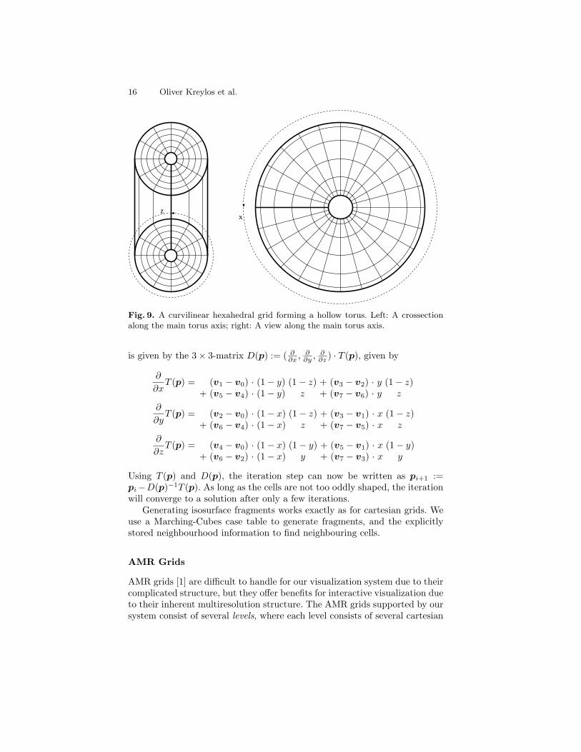
Point location in curvilinear hexahedral meshes works very similarly to pointlocation in tetrahedral meshes. We store cell centroids in an octree to quicklylocate cells “close” to a point; then we perform the tracing loop to find the fi-nal cell containing the query point. Due to the curvilinear cells’ almost-cubicstructure, tracing usually takes even less steps than for tetrahedral meshes.Similarly to tetrahedral meshes, we store the neighbourhood information ex-plicitly for each cell. This allows O(1) traversal between neighbouring cells,and also allows “stitching” one or more curvilinear meshes together to forma larger one without having to treat traversal between different grids as aspecial case. An example where stitching is necessary is a fusion plasma dataset, shown in Fig. 9, which closes around its x and z axes to form a hollowtorus.

The difficult part in point location is calculating a point’s local coordinateswith respect to a cell. The transformation from cell coordinates to worldcoordinates is defined by trilinear interpolation of a cell’s vertex positions;to transform the other way, the inversion of trilinear interpolation has to becalculated.

Let a hexahedral cell be defined by its eight vertices v0, . . . ,v7 ∈ Ω ⊂ R3.Then trilinear interpolation converts a point p = (x, y, z)T ∈ [0, 1]3 in localcell coordinates to a point

pw = T (p) = v0 · (1− x) (1− y) (1− z) + v1 · x (1− y) (1− z)+ v2 · (1− x) y (1− z) + v3 · x y (1− z)+ v4 · (1− x) (1− y) z + v5 · x (1− y) z+ v6 · (1− x) y z + v7 · x y z

To invert this transformation, we rewrite the vector equation pw = T (p)as T (p) − pw = 0 and solve for the unknown p using Newton–Raphsoniteration [11]. The derivative of T (p) needed for the Newton–Raphson method


xz

Fig. 9. A curvilinear hexahedral grid forming a hollow torus. Left: A crossectionalong the main torus axis; right: A view along the main torus axis.

is given by the 3× 3-matrix D(p) := ( ∂∂x , ∂

∂y , ∂∂z ) · T (p), given by

∂

∂xT (p) = (v1 − v0) · (1− y) (1− z) + (v3 − v2) · y (1− z)

+ (v5 − v4) · (1− y) z + (v7 − v6) · y z

∂

∂yT (p) = (v2 − v0) · (1− x) (1− z) + (v3 − v1) · x (1− z)

+ (v6 − v4) · (1− x) z + (v7 − v5) · x z

∂

∂zT (p) = (v4 − v0) · (1− x) (1− y) + (v5 − v1) · x (1− y)

+ (v6 − v2) · (1− x) y + (v7 − v3) · x y

Using T (p) and D(p), the iteration step can now be written as pi+1 :=pi−D(p)−1T (p). As long as the cells are not too oddly shaped, the iterationwill converge to a solution after only a few iterations.

Generating isosurface fragments works exactly as for cartesian grids. Weuse a Marching-Cubes case table to generate fragments, and the explicitlystored neighbourhood information to find neighbouring cells.

AMR Grids

AMR grids [1] are difficult to handle for our visualization system due to theircomplicated structure, but they offer benefits for interactive visualization dueto their inherent multiresolution structure. The AMR grids supported by oursystem consist of several levels, where each level consists of several cartesian


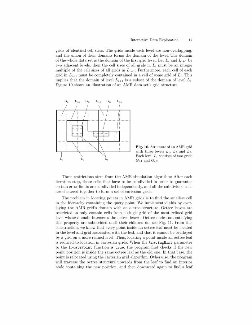
grids of identical cell sizes. The grids inside each level are non-overlapping,and the union of their domains forms the domain of the level. The domainof the whole data set is the domain of the first grid level. Let Li and Li+1 betwo adjacent levels; then the cell sizes of all grids in Li must be an integermultiple of the cell sizes of all grids in Li+1. Furthermore, each cell of eachgrid in Li+1 must be completely contained in a cell of some grid of Li. Thisimplies that the domain of level Li+1 is a subset of the domain of level Li.Figure 10 shows an illustration of an AMR data set’s grid structure.

L1 L2 L3

G1,1 G2,1 G1,2 G2,2G3,1 G3,2

Fig. 10. Structure of an AMR gridwith three levels L1, L2 and L3.Each level Li consists of two gridsGi,1 and Gi,2

These restrictions stem from the AMR simulation algorithm: After eachiteration step, those cells that have to be subdivided in order to guaranteecertain error limits are subdivided independently, and all the subdivided cellsare clustered together to form a set of cartesian grids.

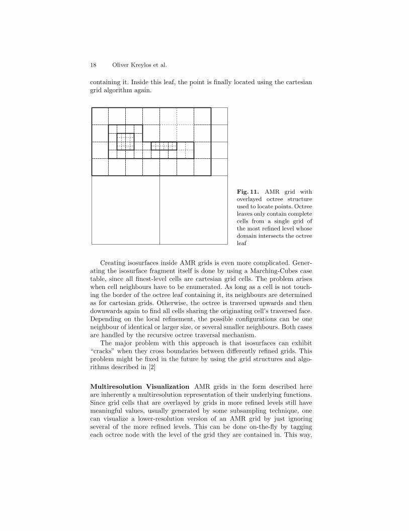
The problem in locating points in AMR grids is to find the smallest cellin the hierarchy containing the query point. We implemented this by over-laying the AMR grid’s domain with an octree structure. Octree leaves arerestricted to only contain cells from a single grid of the most refined gridlevel whose domain intersects the octree leaves. Octree nodes not satisfyingthis property are subdivided until their children do, see Fig. 11. From thisconstruction, we know that every point inside an octree leaf must be locatedin the level and grid associated with the leaf, and that it cannot be overlayedby a grid on a more refined level. Thus, locating a point inside an octree leafis reduced to location in cartesian grids. When the tracingHint parameterto the locatePoint function is true, the program first checks if the newpoint position is inside the same octree leaf as the old one. In that case, thepoint is relocated using the cartesian grid algorithm. Otherwise, the programwill traverse the octree structure upwards from the leaf to find an interiornode containing the new position, and then downward again to find a leaf


containing it. Inside this leaf, the point is finally located using the cartesiangrid algorithm again.

Fig. 11. AMR grid withoverlayed octree structureused to locate points. Octreeleaves only contain completecells from a single grid ofthe most refined level whosedomain intersects the octreeleaf

Creating isosurfaces inside AMR grids is even more complicated. Gener-ating the isosurface fragment itself is done by using a Marching-Cubes casetable, since all finest-level cells are cartesian grid cells. The problem ariseswhen cell neighbours have to be enumerated. As long as a cell is not touch-ing the border of the octree leaf containing it, its neighbours are determinedas for cartesian grids. Otherwise, the octree is traversed upwards and thendownwards again to find all cells sharing the originating cell’s traversed face.Depending on the local refinement, the possible configurations can be oneneighbour of identical or larger size, or several smaller neighbours. Both casesare handled by the recursive octree traversal mechanism.

The major problem with this approach is that isosurfaces can exhibit“cracks” when they cross boundaries between differently refined grids. Thisproblem might be fixed in the future by using the grid structures and algo-rithms described in [2]

Multiresolution Visualization AMR grids in the form described hereare inherently a multiresolution representation of their underlying functions.Since grid cells that are overlayed by grids in more refined levels still havemeaningful values, usually generated by some subsampling technique, onecan visualize a lower-resolution version of an AMR grid by just ignoringseveral of the more refined levels. This can be done on-the-fly by taggingeach octree node with the level of the grid they are contained in. This way,


interior nodes can be treated like leaves when their grid level is at least asrefined as the maximum level that should be considered at the selected level ofresolution. The other parts of the AMR grid code do not have to be changedto accomodate multiresolution visualization in this way.

4 Conclusions and Future Work

We presented an interactive VR visual exploration system that can be usedby scientists to explore large data sets of different structures. It is specificallydesigned to work closely with the simulation systems generating the visual-ized data, to allow exploration of preliminary or evolving data and to enable“computational steering.” We discussed how the requirement of interactivityhas influenced the architecture of our system and the choice of supported vi-sualization primitives and their implementation. We described how to isolatethe two major system components, visualization and data set storage, fromeach other by introducing small, well-defined interfaces, and how these inter-faces are implemented for the supported data set structures. We concentratedon visualizing AMR data, and on how to exploit the inherent multiresolutionstructure of AMR grids for interactive visualization.

The main areas for future work are increasing the range of visualizationtools available, especially by adding localized volume rendering, implementinga crack-free isosurface algorithm for AMR grids, and implementing a feedbackmechanism that allows our system to be used for computational steering, byvisualizing “live” data from a running simulation and allowing to changesimulation parameters from within the visualization program.

5 Acknowledgments

This work was supported by the Lawrence Berkeley National Laboratory;the National Science Foundation under contract ACI 9624034 (CAREERAward), through the Large Scientific and Software Data Set Visualization(LSSDSV) program under contract ACI 9982251, and through the NationalPartnership for Advanced Computational Infrastructure (NPACI); the Officeof Naval Research under contract N00014–97–1–0222; the Army Research Of-fice under contract ARO 36598–MA–RIP; the NASA Ames Research Centerthrough an NRA award under contract NAG2–1216; the Lawrence LivermoreNational Laboratory under ASCI ASAP Level–2 Memorandum AgreementB347878 and under Memorandum Agreement B503159; the Los Alamos Na-tional Laboratory; and the North Atlantic Treaty Organization (NATO) un-der contract CRG.971628. We also acknowledge the support of ALSTOMSchilling Robotics and SGI. The data sets depicted here were provided byParesh Parikh at Vigyan, Inc., by Zhihong Lin at the Princeton Plasma


Physics Laboratory, and by the Center for Computational Sciences and Engi-neering at the Lawrence Berkeley National Laboratory. We thank the mem-bers of the Visualization Group at the Lawrence Berkeley National Labora-tory and the members of the Visualization and Graphics Research Group atthe Center for Image Processing and Integrated Computing (CIPIC) at theUniversity of California, Davis.

References

1. Berger, M., and Colella, P., Local Adaptive Mesh Refinement for Shock Hydro-dynamics, in: Journal of Computational Physics, 82:64–84, May 1989. LawrenceLivermore Laboratory Report No. UCRL–97196

2. Weber, G.H., Kreylos, O., Ligocki, T. J., Shalf J.M., Hagen H., Hamann, B.,and Joy, K. I., Extraction of Crack-Free Isosurfaces from Adaptive Mesh Re-finement Data, Proceedings of the Joint EUROGRAPHICS and IEEE TCVGSymposium on Visualization, Ascona, Switzerland, May 28–31, 2001, SpringerVerlag, Wien, Austria, May 2001

3. Helman, J. L., and Hesselink, L., Representation and Display of Vector FieldTopology in Fluid Flow Data Sets, in: Computer 22(8) (1989), pp. 27–36

4. Ueng, S.-K., Sikorski, C., and Ma, K.-L., Efficient Streamline, Streamribbon,and Streamtube Constructions on Unstructured Grids, in: IEEE Transactionson Visualization and Computer Graphics 2(2) (1996), pp. 100–110

5. Bryson, S. and Levit, C., The Virtual Windtunnel: An Environment for theExploration of Three-Dimensional Unsteady Flows, in: Proc. of Visualization ’91(1991), IEEE Computer Society Press, Los Alamitos, CA, pp. 17–24

6. Meyer, T. and Globus, A., Direct Manipulation of Isosurfaces and CuttingPlanes in Virtual Environments, technical report CS–93–54 (1993), Brown Uni-versity, Providence, RI

7. Drebin, R. A., Carpenter, L. and Hanrahan, P., Volume Rendering, in: Proc.SIGGRAPH ’88 (1988), pp. 65–74

8. Bloomenthal, J., Polygonization of Implicit Surfaces, in: Computer Aided Ge-ometric Design 5(4) (1988), pp. 341–356

9. Lorensen, W.E. and Cline, H. E., Marching Cubes: A High Resolution 3D Sur-face Construction Algorithm, in: Proc. of SIGGRAPH ’87 (1987), pp. 163–169

10. Nielson, G. M., and Hamann, B., The Asymptotic Decider: Resolving the Ambi-guity in Marching Cubes, in: Proc. of Visualization ’91, (1991), IEEE ComputerSociety Press, Los Alamitos, CA, pp. 83–91

11. Press, W.H., Teukolsky, S. A., Vetterling, W.T., and Flannery, B. P. NumericalRecipes in C, 2nd ed. (1992), Cambridge University Press, Cambridge, MA

Virtual-Reality Based Interactive Exploration of ...

Documents

Transcript of Virtual-Reality Based Interactive Exploration of ...