Virial Identity and Dispersive Estimates for the …. Math. Sci. Univ. Tokyo 18 (2011), 441–463....
23
J. Math. Sci. Univ. Tokyo 18 (2011), 441–463. Virial Identity and Dispersive Estimates for the n-Dimensional Dirac Equation By Federico Cacciafesta Abstract. We extend to general dimension n ≥ 1 the virial iden- tity proved in [3] for the 3D magnetic Dirac equation. As an ap- plication we deduce Strichartz estimates for an n-dimensional Dirac equation perturbed with a magnetic potential. 1. Introduction The Dirac equation on R 1+n is a constant coefficient, hyperbolic system of the form iu t + Du + mβu =0 (1.1) where u : R t × R n x → C M , the Dirac operator is defined by D = i −1 n k=1 α k ∂ ∂x k = i −1 (α ·∇), and the Dirac matrices α 0 ≡ β , α 1 ,...,α n are a set of M × M hermitian matrices satisfying the anti-commutation relations α j α k + α k α j =2δ jk I M , 0 ≤ j, k ≤ n. (1.2) The quantity m ≥ 0 is called the mass and in the classical 3D model is linked with the mass of a spin 1/2 particle. Remark 1.1. For each dimension n ≥ 1 there exist different choices of M and of matrices α j satisfying all of the above conditions; the original Dirac equation corresponds to n = 3, M = 4, in which case the 4 matrices 2010 Mathematics Subject Classification . 35Q41. Key words: Singular integrals, weighted spaces, Schr¨odinger operator, Schr¨odinger equation, Strichartz estimates, smoothing estimates. 441
Transcript of Virial Identity and Dispersive Estimates for the …. Math. Sci. Univ. Tokyo 18 (2011), 441–463....
J. Math. Sci. Univ. Tokyo18 (2011), 441–463.
Virial Identity and Dispersive Estimates
for the n-Dimensional Dirac Equation
By Federico Cacciafesta
Abstract. We extend to general dimension n ≥ 1 the virial iden-tity proved in [3] for the 3D magnetic Dirac equation. As an ap-plication we deduce Strichartz estimates for an n-dimensional Diracequation perturbed with a magnetic potential.
1. Introduction
The Dirac equation on R1+n is a constant coefficient, hyperbolic system
of the form
iut + Du + mβu = 0(1.1)
where u : Rt × Rnx → C
M , the Dirac operator is defined by
D = i−1n∑
k=1
αk∂
∂xk= i−1(α · ∇),
and the Dirac matrices α0 ≡ β, α1, . . . , αn are a set of M × M hermitianmatrices satisfying the anti-commutation relations
αjαk + αkαj = 2δjkIM , 0 ≤ j, k ≤ n.(1.2)
The quantity m ≥ 0 is called the mass and in the classical 3D model islinked with the mass of a spin 1/2 particle.
Remark 1.1. For each dimension n ≥ 1 there exist different choicesof M and of matrices αj satisfying all of the above conditions; the originalDirac equation corresponds to n = 3, M = 4, in which case the 4 matrices
2010 Mathematics Subject Classification. 35Q41.Key words: Singular integrals, weighted spaces, Schrodinger operator, Schrodinger
equation, Strichartz estimates, smoothing estimates.
441

442 Federico Cacciafesta
can be chosen from a well known set of 16 anticommuting matrices (see [22]).A possible way to construct a familiy of matrices satisfying such propertiesis the following.For n = 1 let
α10 =
(0 11 0
), α1
1 =(
1 00 −1
).
For n ≥ 2 let
α(n)j =
(0 α
(n−1)j
α(n−1)j 0
), j = 0, ..., n − 1, α(n)
n =(
In 00 −In
).
Notice that in this case M = 2n (for a more detailed analysis of generalDirac matrices, see [19], [16], [20])
An easy consequence of the anticommutation relations is the identity
(i∂t −D − mβ)(i∂t + D + mβ) = (∆ − m2 − ∂2tt)IM .(1.3)
which reduces the study of (1.1) to a corresponding study of the Klein-Gordon equation, or the wave equation in the massless case m = 0. Theanalysis of the important Maxwell-Dirac and Dirac-Klein-Gordon systemsof quantum electrodynamics in [1]- [2] was based on this method; noticehowever that in the reduction step some essential details of the structuremay be lost, as recently pointed out in [9], [8], [10].
From (1.3) one can deduce in a straightforward way the dispersive prop-erties of the Dirac flow from the corresponding properties of the wave-Klein-Gordon flow. Based on this approach, an extensive theory of local and globalwell posedness for nonlinear perturbations of (1.1) was developed in [11],[12], [19], [18]; see also [5], [6] for a study of the dispersive properties of theDirac equation perturbed by a magnetic field.
The goal of this paper is to study the dispersive properties of the system(1.1) perturbed by a magnetic field, thus extending to the n-dimensionalsetting the smoothing and Strichartz estimates proved in [3] for the 3Dmagnetic Dirac equation. Denoting with
A(x) = (A1(x), ..., An(x)) : Rn → R
n
Dispersion for the Dirac Equation 443
a static magnetic potential, the standard way to express its interaction witha particle is by replacing the derivatives ∂k with their covariant counterpart∂k − iAk, thus obtaining the magnetic Dirac operator
DA = i−1n∑
k=1
αk(∂k − iAk) = i−1α · ∇A, ∇A = ∇− iA(x).(1.4)
Here and in the following we denote with a dot the scalar product of twovectors of operators:
(P1, . . . , Pm) · (Q1, . . . , Qm) =m∑
j=1
PjQj .
We shall also use the unified notation
H = i−1α · ∇A + mβ = DA + mβ(1.5)
to include both the massive and the massless case.Thus we plan to investigate the dispersive properties of the flow eitHf
defined as the solution to the Cauchy problem
iut(t, x) + Hu(t, x) = 0, u(0, x) = f(x).(1.6)
It is natural to require that the operator H be selfadjoint. Several sufficientconditions are known for selfadjointness (see [22]). For greatest general-ity, we prefer to make an abstract selfadjointness assumtpion; we also in-clude a density condition which allows to approximate rough solutions withsmoother ones, locally uniformly in time, and is easily verified in concretecases. The condition is the following:
Self-Adjointness Assumption (A). The operator H is essentiallyselfadjoint on C∞
c (Rn), and in addition for initial data f ∈ C∞c (Rn) the
flow eitHf belongs at least to C(R, H3/2).
Remark 1.2. It is easy to show, using Fourier transform, the conser-vation of the mass under the magnetic Dirac flow: being eitH unitary wehave indeed
‖eitHf‖L2 = ‖f‖L2 .
444 Federico Cacciafesta
The main tool used here is the method of Morawetz multipliers, in theversion of [7], [3]. This method allows to partially overcome the small-ness assumption on the potential which was necessary for the perturbativeapproach of [6]. An additional advantage is that the assumptions on the po-tential are expressed in terms of the magnetic field B rather than the vectorpotential A; indeed, B is a physically measurable quantity while A shouldbe thought of as a mathematical abstraction. We recall that in dimension3 the magnetic field B is defined as
B = curlA.
In arbitrary dimension n, a natural generalization of the previous definitionis the following
Definition 1.1. Given a magnetic potential A : Rn → R
n, the mag-netic field B : R
n → Mn×n(R) is the matrix valued function
B = DA − DAt, Bjk =∂Aj
∂xk− ∂Ak
∂xj
and its tangential component Bτ = Rn → R
n is defined as
Bτ =x
|x|B.
Notice indeed that Bτ (x) is orthogonal to x for all x.
Remark 1.3. The previous definition reduces to the standard one indimension n = 3: indeed the matrix B satisfies for all v ∈ R
3
Bv = curlA ∧ v
and in this sense B can be identified with curlA. Notice also that
Bτ =x
|x| ∧ curlA.
Our first result is the following (formal) virial identity for the n-dimen-sional magnetic Dirac equation (1.6):
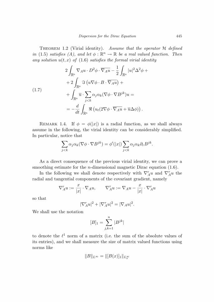
Dispersion for the Dirac Equation 445
Theorem 1.2 (Virial identity). Assume that the operator H definedin (1.5) satisfies (A), and let φ : R
n → R be a real valued function. Thenany solution u(t, x) of (1.6) satisfies the formal virial identity
2∫
Rn
∇Au · D2φ · ∇Au − 12
∫Rn
|u|2∆2φ +
+ 2∫
Rn
(u∇φ · B · ∇Au
)+
+∫
Rn
u ·∑j<k
αjαk(∇φ · ∇Bjk)u =
= − d
dt
∫Rn
(ut(2∇φ · ∇Au + u∆φ)
).
(1.7)
Remark 1.4. If φ = φ(|x|) is a radial function, as we shall alwaysassume in the following, the virial identity can be considerably simplified.In particular, notice that∑
j<k
αjαk(∇φ · ∇Bjk) = φ′(|x|)∑j<k
αjαk∂rBjk.
As a direct consequence of the previous virial identity, we can prove asmoothing estimate for the n-dimensional magnetic Dirac equation (1.6).
In the following we shall denote respectively with ∇rAu and ∇τ
Au theradial and tangential components of the covariant gradient, namely
∇rAu :=
x
|x| · ∇Au, ∇τAu := ∇Au − x
|x| · ∇rAu
so that|∇r
Au|2 + |∇τAu|2 = |∇Au|2.
We shall use the notation
[B]1 =n∑
j,k=1
|Bjk|
to denote the �1 norm of a matrix (i.e. the sum of the absolute values ofits entries), and we shall measure the size of matrix valued functions usingnorms like
‖B‖L∞ = ‖[B(x)]1‖L∞x

446 Federico Cacciafesta
Then we have:
Theorem 1.3 (Smoothing estimates). Let n ≥ 4. Let the operator Hdefined in (1.5) satisfies assumption (A). Let B = DA − DAt = B1 + B2
with B2 ∈ L∞, and assume that
|Bτ (x)| ≤ C1
|x|2 ,12[∂rB(x)]1 ≤ C2
|x|3(1.8)
for all x ∈ Rn and for some constants C1, C2 such that(
94
)C2
1 + 3C2 ≤ (n − 1)(n − 3)(1.9)
Assume moreover that
C0 = ‖|x|2B1‖L∞(Rn) <(n − 2)2
4.
Finally, in the massless case restrict the choice to B1 = B, B2 = 0 in theabove assumptions.
Then for all f ∈ L2 the following smoothing estimate holds
supR>0
1R
∫ +∞
−∞
∫|x|≤R
|eitHf |2dxdt � ‖f‖2L2 .(1.10)
Remark 1.5. As in [13] and [3], a sharper estimate can be proved ifinequality (1.9) is strict, but we won’t deal with the details of this aspecthere.
The limitation to n ≥ 3 space dimensions is intrinsic in the multipliermethod; low dimensions n = 1, 2 require a different approach (see e.g. [4] fora general result in dimension 1). In the present paper we shall only deal withthe case n ≥ 4, the 3-dimensional case being exaustively discussed in [3].Notice that, as it often occurs, the three dimensional case yields differenthypothesis on the potential, being slightly different the multiplicator thatone needs to consider.
A natural application of the smoothing estimate (1.10) is to deriveStrichartz estimates for the perturbed flow eitHf , both in the massless andmassive case. Our concluding result is the following:
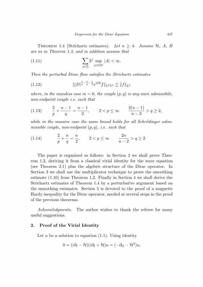
Dispersion for the Dirac Equation 447
Theorem 1.4 (Strichartz estimates). Let n ≥ 4. Assume H, A, B
are as in Theorem 1.3, and in addition assume that∑j∈Z
2j sup|x|∼=2j
|A| < ∞.(1.11)
Then the perturbed Dirac flow satisfies the Strichartz estimates
‖|D|1q− 1
p− 1
2 eitHf‖LpLq � ‖f‖L2(1.12)
where, in the massless case m = 0, the couple (p, q) is any wave admissibile,non-endpoint couple i.e. such that
2p
+n − 1
q=
n − 12
, 2 < p ≤ ∞ 2(n − 1)n − 3
> q ≥ 2,(1.13)
while in the massive case the same bound holds for all Schrodinger adim-missible couple, non-endpoint (p, q), i.e. such that
2p
+n
q=
n
2, 2 < p ≤ ∞ 2n
n − 2> q ≥ 2.(1.14)
The paper is organized as follows: in Section 2 we shall prove Theo-rem 1.2, deriving it from a classical virial identity for the wave equation(see Theorem 2.1) plus the algebric structure of the Dirac operator. InSection 3 we shall use the multiplicator technique to prove the smoothingestimate (1.10) from Theorem 1.2. Finally in Section 4 we shall derive theStrichartz estimates of Theorem 1.4 by a perturbative argument based onthe smoothing estimates. Section 5 is devoted to the proof of a magneticHardy inequality for the Dirac operator, needed at several steps in the proofof the previous theorems.
Acknowledgments. The author wishes to thank the referee for manyuseful suggestions.
2. Proof of the Virial Identity
Let u be a solution to equation (1.1). Using identity
0 = (i∂t −H)(i∂t + H)u = (−∂tt −H2)u,
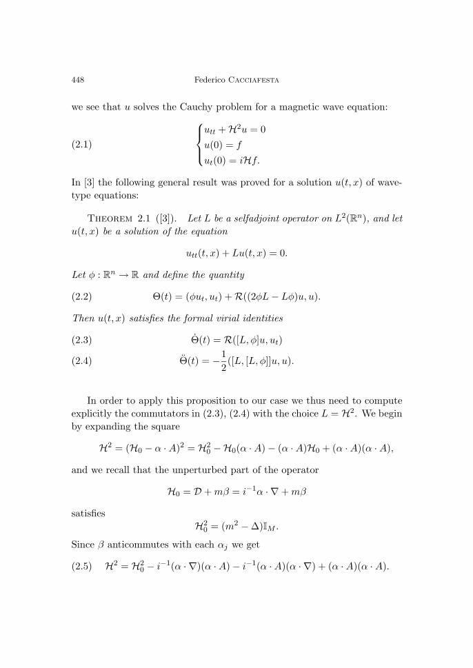
448 Federico Cacciafesta
we see that u solves the Cauchy problem for a magnetic wave equation:utt + H2u = 0
u(0) = f
ut(0) = iHf.
(2.1)
In [3] the following general result was proved for a solution u(t, x) of wave-type equations:
Theorem 2.1 ([3]). Let L be a selfadjoint operator on L2(Rn), and letu(t, x) be a solution of the equation
utt(t, x) + Lu(t, x) = 0.
Let φ : Rn → R and define the quantity
Θ(t) = (φut, ut) + R((2φL − Lφ)u, u).(2.2)
Then u(t, x) satisfies the formal virial identities
Θ(t) = R([L, φ]u, ut)(2.3)
Θ(t) = −12([L, [L, φ]]u, u).(2.4)
In order to apply this proposition to our case we thus need to computeexplicitly the commutators in (2.3), (2.4) with the choice L = H2. We beginby expanding the square
H2 = (H0 − α · A)2 = H20 −H0(α · A) − (α · A)H0 + (α · A)(α · A),
and we recall that the unperturbed part of the operator
H0 = D + mβ = i−1α · ∇ + mβ
satisfiesH2
0 = (m2 − ∆)IM .
Since β anticommutes with each αj we get
H2 = H20 − i−1(α · ∇)(α · A) − i−1(α · A)(α · ∇) + (α · A)(α · A).(2.5)
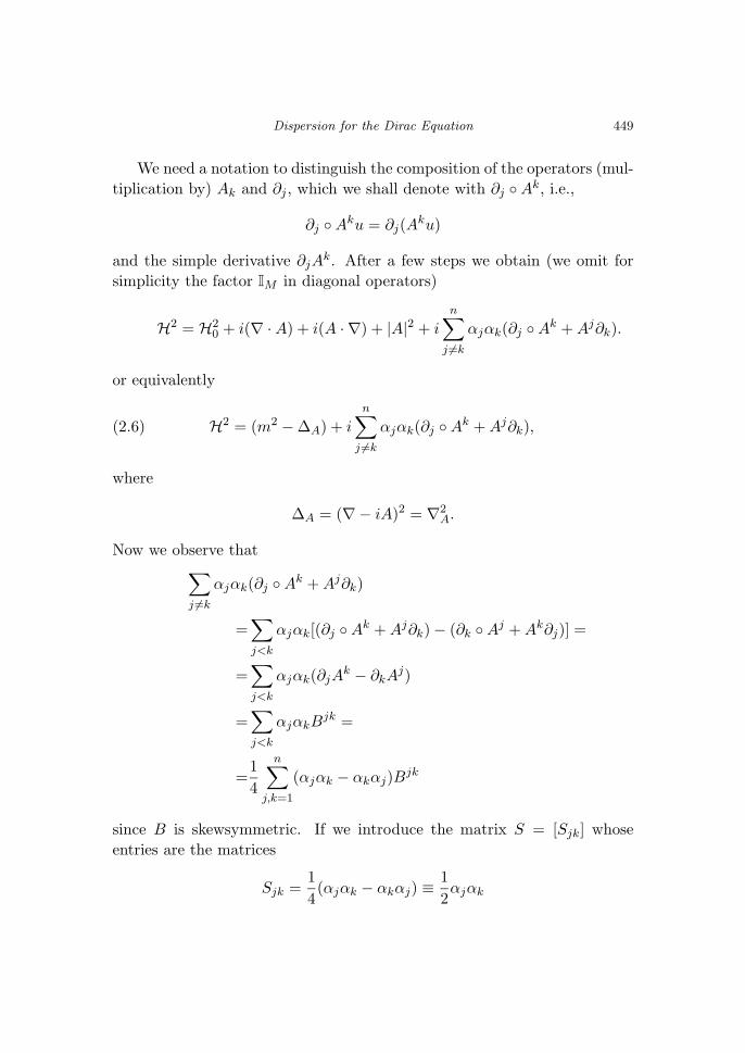
Dispersion for the Dirac Equation 449
We need a notation to distinguish the composition of the operators (mul-tiplication by) Ak and ∂j , which we shall denote with ∂j ◦ Ak, i.e.,
∂j ◦ Aku = ∂j(Aku)
and the simple derivative ∂jAk. After a few steps we obtain (we omit for
simplicity the factor IM in diagonal operators)
H2 = H20 + i(∇ · A) + i(A · ∇) + |A|2 + i
n∑j �=k
αjαk(∂j ◦ Ak + Aj∂k).
or equivalently
H2 = (m2 − ∆A) + in∑
j �=k
αjαk(∂j ◦ Ak + Aj∂k),(2.6)
where
∆A = (∇− iA)2 = ∇2A.
Now we observe that∑j �=k
αjαk(∂j ◦ Ak + Aj∂k)
=∑j<k
αjαk[(∂j ◦ Ak + Aj∂k) − (∂k ◦ Aj + Ak∂j)] =
=∑j<k
αjαk(∂jAk − ∂kA
j)
=∑j<k
αjαkBjk =
=14
n∑j,k=1
(αjαk − αkαj)Bjk
since B is skewsymmetric. If we introduce the matrix S = [Sjk] whoseentries are the matrices
Sjk =14(αjαk − αkαj) ≡
12αjαk
450 Federico Cacciafesta
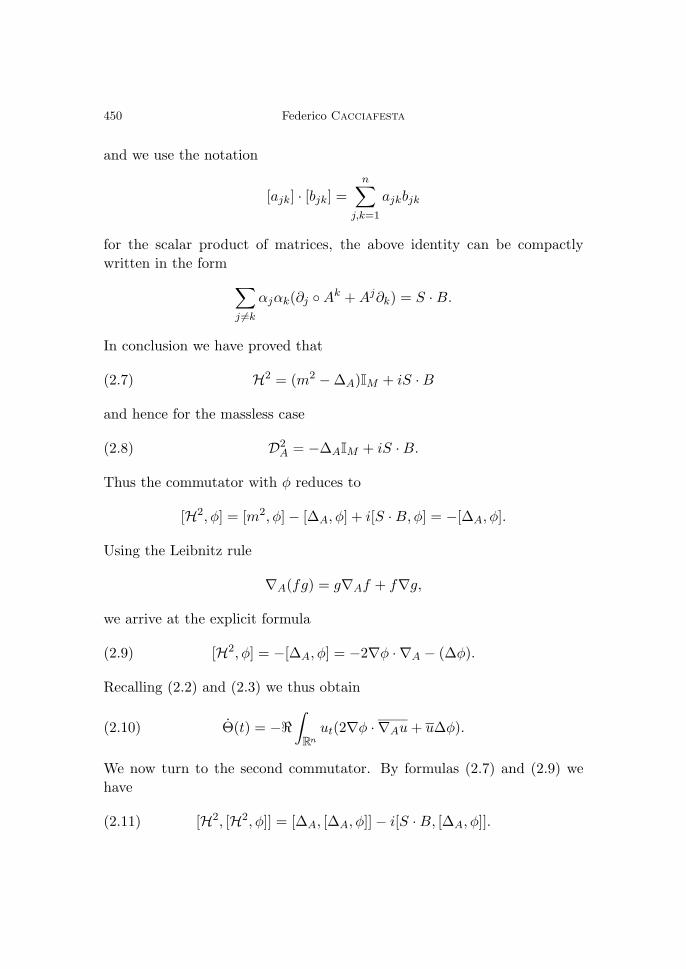
and we use the notation
[ajk] · [bjk] =n∑
j,k=1
ajkbjk
for the scalar product of matrices, the above identity can be compactlywritten in the form ∑
j �=k
αjαk(∂j ◦ Ak + Aj∂k) = S · B.
In conclusion we have proved that
H2 = (m2 − ∆A)IM + iS · B(2.7)
and hence for the massless case
D2A = −∆AIM + iS · B.(2.8)
Thus the commutator with φ reduces to
[H2, φ] = [m2, φ] − [∆A, φ] + i[S · B, φ] = −[∆A, φ].
Using the Leibnitz rule
∇A(fg) = g∇Af + f∇g,
we arrive at the explicit formula
[H2, φ] = −[∆A, φ] = −2∇φ · ∇A − (∆φ).(2.9)
Recalling (2.2) and (2.3) we thus obtain
Θ(t) = −∫
Rn
ut(2∇φ · ∇Au + u∆φ).(2.10)
We now turn to the second commutator. By formulas (2.7) and (2.9) wehave
[H2, [H2, φ]] = [∆A, [∆A, φ]] − i[S · B, [∆A, φ]].(2.11)
Dispersion for the Dirac Equation 451
The first commutator is well known and was computed e.g. in [7]; takingformula (2.19) there (with V ≡ 0) we obtain
(u, [∆A, [∆A, φ]]u) = 4∫
Rn
∇AuD2φ∇Au −∫
Rn
|u|2∆2φ +(2.12)
+ 4∫
Rn
u∇φBτ · ∇Au.
By (2.9) the last term in (2.11) becomes
[S · B, [∆A, φ]] = 2[S · B,∇φ · ∇A] =
= 2(S · B∇φ · ∇A −∇φ · ∇AS · B) =
=∑j<k
αjαkBjk∇φ · ∇A −∇φ · ∇A
∑j<k
αjαkBjk =
=∑j<k
αjαk[Bjk,∇φ · ∇A] =
= −∑j<k
αjαk(∇φ · ∇Bjk).(2.13)
Identity (1.7) then follows from (2.4), (2.10), (2.11), (2.12) and (2.13).
3. Smoothing Estimates
We shall use the following radial multiplier (for a detailed descriptionsee [13], [3]):
φR(x) = φ(x) + ϕR(x)(3.1)
whereφ(x) = |x|
for which we have
φ′(r) = 1, φ′′(r) = 0, ∆2φ(r) = −(n − 1)(n − 3)r3
with the notation r = |x|, and ϕR is the rescaled ϕR(r) = Rϕ0(r
R), of the
multiplier
ϕ0(r) =∫ r
0ϕ′(s)ds(3.2)
452 Federico Cacciafesta
where
ϕ′0(r) =
{n−12n r, r ≤ 1
12 − 1
2nrn−1 , r > 1(3.3)
and so
ϕ′′0(r) =
{n−12n , r ≤ 1n−12nrn , r > 1.
Thus we have
ϕ′R(r) =
{(n−1)r2nR , r ≤ R
12 − Rn−1
2nrn−1 , r > R(3.4)
ϕ′′R(r) =
{1R
n−12n , r ≤ R
1R
Rn(n−1)2nrn , r > R
.(3.5)
∆2ϕR = −n − 12R2
δ|x|=R − (n − 1)(n − 3)2r3
χ[R,+∞).(3.6)
Notice that ϕ′R, ϕ′′
R, ∆ϕR ≥ 0 and moreover supr≥0
ϕ′(r) ≤ 12.
Thus it’s easy to show the bounds for the derivatives of the perturbedmultiplier
supr≥0
φ′R ≤ 3
2, ∆φR ≤ n
r.(3.7)
We separate the estimates of the LHS and the RHS of (1.7)
Estimate of the RHS of (1.7)Consider the expression∫
Rn
ut(2∇φ · ∇Au + u∆φ) = (ut, 2∇φ · ∇Au + u∆φ)L2
appearing at the right hand side of (1.7). Since u solves the equation wecan replace ut with
ut = −iHu = −imβu − iDAu.
Dispersion for the Dirac Equation 453
By the selfadjointess of β it is easy to check that
[−im(βu, 2∇φ · ∇Au) − im(βu,∆φu)] = 0
so that
[(ut, 2∇φ · ∇Au + u∆φ) = 2I(DAu,∇φ · ∇Au)] + I(DAu, ∆φu)
and by Young inequality we obtain∣∣∣∣(∫Rn
ut(2∇φ · ∇Au + u∆φ))∣∣∣∣ ≤ 3
2‖DAu‖2
L2 + ‖∇φ · ∇Au‖2L2 +(3.8)
+12‖u∆φ‖2
L2 .
Now we put in (3.8) the multiplicator φ defined in (3.1). From the bound-edness of ϕ and the magnetic Hardy inequality (5.2) we have, with thechoice ε = (n − 2)2 − 4C0 which is positive in virtue of the assumptionC0 < (n − 2)2/4,
‖∇φ · ∇Au‖2L2 ≤ 3
21
(n − 2)2 − 4C0‖DAu‖2
L2 .(3.9)
The third term in (3.8) can be estimated again using Hardy inequality with
‖u∆φ‖2L2 ≤ 4n
(n − 2)2 − 4C0‖DAu‖2
L2 .(3.10)
Summing up, by (3.8), (3.9) and (3.10) we can conclude∣∣∣∣(∫Rn
ut(2∇φ · ∇Au + u∆φ))∣∣∣∣ ≤ c(n)‖DAu‖2
L2 .(3.11)
Estimate of the LHS of (1.7)We shall make use of the following identity, that holds in every dimen-
sion:
∇AuD2φ∇Au =φ′(r)
r|∇τ
Au|2 + φ′′(r)|∇rAu|2.(3.12)
454 Federico Cacciafesta
For the seek of simplicity, we divide this part in two steps, first consider-ing just the multiplier φ(r) = r, for which the calculations turn out fairlystraightforward, and then perturbating it to φ.
Step 1.With the choice φ(r) = r, by (3.12) we can rewrite the LHS of (1.7) as
follows:
2∫
Rn
|∇τAu|2|x| dx +
(n − 1)(n − 3)2
∫Rn
|u|2|x|3 dx +(3.13)
+2∫
Rn
(uBτ · ∇Au)dx +∫
Rn
u ·∑j<k
αjαk∂rBjku.
The first thing to be done is to prove this quantity to be positive. For whatconcerns the perturbative term, assuming that
|Bτ | ≤C1
|x|2
we have
−∣∣∣∣2 ∫
Rn
(uBτ · ∇Au)dx
∣∣∣∣(3.14)
≥ −2(∫
Rn
|u|2|x|3 dx
) 12(∫
Rn
|x|3|Bτ |2|∇τAu|2dx
) 12
≥ −2C1K1K2,
where
K1 =(∫
Rn
|u|2|x|3 dx
) 12
K2 =(∫
Rn
|∇τAu|2|x| dx
) 12
.
Analogously, assuming∥∥∥∑j<k
αjαk∂rBjk(x)
∥∥∥M×M
≤ 12[∂rB(x)]1 ≤ C2
|x|3
Dispersion for the Dirac Equation 455
(recall that here ‖ · ‖M×M denotes the operator norm of M × M matricesand [·]1 denotes the sum of absolute values of the entries of a matrix) wehave
−
∣∣∣∣∣∣∫
Rn
u ·∑j<k
αjαk∂rBjkudx
∣∣∣∣∣∣ ≥ −∫
|u|2∥∥∥∑
j<k
αjαk∂rBjk
∥∥∥M×M
dx(3.15)
≥ −C2K21
where K1 is as before. Thus we have reached the following estimate
2∫
Rn
|∇τAu|2|x| dx +
(n − 1)(n − 3)2
∫Rn
|u|2|x|3 dx +(3.16)
+2∫
Rn
(uBτ · ∇Au)dx +∫
Rn
u ·∑j<k
αjαk∂rBjku ≥
≥ 2K22 − 2C1K1K2 − C2K
21 +
(n − 1)(n − 3)2
K21 =: C(C1, C2, K1, K2).
As usual, we want to optimize the condition on the constants C1, C2 underwhich the quantity C is positive for all K1, K2. Fixing K2 = 1 and requiringthat (
(n − 1)(n − 3)2
− C2
)K2
1 − 2C1K1 + 2 ≥ 0
we can easily conclude that the resulting condition on the constants is givenby
C21 + 2C2 ≤ (n − 1)(n − 3).(3.17)
Thus, if condition (3.17) is satisfied, we have that the quantity in (3.13) ispositive.
Step 2.We now perturb the multiplier to complete the proof. We thus put the
multiplier φR as defined in (3.1) in the LHS of (1.7), and repeat exactly thesame calculations as in Step 1. Notice that multiplier ϕR with properties
456 Federico Cacciafesta
(3.4)-(3.6) yield the estimate, through (3.12),
2∫
Rn
∇AuD2ϕR∇Au − 12
∫Rn
|u|2∆2ϕR ≥(3.18)
≥ C(n)
(1R
∫|x|≤R
|∇Au|2dx + 2∫ |∇τ
Au|2|x|
)+
+n − 14R2
∫|x|=R
|u|2dσ(x) +(n − 1)(n − 3)
4
∫ |u|2|x|3
for some positive constant C(n). Using now the complete multiplier φR wenotice that estimates (3.14) and (3.15) still hold with the rescaled constantsC1 = 3
2C1, C2 = 32C2, so that we can rewrite (3.16) as follows
1R
∫|x|≤R
|∇Au|2dx + 2∫
Rn
|∇τAu|2|x| dx +(3.19)
+(n − 1)(n − 3)
2
∫Rn
|u|2|x|3 dx +
+2∫
Rn
(uBτ · ∇Au)dx +∫
Rn
u ·∑j<k
αjαk∂rBjku ≥
≥ 1R
∫|x|≤R
|∇Au|2dx + C(C1, C2, K1, K2).
Conditions (1.8)-(1.9) on the potential ensure the positivity of C(C1, C2,
K1, K2)Thus putting all together , taking the supremum over R > 0, integrating
in time and dropping the corresponding nonnegative terms we have reachedthe estimate
2∫ T
−Tdt
∫Rn
∇AuD2φ∇Au − 12
∫ T
−Tdt
∫Rn
|u|2∆2φ +(3.20)
2I∫ T
−Tdt
∫Rn
uφ′Bτ · ∇Au +∫ T
−Tdt
∫Rn
|u|2∑j<k
αjαk(∇φ · ∇Bjk) ≥
≥ supR>0
1R
∫ T
−Tdt
∫|x|≤R
|∇Au|2dx ≥
≥ supR>0
1R
∫ T
−Tdt
∫|x|≤R
|DAu|2dx
Dispersion for the Dirac Equation 457
where in the last step we have used the pointwise inequality |DAu| ≤ |∇Au|.We now integrate in time the virial idetity on [−T, T ], and using (3.20) and(3.11) we obtain
supR>0
1R
∫ T
−Tdt
∫|x|≤R
|DAu|2dx � ‖DAu(T )‖2L2 + ‖DAu(−T )‖2
L2 .(3.21)
Let us now consider the range of DA: from proposition (5.1) we have thatfor C0 < (n − 2)2/4 0 ∈ ker(DA), so ran(DA) is either L2 or it is dense inL2. Fix now an arbitrary g ∈ ran(DA), there exists f ∈ D(DA) = D(H)such that DAf = g. We then consider the solution u(t, x) to the problem{
iut = −mβu + DAu
u(0, x) = f(x)
with opposite mass, and notice that u satisifies (3.21) since no hypothesison the sign of the mass m have been used for it. If we thus apply to thisequation the operator DA we obtain, by the anticommutation rules,{
i(DAu)t = βm(DAu) + DA(DAu)
DAu(0, x) = DAf(x)
or, in other words, the function v = DAu solves the problem{ivt = Hv
v(0, x) = g
so that v = eitHg. Substituting in (3.21) and letting T → ∞ we concludethat, in view of Remark (1.2),
supR>0
1R
∫ +∞
−∞
∫|x|≤R
|eitHg|2 � ‖g‖2L2
that is exactly (1.10) for g ∈ ran(DA), which is as we have noticed dense inL2. Density arguments conclude the proof.
458 Federico Cacciafesta
4. Proof of the Strichartz Estimates
We begin by recalling the Strichartz estimates for the free Dirac flow,both in the massless and in the massive case. They are a direct consequenceof the corresponding estimates for the wave and Klein-Gordon equations:
Proposition 4.1. Let n ≥ 3. Then the following Strichartz estimateshold:
(i) in the massless case, for any wave admissible couple (p, q) (see (1.13))
‖|D|1q− 1
p− 1
2 eitDf‖LpLq � ‖f‖L2 ;(4.1)
(ii) in the massive case, for any Schrodinger admissible couple (p, q) (see(1.14))
‖|D|1q− 1
p− 1
2 eit(D+β)f‖LpLq � ‖f‖L2 .(4.2)
Proof. We restrict the proof to the case n ≥ 4, refering to [3] for anexaustive proof of the 3-dimensional case.
Recalling identity (1.3) we immediately have that u(t, x) = eitDf andv(t, x) = eit(D+β) satisfy the two Cauchy problems
utt − ∆u = 0
u(0, x) = f(x)
ut(0, x) = iDf,
(4.3)
vtt − ∆v + mv = 0
v(0, x) = f(x)
vt(0, x) = i(D + β)f,
(4.4)
and so each component of the M -dimensional vectors u and v satisfy thesame Strichartz estimates as for the n-dimensional wave equation and Klein-Gordon equation respectively. Thus case (i) follows from the standard esti-mates proved in [14] and [17], while case (ii) follows from similar techniques(the details can be found e.g. in the Appendix of [6]). �
Dispersion for the Dirac Equation 459
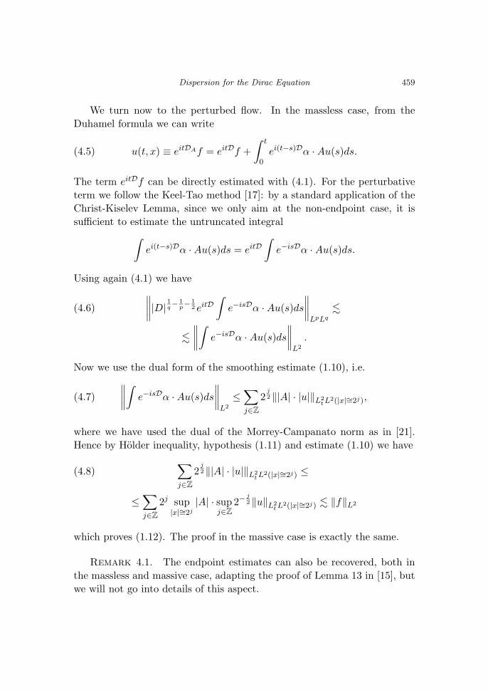
We turn now to the perturbed flow. In the massless case, from theDuhamel formula we can write
u(t, x) ≡ eitDAf = eitDf +∫ t
0ei(t−s)Dα · Au(s)ds.(4.5)
The term eitDf can be directly estimated with (4.1). For the perturbativeterm we follow the Keel-Tao method [17]: by a standard application of theChrist-Kiselev Lemma, since we only aim at the non-endpoint case, it issufficient to estimate the untruncated integral∫
ei(t−s)Dα · Au(s)ds = eitD∫
e−isDα · Au(s)ds.
Using again (4.1) we have∥∥∥∥|D|1q− 1
p− 1
2 eitD∫
e−isDα · Au(s)ds
∥∥∥∥LpLq
�(4.6)
�∥∥∥∥∫
e−isDα · Au(s)ds
∥∥∥∥L2
.
Now we use the dual form of the smoothing estimate (1.10), i.e.∥∥∥∥∫e−isDα · Au(s)ds
∥∥∥∥L2
≤∑j∈Z
2j2 ‖|A| · |u|‖L2
t L2(|x|∼=2j),(4.7)
where we have used the dual of the Morrey-Campanato norm as in [21].Hence by Holder inequality, hypothesis (1.11) and estimate (1.10) we have∑
j∈Z
2j2 ‖|A| · |u|‖L2
t L2(|x|∼=2j) ≤(4.8)
≤∑j∈Z
2j sup|x|∼=2j
|A| · supj∈Z
2−j2 ‖u‖L2
t L2(|x|∼=2j) � ‖f‖L2
which proves (1.12). The proof in the massive case is exactly the same.
Remark 4.1. The endpoint estimates can also be recovered, both inthe massless and massive case, adapting the proof of Lemma 13 in [15], butwe will not go into details of this aspect.
460 Federico Cacciafesta
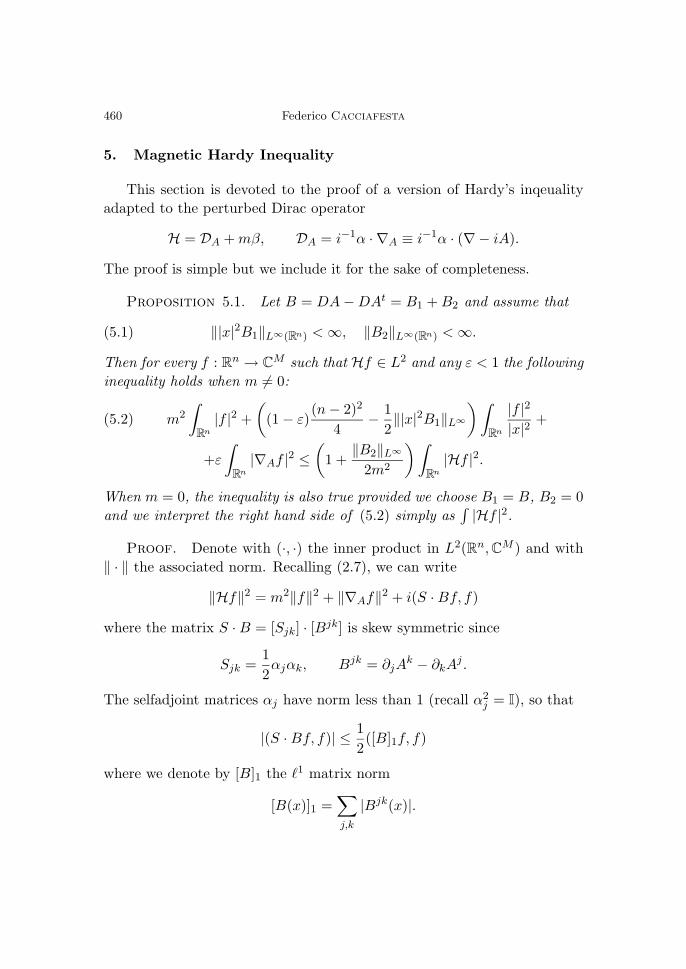
5. Magnetic Hardy Inequality
This section is devoted to the proof of a version of Hardy’s inqeualityadapted to the perturbed Dirac operator
H = DA + mβ, DA = i−1α · ∇A ≡ i−1α · (∇− iA).
The proof is simple but we include it for the sake of completeness.
Proposition 5.1. Let B = DA − DAt = B1 + B2 and assume that
‖|x|2B1‖L∞(Rn) < ∞, ‖B2‖L∞(Rn) < ∞.(5.1)
Then for every f : Rn → C
M such that Hf ∈ L2 and any ε < 1 the followinginequality holds when m = 0:
m2
∫Rn
|f |2 +(
(1 − ε)(n − 2)2
4− 1
2‖|x|2B1‖L∞
) ∫Rn
|f |2|x|2 +(5.2)
+ε
∫Rn
|∇Af |2 ≤(
1 +‖B2‖L∞
2m2
) ∫Rn
|Hf |2.
When m = 0, the inequality is also true provided we choose B1 = B, B2 = 0and we interpret the right hand side of (5.2) simply as
∫|Hf |2.
Proof. Denote with (·, ·) the inner product in L2(Rn, CM ) and with‖ · ‖ the associated norm. Recalling (2.7), we can write
‖Hf‖2 = m2‖f‖2 + ‖∇Af‖2 + i(S · Bf, f)
where the matrix S · B = [Sjk] · [Bjk] is skew symmetric since
Sjk =12αjαk, Bjk = ∂jA
k − ∂kAj .
The selfadjoint matrices αj have norm less than 1 (recall α2j = I), so that
|(S · Bf, f)| ≤ 12([B]1f, f)
where we denote by [B]1 the �1 matrix norm
[B(x)]1 =∑j,k
|Bjk(x)|.
Dispersion for the Dirac Equation 461
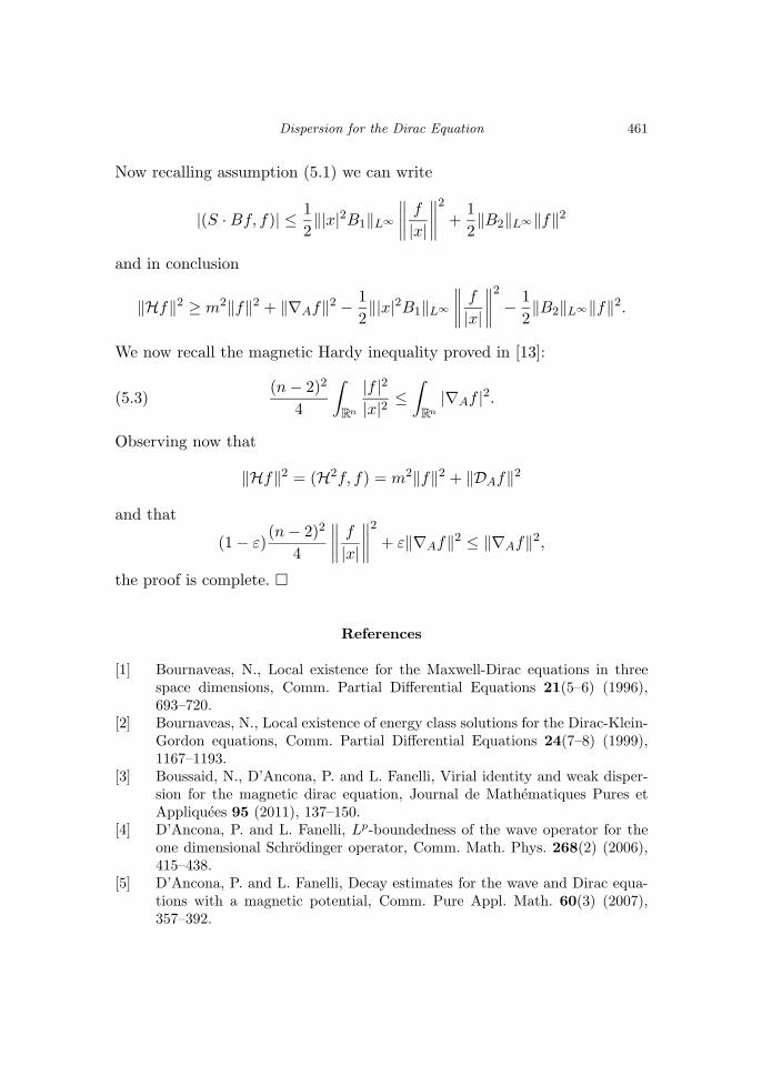
Now recalling assumption (5.1) we can write
|(S · Bf, f)| ≤ 12‖|x|2B1‖L∞
∥∥∥∥ f
|x|
∥∥∥∥2
+12‖B2‖L∞‖f‖2
and in conclusion
‖Hf‖2 ≥ m2‖f‖2 + ‖∇Af‖2 − 12‖|x|2B1‖L∞
∥∥∥∥ f
|x|
∥∥∥∥2
− 12‖B2‖L∞‖f‖2.
We now recall the magnetic Hardy inequality proved in [13]:
(n − 2)2
4
∫Rn
|f |2|x|2 ≤
∫Rn
|∇Af |2.(5.3)
Observing now that
‖Hf‖2 = (H2f, f) = m2‖f‖2 + ‖DAf‖2
and that
(1 − ε)(n − 2)2
4
∥∥∥∥ f
|x|
∥∥∥∥2
+ ε‖∇Af‖2 ≤ ‖∇Af‖2,
the proof is complete. �
References
[1] Bournaveas, N., Local existence for the Maxwell-Dirac equations in threespace dimensions, Comm. Partial Differential Equations 21(5–6) (1996),693–720.
[2] Bournaveas, N., Local existence of energy class solutions for the Dirac-Klein-Gordon equations, Comm. Partial Differential Equations 24(7–8) (1999),1167–1193.
[3] Boussaid, N., D’Ancona, P. and L. Fanelli, Virial identity and weak disper-sion for the magnetic dirac equation, Journal de Mathematiques Pures etAppliquees 95 (2011), 137–150.
[4] D’Ancona, P. and L. Fanelli, Lp-boundedness of the wave operator for theone dimensional Schrodinger operator, Comm. Math. Phys. 268(2) (2006),415–438.
[5] D’Ancona, P. and L. Fanelli, Decay estimates for the wave and Dirac equa-tions with a magnetic potential, Comm. Pure Appl. Math. 60(3) (2007),357–392.

462 Federico Cacciafesta
[6] D’Ancona, P. and L. Fanelli, Strichartz and smoothing estimates of dispersiveequations with magnetic potentials, Comm. Partial Differential Equations33(4–6) (2008), 1082–1112.
[7] D’Ancona, P., Fanelli, L., Vega, L. and N. Visciglia, Endpoint Strichartzestimates for the magnetic Schrodinger equation, J. Funct. Anal. 258(10)(2010), 3227–3240.
[8] D’Ancona, P., Foschi, D. and S. Selberg, Local well-posedness below thecharge norm for the Dirac-Klein-Gordon system in two space dimensions, J.Hyperbolic Differ. Equ. 4(2) (2007), 295–330.
[9] D’Ancona, P., Foschi, D. and S. Selberg, Null structure and almost opti-mal local regularity for the Dirac-Klein-Gordon system, J. Eur. Math. Soc.(JEMS) 9(4) (2007), 877–899.
[10] D’Ancona, P., Foschi, D. and S. Selberg, Null structure and almost optimallocal well-posedness of the Maxwell-Dirac system, Amer. J. Math. 132(3)(2010), 771–839.
[11] Dias, J.-P. and M. Figueira, Global existence of solutions with small initialdata in Hs for the massive nonlinear Dirac equations in three space dimen-sions, Boll. Un. Mat. Ital. B (7) 1(3) (1987), 861–874.
[12] Escobedo, M. and L. Vega, A semilinear Dirac equation in Hs(R3) for s > 1,SIAM J. Math. Anal. 28(2) (1997), 338–362.
[13] Fanelli, L. and L. Vega, Magnetic virial identities, weak dispersion andStrichartz inequalities, Math. Ann. 344(2) (2009), 249–278.
[14] Ginibre, J. and G. Velo, Generalized Strichartz inequalities for the wave equa-tion, In Partial differential operators and mathematical physics (Holzhau,1994), volume 78 of Oper. Theory Adv. Appl., pages 153–160, Birkhauser,Basel, 1995.
[15] Ionescu, A. D. and C. Kenig, Well-posedness and local smoothing of solutionsof Schrodinger equations, Math. Res. Letters 12 (2005), 193–205.
[16] Kalf, H. and O. Yamada, Essential self-adjointness of n-dimensional Diracoperators with a variable mass term, J. Math. Phys. 42(6) (2001), 2667–2676.
[17] Keel, M. and T. Tao, Endpoint Strichartz estimates, Amer. J. Math. 120(5)(1998), 955–980.
[18] Machihara, S., Nakamura, M., Nakanishi, K. and T. Ozawa, EndpointStrichartz estimates and global solutions for the nonlinear Dirac equation,J. Funct. Anal. 219(1) (2005), 1–20.
[19] Machihara, S., Nakamura, M. and T. Ozawa, Small global solutions for non-linear Dirac equations, Differential Integral Equations 17(5–6) (2004), 623–636.
[20] Ozawa, T. and K. Yamauchi, Structure of Dirac matrices and invariants fornonlinear Dirac equations, Differential Integral Equations 17(9–10) (2004),971–982.
[21] Perthame, B. and L. Vega, Morrey-Campanato estimates for Helmholtz equa-tions, J. Funct. Anal. 164(2) (1999), 340–355.
Dispersion for the Dirac Equation 463
[22] Thaller, B., The Dirac equation, Texts and Monographs in Physics, Springer-Verlag, Berlin, 1992.
(Received April 4, 2011)(Revised November 25, 2011)
SAPIENZA — Universita di RomaDipartimento di MatematicaPiazzale A. Moro 2I-00185 Roma, ItalyE-mail: [email protected]