- 1 -

Violations of the Law of One Fee in the Mutual Fund Industry

Michael Cooper, Michael Halling and Michael Lemmon*

March 28, 2013

Keywords: mutual funds, fund fees, price dispersion, price persistence.

JEL Classifications: G10, G11, G23.

* All authors are with the David Eccles School of Business, University of Utah. Halling is also at the Stockholm School of Economics and the Swedish House of Finance. We thank Darwin Choi, James Choi (WFA discussant), Magnus Dahlquist, Amit Goyal, Joseph Halford, Rachel Hayes, Keith Jacob, Stephan Jank (discussant), Dong Lou (discussant), Veronika K. Pool (discussant), Jonathan Reuter, David Robinson, Norman Schuerhoff, Mark Seasholes, Laura Starks, Paul Tetlock and Charles Trzcinka. We also thank participants of the CEPR ESSFM meetings (2011, asset pricing week), the Northern Finance Association Meetings (2011), the 12th FBI Symposium in Karlsruhe, the 2012 WFA meetings and seminar participants at HEC Lausanne, the Institute of Advanced Studies in Vienna, KAIST, Nanyang Tech University, the Shanghai Advanced Institute of Finance, the University of Arizona, the University of Colorado, the University of Montana and VU University Amsterdam for their comments. An earlier version of this paper was titled “Fee Dispersion and Persistence in the Mutual Fund Industry”.

- 2 -

Violations of the Law of One Fee in the Mutual Fund Industry

Abstract

In competitive markets, similar products should have similar prices. We apply this concept to mutual funds.

We examine the residuals from regressions of fees (annual expenses and 12b-1 fees) on important fund

characteristics, essentially allowing us to compare the fees of “identical” funds. We present striking new evidence

of systematic differences in residual fees across all US equity funds. We find that the average spread in residual

fees across funds over the sample is approximately 2.3%. The dispersion in fees has not decreased over time,

despite the fact that significant numbers of new funds have entered and the aggregate amount of assets under

management has increased substantially. An investor purchasing similar lower fee funds would have

outperformed an investor purchasing higher fee funds by approximately 32% over our sample. We test a number

of hypotheses to explain our results including a random fee, competition, service, captive investor, and strategic

fee setting hypothesis, and are able to explain only a small portion of the spread in residual fees. Surprisingly, a

main determinant of fees is the initial fee set by a fund, which varies little over time. Overall, our evidence is

largely inconsistent with a competitive market for mutual funds.

- 3 -

1. Introduction

A large literature exists that attempts to explain why similar products sell for different prices. For example,

Lach (2002) documents considerable price dispersion for similar refrigerators, chicken, coffee, and flour.1 He

concludes that because stores change their pricing on a regular basis, consumers cannot learn which stores are the

low cost sellers, and as a consequence, price dispersion persists.

In the mutual fund markets, Elton, Gruber, and Busse (2004) document price dispersion of more than 2% per

year for essentially identical S&P500 index funds.2 They conclude that a combination of the inability to arbitrage

(i.e., one cannot short sell open-ended mutual funds) and uninformed investors is sufficient to have the law of one

price fail in the S&P500 index fund market. Other papers, focusing on sub-categories of funds, also provide

evidence of differential prices being charged for funds with similar characteristics.3

In contrast, other papers suggest that the mutual fund markets are more or less competitively priced. For

example, Khorana, Servaes, and Tufano (2009) examine mutual fund fees in 18 countries and find that most of the

cross-sectional dispersion in fees can be explained by economic variables, such as investment objective, sponsor,

national characteristics, and levels of investor protection.4 More recently, Wahal and Wang (2011) provide

evidence that incumbents with high overlap in their portfolio holdings with entrants subsequently engage in price

competition by reducing their management fees. In addition, they also find evidence that incumbents with higher

portfolio overlap with entrants have lower future fund inflows. They conclude that the mutual fund market has

“evolved into one that displays the hallmark features of a competitive market.” Overall, while the existing

literature provides evidence of price dispersion in specific areas of the mutual fund market, there is little existing

1 See also Bakos (2001), Brown and Goolsbee (2002), Brynjolfsson and Smith (2000), Nakamura (1999), Pratt, et al. (1979), Scholten and Smith (2002), and Sorensen (2000). 2 See also Hortacsu and Syverson (2004). 3 See also Elton, Gruber, and Rentzler (1989) who find that public commodity funds exist that underperform the risk free rate and Christoffersen and Musto (2002) who find a wide dispersion in fees across similar money market funds. 4 See also Khorana and Servaes (2009) who examine determinants of mutual fund family market share. They document that fund families that charge lower style-adjusted fees relative to other families and families whose expense ratios decline as the fund family size grows have higher market share. They also find that families whose expenses are above the mean increase their market share when they lower their expenses.

- 4 -

evidence on how widespread the phenomenon is or on how it has changed over time given the dramatic growth in

the mutual fund market.

In this paper, we examine if the “law of one fee” (the idea that if the mutual fund market is more-or-less

competitive, then similar mutual funds, as measured by important fund characteristics, should have roughly

similar fees) holds. We examine the residuals from regressions of fees (annual expenses and 12b-1 fees) on

important fund characteristics, essentially allowing us to compare the fees of “identical” funds. We present new

evidence of systematic differences in residual fees across all US equity funds. Specifically, we find that the

average spread in residual fees (between the 1st and 99th percentile) across all funds over the sample is 2.34%.

More interestingly, the dispersion in residual fees has not decreased over time, despite the fact that significant

numbers of new funds have entered and the aggregate amount of assets under management has increased

substantially over time. Our results hold for both the largest total net asset (TNA) funds as well as the smaller

TNA funds; the average spread in residual fees is 2.88% for the smallest quintile of TNA funds and is 1.18% for

the largest quintile of funds. 5 In fact, for the largest quintile funds, representing 82% of the market value of our

sample, the spread in residual fees has actually increased from 1990 to 2009, evidence that is potentially difficult

to reconcile with a competitive market for mutual funds.

We examine the implications of our findings for investors. Based on raw (residual) fees, an investor

purchasing the lowest fee funds would have earned compounded abnormal returns 67% (32%) higher than an

investor purchasing the most expensive funds. As a basis for comparison, the compounded differences in fees

(residual fees) over the period were 90% (64%). Thus, while the difference in abnormal returns between high fee

and low fee funds is less than the cumulative difference in fees, it appears that investors bear significant costs

from investing in high fee mutual funds that are not recouped through higher performance of these funds.

We explore various explanations for the large price dispersion across similar funds. We first note that

controlling for product characteristics that investors are likely to care about when purchasing a fund, such as

5 Our results are robust to multiple variations in the models used to estimate residual fees, variations in residual estimation techniques (including the use of stochastic frontier models), aggregation of share classes, and the use of before-fee returns in estimating residual fees.

- 5 -

search costs, service levels, fund size, retail versus institutional funds, fund age, fund flows, fund portfolio

characteristics (i.e., lagged performance and style betas) explains about 44% of the dispersion in raw fees, leaving

a sizable unexplained dispersion in fees.

We test various hypotheses to explain this dispersion. We first test a “random fee” hypothesis (Lach (2002)

and others) which posits that mutual funds engage in frequent changes in their fees, resulting in fund consumers

not being able to easily identify low fee funds, which in turn results in persistent price dispersion. We add a

random fee change variable (based on the number of fee increases and decreases for a given fund) to our fee

regressions and find that funds that change their fees more often charge higher fees, consistent with theory. We

next examine the residuals from the regressions that include the random fee change variable and find a very small

or even zero effect on residual fee spreads. Thus, despite the significance of the random fee change variable in

fee regressions, the overall economic effect on the fee residuals is small, suggesting that the random fee

hypothesis does not explain our results.

Given the small effect on residual fees from fee switching, we perform additional tests to better understand

fee randomization in the mutual fund industry. We estimate transition probabilities among low and high fee funds

and find evidence inconsistent with a random fee explanation. For both raw and residual fees, low fee funds tend

to stay low and high fee funds tend to stay high. It is very rare that high fee funds become low or that low fee

funds become high.6 Given that there is scant evidence for fee switching over time, we examine the role of a

fund’s initial fee in explaining the cross-section of raw fees. As mentioned above, regression specifications that

include standard determinants of fund fees obtain average adjusted R-squareds of approximately 44%. When we

add a fund’s initial fee to the regressions, the R-squareds of the regressions increase up to 70%. To shed further

light on this issue we study the determinants of initial fees. We find that initial fees are higher for funds that enter

with smaller size, smaller fund families, fund families that charge higher average fees, and for families that have a

higher dispersion of fees within the fund family. We also find that factor returns (i.e., the market risk premium,

SMB, HML, and UMD) are consistently negatively related to first fees. A potential interpretation is that in

6 Liang (2000), among others, documents similar evidence concerning a lack of fee changes in the hedge fund industry.

- 6 -

periods when factors are doing poorly, actively managed funds can charge excess fees. Interactions between

factor returns and betas are consistently positively related to first fees, implying that in situations when funds are

founded in styles that have been successful in the past, higher fees are charged. Thus, first fees are strongly related

to a fund’s lifetime expense ratio.

We test four more hypotheses in an attempt to gain a better understanding of how funds set fees and how fees

evolve over time. We test the competition hypothesis which predicts that funds that deal with more competing

fund should have lower fees. For example, Wahal and Wang (2011) show that when existing funds face

competition from new, similar funds, the existing funds lower their fees to better compete with the upstart funds.

We regress fees on variables designed to capture the amount of competition that each fund is facing. We find that

the number of competing funds is significantly negatively related to and the average fee of the competitors is

significantly positively related to a fund’s fee, supporting the competition hypothesis. Lastly, we test if the

competition hypothesis can explain much of the spread in fee residuals. For the full sample and the sample of

largest funds, there are only small drops in the residuals. For the smallest funds, there are larger drops, ranging

from 15 to 77 basis points. However, even after controlling for competition, the small-fund residual fee spread is

economically large. Thus, competition appears to play a role in the setting of mutual fund fees, especially so for

smaller TNA funds, but does not drive away the large spreads in residual fees.

Next, we test the fund family service hypothesis. Hortacsu and Syverson (2004), Collins (2005) and others

have suggested that variation in services, such as financial advice or complementary investment instruments, may

explain fee variation. Assuming that large fund families offer better service, we find that funds that are part of a

family with more than 100 funds charge, on average, an extra 6 to 27 basis points in fees, but controlling for large

fund families (using fund family fixed effects in the fee regressions) does not alter our finding of large spreads in

residual fees. Our results do not appear to be explained by differences in the services offered by funds.

Another hypothesis we test is the captive investor hypothesis. We examine if funds that are likely to inhibit

easy investor exit (thus creating captive investors) are the funds with high residual fees. We define captive

investors two ways. First, we define funds that are “easy-in, hard-out” funds. These are funds that spend more

- 7 -

than other funds on advertising and have higher back-end loads. Second, using a subsample of funds with high

flow autocorrelations, we examine the fees of funds that are likely to be held within pension funds, thus not

allowing for easy investor exit. We find evidence consistent with the captive investor hypothesis: high fee funds

have higher back-end loads and spend more on advertising than do lower fee funds. Also, high fee funds have

higher positive autocorrelation of flows than do lower fee funds. Finally, we add flow autocorrelation and a

dummy for “easy-in, hard-out” funds to the fee regressions and examine their effects on the residual fee spreads.

Although these measures of captive investors result in significant positive regression coefficients, consistent with

theory, they are not able to explain or substantially reduce the level of residual fee dispersion.

The last hypothesis we test is the strategic fee setting hypothesis (SFSH). Christoffersen and Musto (2002)

and Gil-Bazo and Ruiz-Verdu (2008) show that performance sensitive investors withdraw assets from poorly

performing funds leaving only performance insensitive investors as holders of the funds’ shares. Funds respond to

the fact that the fund flows of the remaining investors are not sensitive to fund performance by raising fees. To

test the SFSH, we estimate each fund’s flow-performance sensitivity and examine how it relates to fees. The

SFSH suggests that funds whose investors are more performance sensitive should have lower fees. In regressions

of fees on flow-performance sensitivity and other controls, we find a positive and significant coefficient on flow-

performance sensitivity, inconsistent with the predictions from the SFSH. Finally, we examine if residual fee

spreads decrease once we control for flow-performance sensitivity and find basically no change at all.

In a final step, we analyze the combined effect of the previously discussed hypotheses on mutual fund fees

and spreads of residual fees. In a multiple regression of fees on the variables designed to capture our five

hypotheses, all coefficients keep the signs that they showed when we controlled for each individually (i.e., fees

increase as fees of competing funds, random fee changes, flow-performance sensitivity, and flow autocorrelation

increases, and fees decrease as the number of competing funds increase) and, with the exception of the flow

autocorrelation variable in the early part of the sample, all coefficients remain statistically significant. In order of

importance, the fees of competing funds is most important, fund flow autocorrelation is next important, and

random fee changes are third most important in determining fund fees. Finally, we estimate the joint effect of our

- 8 -

hypotheses on the residual fee distribution. Controlling for all hypotheses results in residual fee distribution break

points that are only slightly less than the base case.

Overall, our results raise two important questions. First, given that fees are important sources of

underperformance, why do funds not manage their fees more actively?7 Second, why do investors not learn to

distinguish cheap from expensive funds? A potential explanation for these questions is that investors may have

difficulty learning about the quality of funds, which allows different funds to charge different prices for delivering

a similar product. This, however, does not necessarily mean that investors are unable or unwilling to learn. Carlin

and Manso (2011) address this issue in a dynamic theoretical model and show that funds may optimally react to

investor learning by increasing the level of obfuscation (i.e., by making it harder for investors to learn). They

argue, however, that an increase in competition should lower the incentives for obfuscation and, thus, should

enable investors to learn more quickly.8 Overall, we conclude that the large dispersion in prices for similar funds

is inconsistent with a competitive market for mutual funds.

The remainder of the paper is organized as follows. In Section I we describe the data used in our analysis and

describe the characteristics of high and low fee funds. In Section II we present results that document price

dispersion in the residual fee distribution of funds and perform tests to quantify the economic effects of fee

dispersion for fund investors. In Section III we test various hypotheses to explain the apparent large mispricing of

funds. Section IV concludes.

2. Data

2.1 Sample Construction

The sample selection follows Pastor and Stambaugh (2002). Accordingly, we select only domestic equity

funds and exclude all funds not investing primarily in equities such as money market or bond funds. In addition,

7 In related work, there are several papers that develop theoretical models of the mutual fund industry, including endogenous fee setting. Nanda, Narayanan and Warther (2000) concentrate on the structure of mutual funds, i.e., on the combination of loads and fees. Das and Sundaram (2002) compare fulcrum fees to incentive fees. Pastor and Stambaugh (2010) use their model to study the aggregate size of the active management mutual fund market. 8 Ellison and Wolitzky (2012) develop a static model of obfuscation and find that competition might actually lead to more confiscation, increased search costs and more price dispersion.

- 9 -

we exclude international funds, global funds, balanced funds, flexible funds, and funds of funds. The ICDI

classification codes that were used by Pastor and Stambaugh (2002) are, however, no longer available. Thus, we

follow Bessler et al. (2008) who use a combination of Lipper codes, Wiesenberger codes and Strategic Insight

codes to identify domestic equity funds. Table A in the Appendix lists the specific codes that we use to identify

the funds in our sample.

In short, the above screens result in our sample focusing on active and passive US domestic equity funds.

Our sample includes approximately 35% of all funds covered in the CRSP Mutual Fund Database (our sample

consists of a total of 13,817 funds while the CRSP Mutual Fund Database universe has approximately 40,000

funds). As measured by total net assets, our sample covers approximately 32% of the cumulative net assets

represented in the database. The sample period spans 1963 to 2008 and the data frequency is yearly, as we focus

on fund fees.9

2.2 Descriptive Statistics

Table 1 Panel A reports summary statistics of our fund sample. Details of the variable construction can be

found in Table B in the Appendix. Throughout the paper we distinguish between a pre-1999 (up to and including

1998) and a post-1999 (including 1999) sample because several important variables such as fund family

information and flags for institutional funds became available in the CRSP Mutual Fund Database in 1999.

The descriptive statistics show the dramatic increase in mutual funds over the past 30 years. In the pre-1999

sample the mean number of funds per year is 545, while it increases to 5562 in the post-1999 sample. Note that

the mean fund size (mtna) also increases from 436 Million USD pre-1999 to 464 Million USD post-1999. Thus,

the mutual fund industry has experienced a considerable increase in assets under management.

Intuitively, given more funds and thus presumably increased competition, we would have expected to find

that the rapid expansion of the mutual fund industry was also accompanied by a decrease in average expense

ratios – but this is not the case. Average annual expense ratios (exp_ratio) and initial annual expense ratios of

9 Quarterly data on fees and other fund characteristics is only available starting in 1999.

- 10 -

entering funds (first_exp_ratio) both increased, from 1.3% to 1.4% and 1.3% to 1.5%, respectively. It is also

interesting to observe that average yearly changes of expense ratios (Δ(exp_ratio)) are on average zero (with a

tiny standard deviation of 18 bps pre-1999 and 9 bps post-1999).

The average performance (yalpha) of our sample funds, as measured by annual four-factor alphas (Carhart

(1997)), is slightly negative, consistent with Carhart (1997) and others who show that funds do not earn positive

abnormal returns net of fees. The average fund, over both time periods, has a market beta (beta_mkt) that is

slightly less than 1, a small, negative exposure to HML (beta_hml), and small positive exposures to SMB

(beta_smb) and UMD (beta_umd). After 1999, funds load more on the market, and less on HML, SMB, and

UMD, consistent with an aggregate strategy shift to market indexing. The four-factor model works very well on

average in explaining fund returns, yielding R-squareds (r_squared) of 84% and 87%, respectively.

Panel B (pre-1999 sample) and Panel C (post-1999 sample) of Table 1 report summary statistics by expense

ratio deciles. Each year we split all funds into deciles by their expense ratios and then report contemporaneous

means and standard deviations of fund characteristics.

Average expense ratios of decile 10 exceed those of decile 1 by 2.1%, in both the pre-1999 and post-1999

periods. In the pre-1999 sample, average expense ratio changes are most negative (-6 bps) in decile 1 and most

positive (15 bps) in decile 10. These mean changes become even smaller in the post-1999 sample: funds in the

bottom expense ratio decile decrease their fees on average by 1 bps in the same year, while funds in the top decile

increase their fees on average by 3 bps in the same year.

All of the fund performance variables decrease monotonically by expense ratio deciles. The spread in yearly

four-factor alphas, for example, equals 2.7% (decile 1 alpha is -0.12% and decile 10 is -2.79%) pre-1999 and 2%

(decile 1 alpha is 0.1% and decile 10 is -1.86%) post-1999, which in both cases basically equals the spread in

expense ratios. Thus, these simple descriptive statistics suggest that funds with higher expense ratios on average

underperform their cheaper competitors by approximately their expense ratios (consistent with Berk and Green

(2004)).

- 11 -

We also find that average funds in decile 1 are much larger than average funds in decile 10 suggesting that

economies of scale play a role for expense ratios. The average fund in decile 1 is approximately 1.5 Billion USD

larger in both the pre-1999 and post-1999 periods than the average fund in expense ratio decile 10. We also find

that funds which are part of a larger fund family on average have lower fees.10 This result is potentially consistent

with an economies-of-scope argument. Moreover, we also find that institutional funds and ETFs have lower fees,

as one would expect.

Finally, Panel D of Table 1 shows time-series means of cross-sectional correlations between fund

characteristics. These correlations are consistent with our previous interpretations of patterns between expense

ratio deciles and other fund characteristics. In general, none of these correlations seem to be high enough to cause

worries about multi-collinearity problems in the subsequent multivariate analysis.

Of course, the most important limitation of this univariate analysis from Table 1 is that it ignores that

expense ratios may reflect different fund strategies and characteristics. This is something that we will explore in

more detail in later sections of the paper. These simple summary statistics, however, already suggest that to some

extent, expense ratios can be explained by economic determinants. For example, funds’ risk characteristics seem

to be correlated with expense ratios: more expensive funds tend to exhibit returns similar to small cap, value, and

momentum styles of investing (as judged by their loadings on the SMB, HML, and UMD factors, respectively).

Similarly, the average R-squared of the four-factor model decreases as we move from decile 1 to decile 10,

suggesting that the managers of the higher fee funds may be following “unique” strategies, likely in an attempt to

outperform. However, these managers also trade much more (the turnover (turn_rat) is much higher for the high

fee funds relative to the low fee funds), which may contribute to their low return performance. Overall, these

patterns between risk characteristics and expense ratios are intuitive and suggest that expensive funds do follow,

at least to some extent, more active strategies, load more aggressively on individual risk factors and also

implement strategies that go beyond the standard risk factors.

10 This pattern, however, is non-monotonic across raw fee deciles. In later cross-sectional tests we find that large families actually tend to charge greater fees.

- 12 -

3. The Pricing of Mutual Funds

3.1 Residual Fee Estimation

Our goal is to compare prices (annual management expenses and 12b-1 fees) across funds. Of course, not all

funds are the same and differences in fund characteristics might justify price differences. Thus, we follow Lach

(2002) and Sorensen (2000) to control for fund heterogeneity. As controls we use the standard fund characteristics

that have been shown to be important in determining fund fees (e.g., see Gil-Bazo and Ruiz-Verdu (2009) and

Wahal and Wang (2011)).

We regress fund fees on lagged fund characteristics including performance and risk characteristics. As our

set of explanatory variables changes over time (e.g., fund family information is only available after 1998), we

estimate a cross-sectional regression each year. Another advantage of this specification is that it allows for

changing relationships (i.e., time-varying coefficients) between fund characteristics and fees. The residuals of

these regressions can be interpreted as deviations of fund fees from expected fees given the set of characteristics

used in the regression. Thus, using the residuals, we can compare prices across “identical” funds, under the

assumption that we have controlled for the correct fund characteristics. Later in the paper we perform robustness

tests on the characteristics used to estimate the residuals, and show that our results are qualitatively similar.

3.2 Results

In Table 2 we present the results of the yearly cross-sectional regressions used to estimate the residuals. The

reported coefficients are time series averages of cross-sectional regression betas obtained from the annual cross-

sectional regressions. We estimate these models separately for the full sample and for the largest and smallest

quintile of annually-ranked TNA funds.

For the full sample, the pre-1999 and post-1999 models explain approximately 44% of the variation in fees.

The signs of the coefficients are consistent with the literature (note that it is not the goal of this paper to interpret

these relationships): e.g., across the two periods we observe that better performing funds, less volatile funds,

larger funds, older funds, lower turnover funds, institutional funds and ETFs, and funds with higher R-squareds

- 13 -

from the Carhart four-factor model have lower fees. In the post-1999 period, we essentially see the same

relationships, with the exception of some sign switching of the coefficients from the four-factor model.

Comparing the full sample coefficients to those obtained if we limit the analysis to the largest and smallest

funds shows, with the exception of the coefficients on the four-factor model betas, minimal differences. In some

cases, individual coefficients become more or less important but they don’t change signs for important variables.

Interestingly, the smallest TNA quintile of funds obtains the highest R-squareds, relative to the full sample and

the largest funds, in both the pre and post-1999 periods.

Our main point of interest, the spread in residual fees for the full sample, is presented in Table 3 and in

Figure 1. In the figure, each year we plot the residual fee spread between the 25th and 75th, 10th and 90th, and 1st

and 99th percentile points of the distribution (note that the mean residual is, of course, zero) and the raw fee

spreads. We do this for the full sample and for the largest and smallest quintile of annually-ranked TNA funds.

Given that we have controlled for fund characteristics that investors care about in their selection of funds, the

residual fee figures are striking. Essentially, these figures show that there exist huge dispersions in fees for

basically identical funds across all years of the residual fee distribution. For the full sample, the fee dispersion

(between the 1st and 99th percentile) is large and variable in the 1970-1990 period, with spreads ranging between 2

and 4% After 1990, the spreads stabilize at approximately 2%. Overall, as reported in Table 3, Panel A, the mean

spread for the basic fee model for the full sample (see the row labeled “yearly return”) is 2.34%. For the 25th to

75th and 10th to 90th percentile points of the excess fee distribution, the spreads are 44 and 89 basis points,

respectively.11 Figure 1 also plots the growth in TNA. We see a clear pattern of enormous growth in the fund

industry, but no decrease in the residual fee spread, results apparently at odds with a competitively priced market.

In fact for the largest funds, we actually see an increase in the residual spread; in pre-1990, the average spread is

11 We examine the skewness and kurtosis of the fee residuals for the full sample, and for the bottom and top quintile of

annually sorted TNA funds. Each year, we estimate the skewness and kurtosis for the residual fee distribution and then calculate simple averages across years. For the full sample, the average yearly skewness is 0.77 and the average yearly kurtosis is 7.78. For the largest funds, the skewness is 0.13 and the kurtosis is 3.46, and for the smallest funds, the skewness is 0.60 and the kurtosis is 6.64. Thus, it appears that there is some excess kurtosis (fat tails) and positive skewness for the full sample and smallest funds. In the case of largest funds, residuals are close to normally distributed (recall that the kurtosis of a normal distribution is 3 and the skewness is 0). Note that the assumption of normally distributed errors is not needed for the validity of the OLS method.

- 14 -

approximately 0.5% to 1%, and in the post-2000 period, it grows to an average of approximately 2% for the 1st to

99th percentile points, with similar patterns for the inner breakpoints of the distribution. We note that the largest

quintile of funds represent 82% of the market value of our sample, suggesting market wide mispricing effects that

are not confined solely to the smaller funds.

In addition to fund size, we also split the sample into retail and institutional funds (note that we explicitly

control for this fund characteristic in our base case specification). Indeed, the literature (see Christoffersen and

Musto (2002), Bris, Gulen, Kadiyala, Rau (2007) and others) has shown that institutional funds tend to have lower

fees and are presumed to be held by more sophisticated investors relative to retail funds. Thus, if holders of

institutional funds are more educated about funds and have a greater influence on prices, it is possible that our

results do not hold for institutional funds. In figure 3, we plot raw fees and estimate residual fees separately for

both retail and institutional funds. The raw and residual spreads are indeed higher for retail funds, but we still see

evidence of relatively large spreads in residual fees for institutional funds (ranging from about 1% to 1.2%) with

no clear trend of decreasing fee spreads in more recent years. Thus, our results also apply to institutional funds.

Finally, we examine the implications of our findings for investors.12 We implement a simple ex ante trading

strategy that trades funds based on the residual fee distribution, illustrating the negative wealth effects of investing

in similar, but higher fee funds.13 For comparison purposes, we also report a similar strategy using raw fees. We

compute the returns to a trading strategy that buys funds in the bottom decile of raw (residual) fees and sells funds

in the top fee decile. We rebalance these portfolios every year and compute the cumulative Carhart four-factor

model alphas over the sample period to equally-weighted portfolios.

The results are reported in Table 4 and Figure 4. Interestingly, in Panel B of Figure 4 and in Table 4, we

observe that until the beginning of the 1980s, investors actually benefited from investing in higher residual fee

funds, suggesting that managers of such funds were able to “earn their keep.” However, over the entire sample,

12 Panels A and B of Table 1 provide a sense of the ex post economic effects of investing in high fee funds versus low fee funds using raw fees. Investing in an equally–weighted portfolio of high fee funds would have resulted in a yearly average wealth loss of between 1.8% to 2.9%, depending on the period and the metric used to measure returns (e.g., raw or risk adjusted returns). 13 Of course, this is not an implementable strategy since one cannot short sell open-ended mutual funds.

- 15 -

based on raw (residual) fees, an investor purchasing the lowest fee funds would have earned compounded

abnormal returns 67% (32%) higher than an investor purchasing the most expensive funds. As a basis for

comparison, the compounded differences in fees (residual fees) over the period were 90% (64%). Thus, while the

difference in abnormal returns between high fee and low fee funds is less than the cumulative difference in fees, it

appears that investors bear significant costs from investing in high fee mutual funds that are not recouped through

higher performance of these funds.14

3.3 Robustness Tests: Fund Characteristics

The basic premise of our paper, that we can compare the fees of different mutual funds by examining the

residuals from fund fee regressions, is obviously conditional on our choice of fund characteristics that serve as the

independent variables in the regression. We are careful in Table 2 to include fund characteristics that should

matter to the average investor. But we are the first to admit that the regressions may be misspecified; we may be

including the wrong product characteristics or omitting other important ones. Thus, in this section, we examine

the robustness of our results to variations in the mutual fund characteristics used to estimate fee residuals.

The first set of robustness tests examine different measures to control for fund performance. Our main results

are based on the lagged yearly fund returns net of fees. Rows 2 to 5 of Table 3 show that our estimates of fee

dispersion do not change if we also include a persistence dummy or if we measure performance in terms of

abnormal returns (we look at four-factor alphas, the t-statistics of the four-factor alphas and Carhart alphas) rather

than raw returns.

All the performance measures discussed so far are based on after-fee returns. The motivation to focus on

after-fee rather than before-fee returns is that investors, in the end, care about after-fee rather than before-fee

performance. Nevertheless, Berk and Green (2004) and others suggest that there may exist a positive link between

expense ratios and before-fee performance, as fund managers attempt to extract superior performance via fees. As

a consequence, these papers suggest that there should be no link between after-fee performance and fees. If that is

14 In contrast to our results, Ramadorai and Streatfield (2011) find little difference in performance across high and low management fees (i.e., the non-performance fee part of hedge fund expenses) for hedge funds. They conclude that high management fees are “money for nothing” in the hedge fund industry.

- 16 -

the case, then our specification using after-fee returns might miss the link between performance and fees. To

address this concern, we calculate the same performance statistics as before but use before-fee returns. The mean

spreads summarized in Table 3 (see the rows labeled “Before-Expense”) show that this does not affect our results;

the residual fee dispersion remains qualitatively similar whether we use before-expense or after-expense returns.

Finally, we analyze the level of fee dispersion for cases in which we vary the procedure used to estimate a

fund’s abnormal performance (four-factor alpha) and risk exposures (betas). Our main results are based on 3-year

rolling-window regressions. The motivation is that via rolling windows we are able to capture time-variation in

coefficient estimates. In contrast, however, it could be that by looking at relatively short windows of data we end

up with noisy estimates of these fund characteristics that potentially inflate our measures of fee dispersion. To

ameliorate this concern, we evaluate the following alternative estimation strategies: first, we replace our rolling-

window estimates with expanding-window estimates (see the rows labeled “Expanding Window”) that exploit all

information available up to a specific date; second, we replace all estimates of alphas and betas by 0 if they are

not estimated precisely enough (i.e., if the absolute value of the t-statistic of any coefficient is below 3 – see the

row labeled “Filtered Alphas/Betas”); third, we use all available data per fund to estimate these parameters and

then use these full-sample estimates at each point in time in our fee regressions (see the rows labeled “Full

Sample”). All of these robustness tests do not affect our estimates of fee residuals in a noticeable way.

Next, we examine the robustness of our results to style fixed effects using a combination of Lipper codes,

Wiesenberger codes and Strategic Insight codes (see Table A in the Appendix for details on the styles included in

our sample). Row 10 of Table 3 shows that controlling for style fixed effects has a small impact on the spreads of

the full sample and the sample of largest funds. Only in the case of the smallest funds, we find a reduction of the

inter-quartile (10th to 90th percentile) spread of 17 (36) basis points. The remaining spreads are, however, still very

substantial at 48 (101) basis points.

3.4 Robustness Tests: Regression Specification

One potential criticism of our use of OLS residuals in estimating unexplained fees is that the residuals

include a noise component. Thus, even if the mutual fund industry was perfectly competitive and funds with very

- 17 -

similar characteristics charged close-to-identical fees, we would not expect that our empirical model could explain

observed fees perfectly; i.e., without any error.

Thus, as a further robustness test, we estimate stochastic frontier models (Greene, (2002)). Early applications

of these models included estimation of production and cost functions (e.g., Aigner, Lovell and Schmidt (1977)).

More recently, they have been applied to issues in financial economics (e.g., Habib and Ljungqvist (2005) or

Green, Hollifield and Schuerhoff (2007)). Stochastic Frontier Models are designed to decompose regression

residuals into a symmetric noise component and into a directional mispricing (or, more generally, inefficiency)

term. For identification, they require that the econometrician makes additional assumptions on the distribution

(exponential, half-normal or truncated-normal) of the inefficiency term.

We estimate stochastic frontier models on the full sample of mutual funds using our main fee specification

from Table 2. If we assume that the inefficiency term is exponentially distributed, we find that the mean excess

fee is 30 basis points and the spread between the 25th and 75th, 10th and 90th, and 1st and 99th percentile points of

the excess fee distribution are 33, 57, and 181 basis points, respectively. Comparing these numbers to the spreads

of OLS regression residuals reported in row 1 of Table 3 (Panel A), we see that the noise component included in

our main, full sample results most likely only accounts for a small portion, around 30% or less, of the OLS

residual spreads.15

To conclude, the robustness tests show that the phenomenon of fee dispersion among US equity funds is

strong and unaffected by different ways of measuring fund performance and residual fee dispersion. Overall, our

finding of large pricing differences for essentially identical products across all US equity funds is a new finding

with wide-spread implications for both fund investors and for our understanding of how prices are set in the

mutual fund industry. In the next section, we test various hypotheses, motivated from the price dispersion and

mutual fund literature, in an attempt to gain a better understanding of the pricing mechanisms at work in the

mutual fund industry.

15 We find very similar results when we assume that the inefficiency term follows a half-normal or truncated-normal distribution. For brevity, we do not report specific results from the stochastic frontier models. Detailed results are available from the authors upon request.

- 18 -

4. Explaining the Dispersion in Residual Fees

4.1 Different Share Classes

In our main results we treat each share class as an individual fund. If share classes proxy for different

distributional channels16 or different investor clienteles, then different share classes of the same fund could (and

often times do) have different expense ratios. Thus, we evaluate whether our levels of fee dispersion are driven by

different share classes.

Share classes are not automatically identified within the CRSP Mutual Fund Database. We use the

MFLINKS tables that are provided by WRDS for this purpose.17 The original idea of these tables is to link the

funds in the CRSP Mutual Fund Database with the ones covered in the Thomson Reuters Mutual Fund Ownership

Database. Once individual share classes are identified for a given fund, we aggregate the share classes into a

common fund using equal-weighting or value-weighting (using the total net asset values as weights) of each share

class. We then re-estimate our fee regressions on this new, aggregated sample.

Before discussing detailed fee dispersion results, it is interesting to look at some descriptive statistics of the

resulting sample. First, the aggregated sample shows that before 1999 it was very uncommon to have multiple

share classes.18 Thus, we will focus on the post-1999 sample period in this section. Second, after aggregating

multiple share classes into funds, we have on average an equal number of funds with and without multiple share

classes each year. Third, the average size of funds without multiple share classes (around USD 1 billion) is

slightly larger than the one for aggregated funds with multiple share classes (around USD 900 million using

value-weighted aggregation).

Table 5 summarizes fee dispersion results. Row 1 of each panel reports the base case specification; i.e., the

fee dispersion for a post-1999 sample without any aggregation of share classes. Comparing the values in Table 5

16 Bergstresser, Chalmers and Tufano (2009) suggest a link between share classes and distribution channels. 17 Alternatively, we identified different share classes of the same fund by parsing fund names. As the coding of share class information within the funds’ names is, however, not systematic, the matching process using parsing is more error-prone than the one using MFLINKS tables. Thus, we focus on the results from the latter matching procedure in the paper. 18 Actually, the number of share classes starts rising after 1995. For simplicity and consistency reasons, we focus on post-1999 results in this section. Results are qualitatively identical and quantitatively very similar if we look at post-1995 results.

- 19 -

to the ones reported in Row 1 in Table 3, emphasizes again that fee dispersion increased substantially during more

recent years, especially for the sub-sample of largest funds.

Next, we analyze how fee dispersion varies across funds with (Row 3) and without (Row 2) multiple share

classes. For this purpose, we split the sample according to this criterion, re-estimate the fee regressions and

summarize residual fee spreads for the non-aggregated sample. We find that spreads are larger for funds with

multiple share classes, except for the smallest funds. Differences in spreads are very pronounced in the case of

largest funds: the interquartile (10th to 90th percentile) range increases from 28 (57) basis points for funds without

multiple to 49 (94) basis points for fund with multiple share classes.

Finally, we analyze fee dispersion after aggregating across individual share classes. Rows 4 and 5 summarize

the results using different weighting schemes. We find that after aggregating share classes, residual fee spreads

decrease. For the full sample the interquartile (10th to 90th percentile) range decreases from 59 (108) basis points

to 34 (70) basis points. The choice of weighting scheme for the aggregation does not have any substantial impact

on the results. Interestingly, after aggregating across share classes results are very similar for largest and smallest

funds.

Overall, as one would expect, we find that different share classes of otherwise identical funds contribute to

fee dispersion, at least in recent years. Roughly speaking, spreads of residual fees decrease by 30 to 40 percent in

the post-1999 period after aggregating across share classes. Importantly, however, the remaining fee spreads of 34

(73) basis points for the interquartile (10th to 90th percentile) range are still large and economically important. For

example, the average expense ratio of a fund over the same sample period is 141 basis points and the average

yearly return is 64 basis points.

In the remainder of this section, we will keep the analysis at the fund share level rather than aggregating

across share classes. The main motivation for this is that we would like to broadly understand the drivers of fee

dispersion including the dispersion across share classes. Most importantly, many of the variables that we will

consider such as randomized fee changes, flow performance sensitivity or autocorrelations of flows might well

vary across share classes of the same fund.

- 20 -

4.2 The Random Fee Hypothesis

If buyers and sellers are identical and in a world with perfect information (i.e., search is costless), the unique

Nash equilibrium is the perfectly competitive price. If we relax the assumption of perfect information (i.e., if

search becomes costly), then the equilibrium price would be the monopoly price (see Diamond (1971)). Price

dispersion in equilibrium, thus, requires some heterogeneity: either sellers (e.g., differences in their production

costs) and/or buyers (e.g., differences in search costs or frequency of purchase) differ (see Lach (2002)).

In this context, it is interesting that we find large fee dispersion in mutual funds even after controlling for

many fund characteristics; either we are missing important dimensions of fund heterogeneity, or the price

dispersion is driven by heterogeneity among fund investors. Our empirical results, however, highlight another

important characteristic of fee dispersion, namely its persistence over time.

From a theoretical point of view, persistent price dispersion requires additional assumptions. Moving away

from a static equilibrium concept challenges the previously mentioned explanations of price dispersion (i.e., the

equilibrium price choice can’t be a pure strategy equilibrium). For example, if stores always charge the same price

for a product, (i.e., some always sell at a low price and some always sell at a high price), consumers can

eventually learn prices in a multi-period world. Thus, if price dispersion persists over time, something must

prevent consumers from identifying “cheap” stores. Varian (1980) argues that stores have to randomize their

pricing in order to prevent investors from learning. This implies that empirically one expects stores/funds to

change their prices/fees randomly over time.

Thus, we test a “random fee” hypothesis (Lach (2002) and others) which posits that mutual funds engage in

frequent changes in their fees, resulting in fund consumers not being able to easily identify low fee funds, which

in turn results in persistent price dispersion.19 As a first empirical test, we add a new variable to the regressions of

Table 2 to directly control for the random fee hypothesis and then re-estimate the residual fee spread. Specifically,

we add a random fee changes variable (rand_feechgs). For each fund and each year, we determine the fraction of

19 If investors are less than fully aware of the fees they pay, and given that fund fees are typically subtracted daily from mutual fund net asset values, and not paid by the fund holder in one (presumably more salient) annual payment, it is plausible that funds could successfully engage in frequent switching of fees without garnering the attention of fund holders.

- 21 -

positive and negative fee changes relative to all changes that we have observed for the fund since its first

appearance in the CRSP Mutual Fund Database. Then we use the minimum value of the fractions of positive and

negative changes as our variable, motivated by the idea that randomized pricing requires both increases and

decreases of fees (and not just unidirectional changes).

Theoretically, we expect to find that funds which randomize their fees are able to charge higher fees on

average because by randomizing they prevent investors from learning about fees. Panel A of Table 6 shows

summary statistics of our proxy for random fee changes across raw expense ratio deciles. We do not observe a

monotonic pattern in either the pre-1999 or the post-1999 period. Comparing extreme expense ratio deciles, we

find more randomization of fees in the bottom decile pre-1999 but in the top decile post-1999.

If we include the proxy in our base case regression specifications, we find significantly positive coefficients

pre-1999 (Panel B of Table 6) and post-1999 (Panel C of Table 6). Thus, after controlling for other fund

characteristics, the influence of randomization on fees is consistent with theory. An important question, however,

is whether controlling for randomization results in a material reduction in residual fee dispersion. Panel D of

Table 6 reports mean spreads for the full sample, largest funds, and smallest funds. The results show a very small

or even zero effect on residual fee spreads. The largest reduction is for the 1st to 99th percentile spread in residual

fees of smallest funds and amounts to 9 basis points (out of a total spread of 288 basis points). Thus, while there

are slight drops in the residual fee spreads, the random fee setting hypothesis does not come close to fully

explaining the large differences in pricing across similar funds.

Given the small effect on residual fees from fee switching, we perform additional tests to better understand

fee randomization in the mutual fund industry. A simple test of this hypothesis is to estimate transition

probabilities between low and high fee funds. If mutual funds engage in random pricing, we should observe

frequent movement of funds between cheap and expensive pricing. In Table 7, we estimate transition

probabilities between low and high fee funds. In Panel A we examine raw fees and in Panel B we examine

residual fees. We classify funds into quintiles of fees from year t-1 or year t-2, and estimate the percentage of

funds that are in the same or different quintile in year t. For both raw and residual fees, low fee funds tend to stay

- 22 -

low (70% - 87% transition probabilities) and high fee funds tend to stay high (70% - 85%).20 Funds in the middle

of the fee distribution tend to stay in the middle (36% - 69%). Also, it is very rare that high fee funds become low

(0.7% - 2.4%) or that low fee funds become high (0.6% - 2%). These results are strongly inconsistent with a

random fee explanation.

Note that entry of new funds might potentially bias these transition probabilities, as entering funds might

observe the fee distribution of existing funds and chose their fee level accordingly. We want to make sure that

entering funds are not causing or distorting the patterns that we observe in the data. Thus, we adjust the thresholds

to construct the quintiles such that they only consider funds that existed in the prior year (i.e., “old” funds). Table

7, Panels C and D summarize these results. The results are qualitatively similar to the full sample. Thus, the

results in Table 6 clearly document that on average funds do not migrate much between fee quintiles.

Given that we do not find evidence for fee switching over time, we examine the role of a fund’s initial fee in

explaining the cross-section of raw fees. We re-estimate the fee regressions from Table 2, adding a fund’s initial

fee to the models. In unreported results, the coefficient on the first fee is positive and highly statistically

significant across different specifications and is economically large, especially compared to the other explanatory

variables. Adding the first fee to the models increases the adjusted R-squareds from approximately 44% to

approximately 57% (pre-1999) and 70% (post-1999). 21

Thus, the first fee explains up to 30% of the variance in fees, a new finding that seems quite at odds with

competitive pricing.22 To better understand this result, we study the determinants of initial fees. In Table 8, we

estimate cross-sectional regressions of a fund’s total yearly fees from the year in which the fund was initiated on

fund characteristics from that period. Each fund appears in the regression only during the year in which it was

initiated. Fund family characteristics are potentially important drivers of an individual fund’s initial fee. Thus, we

20 The fact that we find this result for both raw fees and residual fees suggests (in addition to the extensive robustness tests performed in section 3) that our empirical strategy to control for product heterogeneity and to estimate residual fees is not driven by “noise” in the data. 21 Detailed results of these regressions are available from the authors upon request. 22 Including funds’ initial fees in the regressions used to estimate residual fees results in a reduction in the residual fee spread. This, however, does not challenge our story, as initial fees per se do not represent a product characteristic that, presumably, investors would value. The initial fee results essentially reflect the fact that fees are very persistent.

- 23 -

include the mean and standard deviation of a fund’s family return, along with other family characteristics, as

explanatory variables and estimate these regressions for fund families with more than 10 funds in the family and

for funds with more than 100 funds (see the columns labeled “Number of Funds in Family > 10”and “Number of

Funds in Family > 100”). For each family definition, we also estimate separate models where we equal-weight or

value-weight the fund characteristics within a family to arrive at an aggregate, across-fund characteristic values

for each family.

The models can explain between 38 to 45% of the variation in first fees. Initial fees are statistically

significantly higher for funds that enter with smaller size, smaller fund families, fund families that charge higher

average fees, families that have a higher dispersion of fees within the fund family, families that have a higher

average return, and for non-ETF and non-institutional funds.23 We also find that factor returns (i.e., the market

risk premium, SMB, HML, and UMD) are consistently negatively related to first fees. A potential interpretation is

that in periods when factors are doing poorly, actively managed funds can charge excess fees. Interactions

between factor returns and betas are consistently positively related to first fees, implying that in situations where

funds are founded in styles that have been successful in the past, higher fees are charged. 24

So far we have established that fees do not vary much, rejecting the random fee hypothesis, and that a fund’s

first fee is a strong indicator of the fund’s lifetime expense ratio. We next test four additional hypotheses to see if

we can gain more of an understanding of how fees are set and how fee evolution, what little does occur, is

determined.

4.3 The Competition hypothesis

In this section we explore the notion of “competition among funds” and its effect on fund fees and fee

dispersion in more detail. As a first step, we create variables designed to capture the amount of competition that

each fund is facing. Specifically, we calculate the total number of competing funds for each existing fund

23 Ramadorai and Streatfield (2011) perform a similar analysis for hedge fund fees. They also find that better performing fund families launch high fee funds. In contrast to our results for mutual funds, they document a positive relationship between fund family size and new hedge fund fees. 24 Given that we don’t observe fund performance before initiation, these betas are forward-looking; i.e., they are estimated using future returns.

- 24 -

(compAll_funds). For a given existing fund, we identify competing funds as funds that have similar betas to the

existing fund. To estimate betas for an existing fund, we regress the time series of monthly returns for the fund

against an intercept, MKT, SMB, HML and UMD using 3 years of data from year t to t-2. We require a minimum

of 12 monthly returns to estimate the betas. Then we determine each beta’s quartile and match funds if all four

betas are in the same quartile of their respective distributions. The second competition variable, the average fees

of competing funds (compAll_fees) is based on the same procedure as described in the case of compAll_funds but

instead of counting the number of competing funds we determine the average fees of these funds.

Theory predicts that funds that deal with more competing fund should have lower fees. In the case of the

average fees of competitors, we interpret this variable as a proxy for the costs associated with following specific

strategies. Thus, we expect to find a positive relation between a fund’s fees and the fund’s competitors’ average

fees.

Panel A of Table 6 shows summary statistics of our competition proxies across raw expense ratio deciles. In

the case of compAll_funds we do not find any strong pattern. Pre-1999 it seems that funds with higher expense

ratios face more competition than funds with lower expense ratios. Post-1999, the pattern is reversed, more

consistent with the theoretical prediction. In the case of compAll_fees the summary statistics support the expected

positive relation. Very expensive funds, on average, also have very expensive competitors.

Next, we add these variables to the regressions of Table 2 to directly control for competition when we

estimate the residual fee spread. Panel B and C of Table 5 report the corresponding coefficient estimates. Across

both panels, we find coefficient estimates that support our predictions. The number of competing funds is

significantly negatively related to and the average fee of the competitors is significantly positively related to a

fund’s fee. Panel D of Table 6 reports the residual fee spreads accounting for the competition variables. For the

full sample and the sample of largest funds, there are only small drops in the residual fees, ranging from 2 to 18

basis points. For the smallest funds, there are larger drops in the residual fee spreads, with the spread between the

25th and 75th, 10th and 90th, and 1st and 99th percentile points of the excess fee distribution dropping by 15, 38, and

77 basis points, respectively. However, even after controlling for competition, the small-fund residual fee spread

- 25 -

is economically large, ranging from 50 to 211 basis points across the various excess fee distribution points. Thus,

competition appears to play a role in the setting of mutual fund fees, especially so for smaller TNA funds, but

does not drive away the large spreads in residual fees.

Given the relatively small influence of competition on fee dispersion, we examine fee changes next. Wahal

and Wang (2011) show that when existing funds face competition from new, similar funds (as defined by the

overlap in quarterly holdings), the existing funds lower their fees to better compete with the upstart funds,

evidence consistent with a competitive market for mutual funds. To test for this effect in our sample, we define

two additional competition variables (compNew_funds and compNew_fees). These new variables are calculated

like the ones above but focus on entering rather than all funds. To estimate betas for a new fund, we regress the

time series of monthly returns for the fund against an intercept, MKT, SMB, HML and UMD using 3 years of

data from year t to t+2. Under the assumption that the matching funds are close substitutes and that there is little

or no asymmetric information on the part of investors concerning that substitutability, the competition hypothesis

suggests that the coefficient from a regression of fee changes on compNew_funds should be negative and that the

coefficient on compNew_fees should be positive.

We regress fee changes on important fund characteristics and these two competition variables. The results

are reported in Table 9. In the pre-1999 period for the full sample, the fee change model has an R-squared of

29.0% that decreases in the post-1999 period to 15.5%. Across both sample periods, the coefficients on both the

number of entering competing funds and the average fees of entering competing funds are statistically

insignificant, showing that incumbent funds do not lower their fees when faced with new competing funds. In the

post-1999 case, we also look separately at results for the largest and smallest incumbent funds. In both cases,

there are no significant influences of the number of new funds on the fees of incumbent funds. For the smallest

funds, the coefficient on the average fee of new funds is positive and weakly significant, suggesting that smaller

TNA funds lower their fees when faced with competition from similar lower fee funds, but the effect is

economically small (e.g., as new funds’ average fees go down by 1%, existing funds lower their fees by

approximately 2 basis point).

- 26 -

4.4 The Service Hypothesis

We test a fund family service hypothesis. Hortacsu and Syverson (2004), Collins (2005) and others have

suggested that variation in services, such as financial advice or complementary investment instruments, may

explain fee variation.25 As with the strategic fee setting, we note that our fee regressions from Table 2, where we

estimate residual fees, already control for fund family characteristics that may proxy for service. For example,

assuming that large fund families offer better service, we find in Table 2 that funds that are part of a family with

more than 100 funds charge, on average, an extra 17 basis points in fees (this estimate increases to 27 basis points

for largest funds and drops to 6 basis points for smallest funds), but obviously, controlling for large fund families

does not result in a small spread in residual fees.

We also re-estimate the fee regressions of Table 2 controlling for fund family fixed effects; i.e., we add fund

family specific dummies for families with more than 100 (250) funds. In unreported results, these specifications

yield an increase in average R-squared in the post-1999 period for our main fee regressions of 44.1% to 50.8% for

the full sample, 39.0% to 56.2% for the largest funds, and 56.2% to 63.9% for the smallest funds. Panel D of

Table 6 summarizes mean fee spreads for these specifications (see the rows labeled “Family FE”). Despite the

significant increase in explanatory power of the fee regressions, the decreases in the residual fee spread is small

for both definitions of fund families.

Finally, we provide additional evidence on service and family size in Figure 2. We report plots of residual

fees, using the base case fee regressions of Table 2 for funds that are part of a large fund family with greater than

100 funds (“funds within families”) and for funds that are in families of less than 100 funds (“funds outside of

families”). In the residual fee plots, for the funds outside of families, there is clearly a large spread (approximately

2%-2.5%). The more interesting finding is that for funds within large families, where presumably there is greater

customer service, we still find large spreads in residual fees (approximately 2%). Assuming that the number of

25 In an experimental setup, Choi, Laibson and Madrian (2010) reject the hypothesis that investors buy high-fee index funds because of non-portfolio services. Interestingly, they also report that their subjects did not minimize fees even when search costs were eliminated.

- 27 -

funds in a family is positively correlated with service, this clearly suggests that service does not explain our main

finding of large spreads in residual fees for essentially identical funds.

4.5 The Captive Investor Hypothesis

We next test the captive investor hypothesis. We examine if funds that are likely to inhibit easy investor exit

(thus creating captive investors) are the funds with high residual fees. The intuition behind this hypothesis is that

for investors in certain funds, there may exist significant barriers to exit. The managers of such funds recognize

that these investors are unable or unwilling to exit these funds, and thus charge high fees.

One potential mechanism is that investors get stuck with high-fee funds in situations in which they are very

restricted in their investment choices, e.g., in the case of funds residing within pension plans. In order to proxy for

funds that are most likely part of pension plans we look at each fund’s flow autocorrelation (flow_auto), which is

estimated using the entire time-series of monthly flows.26 We also define a fund as a “pension-plan” fund if the

fund’s flow autocorrelation is in the top decile. The captive investor hypothesis suggests that funds that are

associated with pension plans may charge higher fees.

Panel A of Table 6 reports summary statistics of both measures across raw expense ratio deciles. Across both

sample periods, we find that high fee funds have flows that are much more autocorrelated than the flows of low

fee funds. We also find that the share of “Pension Plans” within a fee decile increases substantially. Both results

support the captive-investor hypotheses. Panel B and C report coefficient estimates for these variables if we

include them in our base case fee regressions. Again, the hypothesis is strongly supported – especially post-1999.

We find positive and statistically significant estimates across both sample periods. Note that post-1999, funds in

the top decile of flow autocorrelations add, on average, another 13 basis points to their fees (even after controlling

for the linear effect of flow autocorrelation on fees). Although flow autocorrelation seems to affect mutual fund

fees significantly, it is not able to explain or substantially reduce the level of residual fee dispersion (see Panel D

of Table 5).

26 Empirical evidence on flow patterns of pension money is scarce. Sialm, Starks and Zhang (2012) study flow patterns of defined-contribution (DC) and non-DC money within the same funds and, surprisingly, find that DC-money is more volatile and more sensitive to performance.

- 28 -

Another potential “trapping” mechanism is the idea that investors may be lured into high-fee funds via low

front-end loads and high marketing efforts. Once investors are shareholders in the high-fee funds, they are kept as

shareholders by making exit costly, for example via high back-end loads. We deem these types of funds “easy-in,

hard-out” funds. Specifically, we define a fund to be “Easy-In Hard-Out” when its back-end load is in the top

decile and its 12b-1 fee is in the top quartile of all funds within a given year.

The captive investor hypothesis suggests that “Easy-In Hard-Out” funds are predominantly expensive funds.

This prediction is strongly supported by the data. In univariate tests, there is a strong positive relation between

raw expense ratios and the fraction of “Easy-In Hard-Out” funds within an expense ratio decile. For example, no

“Easy-In Hard-Out” funds are found in the lowest 5 deciles of raw expense ratios (Panel A of Table 6). Similarly,

in our fee regressions we find a significantly positive coefficient for a dummy indicating an “Easy-In Hard-Out”

fund (see Panel C of Table 6); on average, these funds charge a premium of 21 basis points. Finally, in Panel D

of Table 6 we estimate the residual fee spread controlling for “Easy-In Hard-Out” funds. The effect of “Easy-In

Hard-Out” funds on the residual fee spreads is minimal for the full sample and for the smallest and largest funds.

Overall, the results in this section show that captive investor funds charge on average higher fees and thus

help to explain which funds reside in the higher points of the residual fee distribution. The captivity story,

however, does not substantially reduce the fee dispersion that we document.

4.6 The Strategic Fee Setting Hypothesis

Finally, we test the strategic fee setting hypothesis (SFSH). Christoffersen and Musto (2002) and Gil-Bazo

and Ruiz-Verdu (2008) show that performance sensitive investors withdraw assets from poorly performing funds

leaving only performance insensitive investors as holders of the funds’ shares. Funds respond to the fact that the

fund flows of the remaining investors are not sensitive to fund performance by raising fees. We note that our fee

regressions from Table 2, where we estimate residual fees, already control for lagged fund returns, thus to some

extent controlling for a SFSH.

- 29 -

In order to directly test the SFSH, we estimate each fund’s flow-performance sensitivity (flow_perf) by

regressing monthly flows on lagged monthly net-of-fee returns using an expanding window (with a minimum of

12 monthly observations). Because monthly MTNA data is sparse in early years, we only calculate this proxy for

our latter sample period. The idea is that funds whose investors are more performance-sensitive, i.e., funds for

which we find a more positive coefficient in these simple time-series regressions, have lower fees.

Panel A of Table 6 shows simple summary statistics of our flow-performance proxy across raw expense ratio

deciles. Looking across deciles, we do not find a monotonic pattern. Also, comparing the most extreme fee

deciles, we observe that the most expensive funds show higher flow-performance sensitivity estimates than the

cheapest funds. Similarly, Panel C of Table 6 reports a positive and significant coefficient of flow-performance

sensitivity in our standard fee regressions. These results are inconsistent with the predictions from the SFSH.

Finally, in Panel D of Table 6 we examine if residual fee dispersion decreases once we control for flow-

performance sensitivity and find basically no change at all.

Given that the strategic fee setting hypothesis has received some attention in the literature but does not seem

to affect mutual fund fees in our setup, we provide additional evidence on this issue in Table 9, where we regress

fee changes on lagged flows and lagged returns. The coefficients on lagged returns are negative and statistically

significant (except for the pre-1999 period and smallest funds post-1999), consistent with the SFSH, however, the

economic effects are small. For example, a 10% drop in returns for a fund results in an average increase in fees of

approximately 1.3 basis points (based on the full sample post-1999 estimate). The economic effect from

decreasing flows is even smaller and statistically insignificant.

In Table 10, we further examine flows and changes in fees for funds segmented by good and bad prior

performance. We perform this analysis for first fees, average fees, and residual fees. The SFSH posits that flows

should be low or close to zero for already-high fee funds that have performed poorly, under the assumption that

those funds are primarily held by performance insensitive investors. We find negative mean and median flows for

high-fee poor-performing funds, inconsistent with the strategic fee setting hypothesis that suggests little or no

outflow for high-fee poor-performing funds. The SFSH also posits that fees should increase for poor performing

- 30 -

funds as performance sensitive investors flee these funds, leaving behind primarily fee-insensitive investors. We

find some increase in the means of poor performing high fee funds, but little increase in mean fees for poor

performing low fee funds. Also, for median fees, the change in fees for poor performing funds, across high and

low fee funds, is approximately zero, a result that is inconsistent with the SFSH.27

4.7 Putting It All Together

In a final step, we analyze the combined effect of the previously discussed hypotheses on mutual fund fees

and spreads of residual fees. Specifically, we control for fee randomization, fund competition and investor

captivity (“Pension Plan” mechanism) pre-1999. Post-1999 we also control for flow-performance sensitivity and

fund family fixed effects (using the threshold of 250 funds per management company to define families). We

exclude the “Easy-In Hard-Out” variable from this analysis because it results in a substantial reduction of

observations.

The last two columns of Panel B of Table 6 show the coefficient estimates for the pre-1999 sample period.

All variables keep the sign that they showed when we controlled for each one individually and, except for the

flow autocorrelation variable, all coefficients remain statistically significant. The R-squared of this model is 52.5

% and represents a sizeable increase from the base case R-squared of 44.3%. In the post-1999 sample period

(Panel C), we observe a very similar picture. One important difference is that the proxies for the captive investor

hypothesis are now highly statistically significant even controlling for all other hypotheses.. In the post-1999 case

the R-squared increases from 44.1% to 53.5%.

In Panel D of Table 6, we estimate the joint effect of our hypotheses on the residual fee distribution.

Controlling for all hypotheses results in residual fee distribution break points that are only slightly less than the

base case levels for all funds and for the largest funds. The only exception is for the smallest funds, where we

observe a greater reduction in residual fees. This reduction, however, seems to be mostly driven by the variables

proxying for fund competition.

27 In related work on fund flows, Barber, Odean and Zheng (2005) find no link between fund flows and expense ratios.

- 31 -

Given these results, it seems difficult to rank hypothesis by their power to explain fee dispersion among

mutual funds. Overall, none of the evaluated hypotheses is able to substantially reduce the residual fee spreads for

all funds. The only exception is the fund competition hypothesis in the case of the smallest funds. If we look

beyond fee dispersion and consider the statistical significance of the hypothesis variables in the fee regressions as

our metric, then we observe a clearer ranking. In general, average fees of competitors play an important role. Post-

1999, the autocorrelation of flows as a proxy for funds related to “Pension Plans” also shows a very strong

relation to individual funds’ fees. Randomization of fees and flow-performance sensitivity of investors seem to

play a smaller role in determining fund fees.

5. Conclusion

In this paper we examine how mutual funds price their services (management and 12b-1 fees). Surprisingly,

after we control for a variety of fund characteristics we find that the unexplained portion of fund fees exhibits

considerable dispersion and that this dispersion has not declined over time, despite significant entry and growth in

assets under management.

Similar to others, we first show that fees are an important determinant of fund underperformance; investors

earn low returns on high fee funds, which indicates that investors are not rewarded through superior performance

when purchasing “expensive” funds. We explore a number of hypotheses to explain the dispersion in fees and

find that none adequately explain the data. Most importantly, there is little evidence that funds change their fees

over time. In fact the most important determinant of a fund’s fee is the initial fee that it charges when it enters the

market. There is little evidence that funds reduce their fees following entry by similar funds or that they raise their

fees following large outflows as predicted by the strategic fee setting hypothesis. We also do not find evidence

that higher fees are associated with proxies for higher service levels provided to investors.

Overall, our findings are largely inconsistent with a competitive market for mutual funds. However, our

findings leave an important question unanswered – namely, why investors are not able to distinguish cheap from

expensive funds. We hypothesize that this is the case because performance of funds is noisy and not persistent on

- 32 -

average. Thus, although fees are observable and persistent, after-fee performance – which is presumably the

decision criterion of the average investor – is not, which makes it difficult for investors to distinguish good from

bad investments. One possible explanation is that high fee funds “market” themselves to investors.

- 33 -

6. References

Aigner, D., C. A. K. Lovell, and P. Schmidt, 1977, Formulation and Estimation of Stochastic Frontier Production Function Models, Journal of Econometrics, 6, 21-37.

Bakos, Y., 2001, The Emerging Landscape of Retail E-commerce, Journal of Economic Perspectives, 15, 69-80.

Barber, B. M., T. Odean, and L. Zheng, 2005, Out of Sight, Out of Mind: The Effects of Expenses on Mutual Fund Flows, Journal of Business, 78 (6), 2095-2119.

Bergstresser, D., J. M. R. Chalmers and P. Tufano, 2009, Assessing the Costs and Benefits of Brokers in the Mutual Fund Industry, The Review of Financial Studies, 22, 4129-4156.

Berk, J. B., and R. C. Green, 2004, Mutual Fund Flows and Performance in Rational Markets, Journal of Political Economy, 112, 1269-1295.

Bessler, W., D, Blake, P. Luckiff, and I. Tonks, 2010, Why is Persistent Mutual Fund Performance so Difficult to Achieve? The Impact of Management Turnover and Fund Flows, working paper.

Bris, A., H. Gulen, P. Kadiyala, and P. Raghavendra Rau, 2007, Good Stewards, Cheap Talkers, or Family Men? The Impact of Mutual Fund Closures on Fund Managers, Flows, Fees, and Performance, The Review of Financial Studies, 20, 953-982

Brown, J. and A. Goolsbee, 2002, Does the Internet Make Markets More Competitive? Evidence from the Life Insurance Industry, Journal of Political Economy, 110, 481-507.

Brynjolfsson, E. and M. Smith, 2000, Frictionless Commerce? A Comparison of Internet and Conventional Retailers, Management Science, 46(4), 563-585.

Carhart, M., 1997. On persistence in mutual fund performance. Journal of Finance, 52, 57-82.

Carlin, B. I. and G. Manso, 2011, Obfuscation, Learning, and the Evolution of Investor Sophistication, The Review of Financial Studies, 24, 754-785.

Choi, J. J., D. Laibson, and B. C. Madrian, 2010, Why Does the Law of One Price Fail? An Experiment on Index Mutual Funds, The Review of Financial Studies, 23, 1405-1432.

Christoffersen, S. and D. Musto, 2002, Demand Curves and the Pricing of Money Management, Review of Financial Studies, Vol. 15, No. 5.

Collins, S., 2005, Are S&P 500 Index Mutual Funds Commodities?, Investment Company Institute Perspective, 11(3).

Das, S. R. and R. K. Sundaram, 2002, Fee Speech: Signaling, risk-sharing, and the impact of fee structures on investor welfare, The Review of Financial Studies, 15, 1465-1497.

Diamond, P., 1971, A Model of Price Adjustments, Journal of Economic Theory, 3 (3), 156-168.

Ellison, G. and A. Wolitzky, 2012, A Search Cost Model of Obfuscation, Rand Journal of Economics, forthcoming.

- 34 -

Elton, E., M. Gruber, and J. Busse, 2004, Are Investors Rational? Choices Among Index Funds, Journal of Finance, Vol. 59, No. 1.

Elton, E., M. Gruber, and J. C. Rentzler, 1989, New public offerings, information, and investor rationality: the case of publicly offered commodity funds, Journal of Business, Vol. 62, 1-15.

French, K. 2008, Presidential Address: The Cost of Active Investing, Journal of Finance, Vol. 63, No. 4.

Gil-Bazo, J., and P. Ruiz-Verdu, 2008, When Cheaper is Better: Fee Determination in the Market for Equity Mutual Funds, Journal of Economic Behavior and Organization, pp. 871-885.

Gil-Bazo, J., and P. Ruiz-Verdu, 2009, The Relation between Price and Performance in the Mutual Fund Industry, Journal of Finance, 64, 2153-2183.

Greene, R. C., B. Hollifield, and N. Schuerhoff, 2007, Financial Intermediation and the Costs of Trading in an Opaque Market, Review of Financial Studies, 20 (2), 275-314.

Greene, W. A., 2002, Econometric Analysis, Prentice Hall, 5th Edition.

Habib, M. and A. Ljungqvist, 2005, Firm value and managerial incentives: A stochastic frontier approach, Journal of Business 78, 2053-2094.

Hortacsu, A., and C. Syverson, 2004, Product Differentiation, Search Costs, and Competition in the Mutual Fund Industry: A Case Study of S&P 500 Index Funds. The Quarterly Journal of Economics, 403-456.

Khorana, A., H. Servaes, and P. Tufano, 2009, Mutual Fund Fees around the World, Review of Financial Studies, 22 (3), 1279-1310.

Khorana, A., and H. Servaes, 2012, What Drives Market Share in the Mutual Fund Industry? Review of Finance, 16, 81-113.

Lach, S., 2002, Existence and Persistence of Price Dispersion: an Empirical Analysis, The Review of Economics and Statistics, 84 (3), 433-444.

Liang, B., 2000, Hedge Funds: The Living and the Dead, Journal of Financial and Quantitative Analysis, 35, 309-326.

Nakamura, L., 1999, The Measurement of Retail Output and the Retail Revolution, Canadian Journal of Economics, 32(2), 408-425.

Nanda, V., M. P. Narayanan and V. A. Warther, 2000, Liquidity, investment ability, and mutual fund structure, Journal of Financial Economics, 57, 417-443.

Nanda, V. K., Z. J. Wang and L. Zheng, 2009, The ABCs of mutual funds: On the introduction of multiple share classes, Journal of Financial Intermediation, 18, 329-361.

P astor, L. and R. Stambaugh, 2002, Mutual funds performance and seemingly unrelated assets, Journal of Financial Economics, 63, 315-349.

P astor, L. and R. Stambaugh, 2012, On the Size of the Active Management Industry, Journal of Political Economy 120, 740–781

- 35 -

“On the Size of the Active Management Industry” (with Rob Stambaugh), 2012, Journal of Political Economy 120, 740–781.

Pratt, J., D. Wise and R. Zeckhauser, 1979, Price Differences in Almost Competitive Markets, Quarterly Journal of Economics, 939, 189-211.

Ramadorai, T. and M. Streatfield, 2011, Money for Nothing? Understanding Variation in Reported Hedge Fund Fees, Working Paper.

Scholten, P. and S. Smith, 2002, Price Dispersion Then and Now: Evidence from Retail and E-tail Markets, Advances in Microeconomics: Economics of the Internet and e-Commerce 11, 63-88.

Sialm, C., L. Starks and H. Zhang, 2012, Defined Contribution Pension Plans: Sticky or Discerning Money?, Working Paper.

Sorensen, A., 2000, Equilibrium Price Dispersion in Retail Markets for Prescription Drugs, Journal of Political Economy, 108(4), 833-862.

Varian, H., 1980, A Model of Sales, American Economic Review, 70 (4), 651-659.

Wahal, S., and A. Wang, 2011, Competition among mutual funds, Journal of Financial Economics, 99, 40-59.

- 36 -

Appendix

Table A. Sample Selection

We follow Bessler et al. (2008) who use a combination of Lipper codes, Wiesenberger codes and Strategic

Insight codes to identify domestic equity funds. Specifically we include funds in our sample with the following

classification codes:

1. Lipper: CA, EI, EIEI, G, GI, I, LCCE, LCGE, LCVE, MC, MCCE, MCGE, MCVE, MLCE, MLGE,

MLVE, SCCE, FS, H, NR, S, SESE, TK, TL, UT.

2. Wiesenberger: AGG, G, G-I, G-I-S, G-S, G-S-I, GCI, GRI, GRO, IG, I-G-S, I-S, I-S-G, IEQ, ING,

LTG, MCG, S-G, S-GI, S-I-G, S-I, SCG, ENR, FIN, HLT, TCH, UTL.

3. Strategic Insight: AGG, GMC, GRI, GRO, ING, SCG, ENV, FIN, HLT, NTR, SEC, TEC, UTI.

- 37 -

Table B. Variable Construction and Definitions Variable Name Variable Definition Source

Total yearly expense ratio (exp_ratio)

Ratio of total investment that shareholders pay for the fund’s operating expenses, which include 12b-1 fees.

CRSP Mutual Fund Database

Change in yearly expense ratios (∆(exp_ratio))

Yearly change in total expense ratio. Calculated

First expense ratio (first_exp_ratio)

The total yearly expense ratio in the year when the fund was initiated.

Calculated

Average expense ratio. of funds within a fund family (avgFamFee)

The value-weighted mean of expense ratios for all funds within a fund family

Calculated

Standard deviation of expense ratios of funds within a fund family (sdFamFee)

The value-weighted standard deviations of expense ratios for funds within a fund family.

Calculated

Yearly after expenses raw return (yret)

Yearly returns are calculated by combining monthly returns within a calendar year. Monthly return values are calculated as a change in NAV including reinvested dividends from one period to the next. NAVs are net of all management expenses and 12b-fees. Front and rear load fees are excluded.

CRSP Mutual Fund Database and Calculated

Standard deviation of monthly returns (sd_mret)

The standard deviation of monthly returns calculated from 3 years of monthly fund returns.

Calculated

Yearly after expenses raw return if positive (yret_pos)

A fund’s return if it is positive and zero otherwise. Calculated

Yearly after expenses raw return if negative (yret_neg)

A fund’s return if it is negative and zero otherwise. Calculated

Yearly four-factor alpha (yalpha)

For each December and each fund, we estimate the monthly four-factor alpha using 3 years of monthly after-expense, excess fund returns. The yearly four-factor alpha is the estimated monthly alpha (i.e., the constant in the time-series regression) multiplied by 12.

Calculated

T-statistic of monthly four-factor alpha (TStat-Alpha)

The t-statistic associated with yalpha. Calculated

Yearly Carhart alpha (ycarh_alpha)

For each month a fund’s Carhart-alpha is the difference between the fund’s after-expense excess return in month t and the realized risk premium, defined as the vector of betas times the vector of contemporaneous factor realizations in month t (see Carhart (1997) and Gil-Bazo and Ruiz-Verdu (2009)). Betas are estimated from 3 years of monthly after-expense fund returns and lagged by one month. Yearly alphas are calculated by combining the monthly alpha estimates within a calendar year.

Calculated

- 38 -

Variable Name Variable Definition Source Average performance of funds within a fund family (avgFamPerf)

The value-weighted average Carhart alpha of funds that belong to a fund family.

Calculated

Standard deviation of performances of funds within a fund family (sdFamPerf)

The value-weighted standard deviation of Carhart alphas of funds that belong to a fund family.

Calculated

Fund style measured in betas with respect to the four-factor model (beta_mkt, beta_hml, beta_smb, beta_umd)

For each December and each fund, we estimate the monthly four-factor model betas using 3 years of monthly fund returns.

Calculated

Explanatory power of the four-factor asset pricing model (r_squared)

For each December and each fund, we estimate the four-factor model using 3 years of monthly fund returns. Then we collect the R2 of these models.

Calculated

Fund size measured as total net assets in million USD (mtna)

Total net asset as of December-end. CRSP Mutual Fund Database

Fund size measure as the share of all funds in our sample (mtna_share)

Each year we add up the MTNAs of all funds in our sample to calculate the Total MTNA. The share of an individual fund is this fund’s MTNA divided by the Total MTNA.

Calculated

Log of fund size measured as total net assets in million USD (ln_mtna)

Log of total net assets as of December-end. Calculated

Yearly fund flow winsorized at the 1% level (w_yflow)

We determine the yearly flow in the following way (we winsorize it because it suffers from some extreme outliers):

1212 1 tttt MTNAyretMTNAMTNAF

Calculated

Fund age (fund_age) Age of fund calculated as difference between current year and year of fund initiation.

Calculated

Turnover ratio (turn_rat) Minimum of aggregated sales or aggregated purchases of securities, divided by the average 12-month total net assets of the fund.

CRSP Mutual Fund Database

Log size of management company (ln_mgmt_mtna)

Each December we sum up all MTNAs across funds belonging to the same management company.

Calculated

Number of funds with the same management company (nr_funds)

Each December we count all funds belonging to the same management company.

Calculated

- 39 -

Variable Name Variable Definition Source Different definitions of funds being part of a fund family (part_family1, part_family10, part_family100, part_family250)

We define a fund family as a management company with more than 1 (10) [100] {250} funds associated with it. The standard case in our analysis is part_family100.

Calculated.

Flags identifying whether a fund is institutional (inst_flag), open to new investment (open_flag) or an ETF (etf_flag)

Three flags indicating whether a fund is an institutional fund, whether it is open to new investment and whether it is an ETF.

CRSP Mutual Fund Database

Number of competing funds (compAll_funds)

For a given existing fund, we identify competing funds in year t as funds for which each four-factor model beta in year t is in the same quartile as the existing fund’s corresponding betas in year t. The quartile thresholds for the betas are determined using the entire sample.

Calculated

Average fees of competing funds (compAll_fees)

We use the same procedure as described in the case of compAll_funds but instead of counting the number of competing funds in any given year we determine the average fees of these competing funds.

Calculated

Number of entering competing funds (compNew_funds)

For a given existing fund, we identify an entering, competing fund using the matching procedure described for compAll_funds. For the entering fund we use its four-factor model betas estimated over the next 3 years.

Calculated

Average fees of entering competing funds (compNew_fees)

We use the same procedure as described in the case of comp_funds but instead of counting the number of entering competing funds we determine the average first fees of these funds.

Calculated

Random fee changes (rand_feechgs)

For each fund and each year, we determine the fraction of positive and negative fee changes for the fund since its first appearance in the CRSP Mutual Fund Database. Then we use the minimum value of the frequency of positive and negative changes as our variable.

Calculated

Flow-performance sensitivity (flow_perf)

For each fund and each year, we estimate the fund’s flow-performance sensitivity as the coefficient of lagged monthly performance in a regression that explains monthly flows. The regression starts with 3 years of monthly data and uses an expanding window.

Calculated

12b-1 fees Ratio of the total assets attributed to marketing and distribution costs. Available since 1992.

CRSP Mutual Fund Database

Front load Front loads for investments represent maximum sales charges. They often change with the level of investment. Thus, the database reports front load schedules. The front load value is the equal weighted average of all front loads charged by a fund across different investment levels.

CRSP Mutual Fund Database

Rear load The rear load is a fee charged by the fund when an investor withdraws funds. The rear load typically varies by investment level and duration of the investment. The rear load value is the equal weighted average across all reported rear load values across these dimensions.

CRSP Mutual Fund Database

- 40 -

Variable Name Variable Definition Source Flow autocorrelation (flow_auto)

For each fund, we calculate monthly flows (see definition of yearly flows, w_yflow, for details) and then estimate the autocorrelation of these monthly flows.

Calculated

Easy-In Hard-Out fund We define funds to be “easy-in hard-out" funds when their rear loads are in the top decile and their 12b-1 fees are in the top quartile of all funds within a given year.28

Calculated

“Pension Plan” fund We define a mutual fund to be a “Pension Plan" fund if its monthly autocorrelation is in the top decile of all funds. This classification does not vary over time.

Calculated

28 An obvious, alternative definition also considers front loads. If a fund is “easy-in” it should have low front loads. The load data is, however, not very complete and imposing the restriction that we have data on both a fund’s front and rear loads dramatically reduces the sample size.

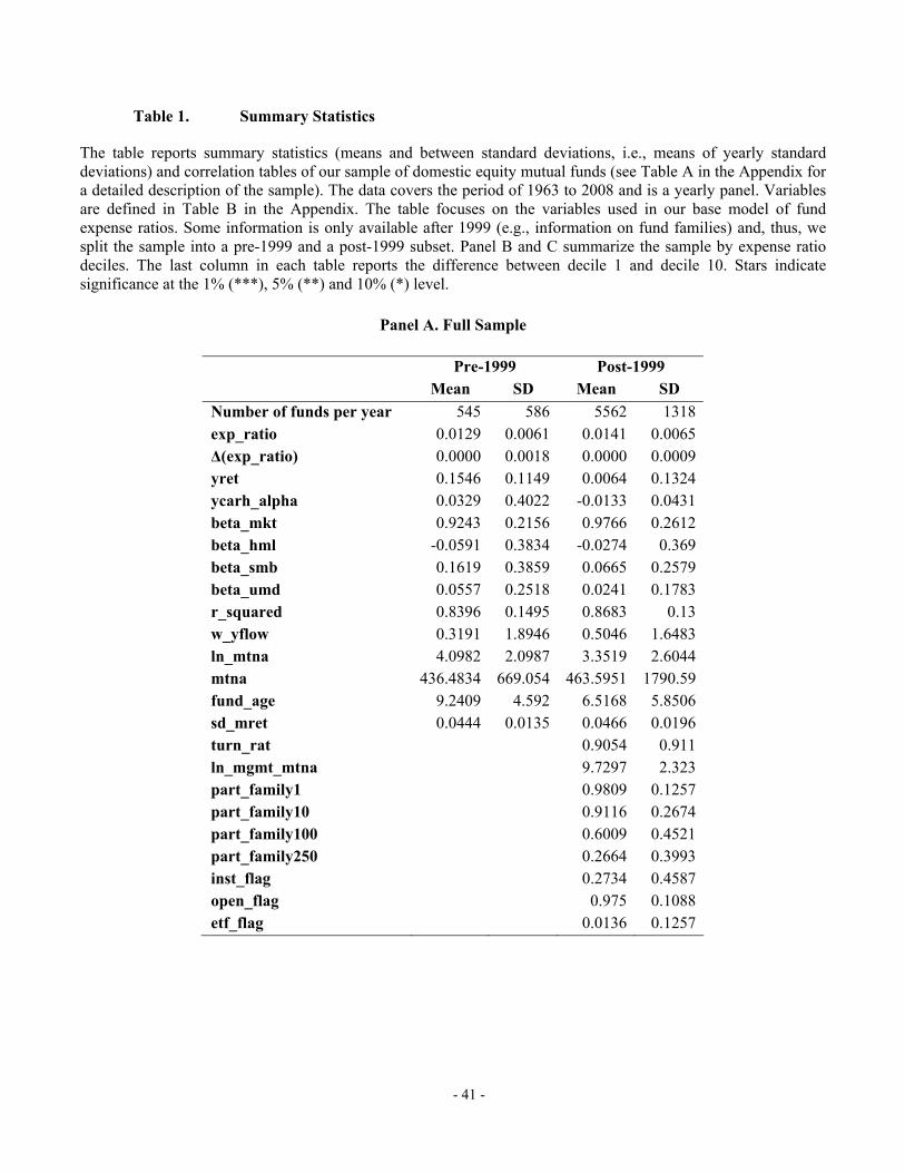
- 41 -

Table 1. Summary Statistics

The table reports summary statistics (means and between standard deviations, i.e., means of yearly standard deviations) and correlation tables of our sample of domestic equity mutual funds (see Table A in the Appendix for a detailed description of the sample). The data covers the period of 1963 to 2008 and is a yearly panel. Variables are defined in Table B in the Appendix. The table focuses on the variables used in our base model of fund expense ratios. Some information is only available after 1999 (e.g., information on fund families) and, thus, we split the sample into a pre-1999 and a post-1999 subset. Panel B and C summarize the sample by expense ratio deciles. The last column in each table reports the difference between decile 1 and decile 10. Stars indicate significance at the 1% (***), 5% (**) and 10% (*) level.

Panel A. Full Sample

Pre-1999 Post-1999 Mean SD Mean SD

Number of funds per year 545 586 5562 1318 exp_ratio 0.0129 0.0061 0.0141 0.0065 Δ(exp_ratio) 0.0000 0.0018 0.0000 0.0009 yret 0.1546 0.1149 0.0064 0.1324 ycarh_alpha 0.0329 0.4022 -0.0133 0.0431 beta_mkt 0.9243 0.2156 0.9766 0.2612 beta_hml -0.0591 0.3834 -0.0274 0.369 beta_smb 0.1619 0.3859 0.0665 0.2579 beta_umd 0.0557 0.2518 0.0241 0.1783 r_squared 0.8396 0.1495 0.8683 0.13 w_yflow 0.3191 1.8946 0.5046 1.6483 ln_mtna 4.0982 2.0987 3.3519 2.6044 mtna 436.4834 669.054 463.5951 1790.59 fund_age 9.2409 4.592 6.5168 5.8506 sd_mret 0.0444 0.0135 0.0466 0.0196 turn_rat 0.9054 0.911 ln_mgmt_mtna 9.7297 2.323 part_family1 0.9809 0.1257 part_family10 0.9116 0.2674 part_family100 0.6009 0.4521 part_family250 0.2664 0.3993 inst_flag 0.2734 0.4587 open_flag 0.975 0.1088 etf_flag 0.0136 0.1257

- 42 -

Panel B. Summary Statistics by Expense Ratio Deciles – Pre-1999 Sample

Decile 1 Decile 3 Decile 5 Decile 7 Decile 10 Decile 1-10

Mean SD Mean SD Mean SD Mean SD Mean SD Diff.

exp_ratio 0.0052 0.0018 0.0089 0.001 0.0111 0.0014 0.0141 0.0022 0.0257 0.0059 -0.021***

Δ(exp_ratio) -0.0006 0.0052 -0.0002 0.0018 -0.0001 0.0021 -0.0003 0.0025 0.0015 0.0057 -0.002***

yret 0.1581 0.112 0.1613 0.1152 0.1518 0.1241 0.1503 0.1332 0.1287 0.1479 0.029***

ycarh_alpha -0.0021 0.0423 -0.0041 0.0547 -0.0055 0.0592 -0.0119 0.0629 -0.0251 0.0711 0.023***

beta_mkt 0.9327 0.2071 0.929 0.1699 0.9274 0.211 0.918 0.2143 0.9274 0.2723 0.005

beta_hml -0.026 0.3245 -0.0461 0.3033 -0.05 0.3711 -0.0419 0.3583 -0.108 0.4576 0.082***

beta_smb -0.0029 0.2884 0.0733 0.2886 0.1579 0.3586 0.2008 0.3685 0.3341 0.511 -0.337***

beta_umd 0.0116 0.1893 0.0395 0.1942 0.0473 0.23 0.0746 0.2324 0.0807 0.3337 -0.069***

r_squared 0.8896 0.1613 0.8698 0.1257 0.8446 0.1448 0.8224 0.1594 0.7632 0.1968 0.126***

w_yflow 0.1908 1.7286 0.2367 1.6338 0.2603 1.409 0.3424 1.3676 0.4338 2.0533 -0.243***

ln_mtna 5.7637 2.2359 4.9996 1.926 4.2314 1.9302 3.6769 1.8869 2.2615 1.7367 3.502***

mtna 1581 4294 581 1870 294 1088 215 671 48 105 1533.5***

mtna_share 0.723% 0.553% 0.237% 0.474% 0.119% 0.314% 0.067% 0.122% 0.025% 0.103% 0.70%***

fund_age 13.2252 9.1036 12.2635 8.9289 10.1815 7.4482 7.5967 5.9195 6.329 4.8624 6.896***

sd_mret 0.0405 0.0171 0.0415 0.0122 0.0436 0.0166 0.0449 0.0154 0.0511 0.0164 -0.011***

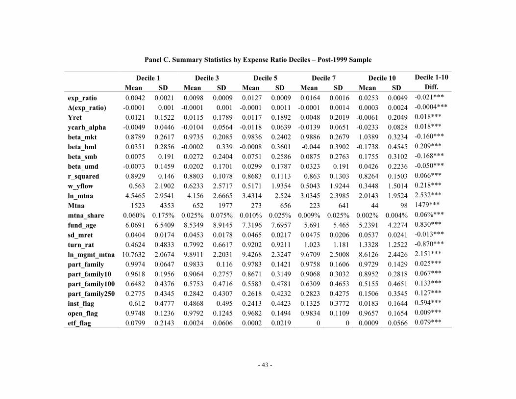
- 43 -

Panel C. Summary Statistics by Expense Ratio Deciles – Post-1999 Sample

Decile 1 Decile 3 Decile 5 Decile 7 Decile 10 Decile 1-10

Mean SD Mean SD Mean SD Mean SD Mean SD Diff.

exp_ratio 0.0042 0.0021 0.0098 0.0009 0.0127 0.0009 0.0164 0.0016 0.0253 0.0049 -0.021***

Δ(exp_ratio) -0.0001 0.001 -0.0001 0.001 -0.0001 0.0011 -0.0001 0.0014 0.0003 0.0024 -0.0004***

Yret 0.0121 0.1522 0.0115 0.1789 0.0117 0.1892 0.0048 0.2019 -0.0061 0.2049 0.018***

ycarh_alpha -0.0049 0.0446 -0.0104 0.0564 -0.0118 0.0639 -0.0139 0.0651 -0.0233 0.0828 0.018***

beta_mkt 0.8789 0.2617 0.9735 0.2085 0.9836 0.2402 0.9886 0.2679 1.0389 0.3234 -0.160***

beta_hml 0.0351 0.2856 -0.0002 0.339 -0.0008 0.3601 -0.044 0.3902 -0.1738 0.4545 0.209***

beta_smb 0.0075 0.191 0.0272 0.2404 0.0751 0.2586 0.0875 0.2763 0.1755 0.3102 -0.168***

beta_umd -0.0073 0.1459 0.0202 0.1701 0.0299 0.1787 0.0323 0.191 0.0426 0.2236 -0.050***

r_squared 0.8929 0.146 0.8803 0.1078 0.8683 0.1113 0.863 0.1303 0.8264 0.1503 0.066***

w_yflow 0.563 2.1902 0.6233 2.5717 0.5171 1.9354 0.5043 1.9244 0.3448 1.5014 0.218***

ln_mtna 4.5465 2.9541 4.156 2.6665 3.4314 2.524 3.0345 2.3985 2.0143 1.9524 2.532***

Mtna 1523 4353 652 1977 273 656 223 641 44 98 1479***

mtna_share 0.060% 0.175% 0.025% 0.075% 0.010% 0.025% 0.009% 0.025% 0.002% 0.004% 0.06%***

fund_age 6.0691 6.5409 8.5349 8.9145 7.3196 7.6957 5.691 5.465 5.2391 4.2274 0.830***

sd_mret 0.0404 0.0174 0.0453 0.0178 0.0465 0.0217 0.0475 0.0206 0.0537 0.0241 -0.013***

turn_rat 0.4624 0.4833 0.7992 0.6617 0.9202 0.9211 1.023 1.181 1.3328 1.2522 -0.870***

ln_mgmt_mtna 10.7632 2.0674 9.8911 2.2031 9.4268 2.3247 9.6709 2.5008 8.6126 2.4426 2.151***

part_family 0.9974 0.0647 0.9833 0.116 0.9783 0.1421 0.9758 0.1606 0.9729 0.1429 0.025***

part_family10 0.9618 0.1956 0.9064 0.2757 0.8671 0.3149 0.9068 0.3032 0.8952 0.2818 0.067***

part_family100 0.6482 0.4376 0.5753 0.4716 0.5583 0.4781 0.6309 0.4653 0.5155 0.4651 0.133***

part_family250 0.2775 0.4345 0.2842 0.4307 0.2618 0.4232 0.2823 0.4275 0.1506 0.3545 0.127***

inst_flag 0.612 0.4777 0.4868 0.495 0.2413 0.4423 0.1325 0.3772 0.0183 0.1644 0.594***

open_flag 0.9748 0.1236 0.9792 0.1245 0.9682 0.1494 0.9834 0.1109 0.9657 0.1654 0.009***

etf_flag 0.0799 0.2143 0.0024 0.0606 0.0002 0.0219 0 0 0.0009 0.0566 0.079***

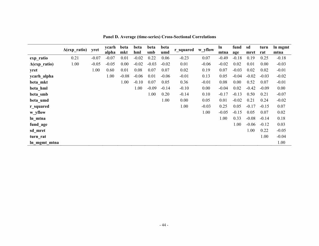
- 44 -

Panel D. Average (time-series) Cross-Sectional Correlations

Δ(exp_ratio) yret ycarhalpha

beta mkt

beta hml

beta smb

beta umd

r_squared w_yflowln mtna

fund age

sd mret

turn rat

ln mgmtmtna

exp_ratio 0.21 -0.07 -0.07 0.01 -0.02 0.22 0.06 -0.23 0.07 -0.49 -0.18 0.19 0.25 -0.18 Δ(exp_ratio) 1.00 -0.05 -0.05 0.00 -0.02 -0.03 -0.02 0.01 -0.06 -0.02 0.02 0.01 0.00 -0.03 yret 1.00 0.60 0.01 0.08 0.07 0.07 0.02 0.19 0.07 -0.03 0.02 0.02 -0.01 ycarh_alpha 1.00 -0.08 -0.06 0.01 -0.06 -0.01 0.13 0.05 -0.04 -0.02 -0.03 -0.02 beta_mkt 1.00 -0.10 0.07 0.05 0.36 -0.01 0.08 0.00 0.52 0.07 -0.01 beta_hml 1.00 -0.09 -0.14 -0.10 0.00 -0.04 0.02 -0.42 -0.09 0.00 beta_smb 1.00 0.20 -0.14 0.10 -0.17 -0.13 0.50 0.21 -0.07 beta_umd 1.00 0.00 0.05 0.01 -0.02 0.21 0.24 -0.02 r_squared 1.00 -0.03 0.25 0.05 -0.17 -0.15 0.07 w_yflow 1.00 -0.05 -0.15 0.05 0.07 0.02 ln_mtna 1.00 0.33 -0.08 -0.14 0.18 fund_age 1.00 -0.06 -0.12 0.03 sd_mret 1.00 0.22 -0.05 turn_rat 1.00 -0.04 ln_mgmt_mtna 1.00

- 45 -

Table 2. Base Case Fund Fee Regressions

The table reports results of Fama-MacBeth regressions, in which we use the yearly expense ratio as dependent variables (see Table A in the Appendix for a detailed description of the sample). The data covers the period of 1963 to 2008 and is a yearly panel. Variables are defined in Table B in the Appendix. All variables are lagged by one year. Some information is only available after 1999 (e.g., information on fund families) and, thus, we split the sample into a pre-1999 and a post-1999 subset. The specifications reported in this table represent the base case specifications. We look at the full sample of mutual funds, the largest, and smallest (funds in the top or bottom quintile of mtna in a given year) funds.

Pre 1999 Post 1999 Full Sample Largest Funds Smallest Funds Full Sample Largest Funds Smallest Funds Coeff. t-value Coeff. t-value Coeff. t-value Coeff. t-value Coeff. t-value Coeff. t-value

Yrett-1 -0.0077 -4.61 -0.0045 -2.19 -0.0129 -1.62 -0.0064 -4.88 -0.0052 -3.61 -0.0112 -6.47beta_mkt t-1 0.0016 1.72 -0.0067 -2.51 0.0032 0.85 -0.0005 -0.72 0.0009 0.87 -0.0005 -0.49beta_hml t-1 0.0007 1.37 0.0036 4.21 -0.0026 -1.22 0.0007 2.50 0.0001 0.16 0.0004 0.56beta_smb t-1 0.0019 3.35 -0.0010 -1.13 0.0014 0.56 -0.0004 -1.73 0.0003 0.79 -0.0009 -1.81beta_umd t-1 0.0009 1.62 0.0025 2.71 0.0027 1.27 0.0001 0.16 0.0010 2.60 -0.0026 -1.34r_squared t-1 -0.0049 -5.26 -0.0060 -1.60 -0.0115 -3.00 -0.0030 -3.83 -0.0034 -4.19 -0.0047 -3.67flow t-1 0.0001 0.18 0.0000 0.04 -0.0014 -1.06 -0.0001 -2.63 -0.0002 -1.55 0.0000 -0.77ln_mtna t-1 -0.0016 -18.64 -0.0006 -8.98 -0.0031 -7.01 -0.0007 -29.24 -0.0008 -11.89 -0.0003 -3.59fund_age t-1 -0.0000 -5.08 -0.0001 -0.90 0.0000 0.11 -0.0001 -9.72 -0.0001 -8.29 0.0003 5.29sd_mret t-1 0.0245 1.34 0.1332 2.46 0.0537 0.56 0.1001 7.04 0.0181 0.70 0.1318 5.51turn_rat t-1 0.0002 3.85 0.0003 3.68 0.0001 1.01ln_mgmt_mtna t-1 -0.0004 -11.06 -0.0008 -11.15 -0.0006 -7.41part_family100 0.0017 8.81 0.0027 10.93 0.0006 2.51inst_flag -0.0063 -44.74 -0.0048 -25.53 -0.0071 -19.75open_flag -0.0001 -0.26 0.0004 1.02 -0.0025 -1.87etf_flag -0.0032 -4.29 -0.0028 -3.68Constant 0.0203 21.59 0.0184 4.33 0.0291 8.26 0.0210 19.16 0.0257 20.30 0.0238 16.87# of years 34 34 34 10 10 10 # of obs. 12108 3018 1670 33323 8592 3994 Avg. R-Squared 44.3% 49.3% 54.7% 44.1% 39.0% 56.2%

- 46 -

Table 3. Residual Fee Spreads Including Robustness Tests

The table summarizes (time-series) mean spreads between percentiles of the residual fee distribution for our sample of mutual funds (see Table A in the Appendix for a detailed description of the sample). The residual fee is defined as the regression residual of the corresponding (full sample/largest funds/smallest funds) fund fee regression model as specified in Table 2. The first row of each panel contains the residual fee spreads from these specific models. The other rows represent robustness tests and provide residual fee spreads for models in which we vary the fund characteristics used to estimate fee residuals. The data covers the period of 1963 to 2008 and is a yearly panel. The variables are defined in Table B of the Appendix. Rows 2 to 5 report residual fee spreads if we vary fund performance measures. Rows 6 to 9 report results of specifications that use gross (i.e., before-fee) rather than net performance measures in the regressions to explain expense ratios. Row 10 reports the results for a specification that includes fund style fixed effects. Rows 11 to 12 report results that use performance measures derived from expanding rather than rolling windows (in this case, we also use beta estimates from expanding windows). Rows 13 to 15 report mean fee spreads for specifications in which we reduce the estimation noise in four-factor alphas and betas. In Row 13 we set the estimated alpha and betas to 0 if the corresponding t-statistic is below 3 in absolute terms and in rows 14 and 15 we use full sample estimates of these asset pricing parameters (i.e., for each fund we estimate these parameters using all available data and then we use the same parameters each year to explain expense ratios).

- 47 -

Panel A. Full Sample Mean Spread (bps)

25th to 75th Percentile

Mean Spread (bps) 10th to 90th Percentile

Mean Spread (bps)

1st to 99th Percentile

1 Yearly return (Yrett-1) 44 89 234 2 Yearly return (Yrett-1)

+ persistence dummy 44 88 234

3 Four-factor alpha (Yalphat-1) + persistence dummy

44 88 231

4 T-statistic of four-factor Alpha (TStat-Alphat-1) + persistence dummy

43 87 234

5 Carhart alpha (Ycarh_alphat-1) + persistence dummy

44 88 234

6 Before-expense yearly return 44 88 230 7 Before-expense yearly return

+ before-expense persistence dummy

44 88 230

8 Before-expense four-factor alpha + before-expense persistence dummy

44 88 228

9 Before-expense Carhart performance + before-expense persistence dummy

44 87 230

10 Style fixed effects +yearly return (Yrett-1)

42 87 215

11 Expanding window + four-factor alpha

43 86 239

12 Expanding window + t-statistic of four-factor Alpha

44 86 241

13 Filtered alphas/betas + four-factor alpha

43 88 236

14 Full Sample + four-factor alpha

43 86 227

15 Full sample + t-statistic of alpha

44 87 233

- 48 -

Panel B. Bottom Size Quintile of Funds

Mean Spread (bps)25th to 75th Percentile

Mean Spread (bps) 10th to 90th Percentile

Mean Spread (bps)1st to 99th Percentile

1 Yearly return (Yrett-1) 65 137 288 2 Yearly return (Yrett-1)

+ persistence dummy 65 136 284

3 Four-factor alpha (Yalphat-1) + persistence dummy

62 131 279

4 T-statistic of four-factor Alpha (TStat-Alphat-1) + persistence dummy

65 135 280

5 Carhart alpha (Ycarh_alphat-1) + persistence dummy

65 134 282

6 Before-expense yearly return 65 133 282 7 Before-expense yearly return

+ before-expense persistence dummy65 130 279

8 Before-expense four-factor alpha + before-expense persistence dummy

66 129 275

9 Before-expense Carhart performance + before-expense persistence dummy

65 129 279

10 Style fixed effects +yearly return (Yrett-1)

48 101 220

11 Expanding window + four-factor alpha

64 126 284

12 Expanding window + t-statistic of four-factor Alpha

64 130 288

13 Filtered alphas/betas + four-factor alpha

66 136 302

14 Full Sample + four-factor alpha

63 125 279

15 Full sample + t-statistic of alpha

65 131 287

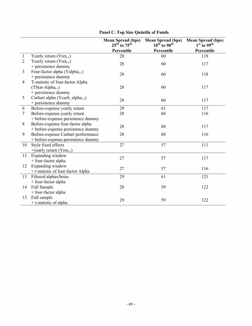
- 49 -

Panel C. Top Size Quintile of Funds

Mean Spread (bps)25th to 75th Percentile

Mean Spread (bps) 10th to 90th Percentile

Mean Spread (bps)1st to 99th Percentile

1 Yearly return (Yrett-1) 28 60 118 2 Yearly return (Yrett-1)

+ persistence dummy 28 60 117

3 Four-factor alpha (Yalphat-1) + persistence dummy

28 60 118

4 T-statistic of four-factor Alpha (TStat-Alphat-1) + persistence dummy

28 60 117

5 Carhart alpha (Ycarh_alphat-1) + persistence dummy

28 60 117

6 Before-expense yearly return 29 61 117 7 Before-expense yearly return

+ before-expense persistence dummy 28 60 116

8 Before-expense four-factor alpha + before-expense persistence dummy

28 60 117

9 Before-expense Carhart performance + before-expense persistence dummy

28 60 116

10 Style fixed effects +yearly return (Yrett-1)

27 57 111

11 Expanding window + four-factor alpha

27 57 117

12 Expanding window + t-statistic of four-factor Alpha

27 57 116

13 Filtered alphas/betas + four-factor alpha

29 61 121

14 Full Sample + four-factor alpha

28 59 122

15 Full sample + t-statistic of alpha

29 59 122

- 50 -

Table 4. Trading Strategy

The table summarizes the cumulative (i.e., compounded) Carhart alphas of a strategy that buys funds in the bottom decile according to reported expense ratios (residual expense ratios), and shorts funds in the top deciles according to reported expense ratios (residual expense ratios). Funds are equally-weighed within portfolios. The table also reports the compounded spread between the average reported expense ratio (residual expense ratio) of funds in the top and the bottom decile. The residual fee is defined as the regression residual of Spec. 1 (pre-1999) and Spec. 4 (post-1999) as specified in Panel A of Table 2. Our sample consists of domestic equity mutual funds (see Table A in the Appendix for a detailed description of the sample). The data covers the period of 1963 to 2008 and is a yearly panel. Variables are defined in Table B in the Appendix.

Reported Expense Ratio Residual Expense Ratio

Year α Fee

Spread Year α

Fee Spread

Year α Fee

SpreadYear α

Fee Spread

1963 0.2% 1.5% 1986 30.0% 43.9% 1986 2.1% 28.1% 1964 3.7% 2.6% 1987 31.5% 46.1% 1987 5.9% 29.8% 1965 -0.6% 3.8% 1988 31.9% 48.6% 1988 8.2% 31.5% 1966 1.1% 5.1% 1989 32.3% 51.0% 1966 1.0% 0.9% 1989 8.6% 33.3% 1967 0.1% 6.7% 1990 32.8% 53.3% 1967 -10.7% 2.2% 1990 9.5% 35.2% 1968 -3.3% 7.8% 1991 34.0% 55.5% 1968 -8.9% 2.9% 1991 8.2% 37.0% 1969 6.6% 9.7% 1992 35.4% 57.7% 1969 -6.6% 3.9% 1992 5.9% 38.9% 1970 7.2% 11.5% 1993 41.5% 59.8% 1970 -5.6% 5.2% 1993 9.1% 40.5% 1971 9.4% 14.0% 1994 46.1% 61.8% 1971 -10.7% 6.9% 1994 11.7% 42.2% 1972 2.3% 15.6% 1995 48.6% 63.9% 1972 -9.9% 7.9% 1995 14.9% 43.8% 1973 1.5% 17.8% 1996 54.2% 65.8% 1973 -4.6% 9.6% 1996 16.3% 45.5% 1974 0.9% 19.9% 1997 52.4% 67.8% 1974 -4.4% 11.0% 1997 19.3% 47.1% 1975 0.5% 22.1% 1998 48.1% 69.7% 1975 -2.4% 12.6% 1998 20.0% 48.7% 1976 5.1% 24.4% 1999 46.7% 71.6% 1976 -1.8% 14.3% 1999 21.5% 50.0% 1977 9.9% 26.5% 2000 52.4% 73.6% 1977 -1.7% 15.6% 2000 23.6% 51.5% 1978 10.1% 28.5% 2001 56.3% 75.7% 1978 -4.2% 17.0% 2001 27.1% 53.0% 1979 11.1% 30.4% 2002 58.5% 78.0% 1979 -5.7% 18.4% 2002 28.2% 54.5% 1980 14.3% 32.5% 2003 61.9% 80.2% 1980 -2.6% 20.0% 2003 30.1% 56.2% 1981 28.2% 34.6% 2004 60.9% 82.3% 1981 1.7% 21.4% 2004 31.5% 57.8% 1982 31.3% 36.6% 2005 63.5% 84.4% 1982 0.6% 22.8% 2005 32.9% 59.3% 1983 33.2% 38.5% 2006 64.5% 86.4% 1983 2.3% 24.1% 2006 33.5% 60.8% 1984 31.1% 40.2% 2007 67.1% 88.5% 1984 4.2% 25.3% 2007 32.2% 62.3% 1985 29.1% 42.1% 2008 67.1% 90.5% 1985 3.4% 26.8% 2008 32.2% 63.8%

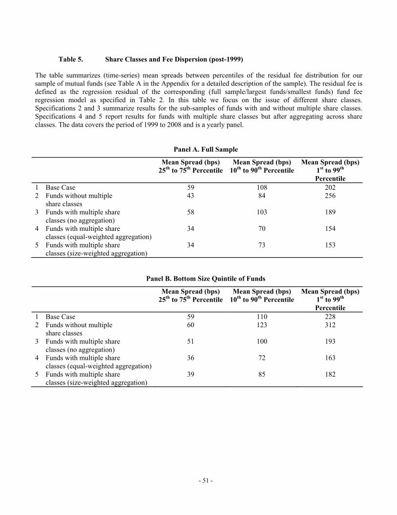
- 51 -

Table 5. Share Classes and Fee Dispersion (post-1999)

The table summarizes (time-series) mean spreads between percentiles of the residual fee distribution for our sample of mutual funds (see Table A in the Appendix for a detailed description of the sample). The residual fee is defined as the regression residual of the corresponding (full sample/largest funds/smallest funds) fund fee regression model as specified in Table 2. In this table we focus on the issue of different share classes. Specifications 2 and 3 summarize results for the sub-samples of funds with and without multiple share classes. Specifications 4 and 5 report results for funds with multiple share classes but after aggregating across share classes. The data covers the period of 1999 to 2008 and is a yearly panel.

Panel A. Full Sample

Mean Spread (bps) 25th to 75th Percentile

Mean Spread (bps) 10th to 90th Percentile

Mean Spread (bps)1st to 99th Percentile

1 Base Case 59 108 202 2 Funds without multiple

share classes 43 84 256

3 Funds with multiple share classes (no aggregation)

58 103 189

4 Funds with multiple share classes (equal-weighted aggregation)

34 70 154

5 Funds with multiple share classes (size-weighted aggregation)

34 73 153

Panel B. Bottom Size Quintile of Funds

Mean Spread (bps) 25th to 75th Percentile

Mean Spread (bps) 10th to 90th Percentile

Mean Spread (bps)1st to 99th Percentile

1 Base Case 59 110 228 2 Funds without multiple

share classes 60 123 312

3 Funds with multiple share classes (no aggregation)

51 100 193

4 Funds with multiple share classes (equal-weighted aggregation)

36 72 163

5 Funds with multiple share classes (size-weighted aggregation)

39 85 182

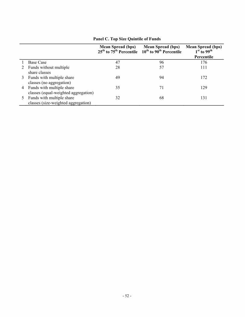
- 52 -

Panel C. Top Size Quintile of Funds

Mean Spread (bps) 25th to 75th Percentile

Mean Spread (bps) 10th to 90th Percentile

Mean Spread (bps)1st to 99th Percentile

1 Base Case 47 96 176 2 Funds without multiple

share classes 28 57 111

3 Funds with multiple share classes (no aggregation)

49 94 172

4 Funds with multiple share classes (equal-weighted aggregation)

35 71 129

5 Funds with multiple share classes (size-weighted aggregation)

32 68 131

- 53 -

Table 6. Testing Explanations of Residual Fee Spreads

The table shows results related to variables that capture different hypotheses that we evaluate in order to explain the dispersion in mutual fund fees. Panel A reports means and standard deviations of our proxies by raw expense ratio deciles. The last column reports the difference between decile 1 and decile 10. Stars indicate significance at the 1% (***), 5% (**) and 10% (*) level. Panel B and C report coefficients of these variables if they are added individually or all together to the base case specifications described in Table 2. For brevity we focus on the results for the full sample of funds. Panel D, reports mean residual fee spreads for groups of funds after including these proxies individually or jointly in the fee regressions. Variables are defined in Table B in the Appendix.

Panel A. Summary Statistics of Proxies by Raw Expense Ratio Deciles

Decile 1 Decile 3 Decile 5 Decile 7 Decile 10 Decile 1-10 Mean SD Mean SD Mean SD Mean SD Mean SD Diff.

rand_feechgs 0.158 0.126 0.175 0.142 0.161 0.134 0.138 0.126 0.100 0.097 0.058***

compALL_funds 9.104 10.996 8.99 10.65 10.53 13.57 10.22 13.41 11.69 14.87 -2.58***

compALL_fees 0.011 0.003 0.012 0.002 0.013 0.003 0.014 0.003 0.017 0.003 -0.006*** flow_auto 0.019 0.275 0.027 0.257 0.061 0.287 0.124 0.341 0.182 0.362 -0.163*** P

re-1

999

“Pension Plan” 0.019 0.162 0.013 0.154 0.029 0.203 0.078 0.301 0.087 0.327 -0.068***

rand_feechgs 0.068 0.089 0.128 0.129 0.128 0.128 0.113 0.121 0.119 0.116 -0.051***

compALL_funds 63.12 49.46 54.16 40.75 53.49 42.59 54.51 41.46 56.16 40.72 6.96***

compALL_fees 0.012 0.002 0.014 0.002 0.014 0.002 0.014 0.002 0.016 0.003 -0.004***

flow_perf 0.140 3.347 0.004 1.905 0.165 2.209 0.080 2.087 0.187 1.920 -0.046*** flow_auto 0.183 0.310 0.163 0.298 0.231 0.316 0.341 0.349 0.364 0.369 -0.181*** “Pension Plan” 0.048 0.226 0.041 0.207 0.077 0.268 0.161 0.338 0.184 0.375 -0.136***

Pos

t-19

99

“Easy-In Hard-Out” 0.000 0.000 0.000 0.000 0.000 0.000 0.006 0.053 0.033 0.175 -0.033***

- 54 -

Panel B. Coefficients in Fee Regressions (Pre-1999)

Controlling for… Randomization Competition Captivity All Coeff. t-value Coeff. t-value Coeff. t-value Coeff. t-value

rand_feechgs 0.0016 2.97 0.0016 2.85compALL_funds -0.0001 -3.11 -0.0001 -3.24compALL_fees 0.5126 10.63 0.4970 11.99flow_auto 0.0016 2.79 0.0007 1.05“Pension Plan” 0.0003 2.14 0.0002 2.22Family Fixed Effects No No No No Other Controls Like Table 2 Like Table 2 Like Table 2 Like Table 2 # of years 34 34 34 34 # of obs. 12108 10416 12108 10416 Avg. R-Squared 44.7% 51.3% 45.1% 52.5

Panel C. Coefficients in Fee Regressions (Post-1999)

Controlling for… Randomization Competition Flow-Perf. Sens. Captivity 1 Captivity 2 All Coeff. t-value Coeff. t-value Coeff. t-value Coeff. t-value Coeff. t-value Coeff. t-value

rand_feechgs 0.0038 8.84 0.0031 9.59compALL_funds -0.0000 -2.21 -0.0000 -4.50compALL_fees 0.5259 24.24 0.4650 22.24flow_perf 0.0002 2.25 0.0001 1.76flow_auto 0.0035 17.78 0.0031 15.24“Pension Plan” 0.0012 11.12 0.0013 12.87“Easy-In Hard-Out” 0.0021 3.64Family Fixed Effects No No No No No Yes Other Controls Like Table 2 Like Table 2 Like Table 2 Like Table 2 Like Table 2 Like Table 2 # of years 10 10 10 10 10 10 # of obs. 33323 33257 33315 33323 15745 33249 Avg. R-Squared 44.7% 46.9% 44.2% 48.8% 36.0% 53.5%

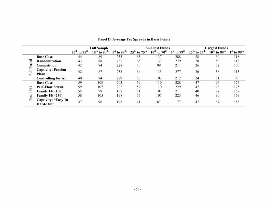
- 55 -

Panel D. Average Fee Spreads in Basis Points

Full Sample Smallest Funds Largest Funds 25th to 75th 10th to 90th 1st to 99th 25th to 75th 10th to 90th 1st to 99th 25th to 75th 10th to 90th 1st to 99th

Base Case 44 89 235 65 137 288 28 60 118 Randomization 43 88 235 65 137 279 28 59 113 Competition 42 84 228 50 99 211 26 52 100 Captivity: Pension

Plans 42 87 233 64 135 277 26 58 115

Ful

l Per

iod

Controlling for All 40 84 229 50 102 212 24 51 98 Base Case 59 108 202 59 110 228 47 96 176 Perf-Flow Sensit. 59 107 202 59 110 229 47 96 175 Family FE (100) 55 99 187 51 101 211 40 77 157 Family FE (250) 58 105 198 57 107 223 46 90 169 P

ost-

1999

Captivity: “Easy-In Hard-Out”

47 96 198 41 87 177 47 87 183

- 56 -

Table 7. Transition Probabilities between Fee Quintiles

The table summarizes 1-year and 2-year transition probabilities between fee quintiles for our sample of mutual funds (see Table A in the Appendix for a detailed description of the sample). In Panel A and C we look at expense ratios. In Panel B and D, the residual fee is defined as the regression residual of Spec. 1 (pre-1999) and Spec. 4 (post-1999) as specified in Panel A of Table 2. In Panels A and B, we determine the quintile thresholds using all funds within one year. In Panels C and D, we determine the quintile thresholds using only “old” funds (i.e., funds that were in the sample in the previous year) within one year. The data covers the period of 1963 to 2008 and is a yearly panel. Variables are defined in Table B in the Appendix.

Panel A. Expense Ratios (All Funds)

Low Fees (t-12) 2 (t-12) 3 (t-12) 4 (t-12) High Fees (t-12) Low Fees 87.0% 11.0% 0.7% 0.7% 0.6% 2 8.4% 72.7% 16.5% 1.7% 0.7% 3 1.1% 11.3% 68.7% 17.4% 1.5% 4 0.5% 1.6% 11.8% 69.8% 16.3% High Fees 0.7% 0.5% 1.6% 12.4% 84.7% Low Fees (t-24) 2 (t-24) 3 (t-24) 4 (t-24) High Fees (t-24) Low Fees 80.9% 16.1% 1.4% 0.8% 0.7% 2 10.7% 61.4% 24.1% 2.7% 1.0% 3 1.9% 14.1% 57.3% 24.0% 2.7% 4 0.7% 2.5% 14.0% 59.5% 23.3% High Fees 0.8% 0.7% 1.8% 15.6% 81.0%

Panel B. Residual Fees (All Funds)

Low Fees (t-12) 2 (t-12) 3 (t-12) 4 (t-12) High Fees (t-12) Low Fees 70.1% 19.4% 5.9% 2.5% 2.0% 2 20.6% 46.1% 22.5% 7.7% 3.0% 3 6.6% 21.8% 43.2% 21.9% 6.5% 4 3.4% 7.9% 21.3% 48.8% 18.5% High Fees 2.4% 4.1% 6.1% 17.7% 69.7% Low Fees (t-24) 2 (t-24) 3 (t-24) 4 (t-24) High Fees (t-24) Low Fees 62.2% 22.5% 7.5% 4.5% 3.2% 2 23.9% 38.5% 23.8% 9.1% 4.6% 3 9.1% 22.9% 36.7% 23.2% 8.1% 4 4.7% 11.0% 21.5% 41.5% 21.4% High Fees 3.2% 4.7% 8.7% 20.9% 62.5%

- 57 -

Panel C. Expense Ratios (Old Funds Only)

Low Fees (t-12) 2 (t-12) 3 (t-12) 4 (t-12) High Fees (t-12) Low Fees 86.8% 11.3% 0.7% 0.4% 0.8% 2 8.3% 71.6% 17.5% 2.1% 0.5% 3 1.0% 11.1% 67.5% 18.4% 1.9% 4 0.5% 1.3% 12.5% 69.9% 15.8% High Fees 0.7% 0.4% 1.5% 10.4% 87.0% Low Fees (t-24) 2 (t-24) 3 (t-24) 4 (t-24) High Fees (t-24) Low Fees 80.3% 16.5% 1.5% 0.7% 0.9% 2 10.8% 60.1% 25.0% 3.0% 1.1% 3 2.0% 13.3% 56.9% 25.2% 2.7% 4 0.6% 2.4% 13.9% 59.9% 23.2% High Fees 0.7% 0.5% 1.7% 12.9% 84.1%

Panel D. Residual Fees (Old Funds Only)

Low Fees (t-12) 2 (t-12) 3 (t-12) 4 (t-12) High Fees (t-12) Low Fees 70.1% 19.2% 6.2% 2.3% 2.1% 2 21.5% 44.9% 22.7% 7.7% 3.1% 3 7.5% 22.0% 41.7% 22.2% 6.7% 4 3.8% 7.5% 20.9% 47.8% 20.1% High Fees 2.7% 4.1% 5.9% 17.9% 69.5% Low Fees (t-24) 2 (t-24) 3 (t-24) 4 (t-24) High Fees (t-24) Low Fees 63.0% 21.4% 8.1% 4.2% 3.4% 2 25.0% 37.9% 22.6% 9.7% 4.9% 3 10.1% 22.3% 36.2% 23.0% 8.4% 4 4.8% 11.1% 21.0% 40.4% 22.8% High Fees 3.5% 4.9% 8.6% 20.4% 62.6%

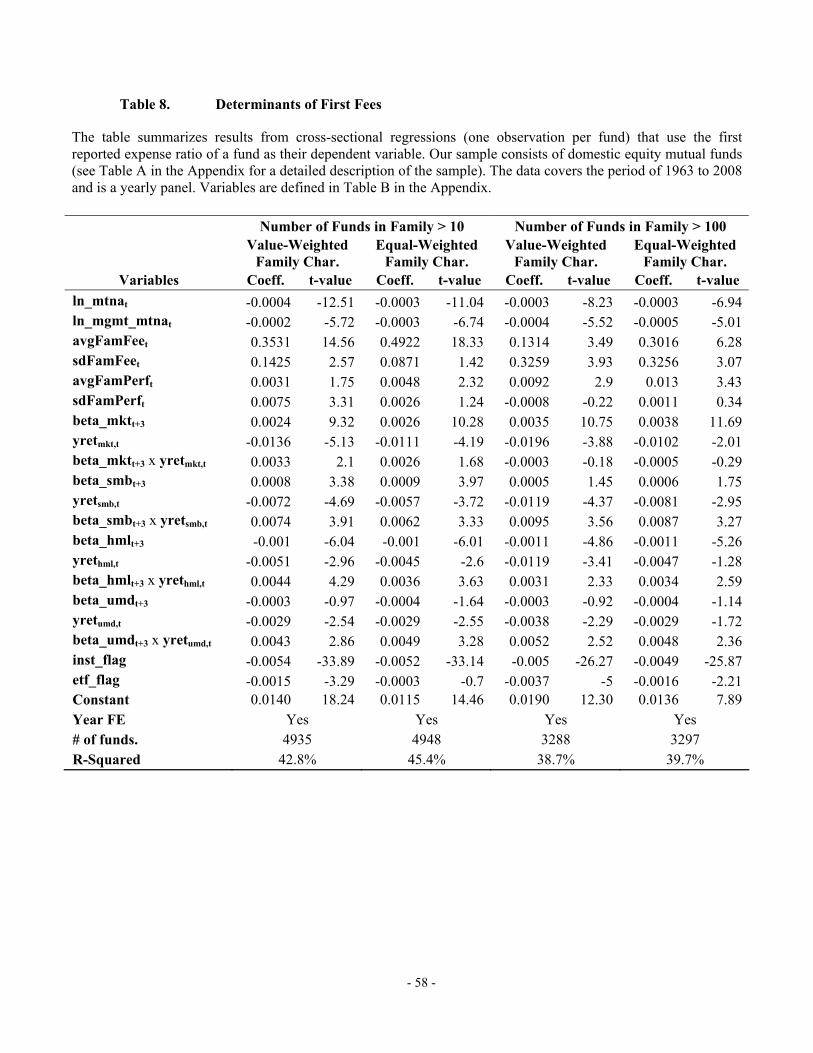
- 58 -

Table 8. Determinants of First Fees

The table summarizes results from cross-sectional regressions (one observation per fund) that use the first reported expense ratio of a fund as their dependent variable. Our sample consists of domestic equity mutual funds (see Table A in the Appendix for a detailed description of the sample). The data covers the period of 1963 to 2008 and is a yearly panel. Variables are defined in Table B in the Appendix.

Number of Funds in Family > 10 Number of Funds in Family > 100

Value-Weighted

Family Char. Equal-Weighted

Family Char. Value-Weighted

Family Char. Equal-Weighted

Family Char. Variables Coeff. t-value Coeff. t-value Coeff. t-value Coeff. t-value

ln_mtnat -0.0004 -12.51 -0.0003 -11.04 -0.0003 -8.23 -0.0003 -6.94ln_mgmt_mtnat -0.0002 -5.72 -0.0003 -6.74 -0.0004 -5.52 -0.0005 -5.01avgFamFeet 0.3531 14.56 0.4922 18.33 0.1314 3.49 0.3016 6.28sdFamFeet 0.1425 2.57 0.0871 1.42 0.3259 3.93 0.3256 3.07avgFamPerft 0.0031 1.75 0.0048 2.32 0.0092 2.9 0.013 3.43sdFamPerft 0.0075 3.31 0.0026 1.24 -0.0008 -0.22 0.0011 0.34beta_mktt+3 0.0024 9.32 0.0026 10.28 0.0035 10.75 0.0038 11.69yretmkt,t -0.0136 -5.13 -0.0111 -4.19 -0.0196 -3.88 -0.0102 -2.01beta_mktt+3 x yretmkt,t 0.0033 2.1 0.0026 1.68 -0.0003 -0.18 -0.0005 -0.29beta_smbt+3 0.0008 3.38 0.0009 3.97 0.0005 1.45 0.0006 1.75yretsmb,t -0.0072 -4.69 -0.0057 -3.72 -0.0119 -4.37 -0.0081 -2.95beta_smbt+3 x yretsmb,t 0.0074 3.91 0.0062 3.33 0.0095 3.56 0.0087 3.27beta_hmlt+3 -0.001 -6.04 -0.001 -6.01 -0.0011 -4.86 -0.0011 -5.26yrethml,t -0.0051 -2.96 -0.0045 -2.6 -0.0119 -3.41 -0.0047 -1.28beta_hmlt+3 x yrethml,t 0.0044 4.29 0.0036 3.63 0.0031 2.33 0.0034 2.59beta_umdt+3 -0.0003 -0.97 -0.0004 -1.64 -0.0003 -0.92 -0.0004 -1.14yretumd,t -0.0029 -2.54 -0.0029 -2.55 -0.0038 -2.29 -0.0029 -1.72beta_umdt+3 x yretumd,t 0.0043 2.86 0.0049 3.28 0.0052 2.52 0.0048 2.36inst_flag -0.0054 -33.89 -0.0052 -33.14 -0.005 -26.27 -0.0049 -25.87etf_flag -0.0015 -3.29 -0.0003 -0.7 -0.0037 -5 -0.0016 -2.21Constant 0.0140 18.24 0.0115 14.46 0.0190 12.30 0.0136 7.89Year FE Yes Yes Yes Yes # of funds. 4935 4948 3288 3297 R-Squared 42.8% 45.4% 38.7% 39.7%

- 59 -

Table 9. Determinants of Fee Changes

The table reports results of Fama-MacBeth regressions using the yearly changes in expense ratios as dependent variables (see Table A in the Appendix for a detailed description of the sample). The data covers the period of 1963 to 2008 and is a yearly panel. Variables are defined in Table B in the Appendix. Δ indicates that we calculate simple changes of our base variables. Variables with subscripts t-1 are lagged by one year. Some information is only available after 1999 (e.g., information on fund families) and, thus, we split the sample into a pre-1999 and a post-1999 subset. In the pre-1999 case we only report results for our full sample because sample sizes become very small if we focus on largest and smallest funds.

Pre 1999 Post 1999 Full Sample Full Sample Largest Funds Smallest Funds Coeff. t-value Coeff. t-value Coeff. t-value Coeff. t-value

Yrett-1 -0.0028 -0.85 -0.0013 -5.43 -0.0012 -5.65 -0.0007 -1.27Δbeta_mkt 0.0025 0.30 0.0000 -0.02 0.0001 0.69 0.0016 1.60Δbeta_hml -0.0013 -0.60 -0.0005 -1.06 -0.0002 -0.76 -0.0023 -1.03Δbeta_smb -0.0034 -2.27 0.0010 1.85 0.0003 1.41 0.0033 1.03Δbeta_umd 0.0014 0.28 0.0011 1.53 -0.0005 -1.16 0.0014 0.43Δr_squared -0.0028 -0.44 0.0001 0.13 -0.0002 -0.91 0.0013 0.78CompNew_Funds 0.0014 1.25 0.0000 0.24 0.0000 -0.88 0.0000 0.77CompNew_Fees -0.1088 -1.60 0.0025 1.00 0.0001 0.05 0.0192 1.76flow t-1 0.0007 1.03 0.0000 -1.17 0.0000 -2.07 0.0000 0.61Δln_mtna -0.0006 -0.83 -0.0002 -1.34 -0.0001 -2.92 0.0000 -0.09fund_age -0.0001 -1.00 0.0000 3.45 0.0000 2.21 0.0000 -0.63Δsd_mret 0.0771 0.97 0.0056 0.92 0.0003 0.06 0.0233 0.55Δturn_rat 0.0002 1.22 0.0000 0.57 0.0000 -0.18Δln_mgmt_mtna 0.0000 -0.50 -0.0001 -2.79 -0.0003 -2.57part_family100 0.0000 -0.93 0.0000 -0.52 0.0000 0.08inst_flag 0.0001 1.60 0.0001 1.00 0.0001 0.30open_flag 0.0002 3.44 0.0001 0.85 0.0007 1.40etf_flag 0.0000 0.31 0.0000 0.99 0.0000 0.00Constant 0.0026 1.60 -0.0002 -2.51 -0.0001 -0.72 -0.0007 -2.10# of years 18 10 10 10 # of obs. 4506 21124 5499 2522 Avg. R-Squared 29.0% 15.5% 22.2% 15.6%

60

Table 10. Performance-Flow Sensitivity

The table shows the means, standard deviations and medians of flows and expense ratio changes of groups of funds. All statistics are calculated from pooled data. We group funds by performance: low (high) performance funds are funds in the bottom (top) decile of past year’s returns. We also split funds by different measures of fees into “cheap” (below median) and “expensive” (above median) funds. Performance deciles and expense medians are calculated separately for each year.

First Expense Ratio Expense Ratio Residual Fee

Below Median

Above Median

Below Median

Above Median

Below Median

Above Median

Mean Flows 3.6% -1.3% 4.7% -2.1% 7.5% -7.3%

SD of Flows 113.1% 115.6% 128.4% 106.0% 130.1% 94.7% Median Flows

-11.1% -15.4% -11.2% -15.3% -11.1% -16.8%

Mean Fee Changes

3 bps 3 bps -1 bps 5 bps 0 bps 7 bps

SD of Fee Changes

20 bps 28 bps 13 bps 30 bps 17 bps 32 bps

Median Fee Changes

0 bps 0 bps 0 bps 0 bps 0 bps 1 bps

Low

Funds 1434 2692 1507 2619 2153 1973

Mean 79.4% 65.3% 72.4% 69.6% 86.2% 56.9%

SD 258.5% 188.9% 235.1% 203.7% 272.4% 154.6%

Median 14.0% 15.4% 15.3% 14.3% 15.9% 14.2% Mean Fee Changes

-2 bps -6 bps -3 bps -5 bps -5 bps -4 bps

SD of Fee Changes

11 bps 23 bps 11 bps 24 bps 16 bps 22 bps

Median Fee Changes

0 bps -2 bps -1 bps -2 bps -1 bps -1 bps

Yea

rly

Ret

urn t

-1

High

Funds 1638 2449 1991 2096 1960 2127

61

Figure 1. Fund Fee Dispersion

The figure shows the fee dispersion of expense ratios (left column) and residual expense ratios (right column) across funds and over time. The graphs show the ranges between the 25th and 75th (darkest grey), 10th and 90th (medium dark grey) and 1st and 99th percentile (light grey) points of the distributions. Graphs in the top row also plot the aggregate TNA of all funds in the graph in Billions of USD (connected, dark line). In rows 2 and 3 we include a line (connected, dark line) that represents the fraction of aggregate TNA represented by funds in the bottom size quintile (row 2) and the top size quintile (row 3) of our sample. The residual fee is defined as the regression residual of the fee models specified in Table 2. Our sample consists of domestic equity mutual funds (see Table A in the Appendix for a detailed description of the sample). The data covers the period of 1963 to 2008 and is a yearly panel. Variables are defined in Table B in the Appendix.

Reported Expense Ratios Residual Expense Ratio

Fu

ll S

amp

le

Bot

tom

Qu

inti

le (

Siz

e) F

un

ds

Top

Qu

inti

le (

Siz

e) F

un

ds

62

Figure 2. Fund Fee Dispersion Within and Outside of Fund Families

The figure shows the fee dispersion of expense ratios (left column) and residual expense ratios (right column) across funds that are part of a fund family (top row) and funds that are not (bottom row). The graphs show the ranges between the 25th and 75th (darkest grey), 10th and 90th (medium dark grey) and 1st and 99th percentile (light grey) points of the distributions.. In addition, all graphs include the mean expense ratios or the mean residual expense ratios (black dots). For these plots management companies with more than 100 funds are defined as fund families. The residual fee is defined as the regression residual of the full sample fee model in Table 2. Our sample consists of domestic equity mutual funds (see Table A in the Appendix for a detailed description of the sample). The data in this analysis covers the period of 1999 to 2008 and is a yearly panel. Variables are defined in Table B in the Appendix.

Reported Expense Ratios Residual Expense Ratio

Wit

hin

Fam

ily

Ou

tsid

e F

amil

y

63

Figure 3. Fund Fee Dispersion of Institutional and Retail Funds

The figure shows the fee dispersion of expense ratios (left column) and residual expense ratios (right column) across funds that are institutional funds (top row) and funds that are retail funds (bottom row). The graphs show the ranges between the 25th and 75th (darkest grey), 10th and 90th (medium dark grey) and an1st and 99th percentile (light grey) points of the distributions.. In addition, all graphs include the mean expense ratios or the mean residual expense ratios (black dots). The residual fee is defined as the regression residual of the full sample fee model in Table 2. Our sample consists of domestic equity mutual funds (see Table A in the Appendix for a detailed description of the sample). The data in this analysis covers the period of 1999 to 2008 and is a yearly panel. Variables are defined in Table B in the Appendix.

Reported Expense Ratios Residual Expense Ratio

Inst

itu

tion

al F

un

ds

Ret

ail F

un

ds

64

Figure 4. Evaluation of Trading Strategy

The figure summarizes the cumulative Carhart alpha (the solid line with markers) of a strategy that buys funds, which are in the bottom decile according to reported expense ratios (residual expense ratios), and shorts funds, which are in the top deciles according to reported expense ratios (residual expense ratios). The table also reports the cumulative spread between the average reported expense ratio (residual expense ratio) of funds in the top and the bottom decile (the dashed line). The residual fee is defined as the regression residual of Spec. 1 (pre-1999) and Spec. 4 (post-1999) as specified in Panel A of Table 2. Our sample consists of domestic equity mutual funds (see Table A in the Appendix for a detailed description of the sample). The data covers the period of 1963 to 2008 and is a yearly panel. Variables are defined in Table B in the Appendix.

Panel A. Portfolio selection based on reported expense ratios

Panel B. Portfolio selection based on residual fees