VINTERSJÖFARTSFORSKNING - Trafi.fi · nent deformation and safety margin of shell ... much through...
42
STYRELSEN FÖR VINTERSJÖFARTSFORSKNING WINTER NAVIGATION RESEARCH BOARD Research Report No 99 Mihkel Kõrgesaar and Pentti Kujala VALIDATION OF THE PRELIMINARY ASSESMENT REGARDING THE OPERATIONAL RESTRICTIONS OF SHIPS ICE-STRENGHTENED IN ACCORDANCE WITH THE FINNISH-SWEDISH ICE CLASSES WHEN SAILING IN ICE CONDITIONS IN POLAR WATERS Finnish Transport Safety Agency Swedish Maritime Administration Finnish Transport Agency Swedish Transport Agency Finland Sweden
Transcript of VINTERSJÖFARTSFORSKNING - Trafi.fi · nent deformation and safety margin of shell ... much through...

STYRELSEN FÖR
VINTERSJÖFARTSFORSKNING
WINTER NAVIGATION RESEARCH BOARD
Research Report No 99 Mihkel Kõrgesaar and Pentti Kujala
VALIDATION OF THE PRELIMINARY ASSESMENT REGARDING THE OPERATIONAL RESTRICTIONS OF SHIPS ICE-STRENGHTENED IN ACCORDANCE WITH THE FINNISH-SWEDISH ICE CLASSES WHEN SAILING IN ICE CONDITIONS IN POLAR WATERS Finnish Transport Safety Agency Swedish Maritime Administration Finnish Transport Agency Swedish Transport Agency Finland Sweden


Talvimerenkulun tutkimusraportit — Winter Navigation Research Reports ISSN 2342-4303 ISBN 978-952-311-224-7

FOREWORD In this report no 99, the Winter Navigation Research Board presents the results of the research project IceSafety. The main objective of the project was to assess the validity of the preliminary operational restrictions according to the International Code for Ships Operating in Polar Waters (Polar Code) for ships ice-strengthened in accordance with the Finnish-Swedish Ice Class Rules (FSICR). Also, the accidental limit state of hull plating and frames according to FSICR was assessed and analysed. Full-scale measurement results were used in the assessment.
The Winter Navigation Research Board warmly thanks Mihkel Kõrgesaar and Pentti Kujala for this report. Turku October 2017 Jorma Kämäräinen Tomas Årnell Finnish Transport Safety Agency Swedish Maritime Administration Markus Karjalainen Stefan Eriksson Finnish Transport Agency Swedish Transport Agency


1
Acknowledgements
The authors would like to gratefully acknowledge the funding support from Finnish Transport
Safety Agency (TRAFI). We would like to thank Prof. Jani Romanoff for many valuble com-
ments and suggestions made during the course of this work. We would also like to thank CSC
– IT Centre for Science Ltd. for providing Abaqus package license and Reijo Lindgren from
SIMULIA Finland for many valuable discussions regarding modelling issues.
Espoo, 31 January 2017
Mihkel Kõrgesaar & Pentti Kujala

Objectives
Contents
Acknowledgements .................................................................................. 1
1. Objectives ...................................................................................... 5
2. Introduction .................................................................................. 6
3. Loading ......................................................................................... 7
3.1 Design load according to FSICR................................................ 7
3.1.1 Height of the ice load area ......................................................... 7
3.1.2 Ice loading on different hull areas ......................................... 8
3.1.3 Influence of load length according to measurements ........... 8
3.2 Alternative loading scenarios .................................................... 8
3.2.1 Load length effect .................................................................. 9
3.2.2 Effect of load height ............................................................. 10
4. FE analyses................................................................................... 11
4.1 Case study structure ................................................................. 11
4.2 FE modelling ............................................................................ 11
4.2.1 Load corresponding to displacement .................................. 12
4.3 Load length effect on response ................................................ 13
4.4 Effect of material hardening – large deformations ................. 15
4.5 Effect of load height .................................................................17
5. Fracture limit state ...................................................................... 18
5.1 FE simulations including fracture ........................................... 18
6. Frame response ........................................................................... 19
6.1 Analyzed ship structures ......................................................... 19
6.1.1 Approach ................................................................................. 21
6.2 Frame analysis results ............................................................. 22
7. Description of full scale measurements ...................................... 24

Objectives
7.1 Description of the measuring voyage ..................................... 24
7.1.1 SA Agulhas II .......................................................................... 24
7.1.2 MT Uikku ............................................................................ 25
7.2 Observed ice conditions .......................................................... 25
7.2.1 SA Agulhas II ....................................................................... 25
7.2.2 MT Uikku ............................................................................ 26
7.3 Evaluation of the design load...................................................27
7.3.1 SA Agulhas II and MT Uikku ...............................................27
7.4 Evaluation of the design load.................................................. 29
8. Comparison of results with preliminary assessment in Polar Code 32
8.1 Limitations .............................................................................. 32
8.2 Assisted operation .................................................................. 32
8.3 Independent operation ........................................................... 33
9. Conclusions ................................................................................ 33
References ............................................................................................. 34
Appendix A. Excerpt from MSC 94/INF.13 (2014). ..............................37


5
1. Objectives
IMO has adopted the International Code for Ships Operating in Polar Waters (Polar Code) and
related amendments to make it mandatory under both the International Convention for the
Safety of Life at Sea (SOLAS) and the International Convention for the Prevention of Pollution
from Ships (MARPOL). The Polar Code entered into force on 1 January 2017. To analyse the
application of the Polar Code for the Finnish-Swedish Ice Classes, the following work was done
by Aalto University:
- The main objective of the study is to assess the validity of the preliminary assess-
ment of the operational restrictions for ships ice-strengthened in accordance with different Finn-
ish-Swedish Ice Classes. The assessment shall be done separately for independent operation in
ice and operation with icebreaker assistance. A preliminary assessment can be found in section
8, ‘Safe operational ice conditions for ships ice-strengthened in accordance with FSICR’, of
Appendix 3 of the document MSC 94/INF.13 (2014) ‘Description of the Finnish-Swedish Ice
Class Rules and their operational limitations’. This section is given also in Appendix A.
- The other objective is to assess and analyse the accidental limit state of ship hull
structures designed in accordance with the Finnish-Swedish Ice Class Rules (2010), particularly
of that of frames and plating. The aim is to determine the strength levels of ice-strengthened
framing and plating, which are subject to local loads imposed by ice. In addition to simplified
analytical equations used in class rules, state of the art design tools, such as finite element
method, would be used to assess the accidental limit state. The investigation will show the
safety margin with respect to accidental limit state as defined in the present rules.
- The assessment will be based on relevant full scale ice load measurements (such
as MT Uikku data form the Kara Sea during April 1998 with navigation behind an icebreaker
and SA Agulhas II data from the Antarctica 2013-2016 representing a ship with independent
navigation) and available damage data of ships which have sailed in ice conditions in Polar
areas and other ice-covered sea areas.
- Comparison of the results of strength analyses with the POLARIS system (Meth-
odogy for assessing operational capabilities and limitations in ice: Polar Operational Limit As-
sessment Risk Indexing System (POLARIS)).

2. Introduction
Knowledge about the structural response under the expected loading – local ice loads from first
year ice in this case – is required for the evaluation of the design point. The knowledge of the
loading includes quantities describing the load (pressure and the load patch dimensions) as well
as the statistics of the loading.
The structural response investigated here includes only the response of the local structures,
i.e. the structural members of the shell of the ship hull. Thus, the investigation is restricted to
plating and frames. A further restriction is to investigate only transversely framed structures as
knowledge about ice loading statistics for longitudinally framed structures is limited. The struc-
tural response formulations used in the analysis are obtained from literature for both the elastic
response and the plastic response.
Current design methods of ships entering ice-covered waters are based on experience and ice
load measurements from small ships (ISSC, 2015). Therefore, design practice for the design
and analysis of ice-classed ship structures is to assume a stationary, uniform pressure loads
(FSICR, 2010), or loads resulting from a glancing impact with an ice edge (IACS, 2011). The
credibility of this practice has been under examination lately in several studies indicating that
uniform and/or stationary loads might yield conservative results compared with actual meas-
ured field data (Quinton et al. 2010; 2012, Erceg et al. 2014, Kõrgesaar and Kujala 2016). Their
findings suggest that high degree of spatial and temporal variations observed in ice load meas-
urements, the so-called high pressure zones, can more easily lead to permanent deformations
in ship structures.
This is important considering that FSICR are the most commonly applied design standards
for ice-strengthened ships in the Baltic waters, although most of the assumptions made in the
rules are based on empirical experience. FSICR does not explicitly specify acceptable perma-
nent deformation and safety margin of shell plating and framing. In addition, there are high
level of uncertainties associated with design ice loads in FSICR. The ice loads defined in direct
calculation guidelines using FSICR are not extreme ice loads as the design philosophy of the
FSIRC rules is to use annual maximum ice loads and determine the scantlings using first yield
as a limit state (Riska and Kämäräinen 2011). Consequently, measured maximum ice loads are
about 3 times larger than the design ice loads defined in the ice class rules. Furthermore, finite
element analyses by Lyngra (2014) showed that the rules also exhibit conservative design mar-
gin with a substantial load carrying capacity beyond the design load level. Hence, these rules
were deemed unsuitable for calculation of load carrying capacity of a structure (Lyngra, 2014),
which is understandable as the first yield is the limit state in the current FSIRC approach.
To address these gaps in the rules, a more realistic evaluation of structural performance using
non-linear finite element analyses is performed.

Loading
3. Loading
To explore the capacity of the ice strengthened frames and structures, which behavior at larger
load levels might be significantly influenced by the load distribution, it is important to charac-
terize the load properly. Therefore, the objective of this chapter is to review the design load
compliant with FSICR and point out some of the possible weaknesses of that approach. To
bypass those weaknesses, we propose an alternative loading scenario. Comparison of different
loading scenarios is made in the following sections.
3.1 Design load according to FSICR
As the ice load is a statistical quantity, the design load needs to be determined by an assumption
of probability level or return period of the load (Riska, 2014). The load level defined in the
present FSICR is determined based also on the experience of ice-induced hull damage. There-
fore, the loading should be viewed together with the allowed response (yield point or plastic
deformation). This enables the loading probability and the expected response to be in balance.
Ice load definition is a significant part of the hull rules. For the purpose of structural design,
the standard procedure is an assumption that ice load can be described by uniform ice pressure,
termed pav, on a rectangular load patch of height h and length l (Riska, 2014). This approach of
constant pressure is taken as the extreme material properties of the Baltic ice do not change
much through the winter in different Baltic Sea areas. Therefore, the total force is F = pav·h·l.
The ice load definition in the FSICR is such that ice pressure is constant for all classes (nominal
ice pressure p0) and load height h is the class factor (ranging from 0.35 m for IA Super to 0.22
m for 1C).
The total ice load for each structural member is taken as the line load q times the load length
la that depends on the distance between respective structural members (horizontal span or spac-
ing). For transverse frames the load is, for example, F = q·s, where s is the frame spacing.
The direct analysis of a large grillage structures is carried out using a load patch with p, h and
patch length of webframe spacing. The load patch is to be applied at locations where the capac-
ity of the structure under the combined effects of bending and shear are minimized. The analysis
of results of SAFEICE project highlighted the fact that the design loads in the FSICR are rela-
tively low – but in balance with the design point which is first yield.
3.1.1 Height of the ice load area
Another assumption is that the ice-strengthened ship operation is limited to open sea conditions
corresponding to a level ice thickness ho, see Table 1. The corresponding design ice load height
h of the area subjected to ice pressure is assumed to be only a segment of the ice thickness.
Table 1. Load height for each ice class
3.1.2 Ice loading on different hull areas
In all ice class rules, the hull loading depends on the location of the hull where the loading is
defined. The bow, mid body and stern encounter different loads. As the loads on different areas
are of different origin, it is also evident that the loading magnitude is different. This is taken
into account in the most ice rules by dividing the ship hull into areas and defining hull factors
for each area. These hull area factors are related the loading of that particular area to that of the
bow.
In the FSICR three hull areas are used: bow, mid body and stern. The loading is also assumed
to be acting on narrow area in vertical direction. The strengthened area is called the ice belt.
Each of the three hull regions has a design ice pressure defined by a hull region factor cp. This
factor is for the bow region and is scaled according to the ice class for other regions so that the
stern region has the lowest design ice pressure. For ice class IC, the stern hull region coefficient
is 0.25.
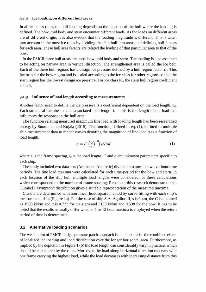
3.1.3 Influence of load length according to measurements
Another factor used to define the ice pressure is a coefficient dependent on the load length, ca.
Each structural member has an associated load length la – this is the length of the load that
influences the response in the hull area.
The function relating measured maximum line load with loading length has been researched
on e.g. by Suominen and Kujala (2015). The function, defined in eq. (1), is fitted to multiple
ship measurement data to render curves denoting the magnitude of line load q as a function of
load length.
𝑞 = 𝐶 (𝑙𝑐𝑠
)−𝑎
[kN/m] (1)
where s is the frame spacing, lc is the load length, C and a are unknown parameters specific to
each ship.
The study included two data sets (Arctic and Antarctic) divided into one and twelve-hour time
periods. The line load maxima were calculated for each time-period for the bow and stern. In
each location of the ship hull, multiple load lengths were considered for these calculations
which corresponded to the number of frame spacing. Results of this research demonstrate that
Gumbel I asymptotic distribution gives a suitable representation of the measured maxima.
C and a are determined with non-linear least square method by curve-fitting with each ship’s
measurement data (Figure 1a). For the case of ship S.A. Agulhas II, s is 0.4m, the C is obtained
as 1989 kN/m and a is 0.733 for the stern and 3150 kN/m and 0.538 for the bow. It has to be
noted that the results naturally differ whether 1 or 12 hour maxima is employed when the return
period of time is determined.
3.2 Alternative loading scenarios
The weak point of FSICR design pressure patch approach is that it excludes the combined effect
of localized ice loading and load distribution over the longer horizontal area. Furthermore, as
implied by the depiction in Figure 1 (b) the load length can considerably vary in practice, which
should be considered by the rules. Moreover, the load along horizontal direction can vary with
one frame carrying the highest load, while the load decreases with increasing distance from this

Loading
frame. The latter notion is supported also by measurements conducted on icebreaker Sisu
(Kujala and Vuorio, 1986).
Figure 1. a) Maximum line loads determined from full-scale ship measurements (three ships) as a function of load
length (Suominen and Kujala, 2015) – Return period taken is 10 days. b) Sketch of ice contact with ship structure – may describe an event that is only centimeters across, or it may be meters across, Daley (2007).
3.2.1 Load length effect
The present FSICR approach assumes that load is equally distributed between framing members
and in direct analysis with FEM, pressure patch length equals the webframe spacing; e.g., see
Figure 2, case 8s. To determine the effect of patch length on capacity of the frames four different
loading scenarios are considered besides the uniform pressure patch of FSICR as shown in
Figure 2. The length of the patch is decreased from webframe spacing (FSICR, denoted as 8s)
to one frame spacing (1s). Furthermore, in the last case study a scenario is proposed where
pressure is uniform over a frame spacing, but decreases exponentially outside this area as de-
fined with eq. (1). This case is denoted as non-uniform pressure patch – NUPP.
𝑝 = {
8.7(7.175 − 𝑥)−0.733 𝑖𝑓 𝑥 < 6.28518.8 𝑖𝑓 6.825 ≤ 𝑥 ≤ 7.175
8.7(𝑥 − 6.825)−0.733 𝑖𝑓 𝑥 > 7.715
(2)
In contrast to FSICR, NUPP considers the fact that that ice load will have some local character
in the middle, but also accounts the decreasing load character that is consistent with measure-
ments shown in Figure 1 (a). This local charater is especially important when considering over-
load situations to which we focus in this report.
The pressure values shown in Figure 2 were chosen based on preliminary simulations so that
plastic deformations would take place in the structure. Since in the simulations pressure is
ramped up from zero to maximum the presented values are the maximum attained. The ad-
vantage of ramping procedure is that pressure can be treated as a variable when results are
analyzed. Details of pressure application are presented in the next section.

Figure 2. Pressure patches used in the investigation
3.2.2 Effect of load height
As the ship penetrates into an ice sheet, the ice edge is crushing and a nominal contact area is
increasing – the process is depicted in Figure 3 (b) and its adoption is also basis for current
design pressure patch height. The crushing of ice continues until the bending failure of the ice
sheet. However, there is an aboundance of evidence that crushing phase contains an intermedi-
ate phenomenon whereby a “line-like” contact developes from adjacent of high pressure zones
distributed over the contact region. The resulting scenario is also proposed as a possible future
design scenario, see Figure 3 (c).
The pressure values measured in those localized zones can be as high as ~50 MPa, as opposed,
ice pressure in FSICR is never higher than 5.6 MPa. This striking difference represents a sig-
nificant gap in the knowledge and thus, also in the rules, which can only be addressed by seam-
less intertwining of experimental testing and numerical simulations. Current study focuses on
the latter as simulations allow us to separate the individual and interactive effects of factors that
have most deteriorating effect on the structural behaviour. Therfore, one of those individual
effects we focus is load height, besides the load length.
Figure 3. Load height development in FSICR (Riska and Kämäräinen, 2012).
FE analyses
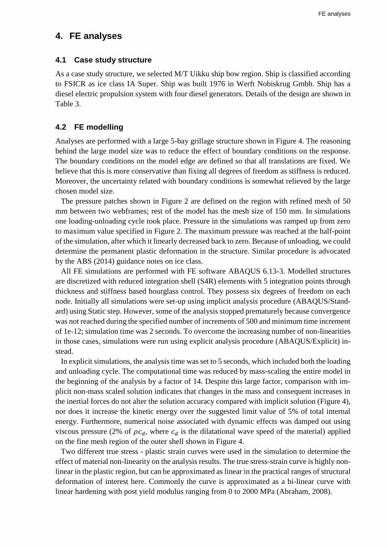
4. FE analyses
4.1 Case study structure
As a case study structure, we selected M/T Uikku ship bow region. Ship is classified according
to FSICR as ice class IA Super. Ship was built 1976 in Werft Nobiskrug Gmbh. Ship has a
diesel electric propulsion system with four diesel generators. Details of the design are shown in
Table 3.
4.2 FE modelling
Analyses are performed with a large 5-bay grillage structure shown in Figure 4. The reasoning
behind the large model size was to reduce the effect of boundary conditions on the response.
The boundary conditions on the model edge are defined so that all translations are fixed. We
believe that this is more conservative than fixing all degrees of freedom as stiffness is reduced.
Moreover, the uncertainty related with boundary conditions is somewhat relieved by the large
chosen model size.
The pressure patches shown in Figure 2 are defined on the region with refined mesh of 50
mm between two webframes; rest of the model has the mesh size of 150 mm. In simulations
one loading-unloading cycle took place. Pressure in the simulations was ramped up from zero
to maximum value specified in Figure 2. The maximum pressure was reached at the half-point
of the simulation, after which it linearly decreased back to zero. Because of unloading, we could
determine the permanent plastic deformation in the structure. Similar procedure is advocated
by the ABS (2014) guidance notes on ice class.
All FE simulations are performed with FE software ABAQUS 6.13-3. Modelled structures
are discretized with reduced integration shell (S4R) elements with 5 integration points through
thickness and stiffness based hourglass control. They possess six degrees of freedom on each
node. Initially all simulations were set-up using implicit analysis procedure (ABAQUS/Stand-
ard) using Static step. However, some of the analysis stopped prematurely because convergence
was not reached during the specified number of increments of 500 and minimum time increment
of 1e-12; simulation time was 2 seconds. To overcome the increasing number of non-linearities
in those cases, simulations were run using explicit analysis procedure (ABAQUS/Explicit) in-
stead.
In explicit simulations, the analysis time was set to 5 seconds, which included both the loading
and unloading cycle. The computational time was reduced by mass-scaling the entire model in
the beginning of the analysis by a factor of 14. Despite this large factor, comparison with im-
plicit non-mass scaled solution indicates that changes in the mass and consequent increases in
the inertial forces do not alter the solution accuracy compared with implicit solution (Figure 4),
nor does it increase the kinetic energy over the suggested limit value of 5% of total internal
energy. Furthermore, numerical noise associated with dynamic effects was damped out using
viscous pressure (2% of 𝜌𝑐𝑑, where 𝑐𝑑 is the dilatational wave speed of the material) applied
on the fine mesh region of the outer shell shown in Figure 4.
Two different true stress - plastic strain curves were used in the simulation to determine the
effect of material non-linearity on the analysis results. The true stress-strain curve is highly non-
linear in the plastic region, but can be approximated as linear in the practical ranges of structural
deformation of interest here. Commonly the curve is approximated as a bi-linear curve with
linear hardening with post yield modulus ranging from 0 to 2000 MPa (Abraham, 2008).
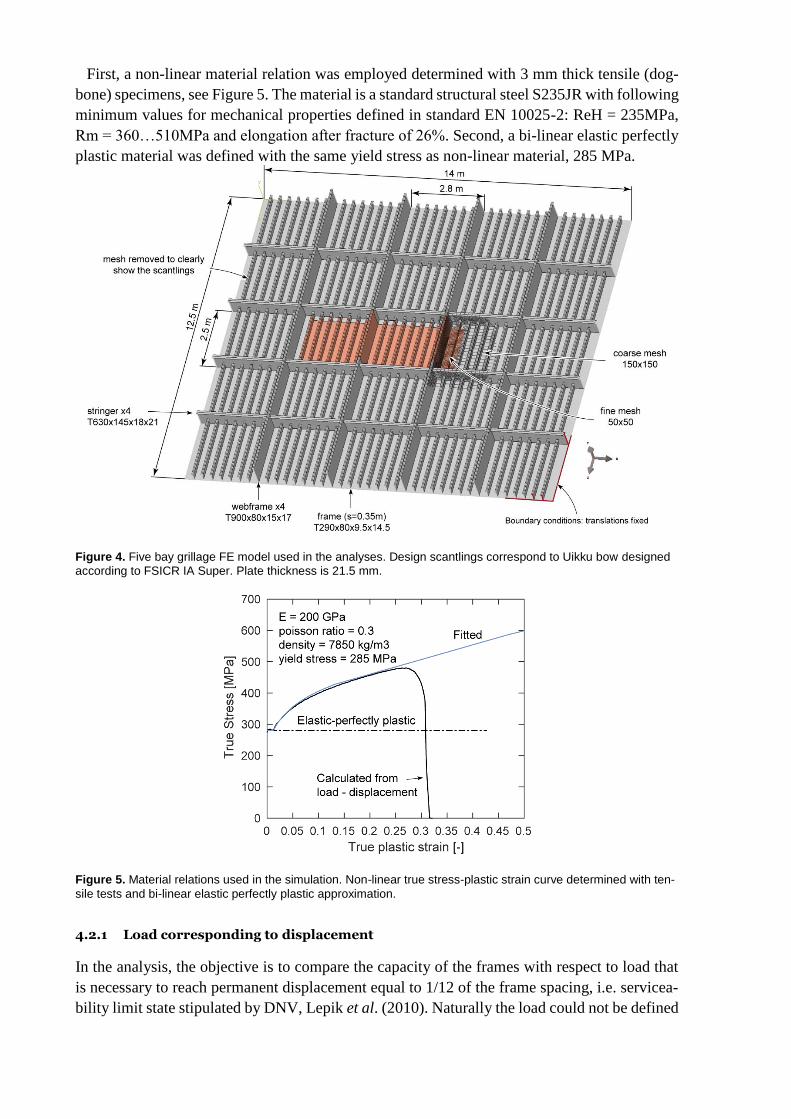
First, a non-linear material relation was employed determined with 3 mm thick tensile (dog-
bone) specimens, see Figure 5. The material is a standard structural steel S235JR with following
minimum values for mechanical properties defined in standard EN 10025-2: ReH = 235MPa,
Rm = 360…510MPa and elongation after fracture of 26%. Second, a bi-linear elastic perfectly
plastic material was defined with the same yield stress as non-linear material, 285 MPa.
Figure 4. Five bay grillage FE model used in the analyses. Design scantlings correspond to Uikku bow designed
according to FSICR IA Super. Plate thickness is 21.5 mm.
Figure 5. Material relations used in the simulation. Non-linear true stress-plastic strain curve determined with ten-
sile tests and bi-linear elastic perfectly plastic approximation.
4.2.1 Load corresponding to displacement
In the analysis, the objective is to compare the capacity of the frames with respect to load that
is necessary to reach permanent displacement equal to 1/12 of the frame spacing, i.e. servicea-
bility limit state stipulated by DNV, Lepik et al. (2010). Naturally the load could not be defined

FE analyses
a priori so that after unloading permanent set is exactly equal to the reference limit state. That
is why the pressure defined in Figure 2 is relatively large.
To determine the load corresponding to certain displacement we shifted the unloading portion
of the curve so that the permanent set would be exactly equal to the reference permanent dis-
placement as shown in Figure 60. The underlying assumption is that slope of the unloading
portion of the curve remains the same due to the permanent nature of plastic strains. This as-
sumption of similarity in unloading slope is verified with simulation where maximum pressure
was decreased (case 3s, new max. pressure 5 MPa) in Figure 6 – the two slopes, calculated and
shifted, overlap.
Figure 6. Comparison of implicit and explicit solution together with curve shifting verification. Results correspond
to loading case 3s performed with non-linear material. Implicit simulation stopped before unloading stage started. Total load corresponds to resultant force in the boundaries. Load on frame is obtained by integrating the pressure over the single frame spacing.
4.3 Load length effect on response
Analyses results are shown in Figure 7 where load on a single frame is plotted as a function of
displacement. Load on a single frame, that is for the one frame spacing, was found by integrat-
ing the applied pressure over the corresponding area. Displacements were measured at the two
locations: 1) where it was highest in the plate field (Figure 7 a), and 2) in the plate field at the
frame location (Figure 7 b). The capacity of the frames is compared with respect to load that is
necessary to reach permanent displacement equal to 1/12 of the frame spacing, i.e. serviceabil-
ity limit state stipulated by DNV. The procedure is described in previous section.
The results in Figure 70 (a) demonstrate that material non-linearity has negligible influence
on the response in the range of structural deformations considered. The reason is that plastic
strains remain small in the range below 5% at the permanent displacement limit used here, for
example, see Figure 8. Using bi-linear material reduces the analysis set-up time, but the range
of deformations where this simplification remains valid should be determined.

Figure 7. Load on single frame as a function of displacement. Displacement at (a) middle of the plate field and (b)
on the plate field at the frame location. For each case load causing the permanent deformation of s/12 is high-lighted.
Figure 8. Excerpt of the structure under 3s patch at the instance when load on frame is 857 kN. Plastic strains
remain under 4%.
Comparison of Figure 7 (a) and (b) shows that slightly stiffer response is obtained when defor-
mations are measured at the frame location. But as the effect is negligible we focus on results
presented in Figure 7 (a).
Results in Figure 7 (a) imply that capacity considerably reduces with increasing load length,
rendering the current design approach the most critical (8s). But the impression is deceiving as
the external loading acting outside the single frame spacing clearly reduces the structural stiff-
ness of individual frames.
Therefore, to account for this effect we convert the determined load, Fframe, into format of line
load and present it as a function of load length. For uniform load the calculated line load is
𝑞𝑢𝑛 = 𝐹𝑓𝑟𝑎𝑚𝑒/𝑠 (3)
where s is the frame spacing. For non-uniform load, the line load is found by integrating the
pressure function given by eq. (1) and by normalizing it to account for the fact that Fframe was
reached before maximum applied load was reached in the simulation
𝑞𝑛𝑢 =ℎ
𝐿∫ 𝑝(𝑥)𝑑𝑥
8.4
5.6
∙𝐹𝑓𝑟𝑎𝑚𝑒
ℎ ∫ 𝑝(𝑥)𝑑𝑥7.175
6.825
(4)

FE analyses
=ℎ
𝐿∫ 𝑝(𝑥)𝑑𝑥
8.4
5.6
∙𝐹𝑓𝑟𝑎𝑚𝑒
18.8 ∙ ℎ ∙ 𝑠
where h = 0.35 m is the height of the patch, and L = 2.8 m is the length of the patch. The results
are presented in Table 2. The obtained line load is also plotted against full-scale ship measure-
ment data in Figure 9 for two ships. Although the measurement data applies to different struc-
tures, the comparison shows that the trend of the obtained results is consistent with the measured
values. Qualitatively, the most critical loading scenarios are the ones in which percentage dif-
ference with measurements is smallest – cases 2s and 3s; in this comparison, we selected Agul-
has II ship whose measurements better correlate with the calculated values. This percentage is
also given in Table 2.
These results show that both the length of the pressure patch and the non-uniformity of pres-
sure play an important role in determining the plastic capacity of the frames and thus, also the
whole structure. If the shift in rules is made towards allowance of plastic limit states future
FSICR rules should aspire to the patch definition that yields the most conservative results –
largest damage with the least applied load. Comparison of critical line load values with the
measured values in Figure 9 indicates that the current FSICR design approach is not the most
critical scenario. Narrower patches or non-uniform pressure distribution are qualitatively more
critical. Important perspective considering that recent findings indicate that load has to be in
the range of (1-4 frame spacings) in order for the maximum load on a frame to occur, Suominen
et al. (2017).
Table 2. Load on single frame to reach the permanent displacement equal to 1/12 of the frame spacing.
Figure 9. Line load – load length relationship determined from full-scale ship measurements (Suominen and
Kujala, 2015). Return period taken is 10 days.
4.4 Effect of material hardening – large deformations
The effect of material hardening on the large deformation behaviour is further investigated, by
using NUPP pressure patch on Uikku IA Super bow grillage.
Casesolver
Load
length[m]
Loadonframe
[kN](F_frame)
Lineloadq1
[kN/m]
q2[kN/m]
Agulhassbow
(q1-q2)/q2
[%]
1s implicit 0.35 1870 5343 3385 58%
2s implicit 0.7 1158 3309 2331 42%
3s explicit 1.05 857 2449 1874 31%
8s explicit 2.8 690 1971 1106 78%
NU implicit 2.8 967 1623 1106 47%

The results of the analysis in Figure 10 (a) indicate that material hardening has negligible
effect on the frame response, at least during majority of the response. This material insensitivity
in large grillage is attributed to the structures ability to effectively distribute loads. Essentially
there are two competing mechanisms taking place – material hardening and structural softening.
Material hardening associated with localized plastic deformation remains so localized that it
has negligible effect on the overall load-displacement response. To confirm this hypothesis
analyses were performed also with an isolated frame, again using the same two material models.
Figure 10 (b) reveals that in isolated frame the material has a stronger role on response.
Going back to large grillage, the closer inspection of deformed structures revealed an im-
portant disparity between two material modelling approaches at later stages of analysis, see
Figure 11 where development of plastic strain is plotted in different stages of analysis. In sim-
ulations with non-linear material the hardening promotes distribution of stresses and plastic
strains as opposed to local material deformation that requires more energy. In contrast, such
mechanism is missing in simulations with bi-linear material. Plastic strains localize in frame
flanges with very little spread that in turn leads to eventual neck development and failure. Fur-
thermore, the inability to spread the stresses leads also to different structural behaviour with
frames tripping and folding in simulations with non-linear material, but remaining straight in
bi-linear material simulation.
Figure 10. The effect of material non-linearity on Uikku bow frame response. a) Grillage and b) isolated frame.

FE analyses
Figure 11. Effect of material non-linearity on plasticity spread in structures.
4.5 Effect of load height
To test the effect of load height on the analysis results two patch heights are considered: 35 cm
consistent with IA Super current design patch and 10 cm height. Again, the structure of Uikku
bow IA Super is employed for the analysis. The pressure distribution in the horizontal direction
was non-uniform according to NUPP with the length of webframe distance defined in previous
section.
Simulations were set-up so that the total load would be equal in both cases, which implies that
the pressure applied through the narrower patch is about 3.5 times higher. In terms of the whole
structure, this pressure difference has negligible effect on response as shown in Figure 12 (a).
Much more revealing insight is obtained when inspecting the single frame response in Figure
12 (b). Under the same nominal load, the localization created by the “line-like” load signifi-
cantly reduces the capacity of the frame. The load on frame causing permanent deformation of
~50 mm is about two times lower than manifested through patch with height of 35 cm.
As the effect of load height prominently reduces the capacity of the frames, more compelling,
experimental insight is needed before enforcing load height change in rules. Therefore, the fol-
lowing analysis are performed with load height consistent with the current rules.

Figure 12. Effect of patch height on the response. a) Effect on structure and b) on single frame.
5. Fracture limit state
The objective of this section is to determine how and where fracture takes place in side structure
under distributed pressure load. Although the load corresponding to the pressure patch area
might be unrealistically high, the analyses are in agreement with the current best practice and
are still believed to give important insight regarding fracture behaviour as well as structural
behaviour prior to failure. Furthermore, of interest are the load values at which fracture takes
place so these can be compred with values presented in Table 5.
5.1 FE simulations including fracture
Fracture in the material was modeled by deleting elements when fracture strain, independent of
stress state, was reached. Although fracture strain in metals strongly depends on the stress state,
this coarse assumption is justified by the fact that the objective here is to determine the structural
component prone to fracture initiation under pressure loads in contrast to fracture propagation
analysis. Fracture strain was scaled with element size. There are several equations developed
for this purpose. Usually they are based on Barba’s relation that is formulated as follows
(Hogström 2009)
(5)
Here, εf is fracture strain, εn (0.2) equals to necking strain of the material estimated from engi-
neering stress-strain curve, c (0.164, determined from fit on data) is the Barba parameter and
W (15mm) and t (3mm) represent original width and thickness of flat tensile test specimen,
respectively. LVE is the length of the virtual extensometer (VE) over which fracture strain is
measured in a tensile test. For 50 mm elements used in the present investigation, eq. (5) yields
a fracture strain of 0.26.
Analyses were performed with Uikku mid-section model designed according to IAS and IB
ice classes. The results are presented in Figure 13. In both cases fracture initates in the frame
flange, whereas at the point of failure plastic strain in the outer shell is around 14%. The dis-
placement to failure is ~0.5 m, which compared to the permanent deflection limit state used in

Frame response
previous section (30 mm) is about 16 times higher. Load to fracture in case of IAS is ~2500 kN
is about 5 times higher, again compared with permanent deflection LS.
Figure 13. Fracture initiation in structure under pressure load
In above simulations, the middle stiffener remained almost straight exhibiting no tripping nor
folding to the sides. This was the main reason which led to high tensile strains in the stiffener
flange that ultimately caused the fracture there. Since such a symmetry is almost impossible in
reality, another, more probable scenario was analyzed where asymmetry was evoked by off-
setting the load 150 mm towards webframe.
Figure 13 clearly shows how irregularity of the load with respect to the frame location is
detrimental to the capacity. In both ice classes also fracture load was slightly lower. The most
captivating, however, is the fact that for irregular load the fracture took place in the outer shell,
rather than in the frames.
6. Frame response
In this section, the behaviour of frames is studied more extensively with the proposed loading
scenario as it yields more structural damage and is thus less conservative. Besides Uikku ship,
analyses are performed with S.A. Agulhass II. We performed analyses with three ice classes
(IA Super, IA and IB) and considered three hull regions: bow, mid and stern.
6.1 Analyzed ship structures
The main particulars of both ships are given in Table 3. The reason why these ships were se-
lected was that the ships were intrumented with strain gages and thus, there exist experimental
data we can later compare our analysis results.
S.A. Agulhas II in Figure 14 (a) was built to be classified as Polar ice class PC5 and the hull
was constructed in accordance with DNV ICE-10. For the structural scantlings of bow, mid-
ship and stern, T-frames are used. The frame span for the bow is 2.065 m and 1.1 m for the
mid-ship and stern. The frame spacing and webframe spacing for bow, mid-ship and stern is
0.4 m and 2.4 m respectively. Three areas of the starboard side of the hull were instrumented
with strain gauges when it was under construction in 2011/2012. Ice-induced loads were deter-
mined by instrumenting the upper and lower parts of the frame with V-shaped strain gauges,

which measured the shear strains occurring in the frame. The instrumentation was applied to
two adjacent frames at the bow, three adjacent frames at the bow-shoulder and four adjacent
frames at the stern-shoulder. In addition, the hull plating was instrumented with strain gauges
in these areas. See Suominen et al. (2013) for more detailed description of the instrumentation.
M/T Uikku in Figure 14 (b), on the other hand, is classified by DNV as class +1 A Tanker for
Oil and according to FSICR, it is classified as ice class IA Super. Ship was built in 1976 in
Werft Nobiskrug Gmbh, and Helsinki New Shipyard rebuilt Azipod conversion 1993. The ship
has a diesel electric propulsion system with four diesel generators. The ship hull and propulsion
system was instrumented in 1997 for the EU funded ARCDEV project and the instrumentation
was extensive. Measurements were performed on the shell transverse frame at bow area, at bow
shoulder area, at midship area and at aftship area (measured by shear strain gauges), load on
the shell longitudinal frames at midship area (measured by shear strain gauges), stresses on the
shell plating and frames at waterline at bow area, at bow shoulder area, at midship area and at
aftship area, the longitudinal bending stresses on deck and vertical accelerations at the bow and
stern of the ship and longitudinal acceleration at bow. Thereby, the ice loads were evaluated by
measuring shear strains at roughly the neutral axis of the frame. The scantling information for
both ships are summarized in the tables below. More detail description of the instrumentation
can be found in Kotisalo and Kujala (1999). The frame span for the bow is 2 m, 2.92 m for the
bow-shoulder and 1.22 m for the stern, and the frame spacing is 0.35 m.
Table 3. The main particulars of two ships
(a)
Ship Length Breath Design draught Deadweight DisplacementService
speedPower
S.A. Agulhass II 121.8 21.7 7.65 5000 13632 14 kn 9 MW
Uikku 150 m 22.2 m 9.5 m 15748 t 22654 t 17 kn 11.4 MW

Frame response
(b)
Figure 14. Pictures of two ships for which measurement data is available.
6.1.1 Approach
The large number of analysis performed required a systematic approach. The process is outlined
in Figure 15. The ships have been re-dimensioned to comply with the FSICR requirements.
This was done for three ice classes (IA Super, IA and IB) and three hull regions: bow, mid and
stern. Scantlings were calculated using FSICR equations and each ship’s input dimensions, see
Table 4. During scantlings calculations, the brackets have been assumed to be non-existent in
the models. Using the obtained scantlings from Matlab, Abaqus python module has been used
to build parametric finite element models of both ships. These parametric features provide the
swift ability to examine the effects of design changes. Using parametric modeling, a finite ele-
ment model and its mesh characteristics can be completely defined in terms of parameters or
variables. A finite element parametric modeling method of ships overcomes the time-consum-
ing aspect of finite element analysis pre-processing which makes exploring the design space
very effective. Furthermore, these scripts are published together with this report which makes
them accessible in future investigations.
Thin shell elements have been used to model frames, plating, web frames, flanges and stiff-
eners. Although stringer and web span are slightly different for both ships, all models include
5 bays in both longitudinal and transverse direction as shown in Figure 4.
Figure 15. Flow diagram of analysis steps
Table 4. Calculated scantlings for both ships according to FSICR. Yield stress assumed in calculations is 285 MPa.

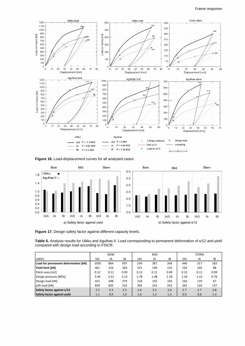
6.2 Frame analysis results
The results for all analysed cases are shown in Figure 16 presented in the form of load on single
frame plotted as a function of displacement. The load on a single frame was preferred over a
total load as a comparative measure because this is also available from measurements facilitat-
ing the comparison in the sequel. Load on a single frame, that is for one frame spacing, was
found by integrating the applied pressure over the corresponding area. Displacements were
measured in the plate field at the frame location. The permanent deformations in the structures
were determined by assuming that the slope of the unloading curve remains the same due to the
permanent nature of plastic strains. Thereby, the unloading portion of the curve is shifted to-
wards left along the x-axes as shown in Figure 6 so that the permanent set would be exactly
equal to the reference permanent displacement.
In general, stiffness reduction correlates with the decrease in ice class as well as hull region –
this is consistent with the current design approach. On the curves, three distinctive points are
marked: load to permanent deformation s/12, design load according to the FSICR and three
hinge pressure load (Daley, 2002). Furthermore, from FE simulations we could determine the
yield point in each analysis. All the results are combined in Table 5.
The yield capacity is reached before permanent deformation. The last line in Table 5 gives
the ratio between the yield load and the design load, i.e. the safety factor against yield – this is
presented also in Figure 17 (a). The closer the safety factor is to 1 the more successfully the
structure follows the design intention of the FSICR that is reaching the state of yielding when
subjected to design pressure. Uikku follows the design intention surprisingly well. The midship
and stern regions of Agulhas II are slightly over-dimensioned. The safety factor against perma-
nent deformation of s/12 is larger than ~2.5.
Bow Plating Power
t[mm] h_web t_web w_flange t_flange h_web t_web w_flange t_flange h_web t_web w_flange t_flange P[kW]
IAS 21.5 260 9.5 80 12.5 660 18 140 20 900 15 80 17 11400
IA 20 260 9 70 11.5 580 16 145 21 700 15 60 15 6614
IB 19 240 9 70 11.5 540 17 120 18 650 15 80 15 5300
Mid Plating Power
t[mm] h_web t_web w_flange t_flange h_web t_web w_flange t_flange h_web t_web w_flange t_flange P[kW]
IAS 16 190 9 70 11.5 500 10 60 14 550 13 80 16 11400
IA 15 170 9 70 11.5 450 8 55 14 450 12 60 15 6614
IB 12.5 140 9 70 11.5 350 9 60 13 350 12 60 15 5300
Stern Plating Power
t[mm] h_web t_web w_flange t_flange h_web t_web w_flange t_flange h_web t_web w_flange t_flange P[kW]
IAS 14 120 9 40 11.5 450 8 60 14 500 10 80 16 11400
IA 11.5 100 9 50 10 340 8 80 14 380 10 80 16 6614
IB 10 80 9 40 10 290 10 40 10 290 10 40 10 5300
Bow Plating Power
t[mm] h_web t_web w_flange t_flange h_web t_web w_flange t_flange h_web t_web w_flange t_flange P[kW]
IAS 22.5 290 10.5 80 16 600 17 80 21 700 15 80 17 9000
IA 18.5 210 10 80 15 500 14 75 18 600 12 60 16 4941
IB 16 170 10 80 15 400 14 70 18 500 12 50 15 3478
MID Plating Power
t[mm] h_web t_web w_flange t_flange h_web t_web w_flange t_flange h_web t_web w_flange t_flange P[kW]
IAS 17 210 10 80 15 500 15 70 17 500 12 70 15 9000
IA 15 170 10 80 15 400 13 70 16 450 9 60 12 4941
IB 13 140 10 80 15 350 12 60 14 400 8 55 10 3478
Stern Plating Power
t[mm] h_web t_web w_flange t_flange h_web t_web w_flange t_flange h_web t_web w_flange t_flange P[kW]
IAS 15 170 10 80 15 400 14 70 17 400 12 70 15 9000
IA 13 140 10 80 15 350 12 70 16 400 9 60 12 4941
IB 10.5 120 10 80 15 300 9 60 13 300 7 45 9 3478
UIKKU
Agulhas
Frames[mm](spacing=0.35m) stringer[mm](spacing=2m) webframe[mm](spacing=2.8m)
Frames[mm](spacing=0.35m) stringer[mm](spacing=2m) webframe[mm](spacing=2.1m)
Frames[mm](spacing=0.4m) stringer[mm](spacing=1.1m) webframe[mm](spacing=2.4m)
Frames[mm](spacing=0.4m) stringer[mm](spacing=1.1m) webframe[mm](spacing=2.4m)
Frames[mm](spacing=0.4m)
Frames[mm](spacing=0.35m) stringer[mm](spacing=1.22m) webframe[mm](spacing=2.1m)
stringer[mm](spacing=2.065m) webframe[mm](spacing=2.4m)
Frame response
Figure 16. Load-displacement curves for all analysed cases.
Figure 17. Design safety factor against different capacity levels.
Table 5. Analysis results for Uikku and Agulhas II. Load corresponding to permanent deformation of s/12 and yield compared with design load according to FSICR.
ENGINEPOWERCASE UIKKU IAS IA IB IAS IA IB IAS IA IB
Loadforpermanentdeformation[kN] 1050 804 697 534 387 264 446 317 183
Yieldlimit[kN] 461 316 263 221 190 132 154 105 88
Patcharea[m2] 0.12 0.11 0.09 0.12 0.11 0.09 0.12 0.11 0.09
Designpressure[MPa] 3.44 3.31 3.13 1.78 1.48 1.18 1.34 1.13 0.76
Designload[kN] 421 348 274 218 155 103 164 119 67
p3hload[kN] 839 602 532 393 333 253 265 210 137
Safetyfactoragainsts/12 2.5 2.3 2.5 2.4 2.5 2.6 2.7 2.7 2.8
Safetyfactoragainstyield 1.1 0.9 1.0 1.0 1.2 1.3 0.9 0.9 1.3
BOW STERNMID
7. Description of full scale measurements
The ice load is determined with the full-scale observations onboard two vessels: Research ves-
sel SA Agulhas II in Antarctica and tanker Uikku in the Russian Arctic. Table 3 and Table 4
summarise the main characteristics of the vessels and Figure 14 illustrates the ships.
7.1 Description of the measuring voyage
7.1.1 SA Agulhas II
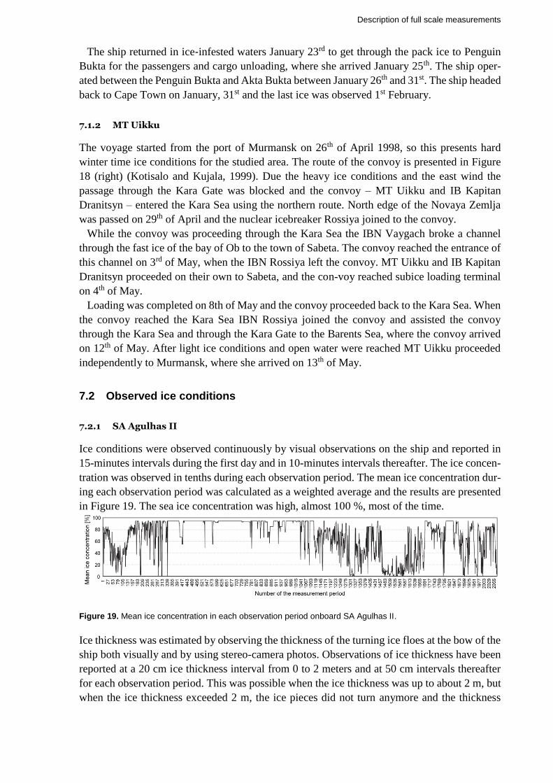
Full scale measurement data on ice conditions was collected in the Antarctic waters onboard
S.A. Agulhas II between Dec 6, 2013 and Feb 2, 2014. The ice conditions were observed visu-
ally and the machinery control and navigational data were recorded continuously. The ice‐in-
duced loads were also measured at the bow, bow shoulder and stern shoulder of the ship hull.
Figure 18. Left: Sea ice extent on Antarctica on 7th December 2013. Right: Route of the convoy during ARCDEV voyage.
The ship departed Cape Town on November 28th, 2013 (Suominen et al., 2015a, 2015b). From
Cape Town, the ship headed to the zero Meridian, which she followed to Antarctica, see Figure
18. The first time the ship encountered ice was on December 7th. On December 23rd, the ship
arrived the Akta Bukta close to the Neumayer III (the German Antarctic research station, see
Figure 18 left).
Between December 24th and 30th, the ship operated between the Akta Bukta and the Penguin
Bukta (the location at the ice shelf with the shortest distance to the South African Antarctic
research station, SANAE IV, see Figure 18 left) close the ice shelf. On December 30th, the ship
headed towards South Georgia and the South Sandwich Islands. The ship arrived at the South
Sandwich Islands January 4th when also the extent of sea ice ended.
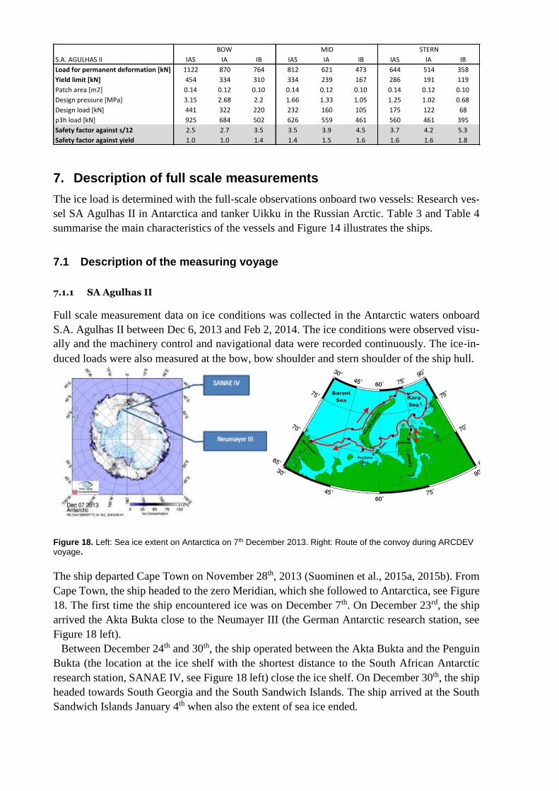
S.A.AGULHASII IAS IA IB IAS IA IB IAS IA IB
Loadforpermanentdeformation[kN] 1122 870 764 812 621 473 644 514 358
Yieldlimit[kN] 454 334 310 334 239 167 286 191 119
Patcharea[m2] 0.14 0.12 0.10 0.14 0.12 0.10 0.14 0.12 0.10
Designpressure[MPa] 3.15 2.68 2.2 1.66 1.33 1.05 1.25 1.02 0.68
Designload[kN] 441 322 220 232 160 105 175 122 68
p3hload[kN] 925 684 502 626 559 461 560 461 395
Safetyfactoragainsts/12 2.5 2.7 3.5 3.5 3.9 4.5 3.7 4.2 5.3
Safetyfactoragainstyield 1.0 1.0 1.4 1.4 1.5 1.6 1.6 1.6 1.8
BOW STERNMID
Description of full scale measurements
The ship returned in ice‐infested waters January 23rd to get through the pack ice to Penguin
Bukta for the passengers and cargo unloading, where she arrived January 25th. The ship oper-
ated between the Penguin Bukta and Akta Bukta between January 26th and 31st. The ship headed
back to Cape Town on January, 31st and the last ice was observed 1st February.
7.1.2 MT Uikku
The voyage started from the port of Murmansk on 26th of April 1998, so this presents hard
winter time ice conditions for the studied area. The route of the convoy is presented in Figure
18 (right) (Kotisalo and Kujala, 1999). Due the heavy ice conditions and the east wind the
passage through the Kara Gate was blocked and the convoy – MT Uikku and IB Kapitan
Dranitsyn – entered the Kara Sea using the northern route. North edge of the Novaya Zemlja
was passed on 29th of April and the nuclear icebreaker Rossiya joined to the convoy.
While the convoy was proceeding through the Kara Sea the IBN Vaygach broke a channel
through the fast ice of the bay of Ob to the town of Sabeta. The convoy reached the entrance of
this channel on 3rd of May, when the IBN Rossiya left the convoy. MT Uikku and IB Kapitan
Dranitsyn proceeded on their own to Sabeta, and the con-voy reached subice loading terminal
on 4th of May.
Loading was completed on 8th of May and the convoy proceeded back to the Kara Sea. When
the convoy reached the Kara Sea IBN Rossiya joined the convoy and assisted the convoy
through the Kara Sea and through the Kara Gate to the Barents Sea, where the convoy arrived
on 12th of May. After light ice conditions and open water were reached MT Uikku proceeded
independently to Murmansk, where she arrived on 13th of May.
7.2 Observed ice conditions
7.2.1 SA Agulhas II
Ice conditions were observed continuously by visual observations on the ship and reported in
15-minutes intervals during the first day and in 10-minutes intervals thereafter. The ice concen-
tration was observed in tenths during each observation period. The mean ice concentration dur-
ing each observation period was calculated as a weighted average and the results are presented
in Figure 19. The sea ice concentration was high, almost 100 %, most of the time.
Figure 19. Mean ice concentration in each observation period onboard SA Agulhas II.
Ice thickness was estimated by observing the thickness of the turning ice floes at the bow of the
ship both visually and by using stereo-camera photos. Observations of ice thickness have been
reported at a 20 cm ice thickness interval from 0 to 2 meters and at 50 cm intervals thereafter
for each observation period. This was possible when the ice thickness was up to about 2 m, but
when the ice thickness exceeded 2 m, the ice pieces did not turn anymore and the thickness

estimation was more complicated. Thick snow cover made also the thickness observations dif-
ficult. Figure 20 shows the observed mean ice thickness for each period.
Figure 20. Mean ice thickness in each observation period onboard SA Agulhas II
Most of the time, the level ice thickness encountered at a certain 10-minutes observation period
varied quite much. Typically, 4 to 6 different ice thicknesses were observed during each 10-
minutes periods. Obviously, the ice fields are often moving out to the open sea from Antarctica
due to the wind, waves and currents and therefore the level ice field is broken into ice floes.
New ice is then formed between the broken ice floes, which can explain the existence of differ-
ent thicknesses of level ice at open sea.
Figure 21. The speed of SA Agulhas II during each 10-minutes period.
Figure 21 illustrates the ship’s speed during the voyage. As can be seen, the ship had large
difficulties to get through the thick ice regime when approaching Akta Bukta before Christmas
2013. The ship was stuck a number of times, but got however slowly forward independently by
ramming through the thick ice.
7.2.2 MT Uikku
Ice conditions were observed continuously by visual observations on the ship and reported in
20 minutes intervals. The ice concentration was observed in tenths during each observation
period. The mean ice concentration during each observation period was calculated as a weighted
average and the results are presented in Figure 22.
Ice thickness was estimated by observing the thickness of the turning ice floes at the bow of
the ship visually. Observations of ice thickness have been reported on five classes: below 10
cm, 10-30 cm, 30-70 cm, 70-120 cm and above 120 cm. Figure 23 shows the observed mean
ice thick-ness for each period. Figure 24 illustrates the ship’s speed during the voyage. As can
be seen, the ship could keep fairly high speed of 10-15 kn most of the time as there were always
icebreakers to assist the ship.

Description of full scale measurements
Figure 22. Mean ice concentration in each observation period onboard MT Uikku.
Figure 23. Mean ice thickness in each observation period onboard MT Uikku.
Figure 24. The speed of MT Uikku during each 20-minutes period.
7.3 Evaluation of the design load
7.3.1 SA Agulhas II and MT Uikku
The measured 10-minute maximum loads at the bow and stern are used in this analysis. The
data is divided into 4 four classes using ice thickness as the criteria: smaller than 0.7 m, between
0.7-1.2 m, between 1.2-2.0 m and higher than 2.0 m (Kurmiste, 2016). Figure 25-27 summarise
the measured load and fitted Gumbel 1 distribution on the data. Gumbel 1 equations can be
presented:
𝐺(𝑦𝑛) = 𝛼𝑛𝑒−𝑒−𝛼𝑛(𝑦𝑛−𝑢𝑛) (6)
where Gumbel parameter 𝛼𝑛 is the inverse measure of dispersion and 𝑢𝑛 is the characteristic
largest value. These are determined based on the mean μ and standard deviation σ of the meas-
ured loads as follows:
𝛼𝑛 =𝜋
𝜎√6 (7)
𝑢𝑛 = 𝜇 −𝛾
𝛼𝑛 (8)
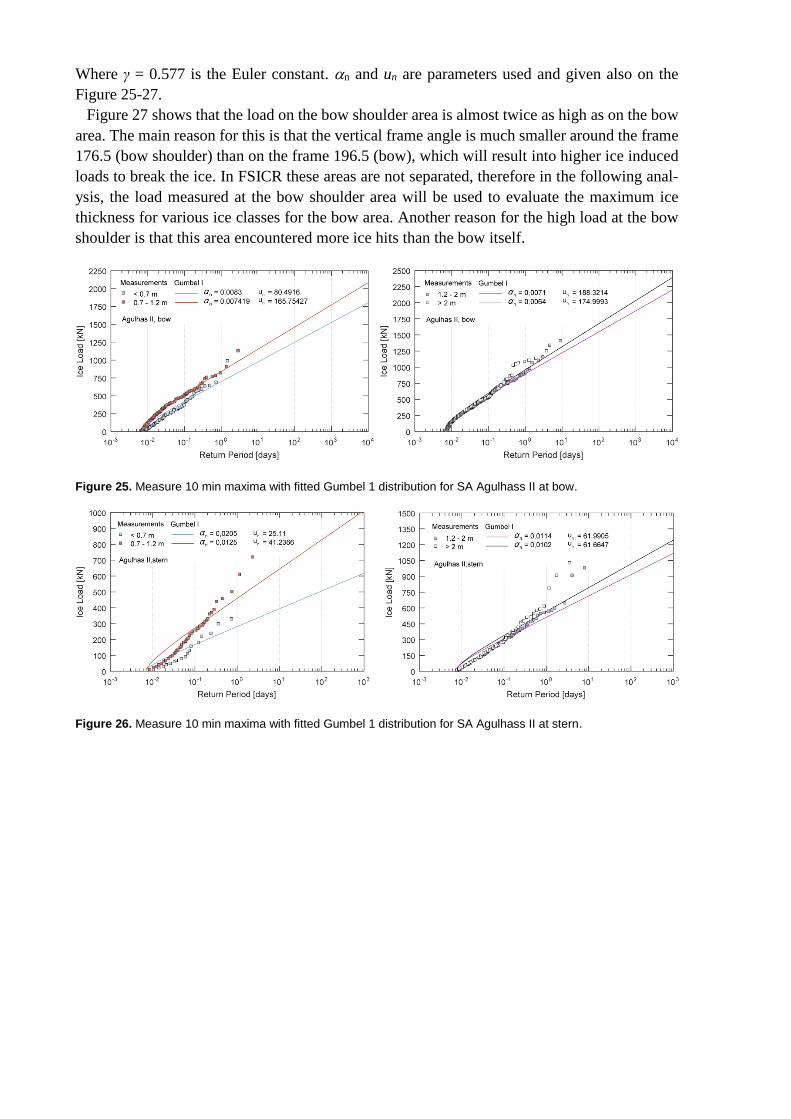
Where γ = 0.577 is the Euler constant. n and un are parameters used and given also on the
Figure 25-27.
Figure 27 shows that the load on the bow shoulder area is almost twice as high as on the bow
area. The main reason for this is that the vertical frame angle is much smaller around the frame
176.5 (bow shoulder) than on the frame 196.5 (bow), which will result into higher ice induced
loads to break the ice. In FSICR these areas are not separated, therefore in the following anal-
ysis, the load measured at the bow shoulder area will be used to evaluate the maximum ice
thickness for various ice classes for the bow area. Another reason for the high load at the bow
shoulder is that this area encountered more ice hits than the bow itself.
Figure 25. Measure 10 min maxima with fitted Gumbel 1 distribution for SA Agulhass II at bow.
Figure 26. Measure 10 min maxima with fitted Gumbel 1 distribution for SA Agulhass II at stern.

Description of full scale measurements
Figure 27. Measure 20 min maxima with fitted Gumbel 1 distribution for MT Uikku fro bow, bow shoulder and
stern.
7.4 Evaluation of the design load
The design of structures to withstand the ice loads has to take into account the stochastic nature
of this load. Therefore, a rational design procedure necessitates to use a statistical approach of
some sort.
Therefore, once the Gumbel parameters a and u are known, the most probable extreme value
with the probability of s, can be determined:
𝑦�̂� = 𝑢 − 𝑎−1 ln (− ln (1 −𝛼𝑠
𝑛)) (9)
Using eq. (8) and the data given in Figures 25-27, the most probable design load values during
one voyage (return period one day) are given for two safety levels, namely αs = 0.1 and αs = 1.
These safety factors are chosen as they comply with the latest standard for design of Arctic
offshore structures (ISO 19906:2010), which defines the three exposure categories and related
return period for the probability of occurrence of these:
1. Ultimate limit state (ULS) for all exposure levels (EL’s) requires extreme 100-year (10-2) ice event
with action factors dependent on the EL. ULS generally correspond to resistance to extreme
applied actions.
2. Abnormal/accidental limit state (ALS) for with 1,000 year (10-3) ice events allowing some
structural damage but robustness have to be achieved with no loss of life or harm to the
environment.
3. Serviceability (SLS) ensuring functionality under any 10 year (10-1) ice event. Exceedance of SLS
results in the loss of capability of a structure to perform adequately under normal use.

From the ones presented above we are using SLS criteria (αs = 0.1), which was also used pre-
viously to define the load values in Figure 16. Hence, by comparing our analysis results with
the most probable loads we can assess under which conditions it is safe to operate, see Figure
28. The curves corresponding to αs = 1 are plotted for reference to show the difference between
10 years and 1 year extreme event (Figure 29).
Figure 28 shows the comparison of ships for safety level of αs = 0.1. For Uikku, long term
data is available for three ice thicknesses: <0.7, 0.7-1.2, 1.2-2, thus following values are used
in the figure as markers: 0.7, 1.2, and 2 m; respectively, for Agulhas II data is available for four
ice thicknesses: <0.7, 0.7-1.2, 1.2-2 and >2 m with respective markers at: 0.35, 0.95, 1.6, 2.5.
Dashed lines show the SLS load obtained with FE calculations. Note that Agulhas II experi-
enced slightly higher loads due to the independent operation during measurements, while Uikku
operated under icebreaker assistance.
Performance of ships designed according to IA Super:
In assisted operation Uikku designed according to IA Super can operate in 2 m thick ice. In contrast,
according to Figure 28 (b) Agulhas II (IA Super) can operate independently in 0.35 m thick ice, but
if slightly larger permanent deformations are allowed in the bow region, operation in 1 m thick ice
is feasible.
Performance of ships designed according to IA:
In assisted operation IA design can operate in 1.2 m thick ice. Independent operation is prohibitive
as probable loads are higher than load for permanent deformation. However, if slightly higher per-
manent deformation would be allowed in the bow region (more than s/12), independent navigation
upto 0.5 m is possible.
Performance of ships designed according to IB:
In assisted operation IB design can operate in 1 m thick ice. Independent operation is prohibitive as
experiened loads are higher than load for permanent deformation.
Figure 28. Comparison of measured load with SLS load. Measured data corresponds to safety level of 0.1 (10 years extreme event).
Figure 29 shows the same plots for the safety factor of 1 that corresponds to 1 year extreme
event. The most probable loads are lower as expected number of interactions decrease. Recall
that according to the FSICR shipstructures are designed to yield once per winter, thus the most
probable loads are compared with yield load obtained from FE simulations.
Performance of ships designed according to IA Super:
In assisted operation IA Super can operate in 1 m thick ice, but independent operation is prohibitive.
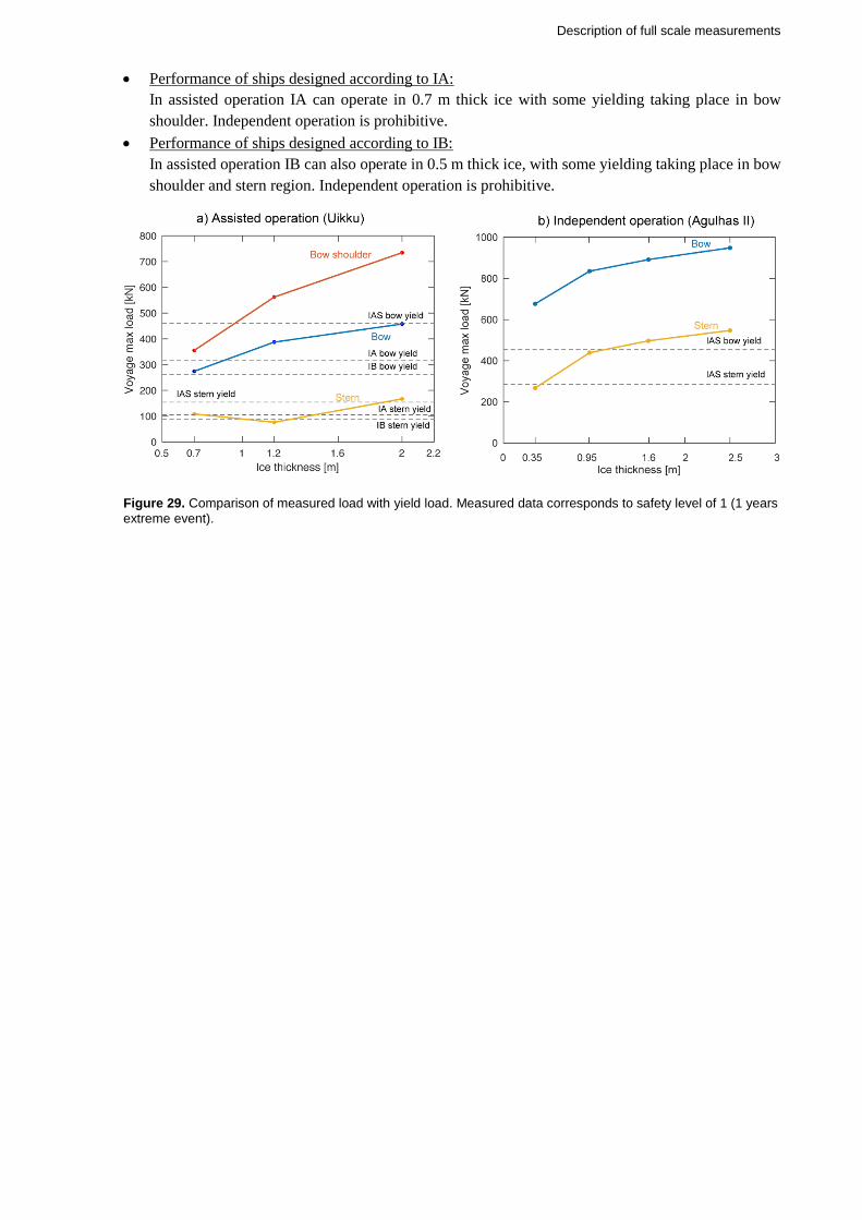
Description of full scale measurements
Performance of ships designed according to IA:
In assisted operation IA can operate in 0.7 m thick ice with some yielding taking place in bow
shoulder. Independent operation is prohibitive.
Performance of ships designed according to IB:
In assisted operation IB can also operate in 0.5 m thick ice, with some yielding taking place in bow
shoulder and stern region. Independent operation is prohibitive.
Figure 29. Comparison of measured load with yield load. Measured data corresponds to safety level of 1 (1 years
extreme event).
8. Comparison of results with preliminary assessment in Polar Code
IMO has adopted the International Code for Ships Operating in Polar Waters (Polar Code) and
related amendments both to the International Convention for the Safety of Life at Sea (SOLAS)
and the International Convention for the Prevention of Pollution from Ships (MARPOL) to
make the Polar Code mandatory. One of the aspects of the Polar Code addresses the operational
limitations of ships of different categories (A, B and C) according to ice conditions. The ap-
proach for evaluating the ice conditions and setting limitations for ships assigned an ice class
is called POLARIS – Polar Operational Limit Assessment Risk Indexing System, details of
which are given in MSC.1/Circ.1519 (2016). Therein the ice classes are associated with the
limiting ice thickness by combining the experience from three existing approaches used in ice-
covered waters: the Canadian Arctic, the Baltic (Finnish/Swedish), and the Russian Northern
Sea Route systems. The assessment given in MSC 94 (2014) categorizes ships designed accord-
ing to the Finnish Swedish Ice Class Rules (FSICR) for different operational conditions. Here,
the validity of this preliminary assessment is discussed in the light of the results presented in
the previous Section.
8.1 Limitations
Before discussing the validity of the preliminary assessment, it is important to highlight the
limitations of the present findings. First, the measurement data is never as exhaustive as it could
be – this applies to the data used herein as well. Agulhas II data is based on one voyage making
the long-term predictions less reliable. During the measurement period Uikku operated 2 weeks
in rather extreme conditions that could lead to higher load levels than usually experienced.
Moreover, the amount of data is scarce for Uikku as the voyage was only 2 weeks long. In
addition, the loading data was gathered only in 20 minute intervals – decreasing the interval
would have doubled the amount of data.
Furthermore, both ships have an icebreaking hull form that means that the ice breaking pro-
cess is more efficient and experienced loads potentially lower compared to hull forms, which
are optimized for sailing in open water, e.g. hull forms with a bulbous bow. The design require-
ments of the FSICR, however, do not take the hull form into account and thus, in the analyses,
structures were assumed vertical.
Related to numerical simulations there are two major uncertainties: 1) the neglection of brack-
ets in FE models and 2) the assumed non-uniform pressure profile applied to the structure. The
former presumably makes the structures slightly weaker, so there is additional implicit safety
margin built into the analysis results. The latter, as demonstrated in Section 4, reduces stiffness
compared with the design approach of the FSICR. In effect, the combination of these two as-
sumptions can potentially cancel each other as modelled brackets would have reduced defor-
mations, while non-uniform pressure patch increased deformations.
8.2 Assisted operation
In POLARIS system, the operational restrictions are based on the definitions given in the Ice
Nomenclature of WMO. Safe operational ice conditions for assisted operation in first-year ice
are given in Table 6 together with the assessment made in this study (safety level of 0.1). Com-
parison reveals that the preliminary assessment is more conservative, especially for higher ice

Conclusions
classes. For IB ice class, the current extensive simulation based assessment gives only a 10 cm
thinnerlimiting ice thickness value than the preliminary assessment.
Table 6. Comparison between the preliminary assessment from POLARIS and the assessment done in this study for safe operation of ships in first-year winter ice regime for the Finnish-Swedish ice classes, when icebreaker assistance is provided or the ice concentration is less than 100%. SLS means the serviceability limit state.
8.3 Independent operation
According to the POLARIS system the Polar Ship Certificate given for independently operating
ships in first-year ice imposes operational limitations only based on ice thickness, and not by
ice concentration, see Appendix A.
Current results are consistent with the preliminary assessment made in POLARIS for ice clas-
ses IA Super and IA, but operation by IB class vessel is prohibitive, see Table 7.
Table 7. Comparison between th preliminary assessment from POLARIS and the assessment done in this study for safe operation of ships in first-year winter ice regime for the Finnish-Swedish ice classes during independent operation.
9. Conclusions
This study had two important objectives: first, analyse the limit states of frame and plating and
second, assess the validity of the preliminary assessment of the operational restrictions for ships
ice-strengthened in accordance with different Finnish-Swedish Ice Classes.
The limit state analysis showed that boundary conditions as well as load application has an
important consequence on the load levels. Load applied according to the FSICR via uniform
pressure patch resulted in the lowest frame stiffness, but the corresponding line load was sig-
nificantly higher, and less consistent with measured line load values than some of the alternative
load patches used. Therefore, to manifest large deformations on structures, but keep the com-
pliance with measured line load values, a non-uniform pressure patch was used to determine
the permanent deformations in the structure.
The load height, i.e. line-like contact as opposed to current design approach, was shown to
significantly reduce the capacity of a single frame while the effect on total structural stiffness
was insignificant. This leads to two conclusions. First, as the effect was so strong, the results
would have been much more conservative than presented in the previous section. Therefore, to
keep compliance with present design approach, we did not use this approach in evaluating the
Ice class WMO description of the ice regime Thickness of ice floes, hi SLS YieldIA Super Medium first-year ice hi up to about 100 cm 200 cm 100 cm
IA Medium first-year ice hi up to about 80 cm 120 cm 70 cm (some yielding)
IB Thin first-year ice hi up to about 60 cm 100 cm 50 cm (some yielding)
IC Thin first-year ice hi up to about 40 cm - -
POLARIS assessment (Polar Code) Current assessment [cm]
Thicknessoficefloes,hi
Iceconcentration,Ciupto100%
IASuper Mediumfirst-yearice hiuptoabout80cm 100cm
IA Mediumfirst-yearice hiuptoabout70cm 50cm
IB Thinfirst-yearice hiuptoabout50cm prohibitive
IC Thinfirst-yearice hiuptoabout30cm -
Iceclass WMOdescriptionoftheiceregime Currentassessment[cm]
Polarisassessment

response of frames. Second, it also leads us to think how the total load should be interpreted in
terms of frame response. Here, the load on single frame was obtained by integrating the applied
load over the frame spacing. In contrast, experimental values are obtained via the shear gauges
attached on the both ends of the frame, and by the measured shear strain difference. Future
investigations should consider this aspect when presenting “load on frame”.
Consequently, the proposed NUPP loading scenario was used with a load height consistent
with the present design rules to determine the serviceability limit state (SLS) of two ships de-
signed according to three ice classes: IA Super, IA and IB. The permanent set limit of s/12
given by DNV was used as a SLS and the load causing this was defined using non-linear FE
simulations.
The two ships were chosen as the long-term measurement data was available for these ships
and the ships represented two alternative operating regimes: independent operation (SA Agul-
has II) and operation assisted with icebreakers (Uikku). Therefore, we could compare the most
probable loads experienced by ships estimated by using long-term measured data with our anal-
ysis results. The probability of the load was associated with safety factor of 0.1 and 1. The
safety factor of 0.1 is consistent with SLS design standard to ensure functionality under any 10-
year ice event and safety factor of 1 ensures functionality under one year extreme event, which
according to the FSICR is the state of yielding.
This comparison reveals the maximum ice thickness for assisted and independent operation
for different ice classes, or in other words, defines the operational limitiations for ice strength-
ened ships designed according to the FSICR. Similar preliminary assessment of limiting ice
thicknesses for safe operation are given in the Polar Code, but without supporting FE analysis.
When serviceability is considered as a limiting condition for safe operation, results encourag-
ingly show that the present designs are safer than assumed in the Polar Code when operating
under icebreaker assistance or when ice concentration is less than 100%. This extra safety de-
pends on the ice class, with IA Super showing the largest safety margin. When conservatively
associating yield with the safe operation, the limiting ice thicknesses provided by POLARIS
correlates well with the present findings. Still, it is important to highlight the fact that Uikku
has multifunctional icebreaking hull form which possibly decreases the measured loads. Nev-
ertheless, results can be generalized to blunt hull forms as the largest measured loads are meas-
ured on the shoulder area, where the frame angle is not substantially different between a multi-
functional icebreaking hull and a blunt hull. Independent operation however, is according to
our assessment quite consistent with Polar Code assessment when the permanent deflection
limit state of s/12 is used.
References Abraham, J., 2008. PLASTIC RESPONSE OF SHIP STRUCTURE SUBJECTED TO ICE LOADING.
Master thesis, Memorial University of Newfoundland.
Abraham, J., Daley, C.G., 2009. Load Sharing in a Grillage Subject to Ice Loading, Presented at the
RINA International Conference on Ship and Offshore Technology, Ice Class Vessels. Busan, Ko-
rea., pp. 1–5.
ABS 2014. Guidance notes on ice class. American Bureau of Shipping.
Daley, C.G., 2002. Derivation of plastic framing requirements for polar ships. Mar. Struct. 15, 543–
559.
Daley, C.G., 2007. Reanalysis of ice pressure-area relationships. Marine Technology 44, 234–244.

References
Erceg, B., Taylor, R. & Ehlers, S., 2014. A Response Comparison of a Stiffened Panel Subjected to Rule-
Based and Measured Ice Loads. In: Proceedings of the ASME 2014 33rd International Confer-
ence on Ocean, Offshore and Arctic Engineering, OMAE2014 June 8-13, 2014, San Francisco,
California, USA.
Hogström, P., Ringsberg, J.W., Johnson, E., 2009. An experimental and numerical study of the effects
of length scale and strain state on the necking and fracture behaviours in sheet metals. Int. J.
Impact Eng. 36, 1194–1203. doi:10.1016/j.ijimpeng.2009.05.005
IACS, 2011. Unified Requirements for Polar Ships: I2 - structural requirements for Polar Class ships.
International Association of Classification Societies.
ISO 19906:2010, Petroleum and natural gas industries - Arctic offshore structures. Section 7: Reliabil-
ity and limit state design.
ISSC 2015, 19th INTERNATIONAL SHIP AND OFFSHORE STRUCTURES CONGRESS, Committee
V.6 Arctic Technology, Edited by Soares, C.G. & Garbatov,Y. CRC Press.
Jordaan, I.J., Singh, S.K., 1994. Compressive ice failure: critical zones of high pressure. IAHR Ice Sym-
posium, Trondheim, Norway, pp. 505–514.
Kotisalo, K., and Kujala, P. 1999. Ice load measurements onboard MT Uikku during the ARCDEV voy-
age, 2013. POAC’99, proceedings, Vol 3, Espoo, pp. 974-987. Kujala, P. and Vuorio, J. 1986. Results and statistical analysis of ice load measurements on board ice-
breaker Sisu in winters 1979 to 1985,” Finnish Board of Navigation, Winter navigation Research
Board, Research report No 43, 1986.
Kurmiste, A. (2016). “Analysis of structural safety of ice-going vessels in the Arctic and Antarctic”.
Master thesis. Aalto University, School of Engineering.
Lepik, K., Peetsalu, J., Viljakainen, S., and Voog, V. 2010. Allowable plate deflections according to
DNV.
Lyngra, N.H.L., 2014. Analysis of Ice-Induced Damages to a Cargo Carrier and Implications wrt. Rule
Requirements. Master thesis. Norwegian university of Science and Technology, NTNU.
MSC.1/Circ.1519 (2016). Guidance on Methodologies for assessing Operational Capabilities and Limi-
tations in Ice. International Maritime Organization, 2016.
MSC 94/INF.13 (2014). Technical background to POLARIS. Submitted by Canada, Finland, Sweden
and the International Association of Classification Societies (IACS). 94th session of the Maritime
Safety Committee of IMO, 2014.
Quinton, B.W.T., Daley, C.G., Gagnon, R.E., 2010. Effect of Moving Ice Loads on the Plastic Capacity
of a Ship's Structure. In: International Conference and Exhibition on Performance of Ships and
Structures in Ice (ICETECH 2010), September 20-23, Anchorage, Alaska.
Quinton, B.W.T., Daley, C.G., Gagnon, R.E., 2012. Realistic Moving Ice Loads And Ship Structural Re-
sponse, in: Proceedings of the Twenty-second (2012) International Offshore and Polar Engi-
neering Conference Rhodes, Greece, June 17-22.
Riska, K. and Kämäräinen, J. 2012. Comparison of Finnish-Swedish and IACS Ice Class Rules. The
Royal Institution of Naval Architects. The Ice Class Ships, 4-5 July 2012, London, UK.
Riska, K., Kämäräinen, J., 2011. A review of ice loading and the evolution of the finnish-swedish ice
class rules. Proceedings of the SNAME Annual Meeting.
Suominen, M, and Kujala, P. The Measured Line Load As A Function Of The Load Length In The Ant-
arctic Waters. Proceedings of the 23rd International Conference on Port and Ocean Engineering
under Arctic Conditions. 2015.
Suominen, M., et al. 2013. FULL-SCALE MEASUREMENTS ON BOARD PSRV S.A. AGULHAS II IN
THE BALTIC SEA 1–12. POAC’13, proceedings.
Suominen, M., Kujala, P. 2015. THE MEASURED LINE LOAD AS A FUNCTION OF THE LOAD
LENGTH IN THE ANTARCTIC WATERS, in:. Presented at the Proceedings of the 23rd Interna-
tional Conference on Port and Ocean Engineering under Arctic Conditions, POAC’15.
Suominen, M., Kujala, P., Kotilainen, M., 2015. THE ENCOUNTERED EXTREME EVENTS AND PRE-
DICTED MAXIMUM ICE-INDUCED LOADS ON THE SHIP HULL IN THE SOUTHERN

OCEAN , in:. Presented at the Proceedings of the ASME th International Conference on Ocean,
Offshore and Arctic Engineering OMAE May 31-June 5, St. Johns, Newfoundland, Canada.

Appendix A. Excerpt from MSC 94/INF.13 (2014).
Appendix A. Excerpt from MSC 94/INF.13 (2014).