1

OpenModelica Users Guide

Version 2009-11-09for OpenModelica 1.5

November 2009

Peter Fritzson Adrian Pop, Peter Aronsson,

David Akhvlediani, Bernhard Bachmann, Vasile Baluta, Simon Björklén, Mikael Blom, Willi Braun, David Broman, Stefan Brus,

Francesco Casella, Filippo Donida, Henrik Eriksson, Anders Fernström, Jens Frenkel, Pavel Grozman, Daniel Hedberg, Michael Hanke, Alf Isaksson, Kim

Jansson, Daniel Kanth, Tommi Karhela, Joel Klinghed, Juha Kortelainen, Alexey Lebedev, Magnus Leksell, Oliver Lenord, Håkan Lundvall, Henrik

Magnusson, Eric Meyers, Hannu Niemistö, Kristoffer Norling, Atanas Pavlov, Pavol Privitzer, Per Sahlin, Wladimir Schamai, Gerhard Schmitz, Klas Sjöholm, Martin Sjölund, Kristian Stavåker, Mohsen Torabzadeh-Tari, Niklas Worschech,

Robert Wotzlaw, Björn Zackrisson

Copyright by:

Linköping University, SwedenDepartment of Computer and Information Science

Supported by:

2

Open Source Modelica Consortium

3

Copyright © 1998-2009, Linköpings universitet, Department of Computer and Information Science. SE-58183 Linköping, Sweden

All rights reserved.

THIS PROGRAM IS PROVIDED UNDER THE TERMS OF THIS OSMC PUBLIC LICENSE (OSMC-PL). ANY USE, REPRODUCTION OR DISTRIBUTION OF THIS PROGRAM CONSTITUTES RECIPIENT'S ACCEPTANCE OF THE OSMC PUBLIC LICENSE.

The OpenModelica software and the OSMC (Open Source Modelica Consortium) Public License (OSMC-PL) are obtained from Linköpings universitet, either from the above address, from the URL: http://www.ida.liu.se/projects/OpenModelica, and in the OpenModelica distribution.

This program is distributed WITHOUT ANY WARRANTY; without even the implied warranty of MERCHANTABILITY or FITNESS FOR A PARTICULAR PURPOSE, EXCEPT AS EXPRESSLY SET FORTH IN THE BY RECIPIENT SELECTED SUBSIDIARY LICENSE CONDITIONS OF OSMC-PL.

See the full OSMC Public License conditions for more details.

This document is part of OpenModelica: www.openmodelica.orgContact: OpenModelica@ida.liu.se

Modelica® is a registered trademark of Modelica Association.

MathModelica® is a registered trademark of MathCore Engineering AB.

Mathematica® is a registered trademark of Wolfram Research Inc.

4

Table of Contents

Table of Contents..................................................................................................................................4

Preface 8

Chapter 1

Introduction 10

1.1 System Overview..........................................................................................................................111.1.1 Implementation Status...........................................................................................................12

1.2 Interactive Session with Examples................................................................................................131.2.1 Starting the Interactive Session..............................................................................................131.2.2 Trying the Bubblesort Function.............................................................................................131.2.3 Trying the system and cd Commands....................................................................................141.2.4 Modelica Library and DCMotor Model.................................................................................151.2.5 The val() function..................................................................................................................171.2.6 BouncingBall and Switch Models..........................................................................................171.2.7 Clear All Models....................................................................................................................191.2.8 VanDerPol Model and Parametric Plot..................................................................................201.2.9 Scripting with For-Loops, While-Loops, and If-Statements..................................................201.2.10 Variables, Functions, and Types of Variables......................................................................221.2.11 Using External Functions.....................................................................................................221.2.12 Calling the Model Query and Manipulation API.................................................................231.2.13 Quit OpenModelica..............................................................................................................241.2.14 Dump XML Representation.................................................................................................241.2.15 Dump Matlab Representation..............................................................................................24

1.3 Summary of Commands for the Interactive Session Handler........................................................251.4 References.....................................................................................................................................26

Chapter 2

Using the Graphical Model Editor.......................................................................................................27

2.1 Getting Started...............................................................................................................................272.2 Creating a new project...................................................................................................................28

2D Plotting and 3D Animation..............................................................................................................32

2.3 Enhanced Qt-based 2D Plot Functionality....................................................................................322.4 Simple 2D Plot..............................................................................................................................33

2.4.1 All Plot Functions and their Options......................................................................................36

5

2.4.2 Zooming.................................................................................................................................372.4.3 Plotting all variables of a model............................................................................................382.4.4 Plotting During Simulation....................................................................................................392.4.5 Programmable Drawing of 2D Graphics................................................................................402.4.6 Plotting of table data..............................................................................................................41

2.5 Java-based PtPlot 2D plotting.......................................................................................................422.6 3D Animation................................................................................................................................42

2.6.1 Object Based Visualization....................................................................................................432.6.2 BouncingBall.........................................................................................................................43

2.6.2.1 Adding Visualization......................................................................................................442.6.2.2 Running the Simulation and Starting Visualization.......................................................44

2.6.3 Pendulum 3D Example..........................................................................................................452.6.3.1 Adding the Visualization................................................................................................46

2.7 References.....................................................................................................................................47

Chapter 3

OMNotebook with DrModelica............................................................................................................49

3.1 Interactive Notebooks with Literate Programming.......................................................................493.1.1 Mathematica Notebooks........................................................................................................493.1.2 OMNotebook.........................................................................................................................49

3.2 The DrModelica Tutoring System – an Application of OMNotebook..........................................503.3 OpenModelica Notebook Commands...........................................................................................55

3.3.1 Cells 563.3.2 Cursors...................................................................................................................................56

3.4 Selection of Text or Cells..............................................................................................................563.4.1 File Menu...............................................................................................................................573.4.2 Edit Menu..............................................................................................................................573.4.3 Cell Menu..............................................................................................................................583.4.4 Format Menu.........................................................................................................................583.4.5 Insert Menu............................................................................................................................593.4.6 Window Menu.......................................................................................................................593.4.7 Help Menu.............................................................................................................................593.4.8 Additional Features................................................................................................................60

3.5 References.....................................................................................................................................61

Chapter 4

MDT – The OpenModelica Development Tooling Eclipse Plugin.....................................................62

4.1 Introduction...................................................................................................................................624.2 Installation.....................................................................................................................................624.3 Getting Started...............................................................................................................................63

4.3.1 Configuring the OpenModelica Compiler.............................................................................634.3.2 Using the Modelica Perspective.............................................................................................634.3.3 Selecting a Workspace Folder................................................................................................634.3.4 Creating one or more Modelica Projects................................................................................644.3.5 Building and Running a Project.............................................................................................654.3.6 Switching to Another Perspective..........................................................................................664.3.7 Creating a Package.................................................................................................................674.3.8 Creating a Class.....................................................................................................................674.3.9 Syntax Checking....................................................................................................................684.3.10 Automatic Indentation Support............................................................................................694.3.11 Code Completion.................................................................................................................70

6

4.3.12 Code Assistance on Identifiers when Hovering ..................................................................714.3.13 Go to Definition Support.....................................................................................................714.3.14 Code Assistance on Writing Records...................................................................................714.3.15 Using the MDT Console for Plotting...................................................................................73

Chapter 5

Modelica Algorithmic Subset Debugger..............................................................................................74

5.1 The Eclipse-based debugging environment...................................................................................745.2 Starting the Modelica Debugging Perspective...............................................................................75

5.2.1 Setting the debug configuration.............................................................................................755.2.2 Setting/Deleting Breakpoints.................................................................................................775.2.3 Starting the debugging session and enabling the debug perspective......................................78

5.3 The Debugging Perspective...........................................................................................................79

Chapter 6

Interoperability – C, Java, and Python................................................................................................80

6.1 Calling External C functions.........................................................................................................806.2 Calling External Java Functions....................................................................................................816.3 Python Interoperability..................................................................................................................82

Chapter 7

Frequently Asked Questions (FAQ).....................................................................................................84

7.1 OpenModelica General..................................................................................................................847.2 OMNotebook.................................................................................................................................847.3 OMDev - OpenModelica Development Environment...................................................................85

Appendix A

Major OpenModelica Releases.............................................................................................................86

A.1 OpenModelica 1.5, November 2009.............................................................................................86A.1.1 OpenModelica Compiler (OMC)..........................................................................................86

A.2 OpenModelica 1.4.5, January 2009..............................................................................................86A.2.1 OpenModelica Compiler (OMC)..........................................................................................86A.2.2 OpenModelica Notebook (OMNotebook)............................................................................87A.2.3 OpenModelica Shell (OMShell)...........................................................................................87A.2.4 OpenModelica Eclipse Plug-in (MDT).................................................................................87A.2.5 OpenModelica Development Environment (OMDev) .........................................................87

A.3 OpenModelica 1.4.4, Feb 2008.....................................................................................................87A.3.1 OpenModelica Compiler (OMC)..........................................................................................87A.3.2 OpenModelica Notebook (OMNotebook)............................................................................87A.3.3 OpenModelica Shell (OMShell)...........................................................................................88A.3.4 OpenModelica Eclipse Plug-in (MDT).................................................................................88A.3.5 OpenModelica Development Environment (OMDev) .........................................................88

A.4 OpenModelica 1.4.3, June 2007...................................................................................................88A.4.1 OpenModelica Compiler (OMC)..........................................................................................88A.4.2 OpenModelica Notebook (OMNotebook)............................................................................89A.4.3 OpenModelica Shell (OMShell)...........................................................................................89A.4.4 OpenModelica Eclipse Plug-in (MDT).................................................................................89A.4.5 OpenModelica Development Environment (OMDev) .........................................................89

A.5 OpenModelica 1.4.2, October 2006..............................................................................................89A.5.1 OpenModelica Compiler (OMC)..........................................................................................89

7

A.5.2 OpenModelica Notebook (OMNotebook)............................................................................89A.5.3 OpenModelica Eclipse Plug-in (MDT).................................................................................90A.5.4 OpenModelica Development Environment (OMDev) .........................................................90

A.6 OpenModelica 1.4.1, June 2006...................................................................................................90A.6.1 OpenModelica Compiler (OMC)..........................................................................................90A.6.2 OpenModelica Eclipse Plug-in (MDT).................................................................................90A.6.3 OpenModelica Development Environment (OMDev) .........................................................90

A.7 OpenModelica 1.4.0, May 2006...................................................................................................90A.7.1 OpenModelica Compiler (OMC)..........................................................................................90A.7.2 OpenModelica Shell (OMShell)...........................................................................................91A.7.3 OpenModelica Notebook (OMNotebook)............................................................................91A.7.4 OpenModelica Eclipse Plug-in (MDT).................................................................................91A.7.5 OpenModelica Development Environment (OMDev)..........................................................91

A.8 OpenModelica 1.3.1, November 2005..........................................................................................91A.8.1 OpenModelica Compiler (OMC)..........................................................................................91A.8.2 OpenModelica Shell (OMShell)...........................................................................................92A.8.3 OpenModelica Notebook (OMNotebook)............................................................................92A.8.4 OpenModelica Eclipse Plug-in (MDT).................................................................................92A.8.5 OpenModelica Development Environment (OMDev)..........................................................92

Appendix B

Contributors to OpenModelica.............................................................................................................93

B.1 OpenModelica Contributors 2009.................................................................................................93B.2 OpenModelica Contributors 2008.................................................................................................94B.3 OpenModelica Contributors 2007.................................................................................................94B.4 OpenModelica Contributors 2006.................................................................................................95B.5 OpenModelica Contributors 2005.................................................................................................95B.6 OpenModelica Contributors 2004.................................................................................................95B.7 OpenModelica Contributors 2003.................................................................................................96B.8 OpenModelica Contributors 2002.................................................................................................96B.9 OpenModelica Contributors 2001.................................................................................................96B.10 OpenModelica Contributors 2000...............................................................................................96B.11 OpenModelica Contributors 1999...............................................................................................96B.12 OpenModelica Contributors 1998...............................................................................................97 Index 98

Preface This users guide provides documentation and examples on how to use the OpenModelica system, both for the Modelica beginners and advanced users.

Chapter 1

Introduction

The OpenModelica system described in this document has both short-term and long-term goals:

The short-term goal is to develop an efficient interactive computational environment for the Modelica language, as well as a rather complete implementation of the language. It turns out that with support of appropriate tools and libraries, Modelica is very well suited as a computational language for development and execution of both low level and high level numerical algorithms, e.g. for control system design, solving nonlinear equation systems, or to develop optimization algorithms that are applied to complex applications.

The longer-term goal is to have a complete reference implementation of the Modelica language, including simulation of equation based models and additional facilities in the programming environment, as well as convenient facilities for research and experimentation in language design or other research activities. However, our goal is not to reach the level of performance and quality provided by current commercial Modelica environments that can handle large models requiring advanced analysis and optimization by the Modelica compiler.

The long-term research related goals and issues of the OpenModelica open source implementation of a Modelica environment include but are not limited to the following:

Development of a complete formal specification of Modelica, including both static and dynamic semantics. Such a specification can be used to assist current and future Modelica implementers by providing a semantic reference, as a kind of reference implementation.

Language design, e.g. to further extend the scope of the language, e.g. for use in diagnosis, structural analysis, system identification, etc., as well as modeling problems that require extensions such as partial differential equations, enlarged scope for discrete modeling and simulation, etc.

Language design to improve abstract properties such as expressiveness, orthogonality, declarativity, reuse, configurability, architectural properties, etc.

Improved implementation techniques, e.g. to enhance the performance of compiled Modelica code by generating code for parallel hardware.

Improved debugging support for equation based languages such as Modelica, to make them even easier to use.

Easy-to-use specialized high-level (graphical) user interfaces for certain application domains. Visualization and animation techniques for interpretation and presentation of results. Application usage and model library development by researchers in various application areas.

The OpenModelica environment provides a test bench for language design ideas that, if successful, can be submitted to the Modelica Association for consideration regarding possible inclusion in the official Modelica standard.

The current version of the OpenModelica environment allows most of the expression, algorithm, and function parts of Modelica to be executed interactively, as well as equation models and Modelica functions to be compiled into efficient C code. The generated C code is combined with a library of utility functions, a run-time library, and a numerical DAE solver. An external function library interfacing a LAPACK subset and other basic algorithms is under development.

1.1 System OverviewThe OpenModelica environment consists of several interconnected subsystems, as depicted in Figure 1-1 below.

Figure 1-1. The architecture of the OpenModelica environment. Arrows denote data and control flow. The interactive session handler receives commands and shows results from evaluating commands and expressions that are translated and executed. Several subsystems provide different forms of browsing and textual editing of Modelica code. The debugger currently provides debugging of an extended algorithmic subset of Modelica. The graphical model editor is not really part of OpenModelica but integrated into the system and available from MathCore without cost for academic usage.

The following subsystems are currently integrated in the OpenModelica environment:

An interactive session handler, that parses and interprets commands and Modelica expressions for evaluation, simulation, plotting, etc. The session handler also contains simple history facilities, and completion of file names and certain identifiers in commands.

A Modelica compiler subsystem, translating Modelica to C code, with a symbol table containing definitions of classes, functions, and variables. Such definitions can be predefined, user-defined, or obtained from libraries. The compiler also includes a Modelica interpreter for interactive usage and constant expression evaluation. The subsystem also includes facilities for building simulation executables linked with selected numerical ODE or DAE solvers.

An execution and run-time module. This module currently executes compiled binary code from translated expressions and functions, as well as simulation code from equation based models, linked

with numerical solvers. In the near future event handling facilities will be included for the discrete and hybrid parts of the Modelica language.

Emacs textual model editor/browser. In principle any text editor could be used. We have so far primarily employed Gnu Emacs, which has the advantage of being programmable for future extensions. A Gnu Emacs mode for Modelica has previously been developed. The Emacs mode hides Modelica graphical annotations during editing, which otherwise clutters the code and makes it hard to read. A speedbar browser menu allows to browse a Modelica file hierarchy, and among the class and type definitions in those files.

Eclipse plugin editor/browser. The Eclipse plugin called MDT (Modelica Development Tooling) provides file and class hierarchy browsing and text editing capabilities, rather analogous to previously described Emacs editor/browser. Some syntax highlighting facilities are also included. The Eclipse framework has the advantage of making it easier to add future extensions such as refactoring and cross referencing support.

OMNotebook DrModelica model editor. This subsystem provides a lightweight notebook editor, compared to the more advanced Mathematica notebooks available in MathModelica. This basic functionality still allows essentially the whole DrModelica tutorial to be handled. Hierarchical text documents with chapters and sections can be represented and edited, including basic formatting. Cells can contain ordinary text or Modelica models and expressions, which can be evaluated and simulated. However, no mathematical typesetting or graphic plotting facilities are yet available in the cells of this notebook editor.

Graphical model editor/browser. This is a graphical connection editor, for component based model design by connecting instances of Modelica classes, and browsing Modelica model libraries for reading and picking component models. The graphical model editor is not really part of OpenModelica but integrated into the system and provided by MathCore without cost for academic usage. The graphical model editor also includes a textual editor for editing model class definitions, and a window for interactive Modelica command evaluation.

Modelica debugger. The current implementation of debugger provides debugging for an extended algorithmic subset of Modelica, excluding equation-based models and some other features, but including some meta-programming and model transformation extensions to Modelica. This is conventional full-feature debugger, using Emacs for displaying the source code during stepping, setting breakpoints, etc. Various back-trace and inspection commands are available. The debugger also includes a data-view browser for browsing hierarchical data such as tree- or list structures in extended Modelica.

1.1.1 Implementation StatusIn the current OpenModelica implementation version 1.5 (November 2009), not all subsystems are yet integrated as well as is indicated in Figure 1-1. Currently there are two versions of the Modelica compiler, one which supports most of standard Modelica including simulation, and is connected to the interactive session handler, the notebook editor, and the graphic model editor, and another meta-programming Modelica compiler version (called MetaModelica compiler) which is integrated with the debugger and Eclipse, supports meta-programming Modelica extensions, but does not allow equation-based modeling and simulation. Those two versions have in OpenModelica 1.5 merged into a single Modelica compiler version. All MetaModelica constructs now work inside OpenModelica, but more bugfixing and performance tuning remains.

1.2 Interactive Session with ExamplesThe following is an interactive session using the interactive session handler in the OpenModelica environment, called OMShell – the OpenModelica Shell). Most of these examples are also available in the OpenModelica notebook UsersGuideExamples.onb in the testmodels directory, see also Chapter 3.

1.2.1 Starting the Interactive SessionThe Windows version which at installation is made available in the start menu as OpenModelica->OpenModelica Shell which responds with an interaction window:

We enter an assignment of a vector expression, created by the range construction expression 1:12, to be stored in the variable x. The value of the expression is returned.>> x := 1:12 {1, 2, 3, 4, 5, 6, 7, 8, 9, 10, 11, 12}

1.2.2 Trying the Bubblesort FunctionLoad the function bubblesort, either by using the pull-down menu File->Load Model, or by explicitly giving the command:>> loadFile("C:/OpenModelica1.5/testmodels/bubblesort.mo")

true

The function bubblesort is called below to sort the vector x in descending order. The sorted result is returned together with its type. Note that the result vector is of type Real[:], instantiated as Real[12], since this is the declared type of the function result. The input Integer vector was automatically converted to a Real vector according to the Modelica type coercion rules. The function is automatically compiled when called if this has not been done before.>> bubblesort(x){12.0,11.0,10.0,9.0,8.0,7.0,6.0,5.0,4.0,3.0,2.0,1.0}

Another call:>> bubblesort({4,6,2,5,8}){8.0,6.0,5.0,4.0,2.0}

It is also possible to give operating system commands via the system utility function. A command is provided as a string argument. The example below shows the system utility applied to the UNIX command cat, which here outputs the contents of the file bubblesort.mo to the output stream. However, the cat command does not boldface Modelica keywords – this improvement has been done by hand for readability.>> cd("C:/OpenModelica1.5/testmodels")>> system("cat bubblesort.mo")

function bubblesort input Real[:] x; output Real[size(x,1)] y;protected Real t;algorithm y := x; for i in 1:size(x,1) loop for j in 1:size(x,1) loop if y[i] > y[j] then t := y[i]; y[i] := y[j]; y[j] := t; end if; end for; end for;end bubblesort;

1.2.3 Trying the system and cd CommandsNote: Under Windows the output emitted into stdout by system commands is put into the winmosh console windows, not into the winmosh interaction windows. Thus the text emitted by the above cat command would not be returned. Only a success code (0 = success, 1 = failure) is returned to the winmosh window. For example: >> system("dir")0

>> system("Non-existing command")1

Another built-in command is cd, the change current directory command. The resulting current directory is returned as a string.>> cd()"C:\OpenModelica1.5\testmodels"

>> cd("..")"C:\OpenModelica1.5"

>> cd("C:\\OpenModelica1.5\\testmodels")"C:\OpenModelica1.5\testmodels"

1.2.4 Modelica Library and DCMotor ModelWe load a model, here the whole Modelica standard library, which also can be done through the File->Load Modelica Library menu item:>> loadModel(Modelica)true

We also load a file containing the dcmotor model:>> loadFile("C:/OpenModelica1.5/testmodels/dcmotor.mo")true

It is simulated:>> simulate(dcmotor,startTime=0.0,stopTime=10.0)

record resultFile = "dcmotor_res.plt"end record

We list the source code of the model:>> list(dcmotor)

"model dcmotor Modelica.Electrical.Analog.Basic.Resistor r1(R=10); Modelica.Electrical.Analog.Basic.Inductor i1; Modelica.Electrical.Analog.Basic.EMF emf1; Modelica.Mechanics.Rotational.Inertia load; Modelica.Electrical.Analog.Basic.Ground g; Modelica.Electrical.Analog.Sources.ConstantVoltage v;

equation connect(v.p,r1.p); connect(v.n,g.p); connect(r1.n,i1.p); connect(i1.n,emf1.p); connect(emf1.n,g.p); connect(emf1.flange_b,load.flange_a);end dcmotor;"

We test code instantiation of the model to flat code:>> instantiateModel(dcmotor)

"fclass dcmotorReal r1.v "Voltage drop between the two pins (= p.v - n.v)";Real r1.i "Current flowing from pin p to pin n";Real r1.p.v "Potential at the pin";Real r1.p.i "Current flowing into the pin";Real r1.n.v "Potential at the pin";Real r1.n.i "Current flowing into the pin";parameter Real r1.R = 10 "Resistance";Real i1.v "Voltage drop between the two pins (= p.v - n.v)";

Real i1.i "Current flowing from pin p to pin n";Real i1.p.v "Potential at the pin";Real i1.p.i "Current flowing into the pin";Real i1.n.v "Potential at the pin";Real i1.n.i "Current flowing into the pin";parameter Real i1.L = 1 "Inductance";parameter Real emf1.k = 1 "Transformation coefficient";Real emf1.v "Voltage drop between the two pins";Real emf1.i "Current flowing from positive to negative pin";Real emf1.w "Angular velocity of flange_b";Real emf1.p.v "Potential at the pin";Real emf1.p.i "Current flowing into the pin";Real emf1.n.v "Potential at the pin";Real emf1.n.i "Current flowing into the pin";Real emf1.flange_b.phi "Absolute rotation angle of flange";Real emf1.flange_b.tau "Cut torque in the flange";Real load.phi "Absolute rotation angle of component (= flange_a.phi = flange_b.phi)";Real load.flange_a.phi "Absolute rotation angle of flange";Real load.flange_a.tau "Cut torque in the flange";Real load.flange_b.phi "Absolute rotation angle of flange";Real load.flange_b.tau "Cut torque in the flange";parameter Real load.J = 1 "Moment of inertia";Real load.w "Absolute angular velocity of component";Real load.a "Absolute angular acceleration of component";Real g.p.v "Potential at the pin";Real g.p.i "Current flowing into the pin";Real v.v "Voltage drop between the two pins (= p.v - n.v)";Real v.i "Current flowing from pin p to pin n";Real v.p.v "Potential at the pin";Real v.p.i "Current flowing into the pin";Real v.n.v "Potential at the pin";Real v.n.i "Current flowing into the pin";parameter Real v.V = 1 "Value of constant voltage";equation r1.R * r1.i = r1.v; r1.v = r1.p.v - r1.n.v; 0.0 = r1.p.i + r1.n.i; r1.i = r1.p.i; i1.L * der(i1.i) = i1.v; i1.v = i1.p.v - i1.n.v; 0.0 = i1.p.i + i1.n.i; i1.i = i1.p.i; emf1.v = emf1.p.v - emf1.n.v; 0.0 = emf1.p.i + emf1.n.i; emf1.i = emf1.p.i; emf1.w = der(emf1.flange_b.phi); emf1.k * emf1.w = emf1.v; emf1.flange_b.tau = -(emf1.k * emf1.i); load.w = der(load.phi); load.a = der(load.w); load.J * load.a = load.flange_a.tau + load.flange_b.tau; load.flange_a.phi = load.phi; load.flange_b.phi = load.phi; g.p.v = 0.0; v.v = v.V; v.v = v.p.v - v.n.v; 0.0 = v.p.i + v.n.i; v.i = v.p.i; emf1.flange_b.tau + load.flange_a.tau = 0.0; emf1.flange_b.phi = load.flange_a.phi;

emf1.n.i + v.n.i + g.p.i = 0.0; emf1.n.v = v.n.v; v.n.v = g.p.v; i1.n.i + emf1.p.i = 0.0; i1.n.v = emf1.p.v; r1.n.i + i1.p.i = 0.0; r1.n.v = i1.p.v; v.p.i + r1.p.i = 0.0; v.p.v = r1.p.v; load.flange_b.tau = 0.0;end dcmotor;"

We plot part of the simulated result:>> plot({load.w,load.phi})true

1.2.5 The val() functionThe val(variableName,time) scription function can be used to retrieve the interpolated value of a simulation result variable at a certain point in the simulation time, see usage in the BouncingBall simulation below.

1.2.6 BouncingBall and Switch ModelsWe load and simulate the BouncingBall example containing when-equations and if-expressions (the Modelica key-words have been bold-faced by hand for better readability):>> loadFile("C:/OpenModelica1.5/testmodels/BouncingBall.mo")

true

>> list(BouncingBall)"model BouncingBall parameter Real e=0.7 "coefficient of restitution"; parameter Real g=9.81 "gravity acceleration"; Real h(start=1) "height of ball"; Real v "velocity of ball"; Boolean flying(start=true) "true, if ball is flying"; Boolean impact; Real v_new;equation impact=h <= 0.0; der(v)=if flying then -g else 0; der(h)=v; when {h <= 0.0 and v <= 0.0,impact} then v_new=if edge(impact) then -e*pre(v) else 0; flying=v_new > 0; reinit(v, v_new); end when;end BouncingBall;"

Instead of just giving a simulate and plot command, we perform a runScript command on a .mos (Modelica script) file sim_BouncingBall.mos that contains these commands:loadFile("BouncingBall.mo");simulate(BouncingBall, stopTime=3.0);plot({h,flying});

The runScript command:>> runScript("sim_BouncingBall.mos")"truerecord resultFile = "BouncingBall_res.plt"end recordtruetrue"

We enter a switch model, to test if-equations (e.g. copy and paste from another file and push enter):>> model Switch Real v; Real i; Real i1; Real itot; Boolean open;equation itot = i + i1;

if open then v = 0; else i = 0; end if; 1 - i1 = 0; 1 - v - i = 0; open = time >= 0.5;end Switch;Ok

>> simulate(Switch, startTime=0, stopTime=1);

Retrieve the value of itot at time=0 using the val(variableName,time) function:>> val(itot,0)1

Plot itot and open:>> plot({itot,open})true

We note that the variable open switches from false (0) to true (1), causing itot to increase from 1.0 to 2.0.

1.2.7 Clear All ModelsNow, first clear all loaded libraries and models:>> clear()

true

List the loaded models – nothing left:>> list()""

1.2.8 VanDerPol Model and Parametric PlotWe load another model, the VanDerPol model (or via the menu File->Load Model):>> loadFile("C:/OpenModelica1.5/testmodels/VanDerPol.mo"))true

It is simulated:>> simulate(VanDerPol)record resultFile = "VanDerPol_res.plt"end record

It is plotted:plotParametric(x,y);

Perform code instantiation to flat forrm of the VanDerPol model:>> instantiateModel(VanDerPol)

"fclass VanDerPolReal x(start=1.0);Real y(start=1.0);parameter Real lambda = 0.3;equation der(x) = y; der(y) = -x + lambda * (1.0 - x * x) * y;end VanDerPol;"

1.2.9 Scripting with For-Loops, While-Loops, and If-StatementsA simple summing integer loop (using multi-line input without evaluation at each line into OMShell requires copy-paste as one operation from another document):>> k := 0; for i in 1:1000 loop k := k + i; end for;

>> k500500

A nested loop summing reals and integers::>> g := 0.0; h := 5; for i in {23.0,77.12,88.23} loop for j in i:0.5:(i+1) loop g := g + j; g := g + h / 2; end for; h := h + g; end for;

By putting two (or more) variables or assignment statements separated by semicolon(s), ending with a variable, one can observe more than one variable value:>> h;g1997.451479.09

A for-loop with vector traversal and concatenation of string elements:>> i:=""; lst := {"Here ", "are ","some ","strings."}; s := ""; for i in lst loop s := s + i; end for;

>> s"Here are some strings."

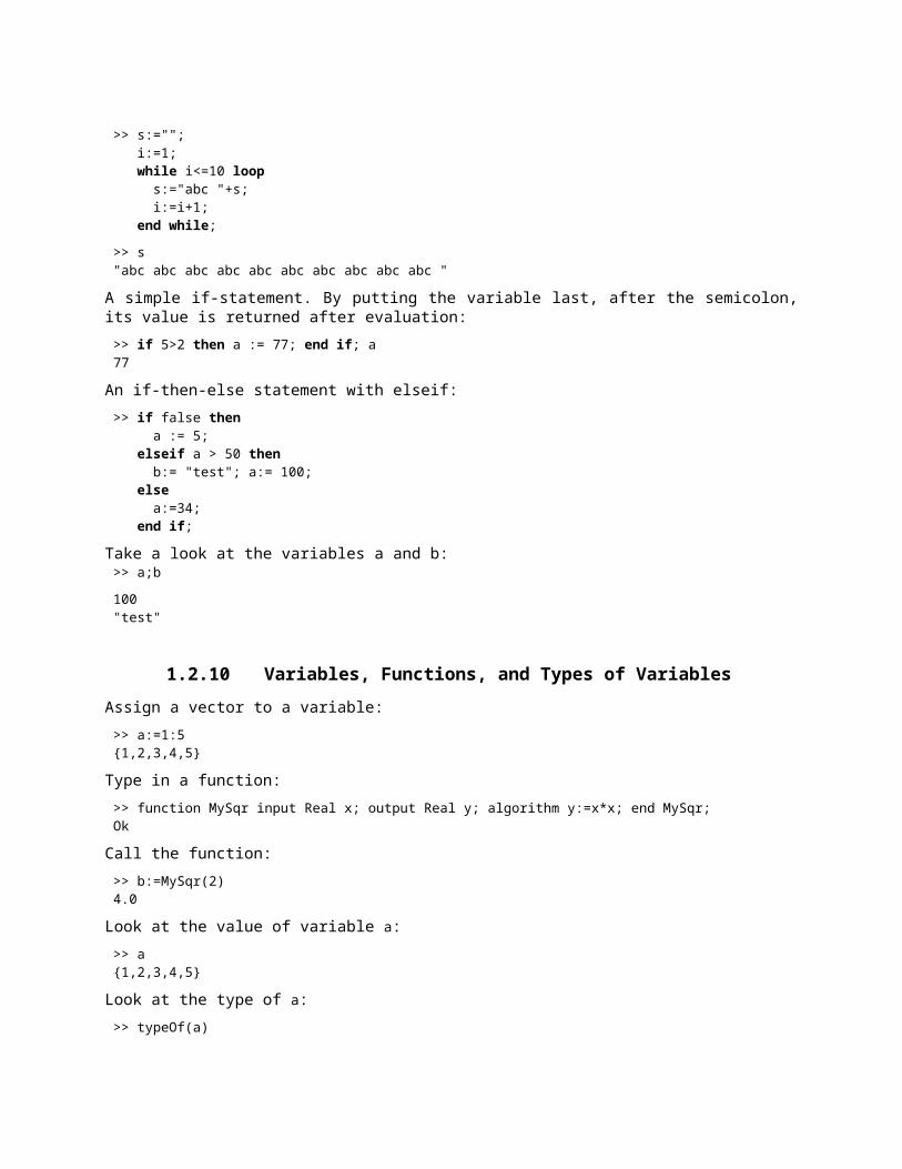
Normal while-loop with concatenation of 10 "abc " strings:>> s:=""; i:=1; while i<=10 loop s:="abc "+s; i:=i+1; end while;

>> s"abc abc abc abc abc abc abc abc abc abc "

A simple if-statement. By putting the variable last, after the semicolon, its value is returned after evaluation:>> if 5>2 then a := 77; end if; a77

An if-then-else statement with elseif:>> if false then

a := 5; elseif a > 50 then b:= "test"; a:= 100; else a:=34; end if;

Take a look at the variables a and b:>> a;b

100"test"

1.2.10 Variables, Functions, and Types of VariablesAssign a vector to a variable:>> a:=1:5{1,2,3,4,5}

Type in a function:>> function MySqr input Real x; output Real y; algorithm y:=x*x; end MySqr;Ok

Call the function:>> b:=MySqr(2)4.0

Look at the value of variable a:>> a{1,2,3,4,5}

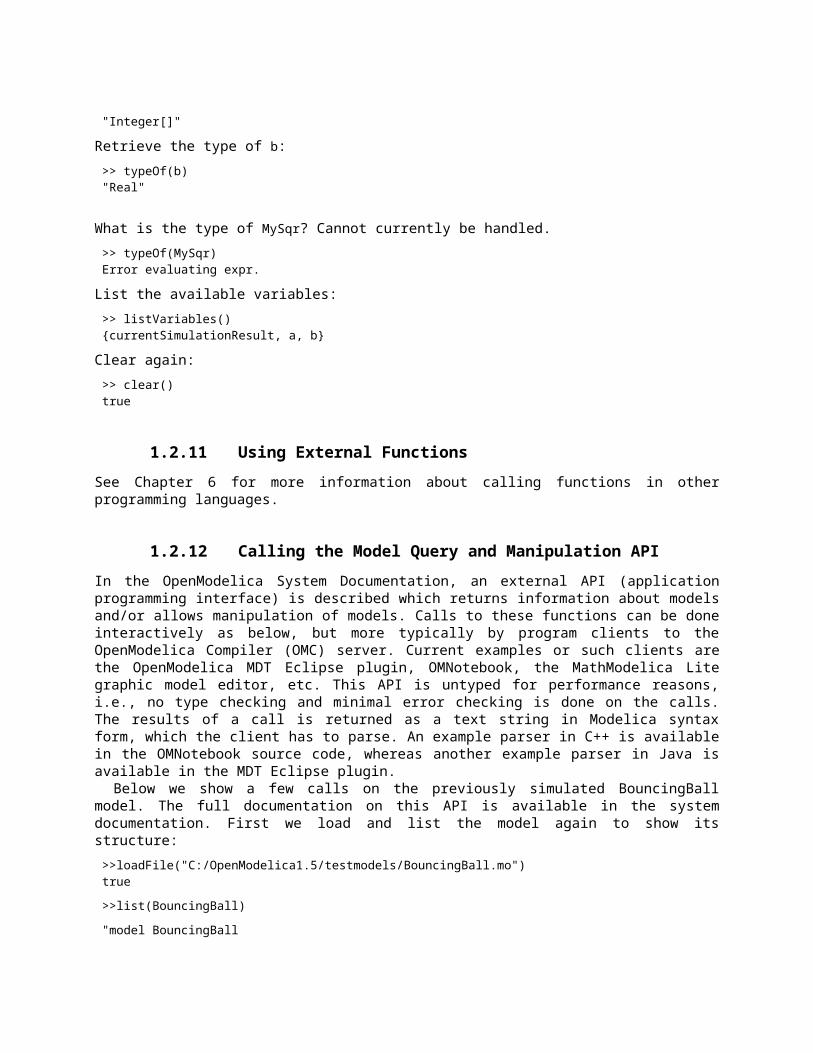
Look at the type of a:>> typeOf(a)"Integer[]"

Retrieve the type of b:>> typeOf(b)"Real"

What is the type of MySqr? Cannot currently be handled.>> typeOf(MySqr)Error evaluating expr.

List the available variables:>> listVariables(){currentSimulationResult, a, b}

Clear again:>> clear()true

1.2.11 Using External FunctionsSee Chapter 6 for more information about calling functions in other programming languages.

1.2.12 Calling the Model Query and Manipulation APIIn the OpenModelica System Documentation, an external API (application programming interface) is described which returns information about models and/or allows manipulation of models. Calls to these functions can be done interactively as below, but more typically by program clients to the OpenModelica Compiler (OMC) server. Current examples or such clients are the OpenModelica MDT Eclipse plugin, OMNotebook, the MathModelica Lite graphic model editor, etc. This API is untyped for performance reasons, i.e., no type checking and minimal error checking is done on the calls. The results of a call is returned as a text string in Modelica syntax form, which the client has to parse. An example parser in C++ is available in the OMNotebook source code, whereas another example parser in Java is available in the MDT Eclipse plugin.

Below we show a few calls on the previously simulated BouncingBall model. The full documentation on this API is available in the system documentation. First we load and list the model again to show its structure:>>loadFile("C:/OpenModelica1.5/testmodels/BouncingBall.mo")true

>>list(BouncingBall)

"model BouncingBall parameter Real e=0.7 "coefficient of restitution"; parameter Real g=9.81 "gravity acceleration"; Real h(start=1) "height of ball"; Real v "velocity of ball"; Boolean flying(start=true) "true, if ball is flying"; Boolean impact; Real v_new;equation impact=h <= 0.0; der(v)=if flying then -g else 0; der(h)=v; when {h <= 0.0 and v <= 0.0,impact} then v_new=if edge(impact) then -e*pre(v) else 0; flying=v_new > 0; reinit(v, v_new); end when;end BouncingBall;"

Different kinds of calls with returned results:>>getClassRestriction(BouncingBall)"model"

>>getClassInformation(BouncingBall){"model","","",{false,false,false},{"writable",1,1,18,17}}

>>isFunction(BouncingBall)false

>>existClass(BouncingBall)true

>>getComponents(BouncingBall){{Real,e,"coefficient of restitution", "public", false, false, false,"parameter", "none", "unspecified"},

{Real,g,"gravity acceleration","public", false, false, false, "parameter", "none", "unspecified"},{Real,h,"height of ball", "public", false, false, false,"unspecified", "none", "unspecified"},{Real,v,"velocity of ball","public", false, false, false, "unspecified", "none", "unspecified"},{Boolean,flying,"true, if ball is flying", "public", false, false,false, "unspecified", "none", "unspecified"},{Boolean,impact,"","public", false, false, false, "unspecified", "none", "unspecified"},{Real,v_new,"", "public", false, false, false, "unspecified", "none","unspecified"}}

>>getConnectionCount(BouncingBall)0

>>getInheritanceCount(BouncingBall)0

>>getComponentModifierValue(BouncingBall,e)0.7

>>getComponentModifierNames(BouncingBall,e){}

>>getClassRestriction(BouncingBall)"model"

>>getVersion() // Version of the currently running OMC"1.5"

1.2.13 Quit OpenModelicaLeave and quit OpenModelica:>> quit()

1.2.14 Dump XML RepresentationThe command dumpXMLDAE dumps an XML representation of a model, according to several optional parameters.dumpXMLDAE(modelname[,asInSimulationCode=<Boolean>] [,filePrefix=<String>] [,storeInTemp=<Boolean>] [,addMathMLCode =<Boolean>])

This command dumps the mathematical representation of a model using an XML representation, with optional parameters. In particular, asInSimulationCode defines where to stop in the translation process (before dumping the model), the other options are relative to the file storage: filePrefix for specifying a different name and storeInTemp to use the temporary directory. The optional parameter addMathMLCode gives the possibility to don't print the MathML code within the xml file, to make it more readable.Usage is trivial, just: addMathMLCode=true/false (default value is false).

1.2.15 Dump Matlab RepresentationThe command export dumps an XML representation of a model, according to several optional parameters.

exportDAEtoMatlab(modelname);

This command dumps the mathematical representation of a model using a Matlab representation. Example:$ cat daequery.mosloadFile("BouncingBall.mo");exportDAEtoMatlab(BouncingBall);readFile("BouncingBall_imatrix.m");

$ omc daequery.mos true"The equation system was dumped to Matlab file:BouncingBall_imatrix.m"

"% Incidence Matrix% ====================================% number of rows: 6IM={[3,-6],[1,{'if', 'true','==' {3},{},}],[2,{'if', 'edge(impact)' {3},{5},}],[4,2],[5,{'if', 'true','==' {4},{},}],[6,-5]};VL = {'foo','v_new','impact','flying','v','h'};

EqStr = {'impact = h <= 0.0;','foo = if impact then 1 else 2;','when {h <= 0.0 AND v <= 0.0,impact} then v_new = if edge(impact) then (-e) * pre(v) else 0.0; end when;','when {h <= 0.0 AND v <= 0.0,impact} then flying = v_new > 0.0; end when;','der(v) = if flying then -g else 0.0;','der(h) = v;'};

OldEqStr={'fclass BouncingBall','parameter Real e = 0.7 "coefficient of restitution";','parameter Real g = 9.81 "gravity acceleration";','Real h(start = 1.0) "height of ball";','Real v "velocity of ball";','Boolean flying(start = true) "true, if ball is flying";','Boolean impact;','Real v_new;','Integer foo;','equation',' impact = h <= 0.0;',' foo = if impact then 1 else 2;',' der(v) = if flying then -g else 0.0;',' der(h) = v;',' when {h <= 0.0 AND v <= 0.0,impact} then',' v_new = if edge(impact) then (-e) * pre(v) else 0.0;',' flying = v_new > 0.0;',' reinit(v,v_new);',' end when;','end BouncingBall;',''};"

1.3 Summary of Commands for the Interactive Session HandlerThe following is the complete list of commands currently available in the interactive session hander.simulate(modelname) Translate a model named modelname and simulate it.simulate(modelname[,startTime=<Real>][,stopTime=<Real>][,numberOfIntervals

=<Integer>]) Translate and simulate a model, with optional start time, stop time, and optional number of simulation intervals or steps for which the simulation results will be computed. Many steps will give higher time resolution, but occupy more space and take longer to compute. The default number of intervals is 500.

plot(vars) Plot the variables given as a vector or a scalar, e.g. plot({x1,x2}) or plot(x1).

plotParametric(var1, var2) Plot var2 relative to var1 from the most recently simulated model, e.g. plotParametric(x,y).

cd() Return the current directory.cd(dir) Change directory to the directory given as string.clear() Clear all loaded definitions.

clearVariables() Clear all defined variables.dumpXMLDAE(modelname, ...) Dumps an XML representation of a model, according to several optional

parameters.exportDAEtoMatlab(name) Dumps an Matlab representation of a model.

instantiateModel(modelname)Performs code instantiation of a model/class and return a string containing the flat class definition.

list() Return a string containing all loaded class definitions.list(modelname) Return a string containing the class definition of the named class.listVariables() Return a vector of the names of the currently defined variables.loadModel(classname) Load model or package of name classname from the path indicated by the

environment variable OPENMODELICALIBRARY.loadFile(str) Load Modelica file (.mo) with name given as string argument str.readFile(str) Load file given as string str and return a string containing the file content.runScript(str) Execute script file with file name given as string argument str.system(str) Execute str as a system(shell) command in the operating system; return

integer success value. Output into stdout from a shell command is put into the console window.

timing(expr) Evaluate expression expr and return the number of seconds (elapsed time) the evaluation took.

typeOf(variable) Return the type of the variable as a string.saveModel(str,modelname) Save the model/class with name modelname in the file given by the string

argument str.help() Print this helptext (returned as a string).quit() Leave and quit the OpenModelica environment

1.4 ReferencesPeter Fritzson, Peter Aronsson, Håkan Lundvall, Kaj Nyström, Adrian Pop, Levon Saldamli, and David Broman. The OpenModelica Modeling, Simulation, and Software Development Environment. In Simulation News Europe, 44/45, December 2005. See also: http://www.openmodelica.org.

Peter Fritzson. Principles of Object-Oriented Modeling and Simulation with Modelica 2.1, 940 pp., ISBN 0-471-471631, Wiley-IEEE Press, 2004.

The Modelica Association. The Modelica Language Specification Version 3.0, Sept 2007. http://www.modelica.org.

Chapter 2

Using the Graphical Model Editor

This chapter just presents a very simple example of using graphical modeling of Modelica models using the SimForge graphical editor that can be used together with OpenModelica. More detailed documentation is available at: http://trac.elet.polimi.it/simforge.

A model is built using the graphical model editor by using drag-and-drop of already developed and freely available model components from the Modelica Standard Library.

2.1 Getting StartedInstall Java, OpenModelica and SimForge according to the Installation Notes.

Important: when launching SimForge for the first time, go to Tools|Settings, and set the paths.

On Windows machines:

OPENMODELICAHOME contains the OpenModelica root directory, e.g., C:\OpenModelica1.5 OPENMODELICALIBRARY points to the directory which contains the Modelica directory of your

favourite Modelica Standard Library package; you can use the one provided with the OpenModelica installation, e.g., C:\OpenModelica1.5\ModelicaLibrary

LD_LIBRARY_PATH is irrelevant

On linux machines:

OPENMODELICAHOME must point to the directory which contains the bin subdirectory where the omc (OpenModelica compiler) executable is located, e.g., /usr/share/openmodelica-1.4/

OPENMODELICALIBRARY points to the directory which contains the Modelica directory of your favourite Modelica Standard Library package, e.g., /usr/share/openmodelica-1.4/modelica-2.2/

LD_LIBRARY_PATH points to the directory containing the libmico library; you can use the one provided by your OpenModelica installation, e.g. /usr/lib/mico-openmodelica-1.4

These will be the default choices for all the new projects which are created. They can be overridden within each project by using project-specific settings.

2.2 Creating a new projectGo to File|New project. Choose a name for the project - this will be the name of the directory containing all project files, so it must be a legal directory name - and select the path where you want this new directory to be created.

SimForge will create the project directory, which contains: the IEC61131 directory, for IEC 61131 controllers code, the Modelica directory, for Modelica code, the Results directory, for permanent storage of simulation results, the Temp directory for temporary files, and the Properties.xml file for the project properties.

Double-click on the Modelica node of the project tree. The three nodes contain the following elements:

Used external packages: all the packages which are used by the project, but which are not part of the project itself, so they are read-only, and are not contained within the project directory. Examples: the Modelica Standard Library, or any other free or commercial third-party library that will be used by the current project.

Modelica classes: a tree view of all the models and packages defined within the project, irrespective of their actual representation as single files or structured entities (i.e., sub-directories). Models within this tree can be edited in both graphics and textual modes.

Modelica files: a view of all the .mo files contained in the project. Can be useful to inspect files, and rearrange the file contents. Text-only editing.

At this point you can create one or more top-level models or packages, which will be saved in the Modelica subdirectory of the project. For instance, right-click on Modelica classes and type TestPackage as the package name, Package as the class type. If you leave 'structured entity' unchecked, the package will be saved as a single .mo file, otherwise it will be saved as a sub-directory containing a package.mo file plus files for all other contained classes.

Now right-click on TestPackage in the project tree, select 'Add class', then type in ModelA and select model as the type of class.

Double-click on the ModelA node to open the text and graphical editors. You can now start editing your model. The three icons on the right of the tool bar can be used to check the model, compile and simulate it, and to show the omc console.

You can now customize the project properties. Click on Tools|Project properties. The General tab provides information about the project's path, as well as some user-defined comments to the project.

The Modelica tab contain the following settings:

The OPENMODELICAHOME, OPENMODELICALIBRARY, and LD_LIBRARY_PATH paths for this project. By default these are set to the tool settings, but it is possible to customize them by clicking on the checkbox and providing a new path, so that each project can use its own version of OMC, Modelica Standard Library, and OMC runtime libraries.

A checkbox to load the Modelica Standard Library. If you want to use the Modelica Standard Library for your project, you have to set this checkbox explicitly when you first create the project, and make sure you then click on the Reload omc button, so that omc loads the standard library, and makes it visible immediately in the project tree. This is not necessary when you later re-open the project, as the required Modelica library will be loaded automatically.

Additional external libraries: you can add them here by giving the paths of the packages. They will show up under the Used external packages node of the project tree, as read-only classes.

Note that it is possible to load multiple projects at the same time in SimForge. They can be selected by the drop-down menu on top of the project tree. Each project talks to a separate instance of OMC, so it is possible to open different projects using different versions of OpenModelica and standard library at the same time within a single instance of the SimForge application. It is also possible to load two different projects that contain two different versions of the same package (thus with the same name). All the class editing windows contain information about the project name, so that there's no chance of being confused.

2D Plotting and 3D Animation

This chapter covers 2D plotting available from OMNotebook, OMShell or programmable plotting from your own Modelica model. The 3D animation is currently available only from OMNotebook (and not on Mac).

2.3 Enhanced Qt-based 2D Plot FunctionalityStarting with OpenModelica 1.4.5, new enhanced plotting functionality is available (Eriksson, 2008). The new plotting is implemented based on a Qt-based (Trolltech, 2007) GUI package. This new plotting functionality has additional features compared to the old Java-based PtPlot plotting. The simulation data is sent directly to the plotting window in OMNotebook (or a popup window if called from OMShell), which handles the presentation (see Figure 3-2). As OMNotebook now has access to all source data it is now be possible to manipulate diagrams, e.g. zoom or change scales.

To allow the use of graphics functions from within Modelica models a new Modelica interface has been developed. This utilizes an external library to communicate with OMNotebook. In addition to this, a number of new functions that can be used for drawing geometric objects like circles, rectangles and lines have been added.

The following is a summary of the capabilities of the new 2D graphics package:

Interaction with OMNotebook. The graphics package has been developed to be fully integrated with OMNotebook and allow modifications of diagrams that have been previously created.

Usage without OMNotebook. If the functionality of the graphics package is used without OMNotebook, a new window should be opened to present the resulting graphics.

Logarithmic scaling. Some applications of OpenModelica produce simulation data with large value ranges, which is hard to make good plots of. One solution to this problem is to scale the diagram logarithmically, and this is allowed by the graphics package.

Zoom. To allow studying of small variations the user is allowed to zoom in and out in a diagram. Support for graphic programming. To allow creation of Modelica models that are able to draw

illustrations, show diagrams and suchlike, it is possible to use the graphics package not only from the external API of OMC, but also from within Modelica models. To accomplish this a new Modelica interface for the graphics package has been created.

Programmable Modelica API. The Modelica API is defined by a number of Modelica functions, located in the package Modelica.Graphics.Plot, which use external libraries to access functionality of the graphics package.

The programmable Modelica API functions include the following:

plot(x). Draws a two-dimensional line diagram of x as a function of time. plotParametric(x,y). Draws a two-dimensional parametric diagram with y as a function of x. plotTable([x1, .., y1; .. ; xn, .., yn]). Draws a two-dimensional parametric diagram with y as a function

of x. drawRect(x1, x2, y1, y2). Draws a rectangle with vertices in (x1, y1) and (x2, y2). drawEllipse(x1, x2, y1, y2). Draws an ellipse with the size of a rectangle with vertices in (x1, y1) and

(x2, y2). drawLine(x1, x2, y1, y2). Draws a line from (x1, y1) to (x2, y2).

Figure 3-2. Plotting architecture with the new 2D graphics package.

2.4 Simple 2D PlotTo create a simple time plot the model HelloWorld defined in DrModelica is simulated. To reduce the amount of simulation data in this example the number of intervals is limited with the argument numberOfIntervals=10. The simulation is started with the command below.simulate(HelloWorld, startTime=0, stopTime=4, numberOfIntervals=10);

When the simulation is finished the file HelloWorld res.plt contains the simulation data. The contents of the file is the following (some formatting has been applied).0 14.440892098500626e-013 0.99999999999955590.4444444444444444 0.64118038842993490.8888888888888888 0.4111122905071631.333333333333333 0.26359713811572491.777777777777778 0.16901331540605872.222222222222222 0.10836802322188132.666666666666667 0.069483451222796233.111111111111112 0.044551426244477873.555555555555556 0.028565500784541384 0.01831563888872685

Diagrams are now created with the new graphics package by using the following command.plot(x);

seems to correspond well with the data.

Figure 3-3. Simple 2D plot of the HelloWorld example.

By re-simulating and saving results at many more points, e.g. using the default 500 intervals, a much smoother plot can be obtained.simulate(HelloWorld, startTime=0, stopTime=4, numberOfIntervals=500);

plot(x);

Figure 3-4. Simple 2D plot of the HelloWorld example with larger number of points.

Additional features of the new plotting are shown in Figure 3-5 and Figure 3-6.

Figure 3-5. Features of the new Qt-based Plotting Package: Show data points, Change line colors, etc.

Figure 3-6. Features of the new Qt-based Plotting Package: Zoom, Fit in view, Grid, etc.

2.4.1 All Plot Functions and their OptionsThe plot functions can be used in a number of ways, depending on the arguments that are included with the call. The following calls are supported.

All of

Command Descriptionplot(x) Creates a diagram with data from the last simulation that

had a variable named x.plot({x,y,..., z}) Like the previous command, but with several variables.plot(model, x) Creates a diagram with data from the previously simulated

model model.plot(model, {x,y,..., z}) Like the previous, but with several variables.plotParametric(x, y) Creates a parametric diagram with data from the last

simulated variables named x and y.plotParametric(model, x, y)

Creates a parametric diagram with data from the previously simulated model model.

plotAll() Creates a diagram with all variables from the last simulated model as functions of time.

plotAll(model) Creates a diagram with all variables from the model model as functions of time.

these commands can have any number of optional arguments to further customize the the resulting diagram. The available options and their allowed values are listed below.

Option Default value Descriptiongrid true Determines whether or not a grid is shown in the

diagram.title "Plot by OpenModelica" This text will be used as the diagram title.interpolation linear Determines if the simulation data should be interpolated

to allow drawing of continuous lines in the diagram. "linear" results in linear interpolation between data points, "constant" keeps the value of the last known data point until a new one is found and "none" results in a diagram where only known data points are plotted.

legend true Determines whether or not the variable legend is shown.points true Determines whether or not the data points should be

indicated by a dot in the diagram.logX false Determines whether or not the horizontal axis is

logarithmically scaled.logY false Determines whether or not the vertical axis is

logarithmically scaled.xRange {0, 0} Determines the horizontal interval that is visible in the

diagram. {0, 0} will select a suitable range.yRange {0, 0} Determines the vertical interval that is visible in the

diagram. {0, 0} will select a suitable range.antiAliasing false Determines whether or not antialiasing should be used

in the diagram to improve the visual quality.vTitle “” This text will be used as the vertical label in the

diagram.hTitle “time” This text will be used as the horizontal label in the

diagram.

2.4.2 ZoomingThe left mouse button can for instance be used for zooming in on interesting parts of the diagram.The same result can be achieved by using the optional parameters xRange and yRange. The plotParametric command would then look like the following.plotParametric(x, y, xRange={0.9, 1.95}, yRange={-1.5, 1.35})

Figure 3-7. Zooming in an Input cell.

Figure 3-8. Magnified input cell.

2.4.3 Plotting all variables of a modelA command, plotAll, has been introduced to plot all the variables of a model. This can be useful if a model contains many interesting variables, as it might be easier to remove variables that are not important than to list all those who are. The commands available for this are plotAll() and plotAll(model). If the optional model parameter is omitted the last simulated model will be used. The command below applies plotAll to the model HelloWorld. The result is shown in Figure 3-9. The simplest way to remove unimportant variables is to use the Remove command in the Legend menu..plotAll(HelloWorld);

Figure 3-9. Result of the plotAll command.

2.4.4 Plotting During SimulationWhen running long simulations, or if plotting without need for commands like plot or plotParametric is desired, the interface for transfer of simulation data during running simulations can be used. This is enabled by running the following command.enableSendData(true)

The same command, but with the parameter false, is used to disable the interface. Enabling of the interface has some drawbacks though. The simulation time will be longer as the transfer of data will require some resources.

If the simulation data would have been plotted anyway, some of this time will be saved later however. To reduce the amount of data that has to be transferred, and thereby reduce the time needed to do so, the interesting variables in the model can be specified with the command setVariableFilter. If for instance the model HelloWorld is to be simulated the following commands can be used.class HelloWorld Real x(start = 1); parameter Real a = 1;equation der(x) = - a * x;end HelloWorld;

enableSendData(true);setVariableFilter({x});simulate(HelloWorld, startTime=0, stopTime=25);

When the simulation data has been transferred the button D will appear to the right of the input field. By pressing this the dialog Simulation data will appear, where new curves can be created.

2.4.5 Programmable Drawing of 2D GraphicsThe graphics package provides functions for drawing of basic geometrical objects in the graphics area. These can be used from Modelica models and are executed when the model is simulated. To avoid name conflicts, the

functions have been put in the package Modelica.pltpkg. The functions of the Modelica programmable plotting interface are described below.

plot(model, "x"). Creates a diagram with data from the variable x in the previously simulated model model.

plot(model, "x, y"). Like the function above, but with more than one variable. plotParametric(model, "x", "y"). Creates a parametric diagram with data from the variables x and y

in the previously simulated model model. plotTable([x1, y1, z1, ...; x2, y2, z2, ...;...]). Draws y and z as functions of x.. clear().Clears the active GraphWidget.

rect(x1, x2, y1, y2). Draws a rectangle with vertices in (x1, y1) and (x2, y2). ellipse(x1, x2, y1, y2). Draws an ellipse with the size of a rectangle with vertices in (x1, y1) and (x2,

y2). line(x1, x2, y1, y2). Draws a line from (x1, y1) to (x2, y2). hold(Boolean on). Determines whether or not the active GraphWidget should be cleared before new

graphics is drawn. wait(ms). Waits for (at least) ms milliseconds.

The following model shows how these functions can be used to draw ellipses, rectangles, and lines.

model testGeom parameter Integer n=10; protected Boolean b[n,n];equation for x in 1:n loop for y in 1:n loop when initial() then if((y == 1) or (y == 10) or (x == 1) or (x == 10)) then b[x,y] = pltpkg.rect(x, y, x+1, y+1, fillColor = "blue", color = "green"); else if(y >= 4 and y <= 5 and x >= 4 and x <= 5) then b[x,y] = pltpkg.line(x, y, x+1, y+1, color = "red"); else b[x,y] = pltpkg.ellipse(x, y, x+1, y+1, fillColor = "yellow", color = "black"); end if; end if; end when; end for; end for;end testGeom;

Figure 3-10. Programmable drawing of rectangles and ellipses.

2.4.6 Plotting of table dataAnother way to visualize data provided by the graphics package is plotting of table data. This is done by using the command pltpkg.plotTable, which expects a matrix of Real values as a parameter. The rows of this matrix represent variable values. The first column is the time variable and the other columns contains values at these points in time. The names of the variables can be specified with the argument variableNames, which is a String list. The following model demonstrates how this command can be used.model table protected Boolean b;algorithm b := pltpkg.pltTable([ 0, 0.95, 0.92, 20, 25; 10, 0.94, 0.92, 23, 28; 20, 0.94, 0.91, 32, 35; 30, 0.93, 0.90, 43, 46] );end table;

The result is shown in Figure 3-11

Figure 3-11. Plotting of table data..

2.5 Java-based PtPlot 2D plottingThe plot functionality in OpenModelica 1.4.4 and earlier was based on PtPlot (Lee, 2006), a Java-based plot package produced within the Ptolemy project. To plot one uses plot commands within input cells which it evaluates. Available plotting commands which calls Java-based plotting are as follows, still available but renamed with a suffix 2:// normal one variable plotting, time on the X axisplot2( variable );// normal multiple variable plotting, time on the X axisplot2( {variable1, variable2, variable3, … variableN} );

// to plot dependent valuesplotParametric2( variableX, variableY );

For example:simulate(HelloWorld, startTime=9, stopTime=4);plot(x);

Figure 3-12. Java-based PtPlot plot window.

2.6 3D AnimationThere are two main approaches to add 3D graphics information to Modelica objects:

Graphical annotations Graphical objects

Both of these approaches were investigated, but the second was finally chosen.

2.6.1 Object Based VisualizationSince one important goal of this work is to come up with a system for visualization that might be used for simulations done with the Modelica MultiBody library (Otter, 2008), it follows that much can be learned from investigating currently available solutions. There are commercial software packages available that can visualize MultiBody simulations.

The MultiBody package is well suited for visualization. Entities in a MultiBody simulation correspond to physical entities in a real world and as such have many of the properties needed to correctly display them within a visualization of the simulation, such as position and rotation. Other properties such as color and shape can easily be added as properties or be decided based on the object type.

Instead of using annotations to encode information about how a certain object is supposed to look when visualized, object based visualization creates additional Modelica objects of a predetermined type that can be known to the client actually doing the visualization. These objects contain variables such as position, rotation and size that can be connected to the simulated variables using ordinary Modelica equations. When asked to visualize a model, the OpenModelica compiler can find variables in the model that are in the visualization package and only send only those datasets over to the client doing the visualization, in this case OMNotebook.

Taking inspiration from the MultiBody library, a small package has been designed that provides a minimal set of classes that can be connected to variables in the simulation. It is created as a Modelica package and can be included in the Modelica Library. The package is called SimpleVisual, and consists of a small hierarchy of classes that in increasing detail can describe properties of a visualized object. It is implemented on top of the Qt graphics package called Coin3D (Coin3D, 2008). More information is available in (Magnusson, 2008). A comprehensive earlier work on integrating and generating 3D graphics from Modelica models is reported in (Engelson, 2000).

This section gives a short introduction to how the SimpleVisual package is used.

2.6.2 BouncingBallThe bouncing ball model is a simple example to the Modelica language. Adding visualization of the bouncing ball using the SimpleVisual package is very straightforward.model BouncingBall parameter Real e=0.7 "coefficient of restitution"; parameter Real g=9.81 "gravity acceleration"; Real h(start=10) "height of ball"; Real v "velocity of ball"; Boolean flying(start=true) "true, if ball is flying"; Boolean impact; Real v_new;equation impact=h <= 0.0; der(v)=if flying then -g else 0; der(h)=v; when {h <= 0.0 and v <= 0.0,impact} then v_new=if edge(impact) then -e*pre(v) else 0; flying=v_new > 0; reinit(v, v_new); end when;end BouncingBall;

To run a simulation of the bouncing ball, create a new InputCell and call the simulate command. The simulate command takes a model, start time, and an end time as arguments.

simulate(BouncingBall, start=0, end=5s);

2.6.2.1 Adding Visualization

The bouncing ball will be simulated with a red sphere. We will let the variable h control the y position of the sphere. Since the ball has a size and the model describes the bouncing movement of a point, we will use that size to translate the visualization slightly upwards. First, we must import the SimpleVisual package and create an object to visualize. That is done by adding a few lines to the beginning of the BouncingBall model, which we rename to BouncingBall3D to emphasize that we have made some changes:model BouncingBall3Dimport SimpleVisual.*SimpleVisual.PositionSize ball "color=red;shape=sphere;";...

The string "color=red;" is used to set the color parameter of the object and the shape parameter controls how we will display this object in the visualization.

The next step is to connect the position of the ball object to the simulation. Since Modelica is an equation based language, we must have the same number of variables as equations in the model. This means that even though the only aspect of the ball that is really interesting is its y-position, each variable in the ball object must be assigned to an equation. Setting a variable to be constant zero is a valid equation. The SimpleVisual library contains a number of generic objects which gives the user an increasing amount of control.SimpleVisual.PositionSimpleVisual.PositionSizeSimpleVisual.PositionRotationSimpleVisual.PositionRotationSizeSimpleVisual.PositionRotationSizeO_set

Since we are really only interested in the position of the ball, we could use SimpleVisual.Position, but to make it a little bit more interesting we use SimpleVisual.PositionSize and make the ball a little bigger.obj.size[1]=5; obj.size[2]=5; obj.size[3]=5;obj.frame_a[1]=0; obj.frame_a[2]=h+obj.size[2]/2; obj.frame_a[3]=0;

A SimpleVisual.PositionSize object has two properties; size and frame_a. All are three dimensional real numbers, or Real[3] in Modelica.

size controls the size of the visual representation of the object. frame_a contains the position of the object.

2.6.2.2 Running the Simulation and Starting Visualization

To be able to simulate the model with the added visualization, OpenModelica must load the SimpleVisual package.loadLibrary(Modelica.SimpleVisual)

Now, call simulate once more. This time the simulation will generate values for the added SimpleVisual object that can be read by the visualization in OMNotebook.simulate(BouncingBall3D, start=0, end=5s);

To display the visualization, create an input cell and call the visualize in the input part of the cell.visualize(BouncingBall3D);

Figure 3-13. 3D animation of the bouncing ball model.

2.6.3 Pendulum 3D ExampleThis example explores a slightly more complex scenario where the visualization uses all the properties of a SimpleVisual object. The model used is a simple ideal 2D pendulum, not modeling properties like friction, air resistance etc.class MyPendulum3D "Planar Pendulum"constant Real PI=3.141592653589793;parameter Real m=1, g=9.81, L=5;Real F;Real x(start=5),y(start=0);Real vx,vy;equation m*der(vx)=-(x/L)*F; m*der(vy)=-(y/L)*F-m*g; der(x)=vx; der(y)=vy; x^2+y^2=L^2;end MyPendulum3D;

Start by identifying the variables in the model that will be needed to create a visual representation of the simulation.

Real x and Real y hold the current position of the pendulum.

Real L is a parameter which holds the length of the pendulum.

2.6.3.1 Adding the Visualization

As before, to be able to use the SimpleVisual package we must import it.class MyPendulum3D "Planar Pendulum"import Modelica.SimpleVisual;...

Adding a sphere to represent the weight of the pendulum is done in the same way the BouncingBall was visualized. The variables x and y hold the position....Real vx,vy;SimpleVisual.PositionSize ball "color=red;shape=ball;";equation ball.size[1]=1.5; ball.size[2]=1.5; ball.size[3]=1.5; ball.frame_a[1]=x; ball.frame_a[2]=y; ball.frame_a[3]=0; m*der(vx)=-(x/L)*F;...

The next step is to create a visualization of the "thread" that holds the pendulum. It will be represented by a small elongated cube connected to the ball in one end and in the fixed center of the pendulum movement. We will want the object to rotate with the pendulum motion so create a SimpleVisual. PositionRotationSize object.SimpleVisual.PositionRotationSize thread "shape=cube;"

To specify the rotation of an object, the visualization package uses two points. One is the position of the object, frame_a, that has been demonstrated earlier. The other position, frame_b, is interpreted as the end point of a vector from frame_a. This vector is used as the new up direction for the object. In this example, defining frame_b is simple. The cube that represents the thread will always be pointing to (0, 0, 0). We already know the length of the thread from the parameter L.thread.size[1]=0.05; thread.size[2]=L; thread.size[3]=0.05;thread.frame_a[1]=x; thread.frame_a[2]=y; thread.frame_a[3]=0;thread.frame_b[1]=0; thread.frame_b[2]=0; thread.frame_b[3]=0;

Running this simulation and starting the visualization, we notice that everything is not quite right. The thread is centered around the pendulum. We could calculate a new position by translating the x and y coordinates along the rotation vector, but there is a better way. Change the object type to SimpleVisual. PositionRotationSizeOffset. The offset parameter is a translation within the local coordinate system of the object. To shift the center of the object to be at the bottom of the thread we add an offset of L/2 to the y component of offset.thread.size[1]=0.05; thread.size[2]=L; thread.size[3]=0.05;thread.frame_a[1]=x; thread.frame_a[2]=y; thread.frame_a[3]=0;thread.frame_b[1]=0; thread.frame_b[2]=0; thread.frame_b[3]=0;thread.offset[1]=0; thread.offset[2]=L/2; thread.offset[3]=0;

In the final model, a simple static fixture has also been added.class MyPendulum3D "Planar Pendulum" import Modelica.SimpleVisual; constant Real PI=3.141592653589793; parameter Real m=1, g=9.81, L=5; Real F; Real x(start=5),y(start=0); Real vx,vy;

SimpleVisual.PositionSize ball "color=red;shape=ball;"; SimpleVisual.PositionSize fixture "shape=cube;"; SimpleVisual.PositionRotationSizeOffset thread "shape=cube;";equation fixture.size[1]=0.5; fixture.size[2]=0.1; fixture.size[3]=0.5; fixture.frame_a[1]=0; fixture.frame_a[2]=0; fixture.frame_a[3]=0; ball.size[1]=1.5; ball.size[2]=1.5; ball.size[3]=1.5; ball.frame_a[1]=x; ball.frame_a[2]=y; ball.frame_a[3]=0; thread.size[1]=0.05; thread.size[2]=L; thread.size[3]=0.05; thread.frame_a[1]=x; thread.frame_a[2]=y; thread.frame_a[3]=0; thread.frame_b[1]=0; thread.frame_b[2]=0; thread.frame_b[3]=0; thread.offset[1]=0; thread.offset[2]=L/2; thread.offset[3]=0; m*der(vx)=-(x/L)*F; m*der(vy)=-(y/L)*F-m*g; der(x)=vx; der(y)=vy; x^2+y^2=L^2;end MyPendulum3D;

We simulate and visualize as previously:

Figure 3-14. Visualization with animation of 3D pendulum.

2.7 ReferencesTrolltech. Qt. http://www.trolltech.com/, accessed July 2007.

Coin3D. www.coin3d.org, accessed August 2008.

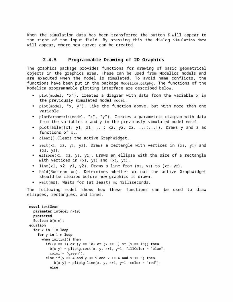
Henrik Eriksson. Advanced OpenModelica Plotting Package for Modelica. Master Thesis, LIU-IDA/LITH-EX-A-08/036-SE, Linköping University Electronic Press, www.ep.liu.se, June 22, 2008.

Henrik Magnusson. Integrated Generic 3D visualization of Modelica Models. Master Thesis, LIU-IDA/LITH-EX-A-08/035-SE, Linköping University Electronic Press, www.ep.liu.se, June 27, 2008.

Martin Otter. The Modelica MultiBody Library. http://www.modelica.org/libraries/Modelica, Modelica.Mechanics.MultiBody, accessed August 2008.

Vadim Engelson. Tools for Design, Interactive Simulation, and Visualization of Object-Oriented Models in Scientific Computing. Ph.D. Thesis. Linköping Studies in Science and Technology, Dissertation No. 627, http://www.ida.liu.se/~vaden/thesis/, 2000.

Edward Lee et al. The PtPlot package The Ptolemy Project. http://ptolemy.berkeley.edu/body.htm, accessed July 2007.

Chapter 3

OMNotebook with DrModelica

This chapter covers the OpenModelica electronic notebook subsystem, called OMNotebook, together with the DrModelica tutoring system for teaching Modelica, which is using such notebooks.

3.1 Interactive Notebooks with Literate ProgrammingInteractive Electronic Notebooks are active documents that may contain technical computations and text, as well as graphics. Hence, these documents are suitable to be used for teaching and experimentation, simulation scripting, model documentation and storage, etc.

3.1.1 Mathematica NotebooksLiterate Programming (Knuth 1984) is a form of programming where programs are integrated with documentation in the same document. Mathematica notebooks (Wolfram 1997) is one of the first WYSIWYG (What-You-See-Is-What-You-Get) systems that support Literate Programming. Such notebooks are used, e.g., in the MathModelica modeling and simulation environment, e.g. see Figure 4-15 below and Chapter 19 in (Fritzson 2004)

3.1.2 OMNotebookThe OMNotebook software (Axelsson 2005, Fernström 2006) is a new open source free software that gives an interactive WYSIWYG (What-You-See-Is-What-You-Get) realization of Literate Programming, a form of programming where programs are integrated with documentation in the same document.

The OMNotebook facility is actually an interactive WYSIWYG (What-You-See-Is-What-You-Get) realization of Literate Programming, a form of programming where programs are integrated with documentation in the same document. OMNotebook is a simple open-source software tool for an electronic notebook supporting Modelica.

A more advanced electronic notebook tool, also supporting mathematical typesetting and many other facilities, is provided by Mathematica notebooks in the MathModelica environment, see Figure 4-15.

Figure 4-15. Examples of Mathematica notebooks in the MathModelica modeling and simulation environment.

Traditional documents, e.g. books and reports, essentially always have a hierarchical structure. They are divided into sections, subsections, paragraphs, etc. Both the document itself and its sections usually have headings as labels for easier navigation. This kind of structure is also reflected in electronic notebooks. Every notebook corresponds to one document (one file) and contains a tree structure of cells. A cell can have different kinds of contents, and can even contain other cells. The notebook hierarchy of cells thus reflects the hierarchy of sections and subsections in a traditional document such as a book..

3.2 The DrModelica Tutoring System – an Application of OMNotebookUnderstanding programs is hard, especially code written by someone else. For educational purposes it is essential to be able to show the source code and to give an explanation of it at the same time.

Moreover, it is important to show the result of the source code’s execution. In modeling and simulation it is also important to have the source code, the documentation about the source code, the execution results of the simulation model, and the documentation of the simulation results in the same document. The reason is that the problem solving process in computational simulation is an iterative process that often requires a modification of the original mathematical model and its software implementation after the interpretation and validation of the computed results corresponding to an initial model.

Most of the environments associated with equation-based modeling languages focus more on providing efficient numerical algorithms rather than giving attention to the aspects that should facilitate the learning and teaching of the language. There is a need for an environment facilitating the learning and understanding of Modelica. These are the reasons for developing the DrModelica teaching material for Modelica and for teaching modeling and simulation.

An earlier version of DrModelica was developed using the MathModelica environment. The rest of this chapter is concerned with the OMNotebook version of DrModelica and on the OMNotebook tool itself.

DrModelica has a hierarchical structure represented as notebooks. The front-page notebook is similar to a table of contents that holds all other notebooks together by providing links to them. This particular notebook is the first page the user will see (Figure 4-16).

Figure 4-16. The front-page notebook of the OMNotebook version of the DrModelica tutoring system.

In each chapter of DrModelica the user is presented a short summary of the corresponding chapter of the book “Principles of Object-Oriented Modeling and Simulation with Modelica 2.1” by Peter Fritzson. The summary introduces some keywords, being hyperlinks that will lead the user to other notebooks describing the keywords in detail.

Figure 4-17. The HelloWorld class simulated and plotted using the OMNotebook version of DrModelica.

Now, let us consider that the link “HelloWorld” in DrModelica Section is clicked by the user. The new HelloWorld notebook (see Figure 4-17), to which the user is being linked, is not only a textual description but

also contains one or more examples explaining the specific keyword. In this class, HelloWorld, a differential equation is specified.

No information in a notebook is fixed, which implies that the user can add, change, or remove anything in a notebook. Alternatively, the user can create an entirely new notebook in order to write his/her own programs or copy examples from other notebooks. This new notebook can be linked from existing notebooks.

Figure 4-18. DrModelica Chapter on Algorithms and Functions in the main page of the OMNotebook version of DrModelica.

When a class has been successfully evaluated the user can simulate and plot the result, as previously depicted in Figure 4-17 for the simple HelloWorld example model..

After reading a chapter in DrModelica the user can immediately practice the newly acquired information by doing the exercises that concern the specific chapter. Exercises have been written in order to elucidate language constructs step by step based on the pedagogical assumption that a student learns better “using the strategy of learning by doing”. The exercises consist of either theoretical questions or practical programming assignments. All exercises provide answers in order to give the user immediate feedback.

Figure 4-18 shows part of Chapter 9 of the DrModelica teaching material. Here the user can read about language constructs, like algorithm sections, when-statements, and reinit equations, and then practice these constructs by solving the exercises corresponding to the recently studied section.

Figure 4-19. Exercise 1 in Chapter 9 of DrModelica.

Exercise 1 from Chapter 9 is shown in . In this exercise the user has the opportunity to practice different language constructs and then compare the solution to the answer for the exercise. Notice that the answer is not visible until the Answer section is expanded. The answer is shown in .

Figure 4-20. The answer section to Exercise 1 in Chapter 9 of DrModelica.

3.3 OpenModelica Notebook CommandsOMNotebook currently supports the commands and concepts that are summarized in this section.

3.3.1 CellsEverything inside an OMNotebook document is made out of cells. A cell basically contains a chunk of data. That data can be text, images, or other cells. OMNotebook has four types of cells: headercell, textcell, inputcell, and groupcell. Cells are ordered in a tree structure, where one cell can be a parent to one or more additional cells. A tree view is available close to the right border in the notebook window to display the relation between the cells.

Textcell – This cell type are used to display ordinary text and images. Each textcell has a style that specifies how text is displayed. The cell´s style can be changed in the menu Format->Styles, example of different styles are: Text, Title, and Subtitle. The Textcell type also has support for following links to other notebook documents.

Inputcell – This cell type has support for syntax highlighting and evaluation. It is intended to be used for writing program code, e.g. Modelica code. Evaluation is done by pressing the key combination Shift+Return or Shift+Enter. All the text in the cell is sent to OMC (OpenModelica Compiler/interpreter), where the text is evaluated and the result is displayed below the inputcell. By double-clicking on the cell marker in the tree view, the inputcell can be collapsed causing the result to be hidden.

Groupcell – This cell type is used to group together other cell. A groupcell can be opened or closed. When a groupcell is opened all the cells inside the groupcell are visible, but when the groupcell is closed only the first cell inside the groupcell is visible. The state of the groupcell is changed by the user double-clicking on the cell marker in the tree view. When the groupcell is closed the marker is changed and the marker has an arrow at the bottom.

3.3.2 CursorsAn OMNotebook document contains cells which in turn contain text. Thus, two kinds of cursors are needed for positioning, text cursor and cell cursor:

Textcursor – A cursor between characters in a cell, appearing as a small vertical line. Position the cursor by clicking on the text or using the arrow buttons.

Cellcursor – This cursor shows which cell currently has the input focus. It consists of two parts. The main cellcursor is basically just a thin black horizontal line below the cell with input focus. The cellcursor is positioned by clicking on a cell, clicking between cells, or using the menu item Cell->Next Cell or Cell->Previous Cell. The cursor can also be moved with the key combination Ctrl+Up or Ctrl+Down. The dynamic cellcursor is a short blinking horisontal line. To make this visible, you must click once more on the main cellcursor (the long horizontal line). NOTE: In order to paste cells at the cellcursor, the dynamic cellcursor must be made active by clicking on the main cellcursor (the horisontal line).

3.4 Selection of Text or CellsTo perform operations on text or cells we often need to select a range of characters or cells.

Select characters – There are several ways of selecting characters, e.g. double-clicking on a word, clicking and dragging the mouse, or click followed by a shift-click at an adjacent positioin selects the text between the previous click and the position of the most recent shift-click.

Select cells – Cells can be selected by clicking on them. Holding done Ctrl and clicking on the cell markers in the tree view allows several cells to be selected, one at a time. Several cells can be

selected at once in the tree view by holding down the Shift key. Holding down Shift selects all cells between last selected cell and the cell clicked on. This only works if both cells belong to the same groupcell.

3.4.1 File MenuThe following file related operations are available in the file menu:

Create a new notebook – A new notebook can be created using the menu File->New or the key combination Ctrl+N. A new document window will then open, with a new document inside.

Open a notebook – To open a notebook use File->Open in the menu or the key combination Ctrl+O. Only files of the type .onb or .nb can be opened. If a file does not follow the OMNotebook format or the FullForm Mathematica Notebook format, a message box is displayed telling the user what is wrong. Mathematica Notebooks must be converted to fullform before they can be opened in OMNotebook.

Save a notebook – To save a notebook use the menu item File->Save or File->Save As. If the notebook has not been saved before the save as dialog is shown and a filename can be selected. OMNotebook can only save in xml format and the saved file is not compatible with Mathematica. Key combination for save is Ctrl+S and for save as Ctrl+Shift+S. The saved file by default obtains the file extension .onb.

Print – Printing a document to a printer is done by pressing the key combination Ctrl+P or using the menu item File->Print. A normal print dialog is displayed where the usually properties can be changed.

Import old document – Old documents, saved with the old version of OMNotebook where a different file format was used, can be opened using the menu item File->Import->Old OMNotebook file. Old documents have the extension .xml.

Export text – The text inside a document can be exported to a text document. The text is exported to this document without almost any structure saved. The only structure that is saved is the cell structure. Each paragraph in the text document will contain text from one cell. To use the export function, use menu item File->Export->Pure Text.

Close a notebook window – A notebook window can be closed using the menu item File->Close or the key combination Ctrl+F4. Any unsaved changes in the document are lost when the notebook window is closed.

Quitting OMNotebook – To quit OMNotebook, use menu item File->Quit or the key combination Crtl+Q. This closes all notebook windows; users will have the option of closing OMC also. OMC will not automatically shutdown because other programs may still use it. Evaluating the command quit() has the same result as exiting OMNotebook.

3.4.2 Edit Menu Editing cell text – Cells have a set of of basic editing functions. The key combination for these are:

Undo (Ctrl+Z), Redo (Ctrl+Y), Cut (Ctrl+X), Copy (Ctrl+C) and Paste (Ctrl+V). These functions can also be accessed from the edit menu; Undo (Edit->Undo), Redo (Edit->Redo), Cut (Edit->Cut), Copy (Edit->Copy) and Paste (Edit->Paste). Selection of text is done in the usual way by double-clicking, triple-clicking (select a paragraph), dragging the mouse, or using (Ctrl+A) to select all text within the cell.

Cut cell – Cells can be cut from a document with the menu item Edit->Cut or the key combination Ctrl+X. The cut function will always cut cells if cells have been selected in the tree view, otherwise the cut function cuts text.

Copy cell – Cells can be copied from a document with the menu item Edit->Copy or the key combination Ctrl+C. The copy function will always copy cells if cells have been selected in the tree view, otherwise the copy function copy text.

Paste cell – To paste copied or cut cells the cell cursor must be selected in the location where the cells should be pasted. This is done by clicking on the cell cursor. Pasteing cells is done from the menu Edit->Paste or the key combination Ctrl+V. If the cell cursor is selected the paste function will always paste cells. OMNotebook share the same application-wide clipboard. Therefore cells that have been copied from one document can be pasted into another document. Only pointers to the copied or cut cells are added to the clipboard, thus the cell that should be pasted must still exist. Consequently a cell can not be pasted from a document that has been closed.

Find – Find text string in the current notebook, with the options match full word, match cell, search within closed cells. Short command Ctrl+F.

Replace – Find and replace text string in the current notebook, with the options match full word, match cell, search+replace within closed cells. Short command Ctrl+H.

View expression – Text in a cell is stored internally as a subset of HTML code and the menu item Edit->View Expression let the user switch between viewing the text or the internal HTML representation. Changes made to the HTML code will affect how the text is displayed.

3.4.3 Cell Menu Add textcell – A new textcell is added with the menu item Cell->Add Cell (previous cell style) or

the key combination Alt+Enter. The new textcell gets the same style as the previous selected cell had.

Add inputcell – A new inputcell is added with the menu item Cell->Add Inputcell or the key combination Ctrl+Shift+I.

Add groupcell – A new groupcell is inserted with the menu item Cell->Groupcell or the key combination Ctrl+Shift+G. The selected cell will then become the first cell inside the groupcell.

Ungroup groupcell – A groupcell can be ungrouped by selecting it in the tree view and using the menu item Cell->Ungroup Groupcell or by using the key combination Ctrl+Shift+U. Only one groupcell at a time can be ungrouped.

Split cell – Spliting a cell is done with the menu item Cell->Split cell or the key combination Ctrl+Shift+P. The cell is splited at the position of the text cursor.

Delete cell – The menu item Cell->Delete Cell will delete all cells that have been selected in the tree view. If no cell is selected this action will delete the cell that have been selected by the cellcursor. This action can also be called with the key combination Ctrl+Shift+D or the key Del (only works when cells have been selected in the tree view).

Cellcursor – This cell type is a special type that shows which cell that currently has the focus. The cell is basically just a thin black line. The cellcursor is moved by clicking on a cell or using the menu item Cell->Next Cell or Cell->Previous Cell. The cursor can also be moved with the key combination Ctrl+Up or Ctrl+Down.

3.4.4 Format Menu Textcell – This cell type is used to display ordinary text and images. Each textcell has a style that

specifies how text is displayed. The cells style can be changed in the menu Format->Styles, examples of different styles are: Text, Title, and Subtitle. The Textcell type also have support for following links to other notebook documents.

Text manipulation – There are a number of different text manipulations that can be done to change the appearance of the text. These manipulations include operations like: changing font, changing color and make text bold, but also operations like: changing the alignment of the text and the margin inside the cell. All text manipulations inside a cell can be done on single letters, words or the entire text. Text settings are found in the Format menu. The following text manipulations are available in OMNotebook:

> Font family > Font face (Plain, Bold, Italic, Underline) > Font size > Font stretch > Font color > Text horizontal alignment > Text vertical alignment > Border thickness > Margin (outside the border) > Padding (inside the border)

3.4.5 Insert Menu Insert image – Images are added to a document with the menu item Insert->Image or the key

combination Ctrl+Shift+M. After an image has been selected a dialog appears, where the size of the image can be chosen. The images actual size is the default value of the image. OMNotebook stretches the image accordantly to the selected size. All images are saved in the same file as the rest of the document.

Insert link – A document can contain links to other OMNotebook file or Mathematica notebook and to add a new link a piece of text must first be selected. The selected text make up the part of the link that the user can click on. Inserting a link is done from the menu Insert->Link or with the key combination Ctrl+Shift+L. A dialog window, much like the one used to open documents, allows the user to choose the file that the link refers to. All links are saved in the document with a relative file path so documents that belong together easily can be moved from one place to another without the links failing.

3.4.6 Window Menu Change window – Each opened document has its own document window. To switch between those

use the Window menu. The window menu lists all titles of the open documents, in the same order as they were opened. To switch to another document, simple click on the title of that document.

3.4.7 Help Menu About OMNotebook – Accessing the about message box for OMNotebook is done from the menu

Help->About OMNotebook. About Qt – To access the message box for Qt, use the menu Help->About Qt. Help Text – Opening the help text (document OMNotebookHelp.onb) for OMNotebook can be

done in the same way as any OMNotebook document is opened or with the menu Help->Help Text. The menu item can also be triggered with the key F1.

3.4.8 Additional Features Links – By clicking on a link, OMNotebook will open the document that is referred to in the link. Update link – All links are stored with relative file path. Therefore OMNotebook has functions that

automatically updating links if a document is resaved in another folder. Every time a document is saved, OMNotebook checks if the document is saved in the same folder as last time. If the folder has changed, the links are updated.

Evaluate several cells – Several inputcells can be evaluated at the same time by selecting them in the treeview and then pressing the key combination Shift+Enter or Shift+Return. The cells are evaluated in the same order as they have been selected. If a groupcell is selected all inputcells in that groupcell are evaluated, in the order they are located in the groupcell.

Command completion – Inputcells have command completion support, which checks if the user is typing a command (or any keyword defined in the file commands.xml) and finish the command. If the user types the first two or three letters in a command, the command completion function fills in the rest. To use command completion, press the key combination Ctrl+Space or Shift+Tab. The first command that matches the letters written will then appear. Holding down Shift and pressing Tab (alternative holding down Ctrl and pressing Space) again will display the second command that matches. Repeated request to use command completion will loop through all commands that match the letters written. When a command is displayed by the command completion functionality any field inside the command that should be edited by the user is automatically selected. Some commands can have several of these fields and by pressing the key combination Ctrl+Tab, the next field will be selected inside the command. > Active Command completion: Ctrl+Space / Shift+Tab > Next command: Ctrl+Space / Shift+Tab > Next field in command: Ctrl+Tab’

Generated plot – When plotting a simulation result, OMC uses the program Ptplot to create a plot. From Ptplot OMNotebook gets an image of the plot and automatically adds that image to the output part of an inputcell. Like all other images in a document, the plot is saved in the document file when the document is saved.

Stylesheet –OMNotebook follows the style settings defined in stylesheet.xml and the correct style is applied to a cell when the cell is created.

Automatic Chapter Numbering – OMNotebook automatically numbers different chapter, subchapter, section and other styles. The user can specify which styles should have chapter numbers and which level the style should have. This is done in the stylesheet.xml file. Every style can have a <chapterLevel> tag that specifies the chapter level. Level 0 or no tag at all, means that the style should not have any chapter numbering.

Scrollarea – Scrolling through a document can be done by using the mouse wheel. A document can also be scrolled by moving the cell cursor up or down.

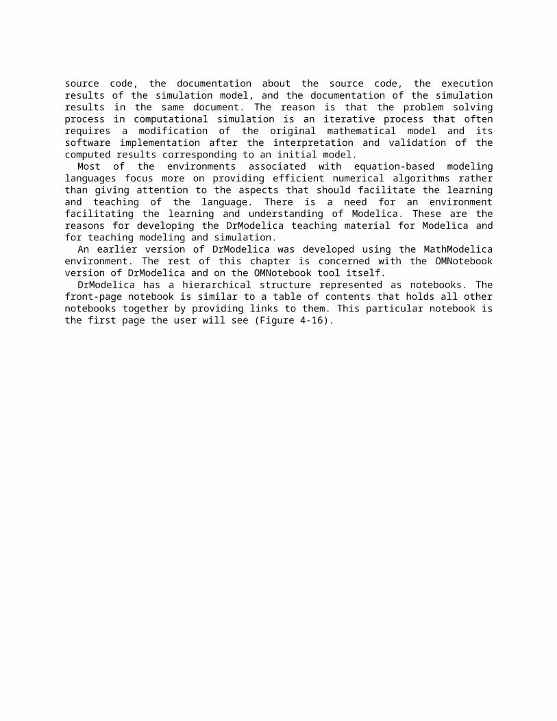
Syntax highlighter – The syntax highlighter runs in a separated thread which speeds up the loading of large document that contains many Modelica code cells. The syntax highlighter only highlights when letters are added, not when they are removed. The color settings for the different types of keywords are stored in the file modelicacolors.xml. Besides defining the text color and background color of keywords, whether or not the keywords should be bold or/and italic can be defined.

Change indicator – A star (*) will appear behind the filename in the title of notebook window if the document has been changed and needs saving. When the user closes a document that has some unsaved change, OMNotebook asks the user if he/she wants to save the document before closing. If the document never has been saved before, the save-as dialog appears so that a filename can be choosen for the new document.

Update menus – All menus are constantly updated so that only menu items that are linked to actions that can be performed on the currently selected cell is enabled. All other menu items will be disabled. When a textcell is selected the Format menu is updated so that it indicates the text settings for the text, in the current cursor position.

3.5 ReferencesEric Allen, Robert Cartwright, Brian Stoler. DrJava: A lightweight pedagogic environment for Java. In Proceedings of the 33rd ACM Technical Symposium on Computer Science Education (SIGCSE 2002) (Northern Kentucky – The Southern Side of Cincinnati, USA, February 27 – March 3, 2002).

Ingemar Axelsson. OpenModelica Notebook for Interactive Structured Modelica Documents. Final thesis, LITH-IDA-EX–05/080–SE, Linköping University, Linköping, Sweden, October 21, 2005.

Anders Fernström, Ingemar Axelsson, Peter Fritzson, Anders Sandholm, Adrian Pop. OMNotebook – Interactive WYSIWYG Book Software for Teaching Programming. In Proc. of the Workshop on Developing Computer Science Education – How Can It Be Done?. Linköping University, Dept. Computer & Inf. Science, Linköping, Sweden, March 10, 2006.

Anders Fernström. Extending OMNotebook – An Interactive Notebook for Structured Modelica Documents. Final thesis, LITH-IDA-EX--06/057—SE, Dept. Computer and Information Science, Linköping University, Sweden, September 4, 2006.

Peter Fritzson. Principles of Object Oriented Modeling and Simulation with Modelica 2.1, 940 pages, ISBN 0-471-471631, Wiley-IEEE Press. Feb. 2004.

Knuth, Donald E. Literate Programming. The Computer Journal, NO27(2), pp. 97–111, May 1984.

Eva-Lena Lengquist-Sandelin, Susanna Monemar, Peter Fritzson, and Peter Bunus. DrModelica – A Web-Based Teaching Environment for Modelica. In Proceedings of the 44th Scandinavian Conference on Simulation and Modeling (SIMS’2003), available at www.scan-sims.org. Västerås, Sweden. September 18-19, 2003.

The Modelica Association. The Modelica Language Specification Version 3.0, Sept 2007. http://www.modelica.org.

Stephen Wolfram. The Mathematica Book. Wolfram Media Inc, 1997.

Chapter 4

MDT – The OpenModelica Development Tooling Eclipse Plugin

4.1 IntroductionThe Modelica Development Tooling (MDT) Eclipse Plug-In as part of OMDev – The OpenModelica Development Environment integrates the OpenModelica compiler with Eclipse. MDT, together with the OpenModelica compiler, provides an environment for working with Modelica development projects.

The following features are available:

Browsing support for Modelica projects, packages, and classes Wizards for creating Modelica projects, packages, and classes Syntax color highlighting Syntax checking Browsing of the Modelica Standard Library or other libraries Code completion for class names and function argument lists. Goto definition for classes, types, and functions. Displaying type information when hovering the mouse over an identifier.

4.2 InstallationThe installation of MDT is accomplished by following the below installation instructions. These instructions assume that you have successfully downloaded and installed Eclipse (http://www.eclipse.org).

1. Start Eclipse2. Select Help->Software Updates->Find and Install... from the menu3. Select ‘Search for new features to install’ and click ‘Next’4. Select ‘New Remote Site...’5. Enter ‘MDT’ as name and ‘http://www.ida.liu.se/labs/pelab/modelica/OpenModelica/MDT’ as

URL and click ‘OK’6. Make sure ‘MDT’ is selected and click ‘Finish’7. In the updates dialog select the ‘MDT’ feature and click ‘Next’8. Read through the license agreement, select ‘I accept...’ and click ‘Next’9. Click ‘Finish’ to install MDT

4.3 Getting Started

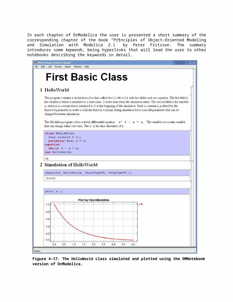
4.3.1 Configuring the OpenModelica CompilerMDT needs to be able to locate the binary of the compiler. It uses the environment variable OPENMODELICAHOME to do so.

If you have problems using MDT, make sure that OPENMODELICAHOME is pointing to the folder where the Open Modelica Compiler is installed. In other words, OPENMODELICAHOME must point to the folder that contains the Open Modelica Compiler (OMC) binary. On the Windows platform it’s called omc.exe and on Unix platforms it’s called omc.

4.3.2 Using the Modelica PerspectiveThe most convenient way to work with Modelica projects is to use to the Modelica perspective. To switch to the Modelica perspective, choose the Window menu item, pick Open Perspective followed by Other... Select the Modelica option from the dialog presented and click OK..

4.3.3 Selecting a Workspace FolderEclipse stores your projects in a folder called a workspace. You need to choose a workspace folder for this session, see Figure 5-21

Figure 5-21. Eclipse Setup – Switching Workspace.

4.3.4 Creating one or more Modelica ProjectsTo start a new project, use the New Modelica Project Wizard. It is accessible through File->New-> Modelica Project or by right-clicking in the Modelica Projects view and selecting New->Modelica Project.

Figure 5-22. Eclipse Setup – creating a Modelica project in the workspace.

You need to disable automatic build for the project(s) (Figure 5-23).

Figure 5-23. Eclipse Setup – disable automatic build for the projects.

Build Automaticallyshould be DISABLEDfor all projects

Repeat the procedure for all the projects you need, e.g. for the exercises described in the MetaModelica users guide: 01_experiment, 02a_exp1, 02b_exp2, 03_assignment, 04a_assigntwotype, etc.

NOTE: Leave open only the projects you are working on! Close all the others!

4.3.5 Building and Running a ProjectAfter having created a project, you eventually need to build the project (Figure 5-24).

Figure 5-24. Eclipse MDT – Building a project.

There are several options: building, building from scratch (clean), running, see Figure 5-25.

Figure 5-25. Eclipse – building and running a project.

leave empty – builds the projectclean – cleans the projectrun – runs the programdebug – builds in debug mode

The problems are inthe Problems view after the build

The build and run resultsare displayed in the console

You may also open additional views, e.g as in Figure 5-26.

Figure 5-26. Eclipse – Opening views.

4.3.6 Switching to Another PerspectiveIf you need, you can (temporarily) switch to another perspective, e.g. to the Java perspective for working with an OpenModelica Java client as in Figure 5-27.

Figure 5-27. Eclipse – Switching to another perspective – e.g. the Java Perspective.

To open additional views:Window->ShowView->Other

4.3.7 Creating a PackageTo create a new package inside a Modelica project, select File->New->Modelica Package. Enter the desired name of the package and a description of what it contains. Note: for the exercises we already have existing packages.

Figure 5-28. Creating a new Modelica package.

4.3.8 Creating a ClassTo create a new Modelica class, select where in the hierarchy that you want to add your new class and select File->New->Modelica Class. When creating a Modelica class you can add different restrictions on what the class can contain. These can for example be model, connector, block, record, or function. When you have selected your desired class type, you can select modifiers that add code blocks to the generated code. ‘Include initial code block’ will for example add the line ‘initial equation’ to the class.

Figure 5-29. Creating a new Modelica class.

4.3.9 Syntax CheckingWhenever a build command is given to the MDT environment, modified and saved Modelica (.mo) files are checked for syntactical errors. Any errors that are found are added to the Problems view and also marked in the source code editor. Errors are marked in the editor as a red circle with a white cross, a squiggly red line under the problematic construct, and as a red marker in the right-hand side of the editor. If you want to reach the problem, you can either click the item in the Problems view or select the red box in the right-hand side of the editor.

Figure 5-30. Syntax checking.

4.3.10 Automatic Indentation SupportMDT currently has support for automatic indentation. When typing the Return (Enter) key, the next line is indented correctly. You can also correct indentation of the current line or a range selection using CTRL+I or “Correct Indentation” action on the toolbar or in the Edit menu.

4.3.11 Code CompletionMDT supports Code Completion in two variants. The first variant, code completion when typing a dot after a class (package) name, shows alternatives in a menu. Besides the alternatives, Modelica documentation from comments is shown if is available. This makes the selection easyer.

Figure 5-31. Code completion when typing a dot.

The second variant is useful when typing a call to a function. It shows the function signature (formal parameter names and types) in a popup when typing the parenthesis after the function name, here the signature Real sin(SI.Angle u) of the sin function:

Figure 5-32. Code completion at a function call when typing left parenthesis.

4.3.12 Code Assistance on Identifiers when Hovering When hovering with the mouse over an identifier a popup with information about the identifier is displayed. If the text is too long, the user can press F2 to focus the popup dialog and scroll up and down to examine all the text. As one can see the information in the popup dialog is syntax-highlighted.

Figure 5-33. Displaying information for identifiers on hovering

4.3.13 Go to Definition SupportBesides hovering information the user can press CTRL+click to go to the definition of the identifier. When pressing CTRL the identifier will be presented as a link and when pressing mouse click the editor will go to the definition of the identifier.

4.3.14 Code Assistance on Writing RecordsWhen writing records, the same functionality as for function calls is used. This is useful especially in MetaModelica when writing cases in match constructs.

Figure 5-34. Code assistance when writing cases with records in MetaModelica.

4.3.15 Using the MDT Console for Plotting

Figure 5-35. Activate the MDT Console

Figure 5-36. Simulation from MDT Console

Chapter 5

Modelica Algorithmic Subset Debugger

This chapter presents a comprehensive Modelica debugger for an extended algorithmic subset of the Modelica language called MetaModelica. This replaces debugging of algorithmic code using primitive means such as print statements or asserts which is complex, time-consuming and error- prone.

The debugger is portable since it is based on transparent source code instrumentation techniques that are independent of the implementation platform.

The usual debugging functionality found in debuggers for procedural or traditional object-oriented languages is supported, such as setting and removing breakpoints, single-stepping, inspecting variables, back-trace of stack contents, tracing, etc. The debugger is integrated with Eclipse.

5.1 The Eclipse-based debugging environmentThe debugging framework is based on the Eclipse environment and is implememented as a set of plugins which are available from Modelica Development Tooling (MDT) environment. Some of the debugger functionality is presented below. In the right part a variable value is expored. In the top-left part the stack trace is presented. In the middle-left part the execution point is presented.

Figure 6-37. Debugging functionality.

5.2 Starting the Modelica Debugging PerspectiveTo be able to run in debug mode, one has to go through the following steps:

1. setting the debug configuration2. setting breakpoints3. running the debug configuration

All these steps are presented below using images.

5.2.1 Setting the debug configurationWhile the Modelica perspective is activated the user should click on the bug icon on the toolbar and select Debug in order to access the dialog for building debug configurations.

Figure 6-38. Accessing the debug configuration dialog.

To create the debug configuration, right click on the classification Modelica Development Tooling (MDT) and select New as in figure below. Then give a name to the configuration, select the debugging executable to be executed and give it command line parameters. There are several tabs in which the user can select additional debug configuration settings like the environment in which the executable should be run.

Figure 6-39. Creating the Debug Configuration.

Figure 6-40. Specifying the executable to be run in debug mode.

5.2.2 Setting/Deleting Breakpoints

Figure 6-41. Setting/deleting breakpoints.

5.2.3 Starting the debugging session and enabling the debug perspective

Figure 6-42. Starting the debugging session.

Figure 6-43. Eclipse will ask if the user wants to switch to the debugging perspective.

5.3 The Debugging Perspective

Figure 6-44. The debugging perspective.

Figure 6-45. Switching between perspectives.

Chapter 6

Interoperability – C, Java, and Python

Below is information and examples about the OpenModelica external C and Java interfaces, as well as examples of Python interoperability.

6.1 Calling External C functionsThe following is a small example (ExternalLibraries.mo) to show the use of external C functions:

model ExternalLibraries Real x(start=1.0),y(start=2.0);equation der(x)=-ExternalFunc1(x); der(y)=-ExternalFunc2(y);end ExternalLibraries;

function ExternalFunc1 input Real x; output Real y;external y=ExternalFunc1_ext(x) annotation(Library="libExternalFunc1_ext.o", Include="#include \"ExternalFunc1_ext.h\""); end ExternalFunc1;

function ExternalFunc2 input Real x; output Real y; external "C" annotation(Library="libExternalFunc2.a", Include="#include \"ExternalFunc2.h\"");end ExternalFunc2;

These C (.c) files and header files (.h) are needed:/* file: ExternalFunc1.c */double ExternalFunc1_ext(double x){ double res; res = x+2.0*x*x; return res;}

/* Header file ExternalFunc1_ext.h for ExternalFunc1 function */double ExternalFunc1_ext(double);

/* file: ExternalFunc2.c */double ExternalFunc2(double x){ double res; res = (x-1.0)*(x+2.0);

return res;}

/* Header file ExternalFunc2.h for ExternalFunc2 */double ExternalFunc2(double);

The following script file ExternalLibraries.mos will perform everything that is needed, provided you have gcc installed in your path:loadFile("ExternalLibraries.mo");system("gcc -c -o libExternalFunc1_ext.o ExternalFunc1.c");system("gcc -c -o libExternalFunc2.a ExternalFunc2.c");simulate(ExternalLibraries);

We run the script:>> runScript("ExternalLibraries.mos");

and plot the results:>> plot({x,y});

6.2 Calling External Java FunctionsThere exists a bidirectional OpenModelica-Java CORBA interface, which is capable of passing both standard Modelica data types, as well as abstract syntax trees and list structures to and from Java and process them in either Java or the OpenModelica Compiler.

The following is a small example (ExternalJavaLib.mo) to show the use of external Java function calls in Modelica, i.e., only the case calling Java from Modelica:

model ExternalJavaLib Real x(start=1.0);equation der(x)=- ExternalJavaLog(x);end ExternalJavaLib;

function ExternalJavaLog input Real x; output Real y;external "Java" y=’java.lang.Math.log’(x) annotation(JavaMapping = "simple"); end ExternalJavaLog;

The datatypes are mapped according to the tables below. There is one mapping for interacting with existing Java code (simple), and a default mapping that handles all OpenModelica datatypes. The definitions of the default datatypes exist in the Java package org.openmodelica (see $OPENMODELICA-HOME/share/java/modelica_java.jar).

For more complete examples on how to use the Java interface, download the OpenModelica source code and view the examples in testsuite/java.

Modelica Default Mapping JavaMapping = "simple"Real ModelicaReal double

Integer ModelicaInteger int

Boolean ModelicaBoolean bool

String ModelicaString String

Record ModelicaRecord

T[:] ModelicaArray<T>

MetaModelica Default Mappinglist<T> ModelicaArray<T>

tuple<T1, ... , Tn> ModelicaTuple

Option<T> ModelicaOption<T>

Uniontype IModelicaRecord

6.3 Python InteroperabilityThe interaction with Python can be perfomed in four different ways whereas one is illustrated below. Assume that we have the following Modelica code (CalledbyPython.mo):model CalledbyPython Real x(start=1.0),y(start=2.0); parameter Real b = 2.0;equation der(x) = -b*y; der(y) = x;end CalledbyPython;

In the following Python (.py) files the above Modelica model is simulated via the OpenModelica scripting interface.# file: PythonCaller.py #!/usr/bin/pythonimport sys,os global newb = 0.5os.chdir(r'C:\Users\Documents\python')

execfile('CreateMosFile.py')os.popen(r"C:\OpenModelica1.4.5\bin\omc.exe CalledbyPython.mos").read()execfile('RetrResult.py')

# file: CreateMosFile.py#!/usr/bin/pythonmos_file = open('CalledbyPython.mos',’w’,1)mos_file.write("loadFile(\"CalledbyPython.mo\");\n")mos_file.write("setComponentModifierValue(CalledbyPython,b,Code(="+str(newb)+")

);\n")mos_file.write("simulate(CalledbyPython,stopTime=10);\n")mos_file.close()

# file: RetrResult.py#!/usr/bin/pythondef zeros(n): # vec = [0.0] for i in range(int(n)-1): vec = vec + [0.0] return vecres_file = open("CalledbyPython_res.plt",'r',1) line = res_file.readline() size = int(res_file.readline().split('=')[1])time = zeros(size)y = zeros(size)while line != ['DataSet: time\n']: line = res_file.readline().split(',')[0:1]for j in range(int(size)): time[j]=float(res_file.readline().split(',')[0])while line != ['DataSet: y\n']: line=res_file.readline().split(',')[0:1]for j in range(int(size)): y[j]=float(res_file.readline().split(',')[1])res_file.close()

A second option of simulating the above Modelica model is to use the command buildModel instead of the simulate command and setting the parameter value in the initial parameter file, CalledbyPython_init.txt instead of using the command setComponentModifierValue. Then the file CalledbyPython.exe is just executed.

The third option is to use the Corba interface for invoking the compiler and then just use the scripting interface to send commands to the compiler via this interface.

The fourth variant is to use external function calls to directly communicate with the executing simulation process.

Chapter 7

Frequently Asked Questions (FAQ)

Below are some frequently asked questions in three areas, with associated answers.

7.1 OpenModelica General Q: Why are not the MultiBody and Media libraries included in the OpenModelica distribution. A: These libraries need special features in the Modelica language which are not yet implemented in

OpenModelica. We are working on it, but it will take some time.

Q: I did not find the graphic editor MathModelica Lite in the OpenModelica distribution. Where can I find it?

A: You can download it via a link at the OpenModelica web site, e.g. the one placed under the OpenModelica Environment heading, Graphic Editor bullet.

Q: OpenModelica 1.4.5 does not read the MODELICAPATH environment variable, even though this is part of the Modelica Language Specification.

A: Use the OPENMODELICALIBRARY environment variable instead. We have temporarily switched to this variable, in order not to interfere with other Modelica tools which might be installed on the same system. In the future, we might switch to a solution with a settings file, that also allows the user to turn on the MODELICAPATH functionality if desired.

Q: How do I enter multi-line models into OMShell since it evaluates when typing the Enter/Return key?

A: There are basically three methods: 1) load the model from a file using the pull-down menu or the loadModel command. 2) Enter the model/function as one (possibly long) line. 3) Type in the model in another editor, where using multiple lines is no problem, and copy/paste the model into OMShell as one operation, then push Enter. Another option is to use OMNotebook instead to enter and evaluate models.

7.2 OMNotebook Q: OMNotebook hangs, what to do? A: It is probably waiting for the omc.exe (compiler) process. (Under windows): Kill the processes

omc.exe, g++.exe (C-compiler), as.exe (assembler), if present. If OMNotebook then asks whether to restart OMC, answer yes. If not, kill the process OMNotebook.exe and restart manually.

Q: After a previous session, when starting OMNotebook again, I get a strange message. A: You probably quit the previous OpenModelica session in the wrong way, which left the process

omc.exe running. Kill that process, and try starting OMNotebook again.

Q: I copy and paste a graphic figure from Word or some other application into OMNotebook, but the graphic does not appear. What is wrong?

A: OMNotebook supports the graphic picture formats supported by Qt 4, including the .png, .bmp (bitmap) formats, but not for example the gif format. Try to convert your picture into one of the supported formats, (e.g. in Word, first do paste as bitmap format), and then copy the converted version into a text cell in OMNotebook.

Q: Plotting does not work in OMNotebook. A: You probably have an old version of Java installed. Update your installation, and try again.

(Another known problem, soon to be fixed, is that plotting of parameters and constants does not yet work).

Q: I select a cell, copy it (e.g. Ctrl-C), and try to paste it at another place in the notebook. However, this does not work. Instead some other text that I earlier put on the clipboard is pasted into the nearest text cell.

A: The problem is wrong choice of cursor mode, which can be text insertion or cell insertion. If you click inside a cell, the cursor become vertical, and OMNotebook expects you to paste text inside the cell. To paste a cell, you must be in cell insertion mode, i.e., click between two cells (or after a cell), you will get a vertical line. Place the cursor carefully on that vertical line until you see a small horizontal cursor. Then you should past the cell.

Q: I am trying to click in cells to place the vertical character cursor, but it does not seem to react. A: This seems to be a Qt feature. You have probably made a selection (e.g. for copying) in the

output section of an evaluation cell. This seems to block cursor position. Click again in the output section to disable the selection. After that it will work normally.

Q: I have copied a text cell and start writing at the beginning of the cell. Strangely enough, the font becomes much smaller than it should be.

A: This seems to be a Qt feature. Keep some of the old text and start writing the new stuff inside the text, i.e., at least one character position to the right. Afterwards, delete the old text at the beginning of the cell.

7.3 OMDev - OpenModelica Development Environment Q: I get problems compiling and linking some files when using OMDev with the MINGW (Gnu) C

compiler under Windows. A: You probably have some Logitech software installed. There is a known bug/incompatibility in

Logitech products. For example, if lvprcsrv.exe is running, kill it and/or prevent it to start again at reboot; it does not do anything really useful, not needed for operation of web cameras or mice.

Appendix A

Major OpenModelica Releases

This Appendix lists the most important OpenModelica releases and a brief description of their contents. However, right now the versions from 1.3.1 to 1.5 are described.

A.1 OpenModelica 1.5, November 2009This release has major improvements in the OpenModelica compiler frontend. Approximately 2.5 person-years of addtitional effort have been invested in the frontend compared to the 1.4.5 version, e.g., in order to have a more complete coverage of Modelica 3.0, mainly focusing on improved flattening in the compiler frontend. However the coverage is not yet full Modelica 3.0 in this release.

A.1.1 OpenModelica Compiler (OMC)This release includes major improvements of the flattening frontend part of the OpenModelica Compiler (OMC) including, but not restricted to:

Support for enumerations, both in the frontend and the backend. Support for the inline annotation in functions. Complete support for record constructors, also for records containing other records. Full support for iterators, including nested ones. Support for inferred iterator and for-loop ranges. A new bidirectional external Java interface for calling external Java functions, or for calling

Modelica functions from Java. Support for Modelica 3.1 annotations. Support for all MetaModelica language constructs inside OpenModelica. OpenModelica now works also under 64-bit Linux. Many bug fixes.

A.2 OpenModelica 1.4.5, January 2009This release has several improvements, especially platform availability, less compiler memory usage, and supporting more aspects of Modelica 3.0.

A.2.1 OpenModelica Compiler (OMC)This release includes small improvements and some bugfixes of the OpenModelica Compiler (OMC):

Less memory consumption and better memory management over time. This also includes a better API supporting automatic memory management when calling C functions from within the compiler.

Modelica 3.0 parsing support. Export of DAE to XML and MATLAB.

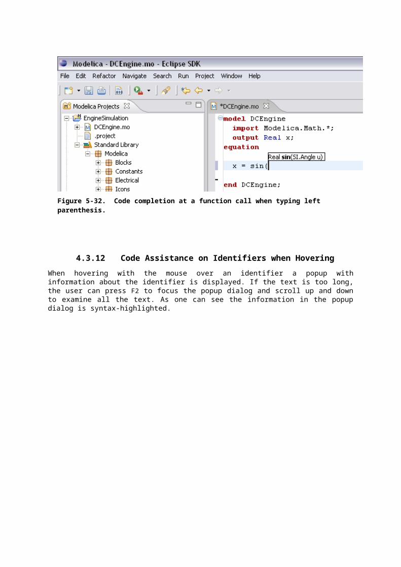
Support for several platforms Linux, MacOS, Windows (2000, Xp, Vista). Support for record and strings as function arguments. Many bug fixes. (Not part of OMC): Additional free graphic editor SimForge can be used with OpenModelica.

A.2.2 OpenModelica Notebook (OMNotebook)A number of improvements, primarily in the plotting functionality and platform availability.

A number of improvements in the plotting functionality: scalable plots, zooming, logarithmic plots, grids, etc.

Programmable plotting accessible through a Modelica API. Simple 3D visualization. Support for several platforms Linux, MacOS, Windows (2000, Xp, Vista).

A.2.3 OpenModelica Shell (OMShell)Same as previously.

A.2.4 OpenModelica Eclipse Plug-in (MDT)Minor bug fixes.

A.2.5 OpenModelica Development Environment (OMDev) Same as previously.

A.3 OpenModelica 1.4.4, Feb 2008This release is primarily a bug fix release, except for a preliminary version of new plotting functionality available both from the OMNotebook and separately through a Modelica API. This is also the first release under the open source license OSMC-PL (Open Source Modelica Consortium Public License), with support from the recently created Open Source Modelica Consortium. An integrated version handler, bug-, and issue tracker has also been added.

A.3.1 OpenModelica Compiler (OMC)This release includes small improvements and some bugfixes of the OpenModelica Compiler (OMC):

Better support for if-equations, also inside when. Better support for calling functions in parameter expressions and interactively through dynamic

loading of functions. Less memory consumtion during compilation and interactive evaluation. A number of bug-fixes.

A.3.2 OpenModelica Notebook (OMNotebook)Test release of improvements, primarily in the plotting functionality and platform availability.

Preliminary version of improvements in the plotting functionality: scalable plots, zooming, logarithmic plots, grids, etc., currently available in a preliminary version through the plot2 function.

Programmable plotting accessible through a Modelica API.

A.3.3 OpenModelica Shell (OMShell)Same as previously.

A.3.4 OpenModelica Eclipse Plug-in (MDT)This release includes minor bugfixes of MDT and the associated MetaModelica debugger:

A.3.5 OpenModelica Development Environment (OMDev) Extended test suite with a better structure. Version handling, bug tracking, issue tracking, etc. now available under the integrated Codebeamer

A.4 OpenModelica 1.4.3, June 2007This release has a number of significant improvements of the OMC compiler, OMNotebook, the MDT plugin and the OMDev. Increased platform availability now also for Linux and Macintosh, in addition to Windows. OMShell is the same as previously, but now ported to Linux and Mac.

A.4.1 OpenModelica Compiler (OMC)This release includes a number of improvements of the OpenModelica Compiler (OMC):

Significantly increased compilation speed, especially with large models and many packages. Now available also for Linux and Macintosh platforms. Support for when-equations in algorithm sections, including elsewhen. Support for inner/outer prefixes of components (but without type error checking). Improved solution of nonlinear systems. Added ability to compile generated simulation code using Visual Studio compiler. Added "smart setting of fixed attribute to false. If initial equations, OMC instead has fixed=true as

default for states due to allowing overdetermined initial equation systems. Better state select heuristics. New function getIncidenceMatrix(ClassName) for dumping the incidence matrix. Builtin functions String(), product(), ndims(), implemented. Support for terminate() and assert() in equations. In emitted flat form: protected variables are now prefixed with protected when printing flat class. Some support for tables, using omcTableTimeIni instead of dymTableTimeIni2. Better support for empty arrays, and support for matrix operations like a*[1,2;3,4]. Improved val() function can now evaluate array elements and record fields, e.g. val(x[n]), val(x.y) . Support for reinit in algorithm sections. String support in external functions. Double precision floating point precision now also for interpreted expressions Better simulation error messages. Support for der(expressions). Support for iterator expressions such as {3*i for i in 1..10}.

More test cases in the test suite. A number of bug fixes, including sample and event handling bugs.

A.4.2 OpenModelica Notebook (OMNotebook)A number of improvements, primarily in the platform availability.

Available on the Linux and Macintosh platforms, in addition to Windows. Fixed cell copying bugs, plotting of derivatives now works, etc.

A.4.3 OpenModelica Shell (OMShell)Now available also on the Macintosh platform.

A.4.4 OpenModelica Eclipse Plug-in (MDT)This release includes major improvements of MDT and the associated MetaModelica debugger:

Greatly improved browsing and code completion works both for standard Modelica and for MetaModelica.

Hovering over identifiers displays type information. A new and greatly improved implementation of the debugger for MetaModelica algorithmic code,

operational in Eclipse. Greatly improved performance – only approx 10% speed reduction even for 100 000 line programs. Greatly improved single stepping, step over, data structure browsing, etc.

Many bug fixes.

A.4.5 OpenModelica Development Environment (OMDev) Increased compilation speed for MetaModelica. Better if-expression support in MetaModelica.

A.5 OpenModelica 1.4.2, October 2006This release has improvements and bug fixes of the OMC compiler, OMNotebook, the MDT plugin and the OMDev. OMShell is the same as previously.

A.5.1 OpenModelica Compiler (OMC)This release includes further improvements of the OpenModelica Compiler (OMC):

Improved initialization and index reduction. Support for integer arrays is now largely implemented. The val(variable,time) scripting function for accessing the value of a simulation result variable at a

certain point in the simulated time. Interactive evalution of for-loops, while-loops, if-statements, if-expressions, in the interactive

scripting mode. Improved documentation and examples of calling the Model Query and Manipulation API. Many bug fixes.

A.5.2 OpenModelica Notebook (OMNotebook)

Search and replace functions have been added. The DrModelica tutorial (all files) has been updated, obsolete sections removed, and models which are not supported by the current implementation marked clearly. Automatic recognition of the .onb suffix (e.g. when double-clicking) in Windows makes it even more convenient to use.

A.5.3 OpenModelica Eclipse Plug-in (MDT)Two major improvements are added in this release:

Browsing and code completion works both for standard Modelica and for MetaModelica. The debugger for algorithmic code is now available and operational in Eclipse for debugging of

MetaModelica programs.

A.5.4 OpenModelica Development Environment (OMDev) Mostly the same as previously.

A.6 OpenModelica 1.4.1, June 2006This release has only improvements and bug fixes of the OMC compiler, the MDT plugin and the OMDev components. The OMShell and OMNotebook are the same.

A.6.1 OpenModelica Compiler (OMC)This release includes further improvements of the OpenModelica Compiler (OMC):

Support for external objects. OMC now reports the version number (via command line switches or CORBA API getVersion()). Implemented caching for faster instantiation of large models. Many bug fixes.

A.6.2 OpenModelica Eclipse Plug-in (MDT)Improvements of the error reporting when building the OMC compiler. The errors are now added to the problems view. The latest MDT release is version 0.6.6 (2006-06-06).

A.6.3 OpenModelica Development Environment (OMDev) Small fixes in the MetaModelica compiler. MetaModelica Users Guide is now part of the OMDev release. The latest OMDev was release in 2006-06-06.

A.7 OpenModelica 1.4.0, May 2006This release has a number of improvements described below. The most significant change is probably that OMC has now been translated to an extended subset of Modelica (MetaModelica), and that all development of the compiler is now done in this version..

A.7.1 OpenModelica Compiler (OMC)This release includes further improvements of the OpenModelica Compiler (OMC):

Partial support for mixed system of equations.

New initialization routine, based on optimization (minimizing residuals of initial equations). Symbolic simplification of builtin operators for vectors and matrices. Improved code generation in simulation code to support e.g. Modelica functions. Support for classes extending basic types, e.g. connectors (support for MSL 2.2 block connectors). Support for parametric plotting via the plotParametric command. Many bug fixes.

A.7.2 OpenModelica Shell (OMShell)Essentially the same OMShell as in 1.3.1. One difference is that now all error messages are sent to the command window instead of to a separate log window.

A.7.3 OpenModelica Notebook (OMNotebook)Many significant improvements and bug fixes. This version supports graphic plots within the cells in the notebook. Improved cell handling and Modelica code syntax highlighting. Command completion of the most common OMC commands is now supported. The notebook has been used in several courses.

A.7.4 OpenModelica Eclipse Plug-in (MDT)This is the first really useful version of MDT. Full browsing of Modelica code, e.g. the MSL 2.2, is now supported. (MetaModelica browsing is not yet fully supported). Full support for automatic indentation of Modelica code, including the MetaModelica extensions. Many bug fixes. The Eclipse plug-in is now in use for OpenModelica development at PELAB and MathCore Engineering AB since approximately one month.

A.7.5 OpenModelica Development Environment (OMDev)The following mechanisms have been put in place to support OpenModelica development.

A separate web page for OMDev (OpenModelica Development Environment).

A pre-packaged OMDev zip-file with precompiled binaries for development under Windows using the mingw Gnu compiler from the Eclipse MDT plug-in. (Development is also possible using Visual Studio).

All source code of the OpenModelica compiler has recently been translated to an extended subset of Modelica, currently called MetaModelica. The current size of OMC is approximately 100 000 lines All development is now done in this version.

A new tutorial and users guide for development in MetaModelica. Successful builds and tests of OMC under Linux and Solaris.

A.8 OpenModelica 1.3.1, November 2005This release has several important highlights.

This is also the first release for which the New BSD (Berkeley) open-source license applies to the source code, including the whole compiler and run-time system. This makes is possible to use OpenModelica for both academic and commercial purposes without restrictions.

A.8.1 OpenModelica Compiler (OMC)

This release includes a significantly improved OpenModelica Compiler (OMC):

Support for hybrid and discrete-event simulation (if-equations, if-expressions, when-equations; not yet if-statements and when-statements).

Parsing of full Modelica 2.2 Improved support for external functions. Vectorization of function arguments; each-modifiers, better implementation of replaceable, better

handling of structural parameters, better support for vector and array operations, and many other improvements.

Flattening of the Modelica Block library version 1.5 (except a few models), and simulation of most of these.

Automatic index reduction (present also in previous release). Updated User's Guide including examples of hybrid simulation and external functions.

A.8.2 OpenModelica Shell (OMShell)An improved window-based interactive command shell, now including command completion and better editing and font size support.

A.8.3 OpenModelica Notebook (OMNotebook)A free implementation of an OpenModelica notebook (OMNOtebook), for electronic books with course material, including the DrModelica interactive course material. It is possible to simulate and plot from this notebook.

A.8.4 OpenModelica Eclipse Plug-in (MDT)An early alpha version of the first Eclipse plug-in (called MDT for Modelica Development Tooling) for Modelica Development. This version gives compilation support and partial support for browsing Modelica package hierarchies and classes.

A.8.5 OpenModelica Development Environment (OMDev)The following mechanisms have been put in place to support OpenModelica development.

Bugzilla support for OpenModelica bug tracking, accessible to anybody. A system for automatic regression testing of the compiler and simulator, (+ other system parts)

usually run at check in time. Version handling is done using SVN, which is better than the previously used CVS system. For

example, name change of modules is now possible within the version handling system.

Appendix B

Contributors to OpenModelica

This Appendix lists the individuals who have made significant contributions to OpenModelica, in the form of software development, design, documentation, project leadership, tutorial material, promotion, etc. The individuals are listed for each year, from 1998 to the current year: the project leader and main author/editor of this document followed by main contributors followed by contributors in alphabetical order.

B.1 OpenModelica Contributors 2009Peter Fritzson, PELAB, Linköping University, Linköping, Sweden.

Adrian Pop, PELAB, Linköping University, Linköping, Sweden.Peter Aronsson, MathCore Engineering AB, Linköping, Sweden.

David Akhvlediani, PELAB, Linköping University, Linköping, Sweden.Bernhard Bachmann, Fachhochschule Bielefeld, Bielefeld, Germany.Vasile Baluta, PELAB, Linköping University, Linköping, Sweden.Constantin Belyaev, Bashpromavtomatika Ltd., Ufa, RussiaSimon Björklén, PELAB, Linköping University, Linköping, Sweden.Mikael Blom, PELAB, Linköping University, Linköping, Sweden.Willi Braun, Fachhochschule Bielefeld, Bielefeld, Germany.David Broman, PELAB, Linköping University, Linköping, Sweden.Stefan Brus, PELAB, Linköping University, Linköping, Sweden.Francesco Casella, Politecnico di Milano, Milan, ItalyFilippo Donida, Politecnico di Milano, Milan, ItalyHenrik Eriksson, PELAB, Linköping University, Linköping, Sweden.Anders Fernström, PELAB, Linköping University, Linköping, Sweden.Jens Frenkel, TU Dresden, Dresden, Germany.Pavel Grozman, Equa AB, Stockholm, Sweden.Michael Hanke, NADA, KTH, StockholmDaniel Hedberg, MathCore Engineering AB, Linköping, Sweden.Alf Isaksson, ABB Corporate Research, Västerås, SwedenKim Jansson, PELAB, Linköping University, Linköping, Sweden.Daniel Kanth, Bosch-Rexroth, Lohr am Main, GermanyTommi Karhela, VTT, Espoo, Finland.Joel Klinghed, PELAB, Linköping University, Linköping, Sweden.Juha Kortelainen, VTT, Espoo, FinlandAlexey Lebedev, Equa Simulation AB, Stockholm, SwedenMagnus Leksell, Linköping, SwedenOliver Lenord, Bosch-Rexroth, Lohr am Main, GermanyHåkan Lundvall, PELAB, Linköping University, Linköping, Sweden.Henrik Magnusson, Linköping, SwedenEric Meyers, Pratt & Whitney Rocketdyne, Palm City, Florida, USA.Hannu Niemistö, VTT, Espoo, FinlandKristoffer Norling, PELAB, Linköping University, Linköping, Sweden.

Atanas Pavlov, Munich, Germany.Pavol Privitzer, Institute of Pathological Physiology, Praha, Czech Republic.Per Sahlin, Equa Simulation AB, Stockholm, Sweden.Gerhard Schmitz, University of Hamburg, Hamburg, GermanyKlas Sjöholm, PELAB, Linköping University, Linköping, Sweden.Martin Sjölund, PELAB, Linköping University, Linköping, Sweden.Kristian Stavåker, PELAB, Linköping University, Linköping, Sweden.Mohsen Torabzadeh-Tari, PELAB, Linköping University, Linköping, Sweden.Niklas Worschech, Bosch-Rexroth, Lohr am Main, GermanyRobert Wotzlaw, Goettingen, GermanyBjörn Zachrisson, MathCore Engineering AB, Linköping, Sweden

B.2 OpenModelica Contributors 2008Peter Fritzson, PELAB, Linköping University, Linköping, Sweden.

Adrian Pop, PELAB, Linköping University, Linköping, Sweden.Peter Aronsson, MathCore Engineering AB, Linköping, Sweden.

David Akhvlediani, PELAB, Linköping University, Linköping, Sweden.Bernhard Bachmann, Fachhochschule Bielefeld, Bielefeld, Germany.Vasile Baluta, PELAB, Linköping University, Linköping, Sweden.Mikael Blom, PELAB, Linköping University, Linköping, Sweden.David Broman, PELAB, Linköping University, Linköping, Sweden.Henrik Eriksson, PELAB, Linköping University, Linköping, Sweden.Anders Fernström, PELAB, Linköping University, Linköping, Sweden.Pavel Grozman, Equa AB, Stockholm, Sweden.Daniel Hedberg, MathCore Engineering AB, Linköping, Sweden.Kim Jansson, PELAB, Linköping University, Linköping, Sweden.Joel Klinghed, PELAB, Linköping University, Linköping, Sweden.Håkan Lundvall, PELAB, Linköping University, Linköping, Sweden.Eric Meyers, Pratt & Whitney Rocketdyne, Palm City, Florida, USA.Kristoffer Norling, PELAB, Linköping University, Linköping, Sweden.Anders Sandholm, PELAB, Linköping University, Linköping, Sweden.Klas Sjöholm, PELAB, Linköping University, Linköping, Sweden.Kristian Stavåker, PELAB, Linköping University, Linköping, Sweden.Simon Bjorklén, PELAB, Linköping University, Linköping, Sweden.Constantin Belyaev, Bashpromavtomatika Ltd., Ufa, Russia

B.3 OpenModelica Contributors 2007Peter Fritzson, PELAB, Linköping University, Linköping, Sweden.

Adrian Pop, PELAB, Linköping University, Linköping, Sweden.Peter Aronsson, MathCore Engineering AB, Linköping, Sweden.

David Akhvlediani, PELAB, Linköping University, Linköping, Sweden.Bernhard Bachmann, Fachhochschule Bielefeld, Bielefeld, Germany.David Broman, PELAB, Linköping University, Linköping, Sweden.Henrik Eriksson, PELAB, Linköping University, Linköping, Sweden.Anders Fernström, PELAB, Linköping University, Linköping, Sweden.Pavel Grozman, Equa AB, Stockholm, Sweden.Daniel Hedberg, MathCore Engineering AB, Linköping, Sweden.

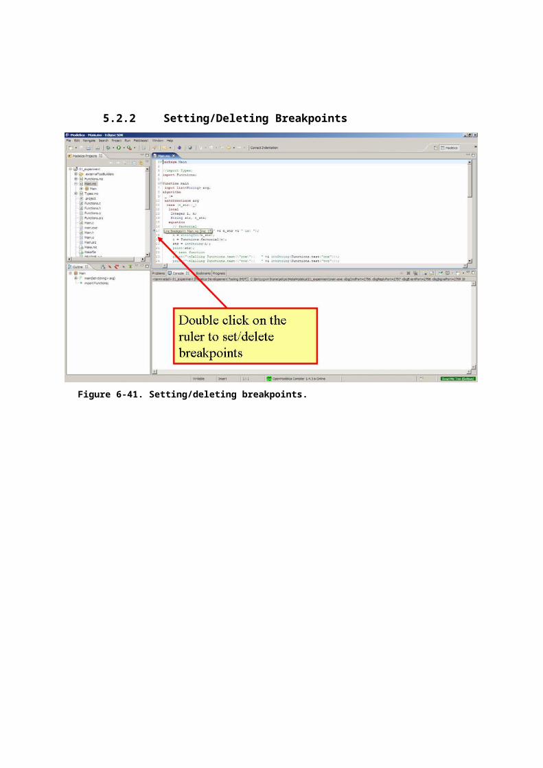
Ola Leifler, IDA, Linköping University, Linköping, Sweden.Håkan Lundvall, PELAB, Linköping University, Linköping, Sweden.Eric Meyers, Pratt & Whitney Rocketdyne, Palm City, Florida, USA.Kristoffer Norling, PELAB, Linköping University, Linköping, Sweden.Anders Sandholm, PELAB, Linköping University, Linköping, Sweden.Klas Sjöholm, PELAB, Linköping University, Linköping, Sweden.William Spinelli, Politecnico di Milano, Milano, ItalyKristian Stavåker, PELAB, Linköping University, Linköping, Sweden.Stefan Vorkoetter, MapleSoft, Waterloo, Canada.Björn Zachrisson, MathCore Engineering AB, Linköping, Sweden.Constantin Belyaev, Bashpromavtomatika Ltd., Ufa, Russia

B.4 OpenModelica Contributors 2006Peter Fritzson, PELAB, Linköping University, Linköping, Sweden.

Peter Aronsson, MathCore Engineering AB, Linköping, Sweden.Adrian Pop, PELAB, Linköping University, Linköping, Sweden.

David Akhvlediani, PELAB, Linköping University, Linköping, Sweden.Bernhard Bachmann, Fachhochschule Bielefeld, Bielefeld, Germany.David Broman, PELAB, Linköping University, Linköping, Sweden.Anders Fernström, PELAB, Linköping University, Linköping, Sweden.Elmir Jagudin, PELAB, Linköping University, Linköping, Sweden.Håkan Lundvall, PELAB, Linköping University, Linköping, Sweden.Kaj Nyström, PELAB, Linköping University, Linköping, Sweden.Lucian Popescu, MathCore Engineering AB, Linköping, Sweden.Andreas Remar, PELAB, Linköping University, Linköping, Sweden.Anders Sandholm, PELAB, Linköping University, Linköping, Sweden.

B.5 OpenModelica Contributors 2005Peter Fritzson, PELAB, Linköping University, Linköping, Sweden.

Peter Aronsson, PELAB, Linköping University and MathCore Engineering AB, Linköping, Sweden.Adrian Pop, PELAB, Linköping University, Linköping, Sweden.Håkan Lundvall, PELAB, Linköping University, Linköping, Sweden.

Ingemar Axelsson, PELAB, Linköping University, Linköping, Sweden.David Broman, PELAB, Linköping University, Linköping, Sweden.Daniel Hedberg, MathCore Engineering AB, Linköping, Sweden.Håkan Lundvall, PELAB, Linköping University, Linköping, Sweden.Kaj Nyström, PELAB, Linköping University, Linköping, Sweden.Lucian Popescu, MathCore Engineering AB, Linköping, Sweden.Levon Saldamli, PELAB, Linköping University, Linköping, Sweden.

B.6 OpenModelica Contributors 2004Peter Fritzson, PELAB, Linköping University, Linköping, Sweden.

Peter Aronsson, Linköping University, Linköping, Sweden.

Bernhard Bachmann, Fachhochschule Bielefeld, Bielefeld, Germany.Peter Bunus, PELAB, Linköping University, Linköping, Sweden.Daniel Hedberg, MathCore Engineering AB, Linköping, Sweden.

Håkan Lundvall, PELAB, Linköping University, Linköping, Sweden.Emma Larsdotter Nilsson, PELAB, Linköping University, Linköping, Sweden.Kaj Nyström, PELAB, Linköping University, Linköping, Sweden.Adrian Pop, PELAB, Linköping University, Linköping, Sweden.Lucian Popescu, MathCore Engineering AB, Linköping, Sweden.Levon Saldamli, PELAB, Linköping University, Linköping, Sweden.

B.7 OpenModelica Contributors 2003Peter Fritzson, PELAB, Linköping University, Linköping, Sweden.

Peter Aronsson, Linköping University, Linköping, Sweden.Levon Saldamli, PELAB, Linköping University, Linköping, Sweden.

Peter Bunus, PELAB, Linköping University, Linköping, Sweden.Vadim Engelson, PELAB, Linköping University, Linköping, Sweden.Daniel Hedberg, Linköping University, Linköping, Sweden.Eva-Lena Lengquist-Sandelin, PELAB, Linköping University, Linköping, Sweden.Susanna Monemar, PELAB, Linköping University, Linköping, Sweden.Adrian Pop, PELAB, Linköping University, Linköping, Sweden.Erik Svensson, MathCore Engineering AB, Linköping, Sweden.

B.8 OpenModelica Contributors 2002Peter Fritzson, PELAB, Linköping University, Linköping, Sweden.

Levon Saldamli, PELAB, Linköping University, Linköping, Sweden.Peter Aronsson, Linköping University, Linköping, Sweden.

Daniel Hedberg, Linköping University, Linköping, Sweden.Henrik Johansson, PELAB, Linköping University, Linköping, SwedenAndreas Karström, PELAB, Linköping University, Linköping, Sweden

B.9 OpenModelica Contributors 2001Peter Fritzson, PELAB, Linköping University, Linköping, Sweden.

Levon Saldamli, PELAB, Linköping University, Linköping, Sweden.

Peter Aronsson, Linköping University, Linköping, Sweden.

B.10 OpenModelica Contributors 2000Peter Fritzson, PELAB, Linköping University, Linköping, Sweden.

B.11 OpenModelica Contributors 1999Peter Fritzson, PELAB, Linköping University, Linköping, Sweden

–

Peter Rönnquist, PELAB, Linköping University, Linköping, Sweden.

B.12 OpenModelica Contributors 1998Peter Fritzson, PELAB, Linköping University, Linköping, Sweden.

David Kågedal, PELAB, Linköping University, Linköping, Sweden.

Vadim Engelson, PELAB, Linköping University, Linköping, Sweden.

Index

literate programming...........................49