Viewing - cs.usfca.edu
55
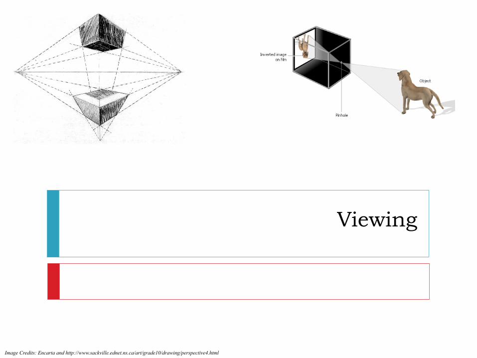
Viewing Image Credits: Encarta and http://www.sackville.ednet.ns.ca/art/grade10/drawing/perspective4.html
Transcript of Viewing - cs.usfca.edu
Viewing
Image Credits: Encarta and http://www.sackville.ednet.ns.ca/art/grade10/drawing/perspective4.html
Graphics Pipeline
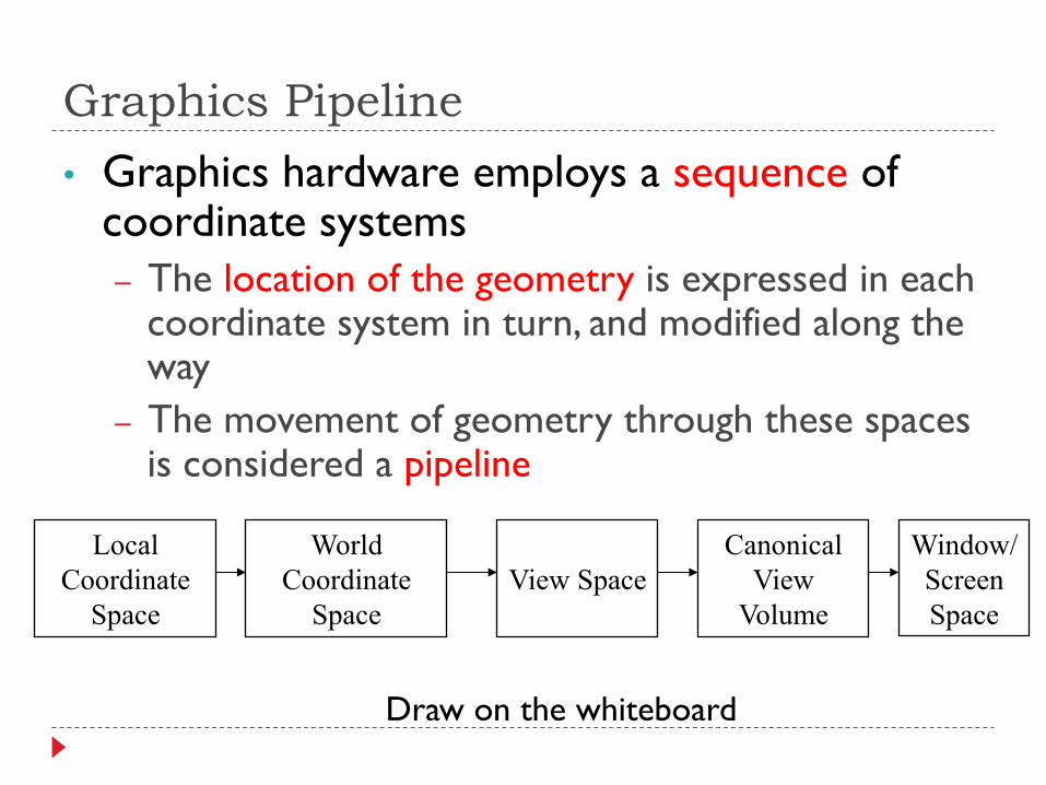
• Graphics hardware employs a sequence of coordinate systems – The location of the geometry is expressed in each
coordinate system in turn, and modified along the way
– The movement of geometry through these spaces is considered a pipeline
Local Coordinate
Space
World Coordinate
Space
View Space
Canonical View
Volume
Window/Screen Space
Draw on the whiteboard
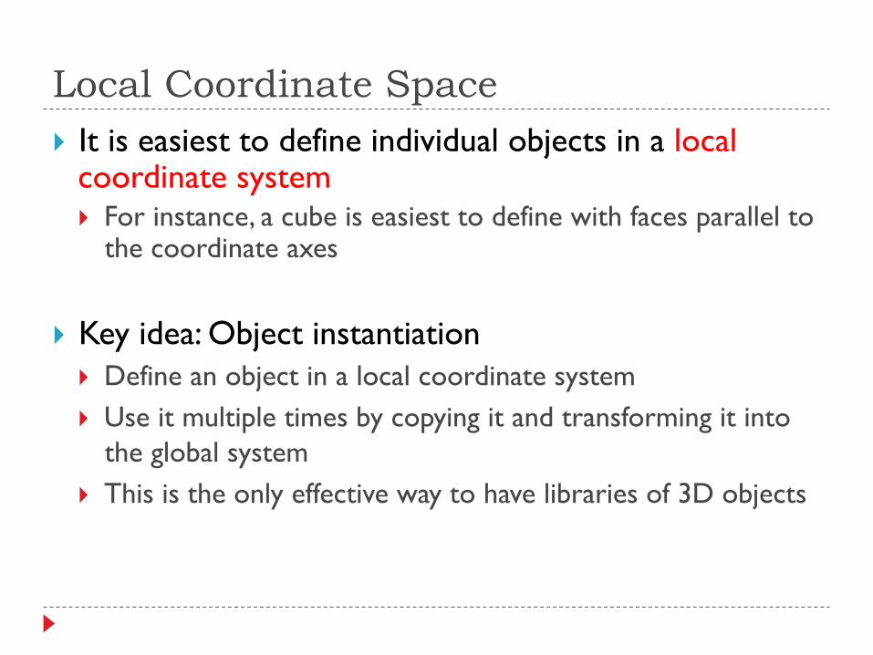
Local Coordinate Space } It is easiest to define individual objects in a local
coordinate system } For instance, a cube is easiest to define with faces parallel to
the coordinate axes
} Key idea: Object instantiation } Define an object in a local coordinate system } Use it multiple times by copying it and transforming it into
the global system } This is the only effective way to have libraries of 3D objects
World Coordinate System } Everything in the world is transformed into one
coordinate system - the world coordinate system } It has an origin, and three coordinate directions, x, y, and z
} Lighting is defined in this space } The locations, brightness’ and types of lights
} The camera is defined with respect to this space
} Some higher level operations, such as advanced visibility computations, can be done here
View Space } Define a coordinate system based on the eye and
image plane – the camera } The eye is the center of projection, like the aperture in a
camera } The image plane is the orientation of the plane on which the
image should “appear,” like the film plane of a camera } Some camera parameters are easiest to define in this
space } Focal length, image size
} Relative depth is captured by a single number in this space } The “normal to image plane” coordinate
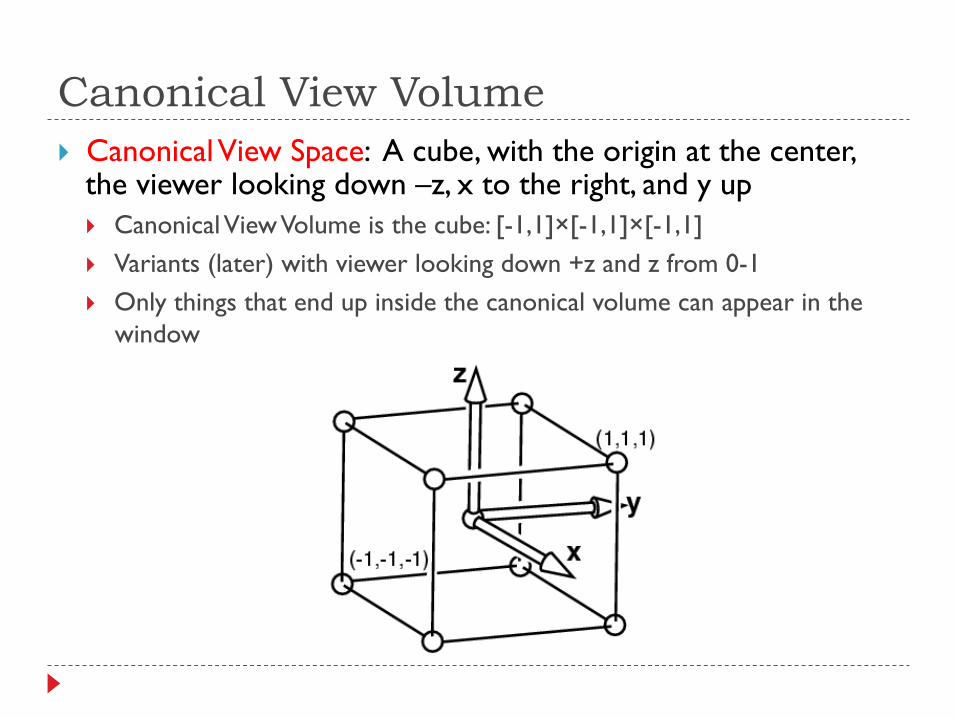
Canonical View Volume } Canonical View Space: A cube, with the origin at the center,
the viewer looking down –z, x to the right, and y up } Canonical View Volume is the cube: [-1,1]×[-1,1]×[-1,1] } Variants (later) with viewer looking down +z and z from 0-1 } Only things that end up inside the canonical volume can appear in the
window
Canonical View Volume } Tasks: Parallel sides and unit dimensions make many
operations easier } Clipping – decide what is in the window } Rasterization - decide which pixels are covered } Hidden surface removal - decide what is in front } Shading - decide what color things are
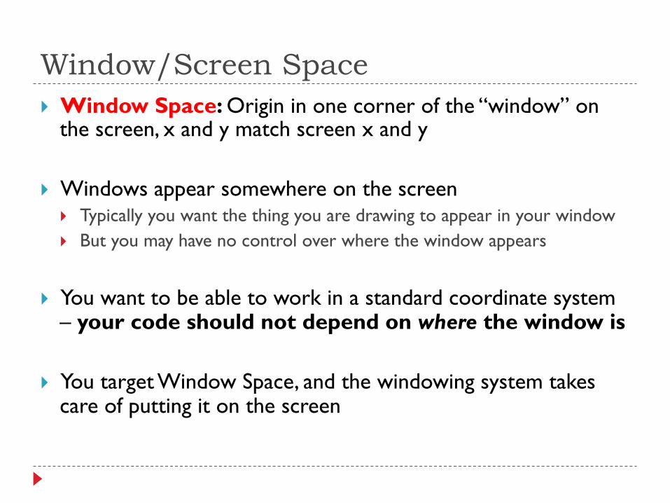
Window/Screen Space } Window Space: Origin in one corner of the “window” on
the screen, x and y match screen x and y
} Windows appear somewhere on the screen } Typically you want the thing you are drawing to appear in your window } But you may have no control over where the window appears
} You want to be able to work in a standard coordinate system – your code should not depend on where the window is
} You target Window Space, and the windowing system takes care of putting it on the screen
Canonical → Window Transform
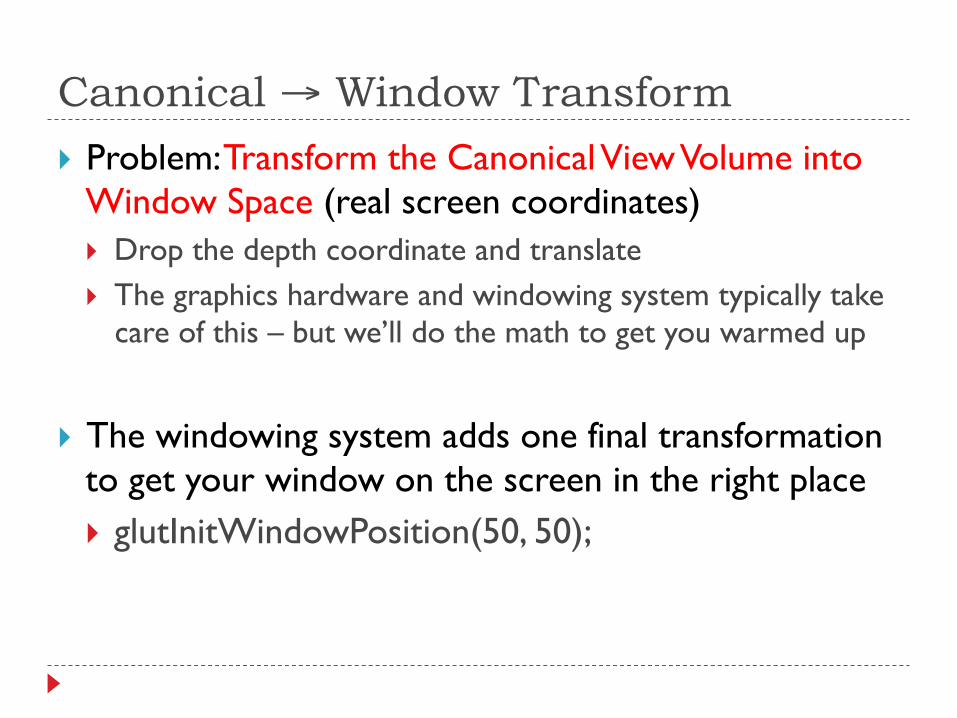
} Problem: Transform the Canonical View Volume into Window Space (real screen coordinates) } Drop the depth coordinate and translate } The graphics hardware and windowing system typically take
care of this – but we’ll do the math to get you warmed up
} The windowing system adds one final transformation to get your window on the screen in the right place } glutInitWindowPosition(50, 50);
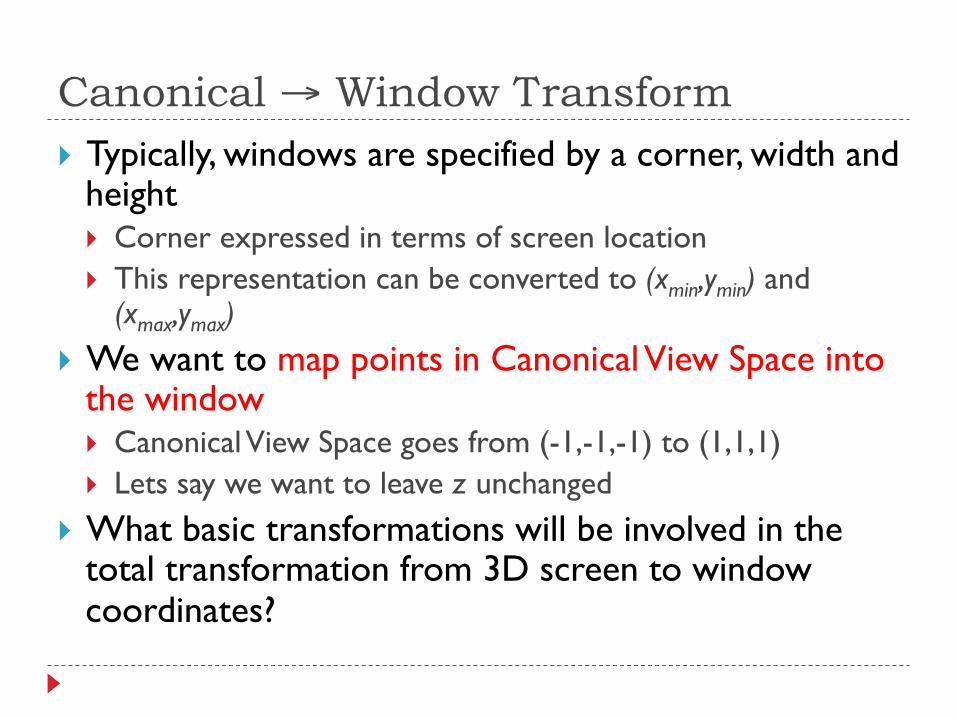
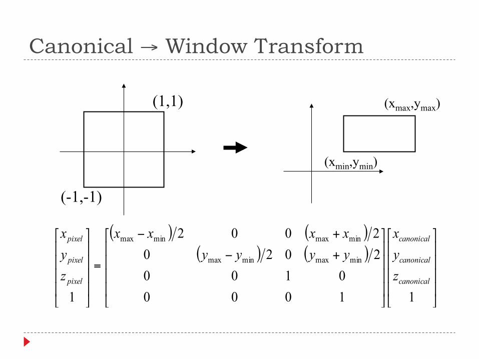
Canonical → Window Transform } Typically, windows are specified by a corner, width and
height } Corner expressed in terms of screen location } This representation can be converted to (xmin,ymin) and
(xmax,ymax) } We want to map points in Canonical View Space into
the window } Canonical View Space goes from (-1,-1,-1) to (1,1,1) } Lets say we want to leave z unchanged
} What basic transformations will be involved in the total transformation from 3D screen to window coordinates?
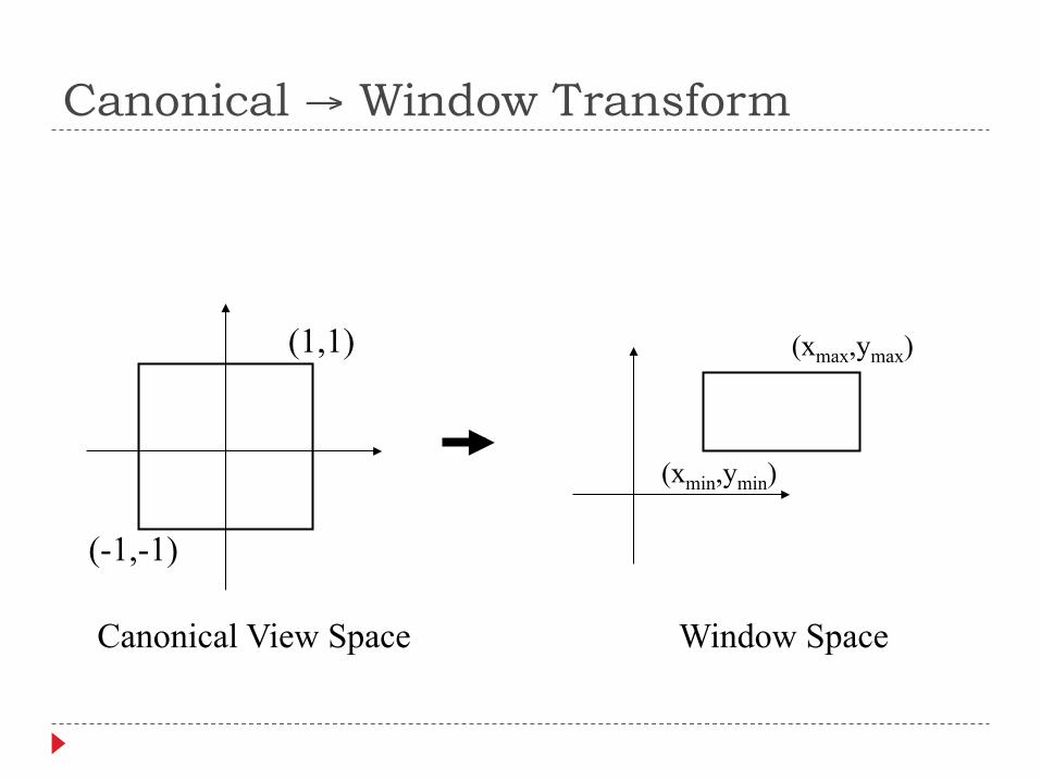
(-1,-1)
(1,1)
(xmin,ymin)
(xmax,ymax)
Canonical View Space Window Space
Canonical → Window Transform
(-1,-1)
(1,1)
(xmin,ymin)
(xmax,ymax)
( ) ( )( ) ( )
⎥⎥⎥⎥
⎦
⎤
⎢⎢⎢⎢
⎣
⎡
⎥⎥⎥⎥
⎦
⎤
⎢⎢⎢⎢
⎣
⎡
+−
+−
=
⎥⎥⎥⎥
⎦
⎤
⎢⎢⎢⎢
⎣
⎡
110000100
20202002
1
minmaxminmax
minmaxminmax
canonical
canonical
canonical
pixel
pixel
pixel
zyx
yyyyxxxx
zyx
Canonical → Window Transform
Canonical → Window Transform } You almost never have to worry about the canonical to
window transform
} In OpenGL, you tell it which part of your window to draw in – relative to the window’s coordinates } That is, you tell it where to put the canonical view volume } You must do this whenever the window changes size } Window (not the screen) has origin at bottom left } glViewport(minx, miny, maxx, maxy) } Typically: glViewport(0, 0, width, height)fills the entire
window with the image } Why might you not fill the entire window?
View Volumes } Only stuff inside the Canonical View Volume gets drawn
} The window is of finite size, and we can only store a finite number of pixels
} We can only store a discrete, finite range of depths } Like color, only have a fixed number of bits at each pixel
} Points too close or too far away will not be drawn } But, it is inconvenient to model the world as a unit box
} A view volume is the region of space we wish to transform into the Canonical View Volume for drawing } Only stuff inside the view volume gets drawn } Describing the view volume is a major part of defining the view
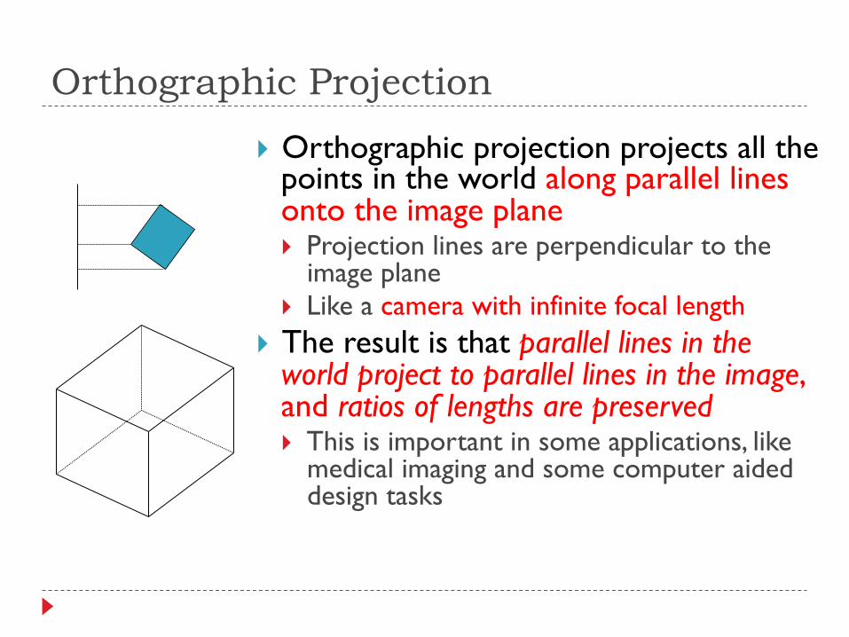
Orthographic Projection
} Orthographic projection projects all the points in the world along parallel lines onto the image plane } Projection lines are perpendicular to the
image plane } Like a camera with infinite focal length
} The result is that parallel lines in the world project to parallel lines in the image, and ratios of lengths are preserved } This is important in some applications, like
medical imaging and some computer aided design tasks
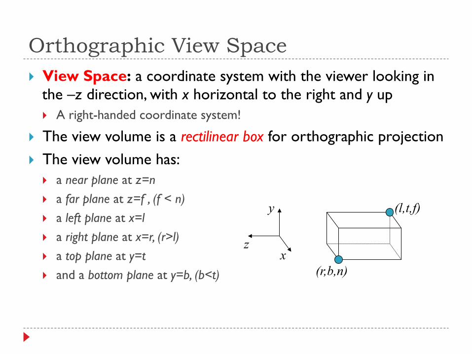
Orthographic View Space } View Space: a coordinate system with the viewer looking in
the –z direction, with x horizontal to the right and y up } A right-handed coordinate system!
} The view volume is a rectilinear box for orthographic projection } The view volume has:
} a near plane at z=n } a far plane at z=f , (f < n) } a left plane at x=l } a right plane at x=r, (r>l) } a top plane at y=t } and a bottom plane at y=b, (b<t)
z
y
x (r,b,n)
(l,t,f)
Rendering the Volume } To find out where points end up on the screen, we must
transform View Space into Canonical View Space } We know how to draw Canonical View Space on the screen
} This transformation is “projection” } The mapping looks similar to the one for Canonical to
Window …
( )( )
( )
( )( )( )
( ) ( ) ( )( ) ( ) ( )
( ) ( ) ( )
viewcanonicalviewcanonical
view
view
view
view
view
view
canonical
canonical
canonical
zyx
fnfnfnbtbtbtlrlrlr
zyx
fnbtlr
fnbt
lr
zyx
xMx >−=
⎥⎥⎥⎥
⎦
⎤
⎢⎢⎢⎢
⎣
⎡
⎥⎥⎥⎥
⎦
⎤
⎢⎢⎢⎢
⎣
⎡
−+−−
−+−−
−+−−
=
⎥⎥⎥⎥
⎦
⎤
⎢⎢⎢⎢
⎣
⎡
⎥⎥⎥⎥
⎦
⎤
⎢⎢⎢⎢
⎣
⎡
+−
+−
+−
⎥⎥⎥⎥
⎦
⎤
⎢⎢⎢⎢
⎣
⎡
−
−
−
=
⎥⎥⎥⎥
⎦
⎤
⎢⎢⎢⎢
⎣
⎡
11000200020002
11000210020102001
1000020000200002
1
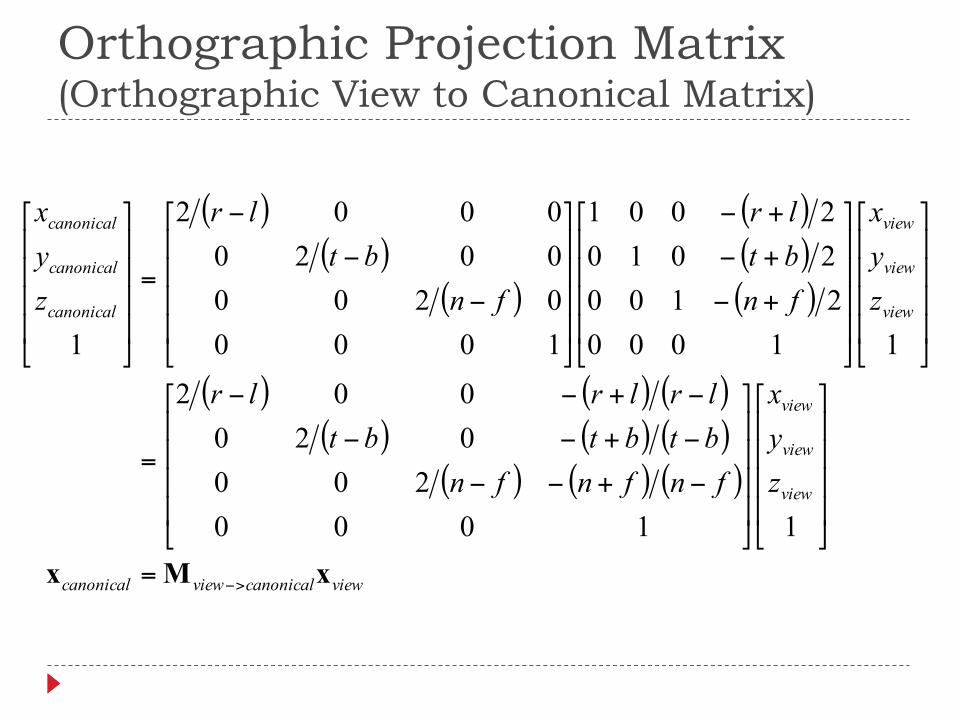
Orthographic Projection Matrix (Orthographic View to Canonical Matrix)
Defining Cameras } View Space is the camera’s local coordinates
} The camera is in some location (eye position) } The camera is looking in some direction (gaze direction) } It is tilted in some orientation (up vector)
} It is inconvenient to model everything in terms of View Space } Biggest problem is that the camera might be moving – we don’t want to
have to explicitly move every object too
} We specify the camera, and hence View Space, with respect to World Space } How can we specify the camera?
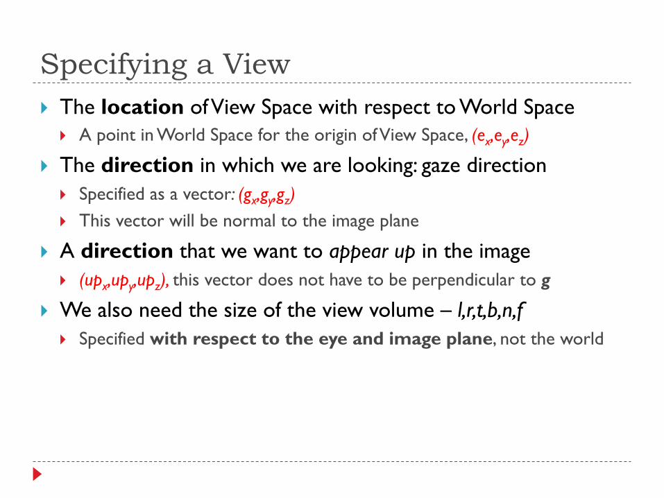
Specifying a View } The location of View Space with respect to World Space
} A point in World Space for the origin of View Space, (ex,ey,ez)
} The direction in which we are looking: gaze direction } Specified as a vector: (gx,gy,gz) } This vector will be normal to the image plane
} A direction that we want to appear up in the image } (upx,upy,upz), this vector does not have to be perpendicular to g
} We also need the size of the view volume – l,r,t,b,n,f } Specified with respect to the eye and image plane, not the world
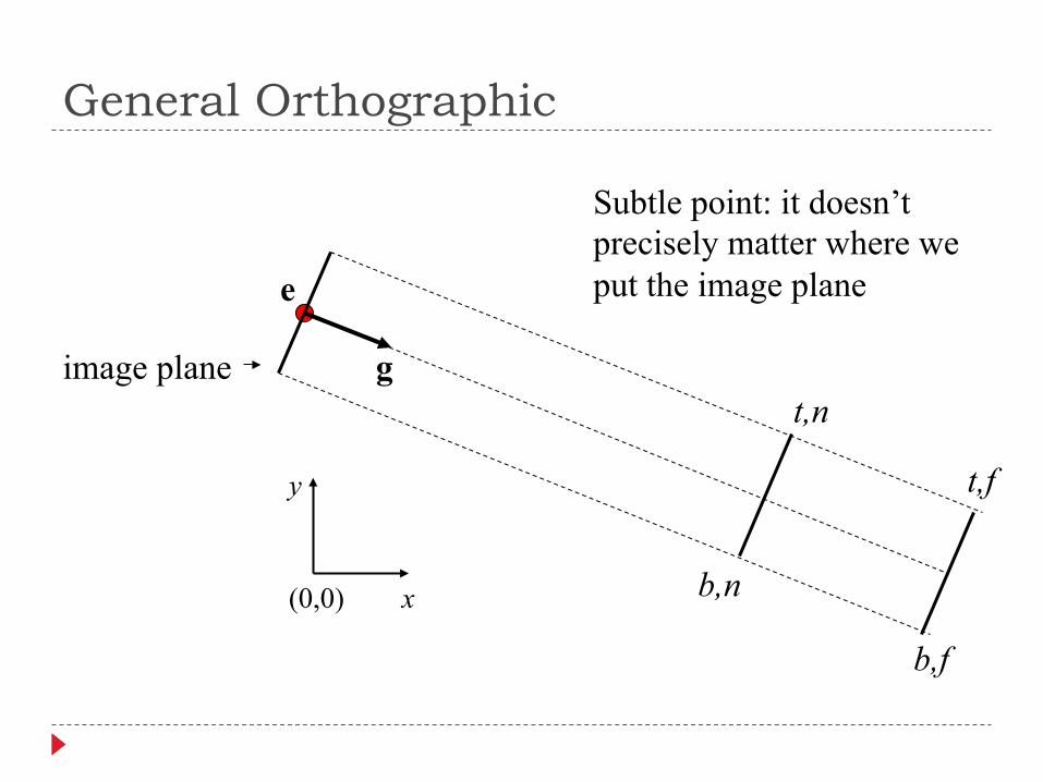
(0,0) x
y
e
image plane g
b,n
b,f
t,n
t,f
Subtle point: it doesn’t precisely matter where we put the image plane
General Orthographic
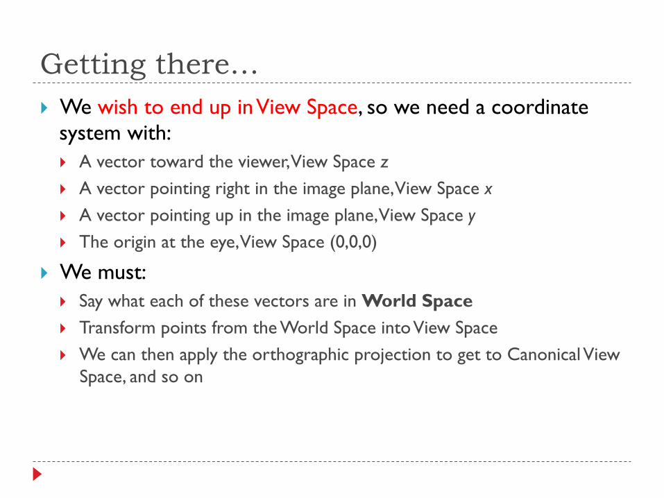
Getting there… } We wish to end up in View Space, so we need a coordinate
system with: } A vector toward the viewer, View Space z } A vector pointing right in the image plane, View Space x } A vector pointing up in the image plane, View Space y } The origin at the eye, View Space (0,0,0)
} We must: } Say what each of these vectors are in World Space } Transform points from the World Space into View Space } We can then apply the orthographic projection to get to Canonical View
Space, and so on
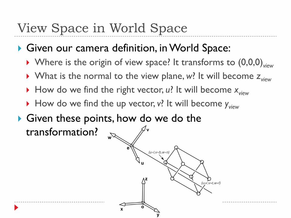
View Space in World Space
} Given our camera definition, in World Space: } Where is the origin of view space? It transforms to (0,0,0)view
} What is the normal to the view plane, w? It will become zview
} How do we find the right vector, u? It will become xview } How do we find the up vector, v? It will become yview
} Given these points, how do we do the transformation?
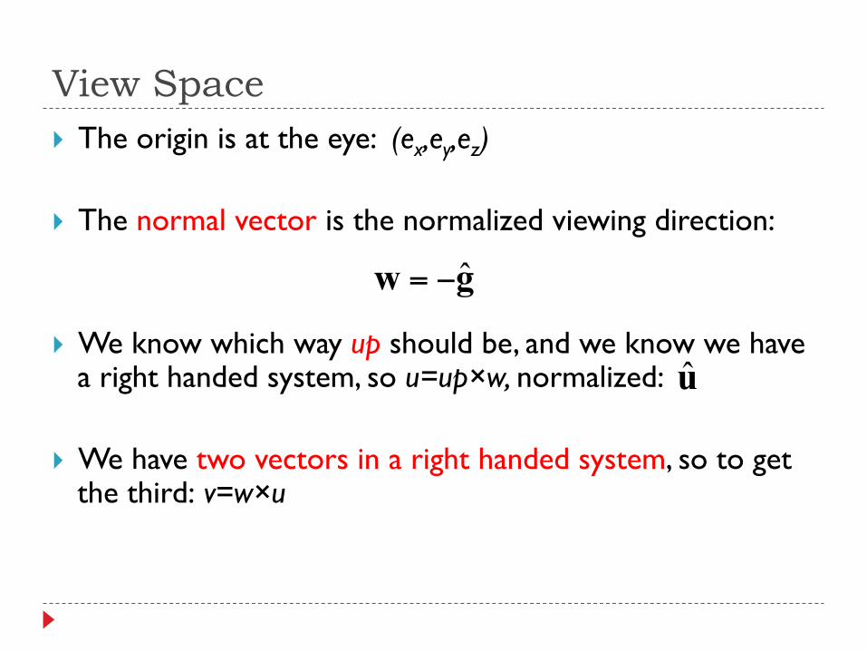
View Space } The origin is at the eye: (ex,ey,ez)
} The normal vector is the normalized viewing direction:
} We know which way up should be, and we know we have a right handed system, so u=up×w, normalized:
} We have two vectors in a right handed system, so to get the third: v=w×u
gw ˆ−=
u
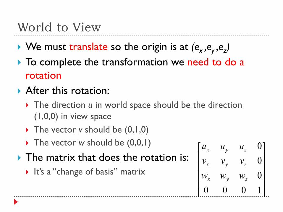
World to View
} We must translate so the origin is at (ex ,ey ,ez) } To complete the transformation we need to do a
rotation } After this rotation:
} The direction u in world space should be the direction (1,0,0) in view space
} The vector v should be (0,1,0) } The vector w should be (0,0,1)
} The matrix that does the rotation is: } It’s a “change of basis” matrix
⎥⎥⎥⎥
⎦
⎤
⎢⎢⎢⎢
⎣
⎡
1000000
zyx
zyx
zyx
wwwvvvuuu
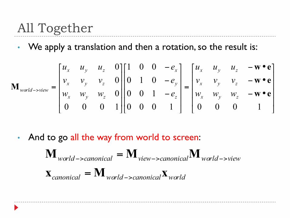
All Together • We apply a translation and then a rotation, so the result is:
• And to go all the way from world to screen:
⎥⎥⎥⎥
⎦
⎤
⎢⎢⎢⎢
⎣
⎡
•−
•−
•−
=
⎥⎥⎥⎥
⎦
⎤
⎢⎢⎢⎢
⎣
⎡
−
−
−
⎥⎥⎥⎥
⎦
⎤
⎢⎢⎢⎢
⎣
⎡
=>−
10001000100010001
1000000
ewewew
Mzyx
zyx
zyx
z
y
x
zyx
zyx
zyx
viewworld wwwvvvuuu
eee
wwwvvvuuu
worldcanonicalworldcanonical
viewworldcanonicalviewcanonicalworld
xMxMMM
>−
>−>−>−
=
=
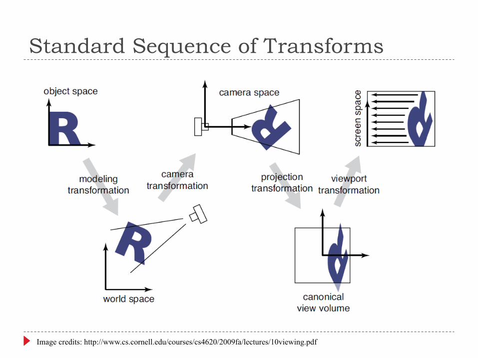
Standard Sequence of Transforms
Image credits: http://www.cs.cornell.edu/courses/cs4620/2009fa/lectures/10viewing.pdf
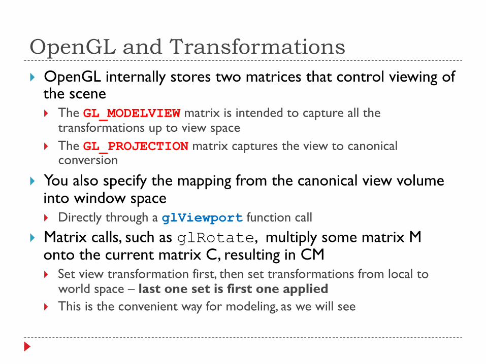
OpenGL and Transformations } OpenGL internally stores two matrices that control viewing of
the scene } The GL_MODELVIEW matrix is intended to capture all the
transformations up to view space } The GL_PROJECTION matrix captures the view to canonical
conversion
} You also specify the mapping from the canonical view volume into window space } Directly through a glViewport function call
} Matrix calls, such as glRotate, multiply some matrix M onto the current matrix C, resulting in CM } Set view transformation first, then set transformations from local to
world space – last one set is first one applied } This is the convenient way for modeling, as we will see
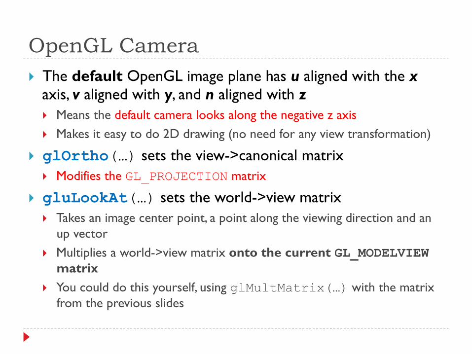
OpenGL Camera } The default OpenGL image plane has u aligned with the x
axis, v aligned with y, and n aligned with z } Means the default camera looks along the negative z axis } Makes it easy to do 2D drawing (no need for any view transformation)
} glOrtho(…) sets the view->canonical matrix } Modifies the GL_PROJECTION matrix
} gluLookAt(…) sets the world->view matrix } Takes an image center point, a point along the viewing direction and an
up vector } Multiplies a world->view matrix onto the current GL_MODELVIEW
matrix } You could do this yourself, using glMultMatrix(…) with the matrix
from the previous slides
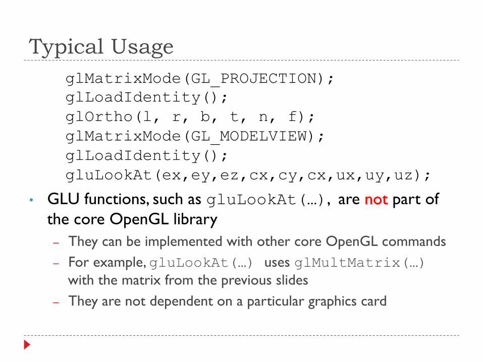
Typical Usage
• GLU functions, such as gluLookAt(…), are not part of the core OpenGL library – They can be implemented with other core OpenGL commands – For example, gluLookAt(…) uses glMultMatrix(…)
with the matrix from the previous slides – They are not dependent on a particular graphics card
glMatrixMode(GL_PROJECTION); glLoadIdentity(); glOrtho(l, r, b, t, n, f); glMatrixMode(GL_MODELVIEW); glLoadIdentity(); gluLookAt(ex,ey,ez,cx,cy,cx,ux,uy,uz);
Demo Tutors/Projection
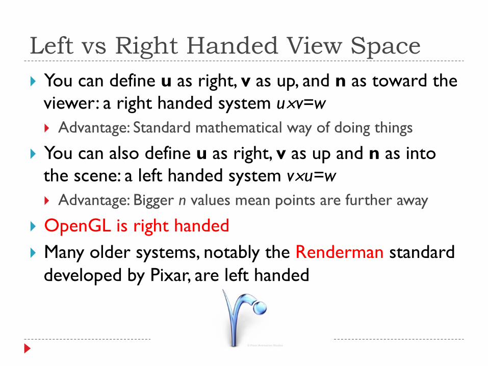
Left vs Right Handed View Space } You can define u as right, v as up, and n as toward the
viewer: a right handed system u×v=w } Advantage: Standard mathematical way of doing things
} You can also define u as right, v as up and n as into the scene: a left handed system v×u=w } Advantage: Bigger n values mean points are further away
} OpenGL is right handed } Many older systems, notably the Renderman standard
developed by Pixar, are left handed
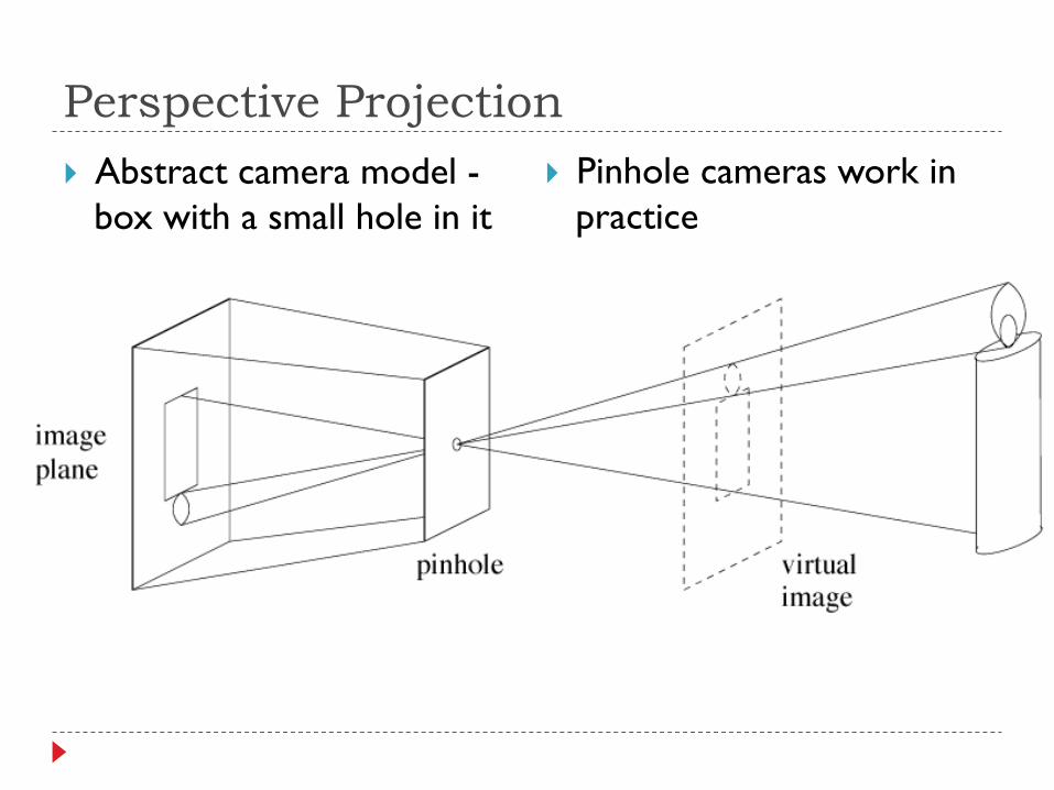
} Pinhole cameras work in practice
Perspective Projection } Abstract camera model -
box with a small hole in it
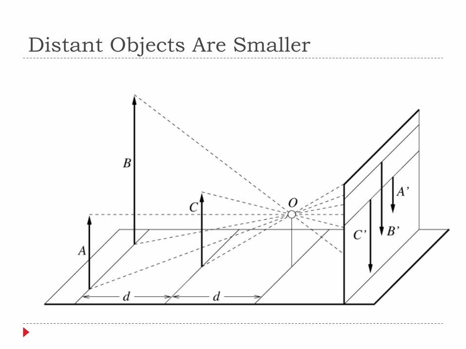
Distant Objects Are Smaller
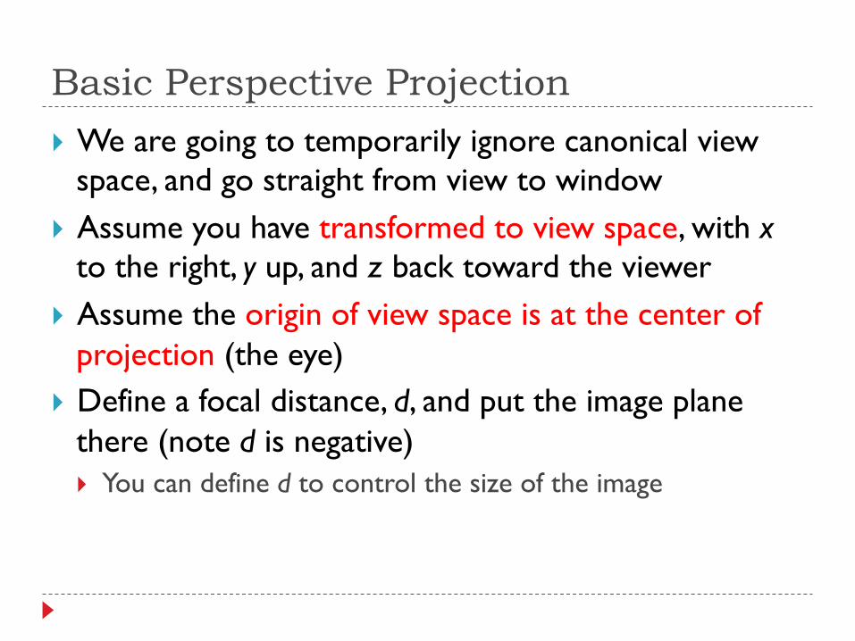
Basic Perspective Projection
} We are going to temporarily ignore canonical view space, and go straight from view to window
} Assume you have transformed to view space, with x to the right, y up, and z back toward the viewer
} Assume the origin of view space is at the center of projection (the eye)
} Define a focal distance, d, and put the image plane there (note d is negative) } You can define d to control the size of the image
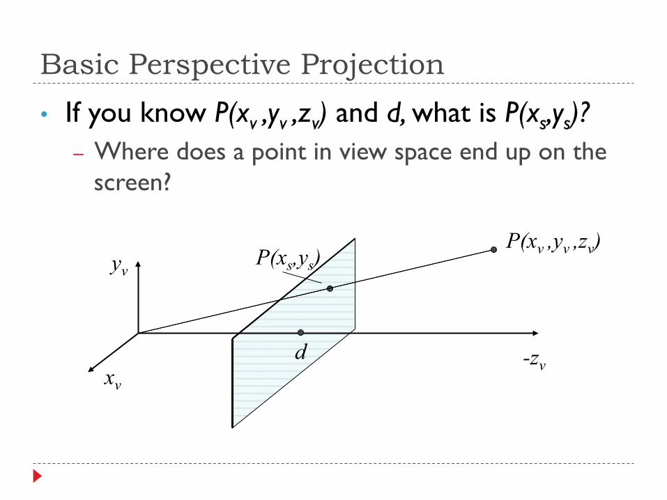
• If you know P(xv ,yv ,zv) and d, what is P(xs,ys)? – Where does a point in view space end up on the
screen?
xv
yv
-zv d
P(xv ,yv ,zv) P(xs,ys)
Basic Perspective Projection
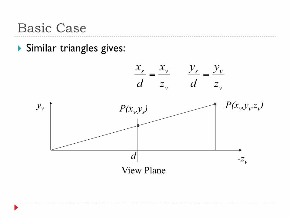
} Similar triangles gives:
v
vs
zx
dx=
v
vs
zy
dy=
yv
-zv
P(xv,yv,zv) P(xs,ys)
View Plane d
Basic Case
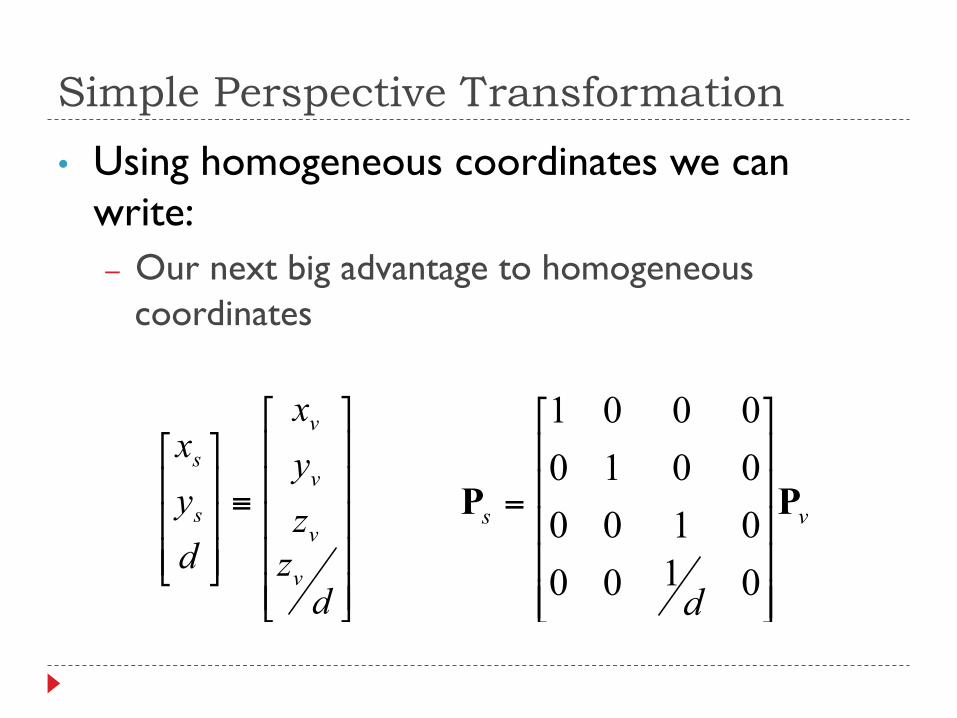
• Using homogeneous coordinates we can write: – Our next big advantage to homogeneous
coordinates
⎥⎥⎥⎥⎥
⎦
⎤
⎢⎢⎢⎢⎢
⎣
⎡
≡
⎥⎥⎥
⎦
⎤
⎢⎢⎢
⎣
⎡
dzzyx
dyx
v
v
v
v
s
s
vs
d
PP
⎥⎥⎥⎥⎥
⎦
⎤
⎢⎢⎢⎢⎢
⎣
⎡
=
0100010000100001
Simple Perspective Transformation
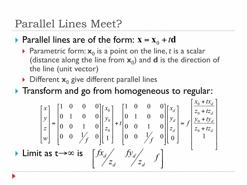
Parallel Lines Meet? } Parallel lines are of the form:
} Parametric form: x0 is a point on the line, t is a scalar (distance along the line from x0) and d is the direction of the line (unit vector)
} Different x0 give different parallel lines } Transform and go from homogeneous to regular:
} Limit as t→∞ is
dxx t+= 0
⎥⎥⎥⎥⎥⎥
⎦
⎤
⎢⎢⎢⎢⎢⎢
⎣
⎡
+
++
+
=
⎥⎥⎥⎥
⎦
⎤
⎢⎢⎢⎢
⎣
⎡
⎥⎥⎥⎥⎥
⎦
⎤
⎢⎢⎢⎢⎢
⎣
⎡
+
⎥⎥⎥⎥
⎦
⎤
⎢⎢⎢⎢
⎣
⎡
⎥⎥⎥⎥⎥
⎦
⎤
⎢⎢⎢⎢⎢
⎣
⎡
=
⎥⎥⎥⎥
⎦
⎤
⎢⎢⎢⎢
⎣
⎡
100100010000100001
10100010000100001
0
0
0
0
0
0
0
d
d
d
d
d
d
d
tzztyytzztxx
fzyx
f
tzyx
fwzyx
⎥⎦⎤
⎢⎣⎡ fz
fyz
fxd
d
d
d
• The basic equations we have seen give a flavor of what happens, but they are insufficient for all applications
• They do not get us to a Canonical View Volume • They make assumptions about the viewing conditions • To get to a Canonical Volume, we need a Perspective
Volume …
General Perspective
Perspective View Volume } Recall the orthographic view volume, defined by a near, far, left,
right, top and bottom plane
} The perspective view volume is also defined by near, far, left, right, top and bottom planes – the clip planes } Near and far planes are parallel to the image plane: zv=n, zv=f } Other planes all pass through the center of projection (the origin of
view space) } The left and right planes intersect the image plane in vertical lines } The top and bottom planes intersect in horizontal lines
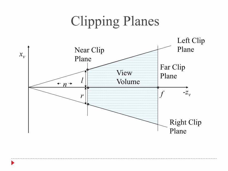
Clipping Planes
xv
-zv
Near Clip Plane
Far Clip Plane View
Volume
Left Clip Plane
Right Clip Plane
f n l
r
Where is the Image Plane?
} Notice that it doesn’t really matter where the image plane is located, once you define the view volume } You can move it forward and backward along the z axis and
still get the same image, only scaled
} The left/right/top/bottom planes are defined according to where they cut the near clip plane
} Or, define the left/right and top/bottom clip planes by the field of view
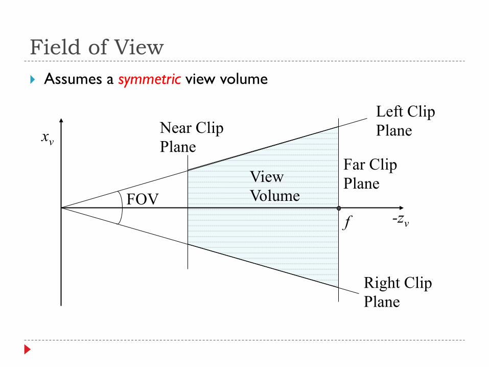
} Assumes a symmetric view volume
Field of View
xv
-zv
Near Clip Plane
Far Clip Plane View
Volume
Left Clip Plane
Right Clip Plane
f FOV
Perspective Parameters
} We have seen several different ways to describe a perspective camera } Focal distance, Field of View, Clipping planes
} The most general is clipping planes – they directly describe the region of space you are viewing
} For most graphics applications, field of view is the most convenient } It is image size invariant – having specified the field of view,
what you see does not depend on the image size
} You can convert one thing to another
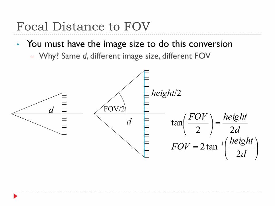
• You must have the image size to do this conversion – Why? Same d, different image size, different FOV
d d
FOV/2
height/2
⎟⎠
⎞⎜⎝
⎛=
=⎟⎠
⎞⎜⎝
⎛
−
dheightFOV
dheightFOV
2tan2
22tan
1
Focal Distance to FOV
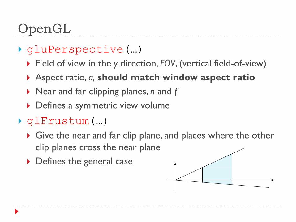
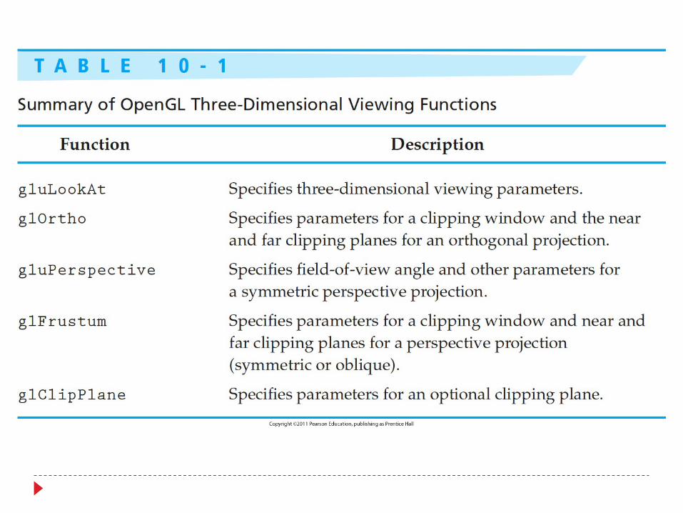
OpenGL
} gluPerspective(…) } Field of view in the y direction, FOV, (vertical field-of-view) } Aspect ratio, a, should match window aspect ratio } Near and far clipping planes, n and f } Defines a symmetric view volume
} glFrustum(…) } Give the near and far clip plane, and places where the other
clip planes cross the near plane } Defines the general case
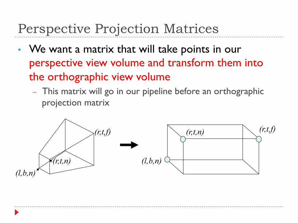
• We want a matrix that will take points in our perspective view volume and transform them into the orthographic view volume – This matrix will go in our pipeline before an orthographic
projection matrix
(l,b,n) (r,t,n) (l,b,n)
(r,t,n) (r,t,f) (r,t,f)
Perspective Projection Matrices
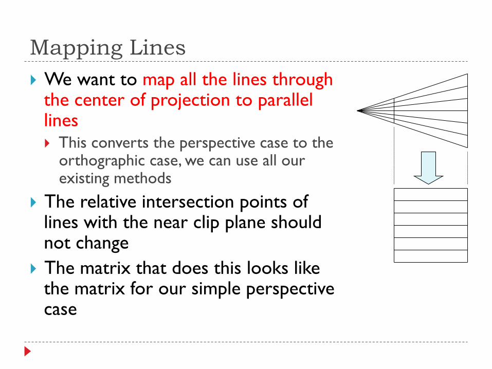
Mapping Lines } We want to map all the lines through
the center of projection to parallel lines } This converts the perspective case to the
orthographic case, we can use all our existing methods
} The relative intersection points of lines with the near clip plane should not change
} The matrix that does this looks like the matrix for our simple perspective case
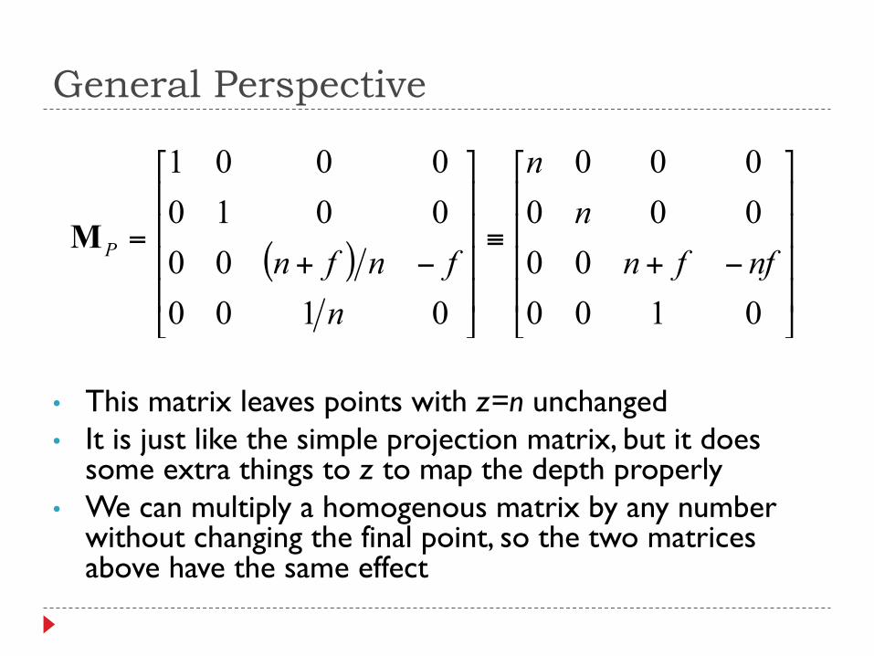
• This matrix leaves points with z=n unchanged • It is just like the simple projection matrix, but it does
some extra things to z to map the depth properly • We can multiply a homogenous matrix by any number
without changing the final point, so the two matrices above have the same effect
( )⎥⎥⎥⎥
⎦
⎤
⎢⎢⎢⎢
⎣
⎡
−+≡
⎥⎥⎥⎥
⎦
⎤
⎢⎢⎢⎢
⎣
⎡
−+=
010000
000000
010000
00100001
nffnn
n
nfnfnPM
General Perspective
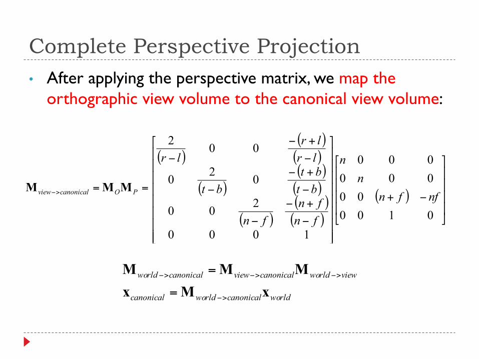
• After applying the perspective matrix, we map the orthographic view volume to the canonical view volume:
( )( )( )
( )( )( )
( )( )( )
( )⎥⎥⎥⎥
⎦
⎤
⎢⎢⎢⎢
⎣
⎡
−+
⎥⎥⎥⎥⎥⎥⎥⎥
⎦
⎤
⎢⎢⎢⎢⎢⎢⎢⎢
⎣
⎡
−
+−
−
−
+−
−
−
+−
−
==>−
010000
000000
1000
200
020
002
nffnn
n
fnfn
fn
btbt
bt
lrlr
lr
POcanonicalview MMM
worldcanonicalworldcanonical
viewworldcanonicalviewcanonicalworld
xMxMMM
>−
>−>−>−
=
=
Complete Perspective Projection
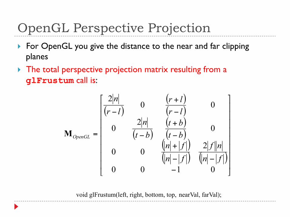
OpenGL Perspective Projection } For OpenGL you give the distance to the near and far clipping
planes } The total perspective projection matrix resulting from a glFrustum call is:
( )( )( )
( )( )( )( )( ) ( )
⎥⎥⎥⎥⎥⎥⎥⎥
⎦
⎤
⎢⎢⎢⎢⎢⎢⎢⎢
⎣
⎡
−−−
+−
+
−
−
+
−
=
0100
200
02
0
002
fnnf
fnfnbtbt
btn
lrlr
lrn
OpenGLM
void glFrustum(left, right, bottom, top, nearVal, farVal);
Near/Far and Depth Resolution } It may seem sensible to specify a very near clipping plane and a
very far clipping plane } Sure to contain entire scene
} But, a bad idea: } OpenGL only has a finite number of bits to store screen depth } Too large a range reduces resolution in depth - wrong thing may be
considered “in front” } See Shirley for a more complete explanation
} Always place the near plane as far from the viewer as possible, and the far plane as close as possible
} http://www.cs.rit.edu/~ncs/tinkerToys/tinkerToys.html
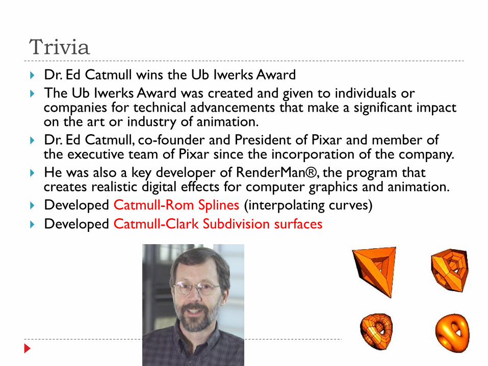
Trivia } Dr. Ed Catmull wins the Ub Iwerks Award } The Ub Iwerks Award was created and given to individuals or
companies for technical advancements that make a significant impact on the art or industry of animation.
} Dr. Ed Catmull, co-founder and President of Pixar and member of the executive team of Pixar since the incorporation of the company.
} He was also a key developer of RenderMan®, the program that creates realistic digital effects for computer graphics and animation.
} Developed Catmull-Rom Splines (interpolating curves) } Developed Catmull-Clark Subdivision surfaces