mohdruhaizie.commohdruhaizie.com/.../MohdRuhaizie_fyp_fullreport.docx · Web viewFINAL YEAR...
147
FINAL YEAR PROJECT PARTICULATE MATTER EXPOSURE COMPARISON IN INSPECTION BAYS AND OFFICES AT IMPORT LANE, SULTAN ABU BAKAR CIQ COMPLEX, JOHOR
Transcript of mohdruhaizie.commohdruhaizie.com/.../MohdRuhaizie_fyp_fullreport.docx · Web viewFINAL YEAR...
FINAL YEAR PROJECT
PARTICULATE MATTER EXPOSURE COMPARISON IN INSPECTION BAYS AND OFFICES AT IMPORT LANE, SULTAN ABU BAKAR CIQ
COMPLEX, JOHOR
MOHD RUHAIZIE BIN RIYADZI2010282848
HS 223
PARTICULATE MATTER EXPOSURE COMPARISON IN INSPECTION BAYS AND OFFICES AT IMPORT LANE, SULTAN ABU BAKAR CIQ
COMPLEX, JOHOR
MOHD RUHAIZIE BIN RIYADZI
Project paper submitted in partial fulfilment of the
requirements for the award of the Bachelor in
Environmental Health And Safety (Hons.)
Faculty of Health Sciences
JANUARY 2015
Declaration
This project paper entitled “PARTICULATE MATTER EXPOSURE COMPARISON IN INSPECTION BAYS AND OFFICES AT IMPORT LANE, SULTAN ABU BAKAR CIQ COMPLEX” is a presentation of my original work. Wherever contributions of others are involved, every effort is made to indicate this clearly, with due reference to the literature, and acknowledgement of collaborative research and discussions.
This work was done under the guidance of Mr. Megat Azman bin Megat Mokhtar (Project Supervisor) at the Mara University of Technology (UiTM).
(MOHD RUHAIZIE BIN RIYADZI)
In my capacity as supervisor of the candidate’s project, I certify that the above statements are true to the best of my knowledge.
(Megat Azman bin Megat Mokhtar)
Date :

Supervisor’s Signature
Project entitled “PARTICULATE MATTER EXPOSURE COMPARISON IN INSPECTION BAYS AND OFFICES AT IMPORT LANE, SULTAN ABU BAKAR CIQ COMPLEX” was prepared by Mohd Ruhaizie bin Riyadzi and has been submitted to the Faculty of Health Sciences in fulfilment of the requirement for the Bachelor In Environmental Health and Safety (Honours).
Accepted to evaluated by:
………………………………………….
(Megat Azman bin Megat Mokhtar)
Project Supervisor
Date : …………………………………..
ACKNOWLEDGEMENT
I would like to take this opportunity to express my sincere gratitude to all who have contributed in this study.
Alhamdulillahi rabbil alamin... first of all, I would like to deeply praise to Almighty Allah S.W.T. for His blessing and blissfulness for allowing me to complete this report in time and presentably.
It is millions of appreciation to mama Mdm. Ruhani binti Mohamad and abah Mr. Riyadzi bin Ahmad Shah for bringing such a joy in my life via your continuous Doa and positive encouragement.
In particular, I wish to express my sincere appreciation to my supervisor, Mr. Megat Azman bin Megat Mokhtar, for encouragement, support and guidance. I am also very thankful to all lecturers for their advice and recommendation on completing my final project.
Also a lot of thanks to Mr. Rumainor bin Sarif, the Deputy Director of State RMC Gelang Patah and the rest of RMC KSAB workforce especially those in Import Lane during the monitoring conducted for giving this opportunity to be in your daily working experience.
Thank you to Mr. Azali bin Bachok and the rest of Bahagian Pengurusan Hartanah, Jabatan Perdana Menteri (Bangunan Sultan Iskandar) for permit us to enter this restricted facility.

Thank you to the Director of DOSH Johor especially Mr. Kamaruzaman, Mr. Zulfikar and Mr. Redzuan from IH (IAQ) Unit, for not only lends me the equipments but also experiences and knowledge.
ACKNOWLEDGEMENT
Thank you to all friends in District Health Office of Johor Bahru, Port Health Office of Tanjung Pelepas Port, Port Health Office Puteri Harbor and Kompleks Sultan Abu Bakar Health Office especially Senior Assistant Environmental Health Officer Solihan Md. Ali.
Thank you to Team Epjj JB: Nur Adilah & Siti Aishah
Finally, my appreciation and special thanks also goes to my beloved family especially to my wonderful wife and the best friend of my entire life, SITI MASHALIDA BINTI JOHAR for the challenge we’ve faced together, for the support and for the love you give me until now.
My appreciation to Mr. Johar bin Kanchil and Mdm. Suhana binti Tukiran, my parent in-laws and the rest of my family for being very supportive through-out these 4 and half years journey.
I hereby inspire this work to all of my sons
Muhammad Amru Hakim, Ahmad Ariffin Billah & Muhammad Haziq Syafi
It’s a long journey, but no matter where it’s begin, the important is how it ends
15 years, 2 courses, 2 campuses and yet ends with one
Bachelor Degree in Environmental Health & Safety (Honours)

Thank you.
TABLE OF CONTENTS
DECLARATIONS
ACKNOWLEDGEMENT
LIST OF TABLES
LIST OF FIGURE
ABSTRACT
CHAPTER ONE : INTRODUCTION
INTRODUCTION 1
PROBLEM STATEMENT 4
STUDY JUSTIFICATION 5
STUDY OBJECTIVES 5
GENERAL OBJECTIVE 5
SPECIFIC OBJECTIVE 5
HYPOTHESIS 6
CONCEPTUAL FRAMEWORK 7

CONCEPTUAL DEFINITION 8
OPERATIONAL DEFINITION 9
CHAPTER TWO : LITERATURE REVIEW
PARTICULATE MATTER AND HEALTH PROBLEM 11
PARTICULATE MATTER AND RELATIONSHIP WITH VEHICLES 12
CLASSIFICATION OF PARTICULATE MATTER GROUPS 13
EXPOSURES TO PARTICULATE MATTER 14
INDOOR-OUTDOOR EXPOSURES OF PARTICULATE MATTER 15
PREVENTION AND CONTROL METHODS 16
CHAPTER THREE : METHODOLOGY
STUDY LOCATION 19
STUDY DESIGN 20
STUDY VARIABLES 20
INDEPENDENT VARIABLES 20
DEPENDENT VARIABLES 20
CONFOUNDING VARIABLES 21
SAMPLING AND DATA COLLECTION 21
INSTRUMENTATION 24
DATA ANALYSIS 25
STUDY LIMITATION 25
CHAPTER FOUR : RESULT
RESULT REGARDING SPECIFIC OBJECTIVE (1): TO MEASURE AIR
QUALITY PARAMETERS IN OUTDOOR AND INDOOR SETTINGS
26
PARTICULATE MATTER WITH DIAMETER SIZE OF 10 MICRONS
AND SMALLER (PM10)
26
PARTICULATE MATTER WITH DIAMETER SIZE OF 4 MICRONS
AND SMALLER (PM4)
31
PARTICULATE MATTER WITH DIAMETER SIZE OF 2.5 MICRONS
AND SMALLER (PM2.5)
33
PARTICULATE MATTER WITH DIAMETER SIZE OF 1 MICRONS
AND SMALLER (PM1)
35
TOTAL PARTICULATE MATTER (PMTOTAL) 37
TOTAL VOLATILE ORGANIC COMPOUND (TVOC) 39
CARBON DIOXIDE (CO2) 42
OZONE (O3) 44
CARBON MONOXIDE (CO) 47
AIR TEMPERATURE (AT) 49
RELATIVE HUMIDITY PERCENTAGE (%RH) 51
AIR VELOCITY 53
CONCLUSION FOR THE RESULT OF SPECIFIC OBJECTIVE (1) 54

RESULT REGARDING SPECIFIC OBJECTIVE (2): TO COMPARE THE
PARTICULATE MATTERS CONCENTRATION BETWEEN THE
OUTDOOR AND INDOOR SETTINGS
56
CONCLUSION FOR THE RESULT OF SPECIFIC OBJECTIVE (2) 59
RESULT REGARDING SPECIFIC OBJECTIVE (3): TO IDENTITY THE
RELATIONSHIP BETWEEN PARTICULATE MATTER AND OTHER
PARAMETERS IN THE OUTDOOR AND IN THE INDOOR SETTINGS
61
RESULT REGARDING SPECIFIC OBJECTIVE (4): TO CALCULATE
PARTICULATE MATTER INDOOR-OUTDOOR (I/O) RATIO
63
CHAPTER FIVE: DISCUSSION 68
INDOOR-OUTDOOR (I/O) RATIO 72
COMPARING DATA WITH LEGAL REQUIREMENTS AND STANDARDS 73
CHAPTER SIX: RECOMMENDATION AND CONCLUSION 76
REGARDING THE VEHICLE 76
REGARDING THE BUILDING 77
REGARDING THE PEOPLE 79
CONCLUSION 80
REFERENCES 81

APPENDICES 86
LIST OF TABLES
Table 3-1 Sampling location in Import Lane, KSAB
Table 3-2 Sampling location sequence within three days of study conducted in
Import Lane, KSAB
Table 4-1 Results for each day TWA8hrs and TWA24hrs calculation from the PM10
concentration data obtained in Figure 4-1, and comparison with ICOP
IAQ 2010 and MAAQG, respectively.
Table 4-2 Results for each day TWA8hrs calculation from the TVOC
concentration data obtained in Figure 4-11, and comparison with
ICOP IAQ 2010
Table 4-3 Results for each day TWA8hrs calculation from the CO2 concentration
data obtained in Figure 4-13, and comparison with ICOP IAQ 2010
Table 4-4 Results for each day TWA8hrs calculation from the ozone
concentration data obtained in Figure 4-15, and comparison with
ICOP IAQ 2010 and MAAQG, respectively.
Table 4-5 Results for each day TWA8hrs calculation from the CO concentration
data obtained in Figure 4-17, and comparison with ICOP IAQ 2010
and MAAQG, respectively.
Table 4-6 Output results for descriptive statistics after analysis of Kruskal-Wallis
Non-Parametric Test (K-Independent Sample) has been run in SPSS.
Table 4-7 Output results for the Mean Rank
Table 4-8 Output results for the Test Statistics (Chi-Square, X2)
Table 4-9 Output results for the Frequency
Table 4-10 Output results for the Test Statistics (median)
Table 4-11 Spearman’s correlation output results. The table is been simplified to
fit the page
Table 4-12 Descriptive statistics output when the concentration of particulate
matter is separated in specific location settings with N=13 for each
setting

LIST OF FIGURES
Figure 1-1 Air Pollution Index used by Department of Environment Malaysia
Figure 1-2 Air Pollution Index in Johor in year 2013
Figure 1-3 Print-screen from GoogleMaps of a satellite view showing the location
of KSAB. Note: the light-orange lines is SecondLink Highway which
connecting Malaysia (to the left, upward) and Singapore (to the right,
downward).
Figure 1-4 Conceptual Framework
Figure 3-1 Print-screen from GoogleMaps of a satellite view showing the location
of KSAB (marked with the red downward arrow)
Figure 3-2 Import Lane of KSAB, consist inspection bay and offices
Figure 4-1 30-minutes averages PM10 concentration at different location within 3
days of study (upper horizontal redline: acceptable upper limit: 0.15
mg/m3, TWA8hrs (ICOP IAQ 2010, DOSH); 150 µg/m3, TWA24hrs
(MAAQG, DOE))
Figure 4-2 (Left) Histogram of the data distribution and normality curve; (Right)
Descriptive statistics table for PM10
Figure 4-3 30-minutes averaged PM4 concentration at different location within 3
days of study

Figure 4-4 (Left) Histogram of the data distribution and normality curve; (Right)
Descriptive statistics table for PM4
Figure 4-5 30-minutes averaged PM2.5 concentration at different location within 3
days of study
Figure 4-6 (Left) Histogram of the data distribution and normality curve; (Right)
Descriptive statistics table for PM2.5
Figure 4-7 30-minutes averaged PM1 concentration at different location within 3
days of study
Figure 4-8 (Left) Histogram of the data distribution and normality curve; (Right)
Descriptive statistics table for PM1
Figure 4-9 30-minutes averaged PMTOTAL concentration at different location within
3 days of study
Figure 4-10 (Left) Histogram of the data distribution and normality curve; (Right)
Descriptive statistics table for PMTOTAL
Figure 4-11 30-minutes averaged TVOC concentration at different location within
3 days of study (the horizontal redline: acceptable upper limit: 3 ppm,
TWA8hrs (ICOP IAQ 2010, DOSH))
Figure 4-12 (Left) Histogram of the data distribution and normality curve; (Right)
Descriptive statistics table for TVOC
Figure 4-13 30-minutes averaged CO2 concentration at different location within 3
days of study (the horizontal redline: acceptable upper limit: C1000
ppm, TWA8hrs (ICOP IAQ 2010, DOSH))
Figure 4-14 (Left) Histogram of the data distribution and normality curve; (Right)
Descriptive statistics table for carbon dioxide
Figure 4-15 30-minutes averaged ozone concentration at different location within
3 days of study (upper horizontal redline: acceptable upper limit: 0.05
ppm, TWA8hrs (ICOP IAQ 2010, DOSH); 0.06 ppm, TWA8hrs (MAAQG,
DOE))
Figure 4-16 Figure 4-16 (Left) Histogram of the data distribution and normality
curve; (Right) Descriptive statistics table for ozone
Figure 4-17 30-minutes averaged carbon monoxide concentration at different
location within 3 days of study (the horizontal redline: acceptable
upper limit: 10.0 ppm, TWA8hrs (ICOP IAQ 2010, DOSH); the
horizontal purple line 9.0 ppm, TWA8hrs (MAAQG, DOE))
Figure 4-18 (Left) Histogram of the data distribution and normality curve; (Right)
Descriptive statistics table for carbon monoxide
Figure 4-19 30-minutes averaged air temperature at different location within 3
days of study (the horizontal redline: acceptable range: 23.0 ⁰C –
26.0 ⁰C, (ICOP IAQ 2010, DOSH))
Figure 4-20 (Left) Histogram of the data distribution and normality curve; (Right)
Descriptive statistics table for air temperature
Figure 4-21 30-minutes averaged relative humidity percentage at different location
within 3 days of study (the horizontal redline: acceptable range: 40 %
– 70 % (ICOP IAQ 2010, DOSH))
Figure 4-22 (Left) Histogram of the %RH data distribution and normality curve;
(Right) Descriptive statistics table for %RH
Figure 4-23 30-minutes averaged air velocity at different location within 3 days of
study (the horizontal redline: acceptable range: 0.15 m/s – 0.50 m/s
(ICOP IAQ 2010, DOSH))
Figure 4-24 (Left) Histogram of the air velocity data distribution and normality
curve; (Right) Descriptive statistics table for air velocity

ABSTRACT
In Sultan Abu Bakar CIQ Complex (KSAB), Johor, Royal Malaysia Customs (RMC)
and other government agencies (OGA) officers are placed in offices building next to
the inspection bays in either Import Lane or Export Lane. They’re facing hustle bustle
traffic of heavy-duty carriers (HDC), which most of them using diesel as fuel,
everyday. HDC especially the one using diesel is commonly known as the major
contributor to the particulate matter pollutions globally. A study has been conducted
in 3 days in Import Lane, involving 26 sampling locations (13 outdoors, 13 indoors),
generally to compare the concentration of PM indoor and outdoor, using TSI®
DustTrakTM DRX handheld device. For other air quality parameters, HP iPAQ 2010
Pocket PC is used to log data which is monitored using GrayWolf® DirectSense® IQ-
610 Indoor Air Quality Probe and AS-210 Telescoping Hotwire Probe. Each
measurement is done in 30-minutes with data logged every 2 minutes. Data obtained
is analysed using Mircosoft Excel 2010 for graph manipulation and IBM SPSS 16.0
statistic analysis. During peak hour, the concentration of PM (all type) is increased.
There is no statistically significant difference between concentration of PM indoor and
outdoor (p > 0.005), where the I/O ratio is ranged between 0.748 (PM10) and 0.795
(PM1), where as diameter of particles getting smaller, the I/O ratio become higher. In
this study, Spearman’s Correlation Test found that air temperature has significant
relationship with PM with strong, positive correlation (p < 0.001). For mitigation
measures, it is suggested administrative approaches is used against the HDC itself,
and combination of strategies as stipulated by Maroni (1998) against the buildings
environment. Air curtain is suggested to be used as air shield to hold pollutants in the
outdoor entering indoor environment.
Keyword: particulate matter, indoor settings, offices, outdoor environment, inspection
bay, heavy-duty carriers, entry-point enforcement workforce
ABSTRAK
Di Kompleks KIK Sultan Abu Bakar (KSAB), Johor, pegawai-pegawai Jabatan
Kastam Diraja Malaysia dan lain-lain agensi kerajaan (OGA) ditempatkan di
bangunan pejabat bersebelahan dengan ruang pemeriksaan, sama ada di laluan
import ataupun laluan eksport. Mereka berhadapan dengan kesibukan trafik
kenderaan-kenderaan berat yang kebanyakkannya menggunakan diesel sebagai
bahan bakar, yang diketahui menyebabkan pencemaran partikel secara global.
Kajian dijalankan selama 3 hari di laluan import, melibatkan 26 lokasi persampelan
(13 lokasi luaran, 13 lokasi dalaman), secara umumnya untuk membandingkan
konsentrasi partikel dalam udara luaran dan dalaman, menggunakan TSI®
DustTrakTM DRX, manakala untuk lain-lain parameter menggunakan HP iPAQ 2010
Pocket PC yang melog data dari GrayWolf® DirectSense® IQ-610 Indoor Air Quality
Probe dan AS-210 Telescoping Hotwire Probe. Setiap pengukuran dilakukan dalam
tempoh 30-minit dengan data dilog setiap 2 minit. Data yang diperolehi dianalisa
menggunakan Mircosoft Excel 2010 untuk manipulasi graf dan IBM SPSS 16.0 untuk
analisa statistik. Ketika waktu puncak, konsentrasi partikel (semua jenis) adalah
meningkat. Tiada perbezaan statistic yang signifikan dikenas antara konsentrasi
partikel dalam udara luaran dan dalaman (p > 0.005), dengan nisbah I/O di antara
0.748 (PM10) dan 0.795 (PM1), di mana semakin kecil saiz diameter partikel, nisbah
I/O semakin meningkat. Dalam kajian ini, Spearman’s Correlation Test menunjukkan
suhu udara mempunyai korelasi signifikan yang kuat dan positif dengan PM (p <
0.001). Sebagai langkah mengatasi masalah, dicadangkan pendekatan
administrative digunakan ke atas isu kenderaan berat dan kombinasi strategi
sebagaimana yang dicadangkan oleh Maroni (1998) untuk mengatasi masalah
berkaitan bangunan. “Air curtain” adalah dicadangkan untuk digunakan sebagai
perisai udara untuk menghalang kemasukan bahan cemar dari luar ke persekitaran
dalaman.
Keyword: particulate matter, indoor settings, offices, outdoor environment, inspection
bay, heavy-duty carriers, entry-point enforcement workforce

CHAPTER ONE
INTRODUCTION
Clean and fresh air to breathe has been concern since several decades ago. It’s even
a requirement as stipulate in the ancient yoga proverb “for breathe is life, and those
who breathe well, live longer”. Although this proverb is meant for the better breathing
techniques, it will be useless when someone breathe well, but breathe in unclean air.
Air is one of the medium used by pollutants and pathogens to enter human body
through route of entry known as inhalation. According to World Health Organization,
one of the environmental health risks is air pollution which is related to the
emergence of respiratory problem such as acute respiratory diseases including
asthma, allergy and irritation, strokes, lung cancer etc.
According to Ministry of Health Malaysia (2013), among ten principal causes of
hospitalization in Ministry of Health Hospital and private hospital in 2012, disease of
the respiratory system is ranked as second (12.08%). Disease of the respiratory
system is also ranked at the same spot among ten principal causes of death in
Ministry of Health Hospital and private hospital in 2012 (17.90%). Diseases of
respiratory problems are including lung cancer, breathing problem, sore throat and
irritating, influenza, tuberculosis etc. Most of the chronic disease related to the
respiratory are mostly due to breathing the unhealthy air (air pollution) as well as
unhealthy lifestyle including smoking.
Air pollution index (API) is set by Department of Environment Malaysia as the
indicator to evaluate how cleaness the ambient air everyday. The components that
formed the API are carbon monoxide (CO), ozone (O3), nitrogen dioxide (NO2) and
sulfur dioxide (SO2) and particulate matter (PM10). The indication of API is as follows:

API Air Pollution Level
0 - 50 Good
51 - 100 Moderate
101 - 200 Unhealthy
201 - 300 Very unhealthy
301 - 500 Hazardous
500+ Emergency
Figure 1-1 Air Pollution Index used by Department of Environment Malaysia
In Johor, there are four sampling stations to measure daily the volume of pollutant in
the air. These stations are located in Kota Tinggi, Larkin Lama (Johor Bahru), Muar
and Pasir Gudang (Johor Bahru). The API for Johor in year 2013 is as in Figure 1-2
above. In Larkin Lama which is closed to the centre and western region of Johor
Bahru, API for 300 days appears to be in “Good” conditions (API 0 – 50), while the
other 65 days, the API is “Unhealthy” (API 101 – 200).
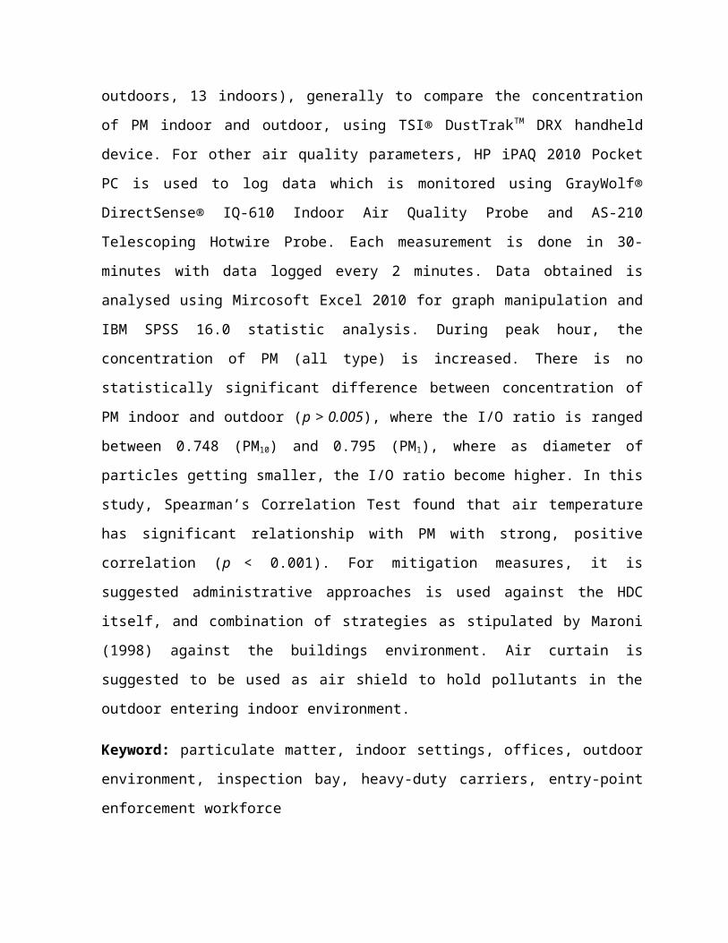
Figure 1-2 Air Pollution Index in Johor in year 2013
One of the government facility located in western region of the Johor Bahru is Sultan
Abu Bakar Custom, Imigration & Quarantine (CIQ) Complex (abbreviate: KSAB)
(GPS: 1.377738, 103.599140). It’s a ground crossing checkpoint facility that play role
in controlling travellers and conveyances at the country border which connecting
Malaysia and Singapore through a highway route known as SecondLink (E3), which
is also managed by PLUS Berhad, instead of PLUS Highway (E2) itself.
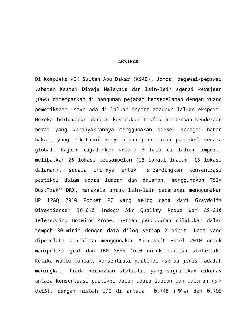
Figure 1-3 Print-screen from GoogleMaps of a satellite view showing the location
of KSAB. Note: the light-orange lines is SecondLink Highway which
connecting Malaysia (to the left, upward) and Singapore (to the right,
downward).
According to the Properties Management Division, Prime Minister Department of
Malaysia, this border control facility is designed to accept a maximum of 200,000
vehicles daily, which 25% to 35% of the vehicles are estimated as heavy duty
carriers. The number of heavy duty carriers may reachs up to 40% of the total
number of vehicles in Friday, as it is the last weekday for official business hour in
Singapore.
All heavy duty carriers must be inspected for goods or consignments they’re carrying
either for importation to Malaysia purpose or exportation to Singapore purpose. The
inspection process including declaration of the goods carried, physical and sampling
examination by Royal Malaysia Customs (RMC) or other government agencies
(OGA), sealing of the conveyance cover and consignment released.
Problem Statement
Several RMC and OGA (such as Department of Health, Department of
Pharmaceutical Enforcement, Malaysian Quarantine and Inspection Services
(MAQIS) (a governmental body formed by combination of departments under Ministry
of Agriculture and Agro-Based Industry (MOA)) and Department of Wildlife Protection
etc.) offices is placed near to the inspection bays either in Import Lane or Export Lane
in KSAB. This is to ease the forwarding agents, importer or exporter representative as
well as officers from both RMC and OGA in declaring the consigment, conducting
examination and approving either exportation or importation.
As the offices is placed near the inspection bays, occupants inside may be exposed
themselves to the unclean and unhealthy air as well as noise which penetrated from
the outside. The exposure may be greater especially when they’re out to the
inspection bay. This unclean and unhealthy air may penetrate to the indoor settings
of these office thus affected the indoor air quality.
According to Brugge (2007), heavy weight carriers such as trucks are potentially
emitted higher concentration of pollutants compared to the light weight vehicles such
as cars, thus make it significant source of urban air contamination now days. As
nearer as someone to the source of contamination, the higher volume of exposure
will she or he get
This condition, sooner or later, may affecting the health of the exposed person
(Moller, 2014).
Study Justification
Department of Health in KSAB has undergone an assessment and evaluation by the
representative of International Health Sector, Disease Control Division, Ministry of
Health Malaysia in year 2012 in fulfilling the requirement of establishing core
capacities as stipulated in Annex 1 B of International Health Regulations (IHR) 2005.
One of the requirement is to ensure the travellers as well as workforce in entry point
is in clean and healthy environment, both in outdoor and indoor settings.
However, until today, the Indoor Air Quality Assessment haven’t been done, thus
there is no clue how does the working environment status in KSAB for both outdoor
and indoor settings.
Therefore, this study may help the governmental agencies including to understand
the level of exposure of air quality parameters especially particulate matter
concentrations faced by the officers, staffs and other people who have business
matter regarding with importation and exportation of consignments.
Study Objectives
(1) General Objective
To compare the exposures of particulate matter in the outdoor (inspection
bays) and in the indoor settings (offices) at Import Lane, Sultan Abu Bakar
CIQ Complex.
(2) Specific Objectives

a. To measure air quality parameters in outdoor and indoor settings
(PM10, PM4, PM2.5, PM1, PMTOTAL, TVOC, CO2, O3, CO, relative
humidity, air temperature and air velocity)
b. To compare particulate matter concentrations between the outdoor
and the indoor settings
c. To identify the relationship between particulate matter and other
parameters in the outdoor and in the indoor settings
d. To calculate the particulate matter indoor-outdoor (I/O) ratio
Study Hypothesis
(1) For specific objective (2) above, there will be no statistical significant
difference between particulate matter concentration in the outdoor and in
the indoor settings
(2) For specific objective (3) above, concentration of particulate matter may be
influenced with other air quality parameters in both outdoor and indoor
settings; and
(3) For specific objective (4) above, for overall, the concentration of particulate
matter in the outdoor may be greater than the particulate matter
concentration indoor.
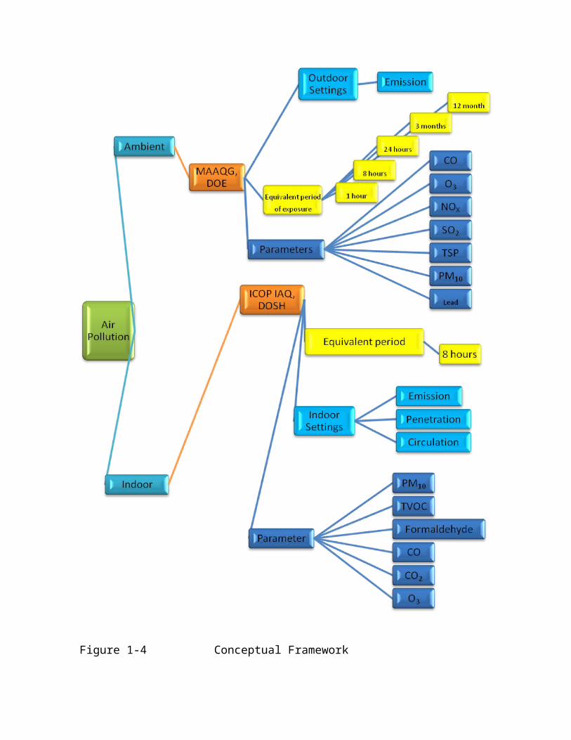
Conceptual Framework

Figure 1-4 Conceptual Framework
Conceptual Defination

(1) Air pollution
As air is around everywhere and everytime, it is the most suitable medium
for pathogens and pollutants to caused adverse effect either on the health of
human, animal or even crops, but also built environment. In KSAB, officers
and other people works or have business matter within it compound as well
as travellers faced the exposure of variety of air pollutants either in the
indoor setting or the outdoor environment.
(2) Souce of air pollution
Commonly known, source of pollution can be either natural or
anthropogenic. In every of the sources, it can be categorised into two:
stationary source of mobile source. In KSAB, the major air pollution source
is due to the vehicles which crossed the terminal, where it is estimated
about this entry point facility can hold for about 200,000 maximum number
of vehicles daily. 25 – 35% or even 40% of these number of vehicles is
heavy duty carrier or heavy weight vehicles which play on important role in
import export industries across the land.
(3) Regulatory standards
For the ambient air pollution, the concentration of pollutants is measured
and then compared with Malaysia Ambient Air Quality Guidelines published
b y Department of Environment Malaysia. The parameters are ozone,
carbon monoxide, nitrogen oxides, sulfur dioxide, total suspended particles,
particulater matter (PM10) and lead, with the measurement period should be,
or equivalent to, ranged from 1 hour to 12 months. For indoor air quality, the
concentration of pollutants is measured and then compared with Malaysia
Ambient Air Quality Guidelines published b y Department of Environment

Malaysia. The parameters are ozone, carbon monoxide, carbon dioxide,
particulater matter (PM10) formaldehyde, total volatile organic compounds,
microbological contaminants (bacteria and fungi) and several physical
parameters (air velocity, air temperature and relative humidity), with the
measurement period should be, or equivalent to 8 hours.
Operational defination
(1) Heavy duty carrier or heavy weight vehicle
A vehicle used to carry importation or exportation purposed consignment
across the terminal either to Singapore or to Malaysia. The vehicle is
permitted to only driven through the designated lane (Importat Lane or
Exported Lane) and must not carry human. Every vehicle that enter the
inspection bay either just to crossed it to the exit route or parked in it or
surround it while the declaration of consignment have been made until
importation or exportation is permitted is count as 1, regardless the period
the vehicle stay in the inspection bay or surround it, either the engine in idle
mode or switched off.
(2) Measurement of outdoor environment
The measurement of outdoor environment must only be made under the
roof of the inspection bay although the facility is open to the ambient air (no
walls), but not to closed to the pillar and regardless to any vehicle parked
nearby. Measurement must be made in-situ where the average data is
obtained once the period of measurement is done per each location.

(3) Measurement of indoor settings
The measurement of outdoor environment must only be made inside the
office which is opposite right to the sampling location chosen and used for
the outdoor environment monitoring. The measurement must be made
starting within the interval 5 minutes after the end of each outdoor
environment. At each indoor location, instrument must be made in the
centre of the given space. Measurement must be made in-situ where the
average data is obtained once the period of measurement is done per each
location.

CHAPTER TWO
LITERATURE REVIEW
Particulate matter and health problem
In many literatures reviewed, particulate matter has been a focus and concern among
health environmentalists and occupational safety & health practitioners since
decades regarding air pollution issue.
According to World Health Organization and United States Environmental Protection
Agency, among six major air pollutants, particulate matter with diameter size of 10
micrometers or lesser has potentially harming human health with the association in
lung cancer, respiratory tract problem/disease, cardiovascular disease, asthma, and
premature death which is linked to the air pollution. The latest study by Moller et al
(2014) linked the latest concern among particulate matters, the ultrafine particulate
matter (particulate diameter size is less than 100nm or 0.1 microns, abbreviated as
UFP) with cardiovascular disease and lung cancer. According to Janssen et al
(2001), children who attending school near the motorway sometimes has been
brought to pay a visit in the emergency section in health care facilities/hospital due to
the exposure of fine particulate matter (diameter size 2.5 microns or less).
Among six WHO Regional Office worldwide, Western Pacific Regional Office (WPRO)
and South East Asia Regional Office (SEARO) faces the greatest challenges as
health impact due to air pollutants exposure become the greatest burden in the most
low and middle income countries in under both WHO entities supervision. Malaysia
and Singapore are among State Parties in WPRO.
Particulate matter and relationship with vehicle
As more study has been conducted, it is clear that transportation industry is the main,
important and significant sources for particulate matter pollution globally. According to
Weijers et al (2004), the increasing degree of urbanization which one of the indicators
is the increasing degree of development and number of industries as well as
transportation services and degree of traffic condition have a strong, positive
correlation with particulate matter pollution now days.
Among varieties of vehicle type, heavy duty carriers, also termed as heavy weight
vehicles or heavy diesel driven vehicle due most of this vehicle type fuelled by diesel
for power to move, are identified to be the major contributor to particulate matter,
nitrogen oxides and sulphur dioxide as well as carbon monoxide and tropospheric
ozone emission to the outdoor environment (Clark et al, 1999; Naeher et al, 2000;
Colvile et al, 2001; Charron et al, 2005; Brugge et al, 2007; Sheesley et al, 2008; &
Garshick et al, 2012).

Classification of particulate matter groups
U.S. EPA was firstly determined particulates which the size of 10 microns and smaller
as inhalable particles. Then, several researches determine that there variety of
particles size. According to Estokova and Stevulova (2012), particulate matter is
classified into several groups as accordance to their diameter size (particle size
distribution).
Inhalable particle is particulate matter with the diameter size of 10 and lesser. The
symbol used for this group of particle is PM10. It is also known as aerosol particulate.
This small size is an advantage to the particles to deposit in the deepest part of the
lungs (bronchioles and alveoli) (U.S. EPA). Another group is respirable particle, with
diameter of 4 microns or smaller, abbreviated with the symbol PM4.
Coarse particle is an identification of a group of particulate matter which have
diameter size larger than fine particles but smaller than inhalable particles (range
from > 2.5 μm to ≤ 10.0 μm) (Estokova and Stevulova, 2012).
Particle with diameter size of 2.5 and lesser is known as fine particulate, symbolised
with PM2.5. It can penetrate deeper up to alveolus, the gas exchange region in the
lung thus disturbing the process. According to Grau-Bove and Strlic (2013), PM2.5 is a
good indicator of the amount of anthropogenic particulate pollutants in urban ambient.
It has significant correlation with nitrogen oxides in emitted from vehicular exhaust
(Gillies et al, 2001). Another type of particle which is categorised as fine particles is
PM1 (diameter size of 1 micron or less), which is mostly originated from combustion
process and have high content of inorganic carbon compound.
Today, the smallest fraction of particulate matter is known as ultrafine particles (UFP).
It has a diameter size of 0.1 microns (100 nanometre) or less. The characteristic of
UFP such as high alveolar deposition fraction, insolubility, large surface area and
toxic constituents has ability to pass through cell membranes into the blood vessel,
migrate into other vital organ including the brain. UFP can carry carcinogens by
absorbing in it surface then deposit it at the destination organ (Moller, 2014).
Exposures to particulate matter
Higher concentration of particulate matter can be found as emission of vehicular
exhaust (higher in diesel driven heavy weight vehicle compared to the light weight
vehicle), as well as emission from industries, during traffic congestion and as a result
from re-suspension of roadside dust (Wahlina et al, 2001; Gillies et al, 2001; Marr et
al, 2004; Charron et al, 2005; Jones & Harrison, 2006; Brugge et al, 2007; Kaur et al,
2007; Sheesly et al, 2008; Thorpe & Harrison, 2008; Yu-Hsiang et al, 2012).
According to Weijers et al (2004), air movement and direction have significant
relationship with particulate matter exposure. People who live or at the downwind
level from the roadside (including highway) have exposed to more than 40% higher in
particulate matter concentration compared to those who lives in the busy urban
environment.
Indoor-outdoor exposure of particulate matter
According to WHO, indoor air quality is associates with the quality of the ambient air.
According to Lawrence et al (2004), the level of carbon monoxide concentration in
indoor settings has positive correlation with the outdoor concentration of carbon
monoxide. He suggests that there are no statistical significant differences between
both settings. Meanwhile, there is strong, positive correlation between particulate
matter and carbon monoxide (Kaur et al, 2007). Therefore, it is obvious that the
pollutants from outdoor may contaminate the indoor condition.
According to Chun & Bin (2011), pollutants from the outdoor enter the indoor
environment through several ways including direct entrance through any opening, or
through penetration in the wall cracks or leaks of infiltration through smaller gap
between joint and fixture of wall, ceiling etc. There are three parameters to determine
the relationship between indoor and outdoor concentration of particles: (1) I/O ratio;
(2) infiltration factor; and (3) penetration factor.
According to Grau-Bove & Strlic (2013), I/O ratio is widely used to describe the
condition between both settings. In their study they found that, due the aerodynamic
properties of the particulate matter based on their size, particulate matter with smaller
size will have higher I/O ratio. This also can be concluded that, when coming from the
same source, concentration of particulate matter with smaller diameter size are
higher in indoor setting compared to the larger diameter sized of particulate matter.
Prevention and control methods
Maroni (1998) suggest two main strategies which needs to be combined to achieved
indoor air quality control and improvement: (1) the built structure (the building itself)
needs to be designed and constructed properly; and (2) indoor air pollutants must be
controlled using one or combination of methods either control the source, having
adequate ventilation, cleaning the air or control the exposure group.
According to Kaur et al (2007), the best way to prevent and control the exposure of
air pollution is by avoiding the source that emitted it, such as avoid from being nearer
the construction area. However this seems impossible to be done in the area where
heavy vehicle is compulsory.
According to Bailey & Solomon (2004), in the seaport environment where not only
vessel emit the air pollutants but also the ground vehicle such as prime mover (PM)
or rubber tyre gantry (RTG), the mitigation measure should account wide range of
possibilities from the existing and cheaper to the investment and costly-required
control measures. They take an example of restricting all prime mover drivers from

idling or to switch off the haulier engine while stopping at designated parking area or
while waiting the order and to use low sulphur content of the diesel.
Wiejers et al (2014) suggest an air bending device to be install. As pollutants
movement is based on the wind direction and velocity, air bending device will divert
the pathway of the pollutant. Example of air bending device is suction pipe which is
suggested to be installed on the road surface where the lower pressure inside the
suction pipe will attract wind direction to it thus it can channel the pollutant to the area
where it exposure may not be significantly adverse to other around. More example of
air bending device is air curtain. Air curtain is mostly used in vector control program.
However the same principle may be applied in air quality control, where the higher
velocity of the air flown down shielding any opening from being penetrated or
infiltrated by lower air velocity from the proportioned direction.
More than that, in a regularly closed room where the number of door and window
opening activity is seldom occurred, the room may be sure to have a positive
pressure inside by promoting good ventilation and higher frequency of air change.
According to WHO, several preventive and control measures can be applied in air
quality control as follow:
1) Licensing source of emission. Before the license could be granted, the emitter
needs to be evaluated for the compliances toward cleaner air standard.
Emitter may not only require installing devices such as catalytic converter to
reduce carbon monoxide emission in exhaust system, but to ensure the
regular maintenance and self-monitoring. Based polluter pay policy and on the
data gathered through licensing activity, emitter may require paying tax on fuel
and carbon.
2) Where the place is suitable, the restriction of smoking in designated non-
smoking area need to be regulated as a law requirement and enforced to
uphold it.
3) The policy for regularly monitoring and control the indoor air quality standard
need to be applied as soon as possible. Currently, several country has already
regulate their own set of guideline regarding indoor air quality as to ensure
good practices regarding occupational safety, health and hygiene, but it is just
as a role of guideline. Once regulated as legislative document, it can be
enforced for better air to breathe in indoor setting.
4) Shifting to cleaner heavy duty vehicles and low-emission vehicle and fuels,
reduced sulphur content in the fuel.
5) More than that, a regulation needs to be setting up to require all vehicles,
especially heavy duty vehicle to turn off the engine once stop at any
designated parking.

CHAPTER THREE
METHODOLOGY
Study Location
KSAB is located in Bukit Kucing, Mukim Tanjung Kupang, at the western region of
Johor Bahru District, which is about 15 kilometres from Gelang Patah Town; 25
kilometres from Johor State New Administrative Centre (JSNAC) in Kota Iskandar,
Nusajaya; 40 kilometres from the centre of Johor Bahru metropolitan; and 50
kilometres from the Senai Airport. The GPS coordinate is 1.378066, 103.599218.
Figure 3-1 Print-screen from GoogleMaps of a satellite view showing the location
of KSAB (marked with the red downward arrow)
This complex can be accessed via the inner route of Jalan Tanjung Kupang – Gelang
Patah or via SecondLink Highway (E3). However, as this complex is restricted area,
the entrance connected with the inner route can only be accessed by authorised
personnel.

Historically, this complex and SecondLink Highway was officially opened in January
2, 1998 to ease the traffic problems between Malaysia and Singapore at Tanjung
Puteri CIQ Complex (Johor Causeway). It’s a new link between Malaysia (at
Kampung Tanjung Kupang) and Singapore (at Tuas). The opening ceremony was
officiated by Prime Minister of Malaysia at that time, Datuk Seri Dr. Mahathir
Mohamad (now Tun).
Study Design
This is a cross-sectional study in which the data is collected from several samples at
one point in time and then by comparing the difference between characteristic found
in all samples, a conclusion is made of (Leslie G.P. and Mary P.W., 2009).
Study Variables
(1) Independent Variable
a. Location of the sampling point either in the outdoor environment or in
the indoor settings
b. Days either it is on Singapore’s weekdays (working days) and
weekends (non-working days).
(2) Dependent Variable
a. In-situ parameters of ambient air quality and indoor air quality:
i. Particulate matters (PM10, PM4, PM2.5, PM1 & PMTOTAL)
ii. Carbon dioxide (CO2)
iii. Carbon monoxide (CO)
iv. Ozone (O3)
v. Total volatile organic compound (TVOC)
vi. Air temperature
vii. Air velocity

viii. Relative humidity
(3) Confounding Variable
a. Number of vehicle, other than heavy weight vehicle, used by the officers
and agents, crossing the study location.
b. Number of people and their activities near the measurement instrument
c. The condition of mechanical ventilation air conditioning (MVAC) system,
either cleaned or not, functioning or switches off etc.
d. The environmental influences such as weather, ambient dust etc.
Sampling and data collection
(1) There are 10 sampling locations which were visited during this study, which 5
are in the outdoor environment (inspection bays) and another five in the
indoor-settings (offices).
(2) All probes are set to be at the same height as breathing area in sitting
position (approximately 1 metre height from the floor level).
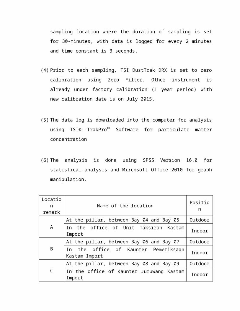
(3) Each sampling is done for average 30-minutes (grab sampling techniques,
ICOP IAQ 2010 - Methodology) at each sampling location where the duration
of sampling is set for 30-minutes, with data is logged for every 2 minutes and
time constant is 3 seconds.
(4) Prior to each sampling, TSI DustTrak DRX is set to zero calibration using
Zero Filter. Other instrument is already under factory calibration (1 year
period) with new calibration date is on July 2015.
(5) The data log is downloaded into the computer for analysis using TSI®
TrakProTM Software for particulate matter concentration

(6) The analysis is done using SPSS Version 16.0 for statistical analysis and
Mircosoft Office 2010 for graph manipulation.
Location remark Name of the location Position
AAt the pillar, between Bay 04 and Bay 05 OutdoorIn the office of Unit Taksiran Kastam Import Indoor
BAt the pillar, between Bay 06 and Bay 07 OutdoorIn the office of Kaunter Pemeriksaan Kastam Import Indoor
CAt the pillar, between Bay 08 and Bay 09 OutdoorIn the office of Kaunter Juruwang Kastam Import Indoor
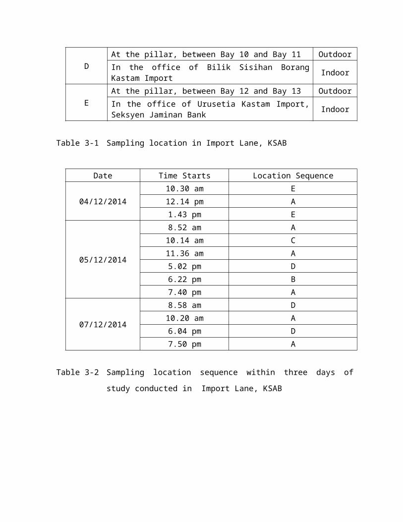
DAt the pillar, between Bay 10 and Bay 11 OutdoorIn the office of Bilik Sisihan Borang Kastam Import Indoor
EAt the pillar, between Bay 12 and Bay 13 OutdoorIn the office of Urusetia Kastam Import, Seksyen Jaminan Bank Indoor
Table 3-1 Sampling location in Import Lane, KSAB
Date Time Starts Location Sequence
04/12/201410.30 am E12.14 pm A1.43 pm E
05/12/2014
8.52 am A10.14 am C11.36 am A5.02 pm D6.22 pm B7.40 pm A
07/12/2014
8.58 am D10.20 am A6.04 pm D7.50 pm A
Table 3-2 Sampling location sequence within three days of study conducted in
Import Lane, KSAB
Figure 3-2 Import Lane of KSAB, consist inspection bay and offices
EDCB
A
A
Instrumentation
(1) TSI® DustTrakTM DRX model 8534 (handheld) with Zero Filter
(2) HP iPAQ 210 Pocket PC
(3) GrayWolf® DirectSense® IQ-610 Indoor Air Quality Probe
(4) GrayWolf® DirectSense® AS-201 Telescoping Hotwire Probe
(5) Tripod or Moveable Cabinet
(6) TSI® TrakProTM Software
(7) Microsoft Excel 2010
(8) IBM SPSS 16.0
(9) Equipment & What-to-do Checklist
(10) Simple Interview Question Checklist
(11) Camera
(12) Extension Wire and Power Source
(13) Alkaline Batteries
Data Analysis
(1) Graph manipulation – Microsoft Excel 2010
(2) Statistical analysis – IBM SPSS 16.0
Study Limitation
(1) Time limitation for to get the equipment, study execution (short time permission
given), analysis and report writing
(2) Monitoring equipment limitation: only managed to get a set of instrument, does
limit the simultaneously reading.
CHAPTER FOUR
RESULT
Result regarding specific objective (1) of this study: to measure air quality
parameters in outdoor and indoor settings (particulate matter (PM10, PM4, PM2.5,
PM1 and PMTOTAL), total volatile organic compounds (TVOCs), carbon dioxide
(CO2), carbon monoxide (CO), ozone (O3), relative humidity percentage (%RH),
air temperature (AT) and air velocity (AV))
Particulate Matter with diameter size of 10 micron and smaller (PM10)
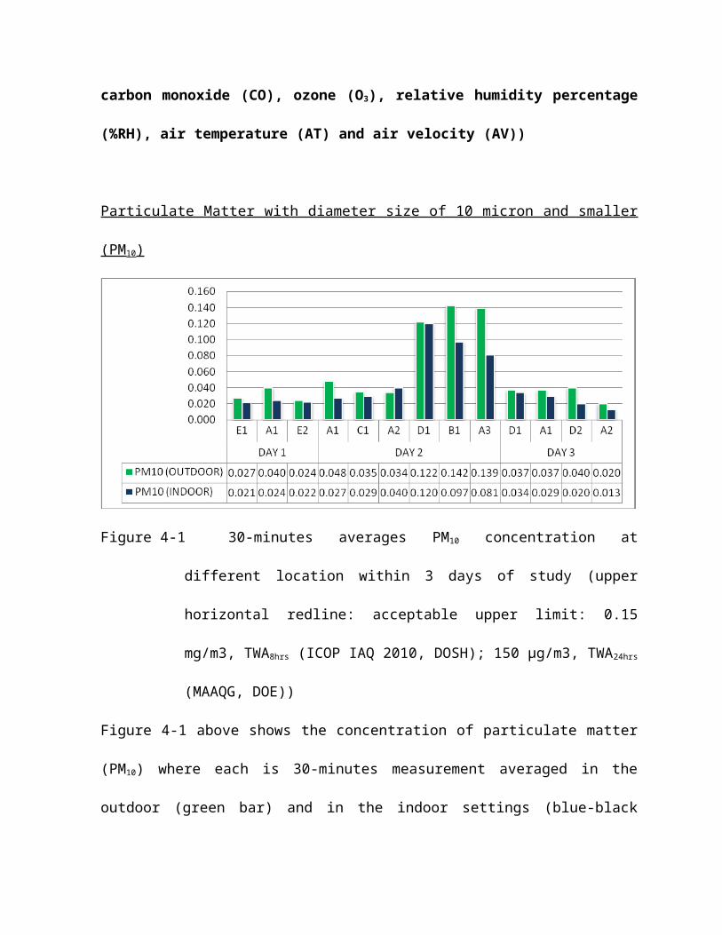
Figure 4-1 30-minutes averages PM10 concentration at different location within 3
days of study (upper horizontal redline: acceptable upper limit: 0.15
mg/m3, TWA8hrs (ICOP IAQ 2010, DOSH); 150 µg/m3, TWA24hrs
(MAAQG, DOE))

Figure 4-1 above shows the concentration of particulate matter (PM10) where each is
30-minutes measurement averaged in the outdoor (green bar) and in the indoor
settings (blue-black bar). Among all data captured, measurement done between
December 5, 2014 on 5.00 pm until 8.49 pm in the same day returned the highest
concentration compared to others, in both outdoor and indoor settings (column Day 2,
the first 3 sub-columns from the right (location D1, B1 and A3).
The highest concentration of PM10 in the outdoor is 0.142 mg/kg, captured on 30-
minutes measurement starting December 5, 2014 on 6.02 pm at the pillar between
Bay 06 and Bay 07 (column Day 2, location B1), followed by measurement started on
7.40 pm in the same day at the pillar between Bay 04 and Bay 05 (column Day 2,
location A3) with the concentration value of 0.139 mg/kg. Another data which can be
considered as higher is found during measurement started earlier at 5.02 pm in the
same day with value of 0.122 mg/kg. The measurement is done at the pillar between
Bay 10 and Bay 11 (column Day 2, location D1). From the observation during this
study, it is found that this fluctuation of the PM10 concentration is due to the increasing
number of heavy duty vehicle either park in or just crossed away, the inspection bays,
where it is estimated the total number of heavy duty vehicle is about 100 (40 bays X 2
heavy duty vehicles, plus with availability of 20 parking lots around the inspection
bays).

Except the obvious three higher concentrations as written above, other
concentrations for PM10 in the outdoor settings are scattered between the range of
0.020 mg/kg and 0.048 mg/kg. The lowest concentration for PM10 in the outdoor is
0.020 mg/kg which is measured at the pillar between Bay 04 and Bay 05 (column
Day 3, location A2) on December 7, 2014, started 7.50 pm.
In the indoor settings, the highest PM10 concentration is also found in same three
locations as in the outdoor (column Day 2, location D1, B1 and A2) within the same
period of the highest PM10 in the were outdoor found. However, the real highest PM10
value is found in inside the office of Bilik Sisihan Borang Kastam Import (column Day
2, location D1) with the concentration value of 0.120 mg/kg, on December 5, 2014
started at 5.44 pm. The concentration is decreased to 0.097 mg/kg inside the office of
Kaunter Pemeriksaan Kastam Import (column Day 2, location B1) which is started at
7.02 pm on the same day. About more than an hour later, the concentration of PM10
in the indoor settings is decreased to 0.081 mg/kg inside the office of Kaunter
Taksiran Kastam Import (column Day 2, location A3). In other locations within those 3
days, the concentration were found to be ranging from the lowest concentration value
of 0.013 mg/kg (column Day 3, location A2) which is measured on December 7, 2014
starting 8.27 pm; to the highest concentration value of 0.040 mg/kg (column Day 2,
location A2) which is measured on December 5, 2014 starting 9.35 am.
By referring Figure 4-1, it is found that the concentration of PM10 in the outdoor
settings are greater compared to the value of PM10 in the indoor settings at almost all
measurements done with the largest gap between both settings is in column Day 3,
location A3 which is measured on December 5, 2014 starting 7.40 pm with 41.727%
in differences, and smallest gap are found in column Day 1, location E2 which is
measured on December 4, 2014 starting 1.43 pm with the difference of 8.333%.
The only spot where I found the concentration value of PM10 in indoor settings is
greater than the concentration value in the outdoor is in column Day 2, location A2 on
December 5, 2014 starting at 11.36 am. During this measurement, I found the
concentration value of PM10 at the pillar between Bay 04 and Bay 05 is 0.034 mg/kg,
which is lesser than the concentration value of PM10 in the office of Kaunter Taksiran
Kastam Import where the value of PM10 found there is 0.040 mg/kg (slightly higher).
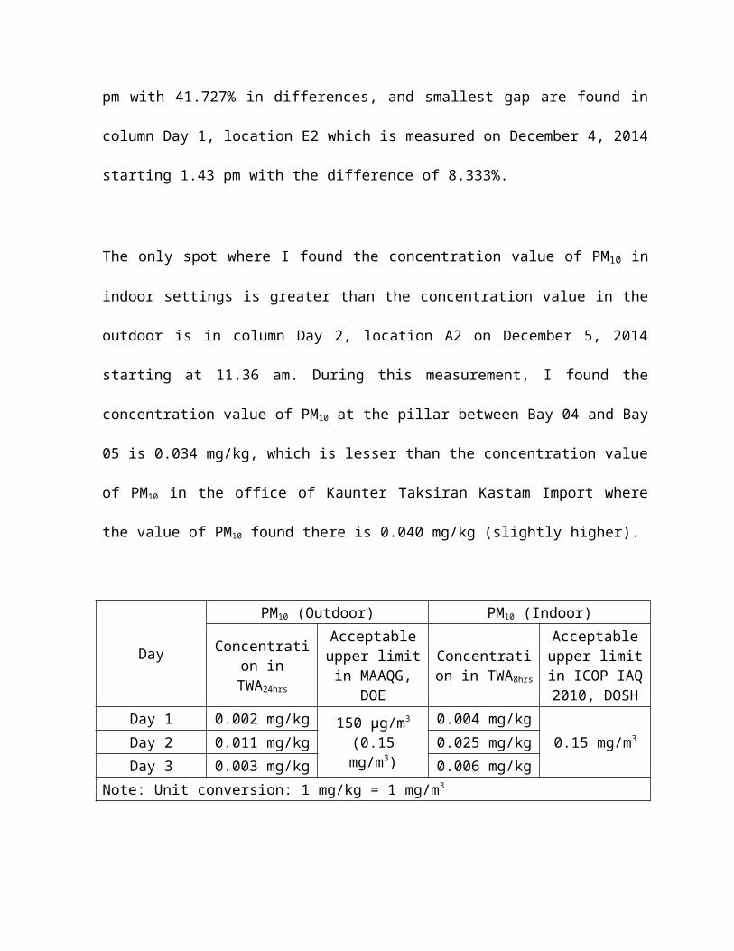
Day
PM10 (Outdoor) PM10 (Indoor)
Concentration in TWA24hrs
Acceptable upper limit in
MAAQG, DOE
Concentration in TWA8hrs
Acceptable upper limit in
ICOP IAQ 2010, DOSH
Day 1 0.002 mg/kg150 µg/m3
(0.15 mg/m3)
0.004 mg/kg0.15 mg/m3Day 2 0.011 mg/kg 0.025 mg/kg
Day 3 0.003 mg/kg 0.006 mg/kgNote: Unit conversion: 1 mg/kg = 1 mg/m3
Table 4-1 Results for each day TWA8hrs and TWA24hrs calculation from the PM10
concentration data obtained in Figure 4-1, and comparison with ICOP
IAQ 2010 and MAAQG, respectively.

Comparison between the data shown in Figure 4-1 after calculated for TWA8hrs and
TWA24hrs equivalent, for indoor and outdoor comparison with the related standards,
respectively, is as in Table 4-1 above.
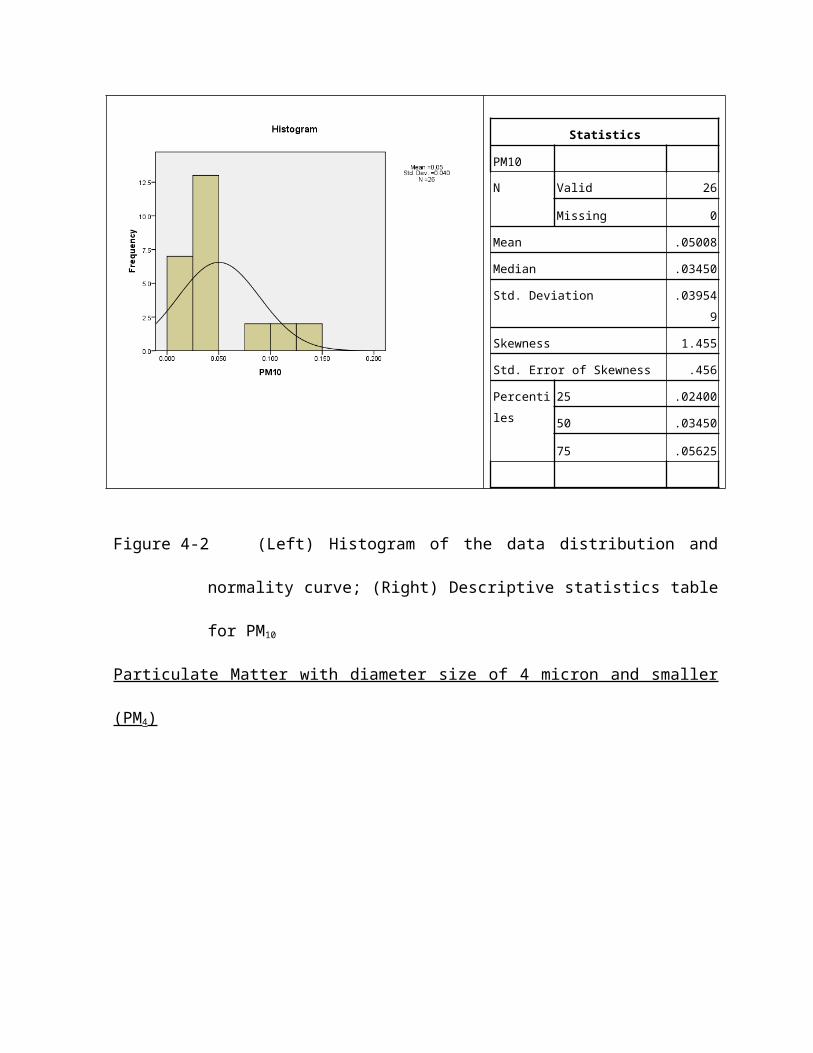
Using SPSS software, descriptive statistic analysis is conducted to evaluate the data
distribution normalities. As shown in Figure 4-2, it is found that the mean for PM 10
concentration is 0.05008 with standard deviation (SD) is 0.03450, while the median is
0.03450. For the histogram, it is found that the normality curve is skewed to the left
(positive skew). The distribution of the data is not normal.
Statistics
PM10
N Valid 26
Missing 0
Mean .05008
Median .03450
Std. Deviation .039549
Skewness 1.455
Std. Error of Skewness .456
Percentiles 25 .02400
50 .03450
75 .05625
Figure 4-2 (Left) Histogram of the data distribution and normality curve; (Right)
Descriptive statistics table for PM10
Particulate Matter with diameter size of 4 micron and smaller (PM4)
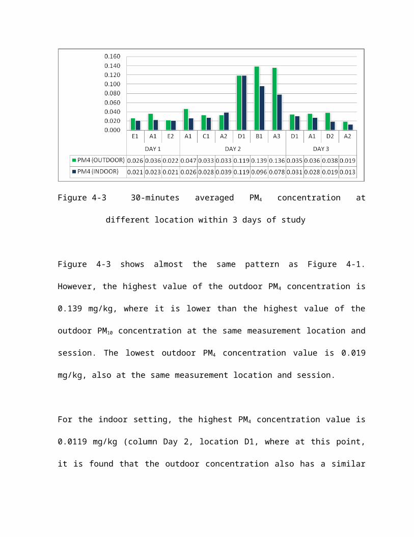
Figure 4-3 30-minutes averaged PM4 concentration at different location within 3
days of study
Figure 4-3 shows almost the same pattern as Figure 4-1. However, the highest value
of the outdoor PM4 concentration is 0.139 mg/kg, where it is lower than the highest
value of the outdoor PM10 concentration at the same measurement location and
session. The lowest outdoor PM4 concentration value is 0.019 mg/kg, also at the
same measurement location and session.
For the indoor setting, the highest PM4 concentration value is 0.0119 mg/kg (column
Day 2, location D1, where at this point, it is found that the outdoor concentration also
has a similar value), while the lowest PM4 concentration value is 0.013 mg/kg (column
Day 3, location A2).

At this moment, there is no suitable standard in Malaysia to be referred to compare
either the PM4 concentration found is comply or otherwise, both for ambient and
indoor air quality.
Statistics
PM4
N Valid 26
Missing 0
Mean .04850
Median .03300
Std. Deviation .039047
Skewness 1.464
Std. Error of Skewness .456
Percentiles 25 .02275
50 .03300
75 .05475
Figure 4-4 (Left) Histogram of the data distribution and normality curve; (Right)
Descriptive statistics table for PM4
Using SPSS software, descriptive statistic analysis is conducted to evaluate the data
distribution normalities. As shown in Figure 4-4 above, it is found that the mean for
PM4 concentration is 0.04850 with standard deviation (SD) is 0.039047, while the
median is 0.03300. For the histogram, it is found that the normality curve is skewed to
the left (positive skew). The distribution of the data is not normal.

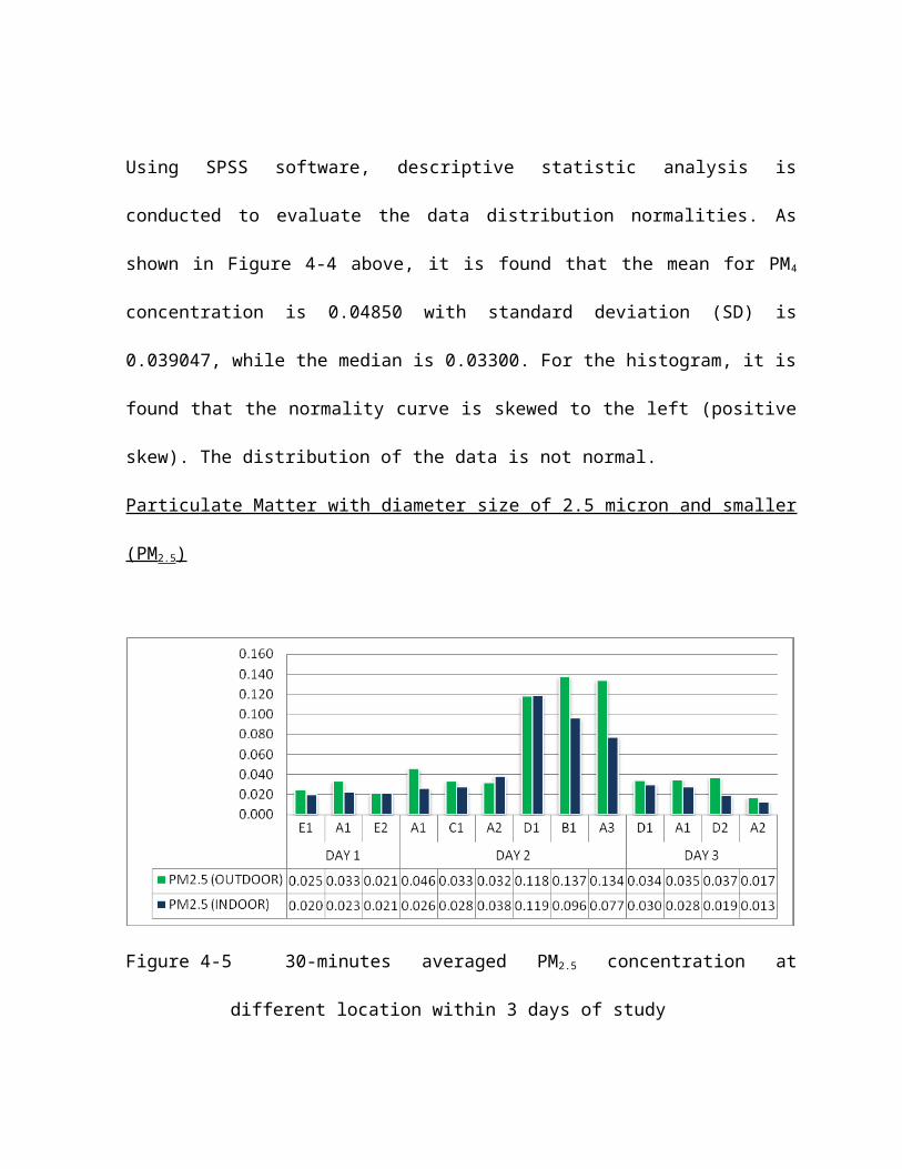
Particulate Matter with diameter size of 2.5 micron and smaller (PM2.5)
Figure 4-5 30-minutes averaged PM2.5 concentration at different location within 3
days of study
Figure 4-5 shows almost the same pattern as Figure 4-1. However, the highest value
of the outdoor PM2.5 concentration is 0.137 mg/kg, where it is lower than the highest
value of the outdoor PM10 concentration at the same measurement location and
session. The lowest outdoor PM2.5 concentration value is 0.017 mg/kg, also at the
same measurement location and session.
For the indoor setting, the highest PM2.5 concentration value is 0.0119 mg/kg (column
Day 2, location D1) while the lowest PM2.5 concentration value is 0.013 mg/kg
(column Day 3, location A2). In these two locations, data shown that there are no
differences in the highest and lowest concentration of PM2.5 and PM4. At the same

point as the highest concentration value of PM2.5 in indoor setting, the concentration
value for the outdoor is slightly lower.
At this moment, there is no suitable standard in Malaysia to be referred to compare
either the PM2.5 concentration found is comply or otherwise, both for ambient and
indoor air quality.
Statistics
PM2.5
N Valid 26
Missing 0
Mean .04769
Median .03250
Std. Deviation .038847
Skewness 1.460
Std. Error of Skewness .456
Percentiles 25 .02250
50 .03250
75 .05375
Figure 4-6 (Left) Histogram of the data distribution and normality curve; (Right)
Descriptive statistics table for PM2.5
Using SPSS software, descriptive statistic analysis is conducted to evaluate the data
distribution normalities. As shown in Figure 4-6 above, it is found that the mean for
PM2.5 concentration is 0.04769 with standard deviation (SD) is 0.038847, while the
median is 0.03250. For the histogram, it is found that the normality curve is skewed to
the left (positive skew). The distribution of the data is not normal.
Particulate Matter with diameter size of 1 micron and smaller (PM1)
Figure 4-7 30-minutes averaged PM1 concentration at different location within 3
days of study
Figure 4-7 shows almost the same pattern as Figure 4-1. However, the highest value
of the outdoor PM1 concentration is 0.131 mg/kg, where it is lower than the highest
value of the outdoor PM10 concentration at the same measurement location and
session. The lowest outdoor PM1 concentration value is 0.015 mg/kg, also at the
same measurement location and session.
For the indoor setting, the highest PM1 concentration value is 0.0116 mg/kg (column
Day 2, location D1) while the lowest PM1 concentration value is 0.013 mg/kg (column
Day 3, location A2).
It’s now obvious that there are three different spots where the outdoor PM1
concentration value is lower (or slightly lower) than the indoor PM1 concentration
value. Based on Figure 4-7, the locations are in column Day 1 (location E2), column
Day 2 (location A2) and column Day 2 (location D1).
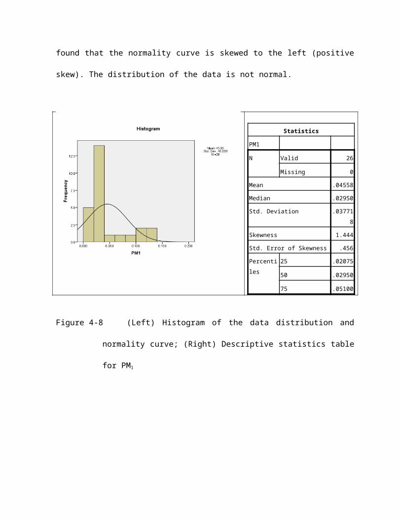
Using SPSS software, descriptive statistic analysis is conducted to evaluate the data
distribution normalities. As shown in Figure 4-8 below, it is found that the mean for
PM1 concentration is 0.04558 with standard deviation (SD) is 0.037718, while the
median is 0.02950. For the histogram, it is found that the normality curve is skewed to
the left (positive skew). The distribution of the data is not normal.

Statistics
PM1
N Valid 26
Missing 0
Mean .04558
Median .02950
Std. Deviation .037718
Skewness 1.444
Std. Error of Skewness .456
Percentiles 25 .02075
50 .02950
75 .05100
Figure 4-8 (Left) Histogram of the data distribution and normality curve; (Right)
Descriptive statistics table for PM1

Total Particulate Matter (PMTOTAL)
Figure 4-9 30-minutes averaged PMTOTAL concentration at different location within 3
days of study
Based on the Figure 4-9 above, the highest concentration value of PMTOTAL for
outdoor settings is found in column Day 2, location B1 (at the pillar between Bay 06
and Bay 07) which is measured on December 5, 2014 starts at 6.22 pm with the
concentration value of 0.144 mg/kg. For the indoor settings, the highest concentration
value of PMTOTAL is 0.124 mg/kg measured on December 5, 2014 starts at 5.02 pm in
column Day 2, location D1 (inside the office of Kaunter Pemeriksaan Import Kastam).
In this same spot, I found that the concentration value for outdoor setting (at the pillar
between Bay 10 and Bay 11) is the same.
The lowest concentration value for both indoor settings and outdoor settings is found
in column Day 3, location A2 measured on December 7, 2014 starting 7.50 pm and

ends at 8.57 pm. The concentration values are 0.021 mg/kg (outdoor) and 0.014
mg/kg (indoor).
The concentration value of PMTOTAL for indoor settings is appeared three times to be
higher or slightly higher than the PMTOTAL concentration value in outdoor settings. The
three locations are column Day 1, location E2 measured on December 4, 2014 starts
at 1.43 pm (indoor concentration value is 0.026 mg/kg (inside the office of Urusetia
Import Kastam, Seksyen Jaminan Bank) and outdoor concentration value at the pillar
between Bay 12 and Bay 13 is 0.025 mg/kg); column Day 2, location A2 which is
measured on December 5, 2014 starts at 11.36 am (indoor concentration value is
0.046 mg/kg (inside the office of Urusetia Taksiran Kastam Import) and the outdoor
concentration value at pillar between Bay 04 and Bay 05 is 0.035 mg/kg); and at
column Day 3, location D1 which measured on December 7, 2014 starts at 8.58 am
(indoor concentration value in the office of Bilik Sishan Borang Kastam Import is
0.040 mg/kg and outdoor concentration value at pillar between Bay 10 and Bay 11 is
0.037 mg/kg).
Using SPSS software, descriptive statistic analysis is conducted to evaluate the data
distribution normalities. As shown in Figure 4-10 below, it is found that the mean for
PMTOTAL concentration is 0.05288 with standard deviation (SD) is 0.040288, while the
median is 0.03650. For the histogram, it is found that the normality curve is skewed to
the left (positive skew). The distribution of the data is not normal.

Statistics
PM Total
N Valid 26
Missing 0
Mean .05288
Median .03650
Std. Deviation .040288
Skewness 1.400
Std. Error of Skewness .456
Percentiles 25 .02575
50 .03650
75 .06050
Figure 4-10 (Left) Histogram of the data distribution and normality curve; (Right)
Descriptive statistics table for PMTOTAL
Total Volatile Organic Compound (TVOC)
Figure 4-11 below shows the value of TVOC founds in the study locations. The
highest value for TVOC in the outdoor settings is found at the pillar between Bay 04
and Bay 05 with the concentration value is 38.97 ppm followed by slightly lower
concentration (38.96 ppm) found at the pillar between Bay 10 and Bay 11, both is
measured on December 7, 2014, starting from 6.04 pm. The lowest TVOC
concentration in outdoor settings is found at the pillar between Bay 10 and Bay 11
(2.13 ppm) measured on December 5, 2014 starts at 5.02 pm. For indoor settings,
the highest value is found on December 7, 2014 after measurement starts at 6.04 pm
in the office of Bilik Sisihan Borang Kastam Import (5.06 ppm). The lowest value of
indoor settings for TVOC is 1.21 ppm, measured in the office of Unit Taksiran Kastam
Import on December 7, 2014 starts at 1020 am.
Figure 4-11 30-minutes averaged TVOC concentration at different location within 3
days of study (the horizontal redline: acceptable upper limit: 3 ppm,
TWA8hrs (ICOP IAQ 2010, DOSH))
The values of TVOC are looks a like to be closer between indoor settings and
outdoor settings from the results obtained from measurement done on December 5,
2014 started 10.55 am until 7.32 pm (column Day 2, location C1 until location B1).
The values of TVOC in outdoor settings are ranged from 2.13 ppm and 2.99 ppm,
while the indoor settings TVOC value ranged from 1.16 ppm and 1.40 ppm.
Comparison between the data shown in Figure 4-11 after calculated for TWA8hrs
equivalent, for indoor TVOC concentration with the related standards, is as in Table
4-2 below.
DayTVOC (Indoor)
Concentration in TWA8hrs Acceptable upper limit in ICOP IAQ 2010, DOSHDay
1 0.593 ppm
3 ppmDay 2 0.553 ppm
Day 3 0.732 ppm
Table 4-2 Results for each day TWA8hrs calculation from the TVOC concentration
data obtained in Figure 4-11, and comparison with ICOP IAQ 2010
Statistics
TVOC
N Valid 26
Missing 0
Mean 7.4377
Median 3.0850
Std. Deviation 1.05511E1
Skewness 2.413
Std. Error of Skewness .456
Percentiles 25 1.9375
50 3.0850
75 7.4875
Figure 4-12 (Left) Histogram of the data distribution and normality curve; (Right)
Descriptive statistics table for TVOC
Using SPSS software, descriptive statistic analysis is conducted to evaluate the data
distribution normalities. As shown in Figure 4-12 below, it is found that the mean for
TVOC concentration is 7.4377 with standard deviation (SD) is 0.105511, while the
median is 3.0850. For the histogram, it is found that the normality curve is skewed to
the left (positive skew). The distribution of the data is not normal.
Carbon dioxide (CO2)
Figure 4-13 30-minutes averaged CO2 concentration at different location within 3
days of study (the horizontal redline: acceptable upper limit: C1000
ppm, TWA8hrs (ICOP IAQ 2010, DOSH))
As shown in Figure 4-13, at all time during this study conducted, CO2 values in the
indoor settings are higher compared to the CO2 values at the outdoor settings. The

highest CO2 value is 760 ppm measured in the indoor settings is in the office of Bilik
Sisihan Borang Kastam Import which is measured on December 5, 2014 started at
5.44 pm. At the same time, the value of CO2 at outdoor settings at the pillar between
Bay 10 and Bay 11 is 595 ppm. The highest CO2 value for outdoor settings is 606
ppm, measured on December 5, 2014 at 6.22 pm at the pillar between Bay 06 and
Bay 07, while the lowest CO2 value for both indoor and outdoor settings is measured
on December 7, 2014 started 7.50 pm until 8.57 pm with the value at the pillar
between Bay 04 and Bay 05 is 414 ppm and the value in the office of Unit Taksiran
Kastam Import is 531 ppm.
Comparison between the data shown in Figure 4-13 after calculated for TWA8hrs
equivalent, for indoor CO2 concentration with the related standards, is as in Table 4-3
below.
DayCO2 (Indoor)
Concentration in TWA8hrs Acceptable upper limit in ICOP IAQ 2010, DOSHDay
1 114.225 ppm
C1000 ppmDay 2 260.688 ppm
Day 3 145.438 ppm
Table 4-3 Results for each day TWA8hrs calculation from the CO2 concentration
data obtained in Figure 4-13, and comparison with ICOP IAQ 2010
Using SPSS software, descriptive statistic analysis is conducted to evaluate the data
distribution normalities. As shown in Figure 4-14 below, it is found that the mean for
carbon dioxide concentration is 575.65 with standard deviation (SD) is 90.324, while
the median is 574.00. For the histogram, it is found that the normality curve is slightly
skewed to the left (positive skew). The magnitude of the skewness is 0.291, which is
closer to the 0 (absolute normal distribution). The distribution of the data is slightly
normal.
Statistics
Carbon Dioxide
N Valid 26
Missing 0
Mean 575.65
Median 574.00
Std. Deviation 90.324
Skewness .291
Std. Error of Skewness .456
Percentiles 25 497.00
50 574.00
75 643.25
Figure 4-14 (Left) Histogram of the data distribution and normality curve; (Right)
Descriptive statistics table for carbon dioxide
Ozone (O3)
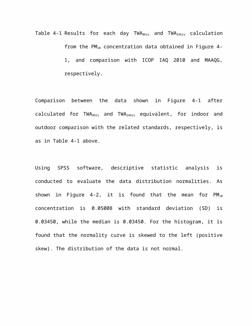
Figure 4-15 shows the ozone concentration value in both settings. The averaged
ozone concentration value for indoor settings are found only at two measurements
done December 5, 2014 started 5.02 pm until 7.32 pm in the office of Bilik Sisihan
Borang Kastam Import and in the office of Kaunter Pemeriksaan Kastam Import,
where the concentration value is same at 0.01 ppm. For outdoor settings, the value
of ozone is ranged from the lowest (0.00 ppm) until the highest (0.03 ppm).
Figure 4-15 30-minutes averaged ozone concentration at different location within 3
days of study (upper horizontal redline: acceptable upper limit: 0.05
ppm, TWA8hrs (ICOP IAQ 2010, DOSH); 0.06 ppm, TWA8hrs (MAAQG,
DOE))
Day
O3 (Outdoor) O3 (Indoor)
Concentration in TWA8hrs
Acceptable upper limit in
MAAQG, DOE
Concentration in TWA8hrs
Acceptable upper limit in
ICOP IAQ 2010, DOSH
Day 1 0.003 ppm 0.06 ppm 0.000 ppm 0.05 ppm
Day 2 0.004 ppm 0.001 ppmDay 3 0.002 ppm 0.000 ppm
Table 4-4 Results for each day TWA8hrs calculation from the ozone concentration
data obtained in Figure 4-15, and comparison with ICOP IAQ 2010 and
MAAQG, respectively.
Comparison between the data shown in Figure 4-15 after calculated for TWA8hrs
equivalent, for indoor and outdoor comparison with the related standards,
respectively, is as in Table 4-4 above.
Using SPSS software, descriptive statistic analysis is conducted to evaluate the data
distribution normalities. As shown in Figure 4-16 below, it is found that the mean for
ozone concentration is 0.0062 with standard deviation (SD) is 0.00941, while the
median is 0.0000. For the histogram, it is found that the normality curve is slightly
skewed to the left (positive skew). The magnitude of the skewness is 0.456, which is
closer to the 0 (absolute normal distribution). The distribution of the data is slightly
normal.
Statistics
Ozone
N Valid 26
Missing 0
Mean .0062
Median .0000
Std. Deviation .00941
Skewness 1.509
Std. Error of Skewness .456
Percentiles 25 .0000
50 .0000
75 .0100
Figure 4-16 (Left) Histogram of the data distribution and normality curve; (Right)
Descriptive statistics table for ozone
Carbon monoxide (CO)
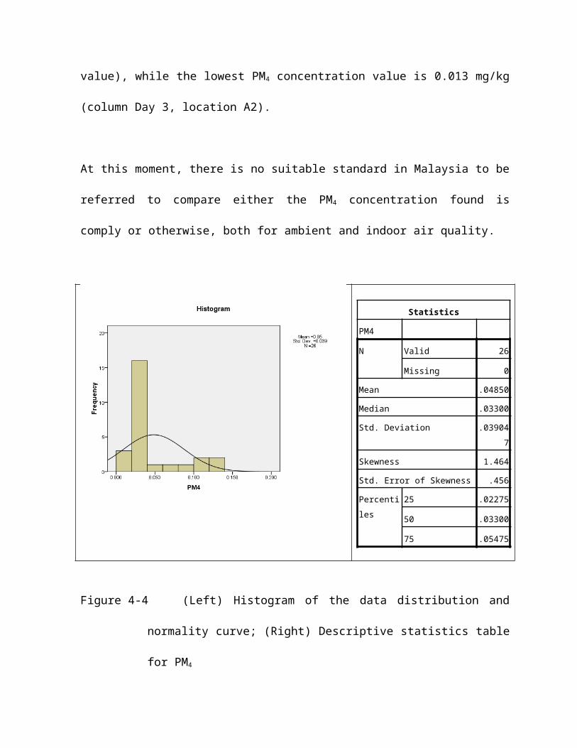
Figure 4-17 30-minutes averaged carbon monoxide concentration at different
location within 3 days of study (the horizontal redline: acceptable upper
limit: 10.0 ppm, TWA8hrs (ICOP IAQ 2010, DOSH); the horizontal purple
line 9.0 ppm, TWA8hrs (MAAQG, DOE))
The value of carbon monoxide concentration is shown in Figure 4-17 above. The
maximum value of CO is captured in column Day 1, location A1 on December 4, 2014
started from 12.14 pm until 1.33 pm for both indoor (in the office of Unit Taksiran
Kastam Import) and outdoor settings (at the pillar between Bay 04 and Bay 05). The
values are 17.3 ppm (outdoor settings) and 4.0 ppm (indoor settings). At all times
during this study, the value of CO for outdoor settings are higher compared to CO
value for indoor settings, except from December 5, 2014 started from 10.14 am until
6.14 pm, where the value for both settings is 0.0 ppm. Meanwhile, a measurement
done on December 5, 2014 started at 6.22 pm found that the value of CO in the
indoor settings (in the office of Kaunter Pemeriksaan Kastam Import: 0.1 ppm) is
slightly higher than the value of CO in the outdoor settings (at the pillar between Bay
06 and Bay 07: 0.0 ppm).
Day
CO (Outdoor) CO (Indoor)
Concentration in TWA8hrs
Acceptable upper limit in
MAAQG, DOE
Concentration in TWA8hrs
Acceptable upper limit in
ICOP IAQ 2010, DOSH
Day 1 2.206 ppm 9.0 ppm 0.334 ppm 10.0 ppm
Day 2 0.181 ppm 0.013 ppm
Day 3 1.181 ppm 0.119 ppm
Table 4-5 Results for each day TWA8hrs calculation from the CO concentration data
obtained in Figure 4-17, and comparison with ICOP IAQ 2010 and
MAAQG, respectively.
Comparison between the data shown in Figure 4-15 after calculated for TWA8hrs
equivalent, for indoor and outdoor comparison with the related standards,
respectively, is as in Table 4-5 above.
Using SPSS software, descriptive statistic analysis is conducted to evaluate the data
distribution normalities. As shown in Figure 4-18 below, it is found that the mean for
ozone concentration is 2.485 with standard deviation (SD) is 4.5509, while the
median is 0.500. For the histogram, it is found that the normality curve is skewed to
the left (positive skew). The magnitude of the skewness is 2.255, which is away from
absolute normal distribution. Therefore the distribution of the data is not normal.
Statistics
Carbon Monoxide
N Valid 26
Missing 0
Mean 2.485
Median .500
Std. Deviation 4.5509
Skewness 2.255
Std. Error of Skewness .456
Percentiles 25 .000
50 .500
75 2.575
Figure 4-18 (Left) Histogram of the data distribution and normality curve; (Right)
Descriptive statistics table for carbon monoxide
Air temperature (AT)
Based on Figure 4-19 below, the value of the air temperature in outdoor settings is
ranged between the lowest 23.0 ⁰C (at the pillar between Bay 05 and Bay 05) as
measured on December 7, 2014 started from 7.50 pm, and the highest 32.5 ⁰C (at
the pillar between Bay 06 and Bay 07) as measured on December 5, 2014 started
from 6.22 pm. The range of air temperature in indoor settings is from 21.7 ⁰C (in the
office of Unit Taksiran Kastam Import) as measured on December 7, 2014 started

from 7.50 pm, and the highest is 27.6 ⁰C (in the office of Bilik Sisihan Borang Kastam
Import) as measured on December 5, 2014 started from 5.44 pm.
Figure 4-19 30-minutes averaged air temperature at different location within 3 days
of study (the horizontal redline: acceptable range: 23.0 ⁰C – 26.0 ⁰C,
(ICOP IAQ 2010, DOSH))
Statistics
Air Temperature
N Valid 26
Missing 0
Mean 26.288
Median 26.000
Std. Deviation 2.9619
Skewness .465
Std. Error of Skewness .456
Percentiles 25 23.875
50 26.000
75 28.225

Figure 4-20 (Left) Histogram of the data distribution and normality curve; (Right)
Descriptive statistics table for air temperature
Using SPSS software, descriptive statistic analysis is conducted to evaluate the data
distribution normalities. As shown in Figure 4-20 above, it is found that the mean for
ozone concentration is 26.288 with standard deviation (SD) is 2.9619, while the
median is 26.000. For the histogram, it is found that the normality curve is slightly
skewed to the left (positive skew). The magnitude of the skewness is 0.465, which is
closer to absolute normal distribution (0). Therefore the distribution of the data is
slightly normal.
Relative humidity percentage (%RH)
Figure 4-21 30-minutes averaged relative humidity percentage at different location
within 3 days of study (the horizontal redline: acceptable range: 40 % –
70 % (ICOP IAQ 2010, DOSH))
As shown in Figure 4-21 above, it is found that the relative humidity percentage
(%RH) is higher in the outdoor setting compared to the indoor setting. The maximum
value of %RH is 97.9%. The %RH value is found to be more than 80.0% during rainy
day or slightly after, while the %RH value is found more than 90.0% during heavy rain
day. The minimum value of %RH is 48.4%.
Statistics
Relative Humidity
N Valid 26
Missing 0
Mean 68.885
Median 64.800
Std. Deviation 14.8105
Skewness .665
Std. Error of Skewness .456
Percentiles 25 57.825
50 64.800
75 77.400
Figure 4-22 (Left) Histogram of the %RH data distribution and normality curve;
(Right) Descriptive statistics table for %RH
Using SPSS software, descriptive statistic analysis is conducted to evaluate the data
distribution normalities. As shown in Figure 4-22 above, it is found that the mean for
ozone concentration is 68.885 with standard deviation (SD) is 14.8105, while the
median is 64.800. For the histogram, it is found that the normality curve is slightly
skewed to the left (positive skew). The magnitude of the skewness is 0.665, which is
closer to absolute normal distribution (0). Therefore the distribution of the data is
slightly normal.
Air velocity (AV)
Figure 4-23 30-minutes averaged air velocity at different location within 3 days of
study (the horizontal redline: acceptable range: 0.15 m/s – 0.50 m/s
(ICOP IAQ 2010, DOSH))

Based on Figure 4-23, the air velocity for outdoor settings is ranged from the slowest
(0.05 m/s) to the fastest (22.6 m/s) while the air velocity for indoor setting is ranged
from the slowest (0.00 m/s) to the highest (0.29 m/s). At average of all time, the
velocity is higher in the outdoor settings compared to the indoor settings.
Using SPSS software, descriptive statistic analysis is conducted to evaluate the data
distribution normalities. As shown in Figure 4-24 below, it is found that the mean for
ozone concentration is 1.030 with standard deviation (SD) is 4.4040, while the
median is 0.070. For the histogram, it is found that the normality curve is skewed to
the left (positive skew). Therefore the distribution of the data is slightly normal.
Statistics
Air
Velocity
N Valid 26
Missing 0
Mean 1.030
Median .070
Std. Deviation 4.4040
Skewness 5.082
Std. Error of Skewness .456
Percentiles 25 .018
50 .070
75 .295
Figure 4-24 (Left) Histogram of the air velocity data distribution and normality curve;
(Right) Descriptive statistics table for air velocity
Conclusion for the result of specific objective (1)
Using the monitoring instruments as declared in Chapter 3 for in-situ air quality
measurement in both outdoor and indoor settings, the specific objective (1) is fulfilled
for the listed air quality parameters. In all three days of monitoring, 26 sampling
activities has been in ten different locations which have been visited (outdoor –
inspection bay; and indoor - offices) at the Import Lane of KSAB.
The focused parameter, particulate matters, especially PM10 has been found not
violating the standards (MAAQG and ICOP IAQ 2010), either during the 30-minutes
averaged measurement or after been calculated for TWA8hrs and TWA24hrs, for indoor
air quality and ambient air quality, respectively. The particulate matter concentration
is seems to be higher in both settings as influenced by the increasing number of
heavy duty vehicles either crossed-by or parked at the inspection bay.
By using descriptive statistic analysis, it is found that all of the data are not normally
distributed, although some parameters showing skewness is below +1.0 and slightly
closed to the 0 (the closest value of skewness is about +0.2). Therefore, in further
analysis of determining the significant different between indoor and outdoor, non-
parametric analysis will be more suitable instead of using t-test.
Specific objective (2): to compare the particulate matters concentration
between the outdoor and indoor settings
As all of the data have positive skewness with value of more than 0, significant
different analysis is done using Kruskal-Wallis Non-Parametric Test (Kruskal-Wallis H
Test) using SPSS version 16.0. This is alternative test for One-way ANOVA is data is
distributed normally. Location setting is set for grouping variable, which the group is
defined as 1 (outdoor setting) and 2 (indoor setting). The output result generated as
follow:
Descriptive Statistics
N Mean Std. Deviation Minimum Maximum
Percentiles
25th 50th (Median) 75th
PM10 26 .05008 .039549 .013 .142 .02400 .03450 .05625
PM4 26 .04850 .039047 .013 .139 .02275 .03300 .05475
PM2.5 26 .04769 .038847 .013 .137 .02250 .03250 .05375
PM1 26 .04558 .037718 .012 .131 .02075 .02950 .05100
PM Total 26 .05288 .040288 .014 .144 .02575 .03650 .06050
TVOC 26 7.4377 10.55112 1.16 38.97 1.9375 3.0850 7.4875
Carbon Dioxide 26 575.65 90.324 414 760 497.00 574.00 643.25
Ozone 26 .0062 .00941 .00 .03 .0000 .0000 .0100
Carbon
Monoxide26 2.485 4.5509 .0 17.3 .000 .500 2.575
Air Temperature 26 26.288 2.9619 21.7 32.5 23.875 26.000 28.225
Relative Humidity 26 68.885 14.8105 48.4 97.9 57.825 64.800 77.400
Air Velocity 26 1.030 4.4040 .0 22.6 .018 .070 .295
Location Setting 26 1.50 .510 1 2 1.00 1.50 2.00
Table 4-6 Output results for descriptive statistics after analysis of Kruskal-Wallis
Non-Parametric Test (K-Independent Sample) has been run in SPSS.
Ranks
Location Setting N Mean Rank
PM10 Outdoor Setting 13 15.85
Indoor Setting 13 11.15
Total 26
PM4 Outdoor Setting 13 15.73Indoor Setting 13 11.27Total 26
PM2.5 Outdoor Setting 13 15.58Indoor Setting 13 11.42Total 26
PM1 Outdoor Setting 13 15.42Indoor Setting 13 11.58Total 26
PM Total Outdoor Setting 13 15.31Indoor Setting 13 11.69Total 26
TVOC Outdoor Setting 13 18.38Indoor Setting 13 8.62Total 26
Carbon Dioxide Outdoor Setting 13 7.85Indoor Setting 13 19.15Total 26
Ozone Outdoor Setting 13 16.81Indoor Setting 13 10.19Total 26
Carbon Monoxide Outdoor Setting 13 16.12Indoor Setting 13 10.88Total 26
Air Temperature Outdoor Setting 13 16.69Indoor Setting 13 10.31Total 26
Relative Humidity Outdoor Setting 13 18.46Indoor Setting 13 8.54Total 26
Air Velocity Outdoor Setting 13 19.35
Indoor Setting 13 7.65
Total 26
Table 4-7 Output results for the Mean Rank
Test Statisticsa,b
PM10 PM4 PM2.5 PM1 PM
Total
TVOC Carbon
Dioxide
Ozone Carbon
Monoxide
Air
Temperature
Relative
Humidity
Air
Velocity
Chi-
Square2.455 2.217 1.919 1.648 1.456
10.60
414.212 6.442 3.175 4.534 10.941 15.258
df 1 1 1 1 1 1 1 1 1 1 1 1
Asymp.
Sig..117 .136 .166 .199 .228 .001 .000 .011 .075 .033 .001 .000
a. Kruskal Wallis Testb. Grouping Variable: Location Setting
Table 4-8 Output results for the Test Statistics (Chi-Square, X2)
Frequencies
Location Setting
Outdoor Setting Indoor Setting
PM10 > Median 9 4
<= Median 4 9PM4 > Median 8 4

<= Median 5 9PM2.5 > Median 9 4
<= Median 4 9PM1 > Median 9 4
<= Median 4 9PM Total > Median 8 5
<= Median 5 8TVOC > Median 9 4
<= Median 4 9Carbon Dioxide > Median 2 11
<= Median 11 2Ozone > Median 8 2
<= Median 5 11Carbon Monoxide > Median 9 4
<= Median 4 9Air Temperature > Median 8 5
<= Median 5 8Relative Humidity > Median 11 2
<= Median 2 11Air Velocity > Median 12 1
<= Median 1 12
Table 4-9 Output results for the FrequencyTest Statisticsa
PM10 PM4 PM2.5 PM1 PM
Total
TVOC Carbon
Dioxide
Ozone Carbon
Monoxide
Air
Temperature
Relative
Humidity
Air
Velocity
N 26 26 26 26 26 26 26 26 26 26 26 26
Median .03450 .03300 .03250 .02950 .03650 3.0850 574.00 .0000 .500 26.000 64.800 .070
Exact
Sig..115 .238 .115 .115 .434 .115 .001 .041 .115 .434 .001 .000
a. Grouping Variable: Location Setting
Table 4-10 Output results for the Test Statistics (median)
Conclusion from the result obtained in fulfilling the specific objective (2):

Based on Table 4-8 above, it is found that there are statistically significant differences
found between the location settings and (1) TVOC (X2(1)=10.604, p=0.001, with
mean rank TVOC of 18.38 for the outdoor and 8.62 for the indoor setting); (2) carbon
dioxide (X2(1)=14.212, p=0.000, with mean rank carbon dioxide of 7.85 for the
outdoor and 19.15 for the indoor setting); (3) relative humidity (X2(1)=10.941,
p=0.001, with mean rank relative humidity of 18.46 for the outdoor and 8.54 for the
indoor setting); and (4) air velocity (X2(1)=15.258, p=0.000, with mean rank air
velocity of 19.35 for the outdoor and 7.65 for the indoor setting).
For the focused parameters in this study, particulate matters, it is found that there are
no statistically significant differences between location settings and particulate
matters: (1) PM10 (X2(1)=2.455, p=0.117, with mean rank PM10 of 15.85 for the
outdoor and 11.15 for the indoor setting); (2) PM4 (X2(1)=2.217, p=0.136, with mean
rank PM4 of 15.73 for the outdoor and 11.27 for the indoor setting); (3) PM2.5
(X2(1)=1.919, p=0.166, with mean rank PM2.5 of 15.58 for the outdoor and 11.42 for
the indoor setting); (4) PM1 (X2(1)=1.648, p=0.199, with mean rank PM1 of 15.42 for
the outdoor and 11.58 for the indoor setting); and (5) PMTOTAL (X2(1)=1.456, p=0.228,
with mean rank PMTOTAL of 15.31 for the outdoor and 11.69 for the indoor setting).
Ozone concentration, carbon monoxide and air temperature are also found not
statistically significant different with the location settings, outdoor and indoor,
respectively.
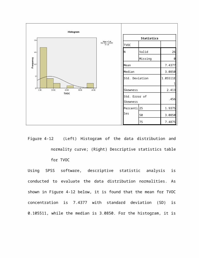
For particulate matter, it is found that the gap of differences of particulate
concentration and location settings is become larger when the diameter size of the
particulate matters become smaller (p-value ranged from 0.117 for PM10 to 0.199 for
PM1), while based on the mean rank, the concentration become lesser the diameter
size of the particulate matter become smaller for the outdoor (from 15.85 for PM10 to
15.42 for PM1), but vice-versa for the indoor setting (from 11.15 for PM10 to 11.58 for
PM1).
Hypothesis testing for objective (2):
H0: μA ≠ μB (p < 0.005) HA: μA = μB (p < 0.005)
It is found that p-value > 0.005 for particulate matter, thus accept HA.
Specific objective (3): to identify the relationship between particulate matter
and other parameters in the outdoor and in the indoor settings
Spearman’s Non-Parametric Correlation Test is used to analyse the correlation
between particulate matters concentration and the other air quality parameters.
Correlations
PM10 PM4 PM2.5 PM1 PM Total
Spearman's rho TVOC Correlation Coefficient -.176 -.198 -.213 -.244 -.215
Sig. (2-tailed) .391 .333 .295 .230 .291
N 26 26 26 26 26
Carbon Dioxide Correlation Coefficient .248 .262 .290 .307 .304
Sig. (2-tailed) .222 .196 .151 .128 .131
N 26 26 26 26 26
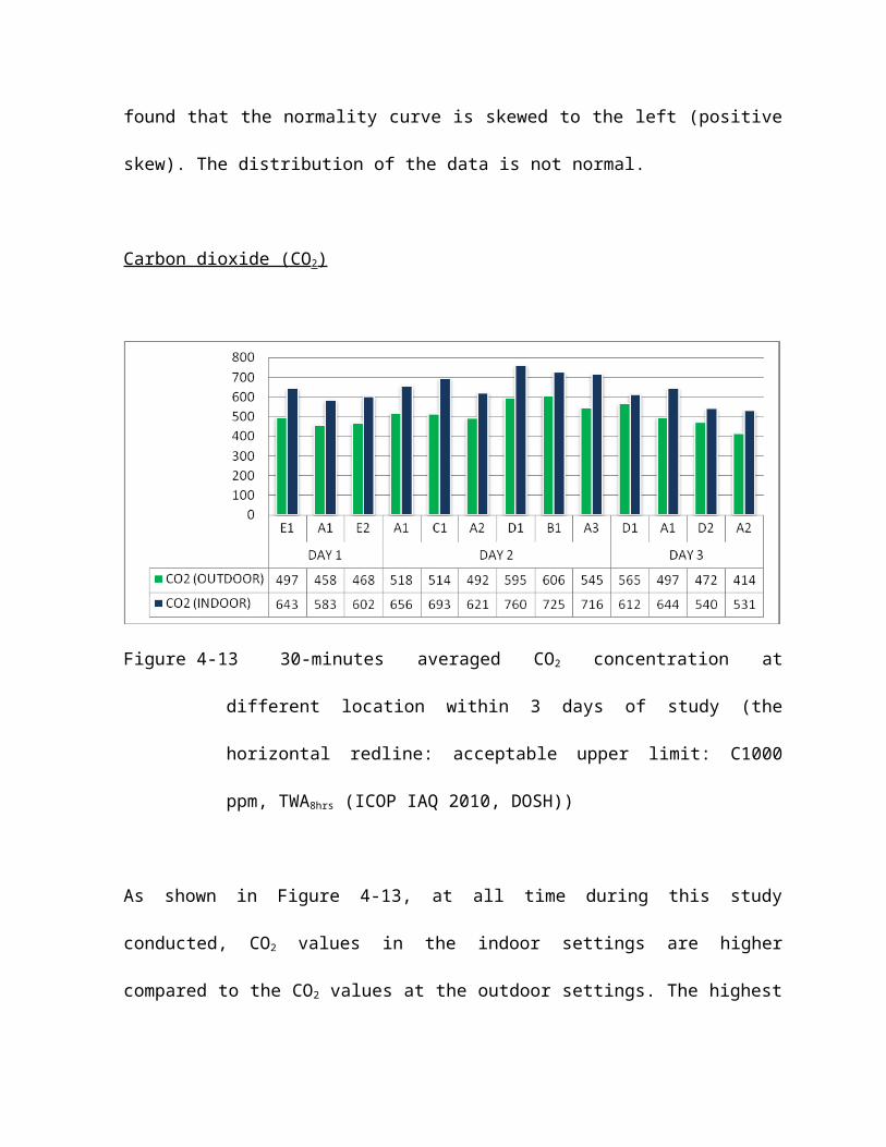
Ozone Correlation Coefficient .341 .325 .280 .253 .309
Sig. (2-tailed) .089 .105 .165 .213 .125
N 26 26 26 26 26
Carbon Monoxide Correlation Coefficient -.377 -.400* -.428* -.479* -.410*
Sig. (2-tailed) .057 .043 .029 .013 .037
N 26 26 26 26 26
Air Temperature Correlation Coefficient .682** .688** .706** .724** .657**
Sig. (2-tailed) .000 .000 .000 .000 .000
N 26 26 26 26 26
Relative Humidity Correlation Coefficient -.210 -.229 -.253 -.282 -.263
Sig. (2-tailed) .303 .260 .212 .163 .194
N 26 26 26 26 26
Air Velocity Correlation Coefficient .339 .344 .333 .334 .264
Sig. (2-tailed) .090 .085 .097 .095 .192
N 26 26 26 26 26
**. Correlation is significant at the 0.01 level (2-tailed).
*. Correlation is significant at the 0.05 level (2-tailed).
Table 4-11 Spearman’s correlation output results. The table is been simplified to fit
the page
From the Spearman’s rank-order correlation output (which the table has been
simplified to suit the page), the correlation between particulate matters (each type)
and the other air quality parameters are obtained.
There are strong, positive correlations between each type of particulate matter and
air temperature, which are statistically significant (PM10: rs(24)=.682, p=.000; PM4:
rs(24)=.688, p=.000; PM2.5: rs(24)=.706, p=.000; PM1: rs(24)=.724, p=.000; and
PMTOTAL: rs(24)=.657, p=.000).
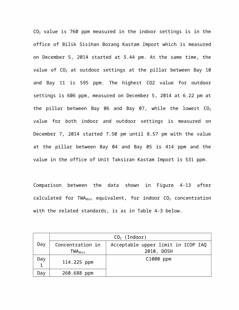
Between each type particulate matters and TVOC, as well as with relative humidity,
the correlation is weak and negative. The other parameter which has negative
correlation with each type of particulate matters is carbon monoxide. However, it is a
moderate correlation, not weak.
Between each type particulate matters and carbon dioxide, the correlation is positive,
ranged from weak to slightly moderate as according to the particulate diameter size
from smaller to larger. However, with the ozone, the correlation is also positive but
the strength of the correlation is from moderate to weak as according to the
particulate diameter size. With air velocity, the correlation is moderate and positive.
However, except for correlation between each type of particulate matter and air
temperature, all other correlations are not statistically significant.
Hypothesis testing for objective (3):
H0: rA = rB (p < 0.005) HA: rA ≠ rB (p > 0.005)
It is found that p-value < 0.005 only for correlation between particulate matter
and carbon dioxide, thus accept H0 for correlation with carbon dioxide, but the
p-value > 0.005 for particulate matter correlation with other pollutants,
therefore reject H0 for correlation between particulate matters and other
pollutants.
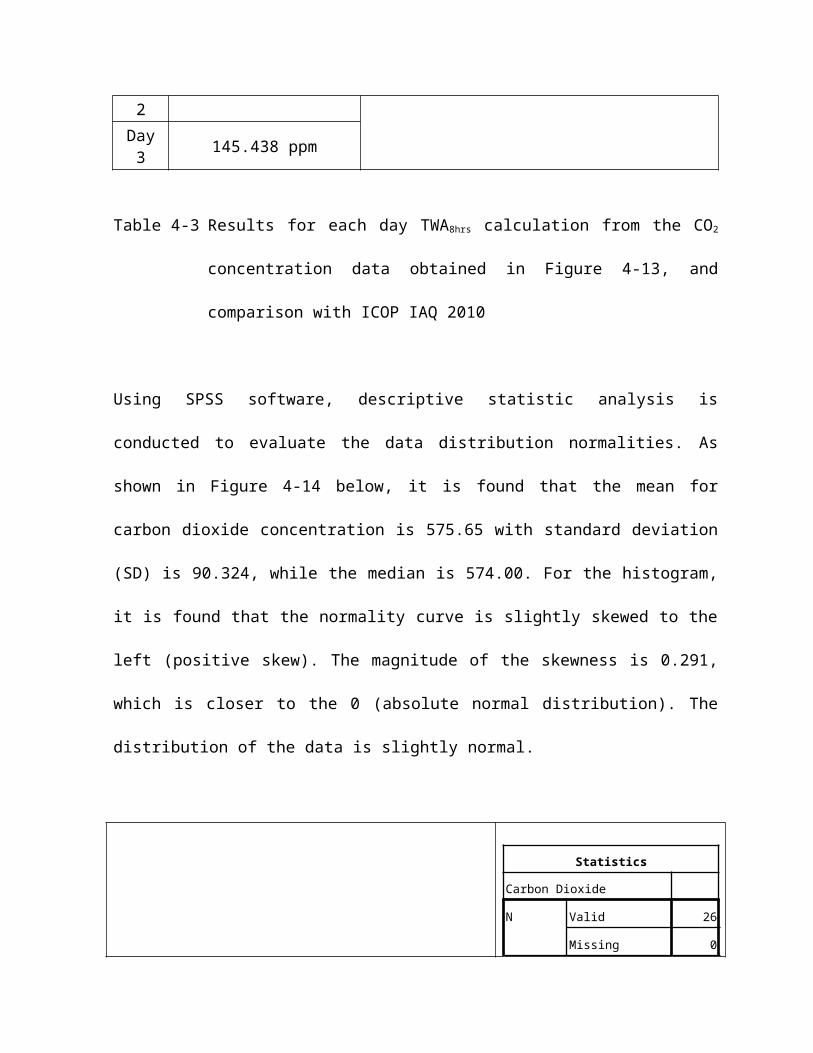
Specific objective (4): to calculate particulate matter indoor-outdoor (I/O) ratio
The formula for indoor-outdoor ratio is as follow:
I/Ox =Indoor particulate matter concentration (PMx)
Outdoor particulate matter concentration (PMx)
where x is category of particulate matter, which is 10, 4, 2.5 and 1
The I/O ratio calculation will be used the mean value for each concentration in the
specific location settings.
Statistics
PM10
Outdoor
PM10
Indoor
PM4
Outdoor
PM4
Indoor
PM2.5
Outdoor
PM2.5
Indoor
PM1
Outdoor
PM1
Indoor
PM Total
Outdoor
PM Total
Indoor
N Valid 13 13 13 13 13 13 13 13 13 13
Missing 0 0 0 0 0 0 0 0 0 0
Mean .05731 .04285 .05531 .04169 .05400 .04138 .05108 .04008 .05892 .04685
Median .03700 .02900 .03600 .02800 .03400 .02800 .03300 .02700 .03900 .03100
Std. Deviation.044724 .033840 .044141
.03357
9.043936 .033577 .042567
.03296
1.045383 .035256
Variance .002 .001 .002 .001 .002 .001 .002 .001 .002 .001
Minimum .020 .013 .019 .013 .017 .013 .015 .012 .021 .014
Maximum .142 .120 .139 .119 .137 .119 .131 .116 .144 .124

Table 4-12 Descriptive statistics output when the concentration of particulate matter
is separated in specific location settings with N=13 for each setting
Therefore:
I/O ratio for particulate matter (PM10):
I/O10 =Mean of overall indoor particulate matter (PM10)
Mean of overall outdoor particulate matter (PM10)
I/O10 =0.04285
0.05731
I/O10 = 0.748
For PM10, the I/O ratio is indicates from this study the indoor concentration of PM10 is
74.8% of the outdoor concentration of PM10
I/O ratio for particulate matter (PM4):
I/O4 =Mean of overall indoor particulate matter (PM4)
Mean of overall outdoor particulate matter (PM4)
I/O4 =0.04169
0.05531
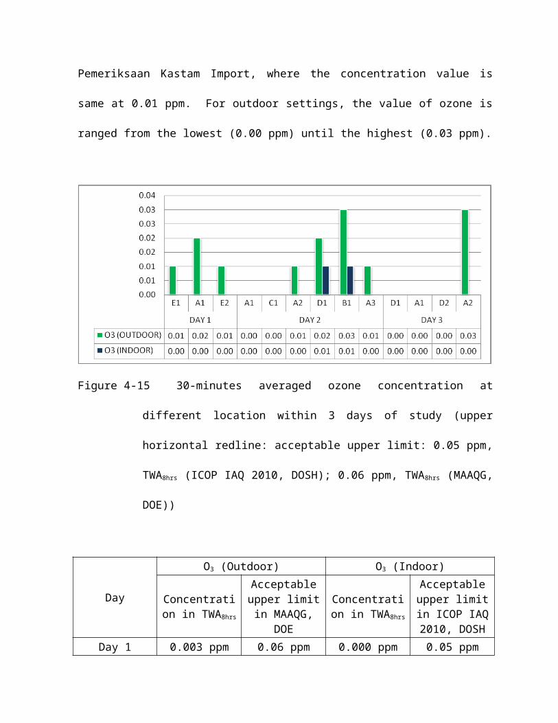
I/O4 = 0.754
For PM4, the I/O ratio is indicates from this study the indoor concentration of PM4 is
75.4% of the outdoor concentration of PM4
I/O ratio for particulate matter (PM2.5):
I/O2.5 =Mean of overall indoor particulate matter (PM2.5)
Mean of overall outdoor particulate matter (PM2.5)
I/O2.5 =0.04138
0.05400
I/O2.5 = 0.766
For PM2.5, the I/O ratio is indicates from this study the indoor concentration of PM2.5 is
76.6% of the outdoor concentration of PM2.5
I/O ratio for particulate matter (PM1):
I/O1 =Mean of overall indoor particulate matter (PM1)
Mean of overall outdoor particulate matter (PM1)
I/O1 =0.04008
0.05108
I/O1 = 0.785
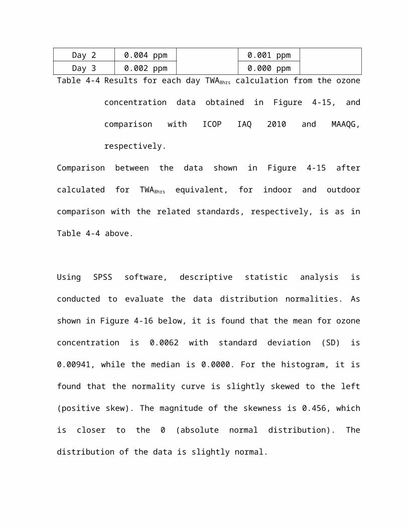
For PM1, the I/O ratio is indicates from this study the indoor concentration of PM1 is
78.5% of the outdoor concentration of PM1
I/O ratio for particulate matter (PMTOTAL):
I/OTOTAL =Mean of overall indoor particulate matter (PMTOTAL)
Mean of overall outdoor particulate matter (PMTOTAL)
I/OTOTAL =0.04685
0.05892
I/OTOTAL = 0.795
For PMTOTAL, the I/O ratio is indicates from this study the indoor concentration of
PMTOTAL is 79.49% of the outdoor concentration of PMTOTAL
Hypothesis testing for objective (4):
H0: I/OPM < 1 HA: I/OPM > 1
It is found that I/OPM < 1 therefore accept H0. However, the degree 20% in
difference can be considered as small, thus this hypothesis may not be
conflicting the hypothesis for specific objective (2).
CHAPTER FIVE
DISCUSSION
By referring to Figure 4-1, Figure 4-3, Figure 4-5, Figure 4-7 and Figure 4-9, all types
of particulate matter concentrations have almost the same pattern of exposures. The
highest peak for particulate matter exposure in outdoor settings, based on those
figures is at pillar between Bay 06 and Bay 07 measured on December 5, 2014
started at 6.22 pm until 6.52 pm (column Day 2, location B1) (PM 10 = 0.142 mg/kg,
PM4 = 0.139 mg/kg, PM2.5 = 0.137 mg/kg, PM1 = 0.131 mg/kg, PMTOTAL = 0.144
mg/kg), while the lowest particulate matter exposure in outdoor settings, based on the
figures is at pillar between Bay 04 and Bay 05 measured on December 7, 2014
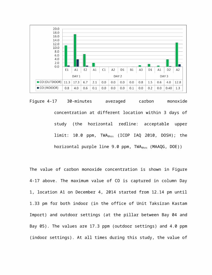
started at 7.50 pm until 8.20 pm (column Day 3, location A2) (PM 10 = 0.020 mg/kg,
PM4 = 0.019 mg/kg, PM2.5 = 0.017 mg/kg, PM1 = 0.015 mg/kg, PMTOTAL = 0.021
mg/kg).
For particulate matter exposure in indoor settings, the highest peak is found during
the measurement done inside the office of Bilik Sisihan Borang Kastam Import
measured on December 5, 2014 started at 5.44 pm until 6.14 pm (column Day 2,
location D1) (PM10 = 0.122 mg/kg, PM4 = 0.119 mg/kg, PM2.5 = 0.118 mg/kg, PM1 =
0.113 mg/kg, PMTOTAL = 0.124 mg/kg), while the lowest exposure found during
measurement inside the office of Kaunter Taksiran Kastam Import measured on
December 7, 2014 started at 8.27 pm until 8.57 pm (column Day 3, location A2) (PM10
= 0.013 mg/kg, PM4 = 0.013 mg/kg, PM2.5 = 0.013 mg/kg, PM1 = 0.012 mg/kg, PMTOTAL
= 0.014 mg/kg).
Based on these figures, it is found that at all time, the particulate matter exposures
are higher at the outdoor settings compared to indoor settings, except during
measurement done in column Day 2, location A2 on December 5, 2014 started on
11.36 am until 12.41 pm, the particulate matter exposure in outdoor settings is lower
than the particulate matter in indoor settings (PM10in, PM10out = 0.040 mg/kg, 0.034
mg/kg; PM4in, PM4out = 0.039 mg/kg, 0.033 mg/kg; PM2.5in, PM2.5out = 0.038 mg/kg,
0.032 mg/kg; PM1in, PM1out = 0.037 mg/kg, 0.030 mg/kg; PMTOTALin, PMTOTALout = 0.046
mg/kg, 0.035 mg/kg). Based on my observation, during the 30-minutes measurement,
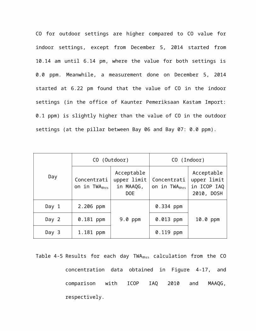
the period of the door which is opposite to the inspection bay left opened was about
11 minutes, whiles the frequency of the door opened and closed is 8 times.
As for general, according to Grau-Bove & Strlic (2013), the indoor particulate matter
concentration is generally a reflection of the outdoor concentration. However, when
there are sources of contamination such as wood burner, cooking stove or even
smoking activities, the concentration of the indoor settings may be higher than the
concentration of the outdoor settings.
From Table 4-10, it is found that the only air quality parameter which is significantly
correlated with particulate matter is air temperature. The strong, positive correlation
reflects that when there is small difference (increment) in air temperature it will
influence the huge increment in particulate matters concentration.
Thus, a calculation to determining the size of gap between the indoor and outdoor
value of the temperature and other particulate matters at each sampling location is
done. From the result, smaller differences between indoor and outdoor air
temperature promote higher number of I/O ratio.
For other parameters, it is learnt that the value of total volatile organic compound
(TVOC), carbon monoxide (CO), ozone (O3), temperature, relative humidity and air
speed are also higher at the outdoor settings rather than in indoor settings. However,
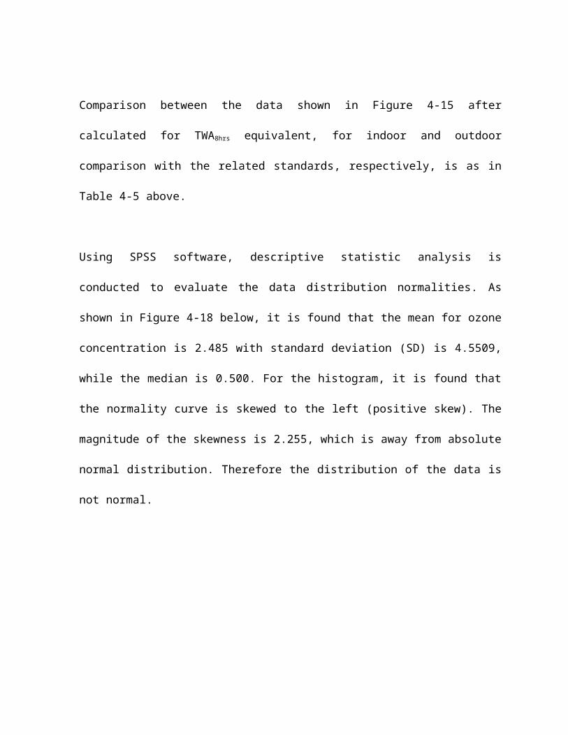
only the value of carbon dioxide (CO2) is found higher in indoor settings compared to
the outdoor settings at all time.
As all of the data have positive skewness with value of more than 0, significant
different analysis is done using Kruskal-Wallis Non-Parametric Test (Kruskal-Wallis H
Test). The result shows that there are no statistically significant differences between
the outdoor and the indoor concentration of particulate matters, ozone, carbon
monoxide and air temperature. However there are statistically significant differences
in TVOC and carbon dioxide concentrations, as well as in relative humidity
percentage and air velocity (p < 0.005).
For particulate matter, it is found that the gap of differences of particulate
concentration and location settings is become larger when the diameter size of the
particulate matters become smaller (p-value ranged from 0.117 for PM10 to 0.199 for
PM1), while based on the mean rank, the concentration become lesser the diameter
size of the particulate matter become smaller for the outdoor (from 15.85 for PM10 to
15.42 for PM1), but vice-versa for the indoor setting (from 11.15 for PM10 to 11.58 for
PM1).
To understand relationship and correlation between each category of particulate
matters and other parameter, a Spearman’s correlation analysis has been done.
From the Spearman’s rank-order correlation output (which the table has been
simplified to suit the page), the correlation between particulate matters (each type)
and the other air quality parameters are obtained.
There are strong, positive correlations between each type of particulate matter and
air temperature, which are statistically significant (PM10: rs(24)=.682, p=.000; PM4:
rs(24)=.688, p=.000; PM2.5: rs(24)=.706, p=.000; PM1: rs(24)=.724, p=.000; and
PMTOTAL: rs(24)=.657, p=.000).
Between each type particulate matters and TVOC, as well as with relative humidity,
the correlation is weak and negative. The other parameter which has negative
correlation with each type of particulate matters is carbon monoxide. However, it is a
moderate correlation, not weak.
Between each type particulate matters and carbon dioxide, the correlation is positive,
ranged from weak to slightly moderate as according to the particulate diameter size
from smaller to larger. However, with the ozone, the correlation is also positive but
the strength of the correlation is from moderate to weak as according to the
particulate diameter size. With air velocity, the correlation is moderate and positive.
However, except for correlation between each type of particulate matter and air
temperature, all other correlations are not statistically significant.

Indoor-Outdoor (I/O) Ratio
From the calculation conducted, it is found that the ratios are as follow:
I/O for PM10 = 0.748
I/O for PM4 = 0.754
I/O for PM2.5= 0.766
I/O for PM1 = 0.785
I/O for PMTOTAL = 0.795
The concentration of all type particulate matters in indoor settings is ranging from
74.8% to 79.5% of their concentration in the outdoor settings. Therefore, it is obvious
that the outdoor particulate matter volume is higher compared to the indoor
particulate volume, however, the difference is small (ranged from 20% to 25%), thus it
is proven that there is no statistically significant difference between the indoor and the
outdoor particulate matters concentration.
Based on the findings found by Grau-Bove & Strlic (2013), it is proven that particulate
matter concentration ratio between indoor and outdoor, based on the mean value, is
greater when the size of the particulate diameter is lesser.
Comparing data with legal requirement and standards

For outdoor settings, the volume of air pollutant can’t be compared with Malaysian
Ambient Air Quality Guidelines, Department of Environmental Malaysia because the
guidelines required the measurement to be averaging for ozone (0.10 ppm for 1 hour
and 0.06 ppm for 8 hours); carbon monoxide (CO) (30.0 ppm for 1 hour and 9.0 ppm
for 8 hours) and particulate matter (PM10) (150 μg/m3 for 24 hours and 50 μg/m3 for 12
month), while the measurement done during this study is only 30 minutes per location
per time. However by converting the concentration value accordance to the
requirement, it is found that:
(1) Based on TWA8hrs, the carbon monoxide concentration is very far lower than
the acceptable limit in the standards (Day 1 = 2.2 ppm; Day 2 = 0.2 ppm;
and Day 3 = 1.2 ppm);
(2) Based on TWA8hrs, the ozone concentration is very far lower than the
acceptable limit in the standards (Day 1 = 0.003 ppm; Day 2 = 0.004 ppm;
and Day 3 = 0.002 ppm);
(3) Based on TWA24hrs, the PM10 concentration is very far lower than the
acceptable limit in the standards (Day 1 = 0.002 mg/kg; Day 2 = 0.011
mg/kg; and Day 3 = 0.003 mg/kg);
For measurement in indoor setting, the time weighted average 8-hours (TWA8hrs) for
each parameter per day is calculated, and then compared with the standard set in
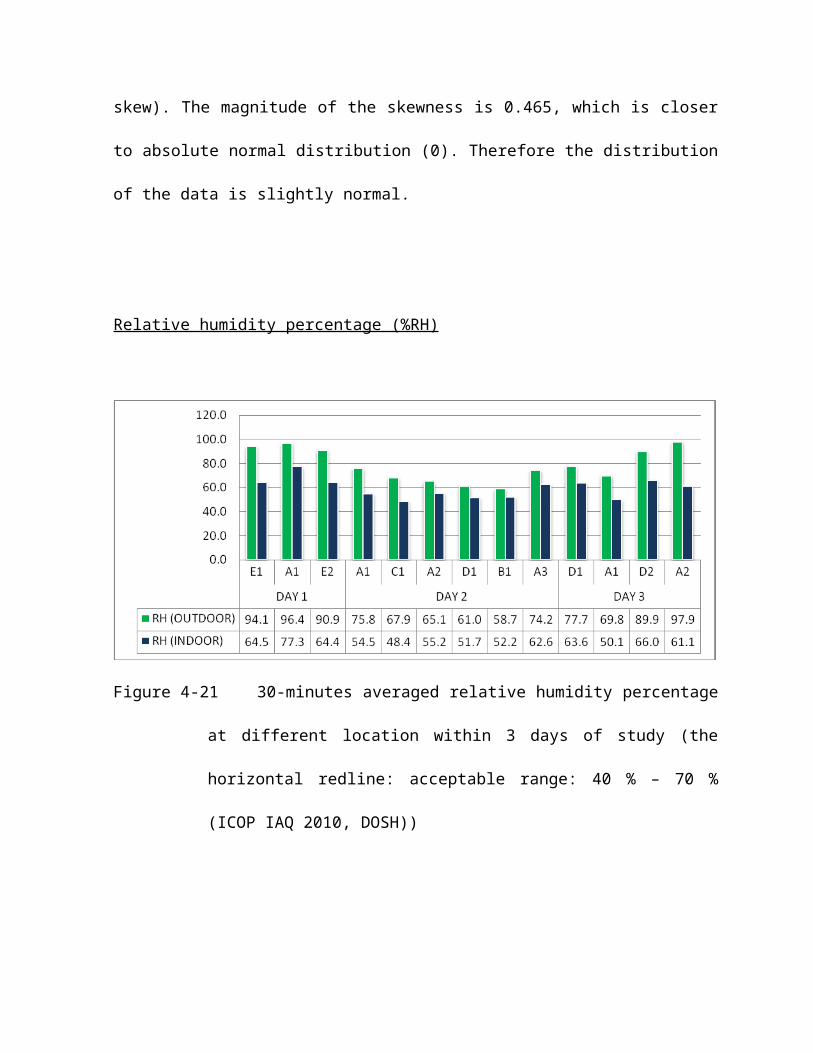
Industry Code of Practice Indoor Air Quality 2010, Department of Occupational Safety
& Health Malaysia. From the calculated TWA8hrs it is found that:
(1) None of the respirable particulates (PM10) is found to be exceeded 0.15
mg/m3 acceptable limit, based on TWA8hrs.
(2) The value of total volatile organic compound is exceeds the acceptable limit
of 3.0 ppm on December 4, 2014 (3.160 ppm) and nearly exceed the limit
on December 7, 2014 (2.928 ppm). However based on TWA8hrs none of the
TVOC concentration exceeds the limit.
(3) None of the carbon dioxide (CO2) level exceed acceptable limit of C1000
ppm, based on TWA8hrs.
(4) None of the ozone (O3) level exceed acceptable limit of 0.05 ppm, based on
TWA8hrs.
(5) None of the carbon monoxide (CO) level exceeds the acceptable limit of 10
ppm, based on TWA8hrs.
(6) Only temperature in December 4, 2014 (22.8 ⁰C) is less than acceptable
range of 23 – 26 ⁰C.
(7) None of the relative humidity found to be exceeded or less than acceptable
range of 40 – 70%.
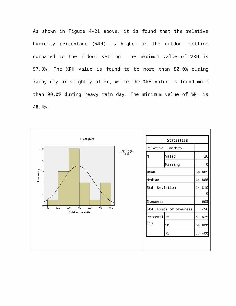
(8) Air speeds in all three days of study (December 4, 2014 (0.02 m/s);
December 5, 2014 (0.07 m/s); and December 7, 2014 (0.02 m/s) are less
than acceptable range of 0.15 – 0.50 m/s.
CHAPTER SIX
RECOMMENDATION AND CONCLUSION
Regarding the vehicle
It is suggested a massive campaigns need to be done from the national level to the
bottom strata to encourage fleet industries to shift into cleaner fuel substances in
vehicle power generation, such as by using low-sulphur content diesel, as well as to
use appropriate device, such as the use of three-way (oxidation-reduced) catalytic
converter to reduce the pollution emission (Faiz, A et al, 1996; Bailey & Solomon,
2004; WHO)
Heavy vehicle is suggested to be licensing and the renewal must be done annually.
Prior to the new license issued, a regular monitoring and maintenance in ensure
cleaner emission needs to be conducted. Unlicensed heavy duty vehicle needs to be
banned from the road (WHO).
The government of Singapore has already amended a new smoke emission limit for
vehicle fuelled with diesel entering the country from Malaysia, from 50 HSU to 40
HSU effectively July 1, 2014. This is a serious approach at the national level, which
can be followed by Malaysia Government. To ensure the HSU level below the
acceptable limit, several recommendations has been published by Department of
Environment Malaysia to all vehicle owner: (1) adhere to recommended maintenance
schedule; (2) undergo periodic smoke inspection; (3) service the fuel injector as well
as the fuel pump for every 20,000 km mileage; and (4) overhauled engines every
100,000 km mileage (DOE Malaysia, 2014).
Last but not least, as suggested by Bailey D and Solomon G, there is a need to
regulate the requirement for the driver to reduce speed once approaching near the
inspection bay and offices as well as switching off the engine while parked in the
inspection bay or any other area around, regardless the duration the vehicle stopping
in the parking area.
Regarding the building
According to Maroni (1998), the proper design and construction of building is
important strategy to gain better indoor air quality. As the building is already existed,
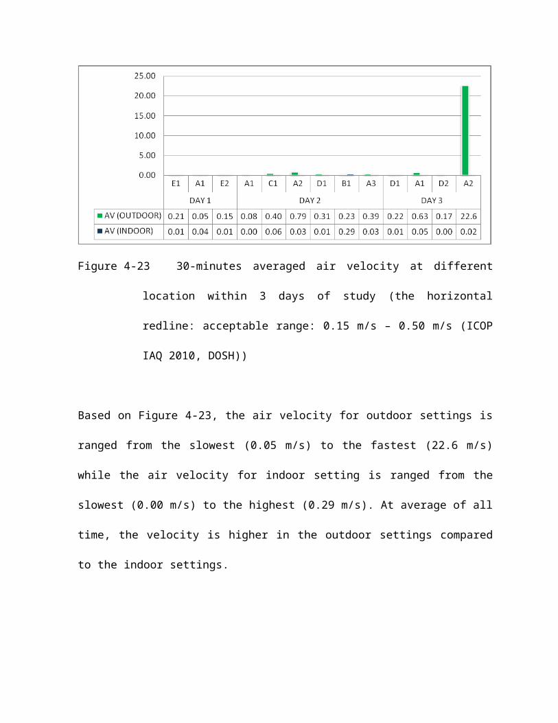
the second strategy needs to be implemented appropriately. The first step is to
control the source. As the source in Import Lane is coming from the outdoor
environment, the penetration and the infiltration of the pollutants need to be
minimized as far as practicable. Door and windows need to be kept close at all time
an only opened during entering or exiting the room. Cracks and fractures on the wall
need to be plastered. As the offices in Import Lane, KSAB use fresh air via Water
Cooling Package Unit (WPCU), it is important to shield the fresh air intake with
appropriate and adequate air pollution air pollution filter or absorbent.
Secondly, there are requirement to keep the indoor air well ventilated. Well ventilated
condition means a good air change, where there is input from the fresh air, circulating
the indoor setting and then exhausted the contaminated air to the outside. The best
way to maintain well ventilation is by opening the door and windows, which seems to
be contrast with the above statement regarding pollution source elimination, in case
of Import Lane, KSAB. Therefore, an engineering approach is used, with the
installation of air curtain. According to Paul and Tiwari (2014), air curtain which is
mounted on the of the doorway not only play a role as insect shield, but also can
prevent outdoor air infiltration, thus avoiding dust and air pollutants from entering the
indoor settings. This energy efficient technology helps in achieving a better indoor
comfort, thus supplying indoor fresh air for well and adequate ventilation.
The third approach in Maroni’s second strategies is to clean the air. There are
varieties of air cleaners in the markets, ranging from cheaper-table top instrument to
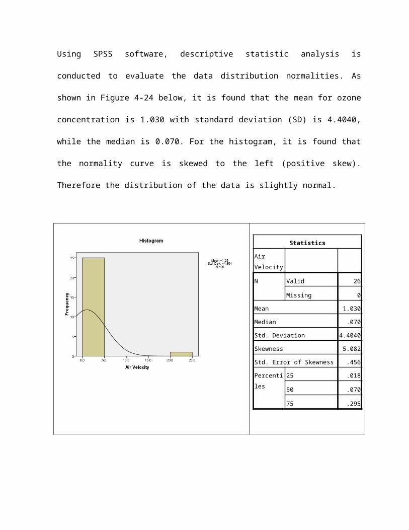
the expensive-whole floor coverage device. Most of the cleaners are only suitable in
wiping off particles in the air, but not the gases pollutants. Gases pollutant can only
be eliminated by diluting the concentration. One of the important indicator that
showing the air in one area is cleaned is through the absent of the dust on the ceiling
and wall surface as well as no webbing on the surfaces.
As for the last approach, controlling the exposure group, the occupant in the area
needs to located at the appropriate setting such as not under the exhaust sump or in
the contamination pathway of the room air, where this sump is design to collect all
contamination in the room air and returned it to the system. During this study, I have
noticed one RMC Officer in the office of Urusetia Kastam Import, Seksyen Jaminan
Bank, always keep tissues in her hand. From the interview done, I found that she has
been transferred to this Section in June 2014. Since then she experience sneezing,
eye and throat irritation and several other symptoms of Sick Building Syndrome. She
admitted since positioned in the section, she have taken days of medical leave due to
discomfort condition she experience. During visit to her desk, the DOSH Officer who’s
accompanied me during the first day of measurement, and I immediately found that
the table she’s position is in the pathway of contamination sump. A briefing has been
given to her and her colleague and suggesting her to adjust her position into the right
place.
Last but not least, regular monitoring is suggested to be conducted to ensure at all
time, the condition is not compromising the health status of the occupant.

Regarding the people
As the concentration of particulate matter in the indoor settings have no significant
difference with the outdoor particulate matter concentration, the officers from RMC as
well as OGA may face and breathing this contaminated air daily during working time.
Although wearing the personal protective equipment such as face mask may be
suitable during conducting the inspection in the bay, the best way to prevent adverse
effect is to implement the Maroni’s strategies in achieving good indoor air quality.
Conclusion
The study area, Inspection Bays and offices at Import Lane, KSAB, is a well known
and designated to be the pathway of all vehicles type which are involved in carrying
consignment (in this case, import consignments from Singapore into Malaysia). The
majority of the vehicles are heavy duty carriers or heavy weight carriers which of
them using diesel as fuel. From the monitoring results obtained, there are no
statistically significant differences in the particulate matters concentration between
the outdoor environments and in the indoor settings. The I/O ratio is vary from 0.748
for PM10, 0.754 (PM4), 0.766 (PM2.5) to 0.785 for PM1. The ratio is higher when the
diameter size of the particles is smaller. However, the difference of 20% is small
compared to the ability of the pollutants to travel, influenced by the air direction and
velocity. The concentration during peak hour usually in the evening up to quarter of
the night is found to be closer to the acceptable limit stipulate in relevant guideline.
The mitigation measures rely on the three components, regarding the vehicles as the
source of the pollution; regarding to the building; and regarding to the exposed group
itself. Regarding to the vehicles, the administrative approaches by regulating several
requirements may be the best to suit the elimination and isolation of the pollution
sources. Regarding the building and the exposed group, Maroni’s combination of
strategies may be the best to ensure well condition to promote good indoor air
quality. The use of air curtain, an engineering approach is strongly suggested to be
implemented to shield the outdoor pollutants from entering the indoor settings.
REFERENCES
Bailey, D. & Solomon, G. (n.d.). Pollution prevention at port: clearing the air. Environmental
Impact Assessment Review .
Brugge, D. et al. (2007). Near-highway pollutants in motor vehicle exhaust: A review of
epidemiologic evidence of cardiac and pulmonary health risks. Environmental Health
, 6 (23).
(2000). Chapter 7.3 Particulate Matter. In Air Quality Guidelines - Second Edition.
Copenhagen: WHO Regional Office for Europe.
Charron, A. & Harrison, R.M. (2005). Fine (PM2.5) and Coarse (PM2.5-10) Particulate Matter
on a heavily trafficked london highway: sources and processes. Environmental
Science Technology , 39 (20), 7768-7776.
Clark, N.N. et al. (1999). Field measurement of particulate matter emissions, carbon
monoxide, and exhaust opacity from heavy-duty diesel vehicles. Journal of the Air &
Waste Management Association , 49 (9), 76-84.
Colvile, R.N. et al. (2001). The transport sector as a source of air pollution. Atmospheric
Environment , 35 (9), 1537-1565.

Department of Environment Malaysia. (n.d.). Retrieved from Official Air Pollution Index of
Department of Environment: http://apims.doe.gov.my/apims/2012/index.php
Department of Environment Malaysia. (n.d.). Retrieved from New Smoke Emission Limit for
Diesel Vehicles Entering Singapore:
http://www.doe.gov.my/portalv1/en/info-umum/had-baru-pelepasan-asap-bagi-
kenderaan-diesel-yang-memasuki-singapura/314311
Department of Environment Malaysia. (n.d.). Retrieved from Air Quality:
http://www.doe.gov.my/portalv1/en/info-umum/kuality-udara/114
Department of Environment Malaysia. (n.d.). Retrieved from Indoor Air Quality:
http://www.doe.gov.my/portalv1/en/info-umum/english-indoor-air-quality/125
Estokova, A. & Stevulova, N. (2012). Investigation of suspended and settled particulate
matter in indoor air. InTech , 455-480.
Fairus M-D. et-al. (2011). Preliminary Assessment of Indoor Air Quality in Terrace Houses.
Health and the Environment Journal , 2 (2), 8-14.
Faiz, A et al. (1996). United Nations. Retrieved from Air Pollution from Motor Vehicles:
Standards and Technologies for Controlling Emissions:
http://www.un.org/esa/gite/iandm/faizpaper.pdf
Garshick, E et al. (2008). Lung Cancer and Vehicle Exhaust in Trucking Industry Worker.
Environmental Health Perspective , 116 (10), 1327-1332.
Garshick, E. et-al. (2012). Lung cancer and elemental carbon exposure in trucking industry
workers. Environmental Health Perspectives , 120 (9), 1301-1306.
Gillies, J.A. et al. (2001). On-road particulate matter (PM2.5 and PM10) emissions in the
Sepulveda Tunnel, Los Angeles, carlifornia. Environmental Science Technology , 35
(6), 1054-1063.
Grau-Bove, J. & Strlic, M. (2013). Fine particulate matter in indoor cultural heritage: a
literature review. Heritage Science , 1 (8).
GrayWolf Sensing Solutions. (n.d.). Retrieved from AdvancedSense DirectSense IAQ:
http://www.wolfsense.com/pdf/GrayWolf-Indoor-Air-Quality-IAQ-Meter-Brochure-
lo.pdf
GrayWolf Sensing Solutions. (n.d.). Retrieved from DirectSenseAir Air Velocity Meters:
http://www.wolfsense.com/air-velocity-meter.html
Industry Code of Practice on Indoor Air Quality 2010. (2010). Putrajaya: Department of
Occupational Safety & Health Malaysia.
Janssen, N.A.H. et al. (2001). Assessment of exposure to traffic related air pollution of
children attending schools near motorways. Atmospheric Environment , 35 (22),
3875-3884.
Jones, A.M. & Harrison, R.M. (2006). Estimation of emission factors of particle number and
mass fractions from traffic at a site where mean vehicle speeds vary over short
distances. Atmospheric Environment , 40 (37), 7125-7137.
Kaur, S. et al. (2007). Fine particulate matter and carbon monoxide exposure concentrations
in urban street transport microenvironments. Atmospheric Environment , 41 (23),
4781-4810.
Maroni, M. (1998). Health Effects on Indoor Air Pollutants and their Mitigation and Control.
Radiation Protection Dosimetry , 78 (1), 27-32.
Marr, L.C. et al. (2004). Vehicle traffic as a source of particulate polycyclic aromatic
hydrocarbon exposure in the Mexico City metropolitan area. Environmental Science
Technology , 38 (9), 2584-2592.
McCreddin, A. et al. (2013). Personal Exposure to Air Pollution in Office Workers in Ireland:
Measurement, Analysis and Implication. Toxics , 1, 60-76.
Michael J. Kleeman, et-al. (2000). Size and Composition Distribution of Fine Particulate
Matter Emitted from Motor Vehicles. Environmental Science & Technology , 24 (7),
1132-1142.
Ministry of Environmental Protection (MEP), National Development Reform Commission
(NDRC) & ministry of Finance, China. (2013). "Twelfth five-year plan" on air pollution
prevention and control in key regions (English translation). China: Clean Air Alliance
of China.
Ministry of Health Malaysia. (2013, July). Retrieved from Health Fact 2013:
http://www.moh.gov.my/images/gallery/publications/HEALTH%20FACTS
%202013.pdf
Moller, K.L. et al. (2014). Occupational exposure to ultrafine particles among airport
employees - combining personal monitoring and global positioning system. PLOS
ONE , 9 (9).
Muhamad A. et-al. (2000). Air quality in Malaysia: Impacts, management issues and future
challenges. Respirology , 5 (2), 183-196.
N.B.A. Wahid et-al. (2014). Source identification of particulate matter in a semi-urban area of
Malaysia using multivariate techniques. Bulletin Environmental Contamination
Toxicology , 92, 317-322.
Naeher, L.P. et al. (2000). Particulate Matter and Carbon Monoxide in Highland Guatemala:
Indoor and Outdoor Levels from Traditional and Improved Wood Stoves and Gas
Stoves. Indoor Air , 10, 200-205.
Norela S. et-al. (2005). Concentration and Composition Of PM10 in Outdoor and Indoor Air
in. Sains Malaysiana , 34 (2), 43-47.
Nur Zafirah M.S. & Marzuki I. (2011). Indoor and Outdoor Relationships of Respirable
Suspended Particulate Matter at Primary Schools in Kuala Terengganu, Malaysia.
Indoor and Built Environment .
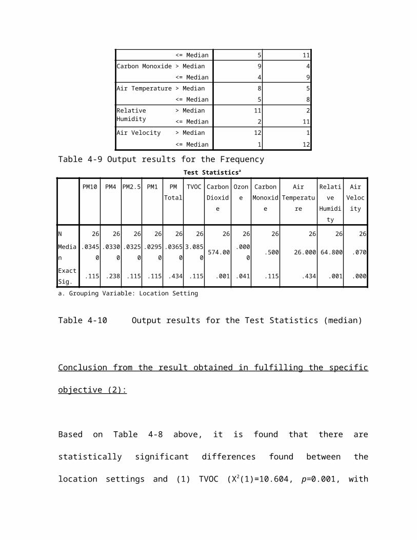
Paul, A. & Tiwari, A.C. (2014). Performance Analysis of Air Curtain: A Review of CFD
Approach. Corona Journal of Science and Technology , 3 (1), 1-7.
S.C. Lee & M. Chang. (2000). Indoor and outdoor air quality investigation at schools in Hong
Kong. Chemosphere , 41 (1-2), 109-113.
San Joaquin Valley Air Pollution Control District. (n.d.). Retrieved from Particulate Matter
(PM) Sources:
http://www.valleyair.org/Air_Quality_Plans/AQ_plans_PM_sources.htm
Sheesley, R.J. et al. (2008). Assessment of diesel particulate matter exposure in the
workplace: freight terminal. Journal Environmental Monitoring , 10, 305-314.
Thorpe, A. & Harrison, R.M. (2008). Sources and properties of non-exhaust particulate matter
from road traffic: a review. Science of the Total Environment , 400 (1-3), 270-282.
U.S. Environmental Protection Agency. (n.d.). Retrieved from Air Quality Management Online
Portal: http://www.epa.gov/airquality/aqmportal/management/monitoring.htm
U.S. Environmental Protection Agency. (n.d.). Retrieved from Quality Assurance Handbook
for Air Pollution Measurement System Volume II Ambient Air Quality Monitoring
Program: http://www.epa.gov/ttnamti1/files/ambient/pm25/qa/QA-Handbook-Vol-
II.pdf
Wahlina, P. et al. (2001). Experiment studies of ultrafine particles in streets and the
relationship to traffic. Atmospheric Environment , 35 (Supp. 1), S63-S69.
Weijers, E.P. et al. (2004). Variability of particulate matter concentrations along road and
motorways determined by a moving measurement unit. Atmospheric Environment ,
38 (19), 2993-3002.
WHO Regional Office of Europe. (2000). Retrieved from The Right to Healthy Indoor Air:
http://www.euro.who.int/__data/assets/pdf_file/0019/117316/E69828.pdf
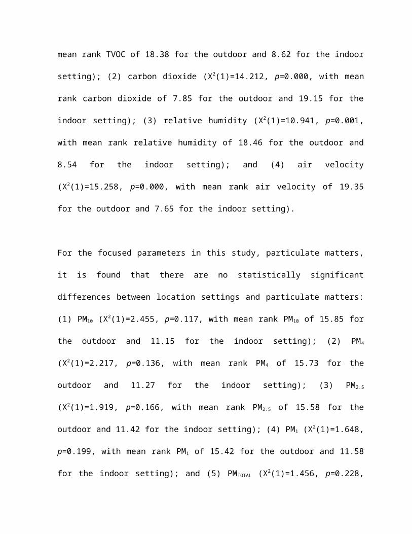
World Health Organization. (n.d.). Retrieved from Ambient (outdoor) air quality and health:
http://www.who.int/mediacentre/factsheets/fs313/en/
Xianglu Han, Luke P. Naeher. (2006). A review of traffic-related air pollution exposure
assessment studies in the developing world. Environment International , 32 (1), 106-
120.
Yu-Hsiang, C. et al. (2012). Temporal variations in airborne particulate matter levels at an
indoor bus terminal and exposure implications for terminal workers. Aerosol and Air
Quality Research , 12, 30-38.
Zhang, J. & Smith, K.R. (2003). Indoor air pollution: a global health concern. British Medical
Bulletin , 68, 209-225.
Zhu, Y. et al. (2002). Study of ultrafine particles near a major highway with heavy-duty diesel
traffic.