NBER WORKING PAPER SERIES

INTERTEMPORAL CONSTRAINTS, SHADOWPRICES, AND FINANCIAL ASSET VALUES

Robert S. Chirinko

Working Paper No. 2247

NATIONAL BUREAU OF ECONOMIC RESEARCH1050 Massachusetts Avenue

Cambridge, MA 02138May 1987

The author wishes to thank Alan Auerbach, David Bradford, Donald Cox, Fumio Hayashi,and Lars Muus for their helpful comments and to acknowledge financial support fromthe National Science Foudation under Grant No. SES-8309O73. All errors, omissions,and conclusions remain the sole responsibility of the author. The research reportedhere is part of the NBER's research program in Economic Fluctuations. Any opinionsexpressed are those of the author and not those of the National Bureau of EconomicResearch.

NBER Working Paper #2247May 1987

Intertemporal Constraints, Shadow Prices, and Financial Asset Values

ABSTRACT

The conditions under which the unobserved shadow price of

capital can be equated to the financial value of the firm have been

developed in an important paper by Hayashi (1982). Employing a more

powerful analytic method, this paper reexamines the shadow price-asset value relation in a model with a general set of intertemporal

constraints. For a model with one capital good, a general relation

between shadow prices and asset values is derived, and restrictive

assumptions implicit in previous work are highlighted. Of particularimportance is the relation between the marginal and average survival

rates of capital, and the critical role of geometric depreciation. The

impact of a discrete-time framework in specifying and interpreting

econometric models is also explored.

Robert S. ChirinkoCommittee on Public

Policy StudiesUniversity of Chicago1050 East 59th StreetChicago, IL 60637

INTERTEMPORAL CONSTRAINTS, SHADOW PRICES. AND

FINANCJAL ASSET VALUES

I. Introduction

In dynamic models of the firm, intertemporal constraints are

represented by distributed lag and convex technologies. In the

presence of the former constraint (e.g., capital accumulation), shadow

prices play the critical role in intertemporal allocation decisions, but

are not generally observed by applied econometricians. This

problem is likely to occur when the model also includes convex

constraints (e.g., adjustment costs), and has been addressed in one of

two ways. The first solution specifies and estimates the underlying

stochastic process for the components of the unobservable, and then

computes the shadow price from forecasts of its components. This

class of solutions includes the two-step procedure of Abel and

Blanchard (1984), the maximum likelihood estimator of Hansen and

Sargent (1980), and the Euler equation technique of Hansen and

Singleton (1982); in the latter case, the forecasting equations are

determined by the choice of instruments. These methods arose in

response to the critique of Lucas (1976), who argued that "any

change in policy will systematically alter the stmcture of

econometric models" (p. 41). Under this view, changes in policy are

identified as changes in the parameters governing policy outcomes,

and these parameters will generally affect forecasts of economic

variables. Only if one maintains that the sample period contains no

changes in policy or non-policy factors affecting the positedstochastic process will the forecasting solution to the unobserved

shadow price problem be valid.

2

The second class of solutions, which will be the focus of this

paper, relates financial asset values to the unobserved shadow

prices, and possesses the substantial advantage that estimation can

proceed even in an unstable stochastic environment. In an

important paper, Hayashi (1982) developed the conditions underwhich the shadow price of capital could be equated to the value of

the firm as assessed on asset markets, thus providing a formal

theoretical foundation for the Tobin's (1969) Q model of investment.1

Limited by the analytic method, however, this work did not

recognize the significance of a number of implicit assumptions

concerning distributed lag constraints. Employing the techniques

introduced by Kamien and Muller (1976), the current study will be

able to highlight the importance of these distributed lag constraints

on the shadow price-asset value relation.

A general discrete-time model of the firm with one capital good

but two distributed lags is developed and analyzed in Section II. The

relation between shadow prices and asset values are drawn in

Section III and, when restrictive assumptions concerning the

distributed lag technology are relaxed, the usefulness of asset price

data is severely compromised. The conditions under which asset

prices remain useful to the applied econometrician and the impact of

a discrete-time framework on the specification and interpretation of

econometric models are also explored.

1 See Chirinko (1987) for a survey of Q models utilized in the studyof business fixed investment. Hasbrouck (1985) has used Q to studytakeovers; Lindenberg and Ross (1981), Salinger (1984), andSmirlock, Gilligan and Marshall (1984) to examine the relationshipbetween firm rents and market structure

II. Conditions Characterizing An Optimum

In this section, a general model of the firm containing both

distributed lag and convex constraints is developed. The firm

chooses labor inputs and one capital input to maximize its end ofperiod equity value (V0), defined as the discounted sum of net

revenues (7t[Kt1}),

= t: 01,t r[Kt.i], (la)

01,t = sUi (l+p)-1, (ib)

where t[.] is defined with respect to the optimal level of the variable

labor inputs, 01, is the discount factor between periods 1 and t, and

Ps is the one-period discount rate. Net revenues depend positively

on the capital stock available at the beginning of the current period

(K..i; i.e., at the end of the previous period), and become available to

the firm at the end of the current period. For notational convenience,

all relative prices are assumed constant, and taxes are omitted.

The firm can increase its capital stock only indirectly through

the placement of new orders (Or) and, in maximizing (1), faces two

distributed lag constraints.2 First, the quantity of delivered capital

goods (Dr) is determined through the delivery lag by current and

past orders. Second, following delivery, capital depreciates overtime, and the capital stock depends on a fixed set of survival weights.

2 The model can be expanded easily to include additional distributedlag constraints - for example, the gestation lag between deliveriesand increments to the productive capital stock and the expenditurelag between orders and payments.

3

4

These two constraints are represented by the following linear

technologies ,3

D = It-s Os, 0 � � 1 u=O,b (2a)

K = D5, 0 � � 1 u=0,d (2b)t—d

where b is the length of the delivery lag, d is the length of capital's

useful life, and the 13's and 6's represent the delivery and capital

depreciation technologies, respectively. In this discrete-time

framework, deliveries and net revenues (including expenditures) are

received and the capital stock is altered at the end of the period.

Current deliveries thus have no effect on current net revenues, and

do not begin depreciating until the following period (i.e., ö=1).

In addition to the distributed lag constraints (2), the firm faces

two convex constraints representing the adjustment costs associated

with placing orders and incorporating new capital into the production

process.4 These costs are represented in the model as negative

arguments in the net revenue function.

In calculating the necessary conditions for an optimum, we

could substitute for D and K..i with (2) and then differentiate (1)

with respect to new orders. Even with relatively simple technologies,

the resulting computations can prove complex, and economic

interpretations can be obscure. A preferred alternative, introduced

3 In general, these technologies may depend on the control and statevariables or on time. Consideration of these more generalrepresentations usually leads to models that are empiricallyintractable, and would thus obfuscate the main results in this paper.4 Adjustment costs were analyzed initially in the models of Eisnerand Strotz (1963) and Lucas (1967), and are an intergal element inthe Tobin's Q investment model (Abel, 1979; Hayashi, 1982).

by Kamien and Muller (1976), is to append the constraints to (1)with multipliers 4 and X, and form the Lagrangian,

£ = 1e1,t{7t[Kt.1,Ot,Dt] - -

+ t1°' s1 S

(3)91,t A D5

+ 01,t { Do, + X Ko,}.

The sums for the delivery and depreciation lags have been split into

two parts to separate variables that depend on current decisions and

those that are predetermined (though not necessarily constant) from

the beginning of period 1 onward. These predetermined variables

are defined as follows,

Do, = Os, 0 � t � b (4a)

Ko, = D5. 0 � t � d (4b)

Since Do,t and Ko, represent precommittments made prior to period

1, they will not affect optimal choices over the planning horizon, but

will be important in linking the financial value of the firm to the

shadow price of capital.

5

6

To facilitate the calculation of the necessary conditions for an

optimum, it will prove convenient to utilize the following

transformation,5t t+c

?-5 X = Oi, X (Ot,s/Ot,t) 'v , (5)t=1 s=1 t=1 s=t

where = {-S 6t-s}'

c = {b,d},X = {O,D},Vt = {4t,?t}.

With (3) and (5), we construct the following current-value

Hamiltonian,

H[Kt, D, O A., 4, t] =

ei, { D, Ot] - t - t K

t+b+ Ot (Ot,s/Ot,t) 13s-t 4s (6)s=t

.-

+ D (Ot,s/Ot,t) 8s-t 's } . t � 1

The necessary conditions for an optimum are computed by differ-

entiating H [.1 with respect to the state (Ks, D) and control (Or)

variables,6

5 The transformation follows directly by stating (5) in matrixnotation and then transposing the scalar expression.6 The necessity of these conditions for an optimum has beenestablished by Kleindorfer, Kleindorfer, and Thompson (1977) andWeitzman and Schmidt (1971).

7

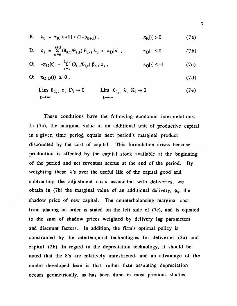
K: 7 = K[u+l] / (i+Pu+i), (7a)

= (6/9) + [s] D[I � 0 (7b)

0: -7r0[t} = b (Ot,s16t,t) 1- (7c)

0: 7t0,0(t) � 0, (7d)

Lim 01,t 4 D—O Lim 0,t ? K--*0 (7e)t—oo t—°°

These conditions have the following economic interpretations.

In (7a), the marginal value of an additional unit of productive capital

in a given time period equals next period's marginal productdiscounted by the cost of capital. This formulation arises because

production is affected by the capital stock available at the beginning

of the period and net revenues accrue at the end of the period. By

weighting these ?'s over the useful life of the capital good and

subtracting the adjustment costs associated with deliveries, weobtain in (7b) the marginal value of an additional delivery, 4, the

shadow price of new capital. The counterbalancing marginal cost

from placing an order is stated on the left side of (7c), and is equated

to the sum of shadow prices weighted by delivery lag parametersand discount factors. In addition, the firm's optimal policy is

constrained by the intertemporal technologies for deliveries (2a) and

capital (2b). In regard to the depreciation technology, it should be

noted that the 8's are relatively unrestricted, and an advantage of the

model developed here is that, rather than assuming depreciation

occurs geometrically, as has been done in most previous studies,

alternative patterns, such as straight-line or "one-hoss-shay," can be

considered. Throughout we assume that the constraints are always

binding and the optimal level of orders is always non-negative.

Since the constraints are linear, the Kuhn-Tucker constraint

qualifications are satisfied, and the sufficiency of (7) depends on the

properties of [.]

8

9

III. The Unobserved Shadow Price Of Capital And The Financial

Value Of The Firm

The above characterization of the firm's optimal policy is not

useful in empirical work because it contains variables unobserved by

the applied researcher.7 In the present context, this problem arisesbecause 4, depends on the path of ?'s extending far into the future.

In Proposition I, we explore the relation between the unobserved

shadow price of capital and the financial value of the firm in a

discrete-time framework with two distributed lag constraints.

Proposition I

V0 = t]O1t {4 D0, + Xt Ko,} m = max[b,d] (8)

if and only if

it[•] is homogeneous of degree one in all arguments and the output

and factor markets are perfectly competitive.

Derivation

The homogeneity of ic[] implies that

01,t { it[t] - 7r0[t] Ot - 7tD[t] D - °t+1,t+1 7tK[t+fl K } = 0. (9a)

7 While the firm has been endowed heretofore with perfect foresight,the model can be recast with no loss in generality as one in which thefirm maximizes expected profits, where expectations are conditionedon information known when decisions are being undertaken.

10

Sum over t from 1 to oe and substitute (7a), (7b), and (7c),

t+bei, { ir[t] + (Ot,s/Ot,t)

- 4 D (9b)

+ D: (Ot,s/Ot,t) 6.t X - ?. K } = 0.

The two inner sum in (9b) can be transformed according to (5),

10i,t[t1 = 10it { 4 [D O] (9c)

+ ? {K -si D] }.

In (9c), the left side is the value of the firm (la). On the right side,

the first term in braces represents deliveries from orders made priorto the beginning of the planning period (Doe; 4a); a similar

interpretation applies to the second braced term in regard to capital(K0,; 4b). Noting that Do, and Ko, are zero for t � m = max[b,d], we

obtain (8). The converse follows directly. II

In (9), the asset value of the firm does not identify the shadow

price of capital, as V0 depends on discount factors, shadow prices,

deliveries, and capital stocks extending m periods into the future.

The intuition underlying this result is that, since markets are

competitive, the firm is unable to earn any economic profits from

period 1 onward. The cash flows on the precommitted stocks

represent quasi-rents that are measured as the product of

anticipated deliveries and existing capital multiplied by their shadow

11

prices. The importance of the constant returns to scale assumption is

that these shadow prices are independent of the stocks.8

That the asset value of the firm is not a sufficient statistic for

identifying the shadow price of capital stems from two independent

factors. The first is that the financial markets generate only one

variable to evaluate the firm's profit possibilities, but these are

affected by the two state variables following from the distributed lag

constraints Multiple distributed lags arise when production depends

on multiple capital stocks with different technologies (Chirinko, 1982;

Wildasin, 1984) or, as highlighted in this model, when there is only

one capital stock but other constraints impinge on the firm.

However, the inadequacy of asset values extends beyond the number

of distributed lags, and also involves the nature of the distributed lag

parameters. If we assume that capital is delivered immediately

upon order (i.e., ij=l, 3=O, u=l,b), Do, = 0, and we obtain the

following relation,

Vo = t1 Ko, . (10)

In the case of only one distributed lag but with unrestricted

parameters, (10) indicates that the asset value remains unable to

identify the shadow price of capital. This important result is masked

when the analysis is conducted in terms of standard capital

transition equations that depend on geometric depreciation.The above considerations lead to the following proposition.

8 If relative prices were allowed to vary, then the assumption ofperfectly competitive markets would be needed to ensure theirindependence from current decisions.

12

Proposition II

Given the assumptions in Proposition I and the absence of a delivery

lag, the financial value of the firm and the shadow price of capital

are related as follows,

V0 = (4 (1—6) Ktj) / (l+pi) (11)

if and only if

capital depreciates according to a geometric pattern.

Derivation

Rewrite (10) as,d

V0 = o 9i,t 't 't (12a)

K0 = 6(-s) D, (12b)

= Ko,/Ko. (12c)

Note that b is the percentage of the capital stock from the

beginning of the planning period surviving in period t (i.e., the

average survival rate) and, in general, depends on the history of

delivered capital. Consider the following functional equation,

= (12d)

and its relation to the A's in (12a) and the 6's in (7b),

s0 s=O s=0 s0At = td D / td D = 6ttd D 'td = (1 2e)

Equation (12d) is Cauchy's functional equation of the exponential

function, and all non-trivial solutions to (12d) imply that the 's

follow a geometric pattern (Eichhom, 1978, Chapter l.4),9

st-s = (l6)ts = (l)t (l&)s = &t&s and d—oo. (12f)

Equation (12a) can be written as follows,

V0 = K 10i (l_o)t . (12g)

By (7b) with ltD[•] = 0 and (ib), we obtain (11). The converse follows

directly. li

The key condition underlying the derivation of Proposition II is that

the average survival weights for existing capital (At) equal themarginal survival weights for new capital (o), which are

independent of past acquisitions.10 Equation (11) states that thevalue of the firm at the beginning of the period equals the available

capital stock multiplied by the marginal gross return per unit ofcapital adjusted for depreciation.11 Since returns become available

9 The two trivial solutions are =O Vt,s, which is of no economicinterest, and =1 and 3=O Vt,s which defines a non-durablefactor of production.10 The relation between geometric depreciation and the constancy ofthe average replacement rate has been noted by Jorgenson (1974).11 This adjustment is needed because existing capital depreciatesimmediately while new capital begins depreciating the followingperiod. Since 4 is the shadow price for new capital, it must beadjusted for one period of depreciation.

13

14

at the end of the period, they are discounted by (1 +p 1).12

These adjustments for depreciation and discounting go

unnoticed in continuous-time models, and may have a measurable

effect on estimated investment models of the Tobin's Q variety. In

this class of models, 4 is the key regressor, and has been equated in

previous studies to Tobin's Q, defined as "the ratio of the market

value of existing capital to its replacement cost" (Hayashi, 1982, p.

214, italics in the original):

= Qcvl = / K1 , (13a)

This conventional specification of Q differs from the modified defini-

tion following from the discrete-time framework (Proposition H13

= Qmod = ((l+pt) -i) / ((1-6) K..i) , (13b)

12 Note that the presence of (1-6) and (i+pi) in (11) is independent ofthe assumption that only capital available at the beginning of theperiod affects current production. This timing convention is reflectedsolely in the definitions of 7t[.} (la) and (7a). If current deliverieswere permitted to affect current production through the capitalstock, then =13 Differences between the conventional and modified definitions ofQ would disappear if we maintained the unreasonable assumptionthat the firm receives its cash flows at the beginning of the periodand the more palatable assumption that new capital beginsdepreciating immediately upon delivery. In this model, the lattertiming assumption does not comport well with the exclusion ofcurrent deliveries from affecting current production (cf., (la) and(2b)).

and has two implications for the estimated coefficient on 4. First,this coefficient is usually interpreted as depending solely on the

adjustment cost technology.14 Equation (13b) reveals, however, thatit is properly interpreted as a combination of adjustment cost and

depreciation parameters. Furthermore, econometric Q models have

uniformly generated estimates of the 4 coefficient that imply

unreasonably sluggish responses of investment to variations in the

economic environment.'5 One explanation for this unsatisfactory

result is that QCV1 is excessively volatile relative to the time series for

investment. However, insofar as the firm's discount rate and

financial market value are negatively correlated, Qmod will be less

volatile, and may lead to more reasonably estimated parameters.

14 See Hayashi (1982, p. 218) or equation (7c) with separabilitybetween the adjustment cost and production technologies.15 See the simulations in Summers (1981) in which "only three-fourths of the ultimate adjustment of the capital stock takes placewithin twenty years" (p. 101).

15

16

IV. SUMMARY AND CONCLUSION

This paper has highlighted the importance of distributed lag

constraints on the shadow price-asset value relation. In a model

with only one capital good, there nonetheless exists a number of

distributed lag constraints that lead to additional state variables

impairing the usefulness of asset values in empirical work

(Proposition I). Even when the model was reduced to one state

variable, the unrestricted nature of the distributed lag parameters

precluded the firm's financial value from identifying the unobserved

shadow price of capital. In order for asset prices to regain their role

in empirical work, it was required that the survival weights on

capital follow a geometric pattern (Proposition II). With the implicit

assumptions concerning distributed lags made clear, these results

indicate to the applied researcher the conditions under which the

substantial information contained in asset prices can be exploited. If

delivery, expenditure, or gestation lags are viewed as important to

the problem under study, then asset prices will not prove useful in

estimation, and other methods of solving the unobservable

expectations problem will have to be utilized.16 However, these

distributed lags will be of less importance at lower frequencies and,

thus, the estimation of Q investment models is most likely to be

successful when conducted with annual data.

16 Empirical studies that incorporate these distributed lags and arebased explicitly on an optimizing framework are rare. See Chirinko(1987, Table II) for a review of the intertemporal constraints used inprevious investment studies, and Chirinko (1984) for a modelestimating distributed lag parameters with a two-step forecastingmethod.

17

REFERENCES

Abel, Andrew B., 1979, Investment and the Value of Capital (GarlandPublishing, New York).

_______ and Olivier Blanchard, 1984, "The Present Value ofProfits and Cyclical Movements in Investment," HarvardUniversity.

Chirinko, Robert S., 1982, "The Not-So-Conventional Wisdom Concern-ing Taxes, Inflation, and Capital Formation," National TaxAssociation - Tax Institute of America Proceedings, 272-281.

________ 1984, "New Orders and Lags in the Acquisition of Capital,"Hoover Institution, Stanford University.

_______ 1987, "Will 'The' Neoclassical Theory of Investment PleaseRise?: The General Structure Of Investment Models And TheirImplications For Tax Policy," in: Jack M. Mintz and Douglas D.Purvis, eds., The Impact of Taxation On Business Investment(John Deutsch Institute of Economic Policy, Kingston, Ontario).

Eichhorn, Wolfgang, 1978, Functional Equations in Economics(Addison-Wesley, Reading, Massachusetts).

Eisner, Robert, and Robert H. Strotz, 1963, "Determinants of BusinessInvestment," in: Commission On Money And Credit. Impacts OfMonetary Policy (Prentice-Hall, Englewood Cliffs, New Jersey).

Hansen, Lars P., and Thomas J. Sargent, 1980, "Formulating andEstimating Dynamic Linear Rational Expectations Models,"Journal of Economic Dynamics And Control 2, 9-46.

_______ and Kenneth J. Singleton, 1982, "Generalized InstrumentalVariables Estimation Of Nonlinear Rational ExpectationsModels," Econometrica 50, 1269-1286.

Hasbrouck, Joel, 1985, "The Characteristics of Takeover Targets:q and Other Measures," Journal of Banking and Finance 9,351-3 62.

Hayashi, Fumio, 1982, "Tobin's Marginal q and Average q: ANeoclassical Interpretation," Econometric a 50, 213-224.

Jorgenson, Dale W., 1974, "The Economic Theory of Replacement andDepreciation," in: Willy Sellekaerts, ed., Econometrics andEconomic Theory Essays in Honour of Jan Tinbergen(International Arts and Sciences Press, White Plains, NewYork), 189-221.

Kamien, Morton I., and E. Muller, 1976, "Optimal Control WithIntegral State Equations," The Review Of Economic Studies 43,469-47 3.

Kleindorfer, G.B., P.R. Kleindorfer, and R.L. Thompson, 1977, "TheDiscrete Time Maximum Principle," in: Charles Tapiero, ed.,Managerial Planning: An Optimum and A Stochastic ControlApproach (Gordon Breech Science Publishers, New York),375-3 82.

Lindenberg, Eric B., and Stephen A. Ross, 1981, "Tobin's q Ratio andIndustrial Organization," Journal of Business 54, 1-32.

Lucas, Robert E., 1967, "Optimal Investment Policy And The FlexibleAccelerator," International Economic Review 8, 78-85.

_______ 1976, "Econometric Policy Evaluation: A Critique," in: KarlBrunner and Allan H. Meltzer, eds., Carnegie-RochesterConferences in Public Policy, The Phillips Curve and LaborMarkets (North-Holland, Amsterdam), 19-46. Reprinted, 1981,in: Studies in Business Cycle Theory (MIT, Cambridge),104-130.

Salinger, Michael A., 1984, "Tobin's q, Unionization, and theConcentration-Profits Relationship," Rand Journal of Economics15, 159-170.

Smirlock, Michael, Thomas Gilligan, and William Marshall, 1984,"Tobin's q And The Structure-Performance Relationship,"American Economic Review 74, 1051-1060.

Summers, Lawrence H., 1981, "Taxation and Corporate Investment: Aq-Theory Approach," Brookings Papers on Economic Activity1981.1, 67-140.

18

Tobin, James, 1969, "A General Equilibrium Approach To MonetaryTheory," Journal of Money. Credit. And Banking 1, 15-29.

Weitzman, Martin L., and Schmidt, A.G., 1971, "The MaximumPrinciple for Discrete Economic Processes on an Infinite TimeInterval," Kibernetika 5, 22-35.

Wildasin, David E., 1984, "The q Theory Of Investment With ManyCapital Goods," American Economic Review 74, 203-210.

19