VIC Frozen Soils Simulation in Permafrost Regions: Modifications, Improvements, and Testing
44
Simulation in Permafrost Regions: Modifications, Improvements, and Testing Jennifer Adam Amanda Tan May 2, 2007 Hydro Group Seminar
description
VIC Frozen Soils Simulation in Permafrost Regions: Modifications, Improvements, and Testing. Jennifer Adam Amanda Tan May 2, 2007 Hydro Group Seminar. Talk Overview. Motivation Model Description Model Improvements Study Domain Testing of Model Improvements Conclusions. - PowerPoint PPT Presentation
Transcript of VIC Frozen Soils Simulation in Permafrost Regions: Modifications, Improvements, and Testing

VIC Frozen Soils Simulation in
Permafrost Regions Modifications
Improvements and Testing
Jennifer AdamAmanda Tan
May 2 2007
Hydro Group Seminar
Talk Overview1 Motivation 2 Model Description 3 Model Improvements 4 Study Domain 5 Testing of Model Improvements 6 Conclusions
Motivation
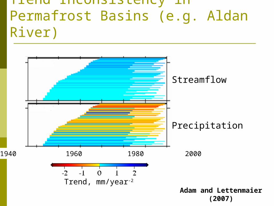
1 PrecipitationStreamflow Trend Inconsistency in Permafrost Basins (eg Aldan River)
1940 1960 1980 2000
Adam and Lettenmaier (2007)
Trend mmyear-2
Precipitation
Streamflow
Winter Summer Winter Summer
Permafrost Definition (loose)
Seasonally Frozen Ground Permafrost
Active Layer
Permafrost Layer cm km
cm m
2 Active Layer Depth Simulated Poorly
Snow cover extent lake freeze and break-up dates streamflow climatology ndash satisfactory
Permafrost active layer depth ndash unsatisfactory
Su et al (2005)
3 Historical Streamflow Trends Not Captured in Permafrost Basins
Observed
Simulated
Yenisei
LenaQ
103
m3 s
-1
1940 1960 1980 2000
Obrsquo
Q 1
03 m
3 s-1
1940 1960 1980
Permafrost BasinsNon-Permafrost Basin
Model Description
Frozen Soils Simulation Heat Equation
tL
zT
ztTC i
fis
(Cherkauer et al 1999) With parameterizations for Cs κ and θi
Term 1Heat
Storage(Time)
Term 2Vertical
Heat Conduction
(Space)
Term 3Latent Heat
(Time)
VIC Frozen Soils Algorithm Cherkauer and Lettenmaier
(1999) finite difference algorithm
solving of thermal fluxes through soil column
infiltrationrunoff response adjusted to account for effects of soil ice content
parameterization for spatial distribution of frost
tracks multiple freezethaw layers
can use either ldquozero fluxrdquo or ldquoconstant temperaturerdquo bottom boundary
(Cherkauer et al 1999)
Current Implementation
(Cherkauer et al 1999)
Spatial Frost Algorithm To produce a
spatial distribution of ice content and subsequently soil moisture drainage
(Cherkauer et al 2003)
Frozen Soils Optionshellip WOW NODES 18 number of soil thermal nodes FULL_ENERGY TRUE run full energy balance mode GRND_FLUX TRUE solve surface energy balance FROZEN_SOIL TRUE run frozen soils QUICK_FLUX FALSE Liang et al 1999 otherwise
Cherkauer et al 1999 QUICK_SOLVE FALSE Cherkauer et al 1999 for final
step only Liang et al 1999 for rest NOFLUX TRUE zero flux bottom boundary IMPLICIT TRUE uses implicit solver (NEW) EXP_TRANS TRUE exponential grid transform (NEW) QUICK_FS FALSE linear equations for max unfrozen
water content (not tested) QUICK_FS_TEMPS 7
SPATIAL_FROST TRUE sub-grid frost distribution FROST_SUBAREAS 10
Dp 15 damping depth (m) Tave -42 temp at damping depth (degC)
Changes and Improvements
1 Zero Flux Bottom Boundary Parameterization
2 Exponential Grid Transformation3 Implicit Solver4 Patch for the ldquoCold Noserdquo Problem
1 Soil Temperature Sensitivity to Bottom Boundary Specification
Soil
Tem
pera
ture
degC
1930 1931 1932 1930 1931 1932 1930 1931 1932
Constant T BBDp = 4 m
Tbinit = -12 degC10
0
-10
-20
Zero Flux BBDp = 4 m
Tbinit = -12 degC
Zero Flux BBDp = 15 m
Tbinit = -3 degC
Soil Surface (Top Boundary)Soil Bottom Boundary
BB Temperature Initialization
Annual Soil Temperature 32 m C
-6 -4 -2 0 2 4 6
A) Frauenfield et al 2004 station data
B) Interpolated station data
2 Exponential Grid Transformation
Linear Distribution
Exponential Distribution
bull Parameters Dp=15m Nnodes=18
z1=soil depth1
z2=2soil depth1
zi=linearly distributed to Dp
Problem discontinuity in
Δz between nodes 2 and 3
zi=exp(bi)+c
Problem discontinuity in Δz between all
nodes
1 m
3 m
5 m
7 m
9 m
11 m
13 m
15 m
i=0
i=Nnodes-1
Exponential Grid Transformation continuedbull Transform spatial derivatives only (temporal
derivatives are unaffected)
bull Expand heat conduction term (chain rule) because κ varies with z
2
2
zT
zT
zzT
z
tL
zT
ztTC i
fis
Exponential Grid Transformation continuedbull Introduce new space variable η (T will vary
exponentially with z but linearly with η)
bull Develop transform function η=f(z)
cbz )exp(
T
zzT
T
zT
zzT
2
2
2
2
2
2
zz
(chain rule)
)ln(1 czb
Exponential Grid Transformation continued Determine partial derivatives (in η)
Substitute partial derivatives with η into heat conduction terms
1)ln(1 cz
bz 2
2
2
)ln(1 cz
bz
2
2
zT
zT
z
z
Tczbz
Tczbz
Tzczb 22
2
22 )ln(1
)ln(1
)ln(1
new elements
Exponential Grid Transformation continued Determine constants b and c
Boundary condition 1 z(η=Nnodes-1) = Dp Boundary condition 2 z(η=0) = 0 Therefore c = -1
Solve in η-space (because the η-nodes are linearly distributed the finite difference assumptions are not compromised)
Map temperatures in η-space back to z-space Recalculate Cs κ and θi as a function of T for each
z-node
)1()1ln(
NnodesDpb
3 Implicit Solvers
Time
Spac
e
(The
rmal
Nod
es)
t-1 t
0123456
Explicit (forward in time)
Implicit (backward in time)
knownunknown
7 explicit equations solved independently
7 implicit equations solved simultaneously
Time
Spac
e
(The
rmal
Nod
es)
t-1 t
0123456
Stability Issues Stability of convergence
Implicit unconditionally stable Explicit satisfy the Courant-Friedrichs-Lewy Condition
λle14 for no oscillating errorsλ=16 to minimize truncation error
(solution make Δtle1hr or Δzge02m ) Ability to find a solution
Explicit not an issue with physically reasonable values (root_brent is very robust)
Implicit often is unable to find a solution at the initial formation of ice in the soil column
2zt
Cs
=1 to 15 for Δt=3hr Δz=01m
Implicit VIC Frozen Soils Algorithm Newton-Raphson method to solve non-linear
system of simultaneous equations (Ming Pan) New Functions (mainly from Numerical Recipes)
solve_T_profile_implicit (replaces solve_T_profile) fda_heat_eqn (replaces soil_thermal_eqn) newt_raph (replaces root_brent)
fdjac3 (approximation for Jacobian) tridiag (solves tridiagonal linear system)
Modifications from original code Merged to VIC 410 from VIC 403 Added NOFLUX and EXP_TRANS options Nodal updating of Cs κ and θi as a function of T during
iteration Allowed for time-varying Cs When unable to find a solution defers to explicit solver for
that time-step
tTC
tCTTC
t ss
s
4 ldquoCold Noserdquo Problem
Time Step
Tem
pera
ture
degC
Soil Top BoundarySoil Bottom Boundary
Run-away temperatures in near-surface thermal nodes
The coldest node becomes colder and breaks the 2nd law of thermodynamics eg ldquoHeat cannot of itself pass from a colder to a hotter bodyrdquo
VIC crashes ndash error statement is ldquoincrease SOIL_DTrdquo or ldquoincrease SURF_DTrdquo
Occurs for all versions of VIC when using the finite-difference scheme with all modes (implicitexplicit noflux explinear etchellip)
Explanation
tL
zT
ztTC i
fis
Heat Equation
Term1
Conduction 2
2
zT
zT
zzT
z
Term2
chain rule
bull As T decreases κ increases (especially if θi increases)bull Therefore at a ldquocold noserdquo but
bull If |Term1|gt|Term2| heat flows from the cold nodebull T at that node escape towards -infin
0z0
zT
The ldquoCold Noserdquo Patch
Finite Difference ApproxActual
Is calculation being made for the two near-surface nodes
Is the node fall on a ldquocold noserdquo
Is Term1 greater than Term2 in absolute value
THEN Term1 = 0
To allow for some lenience can also check that |TL-TU| gt 5
i=0
i=1
i=2
i=3-10
0
-5 0Temperature degC
Dept
h c
m
10
20
30-15
T
TU
TL
Summary of Changesbull Zero Flux Bottom Boundary Parameterization
bull Change in implementation not in codebull Involves also increasing Dp and Nnodesbull Necessary for climate change studies in permafrost regions
bull Exponential Grid Transformationbull Allows for closer node spacing near surfacebull Solves problem of discontinuity in Δz
bull Implicit Solverbull Should give more accurate solution
bull No convergence instability (no wildly wrong results)bull Nodal updating change of Cs with time
bull Defers to explicit when no solution is foundbull Should give lower simulation time but doesnrsquothellip
bull Patch for the ldquoCold Noserdquo Problembull Inelegant but it works (exists in implicit and explicit modes)bull Does this problem go away if Δz becomes infinitesimally small
Study Area Aldan River Basin
Arctic Ocean
Lena River Basin
ForestShrublandSavannaGrasslandWetlandCroplandUrbanBarrenTundra
Revenga et al 1998
Aldan Tributary 700000
km2
Permafrost DistributionContinuous 90-100Discontinuous 50-90Sporadic 10-50
Seasonally Frozen GroundIsolated lt10
Brown et al 1998
Aldan89 continuous
10 discontinuous1 sporadic
Model Testing
In-Situ Observations
Soil Moisture
Precipitation
Soil TemperatureSnow Depth
Air Temperature
Simulations conductedRun Parameters Simulation Time
1(Base-line)
Optimum parametersDamping depth Dp = 15mNodes = 18Exponential transformationImplicit solutionNo Flux bottom boundary
703132
2 Damping depth Dp = 10m 5524193 Implicit = False 6124244 Exp_Trans = False 2328455 No_Flux = False
No of nodes = 5 Dp = 4m(Su et al 2005 set-upTraditional)
172943
6 Frost subareas = 10 374442
Comparison of simulation time
0 10 20 30 40 50 60 70 80
Run1
Run 2
Run 3
Run 4
Run 5
Run 6
Time in hours
Soil Moisture ComparisonRun Parameter
ChangedBias(mm)
Difference from Baseline
(mm)1 Baseline -0732 -2 Damping depth
decreased3292 4024
3 Implicit solution off
-3793 -3007
4 Exponential transform off
2891 3623
5 Su et al (2005) 1973 2705
6 Increasing frost subareas
3427 4159
Soil Moisture Comparison Optimized Run (Run 1)
--- Observed (Liquid) --- Total Soil Moisture--- Liquid Water --- Ice Content
Soil Temperature ComparisonRun
Parameter Changed
Bias Difference from
Baseline1 Baseline 0953 -
2 Damping depth decreased
1756 0803
3 Implicit solution off 7143 5387
4 Exponential transform off
3844 2891
5 Su et al (2005) 3748 1208
6 Increasing frost subareas
2348 1395
Soil Temperature Comparison Optimized Run (Run 1)
Streamflow comparison
2500
3500
4500
5500
6500
7500
8500
1940
1950
1960
1970
1980
1990
2000
Year
Stre
amflo
w (1
0sup3 m
sup3s)
Baseline Run 1 Run2 Observed
Streamflow Comparison
2500
3500
4500
5500
6500
7500
8500
1940
1950
1960
1970
1980
1990
2000
Year
Stre
amflo
w (1
0sup3 m
sup3s)
Baseline Run 3 Run4 Observed
Conclusions
Conclusions Optimum set of parameters
Damping depth = 15m Number of nodes = 18 Implicit solution Exponential distribution of thermal nodes No flux bottom boundary
Traditional setup Constant flux Dp=4m 5 nodes Gives lowest simulation time Not suitable for climate changepermafrost studies
When using the optimized parameters calibration for streamflow is required
- VIC Frozen Soils Simulation in Permafrost Regions Modifications Improvements and Testing
- Talk Overview
- Motivation
- 1 PrecipitationStreamflow Trend Inconsistency in Permafrost Basins (eg Aldan River)
- Permafrost Definition (loose)
- 2 Active Layer Depth Simulated Poorly
- 3 Historical Streamflow Trends Not Captured in Permafrost Basins
- Model Description
- Slide 9
- Frozen Soils Simulation Heat Equation
- VIC Frozen Soils Algorithm
- Current Implementation
- Spatial Frost Algorithm
- Frozen Soils Optionshellip WOW
- Changes and Improvements
- 1 Soil Temperature Sensitivity to Bottom Boundary Specification
- BB Temperature Initialization
- 2 Exponential Grid Transformation
- Exponential Grid Transformation continued
- Slide 20
- Slide 21
- Slide 22
- 3 Implicit Solvers
- Stability Issues
- Implicit VIC Frozen Soils Algorithm
- 4 ldquoCold Noserdquo Problem
- Explanation
- The ldquoCold Noserdquo Patch
- Summary of Changes
- Study Area Aldan River Basin
- Lena River Basin
- Permafrost Distribution
- Model Testing
- In-Situ Observations
- Simulations conducted
- Comparison of simulation time
- Soil Moisture Comparison
- Soil Moisture Comparison Optimized Run (Run 1)
- Soil Temperature Comparison
- Soil Temperature Comparison Optimized Run (Run 1)
- Streamflow comparison
- Streamflow Comparison
- Conclusions
- Slide 44
-

Talk Overview1 Motivation 2 Model Description 3 Model Improvements 4 Study Domain 5 Testing of Model Improvements 6 Conclusions
Motivation
1 PrecipitationStreamflow Trend Inconsistency in Permafrost Basins (eg Aldan River)
1940 1960 1980 2000
Adam and Lettenmaier (2007)
Trend mmyear-2
Precipitation
Streamflow
Winter Summer Winter Summer
Permafrost Definition (loose)
Seasonally Frozen Ground Permafrost
Active Layer
Permafrost Layer cm km
cm m
2 Active Layer Depth Simulated Poorly
Snow cover extent lake freeze and break-up dates streamflow climatology ndash satisfactory
Permafrost active layer depth ndash unsatisfactory
Su et al (2005)
3 Historical Streamflow Trends Not Captured in Permafrost Basins
Observed
Simulated
Yenisei
LenaQ
103
m3 s
-1
1940 1960 1980 2000
Obrsquo
Q 1
03 m
3 s-1
1940 1960 1980
Permafrost BasinsNon-Permafrost Basin
Model Description
Frozen Soils Simulation Heat Equation
tL
zT
ztTC i
fis
(Cherkauer et al 1999) With parameterizations for Cs κ and θi
Term 1Heat
Storage(Time)
Term 2Vertical
Heat Conduction
(Space)
Term 3Latent Heat
(Time)
VIC Frozen Soils Algorithm Cherkauer and Lettenmaier
(1999) finite difference algorithm
solving of thermal fluxes through soil column
infiltrationrunoff response adjusted to account for effects of soil ice content
parameterization for spatial distribution of frost
tracks multiple freezethaw layers
can use either ldquozero fluxrdquo or ldquoconstant temperaturerdquo bottom boundary
(Cherkauer et al 1999)
Current Implementation
(Cherkauer et al 1999)
Spatial Frost Algorithm To produce a
spatial distribution of ice content and subsequently soil moisture drainage
(Cherkauer et al 2003)
Frozen Soils Optionshellip WOW NODES 18 number of soil thermal nodes FULL_ENERGY TRUE run full energy balance mode GRND_FLUX TRUE solve surface energy balance FROZEN_SOIL TRUE run frozen soils QUICK_FLUX FALSE Liang et al 1999 otherwise
Cherkauer et al 1999 QUICK_SOLVE FALSE Cherkauer et al 1999 for final
step only Liang et al 1999 for rest NOFLUX TRUE zero flux bottom boundary IMPLICIT TRUE uses implicit solver (NEW) EXP_TRANS TRUE exponential grid transform (NEW) QUICK_FS FALSE linear equations for max unfrozen
water content (not tested) QUICK_FS_TEMPS 7
SPATIAL_FROST TRUE sub-grid frost distribution FROST_SUBAREAS 10
Dp 15 damping depth (m) Tave -42 temp at damping depth (degC)
Changes and Improvements
1 Zero Flux Bottom Boundary Parameterization
2 Exponential Grid Transformation3 Implicit Solver4 Patch for the ldquoCold Noserdquo Problem
1 Soil Temperature Sensitivity to Bottom Boundary Specification
Soil
Tem
pera
ture
degC
1930 1931 1932 1930 1931 1932 1930 1931 1932
Constant T BBDp = 4 m
Tbinit = -12 degC10
0
-10
-20
Zero Flux BBDp = 4 m
Tbinit = -12 degC
Zero Flux BBDp = 15 m
Tbinit = -3 degC
Soil Surface (Top Boundary)Soil Bottom Boundary
BB Temperature Initialization
Annual Soil Temperature 32 m C
-6 -4 -2 0 2 4 6
A) Frauenfield et al 2004 station data
B) Interpolated station data
2 Exponential Grid Transformation
Linear Distribution
Exponential Distribution
bull Parameters Dp=15m Nnodes=18
z1=soil depth1
z2=2soil depth1
zi=linearly distributed to Dp
Problem discontinuity in
Δz between nodes 2 and 3
zi=exp(bi)+c
Problem discontinuity in Δz between all
nodes
1 m
3 m
5 m
7 m
9 m
11 m
13 m
15 m
i=0
i=Nnodes-1
Exponential Grid Transformation continuedbull Transform spatial derivatives only (temporal
derivatives are unaffected)
bull Expand heat conduction term (chain rule) because κ varies with z
2
2
zT
zT
zzT
z
tL
zT
ztTC i
fis
Exponential Grid Transformation continuedbull Introduce new space variable η (T will vary
exponentially with z but linearly with η)
bull Develop transform function η=f(z)
cbz )exp(
T
zzT
T
zT
zzT
2
2
2
2
2
2
zz
(chain rule)
)ln(1 czb
Exponential Grid Transformation continued Determine partial derivatives (in η)
Substitute partial derivatives with η into heat conduction terms
1)ln(1 cz
bz 2
2
2
)ln(1 cz
bz
2
2
zT
zT
z
z
Tczbz
Tczbz
Tzczb 22
2
22 )ln(1
)ln(1
)ln(1
new elements
Exponential Grid Transformation continued Determine constants b and c
Boundary condition 1 z(η=Nnodes-1) = Dp Boundary condition 2 z(η=0) = 0 Therefore c = -1
Solve in η-space (because the η-nodes are linearly distributed the finite difference assumptions are not compromised)
Map temperatures in η-space back to z-space Recalculate Cs κ and θi as a function of T for each
z-node
)1()1ln(
NnodesDpb
3 Implicit Solvers
Time
Spac
e
(The
rmal
Nod
es)
t-1 t
0123456
Explicit (forward in time)
Implicit (backward in time)
knownunknown
7 explicit equations solved independently
7 implicit equations solved simultaneously
Time
Spac
e
(The
rmal
Nod
es)
t-1 t
0123456
Stability Issues Stability of convergence
Implicit unconditionally stable Explicit satisfy the Courant-Friedrichs-Lewy Condition
λle14 for no oscillating errorsλ=16 to minimize truncation error
(solution make Δtle1hr or Δzge02m ) Ability to find a solution
Explicit not an issue with physically reasonable values (root_brent is very robust)
Implicit often is unable to find a solution at the initial formation of ice in the soil column
2zt
Cs
=1 to 15 for Δt=3hr Δz=01m
Implicit VIC Frozen Soils Algorithm Newton-Raphson method to solve non-linear
system of simultaneous equations (Ming Pan) New Functions (mainly from Numerical Recipes)
solve_T_profile_implicit (replaces solve_T_profile) fda_heat_eqn (replaces soil_thermal_eqn) newt_raph (replaces root_brent)
fdjac3 (approximation for Jacobian) tridiag (solves tridiagonal linear system)
Modifications from original code Merged to VIC 410 from VIC 403 Added NOFLUX and EXP_TRANS options Nodal updating of Cs κ and θi as a function of T during
iteration Allowed for time-varying Cs When unable to find a solution defers to explicit solver for
that time-step
tTC
tCTTC
t ss
s
4 ldquoCold Noserdquo Problem
Time Step
Tem
pera
ture
degC
Soil Top BoundarySoil Bottom Boundary
Run-away temperatures in near-surface thermal nodes
The coldest node becomes colder and breaks the 2nd law of thermodynamics eg ldquoHeat cannot of itself pass from a colder to a hotter bodyrdquo
VIC crashes ndash error statement is ldquoincrease SOIL_DTrdquo or ldquoincrease SURF_DTrdquo
Occurs for all versions of VIC when using the finite-difference scheme with all modes (implicitexplicit noflux explinear etchellip)
Explanation
tL
zT
ztTC i
fis
Heat Equation
Term1
Conduction 2
2
zT
zT
zzT
z
Term2
chain rule
bull As T decreases κ increases (especially if θi increases)bull Therefore at a ldquocold noserdquo but
bull If |Term1|gt|Term2| heat flows from the cold nodebull T at that node escape towards -infin
0z0
zT
The ldquoCold Noserdquo Patch
Finite Difference ApproxActual
Is calculation being made for the two near-surface nodes
Is the node fall on a ldquocold noserdquo
Is Term1 greater than Term2 in absolute value
THEN Term1 = 0
To allow for some lenience can also check that |TL-TU| gt 5
i=0
i=1
i=2
i=3-10
0
-5 0Temperature degC
Dept
h c
m
10
20
30-15
T
TU
TL
Summary of Changesbull Zero Flux Bottom Boundary Parameterization
bull Change in implementation not in codebull Involves also increasing Dp and Nnodesbull Necessary for climate change studies in permafrost regions
bull Exponential Grid Transformationbull Allows for closer node spacing near surfacebull Solves problem of discontinuity in Δz
bull Implicit Solverbull Should give more accurate solution
bull No convergence instability (no wildly wrong results)bull Nodal updating change of Cs with time
bull Defers to explicit when no solution is foundbull Should give lower simulation time but doesnrsquothellip
bull Patch for the ldquoCold Noserdquo Problembull Inelegant but it works (exists in implicit and explicit modes)bull Does this problem go away if Δz becomes infinitesimally small
Study Area Aldan River Basin
Arctic Ocean
Lena River Basin
ForestShrublandSavannaGrasslandWetlandCroplandUrbanBarrenTundra
Revenga et al 1998
Aldan Tributary 700000
km2
Permafrost DistributionContinuous 90-100Discontinuous 50-90Sporadic 10-50
Seasonally Frozen GroundIsolated lt10
Brown et al 1998
Aldan89 continuous
10 discontinuous1 sporadic
Model Testing
In-Situ Observations
Soil Moisture
Precipitation
Soil TemperatureSnow Depth
Air Temperature
Simulations conductedRun Parameters Simulation Time
1(Base-line)
Optimum parametersDamping depth Dp = 15mNodes = 18Exponential transformationImplicit solutionNo Flux bottom boundary
703132
2 Damping depth Dp = 10m 5524193 Implicit = False 6124244 Exp_Trans = False 2328455 No_Flux = False
No of nodes = 5 Dp = 4m(Su et al 2005 set-upTraditional)
172943
6 Frost subareas = 10 374442
Comparison of simulation time
0 10 20 30 40 50 60 70 80
Run1
Run 2
Run 3
Run 4
Run 5
Run 6
Time in hours
Soil Moisture ComparisonRun Parameter
ChangedBias(mm)
Difference from Baseline
(mm)1 Baseline -0732 -2 Damping depth
decreased3292 4024
3 Implicit solution off
-3793 -3007
4 Exponential transform off
2891 3623
5 Su et al (2005) 1973 2705
6 Increasing frost subareas
3427 4159
Soil Moisture Comparison Optimized Run (Run 1)
--- Observed (Liquid) --- Total Soil Moisture--- Liquid Water --- Ice Content
Soil Temperature ComparisonRun
Parameter Changed
Bias Difference from
Baseline1 Baseline 0953 -
2 Damping depth decreased
1756 0803
3 Implicit solution off 7143 5387
4 Exponential transform off
3844 2891
5 Su et al (2005) 3748 1208
6 Increasing frost subareas
2348 1395
Soil Temperature Comparison Optimized Run (Run 1)
Streamflow comparison
2500
3500
4500
5500
6500
7500
8500
1940
1950
1960
1970
1980
1990
2000
Year
Stre
amflo
w (1
0sup3 m
sup3s)
Baseline Run 1 Run2 Observed
Streamflow Comparison
2500
3500
4500
5500
6500
7500
8500
1940
1950
1960
1970
1980
1990
2000
Year
Stre
amflo
w (1
0sup3 m
sup3s)
Baseline Run 3 Run4 Observed
Conclusions
Conclusions Optimum set of parameters
Damping depth = 15m Number of nodes = 18 Implicit solution Exponential distribution of thermal nodes No flux bottom boundary
Traditional setup Constant flux Dp=4m 5 nodes Gives lowest simulation time Not suitable for climate changepermafrost studies
When using the optimized parameters calibration for streamflow is required
- VIC Frozen Soils Simulation in Permafrost Regions Modifications Improvements and Testing
- Talk Overview
- Motivation
- 1 PrecipitationStreamflow Trend Inconsistency in Permafrost Basins (eg Aldan River)
- Permafrost Definition (loose)
- 2 Active Layer Depth Simulated Poorly
- 3 Historical Streamflow Trends Not Captured in Permafrost Basins
- Model Description
- Slide 9
- Frozen Soils Simulation Heat Equation
- VIC Frozen Soils Algorithm
- Current Implementation
- Spatial Frost Algorithm
- Frozen Soils Optionshellip WOW
- Changes and Improvements
- 1 Soil Temperature Sensitivity to Bottom Boundary Specification
- BB Temperature Initialization
- 2 Exponential Grid Transformation
- Exponential Grid Transformation continued
- Slide 20
- Slide 21
- Slide 22
- 3 Implicit Solvers
- Stability Issues
- Implicit VIC Frozen Soils Algorithm
- 4 ldquoCold Noserdquo Problem
- Explanation
- The ldquoCold Noserdquo Patch
- Summary of Changes
- Study Area Aldan River Basin
- Lena River Basin
- Permafrost Distribution
- Model Testing
- In-Situ Observations
- Simulations conducted
- Comparison of simulation time
- Soil Moisture Comparison
- Soil Moisture Comparison Optimized Run (Run 1)
- Soil Temperature Comparison
- Soil Temperature Comparison Optimized Run (Run 1)
- Streamflow comparison
- Streamflow Comparison
- Conclusions
- Slide 44
-
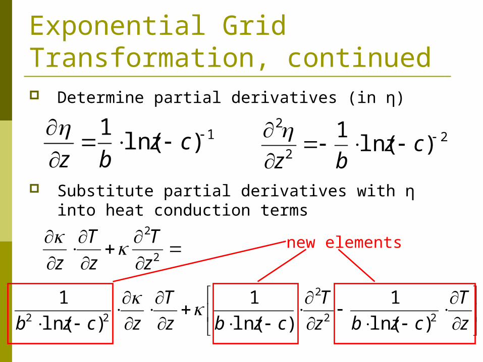
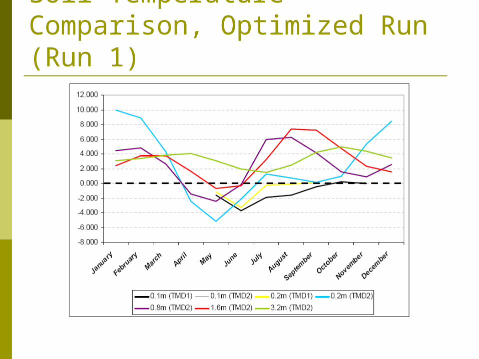