SOP TRANSACTIONS ON APPLIED PHYSICSISSN(Print): 2372-6229 ISSN(Online): 2372-6237

DOI: 10.15764/APHY.2014.03003Volume 1, Number 3, September 2014

SOP TRANSACTIONS ON APPLIED PHYSICS

Vibrational Modes in Acoustic GalleryScanning Probe MicroscopyHsien-Chih Hung1, Andres H. La Rosa1*, Rodolfo Fernandez1, Bret Comnes1,Richard Nordstrom2

1 Physics Department, Portland State University, P.O. Box 751, Portland, Oregon 972072 Mechanical Engineering and Materials Science Department, Portland State University, P.O. Box 751, Portland, Oregon 97207*Corresponding author: andres@pdx.edu

Abstract:A distinct characteristic in Acoustic Gallery Scanning Probe Microscopy (AG-SPM) constitutesthe use of its supporting structural frame as an acoustic resonant cavity for monitoring thenanometer-sized amplitude of its stylus-probe. Although very straightforward in its implementa-tion, its amplitude detection sensitivity could be improved by a more thorough understanding ofits working principle mechanism, as well as by a more systematic procedure to attain a closermatching between one of the cavitys acoustic resonances and the probes natural frequency.Herein, a description of the working principle of the AG-SPM is attempted from a vibrational-mode analysis perspective, and a successful specific procedure is presented to maximize theAG acoustic response. Such an improvement in sensitivity will make AG-SPM a better metrologyinstrumentation to study probe-sample shear-force interactions at nanometer scale separationdistances, as well as its role in the fabrication of nanostructures via SPM.

Keywords:Acoustic Feedback; SPM; Acoustic Gallery Sensing; Vibrational Modes; Tuning Fork

1. INTRODUCTION

There exists an interest for developing opto/acoustic imaging devices and sensors, which can be appliedin diverse areas including medicine and electronics [1, 2]. As the current trend of shrinking devicescontinues, detecting the wave-amplitude of the probing radiation with high sensitivity becomes crucial.Among the diverse strategies to achieve low signal levels detection, it is worth mentioning the effort toharness the confinement of waves into reduced spaces to, thus, more efficiently exploit their constructiveinterference. One way of achieving such a confinement is to use “perfect mirrors” whose working principleis based on the total internal reflection principle (different than the one that uses Bragg reflection as occursin dielectric-coated parallel mirrors). This method works over a broader range of frequencies, and can beused to make resonators confined in three-dimensions, provided one can force the wave inside the cavityto efficiently interfere with themselves [3, 4]. This approach is being pursued to build opto-mechanicalresonators [5], directional optical lasers[6], including nanodevices used in frontier research areas forcooling opto-mechanical systems at quantum levels [7, 8]. The work presented herein addresses the

22

Vibrational Modes in Acoustic Gallery Scanning Probe Microscopy

wave confinement strategy from an acoustic perspective. More specifically, we focus on attaining afurther development of Acoustic Gallery Scanning Probe Microscopy (AG-SPM) [9], a technique recentlyintroduced by our group, where the oscillatory motion of its tuning fork probe is tracked with an acoustictransducer located away from the probe. In AG-SPM the acoustic waves generated (at the probe-cavityjunction ) by its dithering probe end up confined on the walls of its structural supporting frame (thelatter resembling closer a cavity of cylindrical shape). By judiciously placing an acoustic transducer onthe perimeter of the cavity for maximum signal detection, AG-SPM is able to monitor the nanometer-size oscillations of its sturdy piezoelectric tuning fork probe. In this article we report efforts aimed atobtaining a better analytical understanding of the AG-SPM working principle, as well as investigating newstrategies for improving its detection sensitivity. The goal is making AG-SPM to become not only a moreeffective SPM imaging instrumentation, but also an analytical apparatus to characterize the propertiesof mesoscopic fluids confined between two solid boundaries, which appear to play a relevant role ininterfacial friction phenomena [10], as well as in the fabrication of nanostructures[11]. In order to gaina better perspective of the technique, we provide first a brief background about how the AG-SPM ideagerminated.

1.1 Acoustic Gallery Scanning Probe Microscopy

Scanning probe microscopy (SPM) comprises a collection of proximal-probe imaging techniqueswidely used to characterize the surface of materials with nanometer scale resolution. The workingprinciple of SPM-imaging is based on its ability to raster scan a surface with a sharp tip probe. To performthis detailed excursion, the tip is mounted to a voltage-controlled XYZ piezoelectric-positioner goingaround the contours of the sample’s topographic features. Oscillatory-voltages Vx and Vy are applied toexecute a pre-determined lateral motion, while an automated feedback voltage-control (that respond to aspecific device and mechanism that senses the probe-sample distance, as will be described below) dictatesthe proper Vz actuation. The latter allows to move the tip up and down, but maintaining its close proximityto the sample’s surface landscape. The recorded Vx, Vy and feedback Vz voltages are used to reconstruct,via software, the sample’s topographic image z = z(x,y) after a proper voltage-displacement calibrationof the voltages and XYZ-positioner displacements. A sharper probe leads to a finer image resolution.

To sense the probe sample-distance (required to implement the feedback control mentioned above) oneparticular type of SPM uses a quartz tuning fork (QTF) of 32.768 kHz nominal resonance frequency, whichhas a very stiff spring constant (⇠ 25,000 N/m) and has very low damping characteristics (mechanicalquality factor Q ⇠ 2000 or higher at ambient conditions). In this SPM, a sharp stylus is attached to one ofthe TF tines (typically oriented vertically); upon applying a driving voltage, the probe oscillates laterally(⇠ 1 nm amplitude) and the tuning fork, due to its piezoelectric characteristics, gives rise to an ac-current.The latter is synchronously detected with a lock-in amplifier [10]. It turns out that the amplitude of theprobe’s lateral oscillations decreases monotonically as the tip travels vertically towards the horizontallyoriented surface. The physics principles governing probe-sample shear-force interactions is not yet wellunderstood, however, the method is widely exploited to implement a Vz feedback voltage to controlthe probe-sample distance by simply monitoring the probe’s oscillations. Because of the mechanicalrigidity of the setup along the vertical direction, the probe does not experience sudden jumps towards thesample, as occurs in typical AFMs, thus providing well-controlled probe-sample distance. The latter is avery important metrology feature for studying the distance dependence of shear-force interactions. InQTF-SPM the vertical position of the probe is monitored by detecting the electrical admittance whiledriving the TF at its expected mechanical resonance. However, the TF’s intrinsic capacitance convolutes

23

SOP TRANSACTIONS ON APPLIED PHYSICS

the electrical admittance detection; as a result, it is not possible to determine directly the exact state ofTF’s mechanical motion. The latter compromises the metrology capabilities of the technique. Whilecorrections to suppress this shortcoming have been introduced,[12] it is highly desirable to design muchsimpler TF-based detection methods.

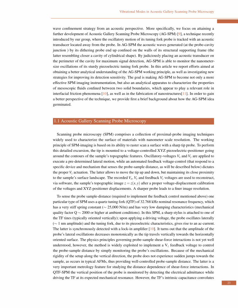
AG-SPM [9] offers an alternative to circumvent the shortcomings associated with the TF’s inherentcapacitance by relying instead in an acoustic transducer to monitor the oscillatory motion of a SPM probe.As schematically illustrated in Figure 1, the simplicity of AG consists in using its own supporting frameas an acoustic cavity where the mechanical waves, generated at the TF-cavity junction and subsequentlytravelling towards the cavity, are detected by an acoustic transducer judiciously located at the periphery ofthe cavity. AG is able to detect the TF tines’ lateral motion with nanometer-sized amplitude precision.Notice that this detection method resembles the ability to hear whisper conversations at the galleries of acathedral even when the source is located at extraordinary distances [13].

Although very straightforward in its implementation, AG-SPM would benefit from a better analyticaldescription of its working principle, which could eventually lead to better implementation strategies andfind out the condition of maximum detection sensitivity. Aware of the multiple bulk and surface wavesthat can be excited in a given non-homogeneous and non-symmetrical cavity, AG-SPM will be tested, asa first step, with cavities of different shape but maintaining some degree of cylindrical symmetry. Thedimension of cavities will be kept very similar; and an attempt will be made to describe the acousticspectral response from the existent analytical models. On the other hand, since AG-SPM relies on anideally perfect matching between the cavity’s resonance frequency and the probe’s mechanical resonancefrequency, which seldom occurs, we describe a method to overcome this shortcoming and, hence, improveAG-SPM detection sensitivity.

2. EXPERIMENTAL SETUP

Figure 1 shows the experimental setup for acoustically monitoring the nanometer-sized oscillations ofa probe attached to an electrically driven tuning fork. The setting has been described previously with verymuch detail [9]; herein we provide just a succinct description, accompanied with additional informationof some modifications introduced to independently test the frequency response of the cavity alone, as wellas improvements in the data acquisition process via LabVIEW, as shown in the bottom-left diagram ofFigure 2.

2.1 Characterization of the Cavity’s Mechanical Response

The left side of the top diagram in Figure 2 shows an electrically driven piezoelectric plate (12 mm⇥12mm⇥2 mm) that is used to mechanically excite the cavity in the 20 kHz to 40 kHz range (as to includethe 32.768 kHz TF’s operating frequency) while simultaneously monitoring its acoustic spectral response.The right side of the diagram shows an alternative way to excite the cavity by using an electrically drivenTF instead. In this last setting, the TF is held by a piezoelectric tube 1 and, altogether, attached to a

1 Piezo tube from EBL Products, Inc. EBL 3, 0.5 mm thick, 40 mm long, 20 mm outside diameter.

24

Vibrational Modes in Acoustic Gallery Scanning Probe Microscopy

Figure 1. Left: Schematic views of the acoustic gallery (AG) experimental setup for sensing the nanometer-sizedlateral vibrations amplitude of a sharp stylus that is attached to an electrically driven piezoelectric tuningfork (1). As the tip vibrates, the tube that holds the TF picks up mechanical waves, which travel towardsthe cavity where they interfere. An acoustic transducer (2) is judiciously placed on the periphery of thecavity, at a site of maximum constructive interference. Right: Synchronous detection of acoustic wavesvia a lock-in amplifier (4) referenced to the TF driving frequency. The simultaneous detection of the TF’selectrical admittance is optional.

Figure 2. Top: Typical size of the cavities analyzed herein. The excitation is either with a piezo-plate (PP) (left sidediagram) or with a tuning fork (TF) (right side diagram). Bottom right: Schematic of the experimentalsetup for testing the frequency response, where the cavity is excited no by a TF (as in Figure 1) but insteadby an electrically driven piezoelectric plate. Bottom-left: Typical acoustic spectral response in magnitude(trace with circles) and phase (solid trace).

stainless steel cylindrical cavity shell but electrically isolated by a disk made of macor ceramic material2. The piezoelectric tube plays here no other role than as a holder of the TF and as a medium throughwhich the TF vibrations are transmitted to the steel cavity. Alternatively, in this second experimentalsetting (top right side of Figure 2) the TF is interchanged, back and forth, with a piezoelectric plateas the excitation source. This is done intentionally to test the cavity’s spectral response each time thenatural frequency of the tuning fork is purposely varied by a few Hertz (as described in more detail in the“Matching Frequency” section below). The bottom-right side shows the lock-in synchronous detection of

2 MACOR Machinable Glass Ceramic is a registered trademark of Corning Incorporated, Corning, NY. MACORis composed of approximately 55% fluorophlogopite mica and 45% borosilicate glass. Youngs Modulus (at 25 ˚ C)equal to 66.9 GPa, DC volume resistivity (at 25 ˚ C) greater than 1016 ohm-cm.

25

SOP TRANSACTIONS ON APPLIED PHYSICS

Figure 3. Stainless-steel cylindrical shells used in the present work as acoustic cavities. The scale bar is 2.5 cm.

the acoustic signal, where the driving signal generator is interfaced via GPIB and controlled by LabViewgraphic program interface. The bottom-left side of the figure displays a typical acoustic spectral response;an ideal cavity would have a significant acoustic response at the particular TF operating frequency.

We can identify four main components in Figure 1 and Figure 2: (i) A driven element, which inFigure 1 is constituted by a piezoelectric TF of 32.768 kHz nominal resonance frequency and in Figure2 by a piezoelectric plate. A signal generator (SR DS-345) supplies a programmable frequency andprogrammable ac voltage amplitude to the piezoelectric element. (ii) An acoustic cavity, which is inmechanical contact with the TF or the piezo-plate. (iii) An acoustic transducer (DECI SE 25–P 426 thathas a 3 mm diameter sensitive area) placed at the periphery of the cavity. (iv) A lock-in amplifier (SR-844or SR-850) for synchronously detecting the acoustic signal; unless noted otherwise, we typically used a30 ms time constant. In a typical procedure, an ac-voltage of 10 mV rms amplitude is applied across theterminals of the TF, which makes the tines to laterally oscillate with a few nanometers amplitude (⇠ 4 nmwhen driven at its resonance frequency). The vibrations of the TF or the piezo-plate, respectively, aretransmitted as acoustic waves to the circular frame, where, we expect, they establish sites of constructiveinterference around the cavity’s periphery; the maxima are detected by the acoustic transducer via lock-insynchronous detection. In the case of Figure 2, the process is automated via LabVIEW and using aGeneral Purpose Interface Bus (to control of the signal generator settings) and a data acquisition card(NI 6008 DAQ). Additionally, for control and comparison purposes, the system also monitors the TF’selectrical admittance.

2.2 The Acoustic Cavity

Figure 3 displays circular (A, D) and regular hexagonal (C, D) stainless-steel cylindrical-shell cavitiesused in these experiments; Table 1 shows their corresponding dimensions. Cavities C and D have taperedexternal walls. The planar geometry of the external walls in B and C aimed at optimizing their contactarea with the flat sensitive area of the acoustic sensor. A plastic spring clamp is used to keep a tightcontact between the transducer and the cylindrical cavity 3, and a minute amount of vacuum-grease layeris sandwiched between the sensor and the cavity-wall in order to improve the acoustic coupling. Thenotches on the cavities A and B respond to the fact that they are already part of a SPM system, and have

3 We tried a variety of clamps of different spring constant, since pressing the acoustic sensor against the cavity tootight or too lose leads to a very poor coupling of sound from the cavity to the acoustic transducer.

26

Vibrational Modes in Acoustic Gallery Scanning Probe Microscopy

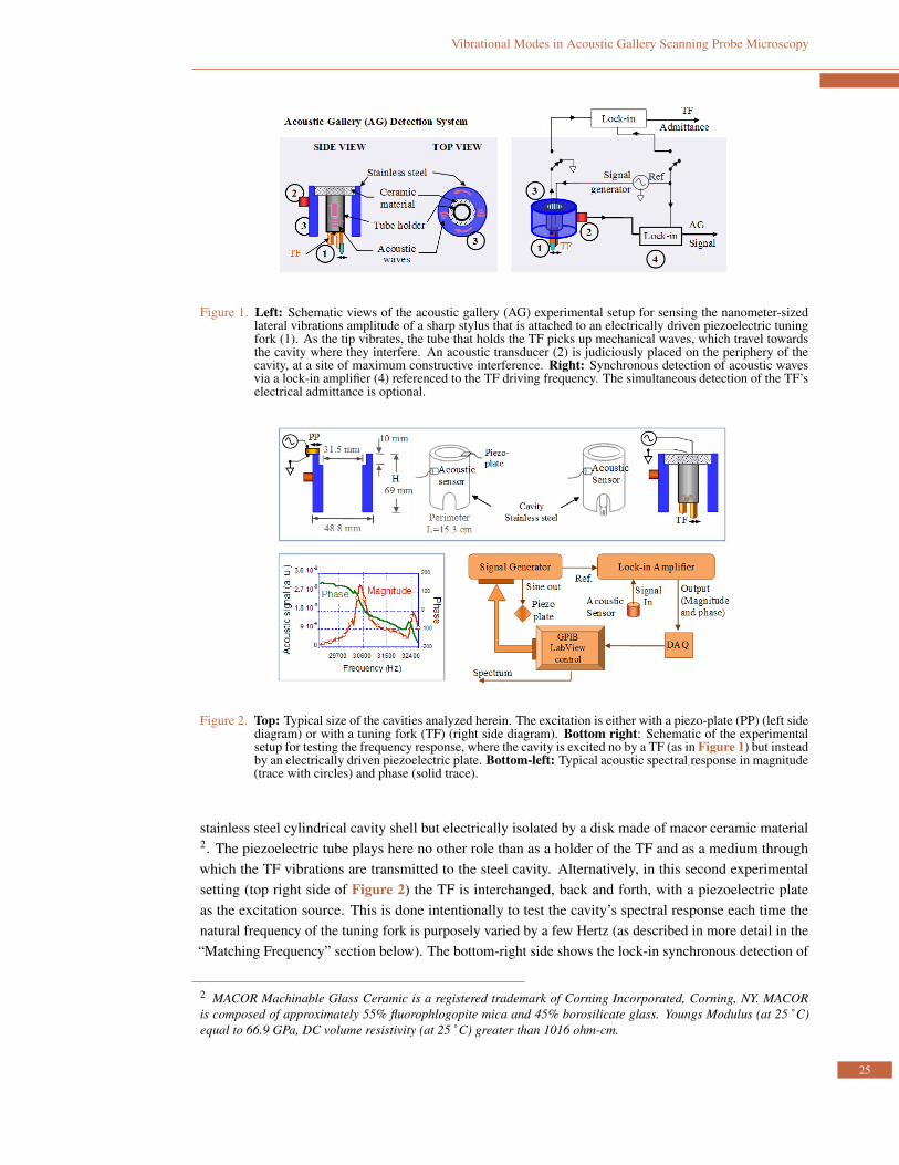
just been taken apart for analysis purposes. Notice, the test cavities were designed with slightly differentshapes and very similar sizes so any of them could relatively easy be integrated into an existent SPM.

Table 1.

Cavity ACircular

Cavity A’Circular

Cavity BHexagonal exter-nal walls

Cavity CHexagonal and tapered ex-ternal walls

Cavity DConical external walls

External diameter 48.8 mm 50.8 mm 31 mm(Top edge)51 mm (Bottom edge)

External perime-ter

153 mm 159.6 mm 145 mm 148 mm(Top side)168 mm (Bottom side)

97.5 mm(Top side)160 mm (Bottom side)

Internal diameter 31.5 mm 31.5 mm 31.5 mm 31.5 mm 25.4 mmInternal perimeter 99 mm 99 mm 99 mm 99 mm 79.8 mmHeight 69 mm 69 mm 69 mm 69 mm

2.3 Calibration of Piezoelectric TF’s Resonant Frequency

Once the spectral response of a given cavity is determined, it would be ideal that the resonancefrequency of the TF (with a probe attached to it) matches one of the acoustic spectral peaks; howeverthis seldom happens. This is aggravated by the fact that when a probe is attached to one of the tine ofthe TF, the resulting resonance frequency of the (TF + probe) system depends on many parameters suchas attachment procedure, length of the stylus probe, etc. To address this situation, we have establisheda very simple method to tune the TF’s resonance frequency (within a 2 kHz range), which consists inmodifying slightly its mass by adding a tiny amount of ethyl cyanoacrylate adhesive 4 to the side of oneof the tines. This procedure causes a “red shift” of the resonance frequency, and, since a cavity spectrumdisplays so many peaks, it is usually possible to find one of lower frequency than the initial TF’s naturalfrequency. The procedure is also accompanied by a decrease of the probe’s oscillation amplitude due todamping effect from the viscous glue; but we demonstrate herein that such loss is more than compensatedby the increase of acoustic signal when the modified TF’s natural frequency matches the cavity maximumresponse.

3. EXPERIMENTAL RESULTS

3.1 Acoustic Spectral Response From Cylindrical Cavity Shells

Figure 4 shows three superimposed spectra obtained by placing the acoustic sensor at different locationsaround the perimeter of the cavity, respectively. Notice, when the sensor is located at a particular positionon the periphery of the cavity we may obtain a high acoustic response at a given frequency, but the

4 Ethyl cyanoacrylate adhesive, better known as super glue. This adhesive was chosen because it requires only 30minutes waiting period between trials in order to obtain a reproducible result.

27

SOP TRANSACTIONS ON APPLIED PHYSICS

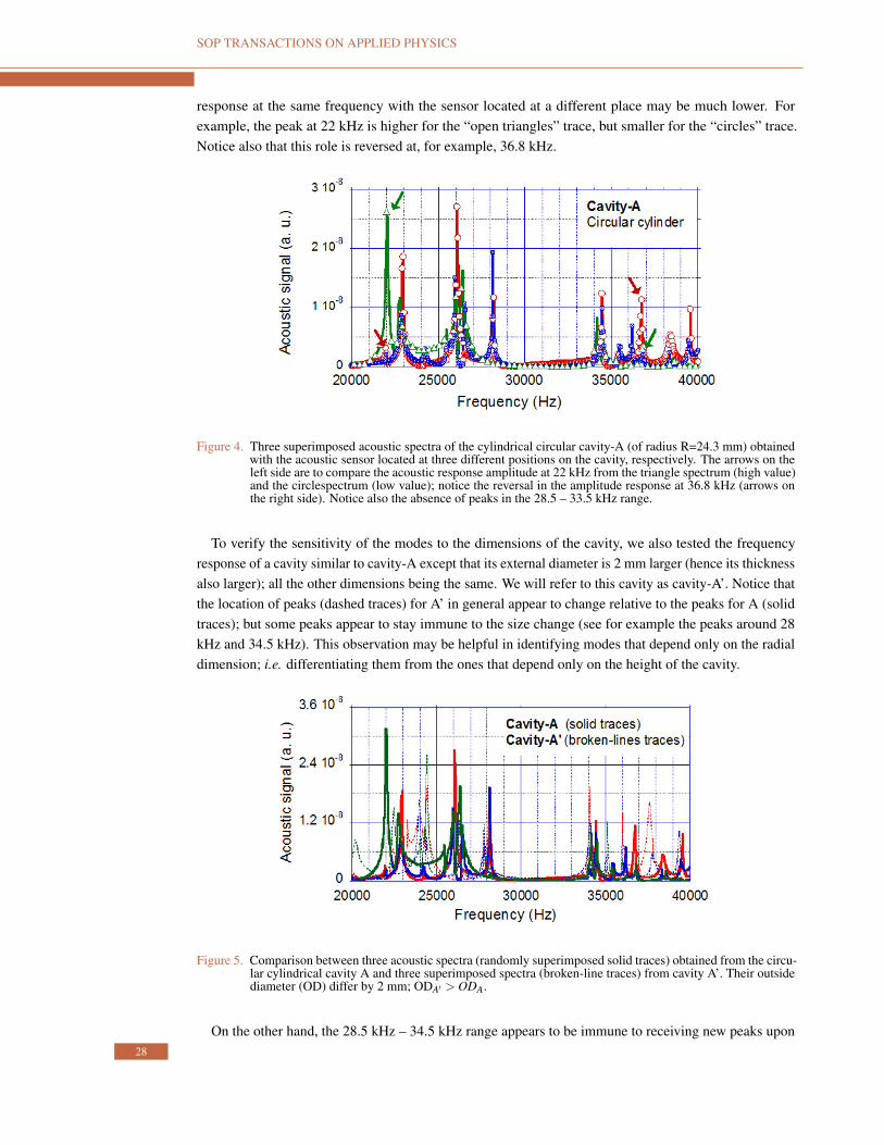
response at the same frequency with the sensor located at a different place may be much lower. Forexample, the peak at 22 kHz is higher for the “open triangles” trace, but smaller for the “circles” trace.Notice also that this role is reversed at, for example, 36.8 kHz.

Figure 4. Three superimposed acoustic spectra of the cylindrical circular cavity-A (of radius R=24.3 mm) obtainedwith the acoustic sensor located at three different positions on the cavity, respectively. The arrows on theleft side are to compare the acoustic response amplitude at 22 kHz from the triangle spectrum (high value)and the circlespectrum (low value); notice the reversal in the amplitude response at 36.8 kHz (arrows onthe right side). Notice also the absence of peaks in the 28.5 – 33.5 kHz range.

To verify the sensitivity of the modes to the dimensions of the cavity, we also tested the frequencyresponse of a cavity similar to cavity-A except that its external diameter is 2 mm larger (hence its thicknessalso larger); all the other dimensions being the same. We will refer to this cavity as cavity-A’. Notice thatthe location of peaks (dashed traces) for A’ in general appear to change relative to the peaks for A (solidtraces); but some peaks appear to stay immune to the size change (see for example the peaks around 28kHz and 34.5 kHz). This observation may be helpful in identifying modes that depend only on the radialdimension; i.e. differentiating them from the ones that depend only on the height of the cavity.

Figure 5. Comparison between three acoustic spectra (randomly superimposed solid traces) obtained from the circu-lar cylindrical cavity A and three superimposed spectra (broken-line traces) from cavity A’. Their outsidediameter (OD) differ by 2 mm; ODA0 > ODA.

On the other hand, the 28.5 kHz – 34.5 kHz range appears to be immune to receiving new peaks upon28

Vibrational Modes in Acoustic Gallery Scanning Probe Microscopy

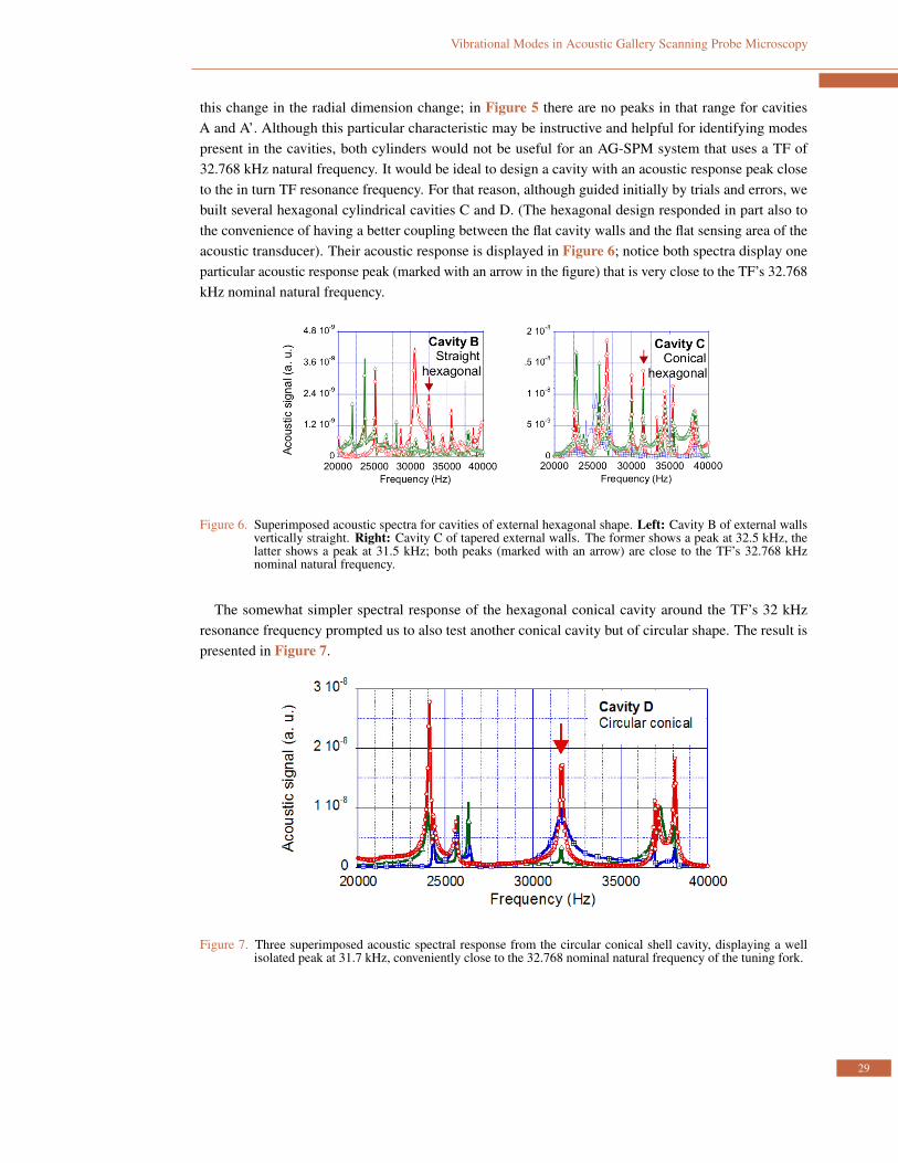
this change in the radial dimension change; in Figure 5 there are no peaks in that range for cavitiesA and A’. Although this particular characteristic may be instructive and helpful for identifying modespresent in the cavities, both cylinders would not be useful for an AG-SPM system that uses a TF of32.768 kHz natural frequency. It would be ideal to design a cavity with an acoustic response peak closeto the in turn TF resonance frequency. For that reason, although guided initially by trials and errors, webuilt several hexagonal cylindrical cavities C and D. (The hexagonal design responded in part also tothe convenience of having a better coupling between the flat cavity walls and the flat sensing area of theacoustic transducer). Their acoustic response is displayed in Figure 6; notice both spectra display oneparticular acoustic response peak (marked with an arrow in the figure) that is very close to the TF’s 32.768kHz nominal natural frequency.

Figure 6. Superimposed acoustic spectra for cavities of external hexagonal shape. Left: Cavity B of external wallsvertically straight. Right: Cavity C of tapered external walls. The former shows a peak at 32.5 kHz, thelatter shows a peak at 31.5 kHz; both peaks (marked with an arrow) are close to the TF’s 32.768 kHznominal natural frequency.

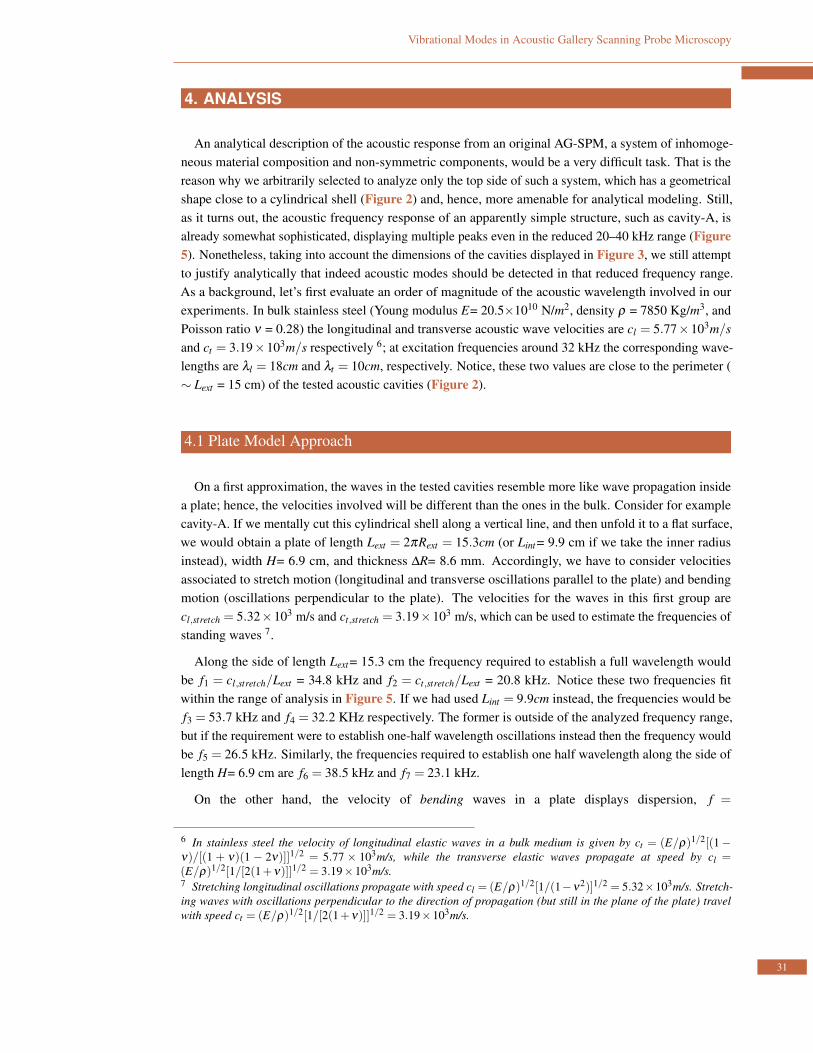
The somewhat simpler spectral response of the hexagonal conical cavity around the TF’s 32 kHzresonance frequency prompted us to also test another conical cavity but of circular shape. The result ispresented in Figure 7.

Figure 7. Three superimposed acoustic spectral response from the circular conical shell cavity, displaying a wellisolated peak at 31.7 kHz, conveniently close to the 32.768 nominal natural frequency of the tuning fork.

29

SOP TRANSACTIONS ON APPLIED PHYSICS

Figure 8. Superimposed spectral response of cavity-D (solid traces) obtained using a piezo-plate as excitation source(magnitude indicated on the left vertical scale). The diamond trace indicates the peak values of the cavityresponse acquired using a TF as the excitation source; each discrete data point corresponds to a TF tunedto a different natural frequency (magnitude of the signal indicated on the right vertical scale).

3.2 Matching Frequency

Next we use a piezoelectric tuning fork to excite the acoustic cavity (see top diagram in Figure 2). TheTF is firmly attached to a piezoelectric tube, and both together assembled to the cavity, constituting asetting that is very similar to the original SPM system, which inspired the AGS idea [9]. Since, in general,a cavity’s peak frequency response does not match the TF’s natural frequency, we proceeded to fine tunethe natural frequency of the TF in order to maximize the cavity’s acoustic response. We selected cavity-Dfor this principle demonstration given its isolated peak frequency response at 31.7 kHz, which facilitatestracking its acoustic response as the tuning fork’s natural frequency is purposely changed.

The procedure consists in applying a small drop of ethyl cyanoacrylate adhesive 5 to one of the TF-tines,which typically produces a “red shift” change between 50 Hz to 200 Hz (a decrease in the magnitudeof the TF oscillation is also observed). A 10-minute drying time ensures a reproducible measurementof the frequency change. The “diamond” trace in Figure 8 summarizes the result of this procedure afterimplementing it several times. For further control and comparison purposes, after each addition of masswe also recorded the cavity’s spectral response but using a piezo plate as the driving source. For thispurpose, the piezo-plate interchanged position with the TF. However, changing a given source back andforth creates some degree of variations in the acoustic response. We therefore graph multiple spectralresponses, which were taken after each interchange of excitation source. Put all together we observe inFigure 8 (left scale) that the different spectra display a similar trend. This whole procedure allows us totune the TF natural frequency beyond a 2 kHz range.

5 Ethyl cyanoacrylate adhesive, better known as super glue. This adhesive was chosen because it requires only 30minutes waiting period between trials in order to obtain a reproducible result.

30

Vibrational Modes in Acoustic Gallery Scanning Probe Microscopy

4. ANALYSIS

An analytical description of the acoustic response from an original AG-SPM, a system of inhomoge-neous material composition and non-symmetric components, would be a very difficult task. That is thereason why we arbitrarily selected to analyze only the top side of such a system, which has a geometricalshape close to a cylindrical shell (Figure 2) and, hence, more amenable for analytical modeling. Still,as it turns out, the acoustic frequency response of an apparently simple structure, such as cavity-A, isalready somewhat sophisticated, displaying multiple peaks even in the reduced 20–40 kHz range (Figure5). Nonetheless, taking into account the dimensions of the cavities displayed in Figure 3, we still attemptto justify analytically that indeed acoustic modes should be detected in that reduced frequency range.As a background, let’s first evaluate an order of magnitude of the acoustic wavelength involved in ourexperiments. In bulk stainless steel (Young modulus E= 20.5⇥1010 N/m2, density r = 7850 Kg/m3, andPoisson ratio n = 0.28) the longitudinal and transverse acoustic wave velocities are cl = 5.77⇥103m/sand ct = 3.19⇥103m/s respectively 6; at excitation frequencies around 32 kHz the corresponding wave-lengths are ll = 18cm and lt = 10cm, respectively. Notice, these two values are close to the perimeter (⇠ Lext = 15 cm) of the tested acoustic cavities (Figure 2).

4.1 Plate Model Approach

On a first approximation, the waves in the tested cavities resemble more like wave propagation insidea plate; hence, the velocities involved will be different than the ones in the bulk. Consider for examplecavity-A. If we mentally cut this cylindrical shell along a vertical line, and then unfold it to a flat surface,we would obtain a plate of length Lext = 2pRext = 15.3cm (or Lint= 9.9 cm if we take the inner radiusinstead), width H= 6.9 cm, and thickness DR= 8.6 mm. Accordingly, we have to consider velocitiesassociated to stretch motion (longitudinal and transverse oscillations parallel to the plate) and bendingmotion (oscillations perpendicular to the plate). The velocities for the waves in this first group arecl,stretch = 5.32⇥103 m/s and ct,stretch = 3.19⇥103 m/s, which can be used to estimate the frequencies ofstanding waves 7.

Along the side of length Lext= 15.3 cm the frequency required to establish a full wavelength wouldbe f1 = cl,stretch/Lext = 34.8 kHz and f2 = ct,stretch/Lext = 20.8 kHz. Notice these two frequencies fitwithin the range of analysis in Figure 5. If we had used Lint = 9.9cm instead, the frequencies would bef3 = 53.7 kHz and f4 = 32.2 KHz respectively. The former is outside of the analyzed frequency range,but if the requirement were to establish one-half wavelength oscillations instead then the frequency wouldbe f5 = 26.5 kHz. Similarly, the frequencies required to establish one half wavelength along the side oflength H= 6.9 cm are f6 = 38.5 kHz and f7 = 23.1 kHz.

On the other hand, the velocity of bending waves in a plate displays dispersion, f =

6 In stainless steel the velocity of longitudinal elastic waves in a bulk medium is given by ct = (E/r)1/2[(1�n)/[(1 + n)(1 � 2n)]]1/2 = 5.77 ⇥ 103m/s, while the transverse elastic waves propagate at speed by cl =(E/r)1/2[1/[2(1+n)]]1/2 = 3.19⇥103m/s.7 Stretching longitudinal oscillations propagate with speed cl = (E/r)1/2[1/(1�n2)]1/2 = 5.32⇥103m/s. Stretch-ing waves with oscillations perpendicular to the direction of propagation (but still in the plane of the plate) travelwith speed ct = (E/r)1/2[1/[2(1+n)]]1/2 = 3.19⇥103m/s.

31

SOP TRANSACTIONS ON APPLIED PHYSICS

Figure 9. Cross sections and coordinates to describe axisymmetric vibration modes in a cylindrical shell.

(k2/2p)p

E/rp

h2/ [12(1� v2)], the frequency being proportional to k2 instead of k as occur in thecase of stretching waves. A mode with one-half wavelength fitting along Lext would have f = 0.887⇥103

Hz. Notice the frequencies of the lowest bending waves frequencies are much smaller than the lowestfrequencies associated to the stretching waves; this is expected since, by comparison, the plate offers lessresistance to bending than to stretching elongations. Among the higher modes that can be calculated withthe previous expression, only f8 = 31.9 kHz fits inside our range of analysis 8 . If we use Lin instead, weobtain f9 = 33.9 kHz 9; and along the side of length H = 6.9 cm we obtain f9 = 39 kHz 10.

Overall, we have found up to nine potential standing wave modes whose frequencies fit within the 20kHz - 40 kHz bandwidth in which cavity-A was tested. But some of the individual frequencies are notreproduced experimentally, which is an indication that the flat plate model needs some refinement.

4.2 Axisymmetric Free Vibrations

A better approximation can be obtained from analytical solutions associated to waves established in thincylindrical shells (of radius R, height L, and thickness h). An important feature of shells, that distinguishthem from plates, is that bending is accompanied with stretching; that is deformation of plates whichare curved in the undeformed state have properties that are fundamentally different from those of flatplates [14]. It is worth then to explore analytical solutions describing vibrations in cylindrical shells andto compare them with our experimental results. For simplicity, let’s consider first axisymmetric freevibrations (Figure 9), i.e. free flexural vibrations modes of the cylinder where the radial w displacementsdo not depend on the polar coordinate q , and have zero circumferential displacement p . Any crosssection of the cylinder will then be a circular ring, with several (n) half-waves established along theshell axis (only one half-wavelength is schematically shown on the left side of Figure 9). The equationgoverning these particular type of waves is given by[15] ∂ 4w/∂ z4 +4b 4w =�(rh/D)(∂ 2w/∂ t2), whereD ⌘ Eh3/12(1 � v2) is the flexural rigidity (or stiffness) of the shell, and b 4 ⌘ Eh/4R2D = 3(1�

8 The other bending mode frequencies along a side of length Lext = 15.3 cm are 3.55 kHz, 7.9 kHz, 14.2 kHz, 22.2kHz, and 31.9 kHz, 43.5 kHz.9 The other bending mode frequencies along a side of length Lin = 9.9 cm are 33.9 kHz, 53 kHz.10 The other bending mode frequencies along a side of length H = 6.9 cm are 4.36 kHz, 17 kHz, 39 kHz, 69 kHz.

32

Vibrational Modes in Acoustic Gallery Scanning Probe Microscopy

v2)/R2h2. This equation admits solutions of the form w(x, t) = sin(npz/L)sin(2p fnt) provided that,fn = (1/2pR)

p(E/r)

p1+µl 4

n , where µ = (h/R)2/12(1� v2) and ln = n(pR/L).

For cavity-A (of radius R = Rext = 24.4 mm, thickness h = 8.6 mm, and height L = 68.8 mm) we obtainf1 = 33.6 Hz and f2 = 37.6 Hz for n = 1 and n = 2 respectively. (For a 0.1 mm change in the radius, thecalculated frequency of a mode changes by about 150 Hz). Although these solutions correspond to aparticular boundary condition where the radial elongation w is zero at z= 0 and z = L, it turns out that forcylinders not too short (i.e. discarding those satisfying R/L > 1) the first mode at least is expected not tosignificantly depend on the boundary conditions [15]. Although the two frequencies calculated abovefall within our 20 kHz - 40 kHz range of analysis, still it is difficult (with such a partial information) tomatch them univocally with some particular experimental peaks displayed in Figure 5. For this reasonwe expand our analysis to check more sophisticated modes; those that depend on the polar coordinate.

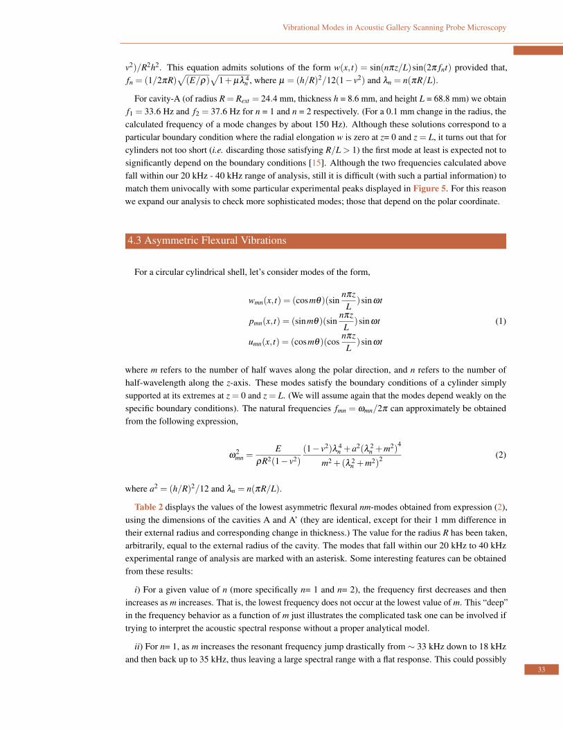
4.3 Asymmetric Flexural Vibrations

For a circular cylindrical shell, let’s consider modes of the form,

wmn(x, t) = (cosmq)(sinnpzL

)sinwt

pmn(x, t) = (sinmq)(sinnpzL

)sinwt

umn(x, t) = (cosmq)(cosnpzL

)sinwt

(1)

where m refers to the number of half waves along the polar direction, and n refers to the number ofhalf-wavelength along the z-axis. These modes satisfy the boundary conditions of a cylinder simplysupported at its extremes at z = 0 and z = L. (We will assume again that the modes depend weakly on thespecific boundary conditions). The natural frequencies fmn = wmn/2p can approximately be obtainedfrom the following expression,

w2mn =

ErR2(1� v2)

(1� v2)l 4n +a2(l 2

n +m2)4

m2 +(l 2n +m2)2 (2)

where a2 = (h/R)2/12 and ln = n(pR/L).

Table 2 displays the values of the lowest asymmetric flexural nm-modes obtained from expression (2),using the dimensions of the cavities A and A’ (they are identical, except for their 1 mm difference intheir external radius and corresponding change in thickness.) The value for the radius R has been taken,arbitrarily, equal to the external radius of the cavity. The modes that fall within our 20 kHz to 40 kHzexperimental range of analysis are marked with an asterisk. Some interesting features can be obtainedfrom these results:

i) For a given value of n (more specifically n= 1 and n= 2), the frequency first decreases and thenincreases as m increases. That is, the lowest frequency does not occur at the lowest value of m. This “deep”in the frequency behavior as a function of m just illustrates the complicated task one can be involved iftrying to interpret the acoustic spectral response without a proper analytical model.

ii) For n= 1, as m increases the resonant frequency jump drastically from ⇠ 33 kHz down to 18 kHzand then back up to 35 kHz, thus leaving a large spectral range with a flat response. This could possibly

33

SOP TRANSACTIONS ON APPLIED PHYSICS

Table 2. Fuzzy if-then rules

n m Cavity AFreq. (Hz)

Cavity A’Freq. (Hz)

1 0 33621 323931 1 18345 186301 2 18807 197201 3 34938* 36379*1 4 59381 615561 5 91082 942082 0 37668* 37534*2 1 34363* 35184*2 2 35782* 37914*2 3 49610 525572 4 73168 768922 5 104562 1092383 0 51662 544663 1 52599 559623 2 58449 628823 3 72817 781923 4 95935 1021833 5 126998 134231

Cavity A: Rext =24.4 mm; thickness = 8.6 mm. Cavity A: Rext =25.4 mm; thickness = 9.6 mm.

be one of the reasons why the spectrum in Figure 4 displays a flat response in the 28.5 kHz - 33.5 kHzrange.

iii) The modes for cavity-A marked with an asterisk in Table 2 have frequencies around 35 kHz, aregion where the spectrum in Figure 4 also shows several peaks. These peaks are located just at the rightside of the 28.5 kHz - 33.5 kHz range where there is a flat zero-response. With the exception of the modem = 0, the model predicts that the frequency should increase when comparing cavity-A and cavity-A’ 11.This is not in contradiction with the result in Figure 5 (where the peaks from cavity-A and cavity-A’ aresuperimposed), since the 28.5 kHz - 33.5 kHz range still has a flat zero-response (i.e. no peak moved to alower frequency, thus in agreement with what was predicted by the model).

Despite the consistency of the asymmetric flexural vibrations model with the results outlined above,expression (3) is still unable to predict the peak responses in the 20 kHz to 28.5 kHz range. One possiblereason may lie in the arbitrariness of using the external radius of the cavity as the value for R in expression(2) to calculate the values presented in Table 2. Maybe we should identify an affective radius (with avalue in between Rmax and Rmin). This is explored in Table 3, which lists the frequencies of the differentmodes corresponding to different radii, but keeping the thickness of the cavity constant. Notice that forradii values around R= 0.020 m (the average of Rmax and Rmin), the n= 1, m= 2 mode has frequencies inthe 21 kHz to 28 kHz range. But adopting any of these radii would prevent us from explaining the peaksaround and above 35 kHz. We are facing then the limitations of the model that is applicable only to thin

11 As the radius increases, the frequency of the mode in principle should rather decrease. But in the case of cavityA’ not only its radius increased but also its thickness. An increase in thickness makes the the cavity more robust andwith a higher resonance frequency.

34

Vibrational Modes in Acoustic Gallery Scanning Probe Microscopy

Table 3.

n m Freq (Hz)(Rin=0.0157 m)

Freq. (Hz)(R=0.018 m)

Freq. (Hz)(R=0.020 m)

Freq. (Hz)(R=0.022 m)

Freq. (Hz)(Rext =0.0244m)

1 0 51826 45397 40902 37229 336211 1 18205 18220 18312 18370 183451 2 35437 28545* 24366* 21367* 188071 3 77010 60069 49570 41818 349381 4 136124 105282 86143 71986 593811 5 212325 163609 133374 111005 910822 0 54538 48471 44289 40921 376682 1 41325 39397 37724 36132 343632 2 51654 45200 41273 38384 357822 3 91063 74279 63929 56326 496102 4 149696 118896 99804 85700 731682 5 225732 177029 146809 124458 1045623 0 64997 59997 56672 54080 516623 1 63100 59560 56953 54767 525993 2 76452 69531 65088 61662 584493 3 114384 97663 87313 79657 728173 4 172319 141572 122522 108450 959353 5 248074 199393 169195 146868 126998

shells with low thickness-to-radius ration, but in our case that factor is 0.35.

We have then reached a point in which we encounter very much limitations in the model used todescribe our experimental results, even though we have limited ourselves to analyze just a section of theAG-SPM hardware with the highest symmetry. We come to the conclusion that it may be more appropriateto use computer simulation, in which there will be no approximations in the model, and the calculationcan be compared with existent SPM stages.

5. CONCLUSIONS

The working principle mechanism of AG-SPM has been analyzed using as a model asymmetric flexuralvibrations in cylindrical shells. These modes would be excited by an electrically driven quartz tuningfork thus establishing localized maxima and minima acoustic vibrations around the SPM’s structuralframe, The model is chosen to fit the geometrical shape of the frame, which resembles closer a cylindricalshell cavity. Different cavities of gradually different sizes and shapes were tested. Despite their similardimensions (including two circular cavities whose radii differed by only 1 mm) and slightly differentshape (cylinders of straight or tapered external walls), we found that their experimental spectral acousticresponse displayed significant disparity among each other. The observed sensitivity of the spectralresponse to fine variations in the cavity dimensions is corroborated by the model, which for cavities ofcircular shape predicts changes in the resonance peaks of about 150 Hz for a 0.1 mm change in radius.For a cavity of 25 mm radius, this represents a change in 0.4 %. This fine sensitivity of the spectralresponse made difficult to identify and track analytically the multiple isolated peak responses due to therelatively coarse geometrical variations among the tested cavities. Still, the model predicted the existenceof resonant peaks within the experimentally analyzed 20 – 40 kHz range. The model also revealed that

35

SOP TRANSACTIONS ON APPLIED PHYSICS

the lowest resonant frequency does not occur at the lowest values of the mode indices n, m; instead as thevalue of m increases monotonically (for a fixed n) the corresponding discrete resonance frequencies firstdecrease drastically and then increase back again, thus leaving behind an empty frequency range gap. Asintricate as this latter feature may appear to be, it could be the reason why the spectral response from thecylindrical cavities A and A’ display a flat zero-response in the 28.5 kHz - 33.5 kHz range. Despite all themerits, as rationalized above, of the thin cylindrical cavity model used here, the observed high sensitivityof the spectral response to the cavity’s dimensions and shape suggests that more realistic models (ofnon-symmetric shape component and inhomogeneous material composition) are needed. It would bethen highly recommended to explore the use of numerical analysis as the next step in the investigation ofparticular modes existent in a given AG-SPM structural frame.

On the other hand, we have successfully been able to track the cavity response using different TFsof corresponding different natural frequencies as the driving sources. The response to the TF’s singlefrequency faithfully tracked the cavity’s spectral response. Retrospectively, based on these new results,it appears that the ASG-SPM has not been used very efficiently in the past. The method describedhere offers the possibility to gain a much higher sensitivity. The significance of these outcomes residesin the corresponding improvement in detection sensitivity of the AG-SPM to analyze more accuratelyprobe-sample shear-force interactions at nanometer separation distances.

References

[1] R. G. Maev, Advances in Acoustic Microscopy and High Resolution Imaging: From Principles toApplications. Wiley-VCH, 2013.

[2] W. Osten and N. Reingand, Optical Imaging and Metrology: Advanced Technologies. Wiley-VCH,2012.

[3] G. Hackenbroich and J. U. Nockel, “Dynamical tunneling in optical cavities,” EPL(EurophysicsLetters), vol. 39, no. 4, p. 371, 1997.

[4] J. Heebner, R. Grover, and T. Ibrahim, “Optical Microresonators: Theory, Fabrication, and Applica-tions,” Springer Series in Optical Sciences, 2010.

[5] M. Tomes and T. Carmon vol. 102, p. 113601, 2009.[6] Q. J. Wang, C. Yan, N. Yu, J. Unterhinninghofen, J. Wiersig, C. Pflugl, L. Diehl, T. Edamura,

M. Yamanishi, H. Kan, et al., “Whispering-gallery mode resonators for highly unidirectional laseraction,” Proceedings of the National Academy of Sciences, vol. 107, no. 52, pp. 22407–22412, 2010.

[7] A. Matsko, A. Savchenkov, V. Ilchenko, D. Seidel, and L. Maleki, “Optomechanics with surface-acoustic-wave whispering-gallery modes,” Physical Review Letters, vol. 103, no. 25, p. 257403,2009.

[8] T. J. Kippenberg and K. J. Vahala, “Cavity optomechanics: back-action at the mesoscale,” Science,vol. 321, no. 5893, pp. 1172–1176, 2008.

[9] A. H. La Rosa, N. Li, R. Fernandez, X. Wang, R. Nordstrom, and S. Padigi, “Whispering-galleryacoustic sensing: Characterization of mesoscopic films and scanning probe microscopy applications,”Review of Scientific Instruments, vol. 82, no. 9, p. 093704, 2011.

[10] K. Karrai and I. Tiemann, “Interfacial shear force microscopy,” Physical Review B, vol. 62, no. 19,p. 13174, 2000.

[11] X. Wang, X. Wang, R. Fernandez, M. Yang, and A. La Rosa J. Nanosci. Lett., vol. 2, p. 23, 2012.[12] R. D. Grober, J. Acimovic, J. Schuck, D. Hessman, P. J. Kindlemann, J. Hespanha, A. S. Morse,

K. Karrai, I. Tiemann, and S. Manus, “Fundamental limits to force detection using quartz tuning36

Vibrational Modes in Acoustic Gallery Scanning Probe Microscopy

forks,” Review of Scientific Instruments, vol. 71, no. 7, pp. 2776–2780, 2000.[13] A. Bate, “Note on the whispering gallery of St Paul’s Cathedral, London,” Proceedings of the

Physical Society, vol. 50, no. 2, p. 293, 1938.[14] L. Landau and E. Lifshitz, “Theory of Elasticity,” 2005.[15] E. Ventsel and T. Krauthammer, Thin Plates and Shells, Theory, Analysis, and Applications. Marcel

Dekker Inc., 2001.

37

About This Journal APHY is an open access journal published by Scientific Online Publishing. This journal focus on the following scopes (but not limited to): ¾ Biophysics and Biosensors ¾ Instrumentation and Metrology ¾ Magnetism ¾ Nanomaterials and Nanotechnologies ¾ Optical Manipulation

¾ Photonics ¾ Physics and Mechanics of Fluids, Microfluidics ¾ Physics of Energy Transfer, Conversion and

Storage

¾ Physics of Organic Materials and Devices ¾ Semiconductors and Devices ¾ Singular Optics ¾ Spectroscopy ¾ Spintronics ¾ Superconductivity

¾ Surfaces and Interfaces ¾ Thin Films

Welcome to submit your original manuscripts to us. For more information, please visit our website: http://www.scipublish.com/journals/APHY/ You can click the bellows to follow us: � Facebook: https://www.facebook.com/scipublish � Twitter: https://twitter.com/scionlinepub � LinkedIn: https://www.linkedin.com/company/scientific-online-publishing-usa � Google+: https://google.com/+ScipublishSOP

SOP welcomes authors to contribute their research outcomes under the following rules: ¾ Although glad to publish all original and new research achievements, SOP can’t bear any

misbehavior: plagiarism, forgery or manipulation of experimental data. ¾ As an international publisher, SOP highly values different cultures and adopts cautious attitude

towards religion, politics, race, war and ethics.

¾ SOP helps to propagate scientific results but shares no responsibility of any legal risks or harmful effects caused by article along with the authors.

¾ SOP maintains the strictest peer review, but holds a neutral attitude for all the published articles. ¾ SOP is an open platform, waiting for senior experts serving on the editorial boards to advance the

progress of research together.