Vibration control of maglev vehicles traveling over a...

ARTICLE IN PRESS

JOURNAL OFSOUND ANDVIBRATION

0022-460X/$ - s

doi:10.1016/j.js

�Tel.: +886

E-mail addr

Journal of Sound and Vibration 321 (2009) 184–200

www.elsevier.com/locate/jsvi

Vibration control of maglev vehicles traveling overa flexible guideway

J.D. Yau�

Department of Architecture, Tamkang University, 5, Lane 199, Kinghua Street, Taipei 10620, Taiwan

Received 20 April 2008; received in revised form 10 August 2008; accepted 11 September 2008

Handling Editor: J. Lam

Available online 11 November 2008

Abstract

As a series of maglev (magnetically levitated) vehicles travel over a flexible guideway with constant speeds, their

acceleration amplitudes will be amplified significantly at resonant or higher speeds. This paper intends to develop a neuro-

PI (proportional-integral) controller to control the dynamic response of the maglev vehicles around an allowable

prescribed acceleration. The maglev vehicle is simplified as a two-degree-of-freedom (two-dof) moving oscillator controlled

by an on-board PI controller and the guideway is modeled as a simply supported beam. Considering the motion-dependent

nature of electromagnetic forces working in a maglev system, this study presents an iterative approach to compute the

dynamic response of a maglev-oscillator/guideway coupling system based on the Newmark method. The proposed

neuro-PI controller is trained using back-propagation neural network in such a way that its PI gains are correlated

to the generated data set of moving speeds, mid-span acceleration amplitude of the guideway, and maximum

vertical accelerations of maglev oscillators. Numerical simulations demonstrate that a trained neuro-PI controller has the

ability to control the acceleration amplitude for running maglev vehicles within an allowable region of prescribed

acceleration.

r 2008 Elsevier Ltd. All rights reserved.

1. Introduction

The commercial operation of the Shanghai maglev transport system in 2002 marked the beginning of a newera in maglev transport system. Compared with traditional wheel/track transit vehicles, a high-speed maglevtrain can offer the advantages of low energy consumption, less environmental impact, as well as lower noiseand emissions. With the advanced maglev technology, powerful magnets are able to lift a vehicle up andpropel it forward along a guideway via electromagnetic forces. According to the suspension modes to guide amaglev train moving on guideways, two kinds of maglev technologies have been developed: (1)electromagnetic suspension (EMS, see Fig. 1(a)) with attractive mode; (2) electrodynamic suspension (EDS,see Fig. 1(b)) with repulsive mode [1–3]. The EMS system can lift a train up using attractive forces by themagnets beneath a guide-rail. The EDS system suspends a train above its guide-rail using magnetic repulsive

ee front matter r 2008 Elsevier Ltd. All rights reserved.

v.2008.09.030

2 23581830; fax: +886 2 23959041.

ess: [email protected]

www.elsevier.com/locate/jsvi

dx.doi.org/10.1016/j.jsv.2008.09.030

mailto:[email protected]

ARTICLE IN PRESS

Fig. 1. Schematic diagram of two maglev-vehicle systems: (a) electromagnetic suspension (EMS) and (b) electrodynamic suspension

(EDS).

J.D. Yau / Journal of Sound and Vibration 321 (2009) 184–200 185

forces to take the train off the U-shaped guideway. To suspend a maglev vehicle at a stable levitation gap (airgap) between the on-board levitation magnets and the guideway, a controllable electromagnetic field isgenerated in its maglev suspension system. Obviously, the response analysis of a maglev train moving on aflexible guideway is related to not only the dynamics of vehicle/guideway interaction but also the control of themaglev system.

With the recent development of high-speed rail in ground transportation, there are many literatureson the study of train-induced vibration of railway bridges [4–15]. One of the important findings in theseresearch works is that as a train travels over a bridge at resonant speeds, the response of the bridge tends toincrease steadily as there are more loads passing the bridge [5,6,9]. This is the so-called ‘‘resonancephenomenon’’ for rail bridges. However, relatively little research attention so far seems to conduct thedynamic interaction response of maglev trains running on guideways at resonant speeds. Cai and Chen [16]and Cai et al. [17] investigated the response characteristics of different maglev-vehicle models travelingover flexible guideways. They concluded that a concentrated-load vehicle model might result in largerresponses of both guideway deflections and vehicle accelerations than a distributed-load vehicle model.In the literature review works conducted by Cai and Chen [18], various aspects of the dynamic characteristics,magnetic suspension systems, vehicle stability, and suspension control laws for maglev/guidewaycoupling systems were discussed. Zheng et al. [19,20] presented two kinds of vehicle/guideway couplingmodels with controllable magnetic suspension systems to investigate the vibration behavior of a maglevvehicle running on a flexible guideway. They observed the phenomena of divergence, flutter, and collisionon the dynamic stability of a maglev-vehicle traveling on a flexible guideway. By simulating a magneticforce as an equivalent spring-dashpot system, Zhao and Zhai [21] modeled a TR06 carriage as a10-degree-of-freedom (10 dof) vehicle model with a rigid car body supported by four sets of magnetbogies to investigate the vertical random response and ride quality of a maglev vehicle traveling on elevatedguideways.

In this study, a simplified model of a two-dof maglev oscillator controlled by a PI controller [22–24] isemployed to simulate a maglev vehicle moving on a flexible guideway. The guideway is modeled asa simply supported beam. Based on the maglev theory, the maglev-oscillator system is lifted up abovethe guideway with a stable levitation gap via a motion-dependent electromagnetic force (see Fig. 1).By employing Galerkin’s method to convert the governing equations containing moving maglev oscillatorsinto two sets of generalized differential equations, the computation of dynamic response for thevehicle/guideway coupling system was carried out using an iterative approach [15] with Newmark’s bmethod [25]. To control the dynamic response of a series of maglev oscillators running on a flexibleguideway with various speeds, a neuro-PI controller based on back-propagation algorithm [26,27] isdeveloped, in which it can provide suitable control gains in reducing the response of maglev oscillators.Numerical simulations indicate that the dynamic response of maglev vehicles traveling over a flexibleguideway at resonant speed can be restricted to a preset acceleration using the proposed neuro-PIcontroller.

ARTICLE IN PRESSJ.D. Yau / Journal of Sound and Vibration 321 (2009) 184–200186

2. Formulation

2.1. Basic considerations

Generally, the lateral flexural stiffness of a guideway is much larger than the vertical one. For this reason,the lateral vibrations of the guideway due to moving maglev vehicles will also be smaller than the verticalmotions. To simplify the formulation of vehicle/guideway interaction with the maglev system, only verticalvehicle motion is considered in this study because it can dominate the dynamic behavior of vehicle/guidewayinteractions [17]. The following are the assumptions adopted for the maglev-vehicle/guideway system:

(1)
The flexible guideway is modeled as a linear elastic Bernoulli–Euler beam with uniform cross-section. (2) A maglev train passing over the guideway is modeled as a sequence of identical maglev vehicles with equal
intervals.
(3) The maglev vehicle is modeled as a one-dimensional and two-dof oscillator model that consists of two
concentrated masses, with the top one representing the mass lumped from the car body and the bottomone the mass of a magnetic wheel-set.

(4)
The effect of time delay between the input voltage and the output current on a maglev suspension system isnegligible.
2.2. Governing equations of motion

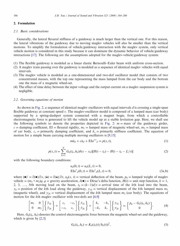
As shown in Fig. 2, a sequence of identical maglev oscillators with equal intervals d is crossing a single-spanflexible guideway at constant speed v. The maglev-oscillator model is composed of a lumped mass (car body)supported by a spring-dashpot system connected with a magnet bogie, from which a controllableelectromagnetic force is generated to lift the vehicle model up at a stable levitation gap. Here, we shall usethe following symbols to denote the properties depicted in Fig. 2: m ¼ mass of the guideway girder,c ¼ damping coefficient, EI ¼ flexural rigidity, m1 ¼ lumped mass of magnetic wheel-set, m2 ¼ lumped massof car body, cv ¼ primarily damping coefficient, and kv ¼ primarily stiffness coefficient. The equation ofmotion for a simple beam carrying multiple moving oscillators is [9,15]

m €ud þ c _ud þ EIu0000d ¼ pðx; tÞ, (1)

pðx; tÞ ¼XN

k¼1

Gkðik; hkÞdðx� xkÞ½Hðt� tkÞ �Hðt� tk � L=vÞ� (2)

with the following boundary conditions:

udð0; tÞ ¼ udðL; tÞ ¼ 0,

EIu00dð0; tÞ ¼ EIu00dðL; tÞ ¼ 0, (3a,b)

where (�)0 ¼ q(�)/qx, ð_�Þ ¼ qð�Þ=qt, ud(x, t) ¼ vertical deflection of the beam, p0 ¼ lumped weight of maglevvehicle ¼ (m1+m2)g, g ¼ gravity acceleration, d(�) ¼ Dirac’s delta function, H(t) ¼ unit step function, k ¼ 1,2, 3, y, Nth moving load on the beam, tk ¼ (k�1)d/v ¼ arrival time of the kth load into the beam,xk ¼ position of the kth load along the guideway, y1k ¼ vertical displacement of the kth lumped mass m1

(magnetic wheel), and y2k ¼ vertical displacement of the kth lumped mass m2 (car body). The equations ofmotion for the kth maglev oscillator with two-dofs are [4,9]

m1 0

0 m2

" #€y1k

€y2k

( )þ

cv �cv

�cv cv

" #_y1k

_y2k

( )þ

kv �kv

�kv kv

" #y1k

y2k

( )¼

p0 � Gkðik; hkÞ

0

� �. (4)

Here, Gk(ik, hk) denotes the control electromagnetic force between the magnetic wheel-set and the guideway,which is given by [2,3]

Gkðik; hkÞ ¼ K0ðikðtÞ=hkðtÞÞ2, (5)

ARTICLE IN PRESS

L

r (x)

d d

v

d

m2

m1

Gk

hk

cv

y1k

kv

y2k

EI, c, m

Fig. 2. A flexible guideway under moving maglev train loads.


where K0 ¼ m0N02A0/4 ¼ coupling factor [1–3], m0 ¼ vacuum permeability, N0 ¼ number of turns of the

magnet windings, A0 ¼ pole face area, ik(t) ¼ i0+ik(t) ¼ control current, ik(t) ¼ deviation of control current,hk(t) ¼ h0+y1k(t)�ud(xk)+r(xk) ¼ levitation gap, r(x) ¼ irregularity of guideway, and (i0, h0) ¼ desired valuesof control current and levitation gap around a specified nominal operating point for a maglev wheel-set. Byexpressing the electromagnetic force in Eq. (4) in terms of the inertial forces of the maglev oscillator, one canobtain Gkðik; hkÞ ¼ p0 �m1 €y1k �m2 €y2k. Considering the static equilibrium for the suspended maglev oscillatorin Eq. (5) yields [19,20]

Gkði0; h0Þ ¼ K0ði0=h0Þ2¼ ðm1 þm2Þg ¼ p0, (6)

where the coupling factor K0 is equal to p0(h0/i0)2. From the theory of electromagnetic circuits, the

electromagnetic equation for the magnet current and control voltage in the kth maglev system is givenby [1–3]

G0dðik=hkÞ

dtþ R0ik ¼ Vk, (7)

where G0 ¼ 2K0 ¼ initial inductance of the coil winding the suspension magnet, R0 ¼ coil resistance ofelectronic circuit, and Vk ¼ control voltage. Let us adopt the variable transformation as gk ¼ ik/hk, Eq. (7) canbe rewritten as

G0 _gk þ R0hkðtÞgk ¼ V k. (8)

Consider the control error of ek ¼ i0/h0�ik/hk ¼ g0�gk for the parameter gk, the control voltage of Vk can beexpressed using the PI tuning algorithm as [22–24]

V k ¼ Kpek þ Ki

Z t

0

ek dt, (9)

where Kp ¼ proportional gain and Ki ¼ integral gain [22–24]. Then substituting Eq. (9) into Eq. (8) anddifferentiating this equation with respect to time, after some mathematical manipulation, one can achieve thefollowing differential equation for control error:

G0 €ek þ Kp _ek þ Kiek ¼ R0_hkg0 � R0ðhk _ek þ

_hkekÞ. (10)

Here, the nonlinear term of �R0ðhk _ek þ_hkekÞ has been regarded as a pseudo excitation and removed

to the right-hand side of the differential equation. Let us suppose the proportional gain Kp in Eq. (10)as a damping coefficient in a dynamic equation. Then one can use the concept of proportional dampingto represent the proportional gain in terms of (G0, Ki) as Kp ¼ 2z

ffiffiffiffiffiffiffiffiffiffiffiG0Ki

p[9]. Here, z ¼ equivalent

damping ratio. Combining Eqs. (4) and (10) yields the following equation of motion for the kth maglevoscillator:

½mv�f €uvkg þ ½cv�f _uvkg þ ½kv�fuvkg ¼ ff vkg, (11)


where

fuvkg ¼

y1k

y2k

ek

8><>:

9>=>;; ½mv� ¼

m1 0 0

0 m2 0

0 0 G0

264

375; ½cv� ¼

cv �cv 0

�cv cv 0

�R0g0 0 2zffiffiffiffiffiffiffiffiffiffiffiG0Ki

p

264

375, (12a2c)

½kv� ¼

kv �kv �2p0=g0�kv kv 0

0 0 Ki

264

375; ff vkg ¼

�p0ðek=g0Þ2

0

R0g0½_rðxkÞ � _ud ðxkÞ� � R0½hk _ek þ_hkek�

8><>:

9>=>;. (12d,e)

To solve the nonlinear dynamic coupling equations shown in Eqs. (1), (2), (11) and (12), an incremental-iterative procedure will be presented in Section 3.

3. Applications of the incremental-iterative approach

According to the homogeneous boundary conditions shown in Eqs. (3) for a simple beam, the guidewaydeflection (ud) can be expressed as follows [10]:

ud ðx; tÞ ¼Xn¼1

qnðtÞ sinnpx

L, (13)

where qn(t) means the generalized coordinate associated with the nth assumed mode of the simple beam. Fromthe coupling equations in Eqs. (1) and (11), the substitution of Eq. (13) into Eq. (1) and the application ofGalerkin’s method [10,14] may yield the following equations of motion for the nth generalized system of theguideway associated with the kth vehicle equation:

m 0

0 ½mv�

" #€qn

f €uvkg

( )þ

c 0

0 ½cv�

" #_qn

f _uvkg

( )þ

kn 0

0 ½kv�

" #qn

fuvkg

( )¼

pn

ff vkg

( ), (14)

where kn ¼ EI(np/L)4, and the generalized force pn is

pn ¼XN

k¼1

½Fkð$n; v; tÞ � Fvkð$n; v; tÞ�,

F kð$n; v; tÞ ¼2p0

Lcnð$n; tÞ;Fvkð$n; v; tÞ ¼

2½m1 €y1k þm2 €y2k�

Lcnð$n; tÞ,

cnð$n; tÞ ¼ sin$nðt� tkÞ½Hðt� tkÞ �Hðt� tk � L=vÞ�. (15a 2 d)

Here, $n ¼ npv/L ¼ driving frequency of vehicle loads to the guideway [9].To compute the nonlinear dynamic responses of both the maglev oscillators and the guideway, an iterative

method is used in numerical simulation. With respect to the total responses of ðqn;tþDt; _qn;tþDt; €qn;tþDtÞ andðfuvk;tþDtg; f _uvk;tþDtg; f €uvk;tþDtgÞ in Eq. (11) at time t+Dt, one can use Newmark’s b method [9] to relate them totheir responses at time t as

qn;tþDt ¼ qn;t þ Dqn;

_qn;tþDt ¼ _qn;t þ a6 €qn;t þ a7 €qn;tþDt,

€qn;tþDt ¼ a0Dqn � a2 _qn;t � a3 €qn;t (16a 2 c)

and

fuvk;tþDtg ¼ fuvk;tg þ fDuvkg,

f _uvk;tþDtg ¼ f _uvk;tg þ a6f €uvk;tg þ a7f €uvk;tþDtg,

f €uvk;tþDtg ¼ a0fDuvkg � a2f _uvk;tg � a3f €uvk;tg (17a 2 c)

ARTICLE IN PRESSJ.D. Yau / Journal of Sound and Vibration 321 (2009) 184–200 189

with the following integration constants [9,25]:

a0 ¼1

bDt2; a1 ¼

gbDt

; a2 ¼1

bDt; a3 ¼

1

2b� 1; a4 ¼

gb� 1,

a5 ¼Dt

2

gb� 2

� �; a6 ¼ ð1� gÞDt; a7 ¼ gDt (18a 2 h)

and b ¼ 0.25 and g ¼ 0.5. Then the equivalent stiffness equations for the incremental step from time t to t+Dt

with the feature of iteration are written by [15]

Kn;eq � Dqin;tþDt ¼ Dpi�1

n;tþDt; ½Kv;eq�fDuivk;tþDtg ¼ fDf i�1

vk;tþDtg, (19a,b)

where i ¼ iterative number, and the equivalent stiffness terms of Kn,eq and [Kv,eq] are

Kn;eq ¼ a0mþ a1cþ kn; ½Kv;eq� ¼ a0½mv� þ a1½cv� þ ½kv� (20a,b)

and ðDpi�1n;tþDt; fDf i�1

vk;tþDtgÞ are interpreted as the unbalanced forces during the following iterativesteps. The unbalanced force Dpi�1

n;tþDt is equal to the difference between the external force pi�1n;tþDt

Start

Data preparation

Determinate the location for maglev oscillators moving on the guideway

Iteration

• Predictor:

• Corrector:

1.Compute the effective incremental forces from Eqs. (21) 2.Solve the incremental responses of generalized systems for the guideway from Eq. (19a) 3.Calculate the total responses of the guideway 4.Find the corresponding guideway deflection and the air gap under the k-th maglev oscillator5.Find the Current magnetic force vector {fvk} for the k-th maglev oscillator.6. Compute the incremental responses of the k-th maglev oscillator from Eq. (19b)

1. Update the total response of the maglev oscillators and guideway from Eqs. (16) & (17)

2. Update the Current generalized forces acting at the generalized systems of the guideway

3. Calculate the effective internal resistances forces from Eqa. (21b) & (21d)

1. Compute the unbalance forces from Eqs. (21a) & (21c)• Equilibrium-checking:

2. Calculate the tolerance �tol from Eq. (22)

· Form equivalent stiffness equations from Eq. (19) by Newmark’s method· Calculate the total action time tend (=(L+Nd/v)) for multiple maglev loads running on the guideway at constant speed v· Give the values of PI parameters for maglev system

No

NoYes

Convergence

Yes

t > tend

Data collection ofmax, responses

End

A

A

Fig. 3. Flow chart of the incremental-iterative procedure.


and the effective internal forces f i�1n;tþDt for the nth generalized system of the simple beam at time

t+Dt, i.e.,

Dpi�1n;tþDt ¼ pi�1

n;tþDt � f i�1n;tþDt,

f i�1n;tþDt ¼

knqi�1n;tþDt �mða2 _q

i�1n;tþDt þ a3 €q

i�1n;tþDtÞ � cða4 _q

i�1n;tþDt þ a5 €q

i�1n;tþDtÞ for i ¼ 1;

knqi�1n;tþDt þm €qi�1

n;tþDt þ c _qi�1n;tþDt for i41:

8<: (21a,b)

Similarly, the unbalanced force vector fDf i�1vk;tþDtg and the effective internal force vector fri�1

vk;tþDtg for the kthmaglev oscillator at time t+Dt are

fDf i�1vk;tþDtg ¼ ff

ivk;tþDtg � fr

i�1vk;tþDtg,

fri�1vk;tþDtg ¼

½kv�fui�1vk;tþDtg � ½mv�ða2f _u

i�1vk;tþDtg þ a3f €u

i�1vk;tþDtgÞ for i ¼ 1;

�½cv�ða4f _ui�1vk;tþDtg þ a5f €u

i�1vk;tþDtgÞ

½kv�fui�1vk;tþDtg þ ½mv�f €u

i�1vk;tþDtg þ ½cv�f _u

i�1vk;tþDtg for i41:

8>>><>>>:

(21c,d)

The flow chart for incremental-iterative dynamic analysis including the three phases, predictor, corrector,and equilibrium checking, has been outlined in Fig. 3. The predictor phase is concerned with the solution of

the structural response increments of ðDqin;tþDt; fDui

vk;tþDtgÞ for given loadings ðDpi�1n;tþDt; fDf i�1

vk;tþDtgÞ from the

equivalent stiffness equations; the corrector phase relates to the recovery of the internal resistant forces

ðf i�1n;tþDt; fr

i�1vk;tþDtgÞ from the displacement increments of ðDqi

n;tþDt; fDuivk;tþDtgÞ and the total responses of

ðqin;tþDt; _q

in;tþDt; €q

in;tþDtÞ and ðfu

ivk;tþDtg; f _u

ivk;tþDtg; f €u

ivk;tþDtgÞ made available in the predictor; the equilibrium-

checking phase is used to calculate the unbalanced forces ðDpi�1n;tþDt; fDf i�1

vk;tþDtgÞ from the differences between

the effective internal forces ðf i�1n;tþDt; fr

i�1vk;tþDtgÞ and the external loads ðpi�1

n;tþDt; ffi�1vk;tþDtgÞ. Whenever the root

mean square of the sum of the generalized unbalanced forces, that is,

btol ¼X

k¼1...ðDf i�1

vk;tþDtÞ2þX

n¼1...ðDpi�1

n;tþDtÞ2

h i1=2(22)

is larger than a preset tolerance, say 10�3, iteration for removing the unbalanced forces involving the twophases of the predictor and the corrector should be repeated.

4. Applications of back-propagation network to pi controllers

Using a PI controller to control a structure, one needs to tune the PI gains so that its output can exhibit anoscillation behavior through the process of trial and error [22]. In this section, an artificial neural network(ANN) model based on back-propagation learning algorithm is proposed to determine the PI gains for acontrolled maglev vehicle. The present PI controller with a trained ANN will be called a neuro-PI controller.A back-propagation network (BPN) with feed-forward architecture has been widely applied to variousengineering areas for its simplicity and straightforward nature [26,27].

The BPN model is trained using the supervised learning algorithm and its basic architecture (see Fig. 3)includes three layers of processing units: input layer, hidden layer, and output layer. Among these layers, theyare interconnected with the neurons that each of them is linked via weighted connections. Here, Wo and Wh

are the weighted matrices of the output and hidden layers, respectively. The input phase is to feed informationto the neural network system through the neurons of the input layer. Then, each neuron of the hidden andoutput layers processes its input by multiplying its weight through a nonlinear activation function. Thesigmoid function of f(x) ¼ 1(1+e�x) is chosen as the activation function of the BPN model for its


differentiability and continuity, i.e., df(x)/dx ¼ f(x)(1�f(x)), which is rather easy to calculate when performingthe gradient steepest procedure using the back-propagation algorithm. The error between the target outputsand the predicted results is iteratively minimized through the weights adjusted at each training cycle in theneural network computations. The error function is defined by the following half-sum of squared error:

Er ¼1

2

Xj

ðTj � Y jÞ2, (23)

where Tj ¼ target output for pattern ‘‘j’’, Yj ¼ predicted output. Here, the predicted output Yj is defined asfollows:

Y j ¼ f ðxjÞ; xj ¼X

i

ðwijY i � bjÞ, (24)

where wij denotes the connective weight between neurons i and j and bi is the bias associated with the jthneuron of the hidden layer. To minimize the error function Er, the present BPN model adopts the followingweight update rule [27]:

Dwijðk þ 1Þ ¼ �ZqEr

qwij

þ aDwijðkÞ, (25)

where k ¼ learning cycle, Z ¼ learning rate, and a ¼ momentum term. The momentum term is used to avoidoscillation problems and to keep the training process stable by treating the previous weight change of Dwij(k)as a parameter of the new weight change of Dwij(k+1). Once the target outputs (training phase) and thepredicted results (testing phase) are found to be in good agreement with each other, the output predictionsfrom the trained BPN model can produce reliable output results for the inputs within the range of the trainingset (Fig. 4).

To determine the PI gains from a trained BPN model, let us denote ag,max as the maximum mid-spanacceleration of the guideway and av,max as the maximum vertical acceleration of the moving maglev oscillators.Considering different pairs of PI gains in maglev systems, the dynamic response analysis of vehicle/guidewayinteraction can be carried out using the incremental-iterative procedure presented in Section 3. Then thegenerated information of (v, av,max, ag,max, Kp, Ki) are collected as an initial off-line learning database to trainthe proposed BPN model for predicting the control gains of neuro-PI controllers. In this study, threeparameters (v, ag,max, and av,max) are used as the input patterns to feed the BPN learning model while the PIgains of (Kp, Ki) as the output predictions.

Fig. 4. Architecture of a typical three-layered neural network.


5. Numerical verifications

Fig. 2 shows a series of identical maglev oscillators with equal intervals d crossing a single-span guideway atconstant speed v. It was well known that if the acceleration response, rather than the displacement response, ofa simple beam is of concern, higher modes have to be included in the computation [15]. In this study, the first16 modes of shape functions are employed to compute the acceleration response of the simply supportedguideway and two-dof maglev oscillators by using the time step of 0.001 s and the ending time oftend ¼ (L+Nd)/v.

Moreover, to account for the random nature and characteristics of guide-rail irregularity in practice, thefollowing power spectrum density function [9] is given to simulate the vertical profile of guideway geometryvariations:

SðOÞ ¼AvO2

c

ðO2 þ O2r ÞðO

2 þ O2cÞ, (26)

where O ¼ spatial frequency, and Av ( ¼ 1.5� 10�7m), Or ( ¼ 2.06� 10�6 rad/m), and Oc ( ¼ 0.825 rad/m) arerelevant parameters. Fig. 5 shows the vertical profile of track irregularity for the simulation of guide-railgeometry variations in this study.

5.1. Response for a maglev vehicle traveling on a single-span concrete guideway

For the purpose of verification for the proposed maglev-vehicle/guideway interaction model, a TR06maglev vehicle is treated as an eight-set of two-dof sprung mass systems with equal intervals (d ¼ 3m), asshown in Fig. 2. The main data for the TR06 maglev vehicle with length 24m and a single-span concreteguideway with span 24.854m [21,32] are given as follows: EI ¼ 24.56� 106 kNm2, m ¼ 3760 kg/m,m1 ¼ 4000 kg, m2 ¼ 3700 kg, cv ¼ 10.6 kN s/m, kv ¼ 85 kN/m, h0 ¼ 8mm, i0 ¼ 37A, and R0 ¼ 1.10O. Letthe maglev oscillators travel on the smooth guideway with a constant speed of 400 km/h. Considering threepairs of adjusted PI gains, i.e., (Ki ¼ 6.0, Kp ¼ 0.01), (Ki ¼ 6.0, Kp ¼ 0.03), and (Ki ¼ 7.0, Kp ¼ 0.01), the timehistory responses for mid-span guideway deflection and the vertical acceleration of the first maglev oscillator,together with the numerical results obtained from Ref. [21], have been plotted in Figs. 6 and 7, respectively.They indicate that the proposed vehicle/guideway model with PI gains of (Ki ¼ 6.0, Kp ¼ 0.01) has the abilityto simulate the dynamic behavior of a TR06 maglev vehicle running on a concrete guideway. From the

0 200 400 600 800 1000Length (m)

-2.0

-1.0

0.0

1.0

2.0

Irreg

ular

ity (m

m)

Fig. 5. Guide-rail irregularity (vertical profile).

ARTICLE IN PRESS

0.00 0.10 0.25 0.30 0.35 0.40 0.45time (s)

0.000

0.002

0.004

0.006

0.008

Mid

-spa

n di

spla

cem

ent (

m)

Zhao and Zhai [21]

with Ki = 6.0, Kp = 0.01

with Ki = 6.0, Kp = 0.03

with Ki = 7.0, Kp = 0.01

-0.0020.200.150.05

Fig. 6. Time history response of mid-span displacement.

0.2 0.6 1.0 1.4-0.30

-0.20

-0.10

0.00

0.10

0.20

0.30

Verti

cal a

ccel

erat

ion

(m/s

2 )

Zhao & Zhai [21]

with Ki = 6.0, Kp = 0.01

with Ki = 6.0, Kp = 0.03

with Ki = 7.0, Kp = 0.01

0.0 0.4time (s)

0.8 1.2 1.6

Fig. 7. Time history response of vertical acceleration for maglev oscillators.

Table 1

Properties and natural frequency of the guideway

L (m) EI (Nm2) m (kg/m) c (N s/m/m) f0a (Hz) vres (km/h)

30 7.9� 1010 1.5� 104 3.77� 104 4 360

af0 ¼ the fundamental frequency of the guideway.


response curves in Fig. 6, little difference exists between the acceleration responses of the guideway subject tothe three types of moving maglev oscillators. The reason is that the inertia force of ðm1 €y1k þm2 €y2kÞ induced bya moving maglev oscillator is much lower than its static load (p0) acting at the guideway [17]. From theresponse curves in Fig. 7, the larger proportional gain is helpful to mitigate the response amplitude of themaglev oscillator and the integral gain plays the role of energy dissipation to damp out the residual vibrationof the moving maglev vehicle after passing through the guideway.

ARTICLE IN PRESS

0.0 4.0 8.0 12.0 16.0 20.0-2.0

-1.0

0.0

1.0

2.0

Mid

-spa

n ac

cel.

(m/s

2 )

with Kp = 0.12, Ki = 0.56

with Kp = 0.24, Ki = 2.28

vt/L

Fig. 8. Resonant response of mid-span acceleration of the guideway.

Table 2

Properties of the maglev oscillator

N d (m) p0 (N) m1 (kg) m2 (kg) cv (N s/m) kv (N/m) h0 (m) i0 (A) R0 (O) G0 (m2H)

12 25 1.28� 105 3� 103 104 1.5� 104 3� 105 0.01 25 0.8 0.041

4.0 12.0-0.20

-0.05

0.00

0.05

Verti

cal a

ccel

. (m

/s2 )

with Kp = 0.12, Ki = 0.56

with Kp = 0.24, Ki = 2.28

1st maglev vehicle

-0.15

-0.10

0.0vt/L

8.0 16.0 20.0

12nd maglev vehicle

Fig. 9. Vertical acceleration responses of maglev oscillators.

J.D. Yau / Journal of Sound and Vibration 321 (2009) 184–200194

5.2. Resonance response of a flexible guideway

As a series of moving loads with equal intervals (d) travel over a bridge at the resonant speed vres ¼ f0d, thedynamic response of the bridge will build up continuously as there are more vehicular loads passing through


the bridge [10–15]. To demonstrate this resonance phenomenon, let us consider the dynamic model(the EDS system) in Fig. 2 with the properties of the guideway and maglev oscillator shown in Tables 1 and 2.Two pairs of constant PI gains, i.e., (Kp ¼ 0.12, Ki ¼ 0.56) and (Kp ¼ 0.24, Ki ¼ 2.28), are selected for thecontrolled maglev oscillators, respectively. Fig. 8 shows the time history responses of mid-span acceleration ofthe guideway induced by the two types of maglev oscillators moving at resonant speed. Fig. 9 depicts thevertical acceleration responses of the sprung masses (m2) for the first and the last (N ¼ 12) maglev oscillators.Since the guideway response shown in Fig. 8 is built up continuously as there are more moving loadspassing through the guideway, the last maglev oscillator entering the vibrating guideway in resonance justright experiences the portion of larger vertical guideway excitations than the first one and its responseis also amplified significantly. Of interest in the vehicle responses is the fact that the acceleration amplitudeof a controlled maglev oscillator with larger PI gains is significantly smaller than that with smaller PI gainssince a controller with larger control gains can offer more control efforts in mitigating the response of avibrating oscillator.

1.0 2.0 3.0 5.0Speed x 100 (km/h)

0.00

0.05

0.10

0.15

0.20

0.25

a g,m

ax (m

/s2 )

Maglev oscillators with PI gainsMoving loads

4.0 6.0

Fig. 10. Generated database of ag,max�v vs. PI gains.

1.0 2.0 3.0 5.0Speed x 100 (km/h)

0.00

0.05

0.10

0.15

0.20

0.25

a v,m

ax (m

/s2 )

(Ki = 10.0, Kp = 0.51)

(Ki = 0.25, Kp = 0.081)

4.0 6.0

Fig. 11. Generated database of av,max�v vs. PI gains.


5.3. Training and testing of the proposed BPN model

In this study, the response curve of the maximum mid-span acceleration (ag,max) of the guideway vs. movingspeed (v) is denoted as the ag,max�v plot and the maximum vertical acceleration (av,max) of the maglevoscillators vs. moving speed as the av,max�v plot. For the purpose of training the BPN learning model, thisstudy uses the data set of (v, av,max, ag,max) as three input patterns and the control gains of (Kp, Ki) as twooutput predictions. Prior to the preparation of the learning database, an equivalent damping ratio (z) of aneuro-PI controller is set to 0.4 for the proportional parameter Kpð¼ 2z

ffiffiffiffiffiffiffiffiffiffiffiG0Ki

pÞ and the integral gain Ki ranges

from 0.25 to 10 with a step size of 0.25. Let the maglev oscillators travel over the guideway with speeds (v)from 100 to 600 km/h with an increment of 10 km/h. Figs. 10 and 11 show the distribution of the ag,max�v plotand the av,max�v plot, in which the entire database of (v, av,max, ag,max, Kp, Ki) is carried out by computing thenonlinear analysis procedure of vehicle/guideway interaction response shown in Section 3. Since the inertiaforces of moving maglev oscillators acting on the guideway are much lower than their static loads, thecoupling effects of vehicle/guideway have littlie difference [17] on the ag,max�v plots shown in Fig. 10. FromFig. 11, peak amplitudes in the av,max�v plots still exist at the resonant speed of 360 km/h even for the maglevoscillators with the largest PI gains (Kp ¼ 0.51, Ki ¼ 10).

With the training database depicted in Figs. 10 and 11, 2040 data patterns are generated and collected fromthe present computing results, in which the total data pairs are used as training data while a subset of 1020data pairs randomly selected from the total data set is used to test the prediction capability of the trained BPNmodel. To obtain the simplest BPN model that can fit the present study of interest, a basic training strategy isoutlined as follows [27–31]: (1) the increase of hidden layers may produce complex error surfaces and raise thepossibility containing local minima, but the more hidden units can increase the accuracy of output predictions;(2) a BPN learning model with a single hidden layer and sufficient neurons is capable of providing anapproximate but accurate solution of practical interest; and (3) the use of Gaussian-based random initialdatabase and a noise factor (0.01) in the updating weights can help avoid possible local minima on the errorsurface during the training process. Considering the BPN parameters of Z ¼ 0.95, a ¼ 0.5, and k ¼ 1000 forthe weight updating equation given in Eq. (25) and trying different combinations for the number of neurons inthe hidden layer based on the previous training strategy, this study adopted a three (input pattern):16 (hiddenneuron): two (output prediction) three-layered BPN architecture with a convergent rate of 0.03. Fig. 12 depictsthe scattering diagrams of the predicted data set vs. the target data set for testing PI gains (Ki, Kp), in which the

0.2 0.6 1.0

Pred

ictio

n ou

tput

1.00

0.75

0.50

0.25

0.00

0.0

Target output

0.4 0.8

Ki

Kp

Fig. 12. Scattering correlation diagram for target and predicted outputs.


correlation coefficient is defined as

r ¼Pn

i¼1ðTi � TÞðPi � PÞ

ðn� 1ÞsTsP

, (27)

where T means the symbol for target data and P for predicted data; n ¼ number of predicted data,ðT ; PÞ ¼ average value, ands ¼ standard deviation. The scattering diagram shows that the correlation dataare uniformly distributed along the diagonal line for the PI gains, from which the predicted outputs are quiteclose to the target ones.

To verify the prediction capability of the trained BPN model, one pair of constant PI parameters (Kp ¼ 0.24,Ki ¼ 2.28) used in Section 5.2 is selected as the actual PI gains for the maglev system of controlled maglevoscillators. The data set of (v, av,max, ag,max) is utilized as the input patterns to feed the trained BPN model.Then the predicted PI gains (Kp, Ki) learned from the present BPN model were generated and are plotted inFig. 13. Generally, the plot of the predicted outputs vs. speed is distributed irregularly around the constant PIparameters (Kp ¼ 0.24, Ki ¼ 2.28) since the BPN model searched for a pair of optimal PI gains that canachieve the minimum vertical acceleration response of maglev oscillators from the input patterns. Acomparison of the av,max�v plot for the maglev vehicles controlled by the actual PI controllers with that by thetrained neuro-PI controllers has been shown in Fig. 14. It can be seen that the predicted response curve of theav,max�v plot agrees very well with the target one.

1.0 3.0 4.0

0.10

1.00

10.00

Pred

icte

d PI

gai

ns

predicted gain for Ki

predicted gain for Kp

Ki = 2.28

Kp = 0.24

Speed x 100 (km/h)

6.05.02.0

Fig. 13. Output predictions of PI gains vs. speeds.

1.0 2.0 3.0 5.0

0.00

0.05

0.10

0.15

a v,m

ax (

m/s

2 )

with actual PI gains (Kp = 0.24, Ki = 2.28)

with predicted PI gains

Speed x 100 (km/h)

4.0 6.0

Fig. 14. Simulation of the av,max�v plot for trained neuro-PI controllers.


5.4. Performance of the proposed BPN model

As illustrated in Example 5.3, the increase of PI gains (Kp, Ki) for a controlled maglev system is helpful tomitigate the dynamic response of moving maglev vehicles. But the peak amplitude at the resonant speed of360 km/h still exists in the av,max�v plot for maglev vehicles. In addition, to ensure the ride quality and runningsafety of maglev vehicles, acceleration amplitudes are needed to be restricted. For these reasons, let us restrictthe maximum acceleration amplitude of moving maglev oscillators to a preset acceleration amplitude (av,rst).Then the data set of (v, ag,max, av,rst) is used as input patterns to feed the trained BPN model for yielding aspecific data set of predicted PI gains that can change its control parameters along with moving speeds tosatisfy the requirement of the preset acceleration. In this example, two cases of restricted accelerations, say,0.05 and 0.10m/s2, are employed to verify the prediction capability of the trained BPN model. Under the tworestricted acceleration amplitudes, the predicted values of (Ki, Kp) against moving speeds for the trained neuro-PI controllers have been depicted in Fig. 15, respectively. The output predictions of PI gains indicate that both

1.0 2.0 3.0 4.0

1.0

10.0

Pred

icte

d PI

gai

ns

with av,max = 0.05m/s2

with av,max = 0.10m/s2

0.1

Speed x 100 (km/h)6.05.0

Ki

Kp

Fig. 15. Output predictions of PI gains vs. speeds.

1.0 2.0 3.0 5.0

0.00

0.05

0.10

0.15

0.20

a v,m

ax (

m/s

2 )

Speed x 100 (km/h)

4.0 6.0

av,rst = 0.05 m/s2

av,rst = 0.10 m/s2

Fig. 16. av,max�v plots with preset restricted accelerations.


the predicted PI gains of (Ki, Kp) may reach their maximum at the resonant speed of 360 km/h. It means thatthe maglev vehicles moving at resonant speed require more control efforts to keep the vehicle responsesaround the restricted acceleration (av,rst). Meanwhile, the distribution of the predicted av,max�v plots shown inFig. 16 indicates that both the peak acceleration amplitudes for the maglev oscillators have been effectivelycontrolled within an allowable region determined by the prescribed requirement. On the other hand, asmoving speeds are lower than 300 km/h, the most maximum acceleration amplitudes are around 0.05m/s2 forthe case of av,rst ¼ 0.10m/s2 since the corresponding PI gains shown in the training database of av,max�v plotsin Fig. 10 are able to offer enough control forces to maintain the vertical acceleration response of maglevoscillators within the prescribed maximum acceleration.

6. Concluding remarks

In this study, the nonlinear dynamic analysis for a maglev-vehicle/guideway coupling system with PIcontrollers was carried out using an incremental-iterative procedure involving three phases of predictor,corrector, and equilibrium checking. Based on the present study, some observation on the vibration control ofmaglev vehicles traveling over a guideway using the proposed neuro-PI controller can be drawn as follows:

(1)
As the passage frequencies (v/d) caused by a series of moving maglev oscillators coincides with the naturalfrequency of a guideway, larger responses will be developed on both the maglev vehicles and the guidewayat this resonant speed.
(2)
The numerical examples demonstrate that the proposed neuro-PI controller can reasonably simulate thecontrol behavior of an actual PI controller for the maglev oscillators moving on a flexible guideway.
(3)
To restrict the peak accelerations for maglev vehicles around a prescribed acceleration amplitude, theproposed neuro-PI controller has the ability to change its control gains along with moving speeds to satisfythe requirement based on ride quality and running safety of maglev vehicles.
(4)
Even though the allowable bound of acceleration to be restricted for maglev oscillators is over theacceleration amplitudes in training database for some moving speeds, the proposed neuro-PI controllerhas the ability to search a set of available PI gains that can offer enough control forces to control theacceleration response of maglev oscillators within the allowable region of the prescribed acceleration.
Acknowledgements

The research reported herein was supported in part by grants from the National Science Council of theROC through no. NSC 97-2221-E-032-022-MY2.

References

[1] P.K. Sinha, Electromagnetic Suspension, Dynamics and Control, Peter Peregrinus Ltd., London, UK, 1987.

[2] A. Bittar, R.M. Sales, H2 and HN control for maglev vehicles, IEEE Control Systems Magazine 18 (4) (1998) 18–25.

[3] D.L. Trumper, S.M. Olson, P.K. Subrahmanyan, Linearizing control of magnetic suspension systems, IEEE Transactions on Control

Systems Technology 5 (4) (1997) 427–438.

[4] L. Fryba, Vibration of Solids and Structures under Moving Loads, third ed., Thomas Telford, London, 1999.

[5] Y.B. Yang, J.D. Yau, L.C. Hsu, Vibration of simple beams due to trains moving at high speeds, Engineering Structures 19 (1997)

936–944.

[6] S.H. Ju, H.T. Lin, Resonance characteristics of high-speed trains passing simply supported bridges, Journal of Sound and Vibration

267 (2003) 1127–1141.

[7] S.H. Ju, H.T. Lin, Numerical investigation of a steel arch bridge and interaction with high-speed trains, Engineering Structures 25

(2003) 241–250.

[8] H. Xia, N. Zhang, G. De Roeck, Dynamic analysis of high speed railway bridge under articulated trains, Computers and Structures 81

(2003) 2467–2478.

[9] Y.B. Yang, J.D. Yau, Y.S. Wu, Vehicle– Bridge Interaction Dynamics, World Scientific, Singapore, 2004.

[10] J.D. Yau, Y.B. Yang, Vertical accelerations of simple beams due to successive loads traveling at resonant speeds, Journal of Sound

and Vibration 289 (2006) 210–228.


[11] J.D. Yau, Vibration of parabolic tied-arch beams due to moving loads, International Journal of Structural Stability and Dynamics 6

(2006) 193–214.

[12] J.D. Yau, Vibration of arch bridges due to moving loads and vertical ground motions, Journal of Chinese Institute of Engineers 29

(2006) 1017–1027.

[13] J.D. Yau, L. Fryba, Response of suspended beams due to moving loads and vertical seismic ground excitations, Engineering

Structures 29 (2007) 3255–3262.

[14] J.D. Yau, Train-induced vibration control of simple beams using string-type tuned mass dampers, Journal of Mechanics 23 (4) (2007)

329–340.

[15] J.D. Yau, Y.B. Yang, Vibration of a suspension bridge installed with a water pipeline and subjected to moving trains, Engineering

Structures 30 (2008) 632–642.

[16] Y. Cai, S.S. Chen, Numerical analysis for dynamic instability of electrodynamic maglev systems, Shock and Vibration 2 (1995)

339–349.

[17] Y. Cai, S.S. Chen, D.M. Rote, H.T. Coffey, Vehicle/guideway dynamic interaction in maglev systems, Journal of Dynamic Systems,

Measurement, and Control—Transactions of the ASME 118 (1996) 526–530.

[18] Y. Cai, S.S. Chen, Dynamic characteristics of magnetically-levitated vehicle systems, Applied Mechanics Reviews—Transactions of the

ASME 50 (11) (1997) 647–670.

[19] X.J. Zheng, J.J. Wu, Y.H. Zhou, Numerical analyses on dynamic control of five-degree-of-freedom maglev vehicle moving on flexible

guideways, Journal of Sound and Vibration 235 (2000) 43–61.

[20] X.J. Zheng, J.J. Wu, Y.H. Zhou, Effect of spring non-linearity on dynamic stability of a controlled maglev vehicle and its guideway

system, Journal of Sound and Vibration 279 (2005) 201–215.

[21] C.F. Zhao, W.M. Zhai, Maglev vehicle/guideway vertical random response and ride quality, Vehicle System Dynamics 38 (3) (2002)

185–210.

[22] K.J. Astrom, T. Hagglund, Automatic Tuning of PID Controllers, Instrument Society of America, 1988.

[23] K. Ogata, Modern Control Engineering, third ed., Prentice-Hall International Inc., Englewood Cliffs, NJ, 1997.

[24] E. Poulin, A. Pomerleau, PI settings for integrating processes based on ultimate cycle information, IEEE Transactions on Control

Systems Technology 7 (4) (1999) 509–511.

[25] N.M. Newmark, A method of computation for structural dynamics, Journal of Engineering Mechanics Division—ASCE 85 (1959)

67–94.

[26] J. Ghaboussi, A. Joghataie, Active control of structures using neural networks, Journal of Engineering Mechanics—ASCE 121 (4)

(1995) 555–567.

[27] M.H. Hassoun, Fundamentals of Artificial Neural Networks, MIT Press, Cambridge, 1995.

[28] R. Hecht-Nielsen, Theory of the back propagation neural network, Proceedings of the International Joint Conference on Neural

Networks, Vol. 1, IEEE Press, New York, 1989, pp. 593–605.

[29] K. Hornik, Approximation capabilities of multiplayer feed-forward networks, Neural Networks 4 (2) (1991) 251–257.

[30] A. Lunia, K.M. Isaac, K. Chandrashekhara, S.E. Watkins, Aerodynamic testing of a smart composite wing using fiber-optic strain

sensing and neural networks, Smart Materials and Structures 9 (6) (2000) 767–773.

[31] M.J. Atalla, D.J. Inman, On model updating using neural networks, Mechanical Systems and Signal Processing 12 (1998) 135–161.

[32] G. Bohn, G. Steinmetz, The electromagnetic levitation and guidance technology of the Transrapid test facility Emsland, IEEE

Transactions on Magnetics 20 (5) (1984) 1666–1671.

Vibration control of maglev vehicles traveling over a...

Documents

Transcript of Vibration control of maglev vehicles traveling over a...