VI. GLACIER NATIONAL PARK A. GENERAL DESCRIPTION

Glacier National Park (GLAC) was created in 1910 and currently encompasses 410,000 ha in northwestern Montana. The unique resources and diversity of conifer forests, alpine tundra, and wildlife were formally recognized in 1976 when GLAC was designated a Biosphere Reserve under the Man and the Biosphere Program. GLAC includes rugged topography, active glaciers, clear streams and lakes, and spectacular scenic vistas.

GLAC is surrounded by lands with various levels of protection. The park shares a 66-km boundary with British Columbia and Waterton Lakes National Park in Alberta. In 1932, GLAC and Waterton were named the world's first international peace park. In addition, GLAC is adjacent to a large complex of wilderness areas (Great Bear, Bob Marshall, and Scapegoat) located on national forest lands. The Blackfeet Indian Reservation borders the park to the east and is primarily rangeland. The protection afforded to these surrounding lands minimizes outside disturbance to the natural resources of the park.

Principal management objectives for GLAC are to: (1) conserve and protect the integrity of the park's naturally functioning ecosystems, recognizing humans as part of these systems, and (2) conduct and encourage scientific research that contributes to the understanding and management of ecological and cultural systems. Annual visitation at the park is approximately 2 million, most of which occurs during summer. 1. Soils and Geology

GLAC has several unique geological features. The layers of the Precambrian Belt Supergroup are extremely well-delineated in the portion of the park above treeline, and the layered sedimentary structures are unusually well-preserved on the dry eastern slopes. The Lewis Overthrust Fault is also exceptionally visible in the park. Fifty small alpine glaciers of relatively recent post-Pleistocene age are found in the higher elevations of the park. Current and former glacial activity in GLAC has resulted in many hanging valleys, cirques, and arretes, as well as an extensive hydrological system of lakes and streams.

The landscape of GLAC was created, in part, by an overthrust fault of ancient sedimentary substrates. Glaciers and streams have eroded the sedimentary strata in a dendritic pattern, radiating outwards from the central axis of high ridges and mountain peaks. Glacial moraines are prominent, especially in the northwestern part of the park (Martinka 1992).

The park contains three distinct physiographic areas: the valleys of the North and Middle Forks of the Flathead River in the west, the central high mountains, and the plains in the eastern portion of the park. The central portion of the park is dominated by two mountain ranges that run northwest to southeast and contain many small glaciers and snowfields. The Livingston Range, in the west, extends from the Canadian border south to the Lake McDonald area. The Lewis Range in the east extends from the border south to Marias Pass. Extensive portions of both ranges lie above timberline (~2,000 m) and many of the peaks extend above 2,800 m. Elevation ranges from about 950 m along the western boundary to 3,190 m in the central mountains, and back down to about 1,370 m along the eastern boundary.

Limited soils data are available for the park. Dutton (1990) mapped soils in the Red Bench Fire area in the northwestern portion of the park. Most soils in the area (~70%) were classified as glacial till and drift soils. These tend to be deep sandy loams with 40 to 60% rocks, formed from glacial till deposits. Other soil types include alluvial soils, high in sand and rock fragments (17% of area) and wet soils with high organic content (10% of area). Soils were also mapped in the Lake McDonald drainage (Land and Water Consulting, Inc. 1995). At the higher elevations, soils were sparse and found in pockets of variable depth and rock contents. At the lower elevations, glacial ice mixed and deposited materials in a complex pattern. Volcanic eruptions of Mt. Mazama provided as much as 15 cm of volcanic ash to most local soils. As a result of ash influence, most McDonald drainage soils have loamy textures. Common soil mapping units included glacial till soils, quartzite and argillite bedrock colluvial soils, and limestone bedrock soils.

2. Climate The western slopes in the park are influenced by maritime air masses that provide a moderate

amount of precipitation. To the east, continental air masses modify the maritime influence, and create more variable conditions, including colder and drier winter months. Annual precipitation ranges from about 59 cm on the periphery to 250 cm or more in the central highlands (Martinka 1992).

January is the coldest month with mean temperature ranging from -7o to -13oC. July is the warmest month, with mean temperature of 8o to 17oC. Winds are generally from the west or southwest. Windrose data from East Glacier show a strong southwesterly component to the prevailing winds, which are often in excess of 10 mph. 3. Biota

Five major floristic provinces coincide in GLAC, including vegetative components of the dominant northern Rocky Mountain flora, Great Plains, Pacific slope, boreal region, and arctic and alpine provinces. GLAC contains about 1,000 species of vascular plants. The diversity of vegetation and plant communities is the result of the diversity of environmental conditions in the park, including wide variation in elevation, topography, precipitation, temperature, geological substrates, and soils. Fire is the dominant ecological disturbance throughout the park.

A variety of tree species dominate the forested ecosystems of GLAC. Mixed forests contain lodgepole pine (Pinus contorta), Engelmann spruce (Picea engelmannii), western larch (Larix occidentalis), western redcedar (Thuja plicata), western hemlock (Tsuga heterophylla), Douglas-fir (Pseudotsuga menziesii), and subalpine fir (Abies lasiocarpa) (Rockwell 1995). In some cases, these species are all found in close proximity to one another with species distribution differentiated by small differences in soil moisture and topography. Higher elevation subalpine forests are dominated by subalpine fir and Englemann spruce, limber pine (Pinus flexilis), and whitebark pine (P. abicaulis). At treeline, where tree growth is limited by cold temperatures and wind, these species often have a shrublike krummholz form. Various types of meadow communities can be found in the subalpine forest zone; these communities can generally be differentiated by differences in soil moisture and depth. Alpine areas above treeline contain a variety of shrubs, grasses, sedges, and cushion plants. On the drier east side of the park, relatively treeless prairies can be found, mixed in some cases with sagebrush (Artemisia spp.), aspen (Populus tremuloides) parklands, and ponderosa pine (Pinus ponderosa). Riparian areas throughout the park are typically dominated by black cottonwood (Populus balsamifera subsp. trichocarpa) and white spruce (Picea glauca).

GLAC contains 60 mammal species and over 260 bird species. A variety of ungulates, predators, and other large mammals are found in the park, including elk (Cervus elaphus), mule deer (Odocoileus hemionus), whitetail deer (O. virginianus), moose (Alces alces), mountain goat (Oreamnos americanus), bighorn sheep (Ovis canadensis), mountain lion (Felis concolor), black bear (Ursus americanus), and grizzly bear (Ursus arctos subsp. horribilis). Because conservation of charismatic large fauna is a major management objective of the park, considerable data have been collected on the distribution, life history, and population dynamics of some of these species.

Between 1912 and 1950, tens of millions of nonnative salmonid eggs, fry, and fingerlings were introduced into GLAC waters. The principal species stocked was the Yellowstone cutthroat trout (Oncorhynchus clarki bouvieri); others included rainbow trout (O. mykiss), brook trout (Salvelinus fontinalis), lake trout (S. namaycush), lake whitefish (Coregonus clupeaformis) and kokanee (O. nerka) (Marnell et al. 1987). The west slope cutthroat (O. c. lewisi) is the only subspecies of cutthroat trout indigenous to the park. Other native salmonids within park waters include the bull trout (Salvelinus confluentus), mountain whitefish (Prosopium williamsoni), and pygmy whitefish (Prosopium coulteri). Several species of minnow, sucker, and sculpin are also native to park waters. 4. Aquatic Resources

GLAC contains 131 named lakes, 635 unnamed lakes, approximately 2,103 km of intermittent streams, and 2,506 km of perennial streams. The park is bordered on the west and south by the North and Middle Forks of the Flathead river, both of which are within the National Wild and Scenic

River system. Aquatic resources within the park are outstanding. The headwaters of three major drainage systems are found in GLAC. Precipitation falling west

of the Continental Divide flows into the North and Middle Forks of the Flathead River. Precipitation falling east of the Divide flows into the South Saskatchewan drainage and the headwaters of the Upper Missouri River.

Portions of the Missouri and Hudson Bay drainages within the park are headwater areas, and are therefore not influenced directly by land use in surrounding areas outside the park. The Flathead River Basin occupies the western half of the park. It is also primarily a headwater area within the park, but it does have some stream inputs from lands to the west of the park administered by the USDA Forest Service and lands to the north in Canada. These lands are impacted by a variety of land use activities, including logging and mining operations (Smillie and Flug 1984). Most waters in the park, however, are impacted only by within-park activities (e.g., recreation) and regional- to global-scale external stresses such as air pollution and climate change.

Many of the lakes and streams within the park have characteristics generally associated with acid sensitivity. They tend to be high in elevation, with little or no soils development in their watersheds, have steep slopes and flashy hydrology, and are hydrologically dominated by spring snowmelt. The majority of these surface waters are, however, actually not at all sensitive to acidification from acidic deposition due to the preponderance of glaciers within their watersheds and the occurrence of sedimentary bedrock. Both of these features contribute buffering in the form of base cations (Ca2+, Mg2+, Na+, K+) to drainage waters in sufficient quantity to neutralize any amount of SO4

2- and NO3- that might be reasonably expected to be deposited from acidic deposition. There

are some waters in the park that receive only modest contributions of base cations, however. These do not receive glacial meltwater contribution to any significant extent and are situated in watersheds with relatively inert bedrock. These sensitive waters are relatively rare within the park. B. EMISSIONS

GLAC is located in the northwestern corner of Montana where emissions from urban and industrial sources are low. The Idaho-Montana border lies 125 km to the west, and currently there are no large emission sources in northern Idaho to cause concern for the park. The border between Canadian provinces Alberta and British Columbia lies at the northern end of the park. Emissions from British Columbia are low within 200 km of the park. Oil and gas processing plants in Waterton, Alberta are the largest point sources near the park, emitting approximately 30,000 tons/yr of SO2 and 200 tons/yr of NOx (Radian 1994). No major metropolitan areas are within 200 km of GLAC, and regional smog or haze typical of highly populated areas with high vehicle use is not present in the northwestern portion of the state (with the exception of valley locations in Missoula and other areas during winter). Particulates are Montana’s main air quality concern, and major sources are agriculture, wood-burning stoves, coal mines, industrial activity and unpaved roads (Martin 1996). Forest fires, both natural and prescribed, in western Montana, Idaho and eastern Washington also contribute seasonally to Montana’s particulates.

State-wide emission of SO2, NOx and VOC are summarized in Tables II-2, II-3 and II-4. One-half of the annual emissions of SO2 are produced from mining processes and by electricity-generating power plants. SO2 is a concern in four areas associated with industrial point sources: Billings, Helena, Colstrip and Great Falls. Oil refining, metals processing and electric power industries are the main sources in these areas. SO2 sources within 200 km of GLAC are listed in Table VI-1 and are primarily timber- and metal-processing plants.

Major sources of nitrogen in Montana are point sources in Billings, Missoula, Colstrip and Great Falls (Martin 1996) and fossil fuel combustion associated with automobiles. The state has not monitored NO2 in eight years, but there has been some company monitoring in Colstrip and Missoula as part of the PSD-permitting process. Local point sources within 200 km of GLAC generate relatively low annual emissions (Table VI-1). Colstrip, Columbia Falls, Missoula, Great Falls, and Billings all have major VOC point sources (greater than 100 tons/yr).

Table VI-1 Emissions of SO2, NOx, and VOC (tons/yr) from point

sources emitting greater than 100 tons/yr. Montana counties are included that lie within 200 km of GLAC. (Source: Martin 1996)

County

SO2

NOx

VOC

Flathead Plumb Creek 548 480 Columbia Falls Aluminum Co. 1,261 390 Lewis and Clark

Asarco Incorporated

13,255

Missoula

Stone Container Co.

165 2,059

883

Louisiana-Pacific

180

162 Stimson Lumber

Total

14,681 2,787

1,915

Winter inversions cause local increases of CO in Kalispell, 20 km south of West Glacier.

Kalispell is the largest city in Flathead county, and most of the county’s 70,000 residents live within a

25-km radius of the city. Emissions from wood-burning stoves, the Columbia Falls Aluminum

Company, and automobiles combined with winter meteorological conditions cause the seasonal

increases in CO (Montana Dept. Of Environmental Quality data).

Lead pollution is a concern in East Helena where the primary source of pollution is the ASARCO

lead smelter. East Helena has been in non-attainment for lead since 1978, although the current

state implementation plan was expected to bring the area into compliance by 1997 (Martin 1996). It

is unlikely that a significant amount of lead pollution from ASARCO reaches GLAC from atmospheric

transport.

Columbia Falls Aluminum Company (formerly Anaconda Aluminum Co.) is located 10 km south

of GLAC in Columbia Falls and is a serious pollutant concern for the Flathead and GLAC region.

The Columbia Falls aluminum plant has been in operation since 1955 and current annual emissions

of SO2 (1,261 tons/yr), CO (28,934 tons/yr) and fluoride from the company are the single largest

source of pollution near the park (Martin 1996) (Figure VI-1). The maximum rate of fluoride

emission, approximately 1,460 tons/yr, occurred in 1969; by 1971, the emission rate was reduced to

438 tons/yr as a result of changes in aluminum processing following a lawsuit against the Columbia

Falls Aluminum Company. The current rate is approximately 150 tons/yr. Fluoride emissions can be

trapped at lower elevations in the park during atmospheric inversions.

Figure VI-1. Annual average daily fluoride emissions from Columbia Falls Aluminum Co. plant from

1957 to 1992 (Colombia Falls Aluminum Co., Columbia Falls, MT). C. MONITORING AND RESEARCH ACTIVITIES

1. Air Quality

a. Wet Deposition

The concentration of major ions in precipitation at the NADP/NTN monitoring site in GLAC (at

Apgar) is given in Table VI-2 for the years 1980 through 1995. Also provided are the precipitation

amounts received during that time period. The concentration of SO42- in precipitation has decreased

since the early 1980s. Other parameters have remained relatively unchanged.

Wet deposition of both sulfur and nitrogen is very low at this site. In recent years, wet

deposition of sulfur has fluctuated between 0.8 and 1.0 kg S/ha/yr. Total N wet deposition has been

between 0.9 and 1.4 kg N/ha/yr (Table VI-3).

Snowpack samples were collected at Apgar Lookout in GLAC on March 18, 1996 and April 3,

1997. Concentrations of SO42- and NH4

+ in the snow samples were consistent between the two

years, 5.2 and 4.9 μeq/L, respectively for SO42-, and 1.9 and 2.3 μeq/L, respectively for NH4

+. Nitrate

concentrations differed by a factor of two, however, and were 2.5 μeq/L in 1992 and 5.2 μeq/L in

1993 (G.P. Ingersoll, pers. comm.). Concentrations of all three potentially-acidifying ions were

generally somewhat lower in the samples collected at GLAC than in comparable snow samples

collected at YELL and GRTE. Table VI-2. Wetfall chemistry at the NADP/NTN site at Apgar, GLAC. Units are in μeq/L,

except precipitation (cm).

Year Precip

H+

SO4

2-

NH4+

NO3

-

Ca2+

Mg2+

Na+

K+

Cl- 1995

106.1

8.0

5.4

4.2

5.1

1.8

0.5

1.9

0.3

1.2

1994

67.3

8.5

7.6

5.8

7.4

3.3

0.9

1.9

0.7

1.3 1993

81.3

5.8

7.8

4.6

6.3

2.5

0.7

1.8

0.6

1.2

1992

71.0

4.7

8.1

4.8

6.7

4.9

1.2

2.4

0.8

1.4 1991

70.4

7.1

7.1

2.7

6.3

2.8

0.7

2.0

0.5

1.6

1990

112.2

5.5

7.2

5.1

5.8

2.9

0.8

2.0

0.5

2.1 1989

90.9

5.5

8.1

4.6

5.7

3.1

0.8

2.1

0.4

1.6

1988

72.9

5.5

7.9

3.1

5.4

4.2

1.0

2.4

0.4

1.7 1987

27.1

5.0

6.8

3.5

6.1

3.3

1.1

4.0

0.4

2.5

1986

75.7

7.1

7.7

2.9

5.4

3.1

1.0

2.3

0.5

1.7 1985

64.4

6.0

8.0

2.2

4.3

4.6

2.0

2.3

0.8

1.8

1984

80.0

5.6

10.4

4.0

6.7

4.9

2.2

2.5

1.0

2.8 1983

83.2

5.6

10.3

3.9

5.3

4.1

1.6

2.7

0.6

2.2

1982

91.9

5.6

8.9

3.9

6.0

4.3

2.0

2.3

0.5

1.8 1981

78.2

8.4

19.9

3.5

7.4

7.6

4.9

3.3

1.5

3.2

1980

56.3

12.4

16.0

3.4

6.5

4.1

1.1

2.4

0.6

4.5 Average

76.8

6.6

9.2

3.9

6.0

3.8

1.4

2.4

0.6

2.0

Table VI-3. Wet deposition (kg/ha/yr) of sulfur and nitrogen

at the NADP/NTN site at Apgar, GLAC.

Date

Sulfur

NO3-N

NH4-N

Total

Inorganic N 1995 0.9 0.8 0.6 1.4 1994 0.8 0.7 0.5 1.2 1993 1.0 0.7 0.5 1.3 1992 0.9 0.7 0.5 1.2 1991 0.8 0.6 0.3 0.9 1990 1.3 0.9 0.8 1.7 1989 1.2 0.7 0.6 1.3 1988 0.9 0.5 0.3 0.9 1987 0.3 0.2 0.1 0.4 1986 0.9 0.6 0.3 0.9 1985 0.8 0.4 0.2 0.6 1984 1.3 0.8 0.5 1.2 1983 1.4 0.6 0.5 1.1 1982 1.3 0.8 0.5 1.3 1981 2.5 0.8 0.4 1.2 1980 1.4 0.5 0.3 0.8

Average

1.1

0.6

0.4

1.1

b. Occult/Dry Deposition

Atmospheric concentrations of S and N species have been measured at GLAC since 1995 as

part of the National Dry Deposition Network (NDDN). Dry deposition flux calculations are not yet

available, but are expected to be available in the near future. Dry deposition of both N and S is

expected to be low, however, probably less than 50% of wet deposition. Thus, the total deposition

of both S and N is very low at GLAC, and shows no indication of increasing, given a lack of trends in

the NADP data.

c. Gaseous Monitoring

Ozone, SO2 and fluoride are gaseous pollutants monitored at GLAC (Table II-5). A continuous

ozone analyzer has been in operation since 1991 at the air quality monitoring site located between

Park Headquarters and Apgar (Figure VI-2). Average annual maximum one-hour ozone concentra-

tions for 1991 to 1994 ranged between 61 and 77 ppbv (Table VI-4). These concentrations are

below the NAAQS for ozone. The mean daytime 7-hour

Table VI-4. Summary of GLAC ozone concentrations (ppbv) from NPS monitoring sites (Joseph and Flores 1993)

1991

1992

1993

1994*

1-hour maximum

62

77

58

61 Average daily mean

24

20

20

25

Growing season 7-hour mean

35

33

28

37

SUM60 exposure index (ppbv-hour)

670

961

0

61

* July through December data not collected

Figure VI-2. Location of the air quality monitoring site at GLAC. Table VI-5. Yearly 24-hour average fluoride

concentrations in GLAC. (Source: Columbia Falls Aluminum Co.

Year

Number of Days

Sampled

HF (ppbv)

1977 275 123 1978 242 156 1979 342 103 1980 314 50

1981 344 44 1982 333 40 1983 360 43 1984 350 59 1985 345 81 1986 345 75 1987 361 65 1988 358 67 1989 285 82 1990 313 66 1991 316 79

ozone concentration during the growing season ranged between 28 and 37 ppbv during this time

period. The SUM60 exposure index is another indicator that can be important in assessing ozone

exposures of plant species. This index is the sum of all hourly ozone concentrations equaling or

exceeding 60 ppbv. The SUM60 exposure index at GLAC ranged between 61 and 961 in this time

period. For comparison, National Parks in highly polluted areas (e.g., southern California) can have

SUM60 exposure indexes exceeding 100,000 ppbv-hour (Joseph and Flores 1993).

The SO2 measurements performed by NPS-ARD in 1991 and 1992 indicate that maximum annual

concentrations in the park are between 0.15 and 0.30 ppbv. This is much less than the threshold dose

(about 76 ppbv) that is considered potentially damaging to some crop species (Treshow and Anderson

1989). Mean values were 0.09 and 0.05 from 1991 and 1992, respectively. These values are below

the estimated “clean air” reference of 0.19 ppbv (Urone 1976).

Columbia Falls Aluminum Company operates and maintains a sodium bicarbonate-tube fluoride

monitor at GLAC. The fluoride monitor samples ambient air continuously for 24 hours and records daily

cumulative concentrations of gaseous and particulate hydrogen fluoride. Yearly 24-hour averages of

ambient hydrogen fluoride at this site between 1977 and 1992 ranged from 40 to 156 ppbv (Table VI-5).

The decrease in fluoride emissions from the 1970s to the 1980s (Figure VI-1) corresponds with fluoride

concentration data measured in the park.

2. Water Quality

Ellis et al. (1992) monitored water quality of eight small backcountry lakes and five large

frontcountry lakes in GLAC. The objective was to establish a water quality baseline for the park. Data

were collected during the period 1984 to 1990. The backcountry lakes were located in remote alpine

headwater areas across the various regions and geologies of the park. Three of the lakes (Cobalt,

Snyder, and Upper Dutch) had alkalinity less than about 200 μeq/L. Cobalt Lake had the lowest

alkalinity (~100 μeq/L on average) and specific conductance (~10 μS/cm) of the study lakes (Figure VI-

3) and would be expected to be sensitive to episodic effects of acidic deposition if sulfur or nitrogen

deposition to the park increased substantially. If acidic deposition in the park increased dramatically

BW=Beaver Woman SI=Stoney Indian CO=Cobalt StM=St. Mary GUN=Gunsight SW=Swiftcurrent GYR=Gyrfalcon TM=Two Medicine McD=McDonald UD=Upper Dutch MG=Medicine Grizzly WA=Waterton SNY=Snyder

Figure VI-3. Mean alkalinity concentrations regressed against mean conductivity values for the

frontcountry and backcountry lakes of GLAC, 1984-1990. R2=0.989. (Source: Ellis et al. 1992)

in the future, then perhaps Snyder Lake and/or Upper Dutch Lake, which also exhibited low alkalinity

and specific conductance (Figure VI-3), would also be affected. The study lakes other than Cobalt,

Snyder, and Upper Dutch would not be sensitive to acidification in response to any increase in

deposition that would reasonably be expected to occur in the foreseeable future.

Measured pH values in Cobalt, Snyder, and Upper Dutch Lakes were generally in the range of

about 6.0 to 7.0, although pH values as low as 5.5 were measured in all three lakes (Figure VI-4).

Dissolved organic carbon concentration was low in all three lakes, in the range of 0.75 to 1.5 mg/L

(Ellis et al. 1992). Thus, the amount of organic acidity in the lakes is low.

Cobalt Lake is situated in the southeastern portion of the park at an elevation of 2000 m. It lies

immediately below a very steep alpine ridge, and therefore receives runoff that has limited contact with

geological materials prior to entering the lake. Mean SO42- concentration (n=9) was 9.6 μeq/L and

mean sum of base cation concentration (n=9) was 85.2 μeq/L. These values suggest that watershed

sources of sulfur are not significant and that there are not sufficient base cations to neutralize large

amounts of acidic deposition.

Figure VI-4. Time series plot of pH in Snyder, Upper Dutch and Cobalt Lakes, GLAC, 1984-1990. (Source: Ellis et al. 1992)

Soluble reactive phosphorus was consistently near the detection limit in all of the lakes studied by

Ellis et al. (1992). The authors concluded that these lakes were oligotrophic to ultra-oligotrophic and

were phosphorus-limited. Such lakes would not be expected to experience eutrophication in response

to increased atmospheric nitrogen inputs. Rather, it would be expected that additional nitrogen

contributed to the lakes would be reflected as increased lakewater NO3- concentration, which could

contribute to acidification.

Water quality analyses were conducted by the U.S. Fish and Wildlife Service in 1978, 1979, and

1980 in 14 streams within the park: four North Fork Flathead River tributaries, seven Middle Fork

Flathead River tributaries, and three tributaries of the Lake MacDonald watershed. Samples were

collected during the months of June, July, August, and September for most of the streams included in

the study. All samples analyzed had pH greater than 7.0, alkalinity greater than 600μeq/L, and

specific conductance greater than 57 µS/cm (USFWS 1978, 1981). None of these streams would be

at all sensitive to acidification from acidic deposition.

The EPA’s Western Lakes Survey sampled five lakes in GLAC and ten other lakes in surrounding

areas in the fall of 1986 (Landers et al. 1987). Measured values of selected important physical and

chemical variables are listed in Table VI-6 for these fifteen lakes and their watersheds. The lowest pH

value measured in the park was 7.1, although three of the lakes in surrounding areas had pH between

6.5 and 7.0. One of the lakes having lowest pH (6.6) contained significant natural organic acidity

(DOC = 10 mg/L); the others were low in pH as a consequence of their dilute chemistry. Sulfate

concentrations in lakewater were very low in lakes having low base cation concentrations. For

example, the four lakes with total base cation concentrations less than 100 μeq/L all had SO42-

concentrations in the range of 5.7 to 10.1 μeq/L. Such concentrations of SO42- are approximately what

would be expected, based on SO42- concentration in the precipitation (~6 to 8 μeq/L), negligible dry

deposition of sulfur, and 30% to 50% evapotranspiration. These lakes are moderately to highly acid-

sensitive, with ANC values of 21 to 84 μeq/L, although the two most sensitive were located outside the

park boundaries. Many other lakes inside and outside the park had moderately elevated

concentrations of SO42-, in the range of 20 to 52 μeq/L. These relatively high concentrations of SO4

2-

are not attributable to atmospheric sulfur deposition. They reflect geological sources of sulfur in

drainage waters, as also evidenced by the much higher concentrations (> 500 μeq/L) of base cations

in all of the lakes that had SO42- concentration greater than 20 μeq/L. Based on these data, it appears

that GLAC and surrounding areas contain lakes that exhibit a mixture of acid sensitivities. Some lakes

that have low concentrations of SO42- (less than about 10 μeq/L) that can be reasonably attributed to

atmospheric deposition inputs also have low concentrations of base cations. These lakes tend to be

relatively acid-sensitive, and many have ANC values below 100 μeq/L. The lowest measured ANC in

the park was 79 μeq/L. Other lakes are characterized by higher concentrations of base cations and

SO42- of geologic origin. These lakes are not acid-sensitive and have ANC values

Table VI-6. Results of lakewater chemistry analyses by the Western Lake Survey for selected variables in GLAC and adjacent areas.

SO42- NO3

- Ca2+Lake Area (ha)

CB DOCWatershed Area

(ha)

ANC (μeq/

L)

Elevation (m)

B

(μeq/L)

(μeq/L)

(μeq/L)

(μeq/L)

(mg/L) Lake Name Lake ID pH

Lakes within GLAC

N

4C3-00

o Name 2.8 88 1930 8.1 1210 28.6 11.6 929 1212 0.4

F 4C3-01

eather Woman 3.7 44 2298 7.3 79 5.7 4.9 49 81 0.3

H 4C3-01

arrison L. 162.0 5475 1126 8.0 543 32.1 4.5 375 613 0.5

C 4C3-01

obalt L. 4.4 62 2003 7.1 83 10.1 0.5 50 93 0.7

G

lenns L. 4C3-06 104.8 4302 1482 8.1 1142 48.7 3.0 774 1210 0.7 Lakes outside GLAC

4C3-05

3.7 20 1979 6.6 21 8.0 0.1 29 57 1.5

4C3-01

5.4 88 1932 8.1 1388 20.1 0.0 1096

1393 1.0

4C3-01

832

6.2 173 1828 8.0 1209 32.3 0.7 1218 0.8

4C3-02

1.8 108 2104 7.9 492 27.4 1.5 768 1092 0.3

4C3-02

8.7 51 2050 7.5 360 10.0 2.1 295 386 0.8

4C3-02

167.9 2188 1229 8.3 1409 52.4 0.1 965 1435 4.5

4C3-05

2.3 7 1921 7.6 426 8.0 0.7 360 453 4.3

4C3-06

12.7 77 1228 6.6 152 3.0 0.0 81 213 10.0

4C3-03

54 2006 6.9 72 8.2 0.1

6.4 40 78 1.2

7.4 292 10.5 4.3

170

319 4C3-05 1.8 31 2226 2.7

Table VI-7. pH measurements in lakes

within GLAC, from NPS data base.

Lake

Number of

Observations

pH Range Measured

Beaver W.

9

7.6-8.0 Cobalt

10

5.4-6.8

Gunsight

9

6.6-7.9 Gyrfalcon

9

6.7-7.4

Lake 6182

1

7.3 McDonald

17

7.8-8.5

Medicine Gr.

9

6.4-8.3 Snyder

9

5.5-7.1

St. Mary

16

7.9-8.4 Stoney I

10

7.4-8.1

Swiftcurrent

11

7.8-8.5 Two Medicine 21 7.1-7.9 Upper Dutch 9 5.6-7.3 Waterton

15

7.9-8.5

greater than 500 μeq/L. Nitrate concentrations were generally below 5 μeq/L. One lake exhibited

relatively high NO3- concentration (11.6 μeq/L) but this lake was not acid-sensitive.

The National Park Service database contains pH measurements from 14 lakes in the park (Table

VI-7). Most lakes were sampled on multiple occasions. pH values generally ranged between 7.0 and

8.5. Several had measured pH values in the range that would suggest possible acid-sensitivity,

however. These include Cobalt Lake (pH 5.4 to 6.8), Snyder Lake (pH 5.5 to 7.1), and Upper Dutch

Lake (pH 5.6 to 7.3). Measurements of pH in Cobalt Lake during the period 1988 to 1990 were

consistently under 6.0 (range of 5.4 to 5.9) (Ellis et al. 1991). Cobalt Lake had average Ca2+ + Mg2+

concentrations around 90 μeq/L and Snyder Lake had average Ca2+ + Mg2+ concentrations around

130 μeq/L. Each had SO42- concentrations in the range of about 10 to 15 µeq/L. Neither would be

considered highly sensitive to acid deposition impacts based on the observed concentrations of base

cations relative to sulfate. However, measured pH values were often quite low. There are some

problems with interpretation of these data however. The low reported pH values (< 6.0) are not

consistent with the reported moderate concentrations of Ca2+ + Mg2+. Clearwater lakes having pH less

than 6 and SO42- concentrations in the range of 10 to 15 µeq/L should have base cation sum (Ca2+ +

Mg2+ + K+ + Na+) less than about 60 µeq/L and ANC less than about 50 µeq/L. In fact, Cobalt Lake

(Lake ID 4C3-013) was sampled by the WLS and found to have pH of 7.1 and ANC of 84 µeq/L.

Lakes such as Cobalt are expected to be sensitive to episodic acidification, but relatively insensitive to

chronic acidification.

3. Terrestrial In 1968-1970, observed foliar damage in ponderosa pine (Pinus ponderosa), lodgepole pine,

western white pine (P. monticola ) and Douglas-fir near the Columbia Falls Aluminum Co. plant led

to concern of widespread fluoride impacts in downwind areas (US EPA 1973). These observations

prompted the Forest Service and the National Air Pollution Control Administration (a predecessor of

the EPA) in 1970 to develop a plan to analyze the extent of fluoride impacts on ecosystems in

Flathead National Forest and Glacier National Park. The plan included evaluation of fluoride levels in

foliage of conifers, shrubs and herbaceous species from sampling plots along transects radiating up to

25 km from the plant (Figure VI-5). From these sampling plots, the fluoride levels for all species were

averaged and isolines were determined (Figure VI-6). Teakettle Mountain, 5 km northwest of

Columbia Falls in Flathead National Forest, had fluoride concentrations in plants of 30 to 40 ppb.

Within GLAC, fluoride concentrations in plants ranged from 10 to 60 ppb, with west-facing (windward)

slopes of the Apgar Mountains and Belton Hills having higher levels than east-facing (leeward) slopes.

Seven permanent vegetation monitoring sites are located in the southwestern part of the park

(Figure VI-7). Foliage samples (current and one-year old) of conifers, hardwoods, shrubs and mixed

grass (deer and elk forage) collected in May, July and September are sent to the Environmental

Studies Laboratory at the University of Montana for fluoride analysis. Summaries of analysis done on

vegetation between 1968 and 1995 are listed in Table VI-8. In most species, there is variation in

fluoride content throughout the season, but no regular or discernible pattern appears in the data, so

only the maximum concentration is reported here.

Table VI-8. Maximum fluoride concentrations in foliage samples from

GLAC, southwestern region downwind of Columbia Falls Aluminum Company (ppb by weight).

1968a

1970a

1990b

1992b

1995b

Grasses

87

24

32

56

Mixed conifer

244

120

Ponderosa pine

32

39

45

Douglas-fir

8 Lodgepole pine

15

16

19

6

Rocky Mountain Maple

11

16

12 Serviceberry

38

12

11

Pink dogbane

14

19

13 White pine

7

10

Strawberry

26

43

18 a Carlson and Dewey (1971) b Columbia Falls Aluminum Co. and GLAC (unpublished data)

Figure VI-5. Transects of vegetation sampling for fluoride done in Flathead NF and GLAC in 1970 by

USDA Forest Service and National Air Pollution Control Administration.

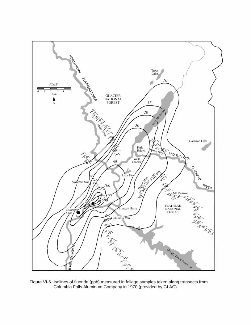
Figure VI-6. Isolines of fluoride (ppb) measured in foliage samples taken along transects from

Columbia Falls Aluminum Company in 1970 (provided by GLAC).

Figure VI-7. Permanent vegetation sampling locations in the southwestern portion of the park

(provided by GLAC).

4. Visibility

As part of the IMPROVE network, visual air quality in GLAC, Montana, has been monitored using

an aerosol sampler, transmissometer, and camera. The aerosol sampler has operated from

March 1988 through the present in the vicinity of the Glacier horse stables, approximately 2 miles

northwest of the GLAC west entrance. The transmissometer has been operating from March 1989

through the present and is located at the southern end of Lake McDonald, approximately 3 miles north

of the park’s west entrance. Two automatic 35mm camera systems were installed at the southern

shore of Lake McDonald in 1985. The primary camera system was located at the Apgar pump house,

viewing Lake McDonald and Garden Wall to the northeast from June 1985 through April 1995. A

second camera system was located on the southeast shoreline of Lake McDonald, from 1985 through

June 1991, viewing Teakettle Mountain and Lake McDonald to the southwest. Data from this

IMPROVE site have been summarized to characterize the full range of visibility conditions for the

March 1988 through February 1995 period, based on seasonal periods (Spring: March, April, and May;

Summer: June, July, and August; Autumn: September, October, and November; and Winter:

December, January, and February) and annual periods (March through February of the following year,

e.g., the annual period of 1994 includes March 1994 through February 1995). Complete descriptions

of visibility characterization, mechanisms of sources and visibility impacts, and IMPROVE monitoring

techniques and rationale are provided in the Introduction (Section I) of this document.

a. Aerosol Sampler Data - Particle Monitoring

IMPROVE aerosol samplers consist of four separate particle sampling modules that collect 24-

hour filter samples of the particles suspended in the air. The filters are then analyzed in the laboratory

to determine the mass concentration and chemical composition of the sampled particles. Particle data

can be used to provide a basis for inferring the probable sources of visibility impairment. Practical

considerations limit the data collection to two 24-hour samples per week. (Wednesday and Saturday

from midnight to midnight). Detailed descriptions of the aerosol sampler, laboratory analysis, and data

reduction procedures used can be found in the draft Standard Operating Procedures and Technical

Instructions for the IMPROVE Aerosol Sampling Network (U.C. Davis, 1996).

Aerosol sampler data are used to reconstruct the atmospheric extinction coefficient in

Mm-1 (inverse megameters) from experimentally determined extinction efficiencies of important

aerosol species. The extinction coefficient represents the ability of the atmosphere to scatter and

absorb light. Higher extinction coefficients signify lower visibility. A tabular and graphic summary of

average reconstructed extinction values by season and year for the March 1988 through February

1995 period are provided in Table VI-9 and Figure VI-8, respectively.

Table VI-9. Seasonal and annual average reconstructed extinction (Mm-1) and standard visual

range (km) at GLAC, March 1988 through February 1995.

Year

Spring

(Mar, Apr, May)

Summer

(Jun, Jul, Aug)

Autumn

(Sep, Oct, Nov)

Winter

(Dec, Jan, Feb)

Annual

(Mar-Feb)a

bext(Mm-1)

SVR (km)

bext(Mm-1)

SVR (km)

bext(Mm-1)

SVR (km)

bext(Mm-1)

SVR (km)

bext(Mm-1)

SVR (km)

1988 42.8 91 51.2 76 58.0 67 59.4 66 51.6 76 1989

48.9

80

49.3

79

59.7

66

71.2

55

56.5

69

1990 55.0

71

52.1

75

62.8

62

61.4

64

57.9

68

1991 49.4

79

51.0

77

74.5

53

73.4

53

61.3

64

1992 54.4

72

47.6

82

66.9

58

77.3

51

60.2

65

1993 43.6

90

43.4

90

72.9

54

67.2

58

56.1

70

1994 46.8

84

56.4

69

62.6

62

56.5

69

55.3

71

Meanb 48.7

57.7c 68c80 50.1 78 65.3 60 66.6 59

a Annual period data represent the mean of all data for each March through February annual

period. b Combined season data represent the mean of all seasonal means for each season of the March

1988 through February 1995 period. c Combined annual period data represent the mean of all combined season means.

Figure VI-8. Seasonal average reconstructed extinction (Mm-1) GLAC, March 1988 through February 1995.

Reconstructed extinction budgets generated from aerosol sampler data apportion the extinction at

GLAC to specific aerosol species (Figure VI-9). The species shown are Rayleigh, sulfate, nitrate,

organics, elemental (light absorbing) carbon, and coarse mass. The sum of these species account for

the majority of non-weather related extinctions. Extinction budgets are listed by season and by mean

of cleanest 20% of days, mean of the median 20% of days, and mean of the dirtiest 20% of days. The

"cleanest" and "dirtiest" signify lowest fine mass concentrations and highest fine mass concentrations

respectively, with "median" representing the 20% of days with fine mass concentrations in the middle

of the distribution. Each budget includes the corresponding extinction coefficient, visual range (in

kilometers), and deciview (dv).

Standard Visual Range (SVR) can be expressed as:

SVR (km) = 3,912 / (bext - bRay + 10)

where bext is the extinction coefficient expressed in inverse megameters (Mm-1), bRay is the site specific

Rayleigh values (elevation dependent), 10 is the Rayleigh coefficient used to normalize visual range,

and 3,912 is the constant derived from assuming a 2% contrast detection threshold.

The theoretical maximum SVR is 391 km. Note that bext and SVR are inversely related: for example,

as the air becomes cleaner, bext values decrease and SVR values increase.

Deciview is defined as:

dv = 10 ln(bext/10Mm-1)

where bext is the extinction coefficient expressed in inverse megameters (Mm-1). A one dv change is

approximately a 10% change in bext, which is a small but perceptible scenic change under many

circumstances. The deciview scale is near zero (0) for a Rayleigh atmosphere and increases as

visibility is degraded. The segment at the bottom of each stacked bar represents Rayleigh scattering,

which is assumed to be a constant 10 Mm-1 at all sites during all seasons. Rayleigh scattering is the

natural scattering of light by atmospheric gases. Higher fractions of extinction due to Rayleigh

scattering indicate cleaner conditions.

The reconstructed extinction data are used as background conditions to run plume and regional

haze models. These data are also used in the analysis of visibility trends and conditions. The

measured extinction data are used to verify the calculated reconstructed extinction and can also be

used to run plume and regional haze models and to analyze trends and conditions. Because of the

larger spatial and temporal range of the aerosol data, reconstructed extinction data are preferred.

Figure VI-9. Reconstructed extinction budgets for GLAC, Montana, March 1988 - February 1995.

b. Transmissometer Data - Optical Monitoring

The transmissometer system consists of two individually-housed primary components: a

transmitter (light source) and a receiver (detector). The light extinction coefficient (bext) at any time can

be calculated based on the intensity of light emitted from the source and the amount of light measured

by the receiver (along with the path length between the two). Transmissometers provide continuous,

hourly bext measurements. Meteorological or optical interference factors (such as clouds, rain, or a

dirty optical surface) can affect transmissometer measurements. Collected data that may be affected

by such interferences are flagged invalid, “filtered.” Seasonal and annual data summaries are typically

presented both with and without weather-influenced data. Detailed descriptions of the

transmissometer system and data reduction and validation procedures used can be found in Standard

Operating Procedures and Technical Instructions for Optec LPV-2 Transmissometer Systems (ARS,

1993 and 1994).

Table VI-10 provides a tabular summary of the “filtered” seasonal and combined period arithmetic

mean extinction values for the March 1989 through February 1995 period. Table VI-11 provides a

tabular summary of the "filtered" seasonal and combined period 10% (clean) cumulative frequency

values. Data are represented according to the following conditions:

• No data are reported for seasons when the percentage of valid hourly averages (including weather) compared to total possible hourly averages, was less than 50%.

• Annual data represent the mean of all valid seasonal bext values for each March through

February annual period. No data are reported for years that had one or more invalid seasons.

• Combined season data represent the mean of all valid seasonal bext values for each

season (spring, summer, autumn, winter) of the March 1989 through February 1995 period.

• Combined annual period data represent the unweighted mean of all combined seasonal bext values.

Figure VI-10 provides a graphic representation of the "filtered" annual mean, median, and

cumulative frequency values (5th, 10th, 25th, 75th, 90th, and 95th percentiles). No data are reported

for annual periods with one or more invalid seasons.

When comparing reconstructed (aerosol) extinction, Table VI-10 with measured

(transmissometer) extinction, Table VI-11, the following differences/similarities should be considered:

• Data Collection - Reconstructed extinction measurements represent 24-hour samples collected twice per week. Transmissometer extinction estimates represent continuous measurements summarized as hourly means, 24 hours per day, seven days per week.

• Point versus Path Measurements - Reconstructed extinction represents an indirect measure of

extinction at one point source. The transmissometer directly measures the irradiance of light (which calculated gives a direct measure of extinction) over a finite atmospheric path.

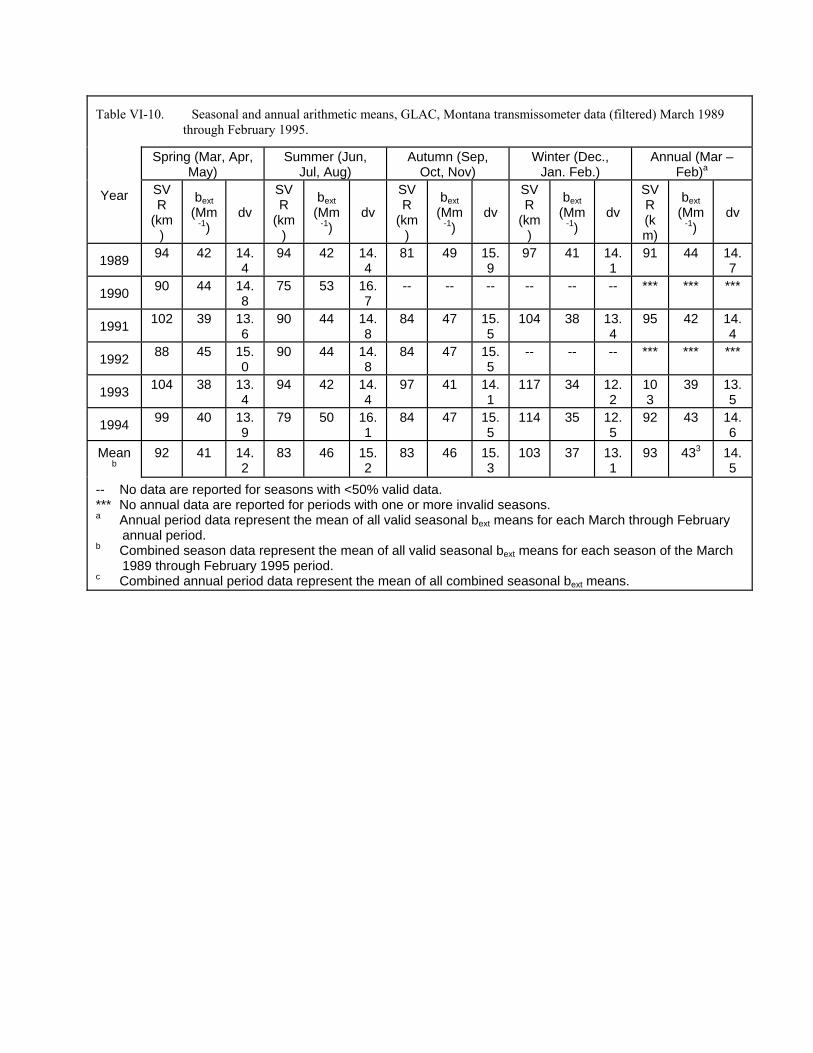
Table VI-10. Seasonal and annual arithmetic means, GLAC, Montana transmissometer data (filtered) March 1989

through February 1995. Spring (Mar, Apr,

May)

Summer (Jun,

Jul, Aug)

Autumn (Sep,

Oct, Nov)

Winter (Dec.,

Jan. Feb.)

Annual (Mar –

Feb)a

Year

SVR

(km)

bext

(Mm-1)

dv

SVR

(km)

bext

(Mm-1)

dv

SVR

(km)

bext

(Mm-1)

dv

SVR

(km)

bext

(Mm-1)

dv

SVR (k

) m

bext

(Mm-1)

dv

1989

94

42

14.4

94

42

14.4

81

49

15.9

97

41

14.1

91

44

14.7

1990

90

44

14.8

75

53

16.7

--

--

--

--

--

--

***

***

***

1991

102

39

13.6

90

44

14.8

84

47

15.5

104

38

13.4

95

42

14.4

1992

88

45

15.0

90

44

14.8

84

47

15.5

--

--

--

***

***

***

1993

104

38

13.4

94

42

14.4

97

41

14.1

117

34

12.2

103

39

13.5

1994

99

40

13.9

79

50

16.1

84

47

15.5

114

35

12.5

92

43

14.6

Meanb

92

41

14.2

83

46

15.2

83

46

15.3

103

37

13.1

93

433

14.5

-- No data are reported for seasons with <50% valid data. *** No annual data are reported for periods with one or more invalid seasons. a Annual period data represent the mean of all valid seasonal bext means for each March through February

annual period. b Combined season data represent the mean of all valid seasonal bext means for each season of the March

1989 through February 1995 period. c Combined annual period data represent the mean of all combined seasonal bext means.

Table VI-11. Seasonal and annual 10% (Clean) cumulative frequency statistics GLAC, transmissometer data

(filtered) March 1989 through February 1995.

Spring (Mar, Apr, May)

Summer

(Jun, Jul, Aug)

Autumn

(Sep, Oct, Nov)

Winter

(Dec., Jan, Feb)

Annual

(Mar – Feb)a Yea

r

SVR

(km)

bext

(Mm-1)

dv

SVR

(km)

bext

(Mm-1)

dv

SVR

(km)

bext

(Mm-1)

dv

SVR

(km)

bext

(Mm-1)

dv

SVR (km)

bext

(Mm-1)

dv

1989

160

25

9.2

143

28

10.3

174

23

8.3

182

22

7.9

164

25

9.0

1990

143

28

10.3

133

30

11.0

--

--

--

--

--

--

***

***

***

1991

167

24

8.8

138

29

10.6

160

25

9.2

182

22

7.9

161

25

9.2

1992

138

29

10.6

143

28

10.3

138

29

10.6

--

--

--

***

***

***

1993

160

25

9.2

154

26

9.6

191

21

7.4

191

21

7.4

173

23

8.4

1994

167

24

8.8

138

29

10.6

160

25

9.2

148

27

9.9

153

26

9.7

Meanb

145

26

9.5

133

28

10.4

253 9.3 152 25 9.0 162 23 8.3 15

8 -- No data are reported for seasons with <50% valid data. *** No annual data are reported for periods with one or more invalid seasons. a Annual data represent the mean of all valid seasonal bext values for each March through

February annual period. b Combined season data represent the mean of all valid seasonal bext values for each season of

the March 1989 through February 1995 period. c Combined annual period data represent the mean of all combined seasonal bext values.

Figure VI-10. Annual arithmetic mean and cumulative frequency statistics, GLAC, Montana,

transmissometer data (filtered).

• Relative Humidity (RH) Cutoff - Daily average reconstructed measurements are flagged as invalid when the daily average RH is greater than 98%. Hourly average transmissometer measurements are typically flagged invalid when the hourly average RH is greater than 90%. These flagging differences often result in data sets that do not reflect the same period of time, or misinterpret short-term meteorological conditions.

Note: All March 1993 through February 1995 GLAC transmissometer data were processed

using a site-specific relative humidity upper limit of 95%. The transmissometer site path

at GLAC views across Lake McDonald and is relatively near the lake’s surface. The site-

specific RH limit was changed in the Spring of 1993 to reduce the number of hourly

extinction values invalidated due to the higher relative humidity values associated with

the site.

c. Camera Data - View Monitoring

Two automatic 35mm camera systems operated from the southern shoreline of Lake McDonald

in GLAC. The primary system took photographs of Lake McDonald and Garden Wall three times per

day from June 1985 through April 1995. A second camera system took photographs of Lake

McDonald and Teakettle Mountain three times per day from June 1985 through June 1991.

View monitoring slides document visual conditions and are an effective tool for interpreting the

visual effects of measured optical and aerosol parameters or presenting monitoring program goals,

objectives, and results to decision-makers and the public. The Garden Wall vista photographs

presented in Figure VI-11 were chosen to provide a feel for the range of visibility conditions possible

and to help relate the extinction/SVR/haziness data to the visual sense.

Figure VI-11 Photographs illustrating visibility conditions at Glacier National Park.

d. Visibility Summary

Data from other IMPROVE visibility sites around the country have been presented graphically

(Figure I-1 and Figure I-2) so that visual air quality in the Rocky Mountains and Northern Great

Plains regions can be understood in perspective. Figure VI-8 and Table VI-10 have been provided

to summarize GLAC visual air quality during the March 1988 through February 1995 period.

Seasonal extinction data should be reviewed with caution given the transmissometer’s close

proximity to Lake McDonald and higher than normal relative humidity values associated with the

data. Long-term trends fall into three categories: increases, decreases, and variable. Given the

visibility sites summarized for this report, the majority of data show little change or trends.

Non-Rayleigh atmospheric light extinction at GLAC, like many rural western areas, is largely

due to sulfate, organics, and soil. Historically, visibility varies with patterns in weather, winds (and

the effects of winds on coarse particles) and smoke from fires. No information is available on how

the distribution of visibility conditions at present differs from the profile under "natural" conditions, but

the cleanest 20% of the days probably approach natural conditions (GCVTC, 1996). Smoke from

frequent fires is suspected to have reduced pre-settlement visibility below current levels during some

summer months.

The IMPROVE aerosol monitoring network, established in March 1988, consists of sites

instrumented with aerosol sampling modules A through D. Many of the IMPROVE sites are

successors to sites where aerosol monitoring with stacked filter units (SFU) was carried out as early

as 1979. SFU data were collected at GLAC from October 1982 through May 1986. Although some

seasonal trends in absorption were observed for GLAC, no long-term trends were apparent in the

1982 through 1986 SFU data or the 1989 through 1994 site-specific or regional data presented in

this report.

D. AIR QUALITY RELATED VALUES

1. Lakes and Streams

Sensitive fish species in the park include both native and non-native salmonids. Native western

trout are sensitive to short-term increases in acidity. For example, eggs, alevins, and swim-up larvae

of cutthroat trout were shown to have significantly higher mortality at pH 4.5 than at pH 6.5. Mortality

was also higher at pH 5.0, but only statistically higher for eggs (Woodward et al. 1989).

It is unlikely that aquatic biota in GLAC have experienced adverse impacts to date from acidic

deposition. This is because N and S deposition are low, the available lake water chemistry data do

not suggest chronic acidification, and most sampled lakes appear to be relatively insensitive to

acidification at any foreseeable levels of acidic deposition. However, in view of the apparent

sensitivity of at least some waters in the park to future increases in acidic deposition and the

outstanding quality of aquatic resources in GLAC, aquatic biota constitute important AQRVs within

GLAC.

2. Terrestrial Vegetation is the resource which is most sensitive to ozone and SO2, and several tree species

have been identified as potential bioindicators (see below). While ozone levels in the park have not

exceeded the NAAQS, future increases in ozone might damage sensitive plant species. Potential

impacts of fluoride are a source of concern due to emissions from the Columbia Falls Aluminum

Company plant, because fluoride injury in conifer needles causes tip burn, reduced diameter growth

and abscission of older foliage (Shaw et al. 1951). However, little is known about the sensitivity of

native plant species to fluoride.

In addition to vegetation, insects, mammals, and other organisms may be impacted by fluoride.

It is stored in plant tissues including leaves, stems, cambium and bark, and is passed on to

numerous organisms which feed on these tissues. Studies in the GLAC region of fluoride content

from foliage- and cambial-feeding, predaceous, and pollinating insects found the highest

concentrations of fluorides (400 ppb dry weight) in bumblebees (Carlson and Dewey 1971).

Predaceous species had fluoride levels ranging from 60 to 170 ppb dry weight and foliage feeders

ranged from 21 to 48 ppb dry weight. High levels of fluoride have also been found in other

organisms. Bone tissue from grouse, chipmunks, deer mice and deer in the GLAC region had

between 4 and 6 times more fluoride than control animals (Gordon 1972, 1974). It is unknown what

levels of fluoride will cause fluorosis, a toxic response in animals.

Ponderosa pine is not widespread in GLAC, although stands on the western edge of the park

are suitable for establishing long-term monitoring plots for ozone. Of the hardwood species present

at GLAC, quaking aspen is the most sensitive to ozone. Aspen grows at various locations in riparian

ecosystems and in fire- or avalanche-disturbed areas in the park. Black cottonwood (Populus

trichocarpa var. balsamifera), another potential bioindicator for ozone (Woo 1996), has symptoms

similar to those of aspen. However, it is generally regarded as less sensitive to ozone than aspen.

Neither of these hardwood species has the clarity of ozone symptomatology found in ponderosa

pine.

Aspen is also considered to be sensitive to SO2 and may be the best sensitive receptor for this

gaseous pollutant. Injury is similar to that normally found for ozone (stippling, followed by bifacial

necrosis), although SO2 - induced injury rapidly bleaches to a light tan color, whereas ozone injury

remains dark (Karnosky 1976). Caution should be used in distinguishing ozone injury from SO2

injury.

Most fluoride sensitivity studies have focused on ponderosa pine (both varieties). Early

accounts of fluoride injury in ponderosa pine were reported near Kaiser Aluminum Company in

Mead, Washington, with symptoms of retarded stem-diameter growth and foliar necrosis (Shaw et al

1951, Lynch 1951, Adams et al 1956). A study conducted in the vicinity of Harvey Aluminum

Company in The Dalles, Oregon, found foliar injury in ponderosa pine to be attributed to elevated

fluoride and not fungal, insect or pathogen agents (Compton et al. 1961). Later studies done in

Flathead National Forest and GLAC in 1974 indicated that western white pine appeared to be the

most sensitive conifer to fluoride (Carlson and Dewey 1971); ponderosa pine, lodgepole pine, and

Douglas-fir were moderately sensitive, and Engelmann spruce, western redcedar, and subalpine fir

were most tolerant. Of the shrub species observed, Carlson and Dewey found that chokecherry

(Prunus virginiana) and serviceberry (Amelanchier alnifolia) appeared more sensitive to fluoride than

other shrubs. False-lily-of-the-valley (Maianthemum dillatatum) and disporum (Disporum hookeri)

were the most sensitive of the herbaceous species studied. These are general classifications based

on field data and observations, not on data from laboratory studies.

A species list of native plants is available in the NPFlora database. Table VI-12 summarizes

vascular plant species of GLAC with known sensitivity to ozone, SO2 and NOx. This table is based

on a variety of sources from the published literature and other information. It should be noted that

the various sources used a wide range of field and experimental approaches to determine pollutant

pathology, and that sensitivity ratings are general estimates based on published information and our

expert opinion. While it will not be possible for park staff to collect data on all the species indicated

in Table VI-12, the list can be used by park managers as a guide for identifying visible symptoms.

Of the many plant species in GLAC, it is likely that there are many other species which have high

sensitivity to air pollution, but we currently have no information about them.

Table VI-12. Plant species of GLAC with known sensitivities to sulfur dioxide, ozone

and nitrogen oxides. (H=high, M=medium, L=low, blank=unknown). (Sources: Esserlieu and Olson 1986, Bunin 1990, Peterson et al. 1993, National Park Service 1994, Electric Power Research Institute 1995, Binkley et al. 1996, Brace and Peterson 1996)

Species Name

SO2 Sensitivity

O3 Sensitivity

NOx Sensitivity

Abies lasiocarpa L L Acer glabrum H Acer glabrum douglasii M Achillea millefolium L Agastache urticifolia M Agoseris glauca M Amaranthus retroflexus M Ambrosia psilostachya L Amelanchier alnifolia H M Arctostaphylos UVa-ursi L L Artemisia ludoviciana M Artemisia tridentata M L Betula occidentalis M Table VI-12. Continued.

Species Name SO2 Sensitivity

O3 Sensitivity

NOx Sensitivity

Betula papyrifera H H Betula papyrifera commutata H Betula papyrifera subcordata H Bromus carinatus L Bromus tectorum M Carex siccata L Cassiope mertensiana L Ceanothus sanguineus M Ceanothus velutinus L Ceanothus velutinus laevigatus L Chenopodium fremontii L Cirsium arvense L Cirsium undulatum M Clematis ligusticifolia M Collomia linearis L Convolvulus arvensis H Cornus stolonifera M L Crataegus columbiana M Crataegus douglasii L Descurainia pinnata L Erigeron peregrinus L Fragaria virginiana H Galium bifolium L Gayophytum racemosum L Gentiana amarella M Geranium richardsonii M M

Hackelia floribunda L Hedysarum boreale M Helianthus anuus H L Holodiscus discolor H H Hymenoxys richardsonii L Juniperus communis L Juniperus scopulorum L Larix lyalii H Larix occidentalis H Lonicera involucrata L H Medicago sativa M Mimulus guttatus L Osmorhiza occidentalis L Pachistima myrsinites L Phacelia heterophylla L Philadelphys lewisii H Phyllodoce empetriformis L Picea engelmannii M L Picea glauca

M

L

Pinus contorta M M H Pinus contorta latifolia H M Pinus flexilis L Pinus monticola M M Table VI-12. Continued.

Species Name SO2 Sensitivity

O3 Sensitivity

NOx Sensitivity

Pinus ponderosa M H H Poa annua H L Poa pratensis L Polygonum douglasii L Populus balsamifera trichocarpa M H Populus tremuloides H H Populus trichocarpa M H Potentilla fruticosa L Prunus emarginata H Prunus virginiana M H Pseudotsuga menziesii M L H Pseudotsuga menziesii glauca M L Ribes lacustre M Ribes viscosissimum M Rosa woodsii M L Rubus idaeus H Rubus parviflorus H M Rumex crispus L Salix scouleriana M Sambucus racemosa L Shepherdia canadensis L Sorbus scopulina M Sorbus sitchensis H Symphoricarpos albus H

Taraxacum officinale L Taxus brevifolia L Thuja plicata L Tragopogon dubius M Trifolium pratense L Trifolium repens H Trisetum spicatum M Tsuga heterophylla

M

Tsuga mertensiana H Urtica gracilis L Vaccinium membranaceum M Vicia americana L Viola adunca L

An inventory of lichen species with known sensitivity to ozone and SO2 is summarized in Table

VI-13. As in Table VI-12, this table is based on a variety of sources from the published literature and

other information. It should be noted that diagnostic symptoms of air pollutant injury to lichens are

difficult to identify, and that some species have reduced productivity or even mortality without

exhibiting visible symptoms (Nash and Wirth 1988). One of the best sources of background

information and guidelines for addressing the use of lichens as sensitive receptors of air pollution is

Stolte et al. (1993). The inventory of GLAC lichen species performed by DeBolt and McCune (1993)

provides a good baseline for further assessment of potential impacts of air pollution.

Table VI-13. Lichen species of GLAC with known sensitivity to SO2 and ozone.

(H=high, M=medium, L=low, blank=unknown) (Sources: Peterson et al. 1993, Electric Power Research Institute 1995, Binkley et al. 1996).

Species

SO2 sensitivity

Ozone sensitivity

Acarospora chlorophana H Alectoria sarmentosa H Bryoria abbreviata H Bryoria capillaris H Bryoria fremontii H Bryoria fuscescens M Bryoria glabra M H Bryoria implexa H Bryoria oregana H Calicium viride L-M H Caloplaca flavorubescens H Caloplaca holocarpa M Candelariella vitellina M Cetraria canadensis H Cetraria cucullata M Cetraria islandica M H Cetraria nivalis M Cetraria pinasrtri M

Chrysothrix candellaris L Cladonia coniocraea M Cladonia fimbriata M-H Cladonia gracilis L-M Coeocaulon muricatum L-M Collema tenax M Evernia prunastri L-M H Hypocenomyces scalaris M Hypogymnia imshaugii L-M L-M Hypogymnia physodes L-M Lecanora carpinea M Lecanora dispersa L Lecanora hageni L-M Lecanora muralis M Lecidea atrobrunnea L Letharia columbiana L L-M Letharia vulpina L L-M Lobaria pulmonaria H L-M Melanelia elegantula L Melanelia exasperatula M Melanelia subaurifera H Melanelia subolivacea L-M Mycoblastus sanguinarius L-M Parmelia saxatilis M L Parmelia sulcata L-M M-H Parmeliopsis ambigua M Parmeliopsis hyperopta M Table 13. Continued Species

SO2 sensitivity

Ozone sensitivity

Peltigera aphthosa M H Peltigera canina L H Peltigera collina H Peltigera didactyla H Peltigera refuscens M-H Phaeophyscia orbicularis M H Phaeophyscia sciastra H Physcia adscendens M Physcia aipolia M Physcia caesia M Physcia dubia M Physcia stellaris L-M Physcia tenella M L Physconia detersa M-H L Platismatia glauca M H Pseudephebe minuscula M Pseudephebe pubescens M Ramalina obtusata M Rhizocarpon geographicum L Rhizoplaca chrysoleuca H Rhizoplaca melanophthalma H

Umbilicaria polyphylla L-M Usnea subfloridana M-H Xanthoparmelia cumberlandia H Xanthoria candelaria M-H H Xanthoria elegans M Xanthoria fallax M-H L Xanthoria polycarpa M L

A fluoride injury index was developed by Carlson and Dewey (1971) from foliage collected in

Flathead National Forest and GLAC (Table VI-14). Their classification was based on visual injury

found in lodgepole pine, western white pine, whitebark pine, ponderosa pine and Douglas-fir

between the 30 and 100 ppb dry weight isolines (Figure VI-6).

Table VI-14. Classification of visual injury of fluoride in

conifers. (Source: Carlson and Dewey 1971)

Class

Fluoride Concentration (ppb) Non-injured < 60 Light 61-500 Moderate 501-999 Severe > 1000

E. RESEARCH AND MONITORING NEEDS

1. Deposition and Gases

We recommend continued gas and deposition monitoring at the GLAC Fire Weather Station

(Apgar). This will provide important long-term data for continued evaluation of potential resource

effects. This is needed in view of the sensitivity of some resources and the outstanding quality of

aquatic resources in the park, including the importance of the native cutthroat trout gene pool.

Little is known of the present threats of ozone, SO2, and NO2 on native vegetation in GLAC.

Ozone data are currently collected at GLAC from a continuous electronic analyzer near park

headquarters. An additional analyzer installed seasonally (for summer months) at a high elevation

site (e.g., Logan Pass Visitors Center) for three consecutive years would provide valuable

information on the diurnal pattern and elevational differences of ozone exposure within the park.

Studies of ozone profiles done in other mountainous areas including the Swiss Alps (Sandroni et al.

1994), the Sierra Nevada and the Cascade Mountains (Brace and Peterson 1996, 1998) have shown

that topography and elevation can influence the diurnal exposure. Low-elevation sites have diurnal

profiles characterized by low ozone levels during the nighttime and early morning hours, maximum

levels during the mid or late afternoon, and low levels again in the evening. High-elevation sites

typically have lower maximum ozone concentrations than low elevation sites, but ozone remains

elevated during the morning and nighttime hours. Plant species at higher elevations may be at risk

from exposure to elevated levels of ambient ozone during the morning hours when they are

physiologically active.

In addition to maintaining the permanent continuous ozone analyzer in the Apgar area, we

believe that it would be useful to install a network of passive samplers to obtain data on spatial

variability of weekly ozone exposures in different areas of the park. Two transects should suffice,

placed along elevational gradients and sampled weekly for two months each summer for three

years. Transects should be located in areas with maximum airflow and downwind from potential

precursor sources (VOC and NOx). An additional transect could be placed in an area considered

least exposed to transported ozone and precursors.

Continued SO2 monitoring is important, considering the proximity of Columbia Falls Aluminum

Company, the largest point source of SO2 in the area. In addition, continued fluoride monitoring will

contribute valuable data on fluoride deposition in GLAC.

2. Aquatic Systems

Ellis et al. (1992) recommended continuous monitoring of three lakes in GLAC, using a mass

balance approach to allow interpretation of the impact of incremental increases in acidic deposition

on lake buffering capacity. This would include quantification of solute fluxes into and out of the

alpine lakes, including measurements of discharge, snow pack surveys, and air temperature and

humidity data (for evaporation estimation). They recommended depth profiling of key variables at

least three times per year, once during winter ice cover, immediately following surface ice melt, and

during late summer. Cobalt, Upper Dutch, and Medicine Grizzly were judged to be easily accessed

and representative of the range of conditions found in the alpine lakes. These were the preferred

candidate lakes for continuous monitoring. Ellis et al. (1992) also recommended monitoring other

lakes on a five-year interval schedule.

It is our judgment that none of the lakes studied by Ellis et al. (1992) are sufficiently acid-

sensitive as to warrant the intensive monitoring effort proposed. In our view, only Cobalt Lake is

sufficiently dilute (sensitive) to be acidified by air pollutants to ANC approaching zero on an episodic

basis in the foreseeable future. None of the lakes are at risk for chronic acidification to ANC < 0.

Our judgement is based on the observations that 1) both ANC values and CB minus (SOB 42- + NO3

-)

values are consistently greater than about 70 to 80 µeq/L, and 2) the sum of (SO42- + NO3

-)

concentrations in the lowest ANC lakes are less than 20 µeq/L and generally closer to about 10

µeq/L. Thus, the concentration of (SO42- + NO3

-) in these lakes would need to increase by more

than a factor of four, perhaps by a factor of ten, before such lakes would become chronically acidic

(ANC < 0) (cf., Husar et al. 1991, Sullivan and Eilers 1994). Cobalt Lake is a good candidate for

continued chemical and ecological monitoring, however. We recommend water quality sampling

twice per year, immediately after ice-out and during July or August. We do not advocate hydrologic

or additional deposition monitoring for this lake at this time. Snyder Lake is also a good candidate

for continued chemical and ecological monitoring because it is located on the west side of the

Continental Divide in the central portion of the park. It is exposed to air masses that are transported

to the park from the southwest. Even though it is located in a headwater area, the elevation is fairly

low (1,597 m), which is likely a major factor responsible for the lake having fish present (Ellis et al.

1992). However, based on its measured lakewater chemistry, Snyder Lake is relatively insensitive to

acidic deposition effects. The average sum of base cation concentrations measured by Ellis et al.

(1992) was 152 μeq/L and average alkalinity at about the same level. Snyder Lake would not be

expected to acidify due to acidic deposition in the future. Average SO42- concentration was only 13

μeq/L, suggesting that most SO42- in the lake is of atmospheric origin. Nevertheless, monitoring this

lake will provide indication of changes in the contributions of SO42- and NO3

- to lakewater during

snowmelt and on a chronic basis. It is relatively easily accessed and has the added benefit of a

biological receptor in the form of native cutthroat trout. If, for example, lakewater concentrations of

SO42- or NO3

- were to increase dramatically (perhaps three-fold) in the future, then additional

biological monitoring would be appropriate.

Ellis et al. (1992) did not sample lakes in the northwestern portion of the park. The closest to

that area of the park was Gyrfalcon Lake. Based on examination of topographic maps, Gyrfalcon

Lake appears to receive substantial glacial meltwater input. This would account for its relatively high

concentrations of base cations and alkalinity. Many lakes situated in areas expected to be highly

sensitive to acidic deposition within this part of the park (i.e., cirque lakes below steep ridges) are, in

fact, fed by glaciers. Due to the high degree of buffering generally found in glacial meltwater, none

of these lakes would be expected to be highly sensitive to the effects of acidic deposition. There are

a few appropriate candidate lakes for high acid-sensitivity, however, in the northwestern portion of

the park. These include Long Bow Lake (and its unnamed upstream tributary lake) and Pocket

Lake. Each is located on the west side of the Continental Divide in a headwater area and apparently

without substantial glacial meltwater contributions. The logistics of sampling each of these lakes

may be difficult. If feasible, we recommend sampling each lake once for water quality, and if one is

found to be highly sensitive, adding it to the list of recommended long-term monitoring lakes.

3. Terrestrial Systems

Additional studies are needed to evaluate the impact of ambient fluoride on terrestrial

ecosystems in GLAC. While adequate data exist on plant biomass content of fluoride in several

plant species commonly found in GLAC, more detailed studies on physiological responses to

ambient fluoride levels need to be developed. Plant injury symptoms and changes in growth and

phenology need to be identified and documented through controlled chamber or greenhouse studies.

If park managers want to accurately evaluate the impact of fluoride on vegetation, the following

steps are recommended:

· Grasses, shrubs, and herbaceous species should be identified, analyzed, and reported

separately instead of using the collective category "elk forage". This will provide more scientific and ecological value to the vegetation data.

· Controlled-fumigation studies should be included in the monitoring plan to elicit physiological

response data on 4-5 tree, shrub and herbaceous species. Such studies should include measurements of changes in stem, root and leaf/needle growth, respiration, and foliar health (necrosis, chlorosis, tip burn) under a variety of exposure profiles. Exposures should include profiles of ambient, moderate, and high fluoride levels within a range of 20 - 1,000 ppbv, to reflect levels currently measured near Columbia Falls and the Flathead region.

· A complete photoguide of fluoride-induced injury in foliage can be compiled from symptoms

obtained in the controlled fumigation studies. Consultation with a pathologist and/or entomologist is recommended to confirm that foliar injury is caused by fluoride, not by pathogens, nutrient deficiency, insects, fungal agents, or other factors.

· Controlled-fumigation studies should be considered for 4-5 common lichen species.

Common foliose or species with large thallus surface area should be selected. Photographs of thallus injury can be compiled in a field-guide.

Currently, the threats to GLAC terrestrial resources from ozone and SO2 are not sufficiently

urgent to warrant monitoring of sensitive species. However, if pollution levels increase in the future,

monitoring of terrestrial resources can be considered. Three levels of monitoring associated with

increasing amounts of effort and expense are detailed in Appendix A. These monitoring activities

are based on methods and protocols developed by the USDA Forest Service and NPS. Species and

locations recommended for monitoring are listed below.

If monitoring for potential impacts of ozone and SO2 is implemented, we recommend placing

plots at three locations in the western and southwestern portion of GLAC, where airflow from

Kalispell and Columbia Falls first reaches the park: (1) ponderosa pine in meadows west of

headquarters and Apgar, (2) quaking aspen at lower to mid-elevation where reasonably continuous

stands exist, and (3) subalpine fir at higher elevation.

Additional plots could be located along the Going-to-the-Sun Road from Apgar to Logan Pass.

This valley is where maximum levels of ozone and other pollutants transported by prevailing winds

might be expected. All sites should be accessible from the road. Locations of these plots can be

changed to other sites in GLAC if ambient air quality data indicate that other areas have a higher risk

of pollutant effects.

If lichens are included in a monitoring effort, they should be monitored on the south and west

side of GLAC, as described in Appendix A. Three of the monitoring sites should be co-located with

the tree monitoring plots in GLAC as described above. Additional lichen monitoring sites could be

located in the alpine zone and along the elevational gradients described for tree monitoring above.

Additional tree plots could be located along elevational transects that evaluate other conifer

species, such as Engelmann spruce, lodgepole pine, Douglas-fir, and whitebark pine. It is unknown

how many of these species will be found along each transect, but it is recommended that at least

two additional species be identified on each transect.

4. Visibility

IMPROVE aerosol and optical monitoring continues today at GLAC. Ongoing and future

monitoring is necessary to identify local source impacts. Additional data and in-depth modeling and

analysis are required to further evaluate historical trends and future projections of impact from

existing and future sources. For example, back trajectory analysis and spatial/temporal pattern

analysis of episodes are recommended to determine the source region contributions to elevated

aerosol concentrations. Future research is also recommended to minimize the uncertainty in

estimates of how various aerosol species affect visibility.

To enhance monitoring at GLAC, a monitoring site (particle and optical monitoring) could be

established on the east side of the park. Dramatic differences in elevation can produce significantly

different visibility conditions. Visibility monitoring sites at different elevations would therefore be

desirable. This additional monitoring would help to better assess visibility impairment at the park.