• /

r-b

m •

CSDL-T-_8

STEERING LAW DESIGN FOR REDUNDANT SINGLEGIMBAL CONTROL MOMENT GYRO SYSTEMS

by

Nee Sarkb Bedrcmian

Augmt 1987

Vhe Cl.arles Stark Draper Laboratory, Inc.5 Techr, o_ogy Square

C_mbrid_';e, Massachusetts 02139

li|¢Uli[Alil SIN_LI_ (_I,_'=iL (-(_1_(L _(P._NT t;YBC

5152BR5 _.5. _(:si-', - P.assacbu_ettE Inst. ot

lechncloqy. (C'._,_._'_ ((bdzie-_ Stalk) haL.) Unclas

ltll F Jvaz;" 1_2_ r.(. A_7/_ JlC1 _CI, 1;b GJ/3_ ccgt_._l

®

https://ntrs.nasa.gov/search.jsp?R=19870019449 2018-06-12T18:21:43+00:00Z

STEERING LAW DESIGN FOR REDUNDANT SINGLE GISIBALCONTROL MOMENT GYRO SYSTEMS

by

NAZARETH SARKIS BEDROSSIAN

BSME University of Florida(1984)

SUBMITTED IN PARTIAL FULFILLMENT

OF THE REQUIREMENTS FOR THEDEGREE OF

MASTER OF SCIENCE

iN MECHANICAL ENGINEERING

at the

MASSACHUSETTS INSTITUTE OF TECHNOLOGY

August 1987

c Charles Stark Draper Laboratory inc., 1987

Signature of Author

Certified by

Certified by _

/

/O'U O'E_AJ" ./I//_,,._ /1 _:

" Department of" Mechanical EngineeringAugust 7, 1987

ProCessor Derek Rowell

Thesis Supervisor

Accepted byProfessor Ain A. Sonin

Chairman, Departmental Graduate Committe

STEERING LAW DESIGN FOR REDUNDANT SINGLE GIMBALCONTROL MOMENT GYRO SYSTEMS

by

NAZARETH SARKIS BEDROSSIAN

Submitted to the Department of Mechanical Engineeringon August 7, 1987 in partial fulfillment of

the requirements For the Degree ofMaster of Science in Mechanical Engineering

ABSTRACT

In this thesis, the correspondence between robotic manipulators and single gimba!Control Moment Gyro (CMG) systems was exploited to aid in the understanding anddesign of single gimbal CMG Steering laws. A test for null motion near a singularCMG configuration was derived which is able to distinguish between cscapable andunescapable singular states. Detailed analysis of the Jacobian matrix null-space wasperformed and results were used to develop and test a variety of single gimbal CMGsteering laws.

Computer simulations showed that all existing singularity avoidance methods areunable to avoid Elli,_tic internal singularities. A new null motion algorithm using theMoore-Penrose pseudoinverse, however, was shown by simulation to avoid Elliptictype singularities under certain conditions. The SR-inverse, with appropriate nullmotion was proposed as a general approach to singularity avoidance, because of itsability to avoid singularities through limited introduction of torque error. Simulationresults confirmed the superior performance of this method compared to the other avail-able and proposed pseudoinverse-based Steering laws.

Thesis Supervisor: Dr. Derek RowellProfessor of Mechanical Engineering

Technical Supervisor: Edward V. BergmannSection Chief, Charles Stark Draper Laboratory

I

ACKNOWLEDGEM ENTS

First and foremost, I would like to thank the Charles Stark Draper Laboratory for

affording me the opportunity to continue my graduate education at MIT, and provid-

ing the excellent environment, abundant resources, and generous financial support,

which have made this thesis much easier. I am especially gratefull to Dave Redding for

having enough faith in me, and for providing guidance" and advice. Ed Bergmann

deserves special mention for allowing me the freedom to explore this thesis area. I

would also like to thank Prof. Rowcll for overseeing this thesis.

This research benefited enormously from discussions with Joe Paradiso. He was

always available to listen and provide valuable suggestions about the subject matter.

He also deserves my sincere gratitude for painstakingly reviewing this thesis from cover

to cover, and providing constructive criticism. I would like to thank my officemate

Brent Appleby, for providing a sounding board for my ideas as well as valuable advise,

and assisting with the development of the simulation package. I would also like to

thank Marty Matuski, Neil Adams, Phil Hattis, Greg Barton and his fan, Greg Chami-

toff, and John Dzielski for helpful discussions. Also Bob Roucher and the consulting

staff deserve special praise for their invaluable assistance in preparing this document.

l would like to thank my parents for their love and guidance throughout the years.

Finally, I can never thank enough my wife Melinda, who has supported me with such

remarkable patience and sensitivity.

This report was prepared at The Charles Stark Draper l.aboratory, Inc. under con-

tract NAS9-17560 with the National Aeronautics and Space Administration.

Publication of this report does not constitute approval by the Charles Stark Draper

Laboratory or NASA of the findings or conclusions contained herein. It is published

solely ['or the excha nge of ideas.

Li

TABLE OF CONTENTS

CHAPTER Page

I. INTRODUCTION ............................................ 10

2. SINGLE GIMBAL (SG) CONTROL MOMENT GYRO (CMG) FUNDA-

MENTALS .................................................. 13

2.1 Characteristics of SG sytcms ................................ 13

2.2 Principle of Operation ....................... : .............. 14

2.3 Mechanical Analog ........................................ 16

2.4 Torque and ,Non-Torque Producing Motions ..................... 19

2.5 Examples OfSG CMG Systern And Planar Manipulator ............ 23

2.5.1

2.5.2

2.5.3

4-Pyramid Mounted SG CMG System ....................... 23

Null-Space Of Jacobian Matrix And The Generalized Cross-Product 26

Planar 3-Link Manipulator ............................... 31

3. SPACECRAFT CONTROL ARCHITECTURE ...................... 36

3.1 Spacecraft Attitude Maneuvers ............................... 36

3.2 Control Architecture ....................................... 39

3.3 Outer Control Loop ...................................... -11

3.4 Inner Control Loop ....................................... -12

4

3.4.1 DerivationOf The Moore-PenrosePseudoinverseUsingOrthogonal

Projections.............. : ................................. 44

3.5 Redundancy Resolution Via Linear Programming ................. "16

o SINGULAR CONTROL MOMENT GYRO (CMG) CONFIGURATIONS

4.1

4.2

4.3

• . 48

Definition of Singularity .................................... 48

Saturation Singularity ...................................... 50

Internal Singularities ....................................... 54

4.3.1 Test For Possibility Of Null Motion Near A Singularity .......... 55

4.3.1.1 Definite Q ......................................... 58

4.3.1.2 Indefinite Or Semi-Definite Q .......................... 58

4.4 Examples of Internal Singularities ............................. 60

4.4.1 Example Of Elliptic Or Unescapable Internal Singularity ......... 60

4.4.2 Example Of Hyperbolic Internal Singularity ................... 64

4.5 Example Of Saturation Singularity ............................ 65

4.6 Measure Of Singularity ..................................... 68

4.6.1 Formula For The Singularity Measure ....................... 69

4.6.2 Singularity Measure And Null-Space Of Jacobian .............. 72

5o KINEMATIC REDUNDANCY RESOLUTION METHODS ............ 74

5.1 General Solution Methods .................................. 74

5.1.1 Simulation Parameters To Exercise Steering Laws .............. 75

5.2 Pseudoinverse ( Moore-Penrose ) Method ....................... 77

5.2 Weighted Pseudoinverse .................................... 81

5.4 Pseudoinverse With Null Motion ............................. 83

,/

it

m

i i

5.4.1 Projection Matrix ...................................... 85

5.4.1.1 Indirect Avoidance Control Law ........................ 87

5.4.2 Null Vector ........................................... 88

5.4.2.1 Gradient Method ................................... 91

5.4.2.2 Inverse Gain Method ................................ 95

5.4.3 Non-Constant Torque Request With Second Inverse Gain Method 105

5.5 Conclusion ............................................. 107

g REDUNDANCY RESOLUTION VIA THE SINGULARITY ROBUST

INVERSE (SR-INVERSE) ...................................... 111

6.1 Introduction To The SR-lnverse ............................. 111

6.2 Properties Of SR-lnverse .................................. 112

6.3 Determination Of Weighting Factor .......................... 114

6.4 Singularity Avoidance Properties Of Sg-lnverse ................. 115

6.4.1 SR-lnverse .......................................... 116

6.4.2 SR-Inverse With First Gradient Method .................... 118

6.4.3 SR-Inverse With Second Gradient Method .................. 118

6.4.4 SR-[nverse With Second inverse Gain Method ............... 121

6.5 Non Constant Torque Request Simulation ..................... 125

6.6 Conclusion ............................................. 130

7. CONCLUSIONS AND RECOMMENDATIONS .................... 134

List of References ................................................ 137

6

Figure

LIST OF ILLUSTRATIONS

Page

2-1.

2-2.

2-3.

2-4.

2-5.

2-6.

4-1.

4-2.

4-3.

4-4.

4-5.

5-1.

5-2.

5-3.

5-4.

5-5.

5-6.

5-7.

5-8.

Single Gimbal CMG ........................................ 15

CMG Output Torque ........................................ 16

Momentum Envelope For 4-Pyramid Mounted CMGs ............... 1S

Example Of Null Motion For Mechanical Analog ................... 21

4-Pyramid Mounted Single Gimbal CMG System ................... 27

Planar 3-Link Manipulator .................................... 32

Saturation Singularity Projections For 4-SG CMG System ............ 52

Example Of Saturation Singularity .............................. 53

Example Of Elliptic Internal Singularity .......................... 62

Example Of I lyperbolic Internal Singularity ....................... 66

Transition Between Two Joint Closures Via Singular Minor ........... 71

Simulation Results For Moore-Per_rose Method .................... 79

Visualization Of Gimbal Angle Motion For Moore-Penrose Simulation ... 80

Simulation Results For Weighted-Pseudoinverse .................... $4

Simulation Results For Indirect Avoidance Law .................... 89

Simulation Results For Gradient Method ......................... 93

Simulation Results For Second _ tient Method ................... 96

Simulation Results For Inverse Ga_ Method ...................... 98

Torque Producing Gimbal Rates For Inverse Gain Method (Rad Sec) .... q9

5-9,

5-10.

5-11.

5-12.

5-13.

5-14.

5-15.

5-16.

6-1.

6-2.

6-3.

6-4.

6-5.

6-6.

6-7.

6-8.

6-9.

6-10.

6-11.

6-12.

Jacobian Minors For Inverse Gain Method ...................... 100

Simulation Results For Second lnv,_rse Gain Method ............... 103

Torque Producing Gimbal Rates For Second Inverse Gain Method

(Rad/Sec) ................................... 104

Jacobian Minors For Second Inverse Gain Method ................ 105

Momentum Trajectory For Non-Constant Torque Simulation ......... 106

Non-Constant Torque Results For Second Inverse Gain Method ...... 108

Torque Producing Gimbal Rates For Non-Constant Torque Request

(Rad/Sec) ................................... 109

Jacobian Minors For Non-Constant Torque Request ............... I10

Solution Space Visualization ................................. 117

Simulation Results For SR-lnverse ............................ 119

Simulation Results For SR-lnverse With First Gradient Method ....... 120

Simulation Results For SR-Inverse With Second Gradient Method ..... 122

Gimbal Angles For SR-Inverse With Second Gradient Method ........ 123

Torque Producing Rates For SR-Inverse With Second Gradient Method

(Rad/Sec) ................................... ! 24

Simulation Results For SR With Second inverse Gain Method ........ 126

Gimbal Angles For SR With Second Inverse Gain Method ........... 127

Torque Producing Gimbal Rates For SR With Second Inverse Gain Meth-

od (Rad/Sec) ................................. 128

Simulation Results For Non-Constant Torque Request .............. 131

Gimbal Angles For Non-Constant Torque Request ................. 132

Torque Producing Gimbal Rates For Non-Constant Torque Request

(Rad/Sec) ................................... 133

8

[

IF'-

]p ,

CHAPTER 1

INTRODUCTION

Single gimbal Control Moment Gyros (CMGs) are angular momentum storage

devices that can apply torque to a vehicle without expending consumables. Single gim-

bai CMGs have significant advantages over double gimbal CMGs in spacecraft attitude

control; i.e. mechanical simplicity and ability to provide torque amplification. Despite

these advantages, single gimbal CMGs are plagued by singular states which preclude

torque generation in a certain direction, and thus lead to loss of three-axis control of

the vehicle. These conditions, if not properly addressed, severely limit the usable

momentum capability of the CMG system, ttardware limits on gimbal rates entail that

neighborhoods of singular states be considered in the control law design, since they

represent regions of limited torque capability, thus require high gimbal rates to gener-

ate the requisite torque.

Although the extra degrees of freedom provided by adopting redundant CMG sys-

tems can be used to avoid these singular states, the use of redundant CMG systems

does not elliminate the singularity problem. Since the specific arrangement of the gim-

bals affects the type and number of singularities, one may reduce the possibility of

encountering singular states within the CMG momentum workspace through modifica-

tions and improvements in CMG design. Control laws designed to manage single gim-

bal systems, however, must nonetheless account for these singular states in order to

extract maximum performance.

A method for resolving this redundancy is required for the proper formulation and

design of spacecraft attitude control systems, which define a required output torque

from the single gimbal CMG system as a function of the state of the vehicle. These

9

- . ., ': 3;,:,.

, H II

methods are refered to as Steering laws because they address the kinematic relationship

between gimbal rates and total CMG output torque. Intelligent design of a Steering

law warrants careful examination of the singular states mentioned above. These two

themes comprise the central thrust of this thesis.

The general objective of this thesis is to study the control of kinematically redun-

dant single gimbal CMGs. To this end there are two major objectives. The first goal

includes the detailed analysis of singular states and development of a method that dis-

tinguishes between different types of singularities. The second goal is the development

of a general Steering law for 4-Pyramid mounted single gimbal CMGs. An overview of

the thesis is presented below:

In Chapter 2, single gimbal CMG fundamentals will be reviewed, and the mechan-

ical analog to the CMG system, the robotic manipulator, will be presented. A simple

method of generating an orthogonal null-space basis to the Jacobian matrix will also

be given.

In Chapter 3, the control architecture for spacecraft equipped with single gimbal

CMGs will be reviewed. The desirability to accomodate occasional errors in torque

delivered by the CMG system will b..' discussed.

In Chapter 4, the singular states of single gimbal CMGs will be classified, and a

test for null motion near a singular configuration will be presented. Examples of differ-

ent types of singularities will be presented for both the CMG system and a planar

10

®

manipulator, and the relationship between the singularity measure and the null-space

of the Jacobian matrix will be examined.

In Chapter 5, various torque-input Steering laws will be reviewed, and alternative

singularity avoidance methods will be proposed. Performance of these candidate meth-

ods will be examined and compared in computer simulations using the 4-CMG system.

In Chapter 6, a method of singularity avoidance based on the SR-inverse will be

proposed. This approach will be compared to the methods introduced in Chapter 5,

and simulation results will be presented to verif3, its performance.

Finally, in Chapter 7, concluding remarks and recommendations will be given.

11

'5

®

• 2

CHAPTER 2

SINGLE GIMBAL (SG) CONTROL MOMENT GYRO (CMG) FUN-

DAMENTALS

2.1 CHARACTERISTICS OF SG SYTEMS

A single gimbal CMG consists of a flywheel spinning at a constant rate about an

axis that is gimballed to allow changes in the spin direction. An example of such a

device is shown in Figure 2-1. The CMG is a constant magnitude angular momentum

storag e device since the flywheel rate is held constant. As can be seen from the figure,

the momentum vector is restricted to lie in the plane of rotation. [he gimbal is rigidly

attached to the spacecraft and is able to rotate about the gimbal axis. A coordinate

system attached to each gimbal is defined by the orthonormal basis vectors:"

A A A}Or hi.ji

A

where 0i = l/mt vector along gimbal axisA

h i = Unit vector along attgular momentum

A A A

Ji --- Unit vector given by O, x h i

For each CMG, the gimbal angle 0 is measured with respect to the refcrence coordi-

nate frame with positive angular displacement defined by the gimbal axis direction.

The reference frame is defined by the initial orientation of the gimbal-fixed frame and is

denoted by O, h, _, j, ° . ]he expression for the unit vectors _,, j, j m this refer-

ence ti'ame is given by:

A A A

hi = cos 0 hi o + sin Oij i o

A A A

Ji -- -- sin O, h i o .+. cos Oij i I1

12-11

12

This is shown in Figure 2-1.

For a system of n single gimbal CMGs, the total system angular momentum is the

vector sum of the individual momenta, i.e.

tl

b(_O)= (Ot)i=I

(2-2)

where h(O_)= Total system angu&r momentum

h_(_) = Angular momentum of i th CMG

.th0 i = t gimbal angle

The expression for the angular momentum of the it' CMG with respect to the reference

coordinate frame is gi_'en by:

where

A

t3i = hi hi

h_= Magnitude of i th CMG angular momentum

2.2 PRINCIPLE OF OPERATION

The principle governing the operation of a CMG system is that torque is the time

rate of change of angular momentum. Since the raagnitude of the angular momentum

of a CMG is constant, torque is produced by rotation of the momentum vector. The

direction of the output torque is given b? the right-hand rule, i.e. gimbal axis "crossed"

into momentum direction. Fhis is shown in Figure 2-2. The CMG output torque is

given by:

13

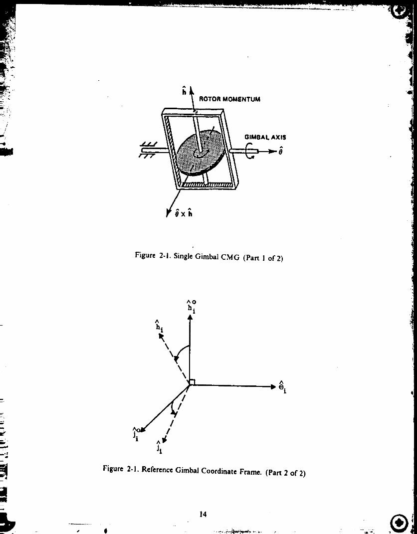
Figure 2-1. Single Gimbal CMG (Part i of 2)

AO

h i

A

h!

\\

J!

A

L Oiw

Figure 2-1. Reference Gimbal Coordinate Frame. (Part 2 of 2)

0

14 ®

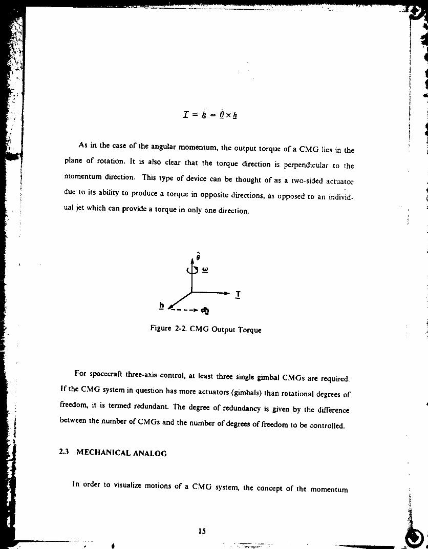
As in the case of the angular momentum, the output torque of a CMG lies in the

plane of rotation. It is also clear that the torque direction is perpendicular to the

momentum direction. This type of device can be thought of as a two-sided actuator

due to its ability to produce a torque in opposite directions, as opposed to an individ-

ual jet which can provide a torque in only one direction.

Figure 2-2. CMG Output Torque

For spacecraft three-ads control, at least three single gimbal CMGs are required.

if the CMG system in question has more actuators (gimbals) than rotational degrees of

freedom, it is termed redundant. The degree of redundancy is given by the difference

between the number of CMGs and the number of degrees of freedom to be controlled.

2.3 MECHANICAL ANALOG

in order to visualize motions of a CMG system, the concept of the momentum

15

nllll

linkage [1] is introduced and the analogy to a robotic manipulator is proposed. Con-

sider the CMG system as an open-loop kinematic chain or linkage made up of equal

"length" momentum links, placed in arbitrary order, with one link attached to a

grounded pivot. The "length" of each link is given by the magnitude of each CMG

angular momentum, considered equal in this case. The individual links are constrained

to rotate in a fixed plane determined by the corresponding gimbal axes. The moti-

vation for this concept derives from the expression for the total angular momentum of

a CMG system as the vector sum of individual momenta. The summation operation in

this case is commutative. For a robotic manipulator, the end-effector position is the

vector sum of the individual link displacements, it is proposed that a correspondence

exists between link displacements for a manipulator and individual momenta for a

CMG system. The first part of the analog then, is the correspondence between angular

momentum for a CMG system and displacement for a manipulator.

',a

t

The momentum linkage can be defined as a commutative linkage with links made

up of individual momenta, /1, [l]. The total system momentum corresponds to the

position of the momentum linkage tip in momentum space which is a Euclidean

3-space /:9. We can think of the momentum linkage as a manipulator whose end-effec-

tot oosition corresponds to total angular momentum. The workspace of this manipula-

tor naturally corresponds to the momentum volume and the boundary of the

workspace is defined as the momentum envelope or locus of all points traced out by

the maximally stretched momentum linkage. An example of the momentum envelope

[br 4-P.vramid mounted CMGs is shown in Figure 2-3, [i]. The holes or funnels rep-

resent windows on the envelope. These regions represent unattainable momentum

16

MOMENTUM ENVELOPE FOR 4-PYRAMID MOUNTED SG CMGs(_ = ,54.73o)

ZA

e3 02

Y

CONSTANT MOMENTUM

LINES

A

e4X

4--PYRAMID MOUNTED SG CMG=(SKEW ANGLE'S' - ,54.73"}

Figure 2-3.Momentum Envelope For 4-Pyramid Mounted CMGs

17

states, because the normal to the window is aligned with a gimbal axis. The funnel then

is part of the boundary to the momentum volume.

The momentum linkage concept was used in [1] to describe the total angular

momentum of a CMG system and to describe the boundary surface or momentum

envelope as the surface generated by the stretched momentum linkage. The linkage

concept was also used to describe null motion of a CMG system, which are discussed

in the next section.

2.4 TORQUE AND NON-TORQUE PRODUCING MOTIONS

The output torque for a system of n CMGs is given by the time rate of change of

the total system angular momentum relative to a frame of reference of interest, in this

case the spacecraft body-fixed coordinate frame, which is given by:

! = _h(O)= g(o) (2-3)

where J(o) = [ b(o,) ..... _.(o,,) ], t.._ta.t.._o.._ J,_ob,.,, ,_,_tr_.,:(3 × .)

Oh Oh_,ji(Oi) = "- = _, Jacobian columns

It is seen that the total output torque for a system of CMGs is given by the sum of

the individual gimbal torques. Extending the momentum linkage concept to this case,

the motion (rotation) of each link corresponds to the output torque for each C.MG.

I'o draw the analogy' to the robotic manipulator, it is noted that for the manipulator

the end-effector velocity is the vector sum of the individual link velocities. Just as the

!

18

®

individual link displacements correspond to angular momenta, link velocities corre-

spond to individual CMG output torques, thus the total output torque for a system of

CMGs corresponds to the velocity of the momentum linkage tip in E_. So far it has

been established that for the mechanical analog to a CMG system (the robotic manip-

ulator), link l_'egths correspond to magnitude of individual CMG angular momenta,

and end-effector position and velocity to total angular momentum and total output

torque for the CMG system. What remains to complete the analogy is to show an

equivalence in the singularity problem for a manipulator and the ('.MG system.

We now turn our attention to torque and non-torque producing link motions (or

gimbal rates). First, the linkage concept will be used to describe torque and non-torque

producing motions, and then an analytic description in terms of gimbal rates will be

presented.

Using the momentum linkage concept, it is seen that the total output torque of a

CMG system corresponds to the velocity of the linkage tip. If the linkage tip is station-

ary, no net torque is applied to the spacecraft. Torque producing motions are those

link motions for which the tip of the momentum linkage moves. On the other hand,

relative motions of the links that do nor affect the location of the linkage tip do not

produce a net torque on the spacecraft, and are termed non-torque producing rnotions.

These motions can be visualized by treating the linkage tip as a virtual pivot, which

fixes the tip location, and moving the remaining links. The linkage can attain any

kinematically admissible configuration or "closure", by relative link motions as long as

the linkage tip remains stationaD'. These relative motions are termed "admissible". An

example of such a motion for the mechanical analog is shown in Figure 2-4. The cho-

19

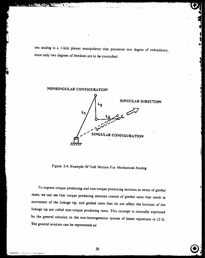
sen analog is a 3-1ink planar manipulator that possesses one degree of redundancy,

since only two degrees of freedom are to be controlled.

6

NONSINGULAR CONFIGURATION

_L 2 SINGULAR DIRECTION

/ .

"" SINGULAR CONFIGURATION

Figure 2-4. Example Of Null Motion For Mechanical Analog

To express torque producing and non-torque producing motions in terms of gimbal

rates, we can see that torque producing motions consist of gimbal rates that result in

movement of the linkage tip, and gimbai rates that do not affect the location of the

linkage tip are called non-torque producing rates. This concept is naturally expressed

by the general solution to the non.homogeneous system of linear equations in (2-3).

The general soiution can be represented as:

20 ®

where

O_= +Particular solution (J(O) OI, = T )

Homogeneous solution (J(O_) O_H = O_)

The particular solution expresses the torque producing gimbal rates, and the homoge-

neous solution the non-torque producing gimbal rates or "null motion". The term "null

motion" arises from the fact that the solution to the homogeneous system consists of

gimbal rates that lie in the null-space of the Jacobian matrix, and therefore produce no

instantaneous torque ("instantaneous" because the Jacobian matrix is evaluated using

the instantaneous values of the gimbal angles). These "null motions" are the variations

of "adrrfassible" relative link motions. This property of null motion can be exploited to

reconfigure the linkage or momentum _tate of the CMG system without altering its

total momentum. Correspondingly, torque producing gimbal rates lie in the row space

or orthogonal complement of the null-space of the Jacobian. The solution-space to the

non-homogeneous problem can be regarded as 2-dimensional, with an orthogonal basis

consisting of the torque and non-torque producing solutions•

The system of linear equations (2-3) can be solved as long as the rank of the Jaco-

bian matrix is 3. If the rank is less than 3, the CMG system cannot produce a torque

along all three axes of the spacecraft, and three-axis controllability is lost. The CMG

system is termed singular when the rank of the Jacobian is less than 3, i.e. the matrix is

singular. This essentially defines the singularity problem for CMGs. In this situa:ion

no output torque is available along an axis or direction. This information will now be

used to establish the equivalence of the singularity problem of a CMG system to that

of a corresponding manipulator.

21

,

+Jq

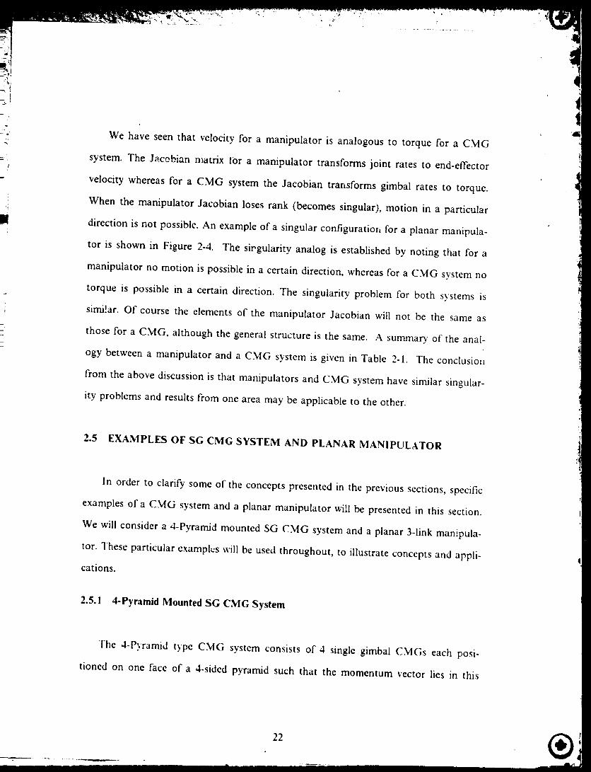
We have seen that velocity for a manipulator is analogous to torque for a CMG

system. The Jaccbian matrix lor a manipulator transforms joint rates to end-effector

velocity whereas for a CMG system the Jacobian transforms gimbal rates to torque.

When the manipulator Jacobian loses rank (becomes singular), motion in a particular

direction is not possible. An example of a singular configuratio** for a planar manipula-

tor is shown in Figure 2-4. The sirgularity analog is established by noting that for a

manipulator no motion is possible in a certain direction, whereas for a CMG system no

torque is possible in a certain direction. The singularity problem for both systems is

simi!ar. Of course the elements of the manipulator Jacobian will not be the same as

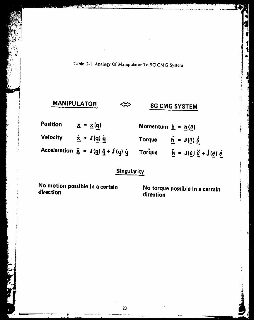
those for a CMG, although the general structure is the same. A summary of the anal-

ogy between a manipulator and a CMG system is given in Table 2-1. The conclusion

from the above discussion is that manipulators and CMG system have similar singular-

ity problems and results from one area may be applicable to the other.

2.5 EXAMPLES OF SG CMG SYSTEM AND PLANAR MANIPULATOR

In order to clarify some of the concepts presented in the previous sections, specific

examples of a CMG system and a planar manipulator will be presented in this section.

We will consider a 4-Pyramid mounted SG CMG system and a planar 3-1ink manipula-

tor. These particular examples will be used throughout, to illustrate concepts and appli-

cations.

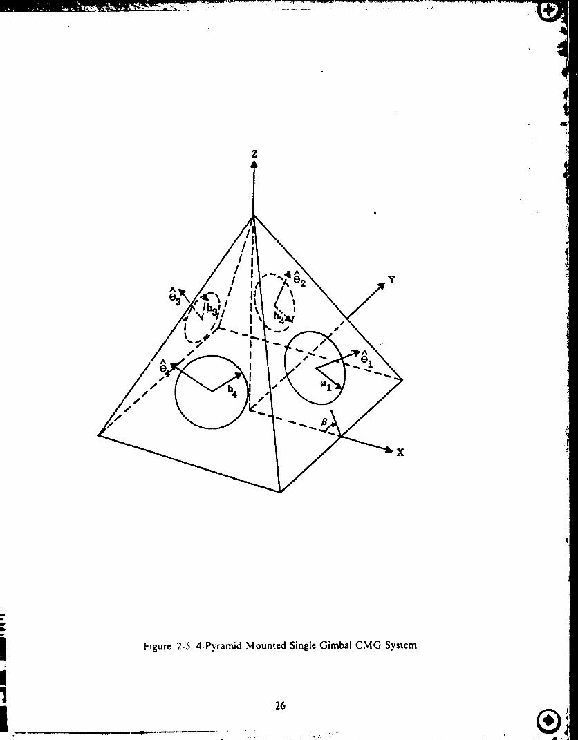
2.5.1 4-Pyramid Mounted SG CMG System

['he 4-Pyramid type CMG system consists of 4 single gimbal CMGs each posi-

tioned on one face of a -l-sided pyramid such that the momentum vector lies in this

22 ®

/; !

Table 2-1. Analogy Of Manipulator To SG CMG System

MANIPULATOR <¢¢> SG CMG SYSTEM

Position x = x(q) Momentum h = h(O)

Velocity x_ = J (q_)q_. Torque h_"= J (__)t

Acceleration _ - J(_) _, J(g) _ Tor¢lue i_ = J(#) _ * j(e) t

Singularity

No motion possible in a certaindirection

No torque possible in a certaindirection

t

)

t

23

plane. An example of this mounting configuration in the spacecraft body fixed coordi-

nate frame { X,Y,Z} is shown in Figure 2-5. lfthe skew angle//equals 54.73 degrees,

the gimbal axes lie along the main diagonals of a cube.

We will express the angular momentum of each CMG with respect to the space-

craft coordinate system. These are given by:

ic snol[h_ = h cos01 _2 = h

s/3 sin 0 l

h3 = h -cos03 h_ = h

s// sin 03

COS 0 2

- c_ sin 0.

s/3 sin 02

cos 04 1c/_ sin 04

s]3 sin 04

1i

,!

1

where #3 = sin/_

= cos//h = ,4,_gular momentum magnitude

The total angular momentum of this system is:

_h =_h, + __h2 + h 3 + h (2-4)

The output torque of the CMG system is obtained by differentiating (2-4) ira the space-

craft frame of reference:

The Jacobian matrix has the form:

24

- cfl cos O, sin 02 cfl cos 03 - sin 04h - sin 01 - c/_ cos O: sin 03 cfl cos 04

s/] cos 0_ s/3 cos 02 s/_ cos 03 s/3 cos 04

(2-6)

A method for constructing the null-vector(s) of the Jacobian matrix using the concept

of the generalized cross-product in n-dimensions is presented in the next section. It

will be shown that much insight about the properties of the null-space can be gained

through this construction method.

2.5.2 Null-Space Of Jacohian Matrix And The Generalized Cross-Product

It has been shown that the null-space of the Jacobian contributes the homogene-

ous or non-torque producing solution to (2-3). The null-space basis vectors are essen-

tial, because the homogeneous solution ca '. be written as a linear combination of these

vectors, as well as providing more insight into the kinematics of the CMG sx'sT: :n. The

dimension of the null-space or nullity [2] is:

n(J) = n - r(J) 12-0t

where n(J) = Nullity cf Jacobian

r(J) = Rank of Jacobian

n = Dimension of Jacobian domain space

For this CMG configuration, n = 4. When the Jacobian is non-singular, its nulhty is

1, and when it is singular its nullity is 2 (due to non-coplanar gimbal mounting). The

null-space basis vectors can be determined by row-echelon reduction of the Jacobian to

produce its dependent columns, which then can be used to span the null-space. This is

25

g

A

II

Figure 2-5.4-Pyramid Mounted Single Gimbal CMG System

26

a numerical method and does not provide a closed form expression for the basis vec-

tors. A closed form expression can be generated by use of the generalized vector cross-

product in n-dimensions [1] . This method generates an orthogonal basis by forming

n- rank(J) vectors that are orthogonal to the linearly independent r_w vectors of the

Jacobian and to each other. This approach is pret_rred over the row-echelon method:

not only because a closed form solution is obtained, but also for the general insight

that it provides about null motion.

t41

To n'otivate this approach, it is noted that the rank of a matrix is given by either

the column rank or the row rank, since the column rank equals the row rank [2]. Let

_; denote an n-dimensional null-vector of J(_0) . This vector must satisfy J(__0)v = 0.

For the case when Jlt)) is nonsmgular, it has three linearly independent row and col-

umn vectors, and rank(J) -- 3. Therefore. the nullity is I, and '£ must be orthogonal

to the row vectors of J(0). lo cart', out the cross-product in n-dimensions, it is noted

that the cross product of two vectors in 3-dimensions can be written in terms ol their

components as a 3x 3 determinant. These components are the 2x 2 minors of this

3 x 3 matrix. Let u,,, illustrate this b'_ an example. Consider two 3-dimensional vectors

_,A._hexpressed in a rectangular coordinate system with unit vectors i ,j, k . Then

we can write:

A A A

_A= a_i + ayj + a.k

A A A

t2 = h_i + hvj + h:k

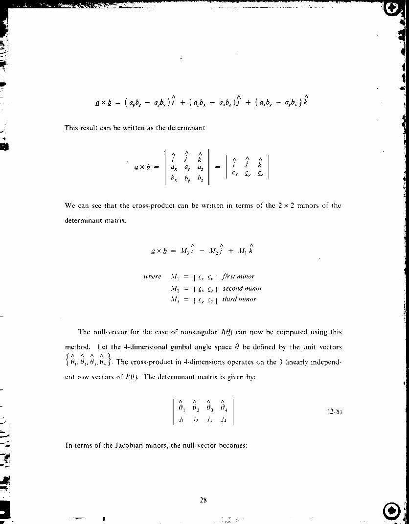
lhe cross-product of_d and h ts given by:

L 27

P 4

a ×b = ( .,¢ - ^ ^

This result can be written as the determinant

axb =

A A, Ai J k

a x ay a z

bx by be

A 5 Ai J k

cx _cy cz

We can see that the cross-product can be written in terms of the 2 x 2 minors of the

determinant matrix:

A A A

a× b -- -_'13i -- -_12j + .ll I k

where 311 = I C__c_v] first minor

M2 = I _c, _cz I second minor

._[3 = I cy c.z I third minor

The null-vector for the case of nonsingular J(0) can now be computed using this

method. Let the 4-dimensional gimbal angle space _0 be defined by the unit vectors

A A A A }0t, 0,, 03, 0_ . The cross-product in 4-dimensions operates c,a the 3 linearly independ-i

ent row vectors of J(0_). The determinant matrix is given by:

A A A &

01 0 2 O_ Oa

a., 5 #

In terms of the Jacobian minors, the null-vector becomes:

2_

(2-8)

A A A A

v = ._/40, - ._1302 + M203 - ,_I_04O¥

V

313

._t2

311

(2-9)

where = I.!, 4243 I. z2= I d, d2d_=I

This method can also be used when the Jacobian is singular. In that case, J(0_) will only

have two linearly independent row vectors, thus in order to apply this method, these

row vectors must first be determined. ]he next step would be to take the 3-dimensional

cross-product using only the first three elements of the row vectors in order to generate

a vector in 3-space that is orthogonal to the truncated row vectors. Then, a 4-dimen-

sional cross-product is taken using the two linearly independent row vectors and the

vector just generated with a zero fourth element. In this way, the two orthogonal null-

space basis vectors are generated. We can apply this approach in a similar fashion to

systems with more than 4 CMGs.

Considerable insight can be gleaned from the form of the null-vector and the Jaco-

bian minors, in general, this expression (2-9) for the nuii vector is valid when J(___)is

nonsingular, and it is a function of the gimbal angles. The nunors of the Jacobian

matrix have a very interesting physical meaning. A minor is zero when the columns of

the minor matrix or 3 × 3 Jacobian sub-matrix are dependent. This means the sub-ma-

29

trix is singular, and its columnsdo not span U. The rank of this submatrix has

dropped from 3 to 2. Physically, it means that the 3 CMGs corresponding to this sub-

matrix can no longer produce torque along all three spacecraft axes, hence three-axis

controllability is lost for this CMG sub-system. We can thus think of the minors as

controllability tests for sub-systems of 3 CMGs taken together according to the col-

umns in the corresponding minor. For example, sub-system ! corresponding to 3I_

would be comprised of CMGs 1, 2, and 3. It is clear that when all 4 sub-systems lose

three-axis controllability, the spacecraft is not controllable bv the CMG system. An

alternate statment is that the rank of a matrix is the order of the largest nonsingular

square sub-matrix formed from this matrix [-2]. Thus the Jacobian is singular when all

3 x 3 minors are 0, i.e. there is no nonsingular sub-matrix of order 3. It is also evident

that when one of the minors is zero. one of the elements of the null-vector is zero.

which implies that no null motion is available from the corresponding CMG.

2.5.3 Planar 3-Link Manipulator

A planar 3-1ink manipulator with i degree of redundancy is shown in Figure 2-6.

The choice for generalized coordinates in this case are the absolute joint angles. This

choice of coordinates is made to keep the analogy to the CMG system transparent.

The link length choice is dictated by the requirement that the manipulator possess the

same number of equivalent types of singularities. We could have chosen equal length

links tbr the manipulator to match the choice of equal magnitude angular momenta.

but this would have resulted in a manipulator that would not possess all types of sin-

gularities encountered in the CMG system. Specifically. internal Elliptic type smgulari-

30

g -..y,....,,

®

ties would not be encountered for this manipulator (the various types of singularities

will be defined in Chapter 4).

Y

Lq

L L3

Figure 2-6. Planar 3-Link Manipulator

The motion of the manipulator is described by the generalized coordinates

{ qt, q2, q_ } relative to a fLxed coordinate frame { X, Y }. The displacement of the end-

effector is denoted x, while the individual link displacements are defined by x.. The

link displacements are:

[ ] [co,q3]cosql _x2 --- ! x 3 = I&l = 21 sinqt sinqa sinq3

31

.... _ *_mul_._ _¢dl _

where l = Link length

The end-effector position is given by:

_x = _rI + __x2 + _x3 (2-]o)

The end-effector velocity thus becomes:

= _ + x-2 + _3 = J(q) q

The Jacobian matrix for the manipulator is:

r- --2sinql --sinq2 --sinq3 ]J(_q) = l [ 2 cos ql cos q2 cos q3

(2-11)

(2-12)

Comparing the manipulator results to the 4-CMG system, we can easily see an analo-

gy. Observe that the manipulator Jacobian has a similar form to the CMG Jacobian

with this choice of generalized coordinates. Specifically, the manipulator colurrms are

the partial derivatives with respect to the generalized coordinates of the individual joint

displacements, as was analogously true for the CMG system, it is also noted that if

the Jacobian is differentiated again, with respect to the generalized coordinates, its col-

umns will be the negative of the link displacements. This is due to the cyclic nature of

the trigonometric functions, governing the generalized coordinates, hence is also true

for the CMG Jacobian. Finally, it is emphasized that the planar manipulator of

Figure 2-6 is not the exact analog to the 4-CMG system because its Flliptic type intcr-

nal singularity is actually a degenerate l lyperbolic singularity. This will become clear m

Chapter 4. The exact analog can be obtained by projecting the gimbal motions in the

32

3 orthogonal planes formed by the spacecraft coordinate system. A manipulator with

varying link lengths can then be defined such that its motion recovers the motion of

the gimbals in each plane. A simple example would be to project the motion of gimbal

#1 in the X - Y plane. The path of the gimbal in this plane is elliptic because the pro-

jection varies. A link with varying length can be used to duplicate this motion in the

plane.

The null-vector for the manipulator Jacobian can also be constructed using the

generalized cross-product approach. Let the 3-dimensional joint angle space be defined

{A A A }by the unit-vectors qL, q:, q_ • The cross-product in 3-dimensions operates on the 2

linearly independent rows of J(_q). The determinant matrix is:

A A A

q_ q2 q3

J_', v5(2-13)

In terms of the manipulator Jacobian minors, the null-vector becomes:

A_v = .xlr3 _, - ._,12_2 + ._,/,q3

or

,I,l3

E = -- ,_'/2

3,11

(2-14)

.u, = I

Equivalent comments apply to the manipulator null-vector as for the CMG null- 6

vector. The physical meaning of the minors in this case represents relative folding of

the links. When a minor has 0 value, the columns of the corresponding sub-matrix of

order 2 are not linearly independent; the sub-matrix has rank 1. This implies that the

velocity capability of these two links is restricted to a line rather than a plane whenever

the minor is nonzero, therefore the links are colinear or folded. The value of each

minor thus represents the degree of folding of the corresponding pair of links. In this

case there are 3 distinct combinations of pairs of links; when all three combinations are

singular, the Jacobian is also singular, thus motion is restricted to a line. The general

concepts of controllability, capability for null motion, etc. naturally carry over from the

previous discussion about the CMG Jacobian null-space and will not be repeated here.

J

v

34

Spacecraftattitude controlmay be realizedthrough angularmomentumexchange

betweenthe spacecraftand momentumstoragedevicessuchas singlegimbalCMGs,

whichcanbe usedto providecontrol torquesfor attitudecontrol of spacevehicles.A

most commonexampleis the reorientationof a spacecraft. The most generalpre-

scriptionfor anattitudemaneuveris to specify the desired final state (attitude and rate)

given the initial state of the spacecraft.

request using C*IGs as ectuators.

"[he controller must then be able to satisfy this

An attitude maneuver can be accomplished in various ways. The methods to

accomplish these maneuvers can be classified as kinematic or dynamic, depending on

the criteria used. An example of a kinematic approach is an eigenaxis or single-axis

rotation, because this results in the smallest rotation angle required tbr the maneuver.

A single-axis feedback controller based on this approach is used on the Space Shuttle

[3]. On the other hand, the OI,GX controller [4] is an example of a dynamic approach.

It uses a feedforward-fccdback model-following controller structure for fuel-optimal

maneuvers, which are not constrained to rotations about a single axis. This approach

reduces fuel consumption, hence it is superior to the kinematic method. For the case

of spacecraft with CMGs, a model tbllowing controller (dynarmc method) could also be

used, as long as the model or dcsircd traiector3 is constructed in a _av that rcllects the

unique properties of (;MG actuated spacecraft.

.................. ;.............0

35•14

Onemethod of generatinga desiredtrajectory that is globally "optimal" in a cer-

tain sense,usingthe calculusof variations,is describedin [5]. The optimization prob-

lem requires the design of an optimal terminal controller, with only some of the states

specified at a fixed terminal time. These specified states are chosen to be the spacecraft

initial and teminal attitude and rate. The assumption of no external torques implies

that the terminal CMG state is not constrained, since that would violate conservation

of angular momentum for the combined system.

Performance criteria of interest include minimization of gimbal rates, minimization

of final spacecraft state error from the desired value, and maintaining CMG 3-axis

controllability over zhe entire trajectory. Redundancy resolution can be accomplished

in a global sense by parametrizing CMG 3-axis controllability Over the whole space-

craft trajectory. Solution of this problem, however, is very. difficult because some of the

Lagrange multipliers have no boundary conditions at either end (i.e. initial and termi-

nal conditions), since we have specified the values of the corresponding states at both

ends. An intial control history is required to solve this optimization problem.

To represent the attitude of a spacecraft, Euler parameters { r/, _ } or quaternions

will be used. Let the underscore represent a vector expressed in the spacecraft fixed

frame. The rate of change of the l-uler parameters is given by [6]:

IYLet _qrepresent the quaternion,

_-- _ i__/_T(. O2 -- --

1 x

36

(3-1)

It,

then we can rewrite (3-1) as:

= E(q)co (3-2)

The equations of motion for the combined spacecraft-CMG system are obtained from

the total angular momentum expression. Let the superscript I denote a quantity

expressed in an inertial frame. ]he total angular momentum expressed in an inertial

frame is given by:

I_[_ = l_[ 1 + hi f3"31

o

where [___tI = Spacecraft angular momentum ( It' = I c,)' )

h I = Total C3IG angular momentum

Expressing the time rate of change of the absolute total angular momentum of the

combined system in the spacecraft fixed body axes, we obtain:

t1 + e) xll + h + o) xh = l_" (3-4)

where 1_"= External torques on spacecraft

Rewriting (3-4) with/4 = J0_ , and including (3-2) we obtain the dynamical equations

governing this system:

37

_q = E(__q)co

m = - I-' [ co× ( to+,+ +(_o)) ] - t-' JCO_)o_+ t-' _r(3-5)

3.2 CONTROL ARCHITECTURE

Attitude maneuvers of spacecraft equipped with CMGs are usually accomplished

using a dual-level control architecture. This is because we can consider the attitude

maneuver as consisting of two parts; first, the necessa_' torque required from the

CMG actuators to accomplish the maneuver must be determined, and second, this tor-

que must be gcnerated by the redundant system of CMGs. These two levels of the

controller are defincd as:

a) Outer Control l+oop

b) Inner Control Loop

The general objectives of the control system for the combined spacecraft-(2MG system

can be stated as:

a) Spacecraft reorientation accomplished using SG CMGs.

b) CMG system must supply a commanded torque while avoiding singular config-

urations.

c) Spacecraft controllability must be maintained at all times.

38

It hasbeenshownthat singlegimbalCMG systemsareplaguedby singularstates.

For this reason,the Inner Control Loop must be capableof generatingthe required

torquewhile simultaneouslyavoidingsingularconfigurations.This is not aneasytask.

This problem might be made more tractable if the Outer Control Loop design takes

this adverse feature of single gimbal CMGs into account; specifically, the design of the

Outer controller must tolerate occasional errors in torque delivered by the CMG sys-

tem, or limit the CMG torque command to avoid approaching vicinities of singular

CMG oriehtations. The capability of accomodating errors in the torque request, is

required due to reduced effectiveness of the CMG system near singular configurations.

The Outer controller should also not constrain the CMG s_,stem to produce a given

torque if this can lead to a sin t_ularity which the Steering law is not capable of avoid-

ing. !n addition, the non-spherical nature of the SG CMG momentum envelope must

specifically be taken into account for maneuvers which move the CMG system near

saturation.

All currently propesed SG CMG Steering laws (including those presented in this

thesis) are unable to guarantee continuously flawless singularity avoidance, although

various techniques (discussed in Chapters 5 and 6) do aid in reducing singular encount-

ers. Because of this, any Outer controller must be prepared to occasionally deal with

singularity related phenomena as discussed above. For reorientation maneuvers, the

vehicle trajectory may be as general as possible, since the only constraints are the two

boundary conditions; the initial and final states of the spacecraft. The choice of inter-

mediate points is arbitrary, and thus may be chosen, if required, to aid in avoiding sin-

gular CMG configurations.

3.3 OUTER CONTROL LOOP

The function of the Outer Control Loop is to generate torque commands that

accomplish the spacecraft attitude maneuver. Two pcssibilites for this controller were

mentioned in the previous section. The model following controller can be implemented

in different ways; two examples are the Sliding Mode Controller (SMC) and optimal

tracking method. An example of the Sliding Mode approach applied to spacecraft

using CMGs can be found in [7], where the control input __ is defined as the output

torque of the CMG system:

"r_= J(O_)O_

The advantages of this approach are real-time implementation and a globally stable

controller based on Lyapunov stability analysis, despite the presence of model impre-

cision and disturbance torques.

A tlerivation of the optimal tracking method for spacecraft using CMGs can be

found in [5]. The solution to the tracking problem leads to a full-state feedback c.7,ntrol

law where the optimal control has a feedforward-feedback structure. The major advan-

tage of this approach is that performance criteria of interest can be included m the

objective function. This approach is not considered real-time implementable however,

since it requires numerical solution (an initial ,.ontrol history, is required to start the

numerical process _.

4O ®

• _r, _::',,_.,'r_*_-y'.,_._ _,'_ _ _..- -- - • _ , .

3.4 INNER CONTROL LOOP

The function of the Inner Control Loop is to generate gimbal angle rate com-

mands that cause the CMG system to produce the desired torque requested by the

Outer Control Loop. It must also resolve the redundancy present in the CMG system.I

In the literature, this is usually referred to as a Steering law. This is not the only

approach available. The Steering law may also be formulated to generate gimbal angle

cormnands in response to angular momentum requests [8]. [he Steering law thus

exploits the kinematic relationship between CMG gimbal rates and the rate of change

of total CMG angular momentum in the rotating frame of reference (spacecraft body

fixed frame).

The requirements that a successful Steering law must meet are:

a) Generate the required torque.

b) Steer the gimbal angle trajectories away from undesirable configurations.

c) Meet any constraints placed on the CMG system, such as maximum gimbal

rates, gimbai stops etc.

An undesirable configuration is one for which the ('MG system is unable to produce

any torque along a particular dm.ction in _ . This is equivalent to loss of spacecraft

three-axis controllability, thus conditions al and b) are not independent in the sense

that the ability to produce a required torque implies that the CMG system is not in an

undesirable contiguration.

41

/

To produce a desired torque reqmres the solution of the underdetermined system of

sinultaneous linear equations given by:

The general solution to a non-homogeneous system of linear equations such as (3-6),

can be formed from the solution to the homogeneous system, and an}' particular sol-

ution, as was discussed in Chapter 2. When the rank of the ]acobian matrix is 3, infi-

nitely many solutions to (3-6) exist. In this case, the particular solution is almost

always obtained using the Mome-Penrose pseudoinverse [2] , which is given by:

|

Op = ]r(jjT)--Iv_- ',3-7)

To illustrate the properties of (3-7), a derivation based on orthogonal projections ts

presented in the next sectioo, To motivate this derivation the properties of the the

Moore-Penrose pseudoin;erse are presentcd below:

a) 0e is orthogonal to _.. The, efore, < 0_e,__:, > = O.

b) The particular solution is the minimum norm solution to (3-67, as can be seen

from the Pythagorean theorem:

I_012 10_ 1 I= +10_,,

Since the particular and homogeneous solutions are orthogonal to each other.

the norm of the solution will be smallest when the homogeneous solution is

zero.

p,

42

,i

/

3.4.t Derivation Of The Moore-Penrose Pseudoinverse Using Orthogonal Projections

From the fundamental theorem of linear algebra [9], the row space of an,,' matrix

is perpendicular to its nullspace. Since the torque producing solution lies in the row

space of J, we can write the general solution to (3-6) in the form:

where

0_=0_. o,O_R = Torque producing solution [ J O R = _ )

0__,,= Ilo,nogeneous solution ( J O_v = _) )

The torque producing solution can now be written as a linear combination of the row-

space basis vectors. Since the Jacobian matrix is nonsingular, it has 3 linearlx inde-

pendent row vectors. The row space is spanned bx these vectors (which become the

columns of jr}, thus we can write tile torque producing solution _s:

i,

?f

wf

where _R_T = i th Jacobian row vector

Substituting (3-8) in (3-6) we obtain

jjr_ = r

from which we can solve for _:

__ = ( jjl" )--I __

43

13-tI_

i

To obtain the final result for _OR we substitute (3-% into (3-8) to get:

O-e= ]r(JJr)-_z (13-1o)

'8

This is the desired final result. By picking the particular solution as (3-10), the proper-

ties of the Moore-Penros.e pseudoinverse are satisfied. Since the pseudoinverse provides

the minimum 2-norm solution, an alternative derivation can be obtained using

Lagrange multipliers to solve the following problem:

! 07-0nun T

subject to J -O = z_

I OTO+ JO)wtth tlamihonian !I = _ ....

This minimization will yield 0__= 0h, as defined in (3-10):

The homogeneous solution can be written as a linear combination of the Jacobian

null space basis vectors.

O_tt = ).,.It) v, 13-1 I)

n -- r(,D

V

where ).,(t) = lime varying scalar weighting fiTctor

v, = n - dimensional Jacobian mdl space basis vector

rlJ) = Rank oJ'Jacot, ian

The computation of the null space basis vectors is carried out using the generalized

cross-product approach as presented in (Thapter 2. The scalar weighting factor deter-

..... 7

..14

......... "7-.".• :_

mines the magnitude and sign of the contribution of each null space basis vector to the

homogeneous solution. These are the free design parameters, to be selected in a man-

ner that the performance criteria for the Steering law are accomplished.

Because "_0Ris orthogonal to _,v , any general solution to (3-6) can be written in

terms of the Moore-Penrose pseudoinverse and any homogeneous solution. An alter-

native approach for a Steering law utilizing linear prograrrmfing is discussed in the next

section.

3.5 REDUNDANCY RESOLUTION VIA LINEAR PROGRAMMING

Another way of addressing the singularity avoidance and s:eering problem is to

assign gimbal rates via linear programming, as described in [10]. The instantaneous

torque output of each gimbal is used to form a set of activity vectors that are used to

satis_' spacecraft rate-change requests by solving for approximate gimbal displace-

ments, or torque requests by solving for instantaneous gimbal rates. The linear pro-

gram intrinsically incorporates upper bounds on the CMG selection that limit allowed

gimbal displacements and rates while optimizing an objective function to encourage

avoidance of singular configurations and gimbal stops, t?nfortunately, this method like

all available methods, cannot avoid all internal singularities due to the use of a gra-

dient-based objective (to be discussed in Chapter 5). Linear programming has been

applied to double gimbal CMGs, however, with considerable success.

lhis approach can also account tbr hybrid control of spacecraft using both jets

and CMGs. It is highly adaptable to hardware failures, variations in CMG system deft-

45

- Illr

L

nition, and changes in vehicle mass properties. A major advantage of this approach is

that performance" criteria can be explicitly and dynamically taken into account merely

by altering the linear objective functions and imposed upper bounds.

46 ®

CHAPTER 4

SINGULAR CONTROL MOMENT GYRO (CMG) CONFIGURA-

TIONS

4.1 DEFINITION OF SINGULARITY

Spacecraft attitude control systems utilizing single gimbal CMGs must effectively'

address the singularity conditions inherent with this type of actuators. These conditions

prevail when the CMG system is in a configuration that precludes torque generation in

a certain direction, i.e. spacecraft three-axis controllability is lost. These conditions, if

not properly addressed, severely limit the usable momentum capability of the CMG

system. Not only must the singularities themselves be avoided; neighborhoods of sin-

gular states represent regions of limited torque capability, thus require high gimbal

rates to generate the requisite torque. I lardware limits on gimbal rates therefore entail

that these neighborhoods also be considered in the control law design.

The requirement of spacecraft three-axis controllability is expresscd by the rank of

the CMG system Jacobian matrix. If the rank of the Jacobian is less than 3, the CMG

system is unable to produce torque along a direction __u,referred to as the singular

direction in /:'_. This is summarized below:

L a

Singular State: A singular state can be delined as a set of gimbal angles for which the

CMG system is unable to produce torque along the singular direction __u.This occurs

whenever rank(J) < 3, the number of controlled axes.

For 3-axis control the maximal rank of the Jacobian is 3 and the minimal rank is 2,^

because the gimbal axes, 0, are not mounted coplanar. For example, if rank(J)= 2,

47

the resultantotput torque liesin a planewhich is spannedby the columnsof theJaco-

bian matrix. The singulardirectionu is then perpendicular to this plane. This condi-

tion can be stated as:

.[i(Oi)T • u = 0 (i = 1,2,...,n) (4-1)

The gimbal angles corresponding to a singular configuration can be computed

using (4-1) and the expression for the Jacobian columns with respcct to the reference

gimbal coordina-te frame (2-1). The i 'h column of the Jacobian matrix is:

[ ^ ^ ])_'i= h cos Oij i o _ sin 0 i h i o (4-2)

Combining (,4-1) with (4-2) we obtain

A A oji.u__ = cosOi(Ji Oou) _ sinOi( hi ._u) = 0 (4-3)

the solutions of which are the singular gimbal angles, These angles are obtained from:

0 s = tan-IA

_t hi o • u__

{4-4)

where O__. = Singular gimbal angle ( 2 solutions )

,i= +1

The two solutions obtained from (,.1-4) correspond to the two extreme projections of

the i'_ angular momentum vector on the singular direction. These are the maximum

positive and maximum negative projections, therefore there corresponds two solutions

0

,18

. . ; '- _,l_s _

for each singularity and momentum vector associated with maximum positive (+) and

maximum negative (-) projections along the singular direction. Examples of the vari- i

!] ous sign patterns can be found in [11] . The singularity problem can thus be summa-i

rized for a n-CMG system: There exist 2" combinations of gimbal angles for which the

CMG system cannot produce torque about any given direction in space [1].

All singular states can be classified according to their location in the total CMG

angular momentum envelope:

a)

b)

Surface or Saturation Singularities

Internal Singularities

i) Elliptic or Unescapable

ii) Hyperbolic

4.2 SATURATION SINGUL _,RITY

As the name suggests, a Saturation singularity corresponds to a configuration for

which the CMG system has projected its maximum momentum capability along a cer-

tain direction. A Saturation singularity can be defined as the set of gimbal angles for

which the total momentum of the CMG system lies on the momentum envelope

(implying that the momentum linkage tip has reached the momentum envelope). The

mechanical analog to this type of a singularity is a completely stretched manipulator.

Deeper insight about the Saturation singularity can be gained by examining the

behaviour of the momentum linkage. The momentum envelope, which is generated by

49

il

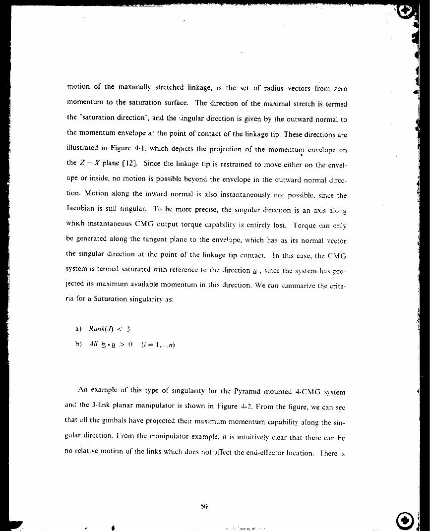
motion of the maximally stretched linkage, is the set of radius vectors from zero

momentum to the saturation surface. The direction of the maximal stretch is termed

the "saturation direction", and the ,,ingular direction is given by the outward normal to

the momentum envelope at the point of contact of the linkage tip. These directions are

illustrated in Figure 4-1, which depicts the projection of the momentum envelope onII

the Z - X plane [12]. Since the linkage tip is restrained to move either on the envel-

ope or inside, no motion is possible beyond the envelope in the outward normal direc-

tion. Motion along the inward normal is also instantaneously not possible, since the

Jacobian is still singular. To be more precise, the singular direction is an axis along

which instantaneous CMG output torque capability is entirely lost. Torque can only

be generated along the tangent plane to the enveJ_pe, which has as its normal vector

the singular direction at the point of the linkage tip contact. In this case, the CMG

system is termed saturated with reference to the direction _u, since the system has pro-

jected its maximum available momentum in this direction. We can summarize the crite-

ria for a Saturation singularity as:

t41dI

a) Rank(J) < 3

b) .4// h,._u > 0 (i= I ..... n)

An example of this type of singularity for the Pyramid mounted 4-CMG system

and the 3-1ink planar manipulator is shown in Figure 4-2. From the figure, we can see

that all the gimbals have prolected their maximum momentum capability along the sin-

gular direction. From the manipulator example, it is intuitively clear that there can be

no relative motion of the links which does not affect the end-effector location. There is

50

®

MOMENTUM ENVELOPE

Y

SATURATION DIRECTION

i

U

SINGULAR DIRECTION

h 1

MOMENTUM PROJECTIONS ON X-Z PLANE

X

Figure 4-1. Saturation Singularity Projections For 4-SG CMG System

no null motion possible for this type of singularity. A degenerate case where null

motion would be possible can be imagined if the ground pivot allowed rotation about

the singular direction, but this is excluded for this type of manipulator. The same com-

ments apply to the CMG system; For a maximally projected CMG linkage, no null

motion is possible (no degenerate case exists for the CMG system).

From the above discussion, it can be seen that a Saturation singularity corresponds

to the physical capabilities of the CMG system. Thus, the term "desaturation" refers to

the process by which the resultant momentum vector is removed or retracted from the

envelope or surface without net momentum transfer to the spacecraft. To accomplish

this task, an external torque (such as jet firings or gravity gradient/aerodynamic tor-

ques) is required to cancel the torque exerted cn the spacecraft while desaturating the

CMG system. Saturation states cannot bc avoided by the Steering law alone; A

51

momentum management procedure such as [13], [14] must be used to command the

spacecraft attitude such that the CMGs remain unsaturated.

CMG SYSTEM

Z

Y

cB cp' ] q • o

- C -9o'. ,8o',_)'.o" ]

[+. +, ._ +]

MECHANICAL ANALOG

Y

L 3

SINGULAR DIRECTION

o-c =:¢>

Q. 3,3'] Q>O

_ = Eo',o',o']

Figure 4-2. Example Of Saturation Singularity

4.3 INTERNAL SINGULARITIES

Any singular state for which the total angular momentum vector (or linkage) is not

completely stretched is defined by default to be an Internal singularity. These states

can be generated from the Saturation singularity by reversing one or more angular

momentum vectors so that they point opposite to the singular direction. [:or a

4-CMG system, these singularities can be gro_J.ped into two categories. One catego_'

consists of an even number of positive and negative projections, and the other category

is made up of an odd number of positive and negative projections. The mechanical

analog to this situation is a manipulator with folded links. Some singularities can offer

the possibility of escape through null motion, therefore it is useful to investigate the

conditions under which singular configurations can be removed by null motion alone,

and thus classify Internal singularities according to whether a null motion escape is

possible.

l

The term "escape" used in this context needs to be defined carefully. The term

escape will be defined in the following manner:

Escape By Null Motion: A singular CMG system can be reconfigured by null motion

into a non-singular configuration, if"one exists for the same total angular n_omentum.

The implications of this statement are twofold.

a) A non-singular configuration is reachable by null motion from t_ae singular-co-

nfiguration; i.e. the CMG system can be reconfigured in a continuous manner

777'U'II,.7.J.'......,

!:,i t

.a using null motion only. To state it succinctly, the two solution sets are not dis-

joint with respect to null motion.

[,t

i

b) The rank of the Jacobian can be affected (increased) by these null motion. The

singularity measure (to be introduced later) is increased also (can be made non-

zero).

An immediate consequence of these statements is that Saturation singularities are not

escapable. This will be established rigorously in the next section, when a test for the

possibility of null motion near a singularity is presented. It should also be emphasized

that the mere possibility of null motion at a singularity does not automatically' imply,

that the singularity is escapable. An example of this was given in the degenerate Satu-

ration singularity discussion for the manipulator.

al

ld

4.3.1 Test For Possibility Of Null Motion Near A Singularity

Valuable insi3ht can be gained by investigating the conditions under which null

motion is possible near a singularity. A method to examinine the behaviour ofa CMG

system using null motion near a singular state can be found in [1]. A similar approach

based on this method will now be presented. Let hS(Os) denote a singular CMG config-

uration. Expanding the total CMG angular momentum about about this singular con-

figuration, '_0s , we obtain:

- ore*)= ,=, 6P + 21 02h-i(_O_los 00_ + ll.O.T. ] (4-5)

54

i, |

The first partial on the right hand side of(4-5) is just the i '_ column vector of the Jaco-

bian. The expression for the second partial is given by:

i8

_ . A AJi = _'J_ Oi = O, Oi x ji = -- Oihi hi- _0_

02h, A----'--"=-- = -- h i h i : -- h_

If we now take the inner product of (4-5) with the singular direction, zd, the first term

on the right hand side drops out because the singu!ar direction is orthogonal to the

Jacobian columns, i.e. d_,(0_)• u = 0 . The resulting expression is:

Recognizing that the right hand side of(4-6) is a quadratic form. it can be written as:

- lborpb 0= 2 - - (4-7t

where P : diag{hi s. u) i = 1,2 ..... n

The diagonal matrix P will be refered to as the projection matrix, since its elements

represent the projections of the singular angular momentum vectors onto the singular

direction.

The governing equation for the null motion test is expressed by t4-7}, in order to

examine the behaviour of(4-7) for null motion near a singularity, the variatioqs in gim-

55

bal angles3/9,are defined to be null motion. For null motion, h = hs by definition,

since null motion do not affect the total angular momentum of the system. Therefore,

(4-7) becomes (neglecting the constant):

,50r p 60_ = o (a-s)

The null motion can be expressed as a linear combination of the null-space basis vec-

tors as in [15]. The gimbal angle variations can then be expressed in this basis as:

n-- r(.f)

0__0= _ ,a.__Vi= .\'X (4-9)i_--.|

where 2, = Scalar weighting factor

vi = Null space basis vector ( n -- dimensional )

r(j) = Rank of Jacobian matrix

Substituting (4-9) in (4-81, we obtain the desired final result:

_r Q_ = 0(4-10t

where Q = .v r p ,V

This quadratic tbrm can now be used to test the posslbtlit.v of null motion near a

singularity. Two possibilities exist:

a) Definite Q

56

b) Indefinite or Semi-Definite Q

4.3.1.1 Definite Q

If Q is definite, the quadratic form is defimte, and in order to satisfy (4-10) we

must have _ = O. This implies that no null motion is possible at this singular config-

uration, therefore no escape is possible from this singularity by null motion. Near a

singularity of this type, the CMG system cannot be reconfigured by null motion into a

non-singular configuration; the two configurations are disjoint solutions to the total

system momentum. This result can be used to idcnti_' unescapable singularities.

When P is definite, Q is also definite. This corresponds to the case of a Saturation

singularity, for which all angular momenta have maximum positive projections on the

singular direction. All the elements of the diagonal projection matrix are positive.

[his type of singularity was defined in [1] as Elliptic, because the quadratic in (4-7) has

the form of an elliptic conic section, an ellipsoid. Using this notation lbr the case of

definite Q, the singularity will be defined as Elliptic or unescapable. For Q to be defi-

nite, it is not neccessary that all momenta have positive projections on the singular

directions; i.e. P can be indefinite. Odd numbers of positive and negative projections

usually result in a definite quadratic form. A case for an even number of projections

has not been found for which the quadratic lbrm is definite.

4.3.1.2 Indefinite Or Semi-Definite Q

i •

The other possibility for (4-10) is to be either indefinite or serm-definite. It is

indefinite when the eigenvalues of Q are both positive and negative, and is positive

(negative) scmidctinite if Q has non-negative (non-positive) eigenvalues, i.e. has at least

57

!/

one zero eigenvalue [2] . in this case, _ = 0 satisfies (4-10). This implies that null

motion is possible at this singularity, therefore null motion may provide a possibility of

escape. In order to definitely state that escape is possible, degenerate solutions must

be excluded. Degenerate solutions are those for which rigid body rotation is possible

which does not affect the total system momentum. The term rigid body is used to indi-

cate the fact that the the singular configuration remains undisturbed during these null

motion. An example of this was given in "4.2 Saturatinn Singularity" for a manipula-

tor. In that case, the rigid body is the stretched linkage which can rotate about the

stretch axis. Similarly, it may be possible that the momentum linkage could possess

configurations for which rigid body rotations are possible.

|

41

]his type of singularity was defined in [I] as tlyperbolic because the quadratic in

(4-7) has the form of a hyperbolic conic section, a hyperboloid. Using this notation, a

singularity for which Q is either semi-definite or indefinite will be defined as t lyperbot-

ic.

Applying the above conclusions, the results of the null motion test can be used to

classiC" the two possibilities which exist for an Internal singularity:

a) Elliptic or I.lnescapable Singularity ( Q Definite )

b) Hyperbolic Singularity ( Q Indefinite or Semi-Definite )

It is evident that tlyperbolic singularities offer the posmbility of escape tt_rough null

motion. These cases must be examined ['or degenerate solutions to determine the possi-

bility of escape, l'_xamples of the various singularities are presented in the next section.

58 ®

4.4 EXAMPLES OF INTERNAL SINGULARITIES

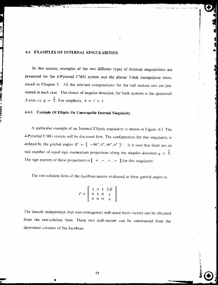
In this section, examples of the two different types of Internal singularitites are

presented for the 4-Pyramid CMG system and the planar 3-1ink manipulator intro-

duced in Chapter 2. All the relevant computations for the null motion test are pre-

sented in each case. The choice of singular direction, for both systems is the spacecraftA

X-axis, i.e. __u= X. For simplicity, h = l = 1 .

4.4.1 Example Of Elliptic Or Unescapable Internal Singularity"

A particular example of an Internal Elliptic singularity' is shown in Figure 4-3. The

4-Pyramid CMG system will be discussed first. The configuration for this singularity is

definedbv the gimbalangles:0_ = [ -90 °.0 °,90 °,0 °jr, It is seen that there are an

Aodd number of equal sign momentum projections along the singular direction _u = X.

The sign pattern of these projections is [- +, -, +. + ] for this singularity.

The row-echelon form of the Jacobian matrix evaluated at these gimbal angles is:

J

I I o 1 2eft0 I 0 I

o () 0 o

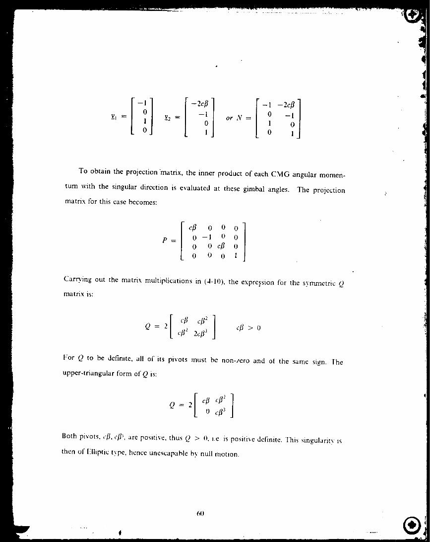
The linearly independent (but non-orthogonal) null-space basis vectors can be obtained

from the row-echelon form. These two null-vectors can be constructed from the

dependent columns of the .lacobian:

59

(

--10 v-21

0-2c_ ]

--1

0

1

or N=

-1

- l -2c_ [0 -1 l1 0

0 1

1_a

i

To obtain the projection'matrix, the inner product of each CMG angular momen-

tum with the singular direction is evaluated at these gimbal angles. ]'he projection

matrix for this case becomes:

p

cl3 o o o

0 -1 0 0

0 0 cfl o0 0 0 1

Carrying out the matrix multiplications in (4-10), the expression for the symmetric Q

matrix is:

cl3 > o

For Q to be definite, all of its pivots must be non-/ero and ol the same sign. Jhe

upper-triangular form of Q is:

Both pivots, c[3. cflL are positive, thus Q > o, i.e is positive definite. This singularity ts

then of Elliptic t}pe, hence unescapable by null motion.

CMG SYSTEM

Z

SINGULAR DIR£CTIO_

:i

Q-2 q>o_'- [" -9o'.o'.9o',o" ],

C +,-.+,+ ]

MECHANICAL ANALOG

Y

SINGULAR DIRECTION

-- L 3 L2

Q.[-, ,]00 Q_o= [ o', lSO',x8o"],

Figure 4-3. Example Of Elliptic Internal Singularity

61

An example of an unescapable singularity for the manipulator is shown in

Figure 4-2. The singularity is defined by the joint angles: _qS = [ 0 o, 180 o, 180 ° ]r .

^The sign pattern of the projections in the singular direction _u = X becomes

E-,+,+ -I.

141

The row-echelon form of the Jacobian and the null-space basis are given by:

0.5 0.5 1J = [ l -0'5 -0'5 ] N=0 0 0 01 01

The projection and Q matrices are:

[ oo] [P = 0 -1 0 Q = 0.5 -1 I0 --1 --1 i --1

The upper-triangular form is:

0']

The pivots are -I, O. Thus the quadratic form is negative semi-definite, Q _< O, which

suggests that this singularity is |lyperbolic and null motion is possible. This is a degen-

erate singularity however, because rigid body motion is possible by null motion, since

the manipulator can be rotated as a rigid body about the grounded pivot without

affecting the location of the tip. As a consequence, escape from this singularity is not

possible by null motion.

62

4.4.2 Example Of Hyperbolic Internal Singularity

An example of an Internal Hyperbolic singularity is shown in Figure 4-4. The sin-

gular configuration for the CMG system is defined by the gimbal angles:

0_s = [" 90 °, 180 °, -90 °, 0 ° ] The sign pattern of the projections for this singularity

isE-,+,-,+ ].

The row-echelon form of the Jacobian and the non-orthogonal null-space basis are

given by:

! 0 I -2eft

0 I 0 -1

0 0 0 0

X

1

-1 2c_q ]0 1 11 0

0 1

The projection and Q matrices become:

p

-cfl o o o

0 1 0 0

o o-eft o0 0 0 i

Q=2

The upper triangular form of Q is:

0 1 - cfl3

The pivots are -eft, I - cflL Since 0 < cfl < I, then 1 - cfl 3 > 0 . and the

quadratic form is indefinite. For this case null motion is possible, and the singularity

63

_,._UlINIUI_I _®

/

/t;

Iii

can also be escaped. Currently, the degeneracy of the Hyperbolic singularity is

resolved by simulation. This will be discussed in Chapter 5.

For the manipulator the singular configuration is defined by the joint angles:

_¢= [ o°, 180°,0°]

.!

The row-echelon form of the Jacobian matrix and the null-space basis are:

I0.5 -0.5 1J = [ l --0"5 0"5 ] N=0 0 0 ol 0l

The projection and Q matrices become:

12°'' ] [P = 0 -! 0 Q = 0.5 -1 -10 0 1 - 1 3

]

The upper-triangular form is:

The pivots are -I, 4, therefore the quadratic form is indefinite. In this case null motion

is possible as well as escape from the singularity.

4.5 EXAMPLE OF SATURATION SINGULARITY

In this section a similar analysis is carried out for the Saturation singularity exam-

64 ®

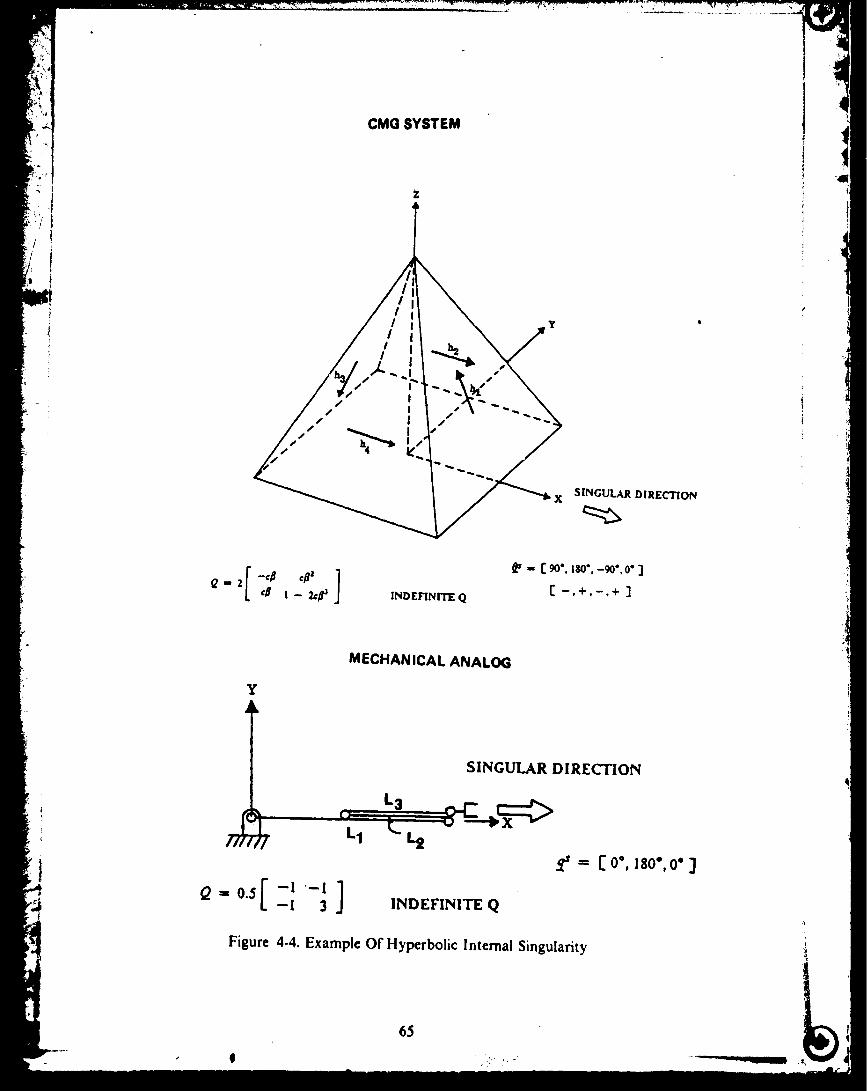
,.j

CMG SYSTEM

SINGULAR DIRECTIO/qX

¢

°

Qt2INDEFINITE Q

_,- C9o'.tso'.-9o'.o"3

C -.+.-.+ ]

MECHAN ICAL ANALOG

Y

I SINGULAR DIRECTION

Q = o.5[ -_-_ ]--I 3 INDEFINITEQ

Figure 4-4. Example Of Hyperbolic Internal Singularity

65

• • _7' 7"_ ..........

}4

_'! pie used in Figure 4-2. The singular configuration for the CMG system is defined by

the gimbal angles: 0 s = [ -90 °, 180 °, 90 °, 0 ° ].

The row-echelon form of the Jacobian and its corresponding null-space basis is

given by:

J

! 0 1 2c/30 1 0 --1

0 0 0 0 -l -2c/_

0 1

I 0

0 1

The Q matrix and its upper-triangular form are:

LII

t

'41

] =2ic ]Q = 2 c/J 2 2c/33 + 1 0 cfl 3 + !

The pivots are cfl and c[33 + !. Both are positive, thus Q > O, i.e. is positive definite.

This suggests that the singularity is of Elliptic ty'pe and is unescapable by null motion.

No null motion whatsoever is possible for this case, as earlier observed to be a proper-

ty of the Saturation singularity.

In the case of the manipulator, the singularity is defined by the joint angles:

_qS = [ 0 o, 0 o, 0 o ] The row-echelon form of tile .lacobian and its null-space basis

are:

-0.5 -0.5 1[ I 0"5 '"5 ] N = I ,}J = 0 0 0 0 !

66 ®

The Q matrix and its upper-triangular farm are:

o,[,1]1 3 Q = 0.5 0 8/3

The pivots are 3, 8/3. Both pivots are positive, and Q > 0. The singularity is therefore

Elliptic, and no null motion is possible.

4.6 MEASURE OF SINGULARITY

We have seen that the rank of the Jacobian matrix is an indicator of the singulari-

ty of the CMG system. This information can be used to detine an index, the singularity

measure m, which shows how close the CMG system is to being singular. In the litera-

ture, m' is also refered to as the CMG "gain" [15]. The dcrivation of the singularity

measure presentcd hcrc employs the Singular Value I)ecomposition (SVi)) of the Jaco-

bian matrix, which is given by:

J(O) = U_Z V r (4-11)

where U is a 3 x 3 orthonormal matrix

V is a n x n orthonormal matrir

[ oo ]V, ____ 1) 0"2 0 F 0 1

0 0 °',3

tr_ =_ 0 singular values

For a matrix to be nonsingular, all of its singular values must be greater than zero

[2], therefore the product of the singular values can be used as a singularity measure.

This is given by:

67

v

b,,(,;

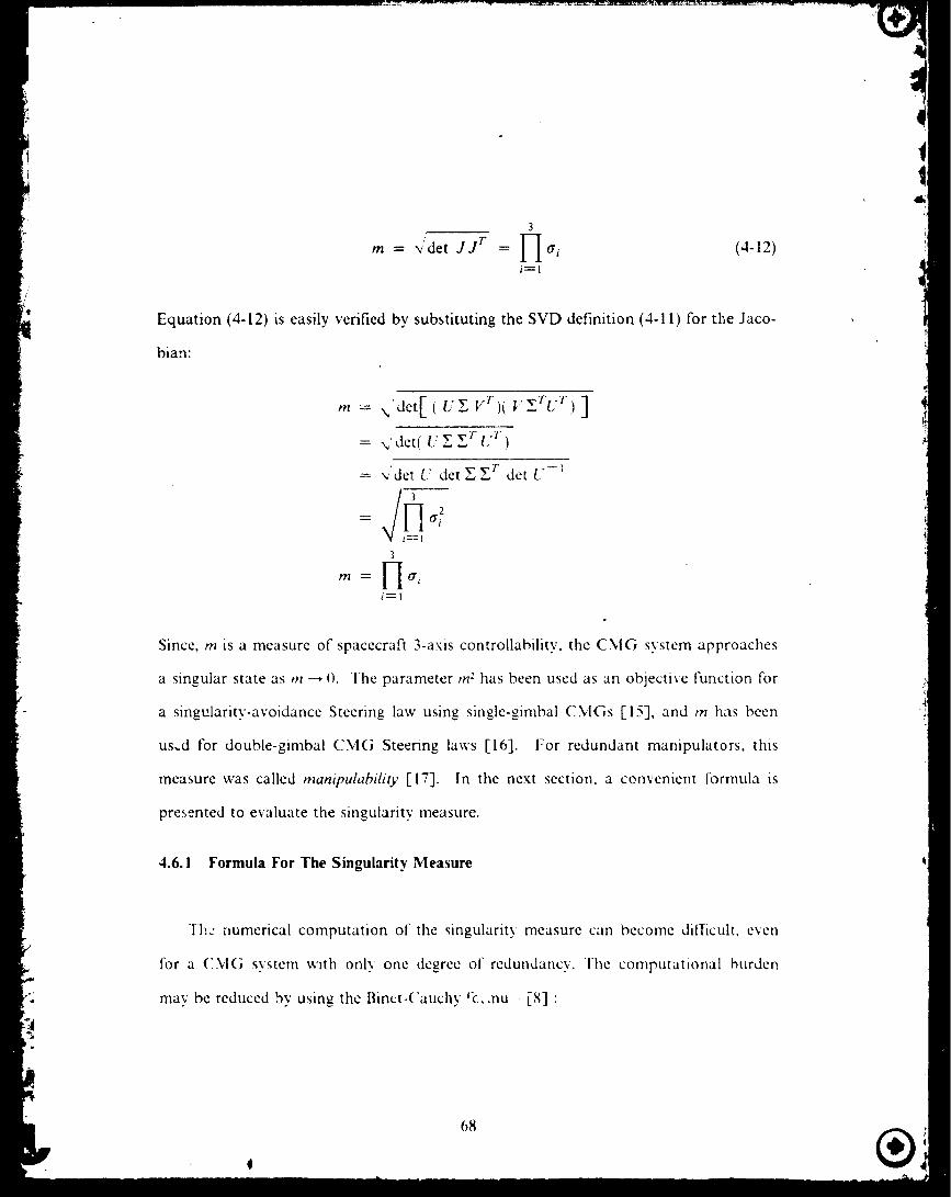
3

r [-Im = "v'det jjr = a; (4-12)

ial

Equation (4-12) is easily verified by substituting the SVD definition (4-11) for the Jaco-

bian:

/

,-,,= ,, det[ ( u_ v")i _Uc _) ]

= ,,'det( UZZrU r)

= ,,det U detEE r det U -_

3

i=l

Since, rn is a measure of spacecraft 3-axis controllability, the CMG system approaches

a singular state as m--, O. The parameter m: has been used as an objective function for

a singularity-avoidance Steering law using single-gimbal CMGs [15], and m has been

us,d for double-gimbal CMG Steering laws [16]. For redundant manipulators, this

measure was called manip,dability [17]. In the next section, a convenient fbrmula is

presented to evaluate the singularity measure.

4.6.1 Formula For The Singularity Measure

ll_c numerical computation of the singularity measure can become difficult, even

for a CM(i system with only one degree of redundancy. The computational burden

may be reduced by using the Binct-Cauchy rc.,nu [8] •

68

/'!

m

x(s- 2)3_

, N > 3 (4-13)

where 3/1i = ( N ) distinct Jacobian minors of order 3

For the Pyramid mounted 4-CMG system, the measure can be written as:

m = ,( + .+t++ + .+t# 1414)

The evaluation of the singularity measure is much simpler by this formula, since

the order 3 minors of the Jacobian matrix are dimensioned smaller as well as having

simple entries than the square matrix formed from ( J jr ). Since this formula exprcsscs

the measure in terms ol_ all distinct minors of order 3 which are extractable from tile

Jacobian, we can see from (4-14) that individual minors can be zero, (implying loss of

three-axis controllability for the corresponding sub-system of 3 (.'MGsl while the sxs-

tern as a whole remains non-singular.

A new measure of distance from singular points was recently proposed tbr redun-

dant manipulators [18]. This new measure is defined in terms of the product of non-

singular Jacobian minors. Since the minors represent the relative tblding of all

sub-groups of links, this measure reflects the number of relatively unfolded (non-coli-

near) groups of links remaining ta the manipulator system. This approach can analo-

gously be used in CMG Steering lairs, i lowever, since keeping the product of minors

non-zero prcc!udcs the switching of solutions (or linkage configuration) it is felt that

this approach is not appropriate for (?MG Steering laws.

69

This switching of solutions is determined by the singular minors, that is gimbal

angles for which .14, = 0, define the boundary between one form of joint configuration

and another form. In nonredundant systems, this boundary is defined by det(J) = 0.

This fact can be most easily understood by refering to the planar 3-1ink manipulator

(introduced in Chapter 2) in Figure 4-5, which shows the transition from one joint

configuration or closure (A) to another closure (C) through the switch configuration

(B) while the total system is nonsingular through the switch. It is seen that the switch

boundary occurs when links #2 and #3 are colinear, which implies that

M3 = 12_'2_31 = 0 at the boundary, while the other two minors are nonzero. This

switching is undesirable in manipulators because it leads to repeatability problems. On

the other hand, in CMG systems this switching is desirable for singularity avoidance.

it/

i,r

_f

?'t

J

,Ib •'% •

Figure 4-5. Transition Between Two Joint Closures Via Singular Minor

7O

/

4.6.2 Singularity Measure And Null-Space Of Jacobian

We have seen that the singularity measure of the Jacob(an can be expressed in

terms of its minors. It has also been shown that the Jacob(an null-space can likewise be

expressed in terms of the minors. What then, is the relationship between the two, if

any? In order to examine the relationship, we will use the 4-CMG system as an exam-

ple (what follows is actually valid for any system with one degree of redundancy). The

definition below provides some illumination:

Definition: For any non-singular real matrix J of dimension m x (m + 1)

where

det( J Jr) = I v 12

v = Jacob(an null-vector

Proof: (;sing the notation of Chapter 2 and the Jacob(an mutrix of the 4-CMG sys-

tem. we can write:

71

Armed with this definition, the null-vector of the Jacobian can be better under-

stood; this understanding will be vital in the design of the Steering law. The fundamen-

tal attributes of the null-vector, its magnitude and direction, for non-singular systems

of single-degree redundancy can be summarized as follows:

Magnitude Of Null-Vector: The magnitude of the null-space basis vector is identical to

the singularity measure, m, thus is directly related to the nearness of a singularity.

Direction Of Null-Vector: The direction of null motion is defined by the non-zero dis-

tinct minors of order 3 extractable from the Jacobian matrix. The availability of null

motion from each CMG is also determined by these non-zero minors.

The above statements dictate that the amount of null motion available from each gim-

bal is governed by both the singularity measure and its corresponding minor. On the

other hand, the possibility of extracting null motion from each CMG is determined

only by the value of the corresponding minor.

72

_! ,..2 _.

CHAPTER 5

KINEMATIC REDUNDANCY RESOLUTION METHODS

5.1 GENERAL SOLUTION METHODS

In this chapter, various torque-input Steering laws will be reviewed, and their per-

formance evaluated. Alternative methods of singularity avoidance will also be pro-

posed, and their behaviour likewise examined. The results of Chapter 4 will be used

extensively to evaluate and understand the performance of the different Steering laws.

It will be shown that existing singularity avoidance methods do not avoid Elliptic type

internal singularities.

Kinematic methods of redundancy resolution require the solution of an undcrdetcr-

mined system of linear simultaneous equations (the torque equation) involving the

instantaneous Jacobian matrix of the CMG system.

These methods are refered to as local, because they yield gimbal rate solutions to the

instantaneous torque request. Redundancy is also resolved instantaneously, based on

some criteria that hopefully steer the gimbal angles away from internal singular config-

urations while simultaneously satisfying the torque request, r_. Local methods have the

advantage that real-time implementation is readily feasible.

The general solution to (3-6) was shown in Chapter 3 to be formed from the

Moore-Pcnrose pseudoinverse and any homogeneous solution. This form can be fur-

ther classified into the following three categories:

73

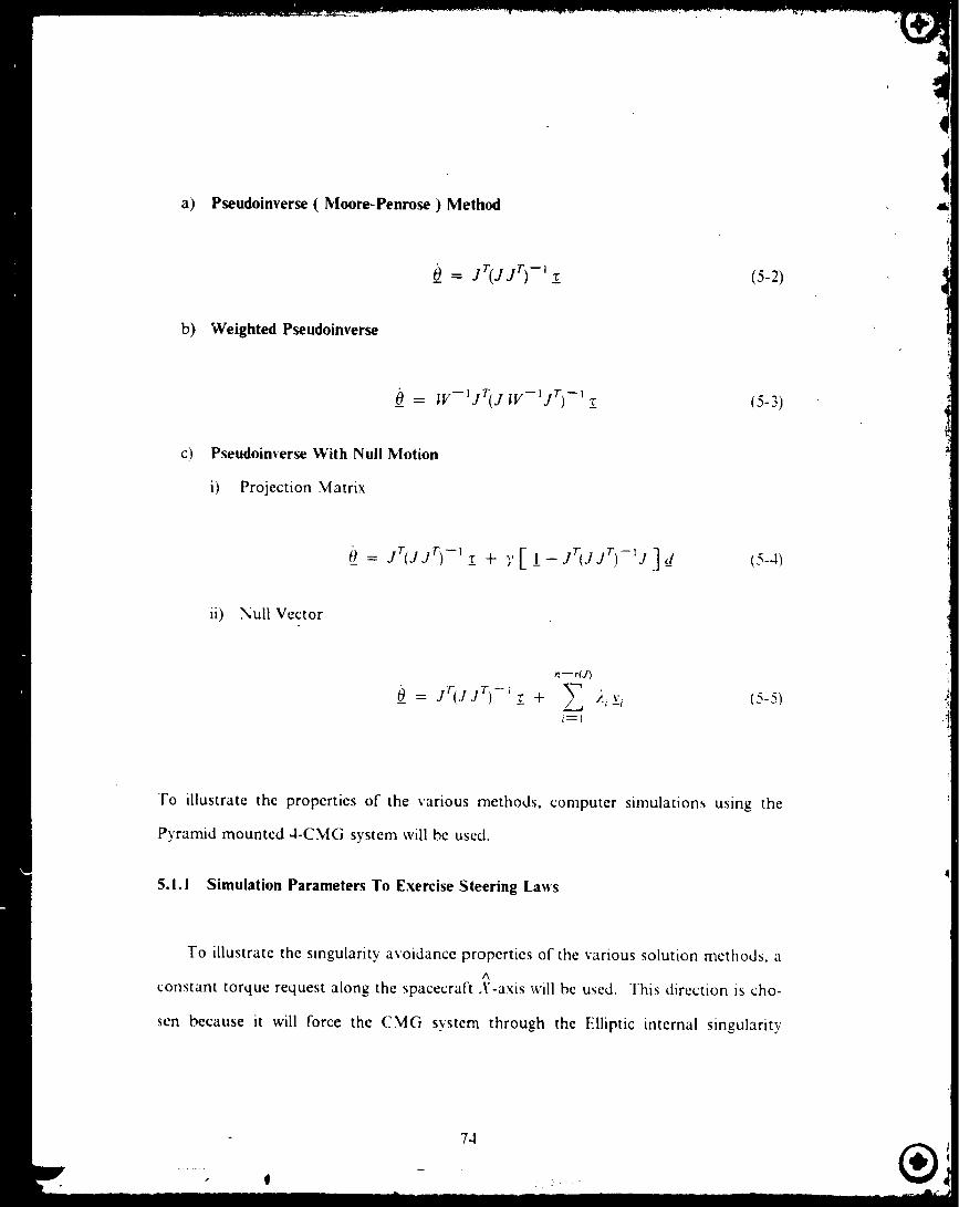
a) Pseudoinverse ( Moore-Penrose ) Method

= JT(JJS-I ! (5-2)

b) Weighted Pseudoinverse

= W-IjT(j IV-IjT) -I z" (5-3)

c) Pseudoinverse With Null Motion

i) Projection Matrix

O_= jTIjJS-' __+ r [ ! - JqJ J')-' J ] <! (5-4)

ii) Null Vector

n--r(J)

_5-5)

To illustrate the properties of the various methods, computer simulations using the

Pyramid mounted 4-CMG system will be used.

5.1.1 Simulation Parameters To Exercise Steering Laws

To illustrate the singularity avoidance properties of the various solution methods, a

Aconstant torque request along the spacecraft X-axis will be used. This direction is cho-

sen because it will force the CMG system through the Elliptic internal singularity'

7d

r_

which was analy'zed in Chapter 4. Since the Elliptic singularity represents the worst

type of singular configuration, it can be used as a measure of the singularity avoidance

capability of the particular method used in the Steering law. Also, the torque request

is aligned with the singular direction, which represents the worst possible combination.

It should be noted that non-degenerate Hyperbolic internal singularities can be avoided

by any of the above methods; this will be shown by computer simulation.

During tile course of the computer simulations, it was found that the method used

to calculate the pseudoinverse could affect the gimbal angle trajectories. The first meth-

od which was used, numerically evaluated the pseudoinverse using symbolic expressions

for the adjoint of the square matrix (J JO and its determinant. This square matrix is

ideally symmetric, however, during computation it was observed that there were slight

discrepancies between the off-diagonal terms due to truncation errors. For this reason,

the dyadic form of (j jr) was used instead (as in [1]) to obtain a closed form solution

for the torque producing gimbal rates. This solution is given by:

Or - ! ( ._t

Or_ 12 { -_t, I J,_j___r[ - ._I21j,_J__-rl + ._t_lj:__J___1}m

0 r _ 12 {._t, IJ__J2_ _r I - ._t_ IJ,_j_ _r I - ._t_IJ:_A r I im

Or _ 12 {M2 I J,_ -, I + .U,[J,_J3_ -= I + I;,..J,_-=I}

where ._l_ = Jacobian mm,,r.s oj',,rder 3

Of = l;_rqtw [,r,,du,:m_.q, imhal rates

This approach was found to yield more accurate results than the _xmboltc m_erse.

75

The CMG dynamicswere integratedat a simulation interval of 0.01sec,unless

otherwisestated. Thegimbalrateswereintegratedusingtheroutine DVERK from the

IMSL library, which performsa fifth-sixth order Runge-Kuttanumeric integration.A

tolerancevalueof 0.0001wasused. Programswerewritten in doubleprecisionFortran

77.Thetorquerequestand angularmomentummagnitudesweresetequalto unity (i.e.

I r_.I = 1),and no rate limits wereenforced.The applied torque request vec-h = 1,

tor was:

['Jt= 0

0

The initial gimbal angles for all simulations were each set to O.

5.2 PSEUDOINVERSE ( MOORE-PENROSE ) METHOD

The properties of this method were discussed in detail in Chapter 3, thus will not

be repeated here. It has been shown [19] that this method can generate gimbal angle

trajectories that pass arbitrarily close to singular points in gimbal angle space, therefore

this method cannot be used by itself to avoid singular states.

From the simulation results given in Figure 5-1 this t_act can be easily seen. The

singularity measure m ( SQRT(DET(JJT)) ) nears zero as the X component angular

momentum (tlX) approaches 1.15, indicating that the CMG system is singular. The

singularity measure is non-zero as ftx passes 0.85. indicating that the l lyperbolic singu-

larity analyzed in ('hpater 4 is avoided. This is the method by which the degeneracy of

the I lypcrbolic singularity is currently determined. The inner product of tile torque

76

". g

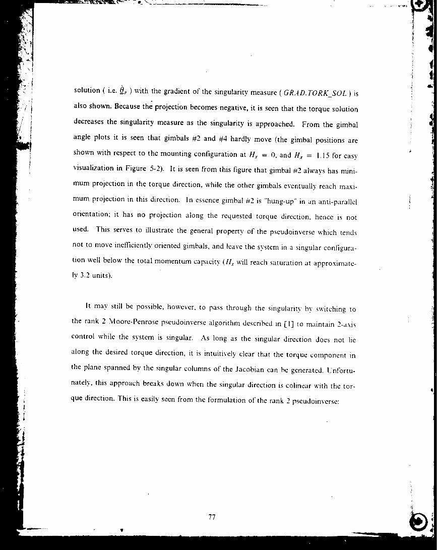
i ij i; i

.i

solution ( i.e. O__p) with the gradient of the singularity measure ( GR,4 D. TORK_SOL ) is

also shown. Because the projection becomes negative, it is seen that the torque solution

decreases the singularity measure as the singularity is approached. From the gimbal

angle plots it is seen that gimbals #2 and #4 hardly move (the gimbal positions are

shown with respect to the mounting configuration at Hx = O, and Hx = 1.15 for easy

visualization in Figure 5-2). It is seen from this figure that gimbal #2 always has mini-

mum projection in the torque direction, while the other gimbals eventually reach maxi-

mum projection in this direction. In essence gimbal #2 is "hung-up" in an anti-parallel

orientation; it has no projection along the requested torque direction, hence is not

used. "lhis serves to illustrate the general property of the pseudoinverse which tends

not to move inefficiently oriented gimbals, and leave the system in a singular configura-

tion well below the total momentum capacity (Ilx will reach saturation at approximate-

ly 3.2 units).

tl

!I

1

It may still be possible, however, to pass through the singularity by switching to

the rank 2 Moore-Penrose pseudoinverse algorithm described in [1] to maintain 2-axis

control while the system is singular. As long as the singular direction does not lie

along the desired torque direction, it is intuitively clear that the torque component in

the plane spanned by the singular columns of the Jacobian can be generated. Unfortu-

nately, this approach breaks down when the singular direction is colinear with the tor-

que direction. This is easily seen from the formulation of the rank 2 pseudoinverse:

77

-!!

i

- 1198 ---_-'--';---T --_ .... _---'r---r----_0, .12 ,24 .36 .48 ,6 ,72 ,84 ,96 i,08 i,2

i.270 .... HX (ANG MOM)• i • i

.,

-,1270 , .la ,14 ,_6 ._8 .'_ ,;z ._4 ._6i,b8_a2.395 GRAD. TORK_S, OL

-26,58 i , , l , i ,O, ,12 ,24 ,36 ,4.8 ,6 ,72 ,84 .96 1.08 i,2

Figure 5-1. Simulation Results For Mc;ore-Penrose Method (Part 1 of 2)

0,16 T,HETA, i ,(RAD)

-i,70' i i l i,24. ,4.8 ,72 ,96 I,_.

1,7 THETA 3 (RAD)I ; | I

-.i70, .24 .48 .72 .96 i,2

0,47

d

I0d

X

THETA 2 (RAD)

I0d

X

31 THETA 4- (RAD)

-5'30, . 4 .48 .72 .96 i.Z "3'to, .24 .¢8 .72 .96 i.Z

Figure 5-1. Gimbal Angles For Moore-Penrose Method (Part 2 of 2)

78

/

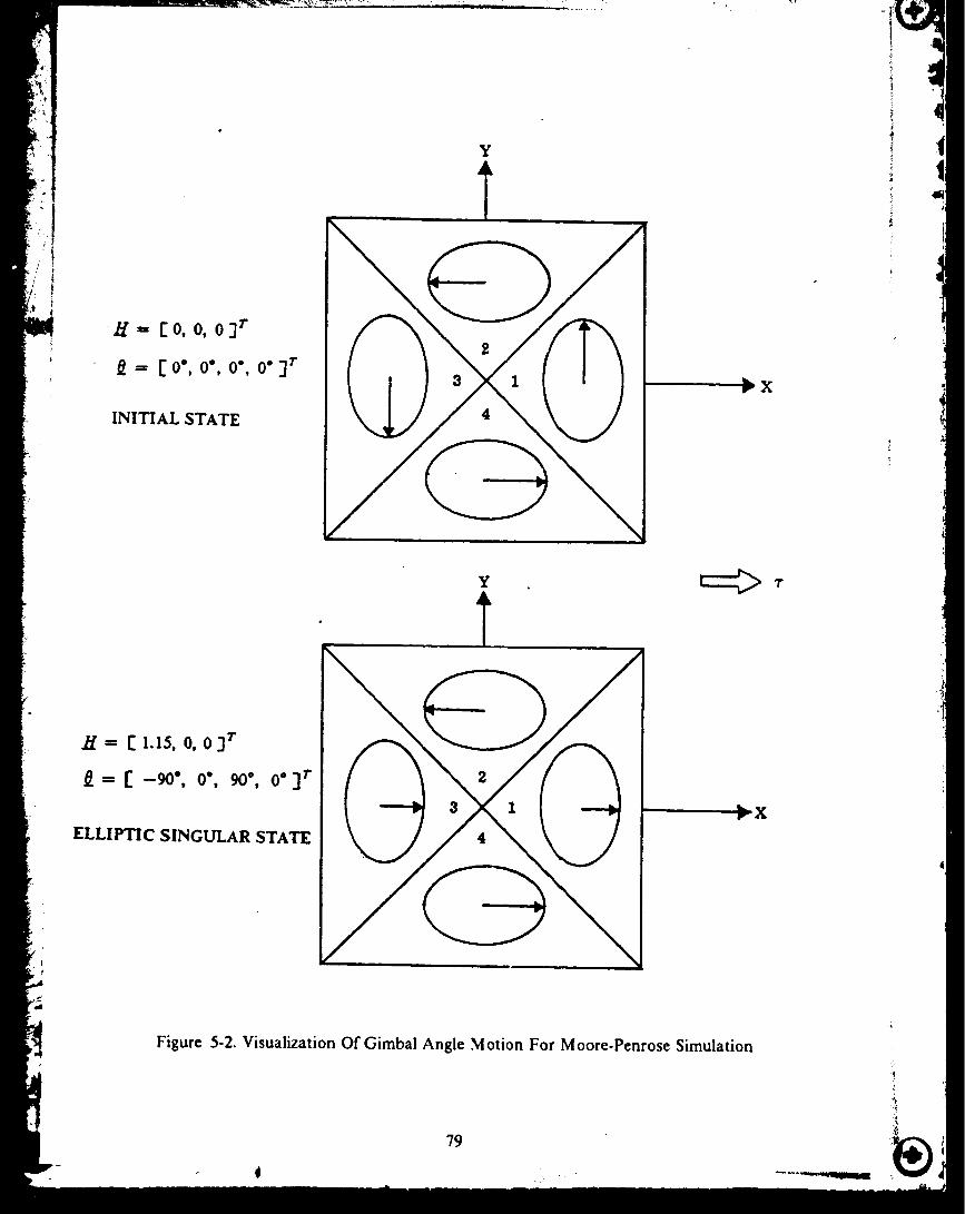
/ i!

' i

•/f ffi [o. o, o3 r

- [o', o', o°, o°3 r

INITIAL STATE

r-X

//ffi [ 1.15, o. o 3 r

0 ffi [-9o', o', 9o', o']r

ELLIPTIC SINGULAR STATE

Figure 5-2. Visualization Of G imbal Angle .Motion For M oore-Penrose Simulation

79

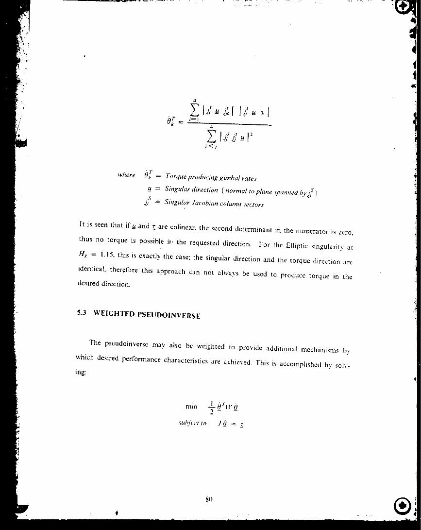
4

Of=4

i<j

where 0 T = Torque producing gimbal ratea

u = Singular direction ( normal to plane spanned b),_ s )

.SJi = Singular Jacobian column vectors

It is seen that if_u and _z are colinear, the second determinant in the numerator is zero,

thus no torque is possible it_ the requested direction. For the Elliptic singularity at

H, = 1.15, this is exactly the case; the singular direction and the torque direction are

identical, therefore this approach can not always be used to produce torque in the

desired direction.

5.3 WEIGHTED PSEUDOINVERSE

The pscudoinverse may also be weighted to provide additional mechanisms by

which desired performance characteristics are achieved. This is accomplished by solv-

ing:

rain ±oqvO

sut,je,'t to J 0__= z

|

The weighting matrix _V must be positive definite. It is seen that the Moore-Pcnrose

(M-P) method is obtained by setting the weighting equal to the identity matrix 1.

L

!b•

b",P. tii

The properties of this method are essentially the same as those of the M-P method

as long as _F = kl For this case, the particular solution 0__pis orthogonal to the

homogeneous solution _-H-Otherwise, this property is not preserved, and this new sol-

ution can be expressed as a combination of the M-P inverse and a homogeneous term.

Assigning different values to the diagonal elements of W causes the participation afa

particular gimbal with lower weighting to be favored more heavily in the solution; une-

qual weighting of gimbal rates thus enforces high-authority low-authority partitioning

of gimbal activity. This method may be used to reflect the energetics ofa system

(thereby minimizing energy}, which would make it a dynamic rather than a kinematic

method. An example of this would be using the inertia matrix of a manipulator as the

weighting matrix in order to minimize system kinetic energy. This approach has been

used in robotic applications, however it did not offer any improvement over the M-P

inverse as far as singularity avoidance is concerned [20].

From the previous pseudoinverse simulation results, it was noted that gimbal =2

was essentially not moved. To encourage the motion of gimbal #2, a time varying

diagonal weighting matrix was attempted. The intent was to reduce the penalty of inef-

ficiently placed gimbals, thereby hopefully encouraging their movement. Correspond-

ingly, an,,' maximally projected gimbals were weighted with a higher cost to attenuate

their participation. 1he diagonal entries o['the weighting matrix thus become:

81

®

,!

J

m

,

!

where wo = Initial weighting

CO = Aqultiplier

The results of this approach are shown in Figure 5-3. The parameters that were used

are w0 = 1, Co = 2 . The effect of the weighting matrix on the determinant of the

square matrix J W-_J r ( SQJ DET), is seen not to prevent it from becoming singular.

It is seen that the singularity at Hx = 1.15 was still not avoided. From the weighting

plots it is seen (as expected) that gimbal _2 always has the smallest cost, while the cost

on gimbals #1 and #3 continuously increased as they approached maximum projection

on the torque direction. Comparing the gimbal angle plots of this approach with those

of the M-P inverse, it seen that they are essentially identical. Although this method

may hold prmruse in re-partitioning the use of different gimbals if off-diagonal terms

were used in the weighting matrix, it has been shown to be ineffective in avoiding sin-

gular states. Since this solution can be written in terms of the M-P inverse and an

appropriately chosen homogeneous solution, it will not be pursued thrther.

5.4 PSEUDOINVERSE WITH NULL MOTION

We have seen that the pseudoinverse solution bv itself does not provide any singu-

larity avoidance ['or l.lliptic singularities. Since the homogeneous solution has no pro-

jection on the row space of (3-6), i.e. produces no torque, it can be used to shape the

complete solution and hopefully provide a means of singularity avoidance. [he steer-

ing problem then reduces to picking a vector in the null-space of the Jacobian such

that all internal singularities are avoided. lhe addition of null motion thus is to steer

the gimbal angle trajectory to an alternative non-singular contiguration corresponding

82

I

1,2 SQRT(DET(JJT) ) 1.3_ , _.J D,ET

-.12- - - -_-- - "T- -.24 .48 .72 ,96 1.2 't30, .24 .48 .72 ,96 t,2v.

3.6 Wi W.EIG.HTING 3.6 W3 W.EIG,HTING ,

l.i W2 WEIG,HTING 5.5 W4.... WEIGIHTIIG 'I

O. .24 . 48 , 72 ,96 .2 O, .24 . 48 .72 .96 i. 2

Figure 5-3. Simulation Results For Weighted-Pseudoinverse (Part 1 of 2)

,-f

0,16

-1.8 i I I JO, ,24 ,4B ,72 .96

-6, 2

,2

1.7 THETA 3 <RAp)

-.t7 "1- ] - r " '1- 'O, ,24 .48 .72 . _6 l, 2

61 _THETA 2 (RAD) 0.39

m

m

_m0, .24 .48

THETA 4- ( RAIJ )

I -0

m

dva m

-4.3.72 . _6 t. 2 O, ,24 .4B . 72

_L__,$6 i ,2

Figure 5-3. Gimbal Angles For Weighted-Pseudoinverse (Part 2 or 2)

83

to the singular momentum state. In Chapter 4, it was shown that not all neighbor-

hoods of internal singularities can be escaped using null motion to reconfigure the

momentum linkage; this method is effective only as long as the gimbal angle trajecto_'

does not approach neighborhoods of Elliptic or degenerate IIyperbolic singularities. It

will be demonstrated that the addition of any class of null "notion does not completely

address the singularity avoidance problem.

5.4.1 Projection Matrix

One way of obtaining a _ector in the null-space of the Jacobian _s by using an

operator that projects an arbitrary' n-vector inte its aull-space. One such operator, the

Projection matrix, is given by:

P = [ - J q,l J r)- 1 j

For a singularity avoidance control law, all that remains is to pick the projection

vector ;'d as in (5-4). In [19], it is shown that arbitrary gimbai angle trajectories

which do not pass through a singular configuration may be generated using this meth-

od bv an appropriate choice of','d. This result requires that one choose a priori a sin-

gularity free gimbal angle trajectory, and also select a projection vector _hat can

recover or generate this trajectory. Normally, such a traiectory is not known belore-

hand; the generation of such a trajecto_ becomes the design objective.

The usual approach to smgularity avoidance is to choose tins projection _ector

such that a scalar perlormance index (such as the singularity measure_, is 'optmu/ed.

®

One way of accomplishing this is to maximize a scalar performance criterion p (0_) by

choosing _das in [16]:

4r _ Op (0) (5-61

These types of procedures are usually refered to as gradient methods. Since, p = Cjr_0_,

we use (5-4) to obtain:

P = _t'r.]liJ Jr)--1! + 7 dr[ I_ - jT(j jl')-I j ],__/ i5-7)

The second term in the right-hand side is non-negative because the projection matrix is

positive semidefinite [2], and contributes to an increase in the _alue of p. One way of

choosing the scalar '/is to maximize p (u = 0) subiect to upper bounds on gimbal rates

[16]. The singularity ,;_:.'asure, m was chosen as the performance index. [t should be

noted, however, that the singularity measure is not a monotonic function of the gimbal

angles, thus instantaneously maximizing this ['unction can lead to local extrema of the

measure. It is shown in [15] that this method does not avoid singular states because

the system is controlled to stay at the local maximum, and there exist trajectories of

local maxima which nearly extend to singular points. Another wax of expressing th_s is

that the right hand side of(5-7_ can be negative and may dominate p, thus resulting in

a net decrease in the value ofp. This phenomenon will be examined [hrther in the next

section.

It is also mentioned in [ll]txithout an} parttcular relcrcnces_ that gradient meth-

ods using a perlbrmance index

qi:'

1P- 2

m

have been tried unsuccessfully by several authors. It was suggested that the reason for

this was that the determinant was not sufficiently sensitive to allow appropriate null

motion be added in time to avoid close encounters with internal singularities.

5.4.1.1 Indirect Avoidance Control Law

Another way of choosing the projection vector can also be found in [11]. This

method, called the indirect avoidance law, relies on the observation that internal singu-

larities can be avoided in most cases by merely steering towards the Saturation sing_-

larity associated with the instantaneous torque request. This method was succcssfull in

avoiding internal singularities for a 6-Pyramid CMG system. Since we have sccn in our

simulations that gimbal =2 was persistently "hanging-up" antiparallel to the torque

request tbr the M-P inverse, this method seems to provide a mcms of encouraging this

gimbal to move. The projection vector for this approach is defined _s:

_a= a0_ = 0_

,." -y Op)' = A A -

X • V

"f .:

i, i

where'AO ^

_sat -- 1 Ji " 12= tan A

hi 0 A.12

Au = unit(z_)Az = unit(PA_)

Ay = unit(AO)Ax = unit( O__p)

P = Projection matrix

The indirect avoidance law was implemented Jn simulations of the 4-CMG system with-

out limiting the amount of null motion. The projection matrix was numerically calcu-

lated using the symbolic adjoint of (j jr). The simulation interval was 0.005 see., with

a final time of I.IS sec. The results of the simulatio_t .are shown in Figure 5-4. It is

seen that the Elliptic singularity is again not avoided since m still approaches zero at

tlx = 1.15. The projection of the null vector, __-,on the gradient is seen to go to zero

near the singularity, thereby rendering any null motion ineffective in avoiding it. From

the gimbal angle plots, it is observed that both girabals =_2 and _4 move slightly, but

not sutficiently to "'un-lock" gimbal _2.

i1

l

5.4.2 Null Vector

The Jacobian null.space basis vectors can also be used to Form the null-vector.

With this approach, only tile scalar weighting factors remain to be determined. It

should be noted that as the redundancy of the system increases, the dimension of the

null-space also incrt'ases, which complicates the choice of these factors. [:or the case of

four CMGs and _J nonsingular Jacobian matrix, the null-space dimension is one. thus

null motion is restricted to a line. All that remains m this case is to choose the magm-

87

SORT(Clef (JJT))t,t98 .........

-.i198 ---_---7---r---, .... L -TO. .12 ,2'; .36 .48 .6 .72 .84 ,96 1.08 1,2

HX (ANG NON)t,270 . . . . . ..

-.laTO .ta ._.4 ._ .J,8' ,_ ._a ._4 ._ _.b8 _,z0.09¢2 . (BRAD. NULL_V, EC , , ,

-. t235 !t

0. .12 .26 .36 .48 .6 ,72 .84 .96 t.08 t.2

1

Figure 5-4. Simulation. Results For Indirect Avoidance Law (Part I of 2)

0.16 THETA 1 (RAD) i,7 THETA, . 3 ,(RAD, )

-i 7 0 t - i70.' . ,24 .68 .72 .96 1,2 ' ,24 .68 .72 ,96 i, 2

0,04 0,ii THETAI lT,HETA 2 (RAp)

I

l l I -.060 ' J i-, 04 O. .24 .48 .72 .96 i. 2 .24 ,48

4- (RAD),

I I

I I,72 ,96 t, 2

Figure 5-4. Gimbal Angles For Indirect Avoidance Law (Part 2 of 2)

88

®

rude and direction in which null motion is applied by using a single scale factor. The

homogeneous solution can then be written as:

.O-H= 2v

7•if!

.i

,!

One method of choosing the scale factor for a 4-Pyramid CMG system is given in

[15]. This approach, called the maximum gain method, involves steering the null

motion towards the point of maximum gain, ,n 2. This approach is global in the sense

that the direction of r_ull motion is oriented towards the point of global maximum gain

in gimbal angle space, as obtained from a look-up table which is generated by off-line

calculation and reduced to a small size by taking advantage of the symmet_' of this

particular configuration. This method also requires the location of all Elliptic type

internal singularities to be determined in order that gimbal angle trajectories ahvaxs

avoid the neighborhoods of these singularities. This is accomplished by modit'ying the

gimbal rates.

The null vector strategy was applied in two different singularity avoidance laws.

Both of.these methods exploit the relationship derived in Chapter 4 between the null-

space of the Jacobian and the singularity measure (or gainS. These methods are:

a) Gradient Method

b) Inverse Gain Method

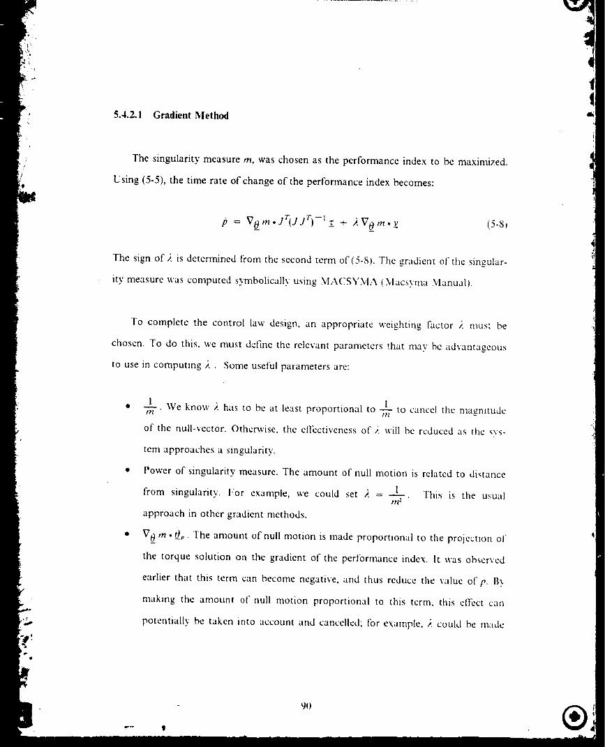
U

5.4.2.1 Gradient Method

The singularity measure tn, was chosen as the performance index to be maximized.

Using (5-5), the time rate of change of the performance index becomes:

i, = vo_m. JrIJ jr)-, __+ _.vo m. (5-Si

1qt!

i

_q

_J

The sign of ). is determined from the second term of(5-Sk The gradient of the singular-

ity measure was computed symbolically using MACSYMA (Macsvma Manual).

,',_,

_O'!

To complete the control law design, an appropriate weighting factor ). must be

chosen. To do this, we must define the relevant parameters that may bc advantageous

to use in computing ,;.. Some useful parameters are:

. 1• __lrn We know ,;. has to be at least proportional to -7k" to cancel tile ma_,nitude

of the null-vector. Otherwise. the effectiveness of ,;. will be reduced as the s\s-

tern approaches a singularity.

• Power of singularity measure. The amount of null motion is related to distance

from singularity. [:or example, we could set ,_. -- 1 This is tile usualm"

approach in other gradient methods.

• V 0 m._0_p. The amount of null motion is made proportional to tile project,3n of

the torque solution on the gradient of the performance index. It was observed

earlier that this term can become negative, and thus reduce the value o/'p. Bx

making the amount of null motion proportional to this term. this elt'cct can

potentially be taken into account and cancelled; tbr example. ,;. could be made

1

proportional to this term whenever it is negative. This scaling has not been uti-

lized in other gradient methods.

V 0 m. v. The amount of null motion is made proportional to the projection of

the null-vector on the gradient of the performance index. This term expresses

the possibility of affecting the index through null motion; if this term is small.

the effectiveness of null motion is reduced, regardless of how it is determined.

Taking into account all of the above criteria, the gradient method is forn_ulated

using a weighting factor that includes a a contribution from each parameter:

W Ortt'V [ V OmoJT(JJT)-I ! [). = - - (5-9)

2r?l

This approach is somewhat unique; of the gradient methods published in tile literature

[il], [15], all lack at least one of the four criteria mentioned above.

Simulation results ['or this method are shown in Figure 5-5. It is seen that the

Elliptic singularity is still not avoided. The reason becomes evident if we look at the

plots o[" the null-constant ,;. ( NULL CONSI'NI') , and the gradient projection on the

null-vector { GRAD.NULL VEC). It is seen that the null-constant remains essentially

zero up to the singularity. This is because the null-vector has very small or no projec-

tion on the gradient at this period, thus no null motion was added. This simulation

then is identical to using the M-P inverse by itself l.ooking at the gimbal angle plots.

we see that gimbal _2 does not move. just as m the M-P inverse method.

_)I

1,2 SORT (DET (JJT) )

(,

-I- -.1 - -ii 't20, ,24 ,48 ,72 .96" t.2

1.3 HX (.ANG r,lOl--1)i !

-,t3 .I I i . I_, ,2.4 ,48 ,72 , _6

NULL CONSTNT

.2,$ . 48 . 72 .96 i. 2

GRAD, NULL_VECw B w i

I I , | I .,24 ,48 , 72 ,31_

Figure 5-5. Simulation Results For Gradient Method (Part l of 2)

0,16

-i,7

0,i3=i

-

I -0d

X -

-1.4O.

THE TA 1 (RAD)

), . I I I . I..24 . 48 . 72 .96 ,2

i,7 .. T,NETA, 3 ,(RAp)

- t70, . J I.' .124 .148 .72 .96 1.2

THETA 2 (RAD)I I I " I

i

I I I. I,24. ,48 ,72 ,96

.a4

d

x

-9.5,2

T FIETA. 4. ,(RAp)

- l, j" I j-

.24 . ,_8 .72 .96 1.2

Figure 5-5. Gimbal Angles For Gradient Method (Part 2 of 2)

92

The Moore-Penrose pseudoinverse is actually seen ira this case to directly generate

a gimbal angle trajectory of locally extreme m when commanding momentum to

increase from zero along the X-axis (as shown in this example). This illustrates a gener-

al defect of locally-optimal procedures which was mentioned previously; they tend to

lock into trajectories of locally maximum gain which can actually lead into singular

configurations.

1[!

To overcome this shortcoming, another form of the gradient was tried, where the

null-on-gradient projection was replaced by its sign. This is given by:

L ign(VOm" ) l Vom"f'l J - ' [2 = - - !5-1o)

2t7"/

Simulation results for this approach are shown in Figure 5-6. It is seen that the singu-

larity is still not avoided. At the end of the simulation, the system is actually trapped in

a near-singular configuration about the Elliptic singularity'; it does not attain the exact

singular configuration, as seen from the very small (but still finite) value of m. The

null-constant in this case is almost always non-zero and the null projection onto the

gradient also becomes substantially non-zero, indicating that a different gimbal angle

trajccto_ was generated here than the previous gradient n_cthod. In this case, the null

motion (with magnitude now governed by the torque projectien and singularity meas-

ure) is added increasingly to the solution as the torque request pushes r.he system

toward the sitagular state, l.ooking at the gimbal angle trajectories, it is seen that gim-

hal _2 moves about 15° during the period when the null-projection is non-zero; howev-

er this is not sutficicnt to avoid the singular state, and it is pulled back again again by

the torque requcst. The gimbal angle plots tbr this example also illustrate how gimbal

93

#4 hasto correspondinglymovein order to balanceoff-axistorquesand "unlock" gim-

bal #2.

5.4.2.2 Inverse Gain Method

The previous examples indicated that dynamically manipulating the direction of

null motion to instantaneously maximize controllability has been ineffective in avoiding

singularities. This is due to the tendency of tangent-based methods to lock onto locally

optimal gimbal angle trajectories that can lead toward singularities, as stated earlier.

Based on this observation, a non-directional approach to singularity' avoidance was

tried, where the direction of added null motion was not specified, null motmn was

introduced in whatever direction the positive null-vector pointed; no sign factor was

imposed. This was accomplished bv choosing the weighting factor to include only a

contribution inversely proportional to _he sixth power of the singularity measure:

6t?/

l-he reason For this choice is detailed in the following argument. It was shown in

Chapter 4 that the null-vector, _vcan be written as:

!|J

!1

_..&

AV --'= ttl '9

A .

where v _s the unit vector in the direction of the null-vector. As discussed for the gradi-

ent method, the magnitude of the null vector is cancelled by dividing it with m . null

motion is thus added in the positive null direction, and the amount is proportional to

!_!__ Although this approach has the advantaae that it does not constrain null motion??lS

to always increase the singularity measure (this can avoid local optimum lookup, as

" t

i.2 .=,QRT ( DET (JJT) ) 0.16.

....11-' t'2 0, ,28 ,56 ,84 1,12 t,/_

!

[. ¢

GRAD, NIJLL_VEC

_28 J L i•56 .84 i.12

GRAD, TORK_SOL

I I 1 I•,28 ,56 , 84 i, 12

HX (ANG MOM) 2.3,

_.- ?;8' ._5_,'a_....1'._2 .4 . ,.4

,i

Figure 5-6. Simulation Results For Second Gradient Method (Part 1 of 2)

t,7, THETA 3 , ,0,15 THETA 1 ,(RAp) (RAI))

-,t7"t'70, ,28 ,56 .86 l,t2 .4 O, ,28 ,56 ,84 , ,4

0.25 -

II

-,06O,

THETA 0,07 THETA 4 (RAD)I I I I I I

2 (RAD)

! !

.86 i,i2 - 360,' ,28 .56 .84 i.t2 i,4

Figure 5-6. Gimbal Angles For Second Gradient Method (Pan 2 of 2)

95

,,i encountered in the gradient method), this approach has two potential shortcomings.

These are:

./ i a) null motion is added without regard to whether the performance index can be

4

instantaneously affected by null motion. The indicator for this situation is:

Vom.v = 0

b)

Even though null motion may not instantaneously increase the singularity mea-

sure (as dictated by the above situation), null rates of arbitraD' magnitude may

still be calculated and added to the solution.

Since the direction of null motion is not prescribed, it may actually decrease the

magnitude of the singularity measure; thus inadvertantly steering towards a sin-

gularity.

From simulations using different exponents on m, it was noticed that increasing the

exponent in the control law tended to increase the minimum value of m encountered

during the simulation, thus reducing peak torque producing gimbal rates. This can be

explained by the fact that increasing the exponent "flattens out" the m trajectory, when

m < 1 . Tb," effect is to anticipate the singularity earlier than with the control lax_s

using smaller exponents; the net amount of null motion is thus also greater and begins

to be introde:'_:.: at an earlier time.

mulation results applying the inverse gain method are shown in Figures 5-7

thrc, u_h 5-9. lhe magnitude of the null-constant was limited to 15. Looking at the

plots of Ii,. and m in Figure 5-7, this method is evidently seen to avoid the singularity.

96

22.

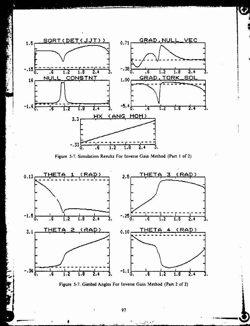
t,5__ 0.71__RAD" NULL__VEC

"'iS0, .6 i,2 i,B 2,4 3. "'3B0, ,6 t,2 t,8 2.4 3,

i.00 GRAD. TORK_SOL-5,4 ' ' '-t,6 _.

3.3 . ,_

"'330. ,6 i.Z t,8 2,4 3,

Figure 5-7. Simulation Results For Inverse Gain Method (Part ! of 2)

0.13 THETA, i ,(RA]::)) : 2.5

"

, _________-t,50 _ • I I I, .6 i,2 1,8 2,4

THETA 3 ,(:RAp)

I I I3, "'250. t6, 1.2 i,B 2,4

3,1 0,i0

I -i, I . i I

Figure 5-7. Gimbal Angles For Inverse Gain Method (Part 2 of 2)

5

9"/

0.29 THIDOT TORKI | ! !

I I I"3'30, ,6 t,2 1,8 2.4

t.5 TH2DOT TORKI I I I

",860,

TH3DOT TORI<I - I I I

I I I I,6 t,2 1,8 2,4

-.600.

t.9 TH4.DOT TORKI | I I

i I , I i -,230, I i I i,6 t,2 t,8 2,4 3, ,6 I,Z 1,8 2,4 3.

Figure 5-8. Torque Producing Gimbal Rates For Inverse Gain Method

(Rad,'Sec) (Part 1 of 2)

i P.

"=|

r2.,- '

4,6

-i,90,

THIDOT

I I,6 1,2

NULLI !

a

t i .t,80t.8 2.4 3. ,

6,9 TH3DOT NULLI I I I

I I I I.6 1,2 1,8 2,4 3,

6.5

-,99

TH2DOT NULL0,57 TH4-DOT NULL

I I I |

m

3, "6'30,

i

I I I I_ I I IO, .6 1.2 t.8 2,4 ,6 t.2 1,8 2,4 3,

Figure 5-8. Null Gimbal Rates For Inverse Gain Method (Rad,'Sec) (Part 2 of 2)

98

r /, i---r,--,---10, .6 _,_ _.,8 _,_ _.

0.97

Figure 5-9. Jacobian Minors For Inverse Gain Method

The measure m is seen to dip somewhat as the singularity is approached, but definitely

remains non-zero; Ha, is seen to continuously increase until the end of the simulation.

The reason for singularity avoidance may indeed be that this method does not con-

strain null motion to e.lways increase the singularity measure, 'hereby allowing the gim-

bal angle trajectory to depart from local m-extrema, as seen from the non-zero values

of the null projection encountered during the simulation. The effect of the torque and

null projections on the singularity measure is clearly seen in the corresponding plots;

for t < 0.6 sec. , the torque solution increases the system gain, whereas the null projec-

tion decreases it. This is clearly evident in the slight dip in the plot of singularity meas-

ure over this time period. It is also seen that the null projection is very small near the

singularity, and actually remains at zero near the end of the run (after about 2.4 sec.),

when m has reached its maximum. A physical interpretation of this maximum m, in

terms of the mechanical analog, suggests that the linkage may not be instantaneously

99

reconfigured by null motion to a iocally larger value of m; this determines the local

extrema of the singularity measure (in the absence of a torque request), hence yields a

zero gradient projection on the null-vector From the gimbal angle plots, it is seen that

gimbal #2 is e, entually rotated completely towards the the torque direction. Gi:nbal #4

also moves to compensate for the off-axis torque errors introduced by the motion of

gimbai #2 while it is being reconfigured from the "hung-up" negative projection orien-

tation.

In Figure 5-8, both the torque and non-torque producing gimbal rates are shown.

Large spikes are evident in both rates near the singularity. The largest magnitude of the

applied null motion occurs at these spikes, where the null-projection is very small, tht:s

rendering these motions ineffective i_, affecting the singularity measure. These large

null-rates are due to the correspondingly large value of the null constant and small (but

non-zero) valued minors that generate these motions. From the minor plots presented

in Figure 5-9, it is clearly seen that the singularity is avoided, since only minors =2 and

n4 approach zero near t = I. 15 sec. Due to the large gimbal rates, this method cannot

be considered a viable candidate for a Steering law.

Because of the substantial null motion projection onto the m-gradient seen in Fig-

ure 5-7, it is seen that the gimbal angle trajectory generated by this approach is not

locally m-extreme. In addition, as noted above, this method added most of the null

motion when the system was already nearly singular. In order to properly avoid the

,, singular state, it would have probably been desirable to add null motion earlier in the

7,_ tralecto_', when m > I and the system was far-removed from problematic orien-

i rations. A second form of the inverse gain was thus formulated to accomplish tl)is

I I00

strategy. The weighting factor is now chosen to also provide substantial null motion at

high-m configurations:

I 6

m /fm>l

2= _ 1 /fro< 16

m

(5-11)

Simulation results using this "second inverse gain method" are shown in Figures

5-10 through 5-12. The magnitude of the null-constant was limited to ,_._ = 3. From

Figure 5-10, it is seen that this method is able to avoid the singularity. Comparing

Figure 5-10 to Figure 5-7 , it is seen that the singularity measure has a larger magni-

tude throughout the simulation for this updated method, implying a wider margin of

singularity avoidance, hence smaller torque producing gimbal rates. The null projection

appears ve_ different for this method, which indicates that a different gimbal trajectory

was generated. This is evident by looking at the corresponding gimbal angle plots,

where it is obvious that gimbals #1 and #3 followed markedly different trajectories than

encountered in the previous test (Figure 5-7). Because the singularity was better

avoided, gimbal _2 is seen to have a much smoother trajecto_'.

Both the torque and non-torque producing gimbal rates are shown in Figure 5-1 !.

Comparing these plots with those in Figure 5-8, it is clearly evident that the gimbal

rates generated by the second form are much smaller than those from the first form.

Most importantly, no spikes are apparent in the gimbai rates calculated using the se.c-

ond method. Looking at the null rates, it is seen that they no longer peak at large val-

ues near the singularity. These rates are less than half as large as the corresponding

null rates calculated by the first form. From the minor plots presented in Figure 5-12.

!01

...... _.;,__-;___............ _ _.

O.71 • , -

"'690. ,6 t.2 i,B 2.4 3.

3,3 NULL CONSTNT 0,89 GRAD.TORK_SOL

HX (ANG NON)3.3 I ' I

-'330. .6 I_2 i.8 2.4 3.

Figure 5-10. Simulation Results For Second Inverse Gain Method (Part i of 2)

0,13 2.5THETA i (RAD)

' " I" "I ! I ' 'THETA :::3 ,(RAp)

o. ,_ i.2 t,8 2., _. o, ,_ i.2 1.8 2,4 3,

3.6 T I'T'IETA, 2 (RA,D) 0.40 ,,'r,HETA 4 < RAp) .

I I I I .. "I I I . I I.-'J'60. ' .6 1.2 1.8 2.4 3. '60. ,6 t.2 i.e 2.4, 3.

Figure 5-10. Gimbal Angles For Second Inverse Gain Method (Part 2 of 2)

m _ ....

102

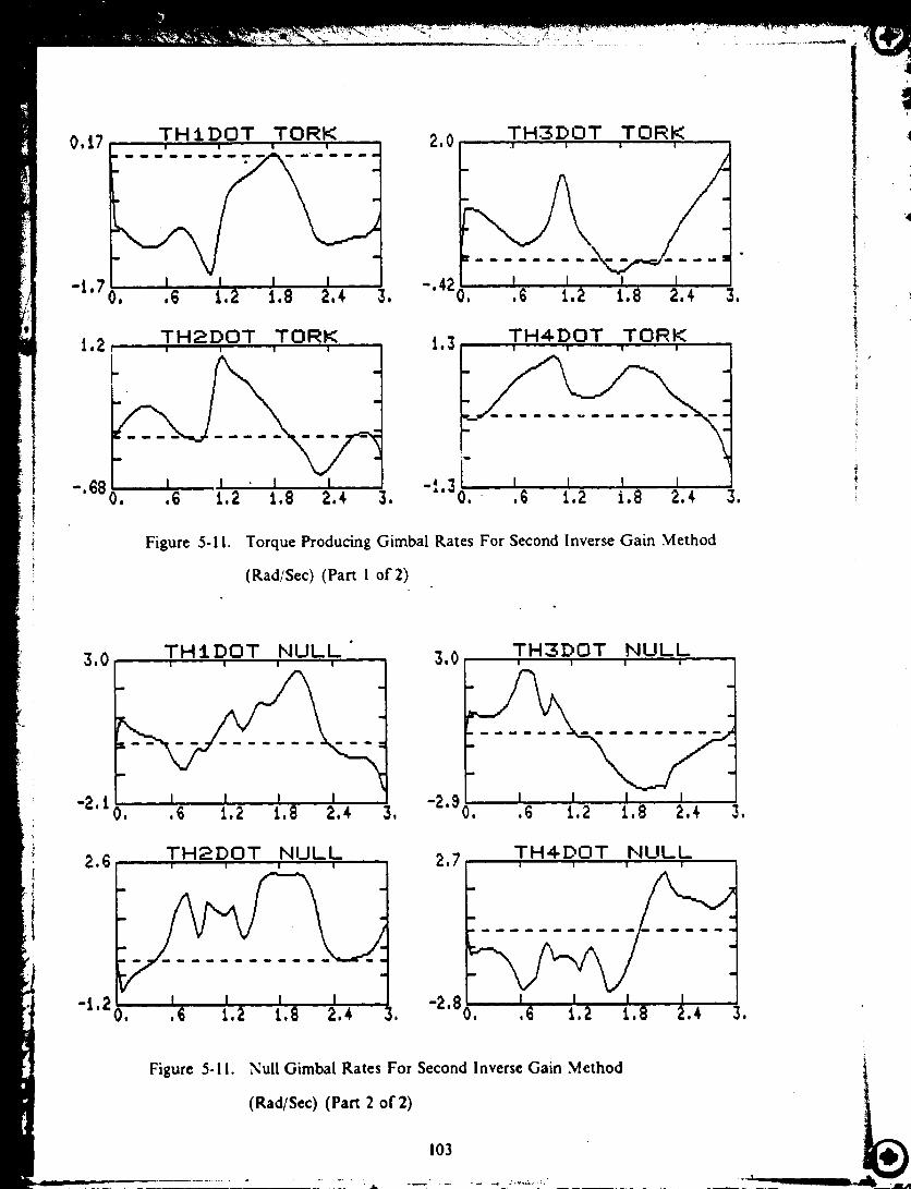
0,i7

-i,7

-,68

THiDOT TORK

I I I IO, ,6 t,2 1,8 Z,¢ 3,

i.2, TH2DOT TORK ,I I I |

I L • I I ,,O. ,6 1,2 1,8 2.4, 3.

2,0 TH3DOT TORK

-,420 ' 16 I I Ii.Z i.8 2.,t 3,

i.3TH4DOT TORK

I I I i"t'30..16 i.2 i.8 2.¢ 3,

i

Figure 5-11. Torque Producing Gimbal Rates For Second Inverse Gain Method

(Rad/Sec) (Part 1 of 2)

3.0 THtDOT NULL "!

-z, iL j .,. .m. j.v, ._ z.= z._ ,.., 3.

2,6TH2DOT ,NULL., ".

-i,2 I I I iO, ,6 1.2 1.8 2.4 :

3,0 TH3£)OT NULLI I I I

,6 i,2 1,8 2.4 3,

2,7TH4.DOT NULL

I I I I

-

1 I I"2'80. 16, i.2 i.8 2,¢

Figure 5-11. Null Gimbal Rates For Second Inverse Gain Method

(Rad/Sec) (Part 2 of 2)

103

III I I

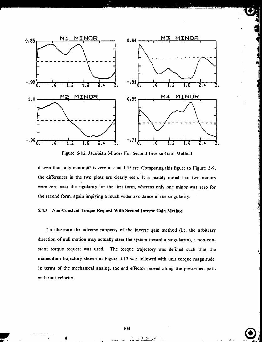
0._5

-.99

1.0

-.9_

M1 MINORi

I I I I

r__ mmo ]

I I I IO, ,6 1,2 1.G 2,4 3.

0,64

",gtO,

P13 MINOR

• I | I I i

I I , ,I I,6 1,2 1,8 2,4 3,

M2 MINORI I I , ,i I

O. .6 1,2 1,8 2.4 3.

0.99

-.710,

M4 MINOR

-I I I I.6 1.2 1,8 2,4 3,

Figure 5-12. Jacobian Minors For Second Inverse Gain Method

it seen that only minor #2 is zero at t = !.15 sec. Comparing this figure to Figure .5-9,

the differences in the two plots are clearly seen. It is readily noted that two minors

were zero near the sigularity for the first form, whereas only one minor was zero for

the second form, again implying a much wider avoidance of the singularity.

5.4.3 Non-Constant Torque Request With Second Inverse Gain Method

To illustrate the adverse property of the inverse gain method (i.e. the arbitrary

direction of null motion may actually steer the system toward a singularity), a non-con-

stant torque request was used. The torque trajectory was defined such that the

momentum trajectory shown in Figure 5-13 was followed with unit torque magnitude.

!n terms of the mechanical analog, the end effector moved along the prescribed path

with unit velocity.

!04

Hy

1.18

0.59 ___

0.59

ner:

Figure 5-13. Momentum Trajectory For Non-Constant Torque Simulation

To simulate this maneuver, the torque request was defined in the following man-

0.7071 ]z_ = 0.7071 for t < 0.83 sec.

0

[o,o 1z = 0.7071 for 0.83 sec. < t < 1.626 sec.0

Simulation results for this maneuver are shown in Figures 5-14 through 5-16. The

magnitude of the null-constant was limited to 3. From Figure 5-14, it is clearly seen

that the system becomes singular just before the torque direction is switched (at t =

0.83 sec.). From this figure, it is observed that the null projection remained negative

until the switch time was reached, thus the effect of adding null motion was to reduce

the singularity measure. From the torque projection plot, we see that torque produc-

105

i I I1_

ing gimbal motion does not contribute appreciably to the singularity measure. A large

spike at the switch time is also observed in the torque projection plot, indicating a loss.

of control along the commanded torque direction. The reduction in m now is almost

entirely due to the addition of of null motion.

Gimbal angles are given in Figure 5-14, and both torque and non-torque produc-

ing gimbal rates are shown in Figure 5-15. Large ._pikes are evident in the torque pro-

ducing rates at the switch time, as would be expected, since the system is nearly

singular in the direction commanded after the switch. From the null motion plots, it is

seen that the magnitude of the null motion is zero at the switch point, since all Jacobi-

an minors are singular. This is clearly seen in Figure 5-16.

5.5 CONCLUSION

We have shown that the inverse gain method is able to avoid the Elliptic singulari-

ty. It has also been shown that the performance results of the second lbrm of this

method (which applies substantial null motion at high rn states) are superior to the first

form (which applies most null motion when the magnitude of m drops significantly_.

The calculated null-rates, however, are still high for the second form. This feature,

when combined with the property that the non-directional applied null motion may

actually steer the system to a singularity (as was demonstrated in the non-constant

requested torque simulation), make this approach inappropriate for application as a

generic Steering law.

106

®

1.6 SQRT(DET(J.IT) ) 3.3 NULL CO_ i

-'160. .36 .72 1.08 1.44 1.8 36- - "T- - - r - - -_- -

0.64 HX (ANG MOM) 0,81

-,06 ,. ,36 ,72 i.08 1,44 ,8 -l'01

HY (ANG NOM)

-,i30. .36 .72 i.08 1,44 1.8

GRAD ,. N UL,L_ V E C

), ,3_ ,72 1.08 i,44 ,8

i5 GRAD. TORK_SOL

-2'20, ,36 ,72 t.08 t,44 ,8

Figure 5-14. Non-Constant Torque Results For Second Inverse Gain

Method (Part 1 of 2)

0,27 T,HETA 1 (RA,D) 3, t T,HETA 3 ,(RAp)

-,31-'3°0, ,3_ ,72 i,oBI,,_4 o. ,3_ ,7_ 1,08i,44 ,a

0.76 T ,HETA, 2 ,(RA,D ) ,.,n..4n. THETA, , 4 ,(RAD, )

...?:z._.?

w' _ -,9_ -t.t

_._ o, ,3G .72 t,08t,_4 o. ,3_ ,72 t,08t,4,,t,8

mR' Figure 5-14. Gimbal Angles For Non-Constant Torque Request (Part 2 of 2)

D_ 107

3

1,4 7,3 .,. ;H,.,,,,; .THIDOT TORK

-' o, t,4+ ,s-,73,.- i,08 .36 ,72 1,08 i.44 1,8

/ 1.3 1,3.__ TH4DOT TORKI '= i, I' ' l _ I

./?

r

r

-. 9t O, 136'

TH2DOT TORK'= • " " 1 " =' I !

I I, I.72 i,08 i.44

Figure 5-15,

J, i,

-7.40. , _ I .ii.8 ,36 .72 i.O8 I.44

Torque Producing Oimbal Rates For Non-Constant Torque Request

.8

(Rad/Sec) (Part 1 of 2)

t.7 THIDOT NULLI I I I

t I I, ,I,36 ,72 1.08 i.44 1.8

3.4 TH2DOT NULLI ; I " | • '

i

I I I I .,,36 .72 i.08 1,44 1,8

2,8

-,31

TH3DOT NULL' =' I I " • I "

p

O, ,36 ,72 1,08 t,44.

0.30

-I,60,

TH4DOT NULL' ! _ 'I I = ' ' I ' '

i ,. ,I ,, I I,36 .72 t,08 1.44,

t.8

,8

Figure 5-15. Null Gimbal Rates For Non-Constant Torque Request

(Rad/Sec) (Part 2 of 2)

108

......... ..._..n_ S....

/ IJ -1.2

M3 bIINOR

. ' . . ]

I

I I I I. .36 .72 t.08 t. 44 l,B

. M4 M I,NOR

, ,36 ,72 i.08 1,44 1.8

Figure 5-16. Jacobian Minors For Non-Constant Torque Request

1

109

CHAPTER 6

REDUNDANCY RESOLUTION VIA THE SINGULARITY ROBUST

INVERSE (SR-INVERSE)

6.1 INTRODUCTION TO THE SR-INVERSE

The results of Chapter 5 indicated that real-time avoidance of internal Elliptic type

singularities cannot be adequately accomplished using any of the available Steering

laws or any of the proposed methods. It was seen 'hat the torque solution produced by

the Moore-Penrose pseudoinverse eventually drives or restricts the system to a singular

configuration. Since solving the torque equation exactly was demonstrated to drive the

system directly to a singularity, one might surmize that if small torque errors are

allowed, it may become possible to avoid these types of singularities. lhi._ strateg',

presumes that the Outer controller (see Chapter 3) is structared to accomodate errors

in requested torque during attitude maneuvers. These errors can be considered to be

disturbance torques, and compensated through appropriate feedback.

One method of accomplishing this is provided by the Singularity Robust inverse

(SR-inverseL proposed for manipulators in [21] as an alternatiw to me .Moore-Penrose

pseudoinverse. [,sing this method, an approximate output torque close to the desired

torque can be generated, even when the Jacob[an matrix is singular. Accuracy of solv-

ing the torque equation is traded with feasibdity of the solution (_.e. gimbal rates

remain tin[re and bounded in exchange for the build up of torque error near asmgular

configuration).

[hc SR-inverse is obtained by solving the Following minimization problem:

II0 ®

| ermn y_rW e

where e_.=

IV=

T-s0]0 ,;

I)"1 [ 0 ]E o ] w-, _,

Setting ll', equal to the identity' matrix, (ll"_ = !). and W: = _c/, the SR-inverse is

obtained:

j= = jr(j jr + _;i)--1 (6-1)

"l-he particular solution can be written in terms of the SR-inver'se as:

_e = jr(j jr + ei l )-Ir 16-2)

6.2 PROPERTIES OF SR-INVERSE

The particular solution obtained using this method is still orthogonal to the homo-

gcncous solution. This is easily shown by evaluating the inner produ:'t of the two sol-

utions:

< Op.O/t > = O_T.o_H = ).( J Jr + gi)-I j_,_. = 11

The above relation holds, since J __'= 0 by definition of the null-vector. The robust-

,_ ness property of this method generates feasible solutions to the torque equation even at

Ill

_ .

or in the neighborhood of singular points. At singular points, the pseudoinverse

becomes singular, (i.e. results in infinite rate solution), whereas the SR-inverse still

returns a finite rate solution. It is seen that the pseudolnverse is identical to the SR-in-

verse with K = 0. The scalar weighting factor K expresses the tradeoff between exact-

ness and feasibility of solution. For small values of _, a small error is introctuced in the

torque solution. Small values of _ also yield large rate magnitudes in the neighborhood

of singular states. As K grows, however, the torque error calculated near a singular

state increases and the calculated gimbal rates decline.

The SR-inverse approach, however, is not without shortcomings. The most crucial

problem is that if"the system does become singular using this method, and a torque is

requested along the singular direction, the SR-inverse is unable to generate non-zero

torque producing gimbai rates. The system could then be trapped in the singular state.

This property is shown by the Singular Value l)ecomomposition of the SR-inverse.

which for the 4-CMG system is:

y_ = I'£=L 'r (6-2)

where .,x'_ =

a_ 0 0

2 a2 0at + K

0"30 o_+K2

0 0 a3 + _(

0 0 0

U = Matrix (3 x 3) of left singular vectors [ span ratzge space ofJ )

V = 3latrix [4 × 4) of right singular vectors ( span domain space ,J'J )

[;sing (6-3), the particular solution (6-2) can be written as:

112

®

_.p = V_':uT T_ (6-4)

If the torque request _Tlies along one of the column vectors of U, the gimbal rates

computed by the SR-inverse are given by:

_k

O" i{6-5)

up = 2 _v_cr: +K

From (6-5), it is seen that if one of the singular values, a,, is zero (i.e. system is singu-

lar) and the torque request is along the left singular vector, _t_u,, corresponding to this

singular value, the output becomes zero. In this case, the gimbals will not move, thus

trapping the system in the singular conliguration. Unless this singularity allows escape

by null motion (as discussed in Chapter 4), there is no possibility of removing the sys-

tem from the singular configuration.

6.3 DETERMINATION OF WEIGHTING FXCTOR

To overcome the problem of conflicting requirements on the value of the weighting

factor, it is made to vary with the nearness to singularities. In this way, K will have a

large value near singularities, an,t small or /ero value away from singularities, lhe

weighting factor is thus chosen in the following manner:

113

, t

[,

xZ

I

//q

P

IF m > mcR

K=O

ELSE

IF K°_<

KOK --

ELSE

K -_- Kma x

THEN

Kmax THEN

where mcR = Critical :alue of m

Ko = Constant

Kmax = Maximum value of weighting factor

In this fashion, the weighting factor is adjusted according to distance from singularity

by inversely scaling with the singularity measure. The reason for the applied maximum

value is to prevent the determinant of the square Jacobian matrix (J Jr + _/) from

becoming too large; in this case, the torque producing rates would correspondingly

grow ve_' small, which would require an extended period of time for the gimbai angles

to change. Bv imposing an upper limit, the response of the system is essentially speed-

ed-up.

6.4 SINGULARITY AVOIDANCE PROPERTIES OF SR-INVERSE

i

In order to examine the singularity avoidance properties of the SR-inverse, simu-

lations similar to those in Chapter 5 have been carried out. The SR-inverse is com-

puted numerically, using the symbolic inverse of the square Jacobian matrix. Results

from tour different simulations are presented in this section; these are:

114

a) SR-Inverse

b) SR-lnverse With First Gradient Method

c) SR-lnverse With Second Gradient Method

d) SR-lnverse With Second inverse Gain Method

All simulations used the same parameters as given in Chpater 5. The critical value of

the singularity measure was chosen as mcR = 1.0, with constant N0 = 0.1. The plot-

ted percent torque error is determined from the dflFerence between requested input and

CMG output torque, i.e.:

% Torque Error = 100(__ - JO e)

where _Oeis determined from (6-2).

6.4.l SR-inverse

The results of this simulation are shown in Figure 6-2. The maximum allowed

value of the weighting constant was Km_, = 0.2. The plots clearly show that the Ellip-

tic singularity is not avoided, it is evident that even though m--* O, the determinant of

the square Jacobian matrix (SQJ DET) remains nonzero. This illustrates a fundamen-

tal property of the SR-inverse; gimbal rates can still be computed when the Jacobian

matrix is singular. [he value of_( (SR INV GAIN) is noted to increase as the singu-

larity is approached in order to allow the square Jacobian matrix to be inverted (see

(6-2)). From the gimbai angle plots, it is seen that gimbals _2 and #4 remain station-

ary, as was also the case for the Moore-Penrose pseudoinverse method. This result

indicates that the SR-inverse similarly cannot avoid Elliptic type singularities without

115

. ii.,--,_,.,_ _ --

assistance, essentially because the primary difference between the SR and the M-P

inverse is in the magnitude of the particular solution. The "direction" is still the same

(i.e. orthogonal to null-space), as illustrated in Figure 6-1, for a one-dimensional row

and null space.

61q

$R-II_VERSE

_. = jr( j jr + _l)-'x

ERROR

MOORE-PENROSE P5 EUDOIb/VERSEI _"i_' _, = J_ J i _)-'

I II II I

.:,

I I

Figure 6-1. Solution Space Visualization

The complete torque equation solution is spanned by the row and null space. The

SR-inverse as well as the M-P inverse solutions lie in the row space. From Figure 6-1,

it is seen that the only difference between the two is the length (or magnitude) of the

torque producing gimbal rates. Because the SR-inverse tends to produce smaller gimbal

rates near singular regions, it allows more time for the application of null motion, thus

introduction of null motion may prove more effective, as will be demonstrated below.

Since the primary effect of the SR-inverse is along the direction of commanded torque,

116

the SR-inverse applied without null motion is indeed expected to have analogous singu-

larity avoidance properties to the M'-P inverse, as was demonstrated in Figure 6-2.

6.4.2 SR-Inverse With First Gradient Method

:

The simulation results for this method are shown in Figure 6-3. The weighting

constant was limited at K_, = 0.2 . From Figure 6-3, it is seen that the singularity is

again not avoided. The reason for this is the same as that given in Chapter 5 for the

M-P inverse with this gradient method; essentially no null motion was added because

the gimbal angle trajectory, remained at a local m-extremum. From Figure 6-?, it is seen

that gimbals _2 and #4 do not move, allowing the system to become singular at

tlx = !.15.

6.4.3 SR-Inverse With Second Gradient Method

Simulation results for this approach are shown in Figures 6-4 through 6-6 . The

weighting factor was limited at K_ = 5, although this limit was not neccessar 5' in this

case, since K remained under 0.28, as can be seen from Figure 6-4. Since the singularity

measure remains well above zero in this test, the singularity has been avoided. From

the momentum component plots (I!X, ttY, tIZ), it is seen that the momentum trajec-

to_' is diverted about the singularity, causing about 70% torque error in the .g-direc-

tion, and considerably smaller errors about the Y and Z axes. The effect of null motion

was to alter the Jacobian matrix, thus enabling the SR-inverse to generate finite off-

axis torque errors that aided in skirting the singularity. Singularity avoidance is accom-

plished by not forcing the system to go directly through the singular momentum state.

117

1,2 DSQ, RT(,det,(JJT) )

i , I I I I , ."'t20, ,6 t,2 t,B 2,4 3,

t.6 SQJ DETI I i !

I-'*_o'.'-;',__.2 _._ 2,, 3.

i.3 HX (ANG• I I I

MOM )

i30 .... j i I"' J..6 i 2 i.8 2.4 3e i i

Figure 6-2. Simulation Results For SR-lnverse (Part 1 of 2)

0.16 THETA i (RAD) i,7 THETA 3 ,(RAD)

m

"1'70, ,6 i,2 t,8 2,4 3, "'170, '16 i l lt,2 i,B 2,4 3,

0,37 THETA .2 <.R.A.D ) .... i4 T HETA 4. ,(RAp)

1( I _

"3'8o.I_ t.2 t.8 a., 3. -t.%. :i- , .,6 t,2 i,8 2.4

Figure 6-2. Gimbal Angles For SR-Inverse (Part 2 of 2)

118

1

®

-.t6 ),SR--INV

0,22 , ,

f /-.02 I

0, ,6 1,2

I0

t2NULL CONSTNT

I I

t,8 2,4. 3, -1'20, ,6 t,2. t,8 2,4 3,

Figure 6-3. Simulation Results For SR-Inverse With First Gradient

Method (Part 1 of 2)

O,t_

-1.

THETA i (RAD) 1,7I ! I t

I I , I IO. ,6 1,2 1,8 Z.4

THETA 3 ,(RAp)

THETA 2 (RAD) (RTHETA 4 AD)

"7'50. ,G i,2 i.8 2.4 3. "3'30. ,6 1,2 1,8 2,4 3.

Figure 6-3. Gimbal Angles For SR-lnverse With First Gradient Method (Part 2

of 2)

119

A complimentaryreasonfor the avoidanceisclearif wecomparethe X-momentum

plots of this approach with those of the inverse gain method in Chapter 5

(Figure 5-10), where one can see that the SR-inverse solution lags the inverse gain sol-

ution. At t = 3 see., the difference in momentum between the two methods is approxi-

mately 0.6 units. This illustrates the explanation given earlier; i.e. the response is

slowed down sufficiently to allow more time for null motion to act. Given enough time

for reconfiguration by null motion at each simulation interval, the singularity measure

could approach its global maximum. In this way, the gimbal angles are free to follow a

globally maximum singularity measure trajectory, as opposed to a locally maximum

trajectory that is generated by gradient methods. Following a globally maximum trajec-

tory provides a superior means of accomplishing singularity avoidance.

From Figure 6-5, it is seen that both gimbals #2 and #4 are moved in this case,o

allowing gimbai #2 to be "unlocked" from its anti-parallel orientation. From the minor

plots, it is seen that only one minor (M2) becomes -.ingular at t = 1.15 sec. Looking at

Figure 6-6, it is seen that both torque and non-torque producing rates have reasonable

magnitudes (not exceeding i.8 rad,'sec); by avoiding the singularity, the requirement for

small gimbal rates is implicitly met.

6.4.4 SR-lnverse With Second Inverse Gain Method

Simulation results for this method are shown in Figures 6-7 through 6-9. The null-

constant ( NULL CONSTANT ) was limited to Am,, = 3, in order to limit the magni-

tude of null-gimbal rates. The maximum allowed SR weighting factor was K,_ = i.

Enforcing this maximum value was again not necessary in this case, as can be seen

from the SR-inverse gain plot in Figure 6-7. The singularity measure plot, also on this

p,

120

®

,DSQRT (,det,( JJT ) )

"'I_0, - i_ 1.2 I;8 2.1 3.

/./

j.

i!c

#_I0 i i m , .

-.2o:---,_._-_.2....._.827;-ISR--INV GAIN

0'281 '_ ". J J l

-,03 ,6 1,2 t.8

i

t2,4 3,

0.76 NULL CON,STN T

6,6_

" 0. .6 i.2 i,8 2.4 3.

0,14 GLRAD NULL_VECi l Ill i i

-,50 , I,.' ._ 1.2 {:8 _._ :,

0,98 GRAD. TOR,K_SOL

"t'70, ,6 i.2 1.8 2,4 3.

Figure 6-4. Simulation Results For SR-Inverse With Second Gradient

Method (Part 1 of 2)

m_

IIO'

_.272'7_' ANG NON)

0. ,6 i,2 1.8 2,4 3,

77 HY (ANG NON)i ii i.i • i i i i i ii i

m

I -0 -

-8,2 ).

0 03

' i

/ 1'_' _.2." 1:8 _.4

t, ii

HZ (ANG hlOM)i

I

.6

-_' "" ;" ' ""' " 1

• I I J

1,2 i.8 2.4 3,

74 Y., TOR, I<I ,ERR,OR

-7,4 2. i,8 2.4 3,

1.2. 7. TORK2 ERRORi i g • ,, i ! i ,¶

_ ! I I ._-t0 ). .6 1.2. 1.8 .4. ,.

36 1 7. TORK3_,E.RROR t

3.7& t_ ' ' "'i,2. 1,8 2,4 3,

Figure 6-4. Momentum Trajectory And Torque Errors For SR.-lnverse With

Second Gradient Method (Part 2 of 2)

121

0,21

, T,HETA, 2 ,(RA,D,)

I I I I,0. ,6 i.2 l.B 2.4

"'140a

0.77

3, "'080',

T,HETA 4 (RAp)

I I I I,6 1.2 1.8 2,4 3,

Figure 6-5. Gimbal Angles For SR-Inverse With Second Gradient Method (Part

1 of 2)

0,90-- Mi MINOR

-.09 r I i j0. ,6 1,2 1,8 2.4

1.0 M2 MINOR! i I I

-,14

5|

0,61 M3 MINORl I I !

-.570, i i _ l,6 1,2 1.8 2,4 1

I I, I I). ,6 t.2 i.8 ;!.4 3,

Figure 6-5.

0.68, , M4, MI,NOR,

.91" ' 8 2.4

Jacobian Minors For SR-lnverse With Second Gradient

_0

Method (Part 2 of 2)

122

®

0.37

Q _

TH1DOT TORKI ! I !

-1,20, t t t t,6 t.2 1.8 2,4 3,

0,i3_

f-t,t

O,

1,2 TH3DOT TORK

0_ - --[" I I-,t2 6 11,2 1,8 2,4

TH2DOT TORKI I ! !

I I I I,6 i,2 t,8 2.4 3,

0.06

m

m

3,

TH4-DOT TORK

- 620 I I I t' , ,6 i,2 t,8 2.4

Figure 6-6. "lorque Producing Rates For SR-Inverse With Second Gradient

Method (Rad/Sec) (Part 1 of 2)

|

I

1

i:

O.42 THiDOT NULLI I l I

I I I I0, ,6 i,2 1,8 2,4 3,

0,25 TH3DOT NULLI I I i

.....

-,66! 1.8 2.4 3.

0,2i TH2DOT ,NULL

"=;'- _'" _

I I I I-1.70, ,6 1,2 t,8 2,4 3,

Figure 6-6. Null Rates For SR-lnverse With Second Gradient Method

(Rad'Sec) (Part 2 of 2)

123

page, indicates that the singularity is again avoided. The maximum torque error intro-

duced via the SR-inverse is approximately 25% in the X-direction, when the system is

near the singularity. Comparing results obtained in Chapter 5 with the second inverse

gain method using the M-P inverse (Figure 5-I0), it is observed that both the null-con-

stant and torque solution projection are smaller for the SR-inverse approach. Because

of the torque errors introduced by the SR-inverse in the singular regiov., however, a lag

of 0.2 units is evident in the X-momentum plot for the SR-inverse. The gimbal angles

and minors are shown in l:igure 6-8. Near the singular momentum state t

ttx = 1.15, t _ 1.15 see.), it is seen that none ofthe minors are singular, ie. are zero,

Comparing the gimbal rates from this approach, shown in Figure 6-9. to those

analogously obtained from the M-P inverse, the peak torque producing gimbal rates

calculated by the SR method are seen to be approximately 0.4 rad scc smaller, l'hc null

rates, however, are essentially the same.

6.5 NON CONSTANT TORQUE REQUEST SIMULATION

In this simulation, the same non-constant torque request used in Chapter 5 lbr the

M-P inverse with the second inverse gain method is applied to the SR-invcrse equipped

with the same null algorithm. Simulation results are shown in Figures 6,-111 through

6-12 . The maximum allowed SR weighting factor was K_, = 0.2, while the maximum

value of the null-constant was 2m,_ = 3. From Figure 6-10, it is seen that the system

is driven to a singular state, even though the SR-inverse is used. It is also obscrved

that at the singularity any null motion is inellective since the null projection there is

zero. "lhe reason tot this is that the null vector is identically zero at this singularity.

124

®

i.G DSORT (clef (JJT))

"' 0. ,6 1.2 1.8 2.4 _.

Figure 6-7.

NULL CONSTNT

0, ,6 i,2 I,B 2.4 _,

0.68 GRAD.NULL_VEC• , i , i i

I I m-,72 _, .6 1.2 1,8 2.4 i.

GRAD.TORK_SOL

0.85

Simulation Results For SR With Second Inverse Gain Method (Part

I of 2)

M

a

?

0,20

I0,4

-2.2

1

7.

2.Sl I _ ," _.'6

5,7 X. TOR..K2 ERROR

-.e8_, ,._ ,1.2 _.8 _._7. TORK3 ERROR

2.7 I ....

",6 1.2 t,8 2,4

TORKI ERROR _

3.

I

Figure 6-7. Momentum Trajectory And Torque Error For SR With Second

I'i

Inverse Gain Method (Part 2 of 2)

125

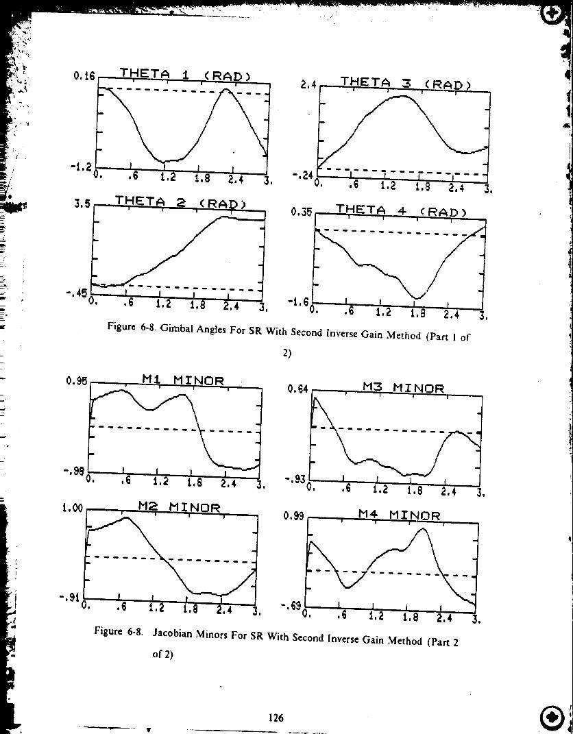
0,16 2,4

, . ,

0.35

Figure 6-8.GirnbalAngles For SR With Second InverseGain Method (Part I of

2)

i.O0 M2 MINORI I ' I I I

-'9t0. .6 t,2 1,8 2.4 3.

0.99 I"l4. MINOR= I • i, I i I ' I

I I I I ,,6 1.2 1.@ Z,4

Figure 6-8. Jacobian Minors For SR With Second Inverse Gain Method (Pan 2

of2)

i

126

O,17 TH:1.DOT TORK| ! I I

I I I I ;.6 1,2 1.8 2.4 3,

t,3

"'350, 3,

THT])OT TORK

I I I Y,6 1.2 1,8 2,4

0.80

-,72

TH2DOT TORK t,t TH41)OT TORK

I I I I - 480, I I 1 I0. .6 i,2 t,8 2.4 3. ' .6 1.2 1.8 2,4 3.

Figure 6-9. Torque Producing Gimbal Rates For SR With Second Inverse Gain

Method (Rad/Sec) (Part 1 of 2)

2,9

-1,30,

THIDOT NULL

I I I I,6 t,2 t.8 2.4 3,

3.0 TH3DOT" NULLI I I I

-2,7 l t I I0, .6 1,2 1,8 2.4 3,

2,7

-i.20.

TH2DQT NULLI I I l

,6 i,2 t.8 2.4 3.

2,5TH_DOT NULL

80 ' I i-2. t6, t.2 i .8 2 ,4 |

Figure 6-9. Null Gimbal Rates For SR With Second Inverse Gain Method

(Rad/Sec) (Part 2 of 2)

127

since all Jacobian minors are zero (see Figure 6-11). The momentum trajectory and

torque errors are shown in Figure 6-10, from which it is seen that substantial torque

errors are generated by the SR approach. Comparing Figures 6-10 and 5-14, we

observe that the system remains singular for a longer period using the SR method,

whereas the torque projection spike in Figure 5-14 is at least an order magnitude larger

than the corresponding spike for the SR method, creating proportionally larger torque

producing gimbal rates. The difference in momentum trajectory followed by both meth-

ods is clearly evident from this comparison.

From Figure 6-11, we observe that all minors are simultaneously zero for a sub-

stantial period of time. Comparing the minor plots in this figure to those in

Figure 5-16, it is seen that the minor trajectories for both methods are essentially the

same up to the switch time (0.83 see.), and very different afterwards. A similar effect is

seen when comparing gimbal angle trajectories in Figures 6-11, 5-14.

The superior performance of the SR approach is evident from the results in

Figure 6-12. From this figure, it is seen that the peak torque producing gimbal rates do

not exceed i.4 tad'see, as compared to 7.4 rad sec for the M-P based method in

Figure 5-15. In addition, the SR-inverse is not seen to generate large spikes in gimbal

rates that were noted in the M.P results, l'he null-rates for the SR method are signif-

it antly smaller, as also seen in these plots. This is due to the different gimbal angle tra-

jectory that the M-P method followed alter the switch time, which resulted in a higher

singularity measure state, as well as higher values for the minors, in conclusion, the

superior performance of the SR based method over the corresponding M-P based

approach is clearly evident from this simulation. As discussed before, however, if the

128

®

requestedor uc irecionatheswichimew saongthesi.ad--oncor,e' i:_,: sponding to the singular momentum state, the SR approach would not have been able _

_f_ " ',! to extract the system from the singular configuration, since zero torque producing rates

_i I are generated.

6.6 CONCLUSION

It has been shown that the SR-inverse is able to avoid the Elliptic singularity at

llx = 1.15 only when equipped with an appropriate null motion algorithm. ]'he supe-

rior performance of this method has also been shown for a case requiring a non-con-

stant torque. The general singularity avoidance property of tile SR-inverse has tllso

been discussed, and it has been shown that the prime mechanism b_ which this method

avoids singularities is by slowing tile system response to an input torque request in the

neighborhood of a singularity, allowing more time for null motion to be applied. In

terms of the mechanical analog, the end-eflbctor velocity is reduced before reaching tile

singularity, allowing a longer interval over which null motion can bc performed. The

SR-inverse can also introduce linite torque errors orthogonal to tile requested torque

direction; although these errors aid in skirting the singular region, the slow-down along

the commanded axis, coupled with null motion, provides the most significant efl'ect.

129

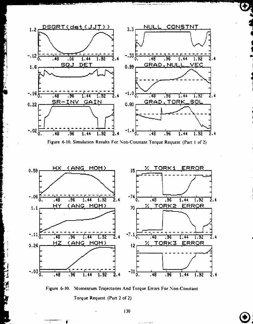
I,.2 DSQRT (,de+. (JJT) ) 3.3 NULL CON.STNT, /_....-,33 ?_ -,--lao.,48,_ i,.i,ga2,_ i..1,922,4

t,6 , SQ, J D,ET , , 0,99 GRAD',NUL,L--VEC

- -'_'''"-'" -i,0 , J L , ,

0.22, ,SR-I, NV GAIN 0.80 GRAD, TOR,K_SOL

-.02r'--,---i---r--_-t , ,48 ,96 1.44 i,92 2.4O, ,48 ,96 t,44 i.92 2,4 _i.4q_

Figure 6-10. Simulation Results For Non-Constant Torque Request (Part i of 2)

HX (ANG NON)0.59 ....

O, .4,8 .96 t.44 1.92 2,4

t,1 HY (ANG MOM)

.,i1_. 4

0.26 HZ (ANG HOP1)

O, .4,8 ,96 1.44 1.92 2, 4,

Y. TORK1 ERROR15 ....

-74 '.96 1.4'1' i.92 2,4'

7OD

m

m

:j--_71 _11-I ii

12 7.

I-3t

O,

TORK2

I I,48 .96

TORK3

I I

ERROR!

i A ,

1.4_ i.92

ERROR

,4

,48 .96 1,44 1.92 2,4

Figure 6-10. Momentum Trajectories And Torque Errors For Non-Constant

Torque Request (Part 2 of 2)

130

®

( RAD 0.870.50 "rHETA i ,> THETA 3 (RAD)• ! ! ' , | ! '

a

-05 " t " I I . J -7_ -.21 i i i . J, , ' 0. .48 .,6 i.44 1.92 2.4 0. .,B .96 i.44 i.92 2.4

[iLn _ THETA 2 (RAD) 4 a THETA 4- (RAD)VI a_ i l 11 1 II i I I i i I I I Ill i I II a I ] I I i l' I I ' i

I

"l'B0. .43 .96 1.44 I._2 2? -.41). .4B . 6 1.4 i, 2.4

I Figure 6-11. Gimbal Angles For Non-Constant Torque Request (P_.rt l of 2)

0.65 MINOR 0.B3I l

Mi,, ,i

I I

I .... I I I , -. 09 O_-,380, ,4.8 ,96 1.¢4 1,92 2,4

M3 MINOR

I , I I _ , 1,.4B ._6 t.4¢ t._2 2.4

I

w

,,,a.,, •

2,,.¸

M2

0.63

-.52 1 I

0. .48

M4. M I NORMINOR 0.62 ,......I l I | I I I

---.070 J ,, ,444.96 i 1.92 48 .9_ 1.44 t.92

Figure 6-1 I. Jacobian Minors For Non-Constant Torque Request (Part 2 of"2)

131

2,4

0.i$

-.85

THIDOT TORK| I ! I

D _ _ m m _ _ im, o u _ m m

mm , ,

I I l I0. .48 ,96 i,44 1.92- !.4

0,72 TH3DOT ,TOR,K

-,70 F I l I i l0, ;48 ,@6 t.,$4 i.92 2,4

0.42 TH2DOT TORK 1,4 TH4D, OT TOR,K

• "i"ii,'-i--!0-.--.7t J _ i2 ., "'" _48 .', i.92 _.,

Figure 6-12. Torque Producing Gimbal Rates For Non-Constant Torque Request

(gad/Sec) (Part I of 2)

, "411

1.5 i,_ TH3DOT,NULL, , , ,

-i.30 ' i . f i i-. 16 2. ,$ .48 .96 i. 4_, i. 92

0, i9

THIDOT NULLI I I

I l I I0, .48 ,96 I,44 1.92

TH2DOT NULLI mb I I I

I , I I I,48 ,96 i,44 t,_2-:,.o0.

m

I2.4

Figure 6-12. Null Gimbal Rates For Non-Constant Torque Request

(gad/See) (Part 2 of 2)

132 ®

W

CHAPTER .7

CONCLUSIONS AND RECOMMENDATIONS

In this thesis, the problem of spacecraft attitude control using redundant single

gimbal CMGs has been investigated. Specifically, the singularity problems associated

with a 4-CMG system has been examined, in addition to the formulation of a general

torque based Steering law for redundancy resolution. A Steering law using the S R-in-

verse with appropriate null motion has been shown to provide a promising approach to

singularity avoidance; by not restricting the system to produce the exact torque

request, singular CMG configurations are avoided.

t:

++

In Chapter 2, single gimbal CMG fundamentals were reviewed, and the mechanical

analog to the CMG system, the robotic manipulator, was proposed. It was shown that

both systems possess similar difficulties with singular configurations, and that results

from one area may be applicable to the other. A simple method of generating an

orthogonal null-space basis to the Jacobian matrix was also presentcd.

in Chapter 3, the control architecture for spacecraft equipped with single gimbal

CMGs was reviewed. A dual-level control structure using an Outer and Inner Control

loop was discussed, as wcll as the desirability of the Outer control loop to accomodate

occasional errors in torque delivered by the CMG system.

In Chapter 4. the singular states of single gimbal CMGs were classified, and a test

for null motion near a singularity was presented. Examples of the different types of sin-

gularities were presented for both the CMG system and a planar manipulator. The

singularity measure and its relationship to the null-space of the Jacobian was exam-

133

+

+

J

ined. It was shown that the magnitude of the non-singular Jacobian null-space vector

is identical to the singularity measure.

In Chapter 5, various torque-input Steering laws were reviewed, and alternative

singularity avoidance methods based on the Moore-Penrose pseudoinverse were pre-

sented. It was shown that existing singularity avoidance methods do not avoid Ellip-

tic-type internal singularities. Although the inverse gain method was shown to

generally avoid this type of singularity, it may nonetheless still drive the system toward

a singular configuration due to its nondirectional nature, as was demonstrated. The

results of this chapter indicated that reliable real-time avoidance of internal Elliptic-

type singularities cannot be accomplished using any of the available Steering laws or

any of the proposed methods.

In Chapter 6, the SR-inverse was introduced as an alternative to the Moore-Pen-

rose pseudoinverse. It was shown that this inverse can avoid Elliptic-type internal sin-

gularities when equipped with an appropriate null motion algorithm. The superior

performance of this method was demonstrated for a non-constant torque request; its

singularity avoidance characteristics surpassed those presented in Chapter 5, and gim-

bal rates calculated using this method were generally smaller. It was noted, however,

that if tile system was driven to a singular state using this approach, and a torque is

requested along the singular direction, the SR-inverse can only generate zero torque

producing gimbal rates, thus trapping the system in the singular state unless the singu-

larity is escapable by null motion.

134

For a completelygeneralSR-inversebasedSteeringlaw the form of the null-algor-

ithm needsto be investigatedl_,,rther,sincethe performanceof this approachis directly

relatedto the specificform of null-algorithmusedin conjunctionwith the SR-inverse.

To overcome the problem of being trapped in a singular state when a torque along the

singular direction is requested, momentary torque errors could be introduced such that

the SR-inverse is able to drive the system out of the singular state. The projection of

the null-vector onto the gradient of the singularity measure may prove useful in resolv-

ing the nature (i.e. escapable non-degenerate or unescapable degenerate) of l lyperbolic

singularities.

135

LIST OF REFERENCES

, Margulies G., Aubrun N., "Geometric Theory of Single-Gimbal Control Moment

Gyro Systems", AIAA Guidance and Control Conference, San Diego, California,

August 16-18, 1976 (Paper No. 76-1945, pp. 255-267).

,

,

Noble B., Daniel J. W., Applied Linear Algebra, Prentice-llall, Inc. New Jersey,

1977.

"Space Shuttle Orbiter Operational Level C Functional Subsystem Software

Requirements

Guidance, Navigation, and. Control, Part C, Flight Control Orbit DAP", Rockwell

International, STS 83-0009A, June 30, 1985.

, Redding D. C., Adams N. J., "Optimized Rotation-Axis Attitude Maneuver Con-

troller For The Space Shuttle Orbiter", J. of Guidance, Control, and Dynamics,

Vol, 10, No, !, January-February 1987, pp, 4-13.

5. Bedrossian N., "'Review of Redundant Single G_mbal CMG Control Law l)csign",

CSDL Intralab Memorandum, August 1987.

6. llughes P. C., Spacecr,tft Attitude Dynamics, John Wiley & Sons, Inc. New York,

1986.

136

7. Bedrossian N., "Robust Controller Design for Torque Free Spacecraft Maneuvers",

M.I.T. course 2.153 term project, December 1984.

8. Schiehlen W. O., "Two Different Approaches for a Control Law of Single Gimbal

Control Moment Gyro Systems", NASA TM X-64693, August 1972.

9. Strang G., Introduction To Applied Mathematics, Wellesly-Cambridge Press, Welles-

ly, MA, 1986.

10. Paradiso J., "A Highly Adaptable Steering/Selection Procedure For Combined

CMG'RCS Spacecraft Control", C.S. Draper Lab. Report CSDL-R-1835, March

1986.

11. Cornick D.E., "Singularity Avoidance Control Laws for Single Gimbal Control

Moment Gyros", AIAA Guidance and Control Conference, Boulder, Colorado,

August 1979, (Paper No. 79-1968, pp. 20-23).

12. Matusky M. P., "Systems of Single-Gimbal Control Moment Gyros", C.S. Draper

Lab. Space Guidance And Navigation Memo No. IOE-87-07, May 18, 1987.

13. Hattis P., "Predictive Momentum Management for the Space Station", J. of Guid-

ance, Control, and Dynamics, Vol. 9, No. 4, July-August 1986, pp. 454-461.

5

14. Kennel H. F., "'Angular Momentum Desaturation for ATM LM CSM Configura-

tion Using Gravity Gradient Torques", NASA TM X-53764, August 9, 1968.

137

15. Kurokawa H., Yajima S., Usui S., "A New Steering Law of a Single-Gimbal CMG

System of Pyramid Configuration", Proc. X'th IFAC Symposium on Automatic

Control in Space, Toulouse, France, June 25-28, 1985, pp. 249.

16. Yoshikawa T., "'A Steering Law for Three Double-Gimbal Control Moment Gyro

Systems", NASA TM X-64926, March 1975.

17. Yoshikawa T., "'Manipulability of Robotic Mechanisms", Second International

Symposium on Robotics Research, Kyoto, Japan, August 20-23, 1984.

18. Chang P. i-!., "Analysis And Control Of Robot Manipulators With Kinematic

Redundancy", Ph.D. Thesis, Massachusetts Institute of Technology, Mechanical

Engineering, May 1987.

19. Baiilieui J., l lollerbach J., Brockett R., "'Programming and Control of Kinematical-

ly Redundant Manipulators", Proc. 23rd IEEE Conf. on Decision and Control, Las

Vegas, NV, 1984, pp. 768-774.

20. ltollerbach J., Suh K. C., "Redundancy Resolution of Manipulators through Tor-

que Optimization", Proc. IEEE Int. Conf. Robotics and Automation, St. Louis,

March 25-28, 1985, pp.lOi6-1021.

138

21. Nakamura Y., Hanafusa H., "Inverse Kinematic Solutions With Singularity

Robustnessfor Robot Manipulator Control", ASME J. DynamicSystems,Meas.,

Control, Vol. 108,September1986,pp. 163-171.

139