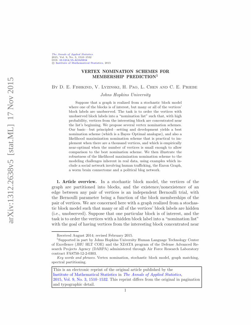
arX

iv:1

312.

2638

v5 [

stat

.ML

] 1

7 N

ov 2

015

The Annals of Applied Statistics

2015, Vol. 9, No. 3, 1510–1532DOI: 10.1214/15-AOAS834c© Institute of Mathematical Statistics, 2015

VERTEX NOMINATION SCHEMES FOR

MEMBERSHIP PREDICTION1

By D. E. Fishkind, V. Lyzinski, H. Pao, L. Chen and C. E. Priebe

Johns Hopkins University

Suppose that a graph is realized from a stochastic block modelwhere one of the blocks is of interest, but many or all of the vertices’block labels are unobserved. The task is to order the vertices withunobserved block labels into a “nomination list” such that, with highprobability, vertices from the interesting block are concentrated nearthe list’s beginning. We propose several vertex nomination schemes.Our basic—but principled—setting and development yields a bestnomination scheme (which is a Bayes–Optimal analogue), and also alikelihood maximization nomination scheme that is practical to im-plement when there are a thousand vertices, and which is empiricallynear-optimal when the number of vertices is small enough to allowcomparison to the best nomination scheme. We then illustrate therobustness of the likelihood maximization nomination scheme to themodeling challenges inherent in real data, using examples which in-clude a social network involving human trafficking, the Enron Graph,a worm brain connectome and a political blog network.

1. Article overview. In a stochastic block model, the vertices of thegraph are partitioned into blocks, and the existence/nonexistence of anedge between any pair of vertices is an independent Bernoulli trial, withthe Bernoulli parameter being a function of the block memberships of thepair of vertices. We are concerned here with a graph realized from a stochas-tic block model such that many or all of the vertices’ block labels are hidden(i.e., unobserved). Suppose that one particular block is of interest, and thetask is to order the vertices with a hidden block label into a “nomination list”with the goal of having vertices from the interesting block concentrated near

Received August 2014; revised February 2015.1Supported in part by Johns Hopkins University Human Language Technology Center

of Excellence (JHU HLT COE) and the XDATA program of the Defense Advanced Re-search Projects Agency (DARPA) administered through Air Force Research Laboratorycontract FA8750-12-2-0303.

Key words and phrases. Vertex nomination, stochastic block model, graph matching,spectral partitioning.

This is an electronic reprint of the original article published by theInstitute of Mathematical Statistics in The Annals of Applied Statistics,2015, Vol. 9, No. 3, 1510–1532. This reprint differs from the original in paginationand typographic detail.

1

2 D. E. FISHKIND ET AL.

the beginning of the list. Forming such a nomination list can be assisted byany available knowledge about the underlying model parameters, as well asby utilizing knowledge of block membership for any of the vertices for whichsuch block labels are observed. A vertex nomination scheme is a functionthat, to each such possible observed graph, assigns an associated nominationlist. In this paper we present, analyze, and illustrate the effectiveness of sev-eral vertex nomination schemes. Some of these vertex nomination schemesutilize graph matching and spectral partitioning machinery. See Copper-smith (2014), Coppersmith and Priebe (2012) and Lee and Priebe (2012)for recent work on vertex nomination, as well as a survey of closely relatedproblems.

One illustrative example of vertex nomination would be a social networkwith vertices representing people, some of whom are engaged in human traf-ficking, the rest of whom are not engaged in human trafficking, and withedges representing a working relationship between the individuals. Law en-forcement may have as a priority separating human trafficking from mun-dane sex work, because not all illegal acts represent the same level of overallcoercion. If several of these people are known to law enforcement as humantraffickers, several are known to law enforcement to not be human traffick-ers, and there are very limited resources to scrutinize the remainder as yetambiguous people to see if they are human traffickers, then a task would beto use the available information and the adjacencies so as to order the as yetambiguous vertices into a nomination list that would prioritize these verticesfor this further scrutiny through other investigative means. In particular, thenomination task here is a task which is not simply classification—it is prior-itization. Later, in Section 9, we highlight a much more elaborate real-dataapplication of vertex nomination in a social network involving actual humantrafficking.

In Section 2 we formally and carefully define the setting and the conceptof a vertex nomination scheme. Although prioritization is a ubiquitous needthat can be treated in an ad hoc fashion specific to individual applications,we here formally set the problem in the stochastic block model setting,which has gained so much popularity in recent literature [e.g., see Airoldiet al. (2009), Bickel and Chen (2009), Nowicki and Snijders (2001)] and is auseful model for real data. This formal setting will be useful for principleddevelopment of techniques that have solid theoretical foundations and arealso robust to the modeling challenges inherent in real data.

In Section 3 we introduce the canonical vertex nomination scheme. It isanalogous to the Bayes classifier in the setting of classification. Indeed, weprove in Proposition 1 that the canonical vertex nomination scheme is atleast as effective as every other vertex nomination scheme, and it thus servesthe valuable role of a “gold standard” with which to gauge the success of

VERTEX NOMINATION 3

other vertex nomination schemes. However, it is computationally practicalto implement only when there are on the order of a very few tens of vertices.

In Section 4 we introduce the likelihood maximization vertex nominationscheme, which fundamentally utilizes graph matching machinery. The graphmatching problem is to find a bijection between the vertex sets of two graphsthat minimizes the number of induced adjacency disagreements; there is avast literature dedicated to this problem, for example, see the article ThirtyYears of Graph Matching in Pattern Recognition [Conte et al. (2004)] foran excellent survey. Although graph matching is intractable in theory, therehave been recent advances in approximate graph matching algorithms thatare both tractable and effective; for example, see Lyzinski, Fishkind andPriebe (2014), Vogelstein et al. (2015) and Zaslavskiy, Bach and Vert (2009).In particular, the very recent SGM algorithm of Lyzinski, Fishkind andPriebe (2014) has been shown in Lyzinski et al. (2015b) to be theoreticallyand practically superior to convex relaxation approaches. Using the SGMalgorithm of Lyzinski, Fishkind and Priebe (2014) for approximate graphmatching, the likelihood maximization vertex nomination scheme is practicalto implement for on the order of 1000 vertices. In Sections 8.1, 8.2 and 8.3, weillustrate the robustness of the likelihood maximization vertex nominationscheme to the model misspecifications inherent in real data. Furthermore,we demonstrate in Section 7 that likelihood maximization performs nearlyas well as the canonical “gold standard”—on graphs that have few enoughvertices so that canonical is indeed computable.

In Section 5 we introduce the spectral partitioning vertex nominationscheme; it is practical to implement for tens of thousands of vertices ormore. Based on the results in Sussman et al. (2012) and Fishkind et al.(2013), then followed up in Lyzinski et al. (2014b), the spectral partitioningvertex nomination scheme nominates perfectly as the number of verticesgoes to infinity, under mild conditions.

In Section 7 we perform illustrative simulations at three different scales,that is, a “small scale” experiment with ten ambiguous vertices, a “mediumscale” experiment with 500 ambiguous vertices, and a “large scale” experi-ment with 10,000 ambiguous vertices. With respect to nomination effective-ness and practicality of implementation, the canonical vertex nominationscheme dominates at the small scale, the likelihood maximization schemedominates at the medium scale, and the spectral partitioning scheme dom-inates at the large scale.

In Section 8.1 we illustrate our vertex nomination schemes on the “EnronGraph,” a graph with email addresses of former employees of the failed En-ron Corporation as vertices, and edges indicating email contact between theassociated vertices over a time interval. Our vertex nomination schemes areused to nominate higher-echelon former Enron employees. Then, in Sections8.2 and 8.3 we illustrate on examples with a worm-brain connectome (to

4 D. E. FISHKIND ET AL.

nominate motor neurons) and a blog network (to nominate political affilia-tion).

In Section 9 we illustrate the impact of our vertex nomination machineryon a real-data social network involving human trafficking. The data are as-sociated with the DARPA Memex and XDATA programs. We have a graphof web advertisements, some of them with known association to human traf-ficking. Using the machinery developed in this manuscript, we were able tonominate ambiguous advertisements for human trafficking in a manner thatwas operationally significant.

2. Vertex nomination schemes; setting and definition. In this article weassume for simplicity that graphs are simple (i.e., edges are not directed,there are no parallel edges and no single-edge loops), but much of what wedo is generalizable.

We begin by describing the stochastic block distribution SB(K,m,n, b,Λ),which will be our random graph setting; its parameters are a positive in-teger K (the number of blocks), a nonnegative integer m (the number ofseeds), a positive integer n (the number of ambiguous vertices), an arbitrarybut fixed function b : {1,2, . . . ,m+n}→ {1,2, . . . ,K} (the block membership

function) and a symmetric matrix Λ ∈ [0,1]K×K (the adjacency probabil-

ities). A random graph with distribution SB(K,m,n, b,Λ) has the vertexset W := {1,2, . . . ,m+ n} and, for each unordered pair of distinct vertices

{w,w′} ∈(W2

)

, w is adjacent to w′ (w ∼ w′) according to an independentBernoulli trial with parameter Λb(w),b(w′).

The vertex set W is partitioned into two sets, the set U := {1,2, . . . ,m}(the seeds) and the set V := {m+1,m+ 2, . . . ,m+ n} (the ambiguous ver-

tices). For each i = 1,2, . . . ,K, define mi := |{u ∈ U : b(u) = i}| and ni :=|{v ∈ V : b(v) = i}|. The function b is only partially observed; its valuesare known on U , but not on V . In other words, the block memberships ofthe seeds are known, and the block memberships of the ambiguous verticesare unknown, but we will assume for simplicity that Λ is known, and thatn1, n2, . . . , nK are known. Given a random graph from SB(K,m,n, b,Λ), themost general inferential task would be to estimate b on W , but we will finetune this task very soon. (Note that if Λ and n1, n2, . . . , nK were not knownthen, if there are enough seeds, Λ could be approximated from edge densi-ties of subgraphs induced by various subsets of the seeds and, in addition,the values of n1, n2, . . . , nK might be approximated if it just so happens tobe known that they are roughly proportional to the respective values ofm1,m2, . . . ,mK . Of course, m1,m2, . . . ,mK are known by virtue of the factthat b is known on U .)

Define Ξ to be the set of bijective functions from W to W that fix theelements of U ; of course, |Ξ|= n!. Any two graphs G and H on the vertex

VERTEX NOMINATION 5

set W are called equivalent if G is isomorphic to H under some functionξ ∈ Ξ; if G is also asymmetric (i.e., its automorphism group is trivial), thensuch a ξ is unique to G,H , denote it ξG,H . For any graph G on vertex setW , the equivalence class of equivalent-to-G graphs on vertex set W will bedenoted 〈G〉; in particular, 〈G〉 is an event. The set of all such equivalenceclasses is denoted Θ; the events in Θ partition the sample space.

A vertex nomination scheme Φ is a mapping that, to each asymmetricgraph G with vertex set W , associates a linear ordering of the vertices in V—called the nomination order, and denoted as a list (ΦG(1),ΦG(2), . . . ,ΦG(n))—such that for everyH equivalent to G it holds that (ξG,H(ΦG(1)), ξG,H(ΦG(2)),. . . , ξG,H(ΦG(n))) = (ΦH(1),ΦH(2), . . . ,ΦH(n)). In other words, and descri-bed somewhat informally, if each equivalence class of graphs is viewed as a(single) graph whose vertex set is comprised of labeled vertices U and unla-beled vertices V , then to each equivalence class (i.e., partially vertex-labeledgraph) Φ associates a list of unlabeled vertices of V .

Note that the fraction of all graphs on vertex set W which are symmetricgoes very quickly to zero as |W | goes to infinity [Erdos and Renyi (1963),Polya (1937)]. Although symmetric graphs are thus negligibly many, it ishelpful for notation to extend the domain of Φ to include symmetric graphs,and this can be done in many different ways. For simplicity of analysis wewill simply say for now that, to every symmetric graph G on the vertex setW , the associated nomination list is declared to be (m+1,m+2, . . . ,m+n)(and we do not require the nomination list in this case to meet the propertymentioned above).

In this article, we assume that only membership in the first block is ofinterest; the specific task we are concerned with is to find vertex nominationschemes under which there will be, with high probability, an abundance ofmembers of the first block that are near the beginning of the nominationlist. As an illustrative example related to the Enron Graph example in Sec-tion 8.1, consider a corporation with m+n=m1+m2+n1+n2 employees,of which m1 + n1 are involved in fraud and m2 + n2 are not involved infraud. The probability of communication between fraudsters is fixed, as isthe probability of communication between nonfraudsters, as is the probabil-ity of communication between any fraudster and any nonfraudster. Of them1 + n1 fraudsters, m1 have been identified as fraudsters and, among them2 + n2 nonfraudsters, m2 have been identified as nonfraudsters. Based onobserving all of the employee communications (together with knowledge ofthe identities of m1 fraudsters and m2 nonfraudsters), we wish to draw up anomination list of the n1 +n2 ambiguous employees so that there are manyfraudsters early in the list.

The effectiveness of a vertex nomination scheme Φ is quantified in thefollowing manner. For any graph G with vertex set W , and for any in-teger j such that 1 ≤ j ≤ n, the precision at depth j of Φ for G is de-

fined to be |{1≤i≤j:b(ΦG(i))=1}|j ; for the corporate illustration, this represents

6 D. E. FISHKIND ET AL.

the fraction of the first j employees on the nomination list that are ac-tual fraudsters in truth. The average precision of Φ for G is defined to be1n1

∑n1j=1

|{1≤i≤j:b(ΦG(i))=1}|j ; it has a value between 0 (per the corporate ex-

ample, if none of the first n1 nominated employees are fraudsters) and 1(if all of the first n1 nominated employees are fraudsters). Note that theaverage precision of Φ for G is equal to

∑n1i=1(

1n1

∑n1j=i

1j )δb(ΦG(i))=1, where δ

is the usual indicator function. In particular, the average precision of Φ forG is a convex combination of the indicators δb(ΦG(i))=1, with more weightin this convex combination for indicators associated with lower values ofi. The mean average precision of the vertex nomination scheme Φ is theexpected value of the average precision for a random graph G distributedSB(K,m,n, b,Λ). The closer that this number is to 1, the more effective avertex nomination scheme Φ is deemed. Note that a “chance” vertex nomi-nation scheme would have the value n1

n as its mean average precision.We point out that our definition of average precision is slightly different

than a definition commonly used in the information retrieval community;our definition is a pure average precision, whereas the other definition isactually an integral of the precision over recall.

3. The canonical vertex nomination scheme. In this section we definethe canonical vertex nomination scheme, which is analogous to the Bayesclassifier in the Bayes classifier’s setting of classification. Indeed, we provein Proposition 1 that the mean average precision of the canonical vertexnomination scheme is greater than or equal to the mean average precisionof every other vertex nomination scheme. Unfortunately, because of its com-putational intractability (a visibly exponential runtime as the number ofvertices increases), the canonical vertex nomination scheme is only practi-cal to implement for up to a few tens of vertices. Nonetheless, because ofProposition 1, the canonical vertex nomination scheme serves as a valuable“gold standard” to evaluate the performance of other more computationallytractable vertex nomination schemes. (This is analogous to the role of theBayes classifier in the classification setting.) Our ongoing research seeks toapproximate the canonical vertex nomination scheme in a scalable fashion.

3.1. Definition of the scheme. Consider the random graph G distributedSB(K,m,n, b,Λ). When G is asymmetric then, for any v ∈ V , the conditionalprobability

P[{H ∈ 〈G〉 : b(ξG,H(v)) = 1}|〈G〉](1)

may be described as the probability, given the event that we observe agraph equivalent to G, that the vertex corresponding to v would be in thefirst block. The canonical vertex nomination scheme, which we denote as

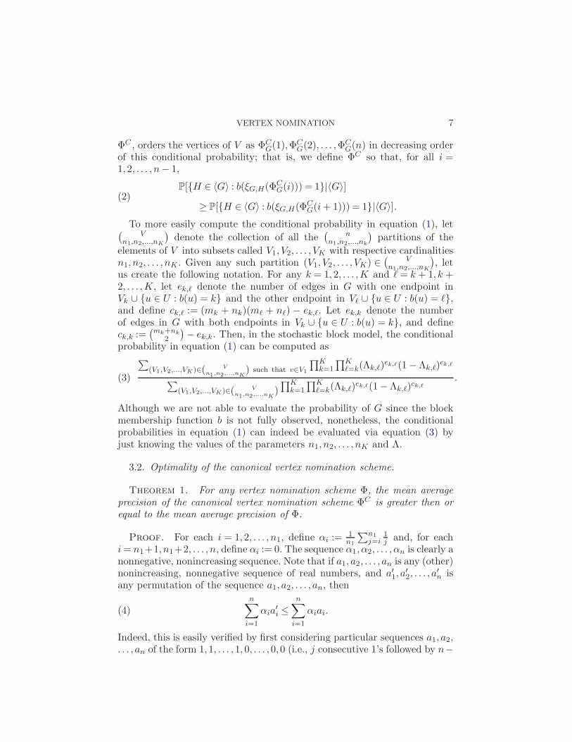
VERTEX NOMINATION 7

ΦC , orders the vertices of V as ΦCG(1),Φ

CG(2), . . . ,Φ

CG(n) in decreasing order

of this conditional probability; that is, we define ΦC so that, for all i =1,2, . . . , n− 1,

P[{H ∈ 〈G〉 : b(ξG,H(ΦCG(i))) = 1}|〈G〉]

(2)≥ P[{H ∈ 〈G〉 : b(ξG,H(ΦC

G(i+ 1))) = 1}|〈G〉].

To more easily compute the conditional probability in equation (1), let(

Vn1,n2,...,nK

)

denote the collection of all the(

nn1,n2,...,nk

)

partitions of the

elements of V into subsets called V1, V2, . . . , VK with respective cardinalitiesn1, n2, . . . , nK . Given any such partition (V1, V2, . . . , VK) ∈

(

Vn1,n2,...,nK

)

, letus create the following notation. For any k = 1,2, . . . ,K and ℓ= k + 1, k +2, . . . ,K, let ek,ℓ denote the number of edges in G with one endpoint inVk ∪ {u ∈ U : b(u) = k} and the other endpoint in Vℓ ∪ {u ∈ U : b(u) = ℓ},and define ck,ℓ := (mk + nk)(mℓ + nℓ) − ek,ℓ. Let ek,k denote the numberof edges in G with both endpoints in Vk ∪ {u ∈ U : b(u) = k}, and defineck,k :=

(mk+nk

2

)

− ek,k. Then, in the stochastic block model, the conditionalprobability in equation (1) can be computed as

∑

(V1,V2,...,VK)∈( V

n1,n2,...,nK) such that v∈V1

∏Kk=1

∏Kℓ=k(Λk,ℓ)

ek,ℓ(1−Λk,ℓ)ck,ℓ

∑

(V1,V2,...,VK)∈( Vn1,n2,...,nK

)∏K

k=1

∏Kℓ=k(Λk,ℓ)

ek,ℓ(1−Λk,ℓ)ck,ℓ

.(3)

Although we are not able to evaluate the probability of G since the blockmembership function b is not fully observed, nonetheless, the conditionalprobabilities in equation (1) can indeed be evaluated via equation (3) byjust knowing the values of the parameters n1, n2, . . . , nK and Λ.

3.2. Optimality of the canonical vertex nomination scheme.

Theorem 1. For any vertex nomination scheme Φ, the mean average

precision of the canonical vertex nomination scheme ΦC is greater then or

equal to the mean average precision of Φ.

Proof. For each i = 1,2, . . . , n1, define αi :=1n1

∑n1j=i

1j and, for each

i= n1+1, n1+2, . . . , n, define αi := 0. The sequence α1, α2, . . . , αn is clearly anonnegative, nonincreasing sequence. Note that if a1, a2, . . . , an is any (other)nonincreasing, nonnegative sequence of real numbers, and a′1, a

′2, . . . , a

′n is

any permutation of the sequence a1, a2, . . . , an, thenn∑

i=1

αia′i ≤

n∑

i=1

αiai.(4)

Indeed, this is easily verified by first considering particular sequences a1, a2,. . . , an of the form 1,1, . . . ,1,0, . . . ,0,0 (i.e., j consecutive 1’s followed by n−

8 D. E. FISHKIND ET AL.

j consecutive 0’s, for different values of j = 1,2, . . . , n) and then noting thatthe nonnegative combinations of such particular sequences indeed compriseall nonincreasing, nonnegative sequences with n entries.

Consider the random graph G distributed SB(K,m,n, b,Λ). Recall thatΘ denotes the set of equivalence classes of graphs on the vertex set W .

Expanding the mean average precisions of Φ, then bounding and simpli-fying, yields

E

(

n∑

i=1

αiδb(ΦG(i))=1

)

=

n∑

i=1

αiP(b(ΦG(i)) = 1)

=n∑

i=1

αi

(

∑

G∈Θ

P(G)P(b(ΦG(i)) = 1∣

∣

∣G)

)

=∑

G∈Θ

P(G)

(

n∑

i=1

αiP(b(ΦG(i)) = 1∣

∣

∣G)

)

(5)

≤∑

G∈Θ

P(G)

(

n∑

i=1

αiP(b(ΦCG(i)) = 1

∣

∣

∣G)

)

=n∑

i=1

αiP(b(ΦCG(i)) = 1) = E

(

n∑

i=1

αiδb(ΦCG(i))=1

)

,

where the inequality in equation (5) follows from equations (4) and (2),(and from our assumption that all nomination schemes agree when G issymmetric). The desired result is shown. �

4. Likelihood maximization vertex nomination scheme. In this sectionwe define the likelihood maximization vertex nomination scheme. It willbe practical to implement even when there are on the order of a thousandvertices. We will see in Section 7 that it is a very effective vertex nominationscheme, when compared to the canonical vertex nomination scheme “goldstandard” on graphs small enough to make the comparison. In Sections 8.1,8.2 and 8.3 we will see that likelihood maximization appears to be nicelyrobust to the modeling challenges inherent in real data.

4.1. Definition of the scheme. Suppose the random graph G is distributedSB(K,m,n, b,Λ). There are two stages in defining—and computing—thelikelihood maximization vertex nomination scheme.

The first stage is concerned with estimating the block assignment functionb. Let B denote the set of functions b :W →{1,2, . . . ,K} such that b agreeswith b on U , and such that it also holds, for all i= 1,2, . . . ,K, that |{v ∈ V :

VERTEX NOMINATION 9

b(v) = i}|= ni. For any b ∈B, and for all k = 1,2, . . . ,K and ℓ= k+1, k+2,. . . ,K, let ek,ℓ(b) denote the number of edges in G with one endpoint in {w ∈W : b(w) = k} and the other endpoint in {w ∈W : b(w) = ℓ}, and also denoteck,ℓ(b) := (mk + nk)(mℓ + nℓ) − ek,ℓ(b). For all k = 1,2, . . . ,K, let ek,k(b)denote the number of edges in G with both endpoints in {w ∈W : b(w) =k}, and also denote ck,k(b) :=

(

mk+nk

2

)

− ek,k(b). In the SB(K,m,n, b,Λ)distribution, if b had been replaced with b ∈ B, then the probability ofrealizing the graph G would have been

p(b,G) :=

K∏

k=1

K∏

ℓ=k

(Λk,ℓ)ek,ℓ(b)(1−Λk,ℓ)

ck,ℓ(b).(6)

Define b, the maximum likelihood estimator of b, to be the member of Bsuch that the probability of G is maximized. In other words (then takinglogarithms and ignoring additive constants),

b := argmaxb∈B

p(b,G) = argmaxb∈B

K∑

k=1

K∑

ℓ=k

ek,ℓ(b) log

(

Λk,ℓ

1−Λk,ℓ

)

(7)

= argmaxb∈B

∑

{w,w′}∈(W2 )

δw∼Gw′ log

(

Λb(w),b(w′)

1−Λb(w),b(w′)

)

.

The optimization problem in equation (7) is an example of seeded graphmatching, and we can efficiently and effectively approximate its solution.The details of this are deferred to the next section, Section 4.2, and wenow continue on to the second stage of defining and computing the likeli-hood maximization vertex nomination scheme, assuming that we have com-puted b.

For any v, v′ ∈ V such that b(v) = 1 and b(v′) 6= 1, define bv↔v′ ∈ B

such that bv↔v′ agrees with b for all w ∈W except that bv↔v′(v′) = 1 and

bv↔v′(v) = b(v′). For any v, v′ ∈ V such that b(v) = 1 and b(v′) 6= 1, we can

interpret a low/high value of the quantityp(bv↔v′ ,G)

p(b,G)as a measure of our

conviction/lack-of-conviction that b should be used to estimate b, as op-

posed to estimating b with specifically bv↔v′ . In this spirit, for all v ∈ V

such that b(v) = 1, a low/high value of the geometric mean

(

∏

v′∈V :b(v′)6=1

p(bv↔v′ ,G)

p(b,G)

)1/(n−n1)

(8)

can be interpreted as a measure (for the purpose of ordering) of our convic-tion/

10 D. E. FISHKIND ET AL.

lack-of-conviction in our estimation that b(v) is 1. Also, for all v′ ∈ V such

that b(v′) 6= 1, a low/high value of the geometric mean(

∏

v∈V :b(v)=1

p(bv↔v′ ,G)

p(b,G)

)1/n1

(9)

can be interpreted as a measure (just for the purpose of ordering) of ourconviction/lack-of-conviction in our estimation that b(v′) is not 1.

We now define the likelihood maximization vertex nomination scheme ΦL

to be such that it satisfies ΦLG(1),Φ

LG(2), . . . ,Φ

LG(n1) are the v ∈ V such that

b(v) = 1, listed in increasing order of the geometric mean in equation (8),

and ΦLG(n1 + 1),ΦL

G(n1 + 2), . . . ,ΦLG(n) are the v′ ∈ V such that b(v′) 6= 1,

listed in decreasing order of the geometric mean in equation (9).

4.2. Solving the seeded graph matching problem. In this section we dis-cuss how to compute b in the likelihood maximization vertex nominationscheme ΦL defined in the previous section.

Given any A,B ∈R(m+n)×(m+n), the quadratic assignment problem is to

minimize ‖A−PBP T‖2F over all permutation matrices P ∈ {0,1}(m+n)×(m+n) ,where ‖·‖F denotes the Frobenius matrix norm. If A and B are, respectively,adjacency matrices for two graphs, then this is called the graph matching

problem; it is clearly equivalent to finding a bijection from the vertex setof one graph to the vertex set of the other graph so as to minimize thenumber of adjacency disagreements induced by the bijection. If P is furtherconstrained so that the upper left corner is the m×m identity matrix, thenthe problem is called the seeded quadratic assignment problem/seeded graph

matching problem; for graphs, this further restriction just means that partof the bijection between the vertex sets is fixed.

Note that the objective function can be simplified (under the restric-tion that P is a permutation matrix) as ‖A− PBP T‖2F = ‖A‖2F + ‖B‖2F −2〈A,PBP T 〉, where 〈·, ·〉 is the usual inner product 〈C,D〉 :=

∑

i,j CijDij .

Thus, the above problems can be phrased as maximize 〈A,PBP T 〉 over allpermutation matrices P .

The optimization problem in equation (7), for which b is the solution,is precisely the seeded quadratic assignment problem above, where A ∈R(m+n)×(m+n) is the adjacency matrix for the graph G, that is, Ai,j := δi∼Gj

for all i, j ∈ W ≡ {1,2, . . . ,m + n}, and B ∈ R(m+n)×(m+n) is the matrix

wherein Bi,j := log(Λb′(i),b′(j)

1−Λb′(i),b′(j)

) for all i, j ∈W , where b′ is the member of

B for which the sequence b′(m+1),b′(m+2), . . . ,b′(m+n) are 1’s contigu-ously, then 2’s contiguously, . . . , then K’s contiguously. The b ∈ B—overwhich the objective function in equation (7) is maximized—correspond pre-cisely to the permutation matrices P in the seeded quadratic assignment

VERTEX NOMINATION 11

problem, where the upper left corner of P is restricted to be the m ×m

identity matrix. We will call this problem a seeded graph matching problembecause A is an adjacency matrix. (And we can also choose to think of Bas a weighted adjacency matrix for a graph.)

The seeded graph matching problem is computationally hard; indeed,the quadratic assignment problem is NP-hard, and even deciding if twographs are isomorphic is notoriously of unknown complexity [Garey andJohnson (1979), Read and Corneil (1977)]. However, approximate solutionscan be found efficiently with the SGM (Seeded Graph Matching) Algorithmof Lyzinski, Fishkind and Priebe (2014), which is a seeded version of theFAQ algorithm of Vogelstein et al. (2015). [Indeed, SGM is more effectivethan convex relaxation techniques, as was recently shown in Lyzinski et al.(2015b).] We employ the SGM algorithm to obtain an approximate solution

to b for use in the likelihood maximization vertex nomination scheme. Itruns in time O(n3), and can be implemented even when n is approximately1000.

5. The spectral partitioning vertex nomination scheme. In this sectionwe introduce the spectral partitioning vertex nomination scheme. SupposeG is distributed SB(K,m,n, b,Λ). We do not need to assume here that weknow n1, n2, . . . , nK , nor the entries of Λ; we just need to know the value ofK and d := the rank of Λ. [Indeed, by the results in Fishkind et al. (2013),even just knowing an upper bound on d will be sufficient to obtain goodperformance.]

Say that the adjacency matrix for G is A ∈ {0,1}(m+n)×(m+n) , that is,Ai,j := δi∼Gj for all i, j ∈ W ≡ {1,2, . . . ,m + n}. Compute d eigenvectorsassociated, respectively, with the d largest-modulus eigenvalues of A. Scalethese eigenvectors so that their respective lengths are the square roots of theabsolute values of their corresponding eigenvalues, and define X ∈R

(m+n)×d

to have these scaled eigenvectors as its respective columns. The rows of Xare low-dimensional embeddings of the corresponding vertices. Now, clusterthe rows of X into K clusters; that is, solve the problem minimize ‖X−C‖Fover all matrices C ∈R

(m+n)×d with the property that each row of C is equalto one of just K row vectors, and the values of these K row vectors are alsovariables to be optimized over.

Say that c is the most frequent value of row vector in the optimal C amongthe rows corresponding to the vertices {u ∈ U : b(u) = 1}. (In other words,c is the centroid associated with the most vertices known to be in the firstblock.) The spectral partitioning vertex nominating scheme, denoted by ΦS ,associates with G the ordering (of vertices in V ) ΦS

G(1),ΦSG(2), . . . ,Φ

SG(n)

in increasing order of Euclidean distance between c and their correspondingrow in X .

12 D. E. FISHKIND ET AL.

Suppose we consider a sequence of graphs realized from the distributionsSB(K,m,n, b,Λ) for, successively, m + n = 1,2,3, . . . , where K and Λ arefixed, and Λ is positive semi-definite with the property that no two of itsrows are equal. Also, assume thatm1 ≥ 1, and there exists a positive constantγ such that, for all i= 1,2, . . . ,K, it holds that mi +ni ≥ γ(m+n)3/4+γ . Itwas recently shown in Lyzinski et al. (2014b) [following the work in Sussmanet al. (2012) and Fishkind et al. (2013)] that almost surely there are noincorrectly clustered vertices in the limit. This implies that the mean averageprecision of ΦS converges to 1 as m+ n→∞.

It will be computationally convenient to approximately (but very quickly)solve the clustering subproblem. This approximate clustering can be donewith the k-means algorithm or with the mclust procedure [Fraley and Raftery(1999, 2003)]. In both cases, the vertices are nominated based on distance tocluster centroids; in k-means this amounts to the usual Euclidean distance,while for mclust this amounts to nominating based on the Mahalonobis dis-tance.

6. The OTS vertex nomination scheme. The chief contribution of thismanuscript is the formulation of the likelihood maximization vertex nomi-nation scheme, along with our demonstration of its effectiveness; indeed, itis comparably effective to the “gold standard” canonical vertex nominationscheme (on graphs small enough to practically make this comparison, as wedemonstrate in Section 7) and it is relatively robust to pathologies inherentin real data (as we demonstrate later in Section 8).

However, it is worthwhile to point out that classification algorithms forstochastic block models can often be naturally modified for use in nom-ination, by utilizing algorithm-inherent numeric scores to perform vertexranking. For an excellent survey of the literature on community detectionin networks—including the setting of stochastic block models—and avail-able algorithms, see the very comprehensive survey article Fortunato (2010)and the papers cited therein, such as Newman and Girvan (2004) and theclassic article Nowicki and Snijders (2001). Also, see Latent Dirichlet Al-location (LDA) [Blei, Ng and Jordan (2003)]. Because of the vast num-ber of citations to it in the literature, we next choose to focus on thepaper Airoldi et al. (2009), titled “Mixed membership stochastic block-models,” and the associated R code which we call “MMSB” located athttp://cran.r-project.org/web/packages/lda/lda.pdf [Chang and Dai (2010)];in the setting of a mixed membership block model, MMSB assigns to eachvertex a posterior probability of block membership in each of the variousblocks. With this, we now define the OTS vertex nomination scheme, de-noted ΦO, which uses MMSB to order the vertices of V in decreasing orderof posterior probability of membership in the specific block indicated by themost seeds.

VERTEX NOMINATION 13

We call this nomination scheme OTS “Off The Shelf” to emphasize thatwe use MMSB as a black box without getting under the hood of the code;as such, the use of the seeds is only to identify the block of interest. Indeed,under the hood modifications of existing community detection algorithmssuch as MMSB and LDA and LDA-based methodologies are expected toyield new vertex nomination schemes that will be increasingly effective andfast. We also expect even more effective vertex nomination schemes to comefrom merging vertex nomination techniques, perhaps similar in spirit tothe work in Lyzinski et al. (2015a), where graph matching and spectralpartitioning are merged into a more effective avenue of graph matching forlarge graphs.

7. Simulations: Comparing the vertex nomination schemes at three dif-

ferent scales. In this section we compare and contrast these vertex nomina-tion schemes using three simulation experiments—essentially the same ex-periment at three different scales, “small scale,” “medium scale” and “largescale.” For each of the three experiments, we have K = 3 blocks in thestochastic block model. The matrix of Bernoulli parameters Λ is

Λ(ϑ) := ϑ

0.5 0.3 0.4

0.3 0.8 0.6

0.4 0.6 0.3

+ (1− ϑ)

0.5 0.5 0.5

0.5 0.5 0.5

0.5 0.5 0.5

,

with the value ϑ= 1 for the small scale experiment, ϑ= 0.3 for the mediumscale experiment, and ϑ = 0.1 for the large scale experiment, in order todecrease the signal when the number of vertices is larger.

Specifically, the matrix Λ for the small scale experiment, for the mediumscale experiment and for the large scale experiment are, respectively,

Λ(1) =

0.5 0.3 0.4

0.3 0.8 0.6

0.4 0.6 0.3

, Λ(0.3) =

0.50 0.44 0.47

0.44 0.59 0.53

0.47 0.53 0.44

,

Λ(0.1) =

0.50 0.48 0.49

0.48 0.53 0.51

0.49 0.51 0.48

,

so that as the number of vertices increases we have that ϑ gets closer to zero,which means that the blocks become less and less stochastically differentiableone from the other. Another notable feature of the Λ here is that the blockof interest—the first block—is the intermediate density block, that is, theBernoulli adjacency parameter for vertices in the first block is between theBernoulli adjacency parameter for vertices in the second block and in thethird block. This makes it more challenging to identify the vertices of thefirst block, which is the block of interest.

14 D. E. FISHKIND ET AL.

The values of (n1, n2, n3) are taken to be multiples of (4,3,3), specifically,in the small-scale experiment (n1, n2, n3) = (4,3,3), in the medium-scaleexperiment (n1, n2, n3) = (200,150,150) and in the large-scale experiment(n1, n2, n3) = (4000,3000,3000). As for the seeds, the values of (m1,m2,m3)in the respective experiments were taken as (4,0,0), (20,0,0) and(40,0,0).

These three experiments were performed as follows. We independentlyrealized 50,000 graphs from the associated distribution of the small-scaleexperiment, 200 graphs in the medium-range experiment and 100 graphsin the large-scale experiment. To each observed graph we applied each ofthe following: the canonical vertex nomination scheme ΦC , the likelihoodmaximization vertex nomination scheme ΦL, the OTS vertex nominationscheme ΦO and the spectral partitioning vertex nomination scheme ΦS .Then, for each vertex nomination scheme, we recorded the fraction of therealizations for which the first nominee of the nomination list was a mem-ber of the block of interest, the fraction of the realizations for which thesecond nominee was a member of the block of interest, . . . , the fraction ofthe realizations for which the nth nominee was a member of the block ofinterest. In Figure 1(a), (b) and (c) these empirical probabilities are plottedagainst nomination list position, for the three respective experiments andthe nomination schemes.

In the small-scale experiment, where n= 10, the likelihood maximizationnomination scheme performed about as well as the (“gold standard”) canon-ical nomination scheme, and the spectral partitioning nomination schemeperformed very poorly—near chance. Then, in the medium-scale experi-ment, where n= 500, the canonical nomination scheme was no longer prac-tical to compute, and the OTS and the spectral partitioning nominationscheme performed nearly as well as the likelihood maximization nominationscheme. For a few thousand vertices it was not practical to implement thelikelihood maximization nomination scheme nor OTS, so in the large-scaleexperiment, where n = 10,000, the only nomination scheme that could beimplemented was the spectral partitioning nomination scheme.

The empirical mean average precision for the canonical, likelihood maxi-mization and spectral partitioning vertex nomination schemes in the threeexperiments were as follows (note that the mean average precision for chanceis 0.4):

Mean average precision Canonical Likeli-max OTS Spectral

Small-scale exper., n= 10, ϑ= 1 0.6958 0.6725 0.4763 0.3993Medium-scale exper., n= 500, ϑ= 0.3 * 0.9543 0.7846 0.7330Large-scale exper., n= 10,000, ϑ= 0.1 * * * 0.9901

VERTEX NOMINATION 15

(a) Small-scale; n= 10

(b) Medium-scale; n= 500 (c) Large-scale n= 10,000

Fig. 1. The canonical vertex nomination scheme is in red, the likelihood maximizationvertex nomination scheme is in blue, the OTS vertex nomination scheme is in purple,and the spectral partitioning vertex nomination scheme is in green. (Canonical schemenot shown in medium- and large-scale figures, liklihood maximization and OTS schemesnot shown in large-scale figure.)

The running times in seconds were as follows:

Running time per simulation Canonical Likeli-max. OTS Spectral

Small-scale experiment, n= 10 ≈ 0.52 ≈ 0.03 ≈ 0.30 ≈ 0.01Medium-scale experiment, n= 500 * ≈ 332 ≈ 58 ≈ 0.17Large-scale experiment, n= 10,000 * * * ≈ 106

Indeed, each of the canonical, likelihood maximization and spectral vertexnomination schemes is superior (in the sense of effectiveness, given practicalcomputability limitations) to the other two at one of the three scales. Ata small scale you should use the canonical vertex nomination scheme, at amedium scale you should use the likelihood maximization vertex nomination

16 D. E. FISHKIND ET AL.

scheme, and at a large scale you should use the spectral partitioning vertexnomination scheme.

8. Real data examples. While the stochastic block model is often use-ful for modeling real data, many times real data does not fit the modelparticularly well. In the following real-data experiments we see that thelikelihood maximization vertex nomination scheme is robust to the lackof idealized conditions hypothesized and other pathologies inherent in realdata. All of the data and code used in these experiments can be accessed athttp://www.cis.jhu.edu/˜parky/vn/.

8.1. Example: The enron graph. The Enron Corporation was a highly re-garded, large energy company that went spectacularly bankrupt in the early2000s amid systemic internal fraud. Enron has since become a popular exem-plar of corporate fraud and corruption. In the wake of Enron’s collapse, theUS Energy Regulatory Commission collected a corpus of more than 600,000emails sent between Enron employees, and this corpus was made public bythe US Department of Justice and is available online at a number of websites,including http://research.cs.queensu.ca/home/skill/siamworkshop.html.

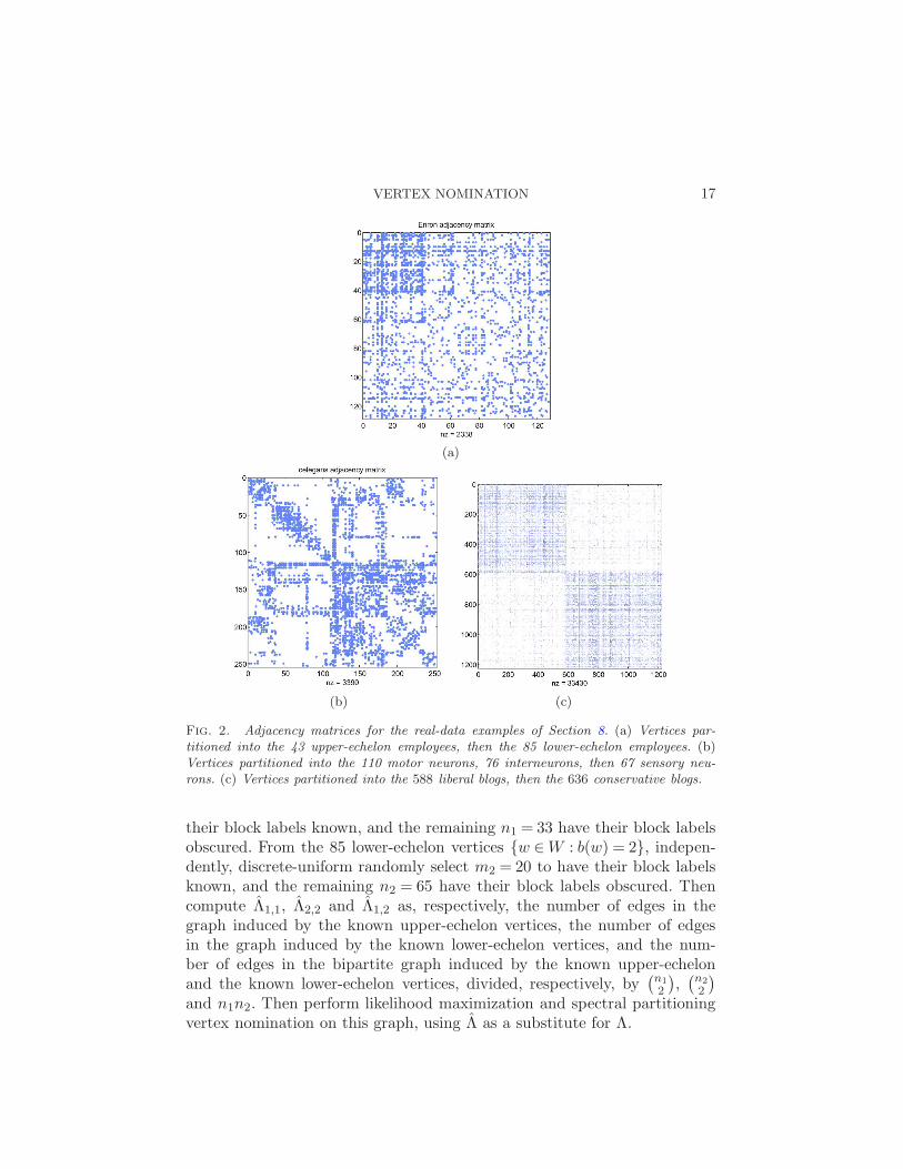
In Priebe et al. (2005), the authors restrict their attention to a 189 weekperiod from the year 1998 through the year 2002; they identify 184 distinctemail addresses in the Enron email corpus over this time interval, and theyidentify the pairs of these email addresses that had email communicationwith each other. Our “Enron Graph” that we use here is based on thegraph in Priebe et al. (2005); our vertex set W consists of the 128 activeemail addresses for which the employee’s job title in Enron was known.For every pair of such vertices, the pair of vertices are declared adjacent toeach other when there was at least one email sent from either of the emailaddresses to the other. We then divided the vertices into two blocks: The“upper-echelon” set of vertices {w ∈ W : b(w) = 1} are the vertices whosejob titles were designated as CEO, president, vice president, chief manager,company attorney and chief employee. The “lower-echelon” set of vertices{w ∈ W : b(w) = 2} are the vertices whose job titles were designated asemployee, employee administrative, specialist, analyst, trader, director andmanager (besides chief manager, which we designated upper echelon). Wechose to group the job titles of manager and director with lower-echelonbecause a by-eye assessment of the graph indicated that their adjacencyaffinity was closer to the rest of the lower-echelon vertices. Indeed, this graphis certainly not a realization of an actual two-block stochastic block model,but for the purpose of illustration we will view it as very roughly havingsome two-block structure. The adjacency matrix is pictured in Figure 2(a).

We consider the following experiment. From the 43 upper-echelon ver-tices {w ∈W : b(w) = 1}, discrete-uniform randomly select m1 = 10 to have

VERTEX NOMINATION 17

(a)

(b) (c)

Fig. 2. Adjacency matrices for the real-data examples of Section 8. (a) Vertices par-titioned into the 43 upper-echelon employees, then the 85 lower-echelon employees. (b)Vertices partitioned into the 110 motor neurons, 76 interneurons, then 67 sensory neu-rons. (c) Vertices partitioned into the 588 liberal blogs, then the 636 conservative blogs.

their block labels known, and the remaining n1 = 33 have their block labelsobscured. From the 85 lower-echelon vertices {w ∈W : b(w) = 2}, indepen-dently, discrete-uniform randomly select m2 = 20 to have their block labelsknown, and the remaining n2 = 65 have their block labels obscured. Thencompute Λ1,1, Λ2,2 and Λ1,2 as, respectively, the number of edges in thegraph induced by the known upper-echelon vertices, the number of edgesin the graph induced by the known lower-echelon vertices, and the num-ber of edges in the bipartite graph induced by the known upper-echelonand the known lower-echelon vertices, divided, respectively, by

(n1

2

)

,(n2

2

)

and n1n2. Then perform likelihood maximization and spectral partitioningvertex nomination on this graph, using Λ as a substitute for Λ.

18 D. E. FISHKIND ET AL.

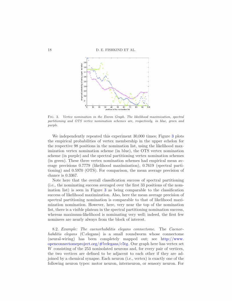
Fig. 3. Vertex nomination in the Enron Graph. The likelihood maximization, spectralpartitioning and OTS vertex nomination schemes are, respectively, in blue, green andpurple.

We independently repeated this experiment 30,000 times; Figure 3 plotsthe empirical probabilities of vertex membership in the upper echelon forthe respective 98 positions in the nomination list, using the likelihood max-imization vertex nomination scheme (in blue), the OTS vertex nominationscheme (in purple) and the spectral partitioning vertex nomination schemes(in green). These three vertex nomination schemes had empirical mean av-erage precisions 0.7779 (likelihood maximization), 0.7619 (spectral parti-tioning) and 0.5970 (OTS). For comparison, the mean average precision ofchance is 0.3367.

Note here that the overall classification success of spectral partitioning(i.e., the nominating success averaged over the first 33 positions of the nom-ination list) is seen in Figure 3 as being comparable to the classificationsuccess of likelihood maximization. Also, here the mean average precision ofspectral partitioning nomination is comparable to that of likelihood maxi-mization nomination. However, here, very near the top of the nominationlist, there is a visible plateau in the spectral partitioning nomination success,whereas maximum-likelihood is nominating very well; indeed, the first fewnominees are nearly always from the block of interest.

8.2. Example: The caenorhabditis elegans connectome. The Caenor -habditis elegans (C.elegans) is a small roundworm whose connectome(neural-wiring) has been completely mapped out; see http://www.openconnectomeproject.org/#!celegans/c5tg. Our graph here has vertex setW consisting of the 253 nonisolated neurons and, for every pair of vertices,the two vertices are defined to be adjacent to each other if they are ad-joined by a chemical synapse. Each neuron (i.e., vertex) is exactly one of thefollowing neuron types: motor neuron, interneuron, or sensory neuron. For

VERTEX NOMINATION 19

each w ∈W , we define the block membership b(w) to be 1,2,3, respectively,according to whether the neuron is a motor neuron (there are 110 of these),interneuron (there are 76 of these) or sensory neuron (there are 67 of these).The adjacency matrix is pictured in Figure 2(b).

Consider the following experiment. Block membership is revealed for 30discrete-uniformly selected motor neurons, 20 discrete-uniformly selectedinterneurons and 10 discrete-uniformly selected sensory neurons. We areinterested in forming a nomination list out of the remaining 193 ambiguousneurons so that the beginning of the nomination list has an abundance of(the remaining 80) ambiguous motor neurons.

Perhaps the story behind your desire for this nomination list might be thatyou wish to study motor neurons, but have limited resources to biochemicallytest neuron type for the ambiguous neurons. The nomination list would beused to order the ambiguous neurons for the testing, to identify as manymotor neurons as possible from the ambiguous neurons before your resourcesare depleted.

We repeated this experiment 1000 times, each time nominating for motorneurons using the likelihood maximization, the spectral partitioning ver-tex nomination scheme and the OTS vertex nomination scheme. In eachrepetition, we estimated Λ with Λ, whose entries reflect the edge densitiesin the subgraphs induced by the various blocks intersecting the seeds. Theempirical mean average precision for the likelihood maximization, spectralpartitioning and OTS vertex nomination schemes were, respectively, 0.7272,0.5096 and 0.5041; the mean average precision of chance is 0.4145. Figure 4shows that empirical probability of being a motor neuron at every positionin the vertex nomination list, for the likelihood maximization (blue), OTS(purple) and spectral partitioning (green) vertex nomination schemes.

Fig. 4. Vertex nomination for motor neurons in C. Elegans: Likelihood maximization iscolored blue, OTS is colored purple, spectral partitioning is colored green.

20 D. E. FISHKIND ET AL.

Note that here spectral partitioning performed very erratically and (over-all) poorly. This might be attributed to a lack of our idealized three-blockstructure here; that is to say, this graph does not appear to be an instan-tiation of monolithic stochastic behavior for vertices within the respectivethree blocks. In this case here, likelihood maximization was seen to be morerobust to the lack of idealized block model setting, and still maintained asteady and very pronounced slope in Figure 4.

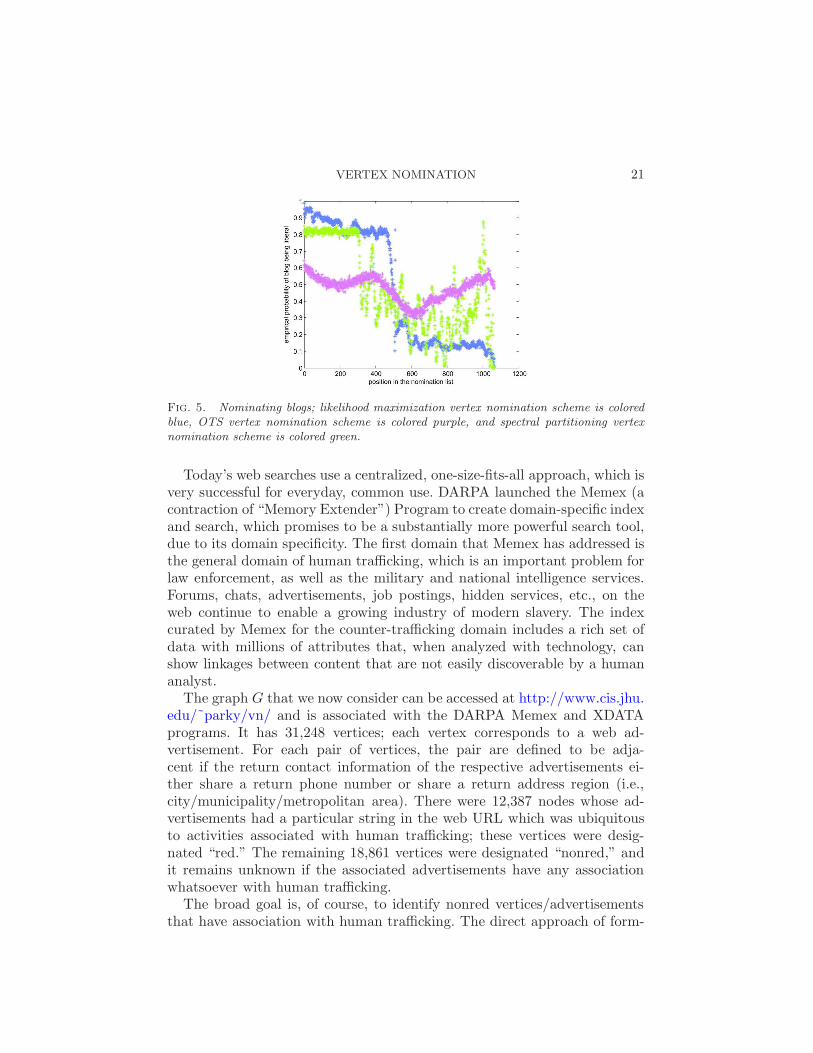
8.3. Example: A political blog network. The political blogosphere datain our next example was collected in Adamic and Glance (2005) around thetime of the US presidential election in 2004. This data set consists of 1224weblogs (“blogs”), each of which web-links to—or is web-linked from—atleast one other of these blogs. These blogs form the vertex set W of ourgraph. Each of the blogs was classified by Adamic and Glance (2005) asbeing either liberal or conservative; for each w ∈ W we define b(w) to be1 or 2, according to whether w was classified as liberal or conservative.There are 588 liberal blogs and 636 conservative blogs here. For each pairof vertices/blogs, the pair is adjacent if at least one of the blogs links to theother. The adjacency matrix is pictured in Figure 2(c).

Consider the following experiment. Discrete-uniform randomly select 80liberal and 80 conservative blogs to have their political orientation revealed,and create a nomination list for the remaining 1064 ambiguous blogs. Thestory could be that you work for a political action committee and wantto make a report summarizing liberal blog views on some current event.You have a limited amount of blog-reading time and only know the contentand political affiliations of a few of the blogs. Thus, you want to create anomination list which will provide the order for your reading the ambiguousblogs, so that you read many liberal blogs in your limited time.

We repeated this experiment 1000 times and calculated the likelihoodmaximization, spectral partitioning and OTS vertex nomination schemesfor each repetition. See the results in Figure 5. The mean average preci-sion for the likelihood maximization, spectral partitioning and OTS vertexnomination schemes were, respectively, 0.8922, 0.7856 and 0.5429; the meanaverage precision for chance nomination was 0.4774.

9. Real-data example: Memex and human-trafficking. The Defense Ad-vanced Research Projects Agency (DARPA) is an agency of the UnitedStates Department of Defense which, historically, was responsible for devel-oping computer networking and NLS (an acronym for “oN-Line System”),which was the first hypertext system and an important precursor to thecontemporary graphical user interface (Wikipedia, The Free Encyclopedia,“DARPA”, accessed February 15, 2015).

VERTEX NOMINATION 21

Fig. 5. Nominating blogs; likelihood maximization vertex nomination scheme is coloredblue, OTS vertex nomination scheme is colored purple, and spectral partitioning vertexnomination scheme is colored green.

Today’s web searches use a centralized, one-size-fits-all approach, which isvery successful for everyday, common use. DARPA launched the Memex (acontraction of “Memory Extender”) Program to create domain-specific indexand search, which promises to be a substantially more powerful search tool,due to its domain specificity. The first domain that Memex has addressed isthe general domain of human trafficking, which is an important problem forlaw enforcement, as well as the military and national intelligence services.Forums, chats, advertisements, job postings, hidden services, etc., on theweb continue to enable a growing industry of modern slavery. The indexcurated by Memex for the counter-trafficking domain includes a rich set ofdata with millions of attributes that, when analyzed with technology, canshow linkages between content that are not easily discoverable by a humananalyst.

The graph G that we now consider can be accessed at http://www.cis.jhu.edu/˜parky/vn/ and is associated with the DARPA Memex and XDATAprograms. It has 31,248 vertices; each vertex corresponds to a web ad-vertisement. For each pair of vertices, the pair are defined to be adja-cent if the return contact information of the respective advertisements ei-ther share a return phone number or share a return address region (i.e.,city/municipality/metropolitan area). There were 12,387 nodes whose ad-vertisements had a particular string in the web URL which was ubiquitousto activities associated with human trafficking; these vertices were desig-nated “red.” The remaining 18,861 vertices were designated “nonred,” andit remains unknown if the associated advertisements have any associationwhatsoever with human trafficking.

The broad goal is, of course, to identify nonred vertices/advertisementsthat have association with human trafficking. The direct approach of form-

22 D. E. FISHKIND ET AL.

ing one large nomination list of the 18,861 nonred vertices is complicated;among the vertex nomination schemes introduced here, only the spectralpartitioning nomination scheme is practical to directly compute for a graphthis large, and the spectral partitioning is almost entirely ineffective (theadjusted rand index [Hubert and Arabie (1985)] between red/nonred andk-means on a two-dimensional embedding was 0.00707). Also, keeping inmind the benefits of model averaging, we decided to perform 10,000 inde-pendent replicates of the following smaller-scale procedure, using likelihoodmaximization nomination:

We discrete-uniformly randomly sampled 125 red vertices from among the12,387 red vertices, and then discrete-uniformly sampled 50 of these 125 redvertices to be seeds (their status as red revealed for what follows) and theother 75 to be ambiguous (their status as red deliberately and temporarilyobscured for what follows). We then also discrete-uniformly randomly sam-pled 125 nonred vertices from among the 18,861 nonred vertices, and thendiscrete-uniformly sampled 50 of these 125 nonred vertices to be seeds (theirstatus as nonred revealed for what follows) and the other 75 to be ambiguous(their status as nonred deliberately and temporarily obscured for what fol-lows). We then used the likelihood maximization vertex nomination schemeto nominate the 150 ambiguous vertices (among the 250 selected).

For each of the 10,000 replications of the procedure described in the pre-ceding paragraph, we noted the nomination position (from 1 to 150) ofeach of the ambiguous vertices and, for each of the 31,248 vertices of thegraph, we averaged the vertex’s nomination position over the many timesthat the vertex was selected to be ambiguous. In Figure 6(a) we plotteda histogram of the 12,387 red vertices, binned according to average nom-ination position, and in Figure 6(b) we plotted a histogram of the 18,861

(a) Red vertices of Memex graph (b) Nonred vertices of Memex graph

Fig. 6. Histograms of average nomination position for red vertices and nonred verticesin Memex.

VERTEX NOMINATION 23

nonred vertices, binned according to average nomination position. Note thatsome of the nonred vertices are much more likely to appear higher in thenomination lists than other nonred vertices; the left spike in the histogramof Figure 6(b) identifies nonred vertices that should have a higher priorityfor scrutiny to ascertain if they are associated with human trafficking. Thisoutcome is of operational significance.

10. Discussion. In this paper the currently-popular stochastic blockmodel setting enables the principled development of vertex nominationschemes. We introduced several vertex nomination schemes: the canonical,likelihood maximization, spectral partitioning and OTS vertex nominationschemes. In Section 7 we compared and contrasted the effectiveness and run-time of these vertex nomination schemes at small, medium and large scales.In Proposition 1 we proved that the canonical vertex nomination schemehas maximum possible mean average precision among all vertex nominationschemes, and thus it should be used as long as it is computationally feasible,which is up to a few tens of vertices. (The runtime visibly grows exponen-tially in the number of vertices.) The likelihood maximization vertex nom-ination scheme, which utilizes state-of-the-art graph matching machinery,should be used next (i.e., when the canonical vertex nomination scheme cannot be used), as long as it is computationally feasible, which is up to around1000 or 1500 vertices. Sections 8.1, 8.2 and 8.3 then feature illustrationswith real data and illustrate robustness of maximum-likelihood nominationto model pathology inherent in real data. Section 9 highlights an importantcontemporary application to stopping human trafficking.

These vertex nomination schemes are simple, yet effective. The likelihoodmaximization, spectral partitioning and OTS vertex nomination schemes aregrown from basic block estimation strategies. Going forward, we expect tosee the next generation of vertex nomination schemes build on similar suchadaptations of block estimation strategies.

Acknowledgments. The authors thank Daniel Sussman, Stephen Chest-nut and Todd Huffman for valuable discussions, and the Editors and anony-mous referees for very thoughtful suggestions that greatly improved the pa-per.

REFERENCES

Adamic, L. A. and Glance, N. (2005). The political blogosphere and the 2004 U.S.election: Divided they blog. In Proceedings of the 3rd International Workshop on LinkDiscovery LinkKDD’05 36–43. ACM, New York.

Airoldi, E. M., Blei, D. M., Fienberg, S. E. and Xing, E. P. (2009). Mixed member-ship stochastic blockmodels. In Advances in Neural Information Processing Systems 21(D. Koller, D. Schuurmans, Y. Bengio and L. Bottou, eds.) 33–40. Curran, RedHook, New York.

24 D. E. FISHKIND ET AL.

Bickel, P. J. and Chen, A. (2009). A nonparametric view of network models andNewman–Girvan and other modularities. Proc. Natl. Acad. Sci. USA 106 21068–21073.

Blei, D. M., Ng, A. Y. and Jordan, M. I. (2003). Latent Dirichlet allocation. J. Mach.Learn. Res. 3 993–1022.

Chang, J. and Dai, A. (2010). LDA: Collapsed Gibbs sampling methods for topic models,2010. R Package Version 1.

Conte, D., Foggia, P., Sansone, C. and Vento, M. (2004). Thirty years of graphmatching in pattern recognition. Int. J. Pattern Recognit. Artif. Intell. 18 265–298.

Coppersmith, G. (2014). Vertex nomination. Wiley Interdisciplinary Reviews: Compu-tational Statistics 6 144–153.

Coppersmith, G. A. and Priebe, C. E. (2012). Vertex nomination via content andcontext. Preprint. Available at arXiv:1201.4118.

Erdos, P. and Renyi, A. (1963). Asymmetric graphs. Acta Math. Acad. Sci. Hungar 14

295–315. MR0156334Fishkind, D. E., Sussman, D. L., Tang, M., Vogelstein, J. T. and Priebe, C. E.

(2013). Consistent adjacency-spectral partitioning for the stochastic block model whenthe model parameters are unknown. SIAM J. Matrix Anal. Appl. 34 23–39. MR3032990

Fortunato, S. (2010). Community detection in graphs. Phys. Rep. 486 75–174.MR2580414

Fraley, C. and Raftery, A. E. (1999). MCLUST: Software for model-based clusteranalysis. J. Classification 16 297–306.

Fraley, C. and Raftery, A. E. (2003). Enhanced model-based clustering, density es-timation, and discriminant analysis software: MCLUST. J. Classification 20 263–286.MR2019797

Garey, M. R. and Johnson, D. S. (1979). Computer and Intractability: A Guide to theTheory of NP-Completeness. W. H. Freeman, New York.

Hubert, L. and Arabie, P. (1985). Comparing partitions. J. Classification 2 193–218.Lee, D. S. and Priebe, C. E. (2012). Bayesian vertex nomination. Preprint. Available

at arXiv:1205.5082.Lyzinski, V., Fishkind, D. E. and Priebe, C. E. (2014). Seeded graph matching for

correlated Erdos–Renyi graphs. J. Mach. Learn. Res. 15 3513–3540.Lyzinski, V., Sussman, D. L., Fishkind, D. E., Pao, H., Chen, L., Vogelstein, J. T.,

Park, Y. and Priebe, C. E. (2015a). Spectral clustering for divide-and-conquer graphmatching. Parallel Comput. 47 70–87.

Lyzinski, V., Fishkind, D., Fiori, M., Vogelstein, J. T., Priebe, C. E. andSapiro, G. (2015b). Graph matching: Relax at your own risk. Preprint. IEEE Trans.Pattern Anal. Mach. Intell. To appear. DOI:10.1109/TPAMI.2015.2424894.

Lyzinski, V., Sussman, D. L., Tang, M., Athreya, A. and Priebe, C. E. (2014b).Perfect clustering for stochastic blockmodel graphs via adjacency spectral embedding.Electron. J. Stat. 8 2905–2922. MR3299126

Newman, M. E. and Girvan, M. (2004). Finding and evaluating community structurein networks. Phys. Rev. E (3) 69 026113.

Nowicki, K. and Snijders, T. A. B. (2001). Estimation and prediction for stochasticblockstructures. J. Amer. Statist. Assoc. 96 1077–1087. MR1947255

Polya, G. (1937). Kombinatorische Anzahlbestimmungen fur Gruppen, Graphen undchemische Verbindungen. Acta Math. 68 145–254. MR1577579

Priebe, C. E., Conroy, J. M., Marchette, D. J. and Park, Y. (2005). Scan statisticson enron graphs. Comput. Math. Organ. Theory 11 229–247.

Read, R. C. and Corneil, D. G. (1977). The graph isomorphism disease. J. GraphTheory 1 339–363. MR0485586

VERTEX NOMINATION 25

Sussman, D. L., Tang, M., Fishkind, D. E. and Priebe, C. E. (2012). A consistent ad-jacency spectral embedding for stochastic blockmodel graphs. J. Amer. Statist. Assoc.107 1119–1128. MR3010899

Vogelstein, J. T., Conroy, J. M., Lyzinski, V., Podrazik, L. J., Kratzer, S. G.,Harley, E. T., Fishkind, D. E., Vogelstein, R. J. and Priebe, C. E. (2015). Fastapproximate quadratic programming for graph matching. PLOS One 10 e0121002.

Zaslavskiy, M., Bach, F. and Vert, J.-P. (2009). A path following algorithm for thegraph matching problem. IEEE Trans. Pattern Anal. Mach. Intell. 31 2227–2242.

Department of Applied Mathematics and Statistics

Johns Hopkins University

Baltimore, Maryland 21218-2682

USA

E-mail: cep@jhu.edu