Version 2 -...

Corporate Guidelines for the Economic Valuation of Ecosystem Services

Co

rpo

rate

Gui

del

ines

fo

r th

e E

cono

mic

Val

uati

on

of

Eco

syst

em S

ervi

ces

Version 2.0

An initiative of: In partnership with:

2

GVCES BUSINESS INITIATIVES

In this context, the Companies for the Climate (EPC) Platform, Innovation and Sustainability in the Value Chain (ISCV), Local Development and Large Projects (Local ID), and Trends in Ecosystem Services (TeSE) are GVces Business Initiatives for networked co-creation of strategies, tools and public and business policy propositions related to sustainability. There are addressed issues concerning local development, ecosystem services, climate, and value chain.

GVces business initiatives in 2014:

The Center for Sustainability Studies (GVces) of the Business Administration School at Getulio Vargas Foundation (FGV-EAESP) is an open arena for study, learning, insights, innovation, and knowledge production, formed by people with multidisciplinary background, engaged and committed, with an authentic desire to transform society. GVces activities are based on the development of public and private management strategies, policies and tools to promote sustainability for local, national and international scenarios, driven by four major pillars: (i) training activities; (ii) research and knowledge production; (iii) debates and exchange of information; and (iv) mobilization and communication.

Elaboration of business agendas to adapt to climate change, with the co-creation of a framework and a tool to support its implementation; operation of the Emissions Trading System (EPC ETS), a carbon market simulation; and joint work with Business Initiatives on Climate (IEC) in international negotiations.

Joint work with Local ID on Innovation in Local Development. Construction of references and instruments to help companies incorporate sustainability in their management and relationship with suppliers.

Joint work with ISCV on Innovation in Local Development. Application of Business Guidance (BSC) for Full Protection of Children and Adolescents under the context of large projects, elaborated by the initiative in 2013.

Construction of the Corporate Guidelines for the Economic Valuation of Ecosystem Services and the Corporate Guidelines for the Report of Environmental Externalities; application of the methods on companies through pilot projects; and development of a calculation tool.

87

A more complex application of the Travel Cost Me-thod (TCM) may include opportunity costs related to the value of recreation, leisure and tourism per hour per person. Those opportunity costs could be calcula-ted in case visitors decided to visit the area rather than performing any other economic activities.

One of TCM major challenges is to allocate travel costs to multiple destinations or with multiple purposes. Special care should be taken while elaborating the survey and calculating proportion of travel costs di-rectly linked to visiting the area where the ecosystem service will be valued.

Examples of how to apply that method can be found in Chapter 3, in the section about recreation and tourism.

BibliographyMAIA, A. G., & ROMEIRO, A. R. (2008). Validade e confi a-bilidade do método de custo de viagem: um estudo aplicado ao Parque Nacional da Serra Geral (Validity and Reliability of the Travel Cost Method: A Study Applied to Serra Geral National Park). Applied Econo-mics,12(1), 103-123.

MAY, P.H., LUSTOSA, M.C., & VINHA, V. (2003). Economia do meio ambiente: teoria e prática (Environmental Economics: Theory and Practice). Rio de Janeiro: Cam-pus Elsevier.

SEROA DA MOTTA, R. (2006). Economia ambiental (En-vironmental Economics). Rio de Janeiro: Editora FGV.

SEROA DA MOTTA, R. (1997). Manual para valoração econômica de recursos ambientais (A Guide for Eco-nomic Valuation of Environmental Resources). Rio de Janeiro: IPEA; MMA: UNDP; CNPQ.

ORTIZ, R.A., MOTTA, R.S., & FERRAZ, C. A. (2000). A es-timação do valor ambiental do Parque Nacional do Iguaçu através do método de custo de viagem (Esti-mation of Environmental Value at Iguaçu National Park Using the Travel Cost Method). Research and Econo-mic Planning, 30(3), 355 - 382.

3

Masthead

An initiative ofGETULIO VARGAS FOUNDATIONCenter for Sustainability Studies (GVces)

General CoordinationMario Monzoni

Vice CoordinationPaulo Branco

Technical and Executive CoordinationRenato Armelin

TeamGVces: Raquel Souza, George Magalhães, Natália Lutti, and Renato ArmelinGIZ: Luciana Mara Alves and Tomas InhetvinGIZ Consultants: Philippe Lisbona (Verdesa), Jorge Madeira Nogueira (UnB), Carlos Eduardo Frickmann Young (UFRJ), and Wilson Cabral de Souza Junior (ITA)

PartnershipThis work was developed in partnership with the TEEB R-L Project. The “Regional-Local TEEB Project: Biodiversity Conservation through the integration of Ecosystem Services into Public Policy and Business Action” has been carried out by the Brazilian government, under the coordination of the Ministry of the Environment (MMA), in conjunction with

the National Industrial Confederation (CNI), in the context of Brazil-Germany Cooperation for Sustainable Development. Germany’s Federal Ministry for the Environment, Nature Conservation, Building and Nuclear Safety (BMUB) supports the Project, in the ambit of the International Climate Initiative (IKI) and through its cooperation agency, Deutsche Gesellschaft für Internationale Zusammenarbeit (GIZ) GmbH.

Graphic DesignTheMediaGroup

4

COMPANIES THAT PARTICIPATED IN THE WORKING GROUP

5

If, on one hand, it is clear that societies, individuals and their relationships, as well as their corresponding means of production and consumption are intimately linked to the biosphere – and therefore should be subject to their natural system laws –, on the other hand, the reasoning adopted by sustainability advocates, based on the rigidity of Ecology laws, has not been effective at all to 'turn the tables', in what seems to be an entropic conversation between deaf people.

The 'historical' publication of an article entitled 'The New Possible Limits', written by economist André Lara Resende, at the Valor Econômico journal, in 2012, is a relevant fact for sustainability advocates. The statement that 'we reached the planet physical limits', made by the renowned economist, who is acknowledged by the business world and public policymakers, published at the most influential economic journal in Brazil, lights a spark of hope to those that, out of the system, work to 'give birth to a new approach'.

GVces strongly believes this is the right path: part of the solution can be achieved by changing the rationale, dialoguing with society mainstream thinking, leveraging the low rigidity – or imperfections, as you might want to call it – of laws of Economics, especially their dearest mantra: aggregate demand. Often times associated with capitalism itself, aggregate demand, as a measure of 'wealth' produced by a nation, has survived for millions of years, even though we are not aware of it.

Let's say we wanted to calculate the product of a certain economy based on hunting and gathering, all we needed to do was to sum up the consumption (C) of the families in that economy for a certain period of time, and then we would have the Gross Domestic Product - GDP (Y). Even without a pricing system available, the GDP could be obtained with a physical unit, or even calories. In that simple life world, the GDP

FOOL'S GOLD

6

from such economy would be calculated using the Y = C equation.

Even if we consider some social sophistication allowing for animal domestication and grazing, reserving for the future some goats, sheep, or cows, that society would introduce the practice of savings (S) and the concept of investment (I) to the model (let's assume that savings are equal to investment (I), extending the calculation of gross domestic product to Y = C + I, where 'I' stands for additional investment in the period in the stock of goats and sheep.

Now, you add some trade with the neighboring community and our gross domestic product will be added with exports 'X', and deducted by the amount of purchased products – import 'M" – from that community. Our equation gets a bit longer: Y = C + I + (X - M).

It is not hard to suppose that society gets organized in such a way that they judge it is necessary to create a higher institution to ensure minimum levels of security and order, or even to merely ensure compliance with agreements, collecting taxes for the products manufactured, in order to finance its minimum expenditures, or 'G'. The State 'is born', and our formula is extended to the format we currently use it: Y = C + I + G + (X - M).

Until the beginning of the 20th century, current belief was that all production would be consumed by the right side of the equation; in other words, that supply would generate demand. Excess of optimism resulted in super production, which, on its turn, without enough demand, caused a confidence crisis and ultimately caused the greatest financial crisis and economic depression in the 20th century. Lord Keynes and Michael Kalecki, economists from different ideological positioning, came in to warn dependency was on the other side: it was actually demand that generated supply. From that time on, economic policies, which include fiscal, monetary and exchange rate policies, became tools to enable 'Y' to follow its path, upwards, and 'steadily'.

The past two centuries were highlighted by ideological debates about modes of production and the world was involved in two wars because of different thinking regarding the 'G' size, the 'I' public component in the equation, and whether production should be generated by public or private entrepreneurship. No one ever dared to question the formula, and the damn equation persists from the most primitive time when people lived in caves and gathered and hunted for a living, to Facebook and Twitter age.

In fact, it is hard to imagine there will ever be a society that does not consume, even if it is only for decent survival, that does not save, so it invests, that does not make exchanges, and therefore trades, and where the State does not exist. And in case somebody wishes to calculate the product (and I mean only the product, often times presented as wealth, or even inadvertently served as proxy of the society development level) produced by that society in a time period, all they need to do is sum up the consumption of all families, public and private investments in capital goods, infrastructure, among other factors, public expenses with purchases and hiring, and their trade balance.

Then, simplifying the life of human beings on Earth in their mode of production and consumption, governments, businesses, and, by extension, much of the population engaged into a 'mad rush' in order to build sophisticated strategies to grow 'Y', year over year, indefinitely, as if this were sufficient to actually deliver development, quality of life for people and the environment for current and future generations.

Wait a minute: there is life out of aggregate demand! And this paranoia of trying to maximize it is compromising life out there, which is the foundation of its own existence. Economics specialized in producing antidotes for dysfunctions generated by the model used to change demand into supply through a Keynesian control panel, and that now shows material fatigue. As André Lara would say, 'the 2008 crisis, which insists in not finishing, may not be just another cyclic crisis in modern economies, always threatened by insufficient demand. There is no way to rely on the increase of material good demand in order to grow. Growth may not be an option to solve the crisis any longer.'

7

Whereas macroeconomics does NOT teach us there is life out of aggregate demand, microeconomics DISREGARDS the aggregate demand relationship with the rest of the world, calling it 'externalities', and including it in the list of 'market imperfections', reserving chapter 18 of textbooks to talk about it.

Assuming rationality of economic agents and decreasing marginal yields, neoclassic economics produces demand curves and balanced price points based on production curves derived from private costs mainly. In that equation, natural capital and its ecosystem services are considered free goods, available in the market, and different forms of degrading labor, among other illegal practices, are adopted on behalf of competitiveness of products, companies, industries; or, often times, of a whole economy.

Thus, considering that:

1. An economy ability to externalize is greater than zero

2. The ability to externalize is not the same for all agents

We can come to the conclusion we live in a world where relative prices are completely fictitious and unreal, generating additional artificial demand for products that use the society and the environment as subsidies to compete in the market, meaning they are overly produced, causing impact on natural capital, human beings, and their social relationships.

So, back to macroeconomics, what can we expect from consumption decisions, whether domestic ('C') or foreign ('X') decisions, investment ('I') or procurement and public hiring ('G') in an economy with such unreal relative prices?

Demanded amounts of products and services and capital allocation are being performed in a completely misleading way, dilapidating natural capital, annihilating the planet environmental conditions, and deteriorating social relationships between human beings. All this as a consequence of 'rational decisions made by agents', a true 'tragedy of the commons'.

Two non-excluding paths lead to a different target: the first one, which is the best possible solution, but with long-term results, and a 'second best solution', more pragmatic, with possibility of faster benefits:

1. Building a new perspective of the world, in which human beings revise their values from the notion that Economics and its systems are a subset of social relationships and, ultimately, of natural systems, and not the other way around.

2. Introducing social and environmental externalities in the pricing system, using scale, either through regulation or self-regulation, necessarily including:

2.1. Economic valuation of ecosystem services; and

2.2. Economic instruments capable of changing the incentive matrix of economic agents, in such a way to support consumption decisions and investment allocation with non-fictitious relative prices.

In order to contribute to solve part of the challenge, in 2013 GVces created the Trends in Ecosystem Services (TeSE) Business Initiative, whose goal is to develop a set of support tools to business management for valuing their vulnerabilities and impacts on natural capital, particularly externalities. Economic valuation of externalities consists of a valuable support to make decisions on how to internalize them.

Without failing to acknowledge the relevance of other natural capital value dimensions, such as its intrinsic value (regardless of use) and its ecological value (related to integrity and resilience of ecosystems), this publication is targeted at its economic value. In a joint process with the eight TeSE co-founding companies, we produced the first version of Corporate Guidelines for the Economic Valuation of Ecosystem Services. Collaboration with the companies is a critical feature of this work, since it combines the academic knowledge provided by GVces with the knowledge from hands-on experience in the relationship between businesses and natural capital.

8

Direct involvement of the companies in this work creates a forum for discussions and exchange of experiences that drives the business sector on the need for innovation in strategies and business models in tune with challenges and opportunities of a sustainable and inclusive economy.

This current publication actually represents the second version of those Guidelines, which will keep being enhanced and extended in the coming years. In order to guide this work, we proposed some assumptions:

1. Privilege simplified, low-cost physical metrics and economic valuation methods, leveraging easy-to-access or available data, thus encouraging regular recalculation of value estimates.

2. Be flexible, generating value estimates that can be used as reference to analyze project feasibility, make decisions about business in general, and measure performance.

3. Acknowledge limitations of the methods adopted, so interpretation of the results obtained is consistent and realistic.

In the first Guidelines version, six ecosystem services were covered: water provision, water quality regulation, wastewater assimilation, climate regulation, biomass fuel provision, and recreation and tourism. They were analyzed under three different perspectives: business dependencies upon those ecosystem services, the impacts caused on the business due to changes in ecosystem service availability, and non-compensated impacts caused by business activities on those ecosystem services when they affect other social players – the so-called environmental externalities.

In this second version, two more ecosystem services were added: pollination regulation, and soil erosion regulation. Besides that, methods for water provision were extended, including calculation of externalities, and methods for global climate regulation were also extended, including methods for avoided deforestation.

GVces is committed to jointly work with TeSE member companies in order to continuously extend and

enhance this publication, so it becomes a more effective tool to produce relevant information to make business decisions.

Last, but not least, we would like to thank the eight TeSE co-founding companies – Abril Group, AES Brazil, Anglo American, Camargo Corrêa Builder, Andre Maggi Group, Ibope Ambiental, Natura, and Suzano –, as well as those companies that joined the group in 2014 – Alcoa, Beraca, BRF, Bunge, CSN, Danone, Duratex, EcoRodovias Group, Centroflora Group, Acre Verde Timber, Raízen, Santander, and Walmart. Our doors are open for other companies that may be willing to join us in the effort to continuously improve that tool.

MARIO MONZONI

General Coordinator Center for Sustainability Studies

FGV-EAESP

FOOL'S GOLD

GLOSSARY OF TERMS

PRESENTATION14 What's the purpose of those guidelines?

14 Who are the guidelines for?

14 How should the guidelines be used?

INTRODUCTION

STUDY PLANNING20 Work Plan

20 Objective

21 Analysis Scope

24 Data Availability

24 Team

25 Budget

25 Activity Schedule

METHODS FOR QUANTIFICATION AND ECONOMIC VALUATION OF ECOSYSTEM SERVICES

29 Water Provision

29 Dependency

31 Impact

31 Externality

31 Important Remarks

34 Biomass Fuel Provision

34 Dependency

35 Impact

35 Externalities


05

12

14

15

20

26

TABLE OF CONTENTS

38 Water Quality Regulation

38 Dependency

40 Impact

41 Externalities


44 Regulation of Wastewater Assimilation

44 Externality


47 Global Climate Regulation

48 Externalities


52 Pollination Regulation

52 Method 1 – Pollination Replacement

52 Dependency

53 Impact

54 Method 2 – Wild Pollination

54 Dependency

54 Impact

56 Externalities


62 Soil Erosion Regulation

63 Dependency

64 Impact

65 Externality


70 Recreation and Tourism

70 Impacts

71 Externalities


NEXT STEPS74 Incorporating Natural Capital Values into Business Decisions

75 Improvement of Methodological Guidelines

75 Improvement of the Calculation Tool

75 Training to apply DEVESE

75 Environmental Externality Report

74

BIBLIOGRAPHY

APPENDIXES78 Appendix 1

Financial Update of Future Values

78 Appendix 2 Water Quality Regulation: Chart on Dependency and Impact

80 Appendix 3 Wild Pollination Regulation: Sample Calculation Details

80 Appendix 4 Soil Erosion Regulation: Sample Calculation Details

ANNEXES82 Annex 1

Replacement Cost Method (RCM)

83 Annex 2 Marginal Productivity Method (MPM)

84 Annex 3 Avoided Costs Method (ACM)

84 Annex 4 Opportunity Cost Method (OCM)

85 Annex 5 Social Cost of Carbon (SCC)

86 Annex 6 Travel Cost Method (TCM)

76

78

82

12

GENERAL CONCEPTS

Account for: To define the set of relevant metrics and quantify them.

Dependency: Need of something to achieve a certain goal. The greater the need, the higher the dependency level.

Ecosystem: A dynamic complex of plants, animals, microorganisms and their non-living environment interacting as a functional unit. Examples of non-living environments are: the mineral part of the soil, relief, rains, temperature, rivers and lakes – regardless of the species living there.

Ecosystem Service: Direct or indirect ecosystem contributions for human well-being.

Environmental Service: Individual or collective initiatives that encourage maintenance, recovery, or improvement of ecosystem services.

Externality: Consequence of an action taken by an agent that affects the well-being (or the production function) of another agent without any compensation paid or received. Therefore, consequences produced by the action are not reflected on market prices. It can be positive or negative. Although they are part of a subset of impacts, externalities in those Guidelines are considered separately.

Impact: The consequence of an action. It can be either positive or negative, compared to the current situation. For the purpose of those Guidelines, we consider as impacts only the consequences that affect the agent responsible for the action. Consequences that affect other players, or externalities, as defined previously, are considered separately for practical reasons.

GLOSSARY OF TERMS

Inventory: Quantified list of metrics.

Project: An usually temporary effort, made with a certain goal in mind, whether it is to create a product, a service, or a specific result.

Quantify: Measure, estimate, or calculate a certain quantitative metric, using data from other variables.

Social Cost of Carbon (SCC): A parameter that represents the estimated cost of eventual impacts of releasing a carbon unit into the atmosphere – in the form of CO2 – in agricultural productivity, human health, and as damages to public or private properties related to flood risks, among other impacts that may be monetarily estimated and valuated in the context of climate change.

Well-being: Context and state dependent on basic materials for a good life, freedom of choice, health, physical comfort, good social relationships, security, peace of mind, and spiritual life.

13

ECOSYSTEM SERVICES

Water Provision: Role of ecosystems in the hydrological cycle and their contribution in terms of water quantity, defined as total production of freshwater.

Fuel Provision: Ability of ecosystems to produce biomass that can be used in fuels, such as timber, charcoal, agricultural crop residues, etc. For the purposes of those Guidelines, this ecosystem service is called 'Biomass Fuel Provision'.

Recreation and Tourism: Role of ecosystems as places where people can find opportunities for rest, relaxation and recreation.

Wastewater Assimilation Regulation: Ability of ecosystems to degrade, reduce or eliminate toxicity, disinfect or dilute pollutant loads.

Soil Erosion Regulation: Role played by ecosystems in controlling soil erosion processes – natural processes, which can be accelerated or retarded depending on the type of use and the soil management practices adopted.

Water Quality Regulation: Role played by ecosystems in controlling water quality, taking into account physical, chemical and biological parameters.

Pollination Regulation: Ability of ecosystems to regulate animal species populations that pollinate different plant species, particularly agricultural crops.

Global Climate Regulation: Role played by ecosystems in carbon and nitrogen biogeochemical cycles, thus influencing emissions of important greenhouse gases, such as CO2, CH4, and N2O.

BIBLIOGRAPHY

CENTER FOR SUSTAINABILITY STUDIES, & WORLD RESOURCE INSTITUTE. (2011). Especificações do Programa GHG Protocol (GHG Protocol Program Specifications - 2nd ed.). Sao Paulo: Sao Paulo Business Administration School, Getulio Vargas Foundation.

MILLENNIUM ECOSYSTEM ASSESSMENT. (2005). Ecosystems and human well-being: Current state & trends assessment. Washington, USA: Island Press.

PROJECT MANAGEMENT INSTITUTE. (2013). Managing change in organizations: a practice guide. Pennsylvania: Project Management Institute. Available at: <www.pmi.org>

THE ECONOMICS OF ECOSYSTEMS AND BIODIVERSITY. (2012). The Economics of Ecosystems and Biodiversity: ecological and economic foundation. New York, NY: Routledge.

14

PRESENTATION

Those Corporate Guidelines for the Economic Valuation of Ecosystem Services (DEVESE, in the Brazilian Portuguese acronym), now in their second version, are the result of the work developed in Trends in Ecosystem Services (TeSE) business initiative. TeSE's mission is to engage the business sector in order to build strategies and tools that contribute to an increasingly more sustainable management of their dependencies, impacts, externalities, risks and opportunities related to natural capital and, particularly, to ecosystem services.

What's the purpose of those guidelines?Those guidelines were created with the purpose of guiding the elaboration of simplified analyses of economic valuation of ecosystem services that are able to support strategic and tactical business decisions.

Easy-to-apply, quick, and low-cost methods were privileged, in such a way to, if not completely, at least partially eliminate the need for support from third-party consulting firms specialized in the topic.

Ultimately, the purpose of those guidelines is to directly involve users in the economic valuation process, which facilitates understanding the economic dimension of the ecosystem service that is being studied, and uncertainties associated with the estimates of economic value obtained.

Who are the guidelines for?Those guidelines were initially conceived as a support tool for business decision making, to be used by

companies. However, there is no restriction for use by other types of organizations, such as public organizations, or non-governmental organizations (NGOs).

How should the guidelines be used?For those who are not familiar with ecosystem services concepts, their values and economic importance, it is critical to read Chapter 1, Introduction.

Those who are familiar with the topic should go ahead and advance to Chapter 2, Study Planning, and follow recommendations to determine the valuation study goal and its scope. Guidelines for each ecosystem service are independent, meaning it is not necessary to apply the guidelines to all ecosystem services.

Then, the methodological guidelines for ecosystem services selected for the study should be referred to in Chapter 3, Methods for Quantification and Economic Valuation of Ecosystem Services, in order to find out which data is necessary.

Once you have all that information, you should go back to Chapter 2, to complete your work plan.

Next step consists of gathering data, both internal and external.

Once you have all data, you should start applying the guidelines in order to get final economic value estimates, what can be performed with the support of the calculation tool available at TeSE website.

INTRODUCTION

16

Services provided by ecosystems, or natural capital, are critical for economic activities, since all economic products are, to a certain extent, the result of a transformation in raw materials produced by nature (FARLEY, 2012). Updating their 1997 estimates, Costanza et al (2014) assessed the global economic value of ecosystem services in 2011 as between US$ 125 and US$ 145 trillion, about twice as much as the world GDP in 2013 – estimated by the World Bank in roughly US$ 76 trillion. Even in case the figure is overestimated, the results obtained by Constanza et al (2014) not only reinforce that ecosystem services are critical to the world economy, but also indicate their values have not been properly accounted for in official economic statistics.

Businesses, as economic agents, rely on ecosystems and basically interact with them in two ways: a) they use ecosystem services, which include raw materials; and b) they contribute to changes in the ecosystems (MILLENNIUM ECOSYSTEM ASSESSMENT – MA, 2005). Quite often, those interactions adversely affect ecosystems, whether changing or removing ecosystems to use other types of soil, or due to the pollution caused by the economic activities of the company. The resulting environmental degradation affects both the ecosystems that directly benefit the company and those people who might not directly contribute to the business, but contribute to the society welfare.

Increase in running costs, reduction in operation flexibility, and more legal restrictions are some of the business impacts expected as consequence of ecosystem service degradation (MA, 2005). Losing the social license to operate and competitiveness compared to other companies that are able to adapt faster to that context are other threats that should be taken into account.

Concerned with this situation, some companies have been taking action to incorporate natural capital into their business strategic planning.

Électricité de France (EDF) anticipated risks to their electric power generation operations in the Durance River, in France, due to eventual water shortage in the future. So, the company decided to value its dependence on local water provision and support the elaboration of a strategy to compensate other local users (irrigation) if they accepted to reduce water consumption. It was a successful strategy that resulted in 35% in savings in water consumption for irrigation, still keeping the farmers' financial margin. The water that was saved enabled EDF to increase its production at times of power consumption peaks, when energy prices increase1.

1 WORLD BUSINESS COUNCIL FOR SUSTAINABLE DEVELOPMENT (WBCSD). 2012. “Water valuation: Business case study summaries”.

Box 1. Natural CapitalNatural Capital can be defined as 'stock or reserve provided by (biotic or abiotic) nature, which produces a valuable future flow of natural resources or services'. (DAILY & FARLEY, 2010).

Ecosystems are an example of 'stock', whereas ecosystem services are an example of 'flow' (Farley, 2012).

Box 2. Dependencies, Impacts and ExternalitiesDependency: Need of something to achieve a certain goal. The greater the need, the higher the dependency level.

Impact: The consequence of an action. It can be either positive or negative, compared to the current situation.

Externality: Consequence of an action that affects others than the agent who toke the action, and the agent who performed the action is not compensated or penalized by the markets. It can be either positive or negative, compared to the current situation.

17

2 Ibid idem.3 Available at: <http://www.iepco.com/recreation.htm>.

Rio Tinto mining company performed an economic valuation study to assess financial feasibility of forest offsets in Madagascar, concerning the preservation of 60,000 ha of forests. The study compared the cost of investments needed to ensure the area preservation – including opportunity costs of using the land that would be preserved – with the benefits that would be obtained with ecosystem services through preservation of local forests – particularly soil erosion regulation, flow regulation of bodies of water, water provision, water quality, climate regulation, and ecotourism. The result was a net benefit of US$ 17.3 million favoring the area preservation after 30 years. Economic valuation was then formally adopted by the company as a support tool to make business decisions at the strategic and operational levels2.

However, incorporating natural capital and its ecosystem services into business investment decision-making is not related only to risk mitigation. Identifying new business opportunities is another possibility. Basically, both risks and business opportunities related to natural capital and its ecosystem services can be divided into 5 categories: operational; financial, regulatory/legal; reputational; or market (HANSON, RANGANATHAN & FINISDORE, 2012). And we do have examples of businesses that have been economically and sustainably exploring natural capital benefits even in cases when they are not directly linked to their operations.

Inland Empire, a paper business with operations in the U.S., has about 50,000 hectares of forests. The company realized how attractive its lands were for recreation and tourism, and spotted a business opportunity there, so it started exploring ecosystem services by selling permits to visit the place3. Besides gains with the new business, the company reputation improved in the opinion of local people.

Using biomass to replace fossil fuels is another example of business opportunity linked to ecosystem services and it has been an increasingly used strategy in Brazil. Besides being an energy alternative with competitive costs, biomass use allows for other benefits, such as mitigation of climate change.

A key point in the debate about the importance of natural capital is the potential technology has for replacement with physical and technological capital (machine, equipment etc.). But physical and technological capital cannot replace natural capital in most situations (THE ECONOMICS OF ECOSYSTEMS AND BIODIVERSITY – TEEB, 2012b) and, even in cases where replacement is possible, it tends to happen only partially, and may not even be efficient from the economic perspective.

The Catskill-Delaware case, in New York, illustrates how investments on natural capital proved to be cheaper and as effective as investments on physical and technological capital, besides offering other benefits that physical and technological capital could not offer. In the end of the 1980's, after growing environmental degradation of water springs, New York City realized the quality of the water was deteriorating due to an increase in diffuse pollution. Initially, the solution planned to tackle this issue was to build a water treatment plant, and the costs estimated for such a project was from US$4 to US$6 billion for investments on the structure, plus US$ 250 million in annual running costs. The impact on New Yorkers' water bill would be significant (APPLETON, 2002). The alternative solution was to protect and restore local ecosystem services, which demanded initial investments of US$ 1.4 billion (NICKENS, 1998) and running costs corresponding to 1/8 of the costs estimated for the water treatment plant planned previously (APPLETON, 2002). The alternative solution also generated other environmental and socioeconomic benefits, such as recovery and use of areas for recreation and leisure, and sustainable rural development. New York's experience is quite similar to the one faced by businesses that collect their own water, or to those that operate reservoirs; and strategic possibilities for decision making are also pretty similar.

18

The importance or value of ecosystem services for society has different dimensions: ecologic, which is linked to the resilience and the integrity needed for ecosystems to keep supplying their services; sociocultural, which is related to beliefs and cultural values; and economic, based on use as a measure of social welfare (TEEB, 2012a). However, its incorporation into business decision-making processes or public policies is not a common practice and demands innovation in practices, processes, and strategies. One of the major challenges has been sizing and, more specifically, quantification and economic valuation of dependencies, impacts and externalities related to ecosystem services.

Quantification and economic valuation provide quantitative data that is useful both for business decision making and for monitoring the results and impacts caused by the decisions made. In Brazil, there are cases of businesses that conduct environmental economic valuation studies. They are: Alcoa, Amaggi, Anglo American, Beraca, BRF, Bunge, Camargo Corrêa Builder, Duratex, Centroflora Group, Monsanto, Natura, Suzano, and Walmart.

Economic valuation should contribute to well-informed decision-making (TEEB, 2012a). It enables comparison of impacts, risks, dependencies and externalities related to natural capital directly with their corresponding equivalents related to other types of capital (built or physical – machines and equipment, etc. –, technological and human). Such comparison favors optimized decision making when it comes to allocation of different types of capital – with better results for business and for society.

Economic allocation of natural capital cannot be efficient using only market mechanisms, since most valuable natural capital components have no price. Additionally, market prices are directly influenced by the purchasing power of the demand – comprised only by part of the society who can actually access this market – and, therefore, are likely to distort natural capital economic value in the context of society as a whole, since they do not incorporate the value perceived by those who cannot access this market (FARLEY, 2012). Thus, business decisions directly or indirectly involving natural capital cannot be solely made based on market information (TEEB, 2012b).

Ultimately, natural capital is the society heritage, and it is critical for people's quality of life. Because of it, society has demonstrated increasingly less tolerance with adverse externalities, and purchasing decisions start to privilege more sustainable business and products.

Box 3. Quantification and Economic Valuation of Ecosystem ServicesQuantification: Estimate or measurement of ecosystem service using some physical metrics, such as m3, tons, etc.

Economic Valuation: Expression of the integral or partial economic value of an ecosystem service, in monetary units – Brazilian reals.

19

Therefore, businesses must advance in the incorporation of natural capital and their ecosystem services into their decision-making processes, otherwise their image will be damaged for society and their consumers, and they may lose competitiveness in the industries they operate. Businesses that start taking actions in that sense will certainly find a competitive edge to grow, thrive and take the lead in the industries they operate. It is important, though, to never forget economic value is just one of the components of the total value of natural capital and its ecosystem services, and that ecological and sociocultural values should also be assessed, whenever possible.

Biodiversity, along with the physical environment (soil, water, climate, relief, etc.), are critical components of ecosystems. So, losing biodiversity damages ecosystem functions and resilience4, thus threatening the flow of ecosystem services that benefits current society, upon which future generations depend. Those threats are likely to increase due to climate change and growing consumption of natural resources (DE GROOT et al, 2012).

It is not wise to expect some sort of previous notice regarding changes in ecosystem services availability, or to expect that responses to past crises to the availability of the services will be effective in the future (MA, 2005). Ecosystems might change abruptly and unpredictably, and most world ecosystems have been modified due to human activities in an unprecedented way (MA, 2005b). In this context, it is harder to anticipate the future state of an ecosystem and the availability of the services it provides (FARLEY, 2012 & MA, 2005).

Therefore, conservation and recovery of natural capital are necessary and benefit everybody: government, the private sector, and the society as a whole.

Box 4. Ecosystem Services Vs. Environmental ServicesOften times, the expressions 'environmental services' and 'ecosystem services' are used to convey the same meaning, although the expression 'environmental services' has been described in considerably different ways. Anyway, different definitions of 'environmental services' necessarily derive from the concept of 'ecosystem services'.

Ecosystem services are defined in two ways: 'Benefits people receive from ecosystems' (MA, 2005) or 'Direct and indirect contributions for human welfare' (TEEB, 2012a), which are very close definitions.

Environmental services are individual or collective initiatives that favor maintenance, recovery or improvement of ecosystem services (Brazilian federal bill #792/2007).

4 Ecosystem resilience is its ability to recover the original state and dynamics after being disturbed.

20

Once the decision to quantify and value ecosystem services is made, it is necessary to determine processes and methods to achieve this goal. Processes and methods suggested in these Guidelines have synergies with other methods and instruments used by businesses with corporate management bet practices, particularly socio-environmental impact assessments, management and certification systems of the International Organization for Standardization (ISO), life cycle assessment and sustainability reports, among others; thus facilitating their application throughout the company. Work planning should, whenever possible, include their integration, especially when it comes to data collection.

Collecting quantitative data on ecosystem services to support business decision-making processes is not always a common practice, either because of the innovative concept of ecosystem services in the business sector, or because of the potential complexity of calculation methods and data availability. We recommend making an initial planning to help the business get organized and optimize its efforts in order to get the best data most effectively. Such initial planning must produce a work plan whose basic structure is suggested and commented below.

WORK PLAN

ObjectiveThe objective is directly associated with the intended use of economic value estimates. It can be the need to choose one, among many investment alternatives in the structuring of a project, or operational unit; performance assessment of a policy, or project; monitoring of results or performance; or even economic inventory of dependencies, impacts or externalities generated in the context of ecosystem services.

It is critical to clearly define the objective of the analysis, because it will determine the scope to be considered; and proper definition of the scope is essential to optimize the analysis in order to get high quality information.

Therefore, the objective should be as clear and as specific as possible. Examples:

STUDY PLANNING

21

• Assess whether mitigation and compensation programs as established in the environmental license are cost-effective when social costs (externalities) related to ecosystem services are taken into account

• Assess and monitor economic impacts of the business environmental policy concerning ecosystem services

Occasionally, the study objective can be expressed as a question whose answer should be supported by the quantification and evaluation of ecosystem services, such as:

• What is the economic value of the ecosystem services that will be lost or recovered because of land use changes promoted by this project?

• What is best for the company, in the economic context: recover local ecosystem services to ensure the quantity and quality of the water needed for business, or buy water from other regions in the desired amount and quality?

• What were the economic results of the new environmental externality reduction policy in the past three years?

It is worth pointing out that, in many cases, economic valuation of ecosystem services is just one among many references needed for decision making.

Analysis ScopeAnalysis scope includes 6 components: a) object; b) approach; c) step(s) in the value chain; d) geographic area(s); e) ecosystem services of interest; f ) time horizon.

Definitions for each component naturally affect the characteristics of the other components. Because of that, those scope components are presented below in an order that best explores their synergies. So, when working with scope components in that order, the analysis is more likely to be optimized.

Analysis ObjectThe analysis object concerns the portion of the company business that will be considered: operations of the company as a whole, business unit(s), product/service line(s), industrial plant(s), a certain production process, project(s), properties. Thus, the analysis

object indicates the part of the business that will be analyzed.

ApproachBasically, there are two possible analysis approaches: prospective (or ex-ante), when events or situations that have not occurred yet are assessed, that is, it is a future perspective; or retroactive (or ex-post), when events or situations that have already occurred or could have occurred are assessed.

Prospective approaches are usually linked to projects in the stage of feasibility analysis.

Retroactive approaches, on their turn, may refer both to the assessment of a partially or totally completed project, and to inventories that seek to size dependencies, impacts caused on the business, or externalities in past periods (usually the last fiscal year).

In summary, prospective analyses are mainly recommended to support strategic decisions, whereas retroactive analyses are mainly recommended to monitor and assess results, impacts, and performance.

Value Chain StageThe business may choose to focus only on its own operations, or to also analyze its value chain, working with upstream (suppliers) or downstream (customers) aspects. In case it chooses to analyze its supplier or customer chain, a great effort will be necessary to engage them, and this has to be done properly in advance, in such a way that data is available at the desired period5.

5 Ideally, businesses should first apply those Guidelines solely to their own operations, to gain experience in this type of analysis, before requesting it from their suppliers. Knowledge and previous hands-on experience in this sort of assessment will facilitate communication of analysis objectives to suppliers, and provide support and organization for the works and the results received. More than that, they tend to optimize analysis time and reduce eventual conflicts in the relationship with suppliers.

22

Geographic AreaThe geographic area is of extreme importance for analysis, since it is directly related to the quality and quantity of natural capital available and, therefore, to the ecosystem services that interact with the business or its value chain.

Often, the geographic area is the result of the analysis object definition once it is clearly determined. If this is not the case, then it is necessary to specify the geographic boundaries for the analysis.

Area selection should also take into account the existence and access to data, including interface with human resources in different selected business units. Particularly for ecosystem services related to water, whenever possible you should work with specific data for the corresponding watershed.

Moreover, it is important to briefly describe the area's environmental and socioeconomic aspects, so as other people who receive the analyses can understand their context better. This kind of information is usually available along with documents related to the environmental licensing process.

Specific Ecosystem Services and their Aspects: Dependency, Impact, and ExternalityIt is critical to determine what ecosystem services covered in those Guidelines are related to the objective and scope selected for the study. Depending on the nature of the business activities (services, industry, agriculture), certain ecosystem services, or some of their aspects, may not be relevant (material). In order to help select what ecosystem services should be assessed, you can use concepts of Environmental Management Systems based on ISO 14001 standard, which considers inputs and outputs, as well as materiality concepts from Sustainability Reports.

If the company desires a systematic procedure to support this assessment, it can follow Step 2 of ESR tool6. It is worth pointing out, though, that the tool itself does not determine the relevant ecosystem services for the business analysis scope; it actually guides the analysis through a set of objective questions that should be answered by the team of analysts. This means the team of analysts - rather than

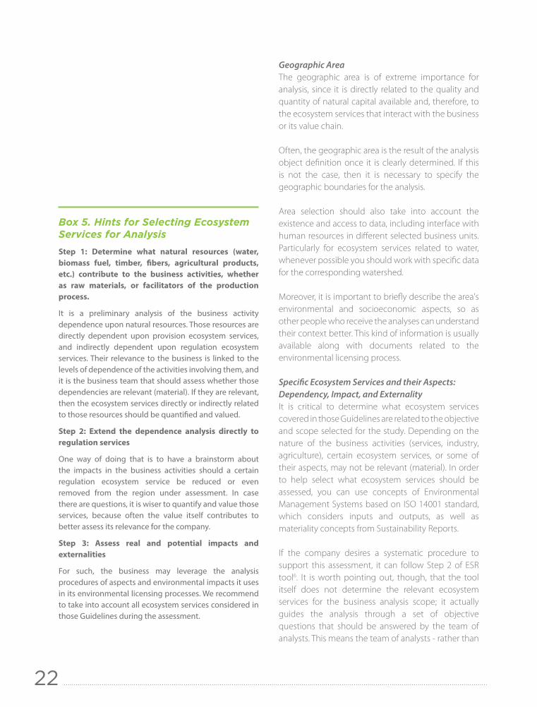
Box 5. Hints for Selecting Ecosystem Services for AnalysisStep 1: Determine what natural resources (water, biomass fuel, timber, fibers, agricultural products, etc.) contribute to the business activities, whether as raw materials, or facilitators of the production process.

It is a preliminary analysis of the business activity dependence upon natural resources. Those resources are directly dependent upon provision ecosystem services, and indirectly dependent upon regulation ecosystem services. Their relevance to the business is linked to the levels of dependence of the activities involving them, and it is the business team that should assess whether those dependencies are relevant (material). If they are relevant, then the ecosystem services directly or indirectly related to those resources should be quantified and valued.

Step 2: Extend the dependence analysis directly to regulation services

One way of doing that is to have a brainstorm about the impacts in the business activities should a certain regulation ecosystem service be reduced or even removed from the region under assessment. In case there are questions, it is wiser to quantify and value those services, because often the value itself contributes to better assess its relevance for the company.

Step 3: Assess real and potential impacts and externalities

For such, the business may leverage the analysis procedures of aspects and environmental impacts it uses in its environmental licensing processes. We recommend to take into account all ecosystem services considered in those Guidelines during the assessment.

23

the tool - makes the decision on the relevance of ecosystem services.

Lastly, it will be necessary to select what aspects of ecosystem services will be considered in the analysis: dependency, impacts that affect the business, and/or externalities. The relevance analysis of ecosystem services will indicate what aspects should be considered for each ecosystem service assessed. However, there will be cases in which the team of analysts will be responsible for assessing whether the impacts affect the business or are rather generated by it – the so-called externalities. When determining the aspects to be studied, it is important to also think of data availability.

Time Horizon and Intergenerational Discount RateTime horizon is the period considered in the analysis. When this is period is up to one year, as usual in retroactive inventory analysis, estimated values can be considered up to date, as long as the economic data that supported the analysis is also up to date (product prices, or cost of replacement services, or complementary services to the assessed ecosystem service obtained in the current year, for instance). Should the time horizon be longer than a year, it will be necessary to update the estimates for the other years according to their present value. This is common practice for project retroactive or prospective analyses.

The need to update future estimates according to present value poses one of the major challenges and controversial topics in environmental economic valuation, which is how to determine the intergenerational discount rate. This is the rate used to update past and future ecosystem service flows, expressed in monetary value, according to their present value, in order to consolidate the estimate for the entire time horizon established for the analysis. The expression 'intergenerational' refers to the impact the selected rate may have on the equity between

Box 6. Inventories as an Environmental Performance Monitoring ToolThe practice of regularly making inventories of dependencies, impacts and externalities may be used as a tool to monitor risks and performance. Here are some remarks to help elaborate a monitoring program based on physical or monetary ecosystem service metrics.

Determining the periodicity, that is, the frequency interval for measuring, is critical for monitoring effectiveness. Shorter periodicity implies greater effort and, therefore, higher costs, but it does not necessarily ensure more accurate data. Certain ecosystem services, due to their natural dynamics, take longer than others to reflect the impacts of actions derived from business decisions, and excessive short periodicity applied to this natural dynamics will not be more efficient in monitoring those impacts. Similarly, very long periodicity applied to the ecosystem service natural dynamics, although the costs for monitoring are lower, may fail to capture important information on its variation.

Usually, annual periodicity consists of a good option for corporate inventories, except for the comments previously made, since it is related to the fiscal year and is less likely to be influenced by seasons.

6 ESR = The Ecosystem Services Review, available at < www.wri.org/publication/corporate-ecosystem-services-review>

24

current and future generations when it comes to ecosystem service allocation and availability.

In short, the higher the discount rate applied, the lower the economic value assigned to the ecosystem service future flow. Thus, if the rationale used to choose the rate is solely financial, it may devaluate future natural capital and, therefore, the decision on the rate should take into account other factors, such as:

• Financial update of economic values of ecosystem service future flows applying a certain rate, necessarily based on financial market interest rates, assumes that ecosystem services can be replaced with financial capital, which does not reflect the reality

• Devaluation of ecosystem service future flows is likely to favor consumption and degradation of natural capital by current generations, compromising the provision of natural capital for future generations

• The environment has other critical factors that are not economic (sociocultural and ecological values), which can also be compromised should the discount rate privilege its devaluation and, consequently, its degradation

• Considering the Brazilian historical trend to lose natural capital in exchange for consumption or environmental degradation, the most plausible trend is that there will be fewer natural resources as ecosystem services; and the economic value of those that cannot be replaced, like water, should actually be higher, rather than lower, than the current value.

Interest rates applied in the international financial market are usually taken as reference to determine the discount rate. Nevertheless, there is no objective criterion that is widely and fully accepted to guide that decision. There are important subjective criteria to take into account, and the choice will necessarily be based on ethical considerations. The formula for financial update of future values associated to ecosystem services, typically used for cash flows, is available in Appendix 1.

Data AvailabilityPre-assessment of data availability is critical early in the planning stage. Data needed for analyses is indicated and determined in the method formulas presented for each ecosystem service.

For data that can be collected in-house, you need to determine whether it is available and who can provide it, or if it is necessary to produce it, and who will be in charge of it.

For data that cannot be collected in-house, you need to determine whether it is available and can be collected and/or produced externally, considering if economic valuation calculated with this data justifies the costs for obtaining it.

It is recommended to elaborate a checklist containing the data to be collected, people in charge of collecting it, the information source, and the desired technical parameters. For data gathered from different sources (suppliers, for instance), special care should be taken to have consistent units of measurement.

TeamTeams should be formed according to the need to collect and analyze data. It is critical to consistently analyze internal capacity, as well as time availability. If internal resources are not sufficient to meet the study demands, external help should be hired.

While forming teams, the following should be taken into account:

C-level ManagersEngaging one or more C-level managers in the business is critical to support the work planning and development. Participation of C-level managers is welcome while elaborating the analysis (its objective and scope); and it is essential to ensure formality of the analysis process and access to internal data in a timely manner to meet the planned schedule.

25

Work CoordinationIt is critical to assign a coordinator with proper authority to guide the team. Preferably, the coordinator should be familiar with the business operation and have some technical expertise on environmental economic valuation.

In summary, the coordinator's responsibilities include: a) ensure the work execution dynamics, stick to the schedule and objectives as determined in the work plan; b) request other areas to provide data (usually supported by C-level managers); c) coordinate internal analysts' work; d) hire and coordinate the work of eventual external analysts; and e) mobilize the engagement of suppliers/customers when analyses involve the value chain.

Internal AnalystsIn charge of verifying and sorting data, applying valuation methods, and generating results from analyses.

External TeamUsually works in coordination or analysis roles, whenever the internal team is not available to perform those functions.

BudgetIt is important to create a budget, so as to manage the necessary resources to execute the work. Here are some examples of activities whose costs should be considered: a) production of internal data; b) collection of external data; c) team building; d) travel time and trips; and e) hiring third-parties.

Schedule of ActivitiesIn order to support and facilitate the control of activities in the economic valuation process, it is recommended to build a detailed schedule, with different activities to be performed, their corresponding deadlines and people in charge of them, particularly when the estimate is being calculated for the first time.

METHODS FOR QUANTIFICATION AND ECONOMIC VALUATION OF ECOSYSTEM SERVICES

27

7 Refers to ecosystem integrity, health and resilience, or minimum conditions for them to keep providing ecosystem services (TEEB, 2012a).8 Aesthetic, spiritual, cultural inspiration, cognitive, social relationships, among others, depending on the author.

Below, you will find simplified methodological guidelines for quantification and economic valuation of dependencies, impacts that affect the business, and externalities related to 8 ecosystem services:

• Water provision (quantity)• Biomass fuel provision• Water quality regulation• Regulation of wastewater assimilation• Global climate regulation• Pollination regulation• Soil erosion regulation• Recreation and tourism

The typology adopted to sort ecosystem services is the one proposed by TEEB (2012a). Methodological guidelines were elaborated independently for each ecosystem service, so businesses can select and analyze only the ecosystem services that are relevant to the scope determined in the study.

Descriptions of ecosystem services are based on their theoretical definitions, but were adapted to better reflect the reality in business environmental management.

For determining methodological approaches, priority was given to simplified methods capable of producing realistic estimates from the economic perspective, and that were representative of the business world. For such, methodological procedures aligned with actions usually considered by businesses in prevention or remedy of environmental damages were privileged, thus contributing to a previous economic assessment of management action alternatives.

It is important to highlight that the methods indicated cannot estimate the total value of a natural resource (ecosystem service or good), only its economic value.

Business decision-making process, therefore, should not ignore other values associated with the environment, whether ecological values7, or different sociocultural values8. Lastly, sheer economic valuation, in spite of generating relevant information

for business, underestimates the real value of an ecosystem service or good, and should be understood from this perspective.

Assuming all dependencies are linked to risks, and when risks come true they translate into impacts that affect the business, the greater impact that will affect the company due to variation in ecosystem service availability will be equivalent to the level of dependence the business has upon it.

Methodological procedures for dependencies and impacts were aligned based on this rationale. As many of the variables used in the guidelines for both are the same, you will only find descriptions for the variables that were not previously described for dependency upon the same ecosystem service. However, in the guidelines for externalities, all variables are described, even the ones that are common to guidelines for dependencies and impacts, so readers will not have to go back in the text looking for those variable definitions.

All methodological procedures were described and illustrated in as much detail as possible and needed so the estimate process can be understood and assessed. The complexity of those procedures varies according to the ecological and economic assumptions that support them, but calculation can be performed in an Excel spreadsheet provided by TeSE; all you need to do is input data and, in some cases, choose some available criteria and analysis parameters.

All the methodological procedures described in this document can be implemented by using the DEVESE calculation tool, provided by TeSE for free (www.tendenciasemse.com.br).

28

Ecosystem Services

Dependency Impact Externality Important RemarksQuantification Valuation Quantification Valuation Quantification Valuation

1. Water provision (quantity)

Demanded water / Production

RCM Hydrological drought

RCM Hydrological balance in critical watersheds

RCM –

2. Biomass fuel provision

Biomass / Total demand of fuel

MPMe Quantity of most cost-effective energy alternative

RCM 1. Productivity of the removed economic activity

2. GHG emissions from fossil fuel alternatives

1. OCM2. RCM (SCC)

–

3. Water quality regulation

Desired quality / Worst quality known

RCM Quality obtained / desired quality

RCM Upstream quality / downstream quality

ACM Positive impacts or externalities are not determined

4. Regulation of wastewater assimilation

– – – – Pollutant load produces environmental changes

ACM Dependency equivalent to externality Impact was not determined

5. Global climate regulation

– – – – GHG biogenic removals and emissions Avoided deforestation

RCM (SCC) It is recommended to include emissions from other sources, calculated separately

6. Pollination regulation

Additional productivity as a result of bee pollination

1. RCM2. MPM

1. Effort to replace pollination

2. Variation in the supply of natural pollination

1. RCM2. MPM

Variation in the supply of natural pollination for third-parties

MPM –

7. Soil erosion regulation

1. Potential local loss of soil nutrients

2. Potential turbidity in collected water

RCM 1. Local loss of soil nutrients

2. Turbidity in collected water

RCM Turbidity in water upstream

RCM –

8. Recreation and tourism

– – 1. Visitation per period

2. Productivity of land use alternative

1. TCM (partial)2. OCM

Travel (including accommodation out of the visitation area)

TCM (partial)

No dependency was determined in this case

RCM = Replacement Cost Method; MPMe = Market Price Method; OCM = Opportunity Cost Method; ACM = Avoided Costs Method; SCC = Social Cost of Carbon; MPM = Marginal Productivity Method; TCM = Travel Cost Method

Table 1. Table summarizing quantification metrics and economic valuation methods adopted

29

WATER PROVISION

Refers to the amount of freshwater used by the company, without considering the quality of the water.

This topic covers dependency, impact on the business, and externality.

DependencyDependency, in this case, refers to the amount the business needs to meet the production supply, or to provide the services required.

Quantification:

Physical metric: DQw = Qwd /Qpmax

Where Qwd = Qwun + Qwu

Where: DQw = Dependency on the quantity of water

Qwd = Quantity of water demanded, in m3 9

Qwu = Quantity of water currently used, in m3

Qwun = Quantity of water demanded but currently unavailable, in m3

Qpmax = Maximum quantity produced, in the corresponding physical facility.

Basically, in order to calculate Qwd, it will be necessary to measure all the demanded water volume, both in the production process and in ancillary activities considered essential for the business operation. That amount of water includes both the water currently used, Qwu and the water that would be used if available Qwun.

9 1m3 = 1,000 liters

30

To calculate the volume of water currently used, Qwu, you can apply the Water Footprint10 methods. Included in the calculation of water that is actually used are the following: a) water that is directly collected (surface water, underground water, or rainwater), which corresponds to the blue footprint; b) water that is provided and charged by water supply companies; c) water needed for agricultural production, whenever applicable, which corresponds to the green footprint in the context of products' water footprint.

Specifically for water needed in agricultural production, whenever it is not possible to directly calculate the green footprint, you can use estimates published in specific studies11. Should there be no estimates for the product, you can use as reference the green footprint of a similar product.

When calculating Qwd, the following should be taken into account: a) water used during production, whether incorporated into the product or not; b) water lost (evaporation, leak, etc.); as well as, c) water indirectly used (to keep administrative or support activities, such as water used in toilets, kitchens and to clean administrative facilities), as long as it is vital for the business operation.

As for the volume of water that would be used if available, Qwun, can be obtained from the business operational area (Engineering), or estimated according to the growth expected in production with that additional volume of water. If using estimates, all you need to do is multiply the current volume of water actually used times 100%, plus the percentage of production growth expected with the use of that additional volume of water.

For Qpmax, you shall consider the maximum production of the business in its current structure, should all water needed be available. When calculating the

production indicator, the metric adopted shall be the one that best fits the business production; i.e.; units of measurement for volume or mass (m3, tons, liters, etc.) for industries; and number of collaborators for service providers. If the business manufactures more than one product, with different characteristics, it can separately calculate the dependency physical indicator, DQw, for each.

ValuationThe valuation method adopted is the Replacement Cost (Annex 1), used in this case to estimate the costs the business would need to pay to replace the amount of water it demands (therefore, upon which its production depends), but is not available.

Value of the dependency = Qwd x $pwimp + $logiw

Where: $pwimp = Price of imported water (from another watershed), in BRL/m3

$logiw = Cost of logistics to import the water, in BRL

To determine $pwimp, you directly contact the water supplier. For this assessment, you should consider water in proper condition for the business use, regardless of the amount of water that was being collected.

To determine $logiw you can also contact water supply companies, since they usually include delivery in their service portfolio, or, else, you may contact other delivery carriers. In case you need to make adjustments in your infrastructure to receive the water purchased, corresponding costs and any extra costs incurred should also be included in $logiw, in this context.

31

ImpactImpact, in this case, refers to consequences of water shortage for the business activities.

Quantification:

Physical metric: Hd = Qwun

Where: Hd = Hydrological drought that actually compromises levels of production, in m3

To determine Qwun you shall follow the same procedures described on the previous topic about dependency.

ValuationThe valuation method adopted is the replacement cost (Annex 1), used in this case to estimate the costs needed to replace the hydrological drought (Hd).

Value of the impact = Hd x $pwimp + $logiw

To determine $pwimp and $logiw, you shall follow the same procedures described on the previous topic about dependency.

ExternalityExternality, in this case, refers to consequences, to other users, produced by the shortage of water due to the collection and use by the company in watersheds whose hydrological availability has already been distributed to different users.

Quantification:

Physical metric: Hb = Qwcol - Qwret

Where: Hb = Hydrological balance of how much water the business uses, in m3

Qwcol = Quantity of water collected, in m3

Qwret = Quantity of water returned to the same body of water where it was collected, in m3.

Data on the current status of the watershed hydrological availability can be obtained from technical studies, such as maps of water stress, as well as reports from the Water National Agency (ANA) and water agencies linked to local or regional watershed committees (i.e.; Piracicaba, Capivari and Jundiaí Rivers Committee – PCJ, in Sao Paulo).

Return of the water used shall occur upstream the first user collection point, immediately downstream where the business collected the water, in order to ensure users, especially those living in the company's surroundings, are not affected by water shortage related to Qwcol, rather than Hb.

ValuationThe valuation method adopted is the Replacement Cost (Annex 1), which in this case estimates the costs of replacing the water used with imported water from another watershed that still has hydrological availability to assign. In fact, that approach values preventing externalities, rather than their real or potential costs, and it is more relevant in a strategic context for businesses willing to invest on prevention. In the 'Important Remarks' topic, below, methodological procedures are indicated to estimate real and potential costs of those externalities.

Value of the externality = Hb x $pwimp + $logiw

Where: Hb = Hydrological balance of how much water the business uses, in m3

$pwimp = Price of imported water, in BRL/m3

$logiw = Cost of logistics to import the water, in BRL.

10 The water footprint of a business or one of its facilities corresponds to all freshwater directly or indirectly used in their activities. Basically, it can be sorted into blue footprint, green footprint and gray footprint. For further information, please go to www.waterfootprint.org 11 There are studies for many products that you can access for free under the 'Product Water Footprints' link, at the following website: www.waterfootprint.org

32

Important RemarksTo calculate the water footprint, both blue and green, you shall account for the water use, rather than only consumption; meaning even water lost along the production process and water indirectly used should be accounted for.

The valuation method called Marginal Productivity Method (or dose-response function – Annex 2), MPM, allows for a more accurate valuation, since it is not sensitive to price variations in replacement or complementary goods or services, as in methods such as RCM and ACM, or Avoided Costs Method (Annex 3). However, MPM demands data that may be hard to get, and is based on a dose-response function that may be difficult to estimate.

When it comes to impact, in case it is not feasible to import water, the value of the impact will be equivalent to the value of what could not be produced due to the hydrological drought. Thus, it can be estimated by the cost of what could not be produced, in case you are not sure the production would actually be sold, or else you could estimate the revenue from the sale of the goods that could not be produced – in case the production has been sold in advance – or in case you are sure you would sell the products at the regular prices usually charged by the company.

Valuing externality real or potential costs often takes a long time, and is more expensive than the prevention approach, as indicated earlier. This happens because of the difficulty to get data that accurately represents damages incurred (or estimated). Lastly, to estimate externality real or potential costs, you shall first determine what players were (or would be) affected by the water shortage, and how each one was (or would be) affected by scarcity. With this data in hand, it is possible to proceed with the economic valuation, applying the Replacement Cost Method, RCM, or the Marginal Productivity Method, MPM. Using RCM, valuation will be based on the replacement of economic damages incurred by each water user. Using MPM, valuation will be based on an estimate of economic activity loss for affected users, which may have values that are different from replacement costs.

Box 7. Example: Water ProvisionAnglo American has a ferronickel industrial plant in Barro Alto, in the state of Goias, Brazil, that counted with US$ 1.9 billion in investments and was launched in December 2011. Throughout its life cycle, it will produce 36,000 t of nickel contained in ferronickel per year, on average. It is a strategic project, because it increases the business international ferronickel market share from 8% to 11%.

In the production process, water is used with the heat exchange function in the metal granulation, cooling of electric furnace, and magnesium silicate granulation (process waste) steps. All water used in those steps is reused in the circuit, therefore it is a zero-waste water operation, and the average recirculation rate is 85%. Thus, from all water that enters the circuit, about 2,000,000 m3 per month, 15% needs to be replaced due to losses caused by evaporation. On average, those 15% account for a volume of 300,000 m3, considering some variation between rainy seasons (from November to March) and dry seasons (from April to October).

DEPENDENCYThe plant uses a pyrometallurgical process and relies on two high-power electric furnaces for ore reduction; cooling the furnace housing is dependent on heat exchanges with water; besides, smelted material (metal smelted at 1,500 °C / 2,732 °F) also depends on water to granulate and solidify. Therefore, water is an essential element in this process.

Quantification

Year 1: DQw = Qwd /Qpmax = (2,000,000 + 300,000 x 11)/36,000 = 147.22 m3/t

Other years: DQw = Qwd /Qpmax = (300,000 x 12)/36,000 = 100 m3/t

The supplier who could eventually supply Barro Alto plant in case of lack of water in the region would be Goias state water supplier (SANEAGO), which currently charges BRL 5.98/m3. Barro Alto plant is located far from urban areas, so it cannot be reached by SANEAGO current network. The closest village where the network is connected to is about 50 km (31 miles) away, and costs for extending the network would definitely have to be paid by the business. To build its current collection system in Barro Alto, Anglo American had to invest about BRL 250,000.00/km in order

33

to install pipes, besides having to pay compensation to landowners in the places where the pipes were installed. Nonetheless, given a scenario of scarcity that justifies such a large investment, rural landowners living where SANEAGO pipes were installed would also probably feel the consequences of lack of water and, therefore, we assume they would not demand any compensation for having the pipes installed in their lands, since they would also benefit from this new source of water.

Value of the dependency

Year 1 = Qwd x $pwimp + $logiw = (2,000,000 + 300,000 x 11) x 5.98 + (50 x 250,000) = BRL 44,194,000.00

In year 1, in the first month, they would need 2,000,000 m3 of water to keep the production levels, whereas in the other years they would only need to replace the 15% lost due to evaporation. Moreover, in this year they would amortize the costs incurred in extending the water network.

Other years = Qwd x $pwimp + $logiw = (300,000 x 12) x 5.98 = BRL 21,528,000.00

In the other years, they would only need to replace the water lost due to evaporation.

Comparing future values projected for the next 10 years updating them with a 5% interest rate per year, equivalent to TJLP12 rate in 2014, you get:

Value in 10 years, with no discount = BRL 215,280,000.00Value in 10 years, discounted = BRL 166,233,509.56

In short, financial update for 10 years depreciated the water provision value in 23%. Similar depreciation is applied to impacts and externalities, if you keep the same rate and time period.

IMPACTImpact, in this case, was simulated assuming partial and permanent reduction in water availability in the current source of water collection, whose maximum volume to be collected will be 200,000 m3/month.

Quantification

Hd = Qwun = Qwd - Qwu = 300,000 m3/month - 200,000 m3/month = 100,000 m3/month

Value of the impact

Year 1 = Hd x $pwi + $logiw = (100,000 x 12) x 5.98 + (50 x 250,000) = BRL 19,676,000.00

Other years = Hd x $pwi + $logiw = (100,000 x 12) x 5.98 = BRL 7,176,000.00

EXTERNALITYAssuming the hypothetical scenario in which the watershed where the business collects water is fully allocated to other users, if the business used the water it would cause shortage of water downstream the watershed and, consequently, an externality, particularly if downstream use were priority compared to industrial use, as in the case of public supply and drinking water for livestock.

Quantification

Physical metric:

Year 1: Hb = Qwcol - Qwret = (2,000,000 + 30.000 x 11) - 0 = 5,300,000 m3

Other years: Hb = Qwcol - Qwret = (30.000 x 12) - 0 = 3,600,000 m3

Value of the externality

Year 1: Hb x $pwi + $logiw = 5,300,000 x 5.98 + (50 x 250,000.00) = BRL 44,194,000.00

Other years: Hb x $pwi + $logiw = 3,600,000 x 5.98 = BRL 21,528,000.00

This example was elaborated for learning purposes, using data provided by Anglo American.

12 TJLP = Long-term interest rate adopted by BNDES, the Brazilian National Bank of Social and Economic Development

34

BIOMASS FUEL PROVISION

Refers to all plant or animal derived matter used as fuel. In those guidelines, we consider only plant-based biomass. For this ecosystem service, we assess dependency, impacts that affect the business, and externalities.

DependencyDependency, in this case, refers to the amount of biomass fuel needed for the business activities.

Quantification:

Physical metric: DBf = Qb / tQf

Where Qb = Qbu + Qbr

Where: DBf = Dependency on biomass fuel, in percentage

Qb = Quantity of biomass needed for business activities (m3, tons, liters, etc.)

tQf = Total quantity of fuel needed for business activities (m3, tons, liters, etc.)

Qbu = Quantity of currently used biomass (m3, tons, liters, etc.)

Qbr = Quantity of biomass to be replaced due to unavailability in the period (m3, tons, liters, etc.).

ValuationThe valuation method adopted is the market price13 method, which in this case directly uses biomass fuel market price as an estimate of its economic value for the business.

13 In this case, we used for value estimate the biomass market price. It is worth pointing out that market price is not always a good economic value gauge, since it is subject to market distortions, such as information asymmetry, difficulty of some people to access the market, particularly low income population, etc.

35

Value of the dependency = Qb x Mpb

Where: Mpb = Market price of biomass, in BRL

ImpactThe impact of using biomass fuel in business activities can be measured by the amount of the most cost-effective alternative energy source for the company that would be necessary to replace the biomass that is currently unavailable (Qbr), or else the biomass that was being used, but was lost.

Quantification:

Physical metric: IBf = Qealt= Qbr x Efcp

Where: IBf = Impact of loss (or lack) of biomass fuel

Qealt = Quantity of the most cost-effective energy alternative, in its corresponding units (m3, kW, MW, tons, liters, etc.)

Efcp = Equivalence factor of calorific potential to adjust the quantity of the alternate energy source so it generates the same calorific potential as the biomass.

The quantity of the most cost-effective energy alternative , Qealt, shall be equivalent to the amount of biomass demanded that was never available, or equivalent to the biomass that was being used, but was lost somehow, such as in drop in production (Qbr). The calorific potential equivalence factor, Efcp, can be obtained directly from secondary data, or deducted from individual biomass calorific values (Cpb) and from the alternate source (Cpalt), as follows: Efcp = Cpb / Cpalt, paying special attention to the conversion of units between both energy sources.

ValuationThe valuation method adopted is the Replacement Cost Method (Annex 1), which, in this case, directly uses market prices for biomass fuel and its most cost-effective energy alternative as reference to estimate the monetary value of using biomass.

Value of the impact = Qealt x Mpalt - Qbr x Mpb

Where: Mpalt = Market price for most cost-effective energy alternative, in BRL

ExternalitiesExternalities, in this case, are analyzed under two perspectives: a) land use change as a consequence of biomass production; b) avoided GHG emissions due to the use of fossil fuels, in case some fossil fuel happens to be the most cost-effective energy alternative for the business.

In the first case, externalities are land use changes that remove economic activities that are currently generating benefits for other stakeholders, particularly food production. Only land use changes as a direct consequence of the business demand for biomass shall be considered.

In the second case, whenever the most cost-effective energy alternative for the business is some kind of fossil fuel, you shall estimate their corresponding GHG emissions. As the use of biomass implies avoided emissions of the fossil alternative, it is considered positive externality.

Quantification:

Physical metric 1: EBfluc = Pear x A

Where: EBfluc = Externality associated with land use change to favor biomass fuel production

Pear = Average annual productivity of the economic activity that was removed, per area unit

A = Area of the economic activity removed

36

EBfluc estimates shall consider all areas whose economic activity was replaced with biomass production purchased by the business. For instance: if biomass production purchased by the business replaced milk production in a 10 ha area whose productivity was 100 liters/ha x year, then Pear = 100 l/ha x 10 ha = 1000 l/year.

Physical metric 2: EBffa = Qfalt x EFfalt

Where: EBffa = Externality due to avoided GHG emissions from the most cost-effective energy alternative for the business if this alternative is fossil fuel, in tCO2e

Qfalt = Quantity of fossil fuel alternative that would be necessary to replace biomass used by the business, in units such as m3, liters, or tons

EFfalt= Emission factor of the most cost-effective fossil energy alternative for the business

To calculate EBffa, you can use Brazil GHG Protocol Program calculation tool, free of charge, available on the Internet14.

ValuationThe valuation method adopted for metric 1 is the opportunity cost method (Annex 4)15, which estimates the monetary value of the economic activity removed in order to produce biomass.

The valuation method adopted for metric 2 is the Replacement Cost Method (Annex 1), used here to estimate expenses that in theory would be necessary to compensate eventual climate change adverse impacts on society, if biomass fuel consumed by the business were replaced with fossil fuels16.

Total value of externalities = VEBf1 + VEBf2

Where: VEBf1 = EBfluc x Mpear

VEBf2 = EBffa x SSC

Where: Mpear = Product or service market price of the economic activity removed due to expansion of biomass fuel production, in BRL

SCC = Social Cost of Carbon, in BRL

The SCC value adopted in this guide is US$ 38.00, as calculated by the U.S. government (you will find further details in Annex 5), and it shall be converted into Brazilian Reals according to the official American dollar exchange rate published by the Brazilian government 17.

Important RemarksResidues from agricultural or forestry production do not generate land use change; therefore, they shall not be considered in VEBf1 or Pear.

Land use changes due to biomass production involving deforestation, even though they are not replacing an economic activity, also produce externalities. But, as this type of externality is measured and valuated in the climate regulation analysis, it was not repeated here to avoid double counting. This includes both timber and forestry residues.

Quantification and valuation of the externality characterized by GHG emissions from use of biomass are also estimated in the guidelines for climate regulation ecosystem service, and that's why they were not developed again for this ecosystem service. In case the business judges this information relevant to analyze biomass, it can use the climate regulation guidelines to get it.

14 Brazil GHG Protocol Program website: www.ghgprotocolbrasil.com.br15 Opportunity cost is defined (by DAILY & FARLEY, 2010) as the 'best alternative you forgo when you make a decision'.16 Therefore, it is the same method adopted for Global Climate Regulation ecosystem service.17 Exchange rates, the Brazilian Central Bank: www.bcb.gov.br/?txcambio

37

18 Converting 300 t into kg, because the calorific potential was calculated based on kg of firewood

Box 8. Example: Biomass Fuel ProvisionA food processing business uses 1,500 t of eucalyptus reforestation firewood per year to fuel its boilers. Its facilities, however, have capacity to increase production, but it would require a 20% increase in power consumption should local suppliers be able to increase their firewood production.

DEPENDENCYThe industrial plant does not operate without the energy produced in the boilers, so production is fully dependent on firewood supply.

Quantification

DBf = Qb/tQf = (Qbu + Qbr)/tQf = (1,500 + 300)/1,800 = 100%

Firewood price was quoted at BRL 500.00/t, freight included.

Value of dependency = Qb x Mpb = 1,800 x 500.00 = BRL 900,000.00

IMPACTThere are no power transmission lines in the industrial plant surroundings, and the most cost-effective alternative to replace unavailable biomass Qbr is diesel oil.

Quantification Considering the calorific potential of one kilo of firewood is approximately 50% of the calorific potential of one liter of diesel oil, in order to replace 300 t of reforestation firewood that are currently unavailable, about 150,000 l of diesel oil will be required.

IBf = Qealt = Qbr18 x Efcp

= 300,000 x 50% = 150,000 l of diesel oil

Diesel oil price was quoted at BRL 2.40/l, freight included.

Value of the impact = Qealt x Mpalt - Qbr x Mpb = 150,000 x 2.40 - 300 x 500.00 = BRL 360,000.00 - BRL 150,000.00 = BRL 210,000.00

EXTERNALITIESTwo types of externalities can be characterized in this case: a) replacement of family farming areas with production of reforestation firewood; b) avoided emissions thanks to replacement of diesel oil with biomass to fuel the boilers.

QuantificationAverage productivity of eucalyptus forests in the region is 50 m3/ha per year, the equivalent to about 700 kg of firewood/ha. Thus, to supply the annual demand of 1,500 t of firewood, they need about 2,200 ha of forests to produce firewood. From this total, at least 200 ha replaced areas that used to be subsistence dairy farms (1 animal/ha), whose productivity was 1,500 l/ha x year.

(1) EBfluc = Pear x A = 1,500 x 200 = 300,000 l of milk per year

(2) EBffa = Qaltf x EFaltf = 150,000 x 2.631 = 394,500 kgCO2e = 394.5 tCO2e

The price of one liter of milk was quoted at BRL 1.15 in the region.

Value of the = EBfluc x Mpear + EBffa x SCC externalities = 300,000 x 1.15 + 394.5 x (38.00 x 2.50) = BRL 382,477.50

Exchange rate used: BRL 2.50/US$

1 Factor only for CO2.

2 Estimated using Brazil GHG Protocol Program calculation tool based on factors known for commercial diesel (commercial diesel is not pure) and also considering factors for CH4 and N2O.

This is a fictitious example, elaborated for learning purposes, and the values used were estimated after consulting technical documents available on the Internet.

38

WATER QUALITY REGULATION

It refers to the quality of the water needed for business activities, considering its three fundamental aspects:

• Physical: Suspended solids, temperature19, etc.• Chemical: Existence and concentration of substances

from industrial processes wastewater, crop protection and agricultural fertilizers, household sewage, etc.

• Biological: Existence of microorganisms, particularly pathogenic microorganisms

This topic covers dependency, impact on the business, and externality. Illustrations of the dependency and impact concepts as adopted in this document can be seen in Appendix 2. The concept of externality is easily understood from the concept of impact.

DependencyRefers to ecosystem contribution to the quality of the water used by the business. For instance: prevent erosion that increases the amount of suspended solids in surface water, regulate the water temperature, decompose household sewage and fertilizers, and biologically control pathogenic microorganisms.

The difference between the water quality resulting from almost total reduction or lack of ecosystem services – minimum quality – and the water quality the business needs to keep its operation (up to the quality limit the ecosystem is able to supply) – ideal quality – will represent the dependence the business has upon this ecosystem service.

19 Ecosystems are capable of regulating temperature, thus avoiding great thermal variations. In this sense, water with high temperatures (like the water used in cooling systems) released in the environment with potential to adversely impact local biological activity is more likely to have its heat dissipated faster by well preserved ecosystems, thus reducing damages caused to local biota.

39

Quantification:

Physical metric: DQlw = Qlwmin - Qlwideal

Where: DQlw = Business dependence upon the Water Quality Regulation Ecosystem Service

Qlwmin = Minimum water quality on its pick-up point, using the unit of measurement of the parameter being assessed, under minimum levels of ecosystem regulation, in highly degraded systems

Qlwideal = Ideal quality of water needed for business operation, using the unit of measurement of the parameter being assessed, on its pick-up point.

Quantification of DQlw shall be individually performed for each physical, chemical and biological parameter the business judges important.

In case of parameters proportionally related to water quality – i.e.; the higher their estimated value, the better the water quality – , their estimates or measurements shall be multiplied by -1.

If accurate data is not available, you can apply to Qlwmin the worst level ever observed (registered) in the body of water for the corresponding parameter. However, such reference may not actually represent the worst possible level of water quality in the region assessed.

A good alternative to estimate Qlwmin is to use hydrological models simulating the absence or low levels of the ecosystem service provision, such as in areas where the soil is exposed (no vegetation cover), for instance. Vegetation cover protects the soil from erosion, thus reducing the amount of suspended solids that make the water of rivers and other water springs look turbid. Specifically for suspended solids, Qlwmin can be estimated using the model represented by the universal soil loss equation (BERTONI & LOMBARDI NETO, 2008) and a sediment deposition rate into the body of water (please refer to guidelines for soil erosion regulation ecosystem service). InVEST20 model is a good alternative to get Qlwmin estimates for

different water quality parameters. Ideally, you should have specific data for that watershed, but, if there is not specific data, you can use estimates based on studies conducted in other watersheds with similar characteristics.

You can obtain Qlwideal with the water quality parameters needed for business operation, as specified by the business. If the company does not have its own parameters, it should use as reference standards and some classes determined by the Brazilian legislation, particularly CONAMA resolution #357/200521. Standards expected in CONAMA 357/2005 special class will represent the maximum levels of Qlwideal, since there is a limit to the water quality that can be provided by natural ecosystems. Superior water quality will have to be produced through specific technological processes; as they are not ecosystem services, they should not be considered in this analysis, though.

ValuationThe valuation method adopted is the Replacement Cost Method (Annex 1), which, in this case, estimates the expenses that would be necessary to recover the degraded water quality should no water quality regulation ecosystem service be available.

Value of the dependency = Qwcol x $Tw + Iwtp

Where: Qwcol = Quantity of water collected, in m3

$Tw = Cost to treat water from quality level Qlwmin to quality level Qlwideal, in BRL/m3

Iwtp = Investment needed in water treatment plant, in BRL

Qwcol variable shall be obtained from measurements performed by the business operational area. $Tw and Iwtp can also be obtained with the business operational area, or quoted in the water treatment service market. Investments on WTP can be amortized following traditional accounting criteria.

20 InVEST: www.naturalcapitalproject.org/InVEST.html21 CONAMA Resolution # 357/2005: www.mma.gov.br/port/conama/legiabre.cfm?codlegi=459

40

This dependency valuation method is also applied to businesses that buy treated water, since water treatment from quality level Qlwmin to quality level Qlwideal is mandatory, regardless if it is performed by the company itself or by another company whose business is to sell treated water. Costs may vary according to adoption of different operation technologies and scales, but the method rationale applies to both situations. If the water is purchased, all you need to do is replace the $Tw + Iwtp component from the above formula with the price paid for the water.

ImpactRefers to consequences of degradation in the quality of the water collected by the business, resulting in losses or damages to production, or the need for mitigation and compensation actions. In that sense, we consider the ideal water quality for the business that could be collected (quality as a result of ecosystem services conservation) and the real or actually observed quality of the water that has been collected.

Whereas for dependency, as described above, we assess the difference between the ideal quality and the worst possible quality where the water is collected, for impact we assess the difference between the ideal quality and the actual (real) quality where the water is collected.

Quantification:

Physical metric: IQlw = Qlwcol - Qlwideal

Where: w IQlw = Impact of lack or limitation of ecosystem services on quality regulation of water collected by the business

Qlwcol = Quality of water collected by the business

Qlwideal = Ideal quality needed for business operation, where water is collected.

If IQlw shows positive impact, it should be disregarded, since businesses cannot benefit from water with higher quality than actually needed.

Qlwcol shall be determined through laboratory analysis, either conducted by an in-house expert team at the business facilities, or hired from specialized labs. All water quality parameters relevant to business activities should be assessed.

For businesses that purchase treated water, but are still willing to estimate IQlw, they can choose the closest body of water more likely to have a license issued, and use it as reference for collecting water and determining Qlwcol. Qlwideal has been previously discussed, in the context of dependency.

ValuationThe valuation method adopted is the Replacement Cost Method (Annex 1), which, in this case, estimates the expenses that would be necessary compensate degraded water quality due to loss or reduction in water quality ecosystem regulation.

Value of the impact = Qwcol x $Tw + Iwtp


$Tw = Cost to treat water from quality level Qlwcol to quality level Qlwideal, in BRL/m3

Iwtp = Investment actually made on water treatment plant, in BRL

$Tw and Iwtp variables have been previously discussed in the context of dependency valuation.

Should the business purchase treated water, the value of the impact will be equivalent to the expenses to purchase water.

41

ExternalitiesRefer to consequences that affect other water users, with no proper compensation, derived from business activities on water quality ecosystem regulation.

Wastewater releases shall not be considered for the purpose of this analysis. They are an integral part of the 'wastewater assimilation' ecosystem service guidelines. We assume pollutants generated by business activities may exceed local ecosystem's ability to naturally assimilate and degrade them. You should consider here diffuse pollution sources, such as soil erosion and agrochemicals.

Quantification:

Physical metric: EQlw = Qlwu - Qlwd

Where: EQlw = Externality, or impact of business activities on the quality of water utilized by users other than the business itself

Qlwu = Quality of water upstream business activities

Qlwd = Quality of water downstream business activities

Qlwu and Qlwd shall be determined through laboratory analysis, either conducted by an in-house expert team at the business facilities, or hired from specialized labs.

All water quality parameters relevant to different land uses downstream business activities should be assessed. If there is no information on what those parameters are, you should analyze all parameters listed in official applicable water quality norms for the region, or CONAMA 357/2005.

ValuationThe valuation method adopted is the Avoided Costs Method (or Defensive Expenditure Method – Annex 3), which, in this case, estimates expenses needed to prevent degradation in water quality due to diffuse pollution sources under the business' responsibility.

However, this approach does not value real or potential costs of the externality in case it actually occurs, and it is more strategic for businesses willing to invest on

prevention. In the 'Important Remarks' topic, below, methodological procedures are indicated to estimate real and potential costs of those externalities.

Value of the externality = $EPdp

Where: $EPdp = Expenditures in actions needed to control or eliminate diffuse pollution sources resulting from business activities or activities in areas controlled by business

There are a number of actions needed to curb sources of diffuse pollution, and they vary according to the nature of those sources. However, all those actions can be quoted with environmental, conservation, and soil remedy consultancy firms.

Here are examples of actions to curb diffuse pollution sources: revegetation of soil erosion high risk areas, no-till farming to replace tillage in agriculture, replacement of nitrogen-based fertilizers with green manure, investments on biological control to reduce the use of crop protection, sewage plumbing and treatment, etc.

Important RemarksBy observing the characteristics of water quality degradation between upstream and downstream business activities, it is possible to check the types of diffuse pollution that have been affecting the body of water, which will help determine the strategies to reduce externalities.

As for Qlwd, you should be careful not to include wastewater impacts in your measurements. You can do that either by collecting water samples right before wastewater is released, whenever the release point is located downstream the business activities, or subtracting the wastewater polluting load from the polluting load found in the sample in order to determine Qlwd, which should not be hard to do, if there is control over wastewater polluting load released.

42

Valuing externality real or potential costs often takes a long time, and is more expensive than the prevention approach. This happens because of the difficulty to get data that represents damages incurred (estimated) in a realistic way. To estimate externality real or potential costs, you shall first determine what players were (or would be) affected by water quality degradation, and how each one was (or would be) affected. With this data in hand, it is possible to proceed with the economic valuation, applying the Replacement Cost Method (RCM, Annex 1), to remedy damages caused to each water user, or applying the Marginal Productivity Method (MPM, Annex 2), thus valuing loss of productivity in the water-dependent economic activity those users used to perform. Whenever possible, MPM method should prevail – since it uses specific data concerning the affected good or service, so it is less subject to distortions when compared to RCM, which is dependent on replacement services and goods markets.

Investments on WTP can be amortized following traditional accounting criteria.

Box 9. Example: Water Quality RegulationA food business uses 10.000 m3 of water/year both in its production process and for cleaning its facilities. The water used in the production process is not actually incorporated into the product; however, in order not to damage the product quality, the accepted level of suspended solids cannot be greater than 40 UNT (Nephelometric Turbidity Units), the equivalent to Class 1 freshwater, according to CONAMA Resolution 357/2005.

DEPENDENCYA hydrological model applied to the watershed where the business collects water indicates that, considering local soil and relief characteristics, absence of native vegetation in riparian areas and slope protection would imply increase in turbidity to approximately 350 UNT in the place where the business collects water.

Quantification

DQlw = Qlwmin - Qlwideal = 350 - 40 = 310 UNT

Approximate cost for water turbidity treatment is BRL 0.1233/m3. WTP infrastructure was estimated to be BRL 300,000.00, and labor costs for operation BRL 120,000.00/year.


Year 1 = Qwcol x $Tw + Iwtp = 10,000 x 0.1233 + (300,000 + 120,000) = BRL 421,233.00

The business would choose to amortize all WTP installation costs in the first year, since those costs would be fully incorporated into the financial statements corresponding to this year.

Other years = Qwcol x $Tw + Iwtp = 10,000 x 0.1233 + 120,000 = BRL 121,233.00



43

Value in 10 years, with no discount = BRL 1,212,330.00

Value in 10 years, discounted = BRL 936,129.09

In short, financial update for 10 years depreciated the water quality regulation value in 23%. Similar depreciation is applied to impacts and externalities, if you keep the same rate and time period.

IMPACTThe watershed from where the business collects water has been losing native vegetation cover in the past years, and current levels of water turbidity vary around 120 UNT.

Quantification

IQlw = Qlwcol - Qlwideal = 120 - 40 = 80 UNT

Approximate cost for treatment of water turbidity is BRL 0.1003/m3 and WTP infrastructure is the same estimated in case of dependency.

Value of the impact

Year 1 = Qwcol x $Tw + Iwtp = 10,000 x 0.1003 + (300,000 + 120,000) = BRL 421,003.00

Other years = Qwcol x $Tw + Iwtp = 10,000 x 0.1003 + 120,000 = BRL 121,003.00

EXTERNALITYThe business owns 50 ha of areas that are not used in its productive activities, but that were previously deforested and are experiencing erosion processes. Estimation for downstream turbidity was 180 UNT. Estimates for restoring those areas - which would reduce erosion processes and contribute to retain sediments from erosion - were of BRL 20,000,00/ha, including maintenance costs for two years.

Quantification

EQlw = Qlwu - Qlwd = 120 - 180 = - 60 UNT

Value of the externality = $EPdp = 50 x 20,000.00 = BRL 1,000,000.00

This is a fictitious example, elaborated for learning purposes, and the values used were estimated after

checking consultancy firms specialized in environmental sanitation and technical documents available on the Internet.

Costs for turbidity treatment were obtained from Constantino and Yamamura (2009) and updated according to IPCA index (projected in 6.50% for 2013).

44

REGULATION OF WASTEWATER ASSIMILATION

Refers to ecosystems' ability to dilute, assimilate and decompose wastewater in such a way as not to significantly change the water quality downstream the spot it is released.

Business dependency on this ecosystem service is estimated by ecosystems' ability to mitigate or even neutralize the damages wastewater released by the business may cause. Therefore, the value of this dependency corresponds to the value of the negative externality caused by the company that released it, because, in this situation, other social players, located downstream the spot where wastewater is released, will be affected by the environmental degradation caused by the business wastewater.

The business itself is not directly affected by the wastewater, so there are no impacts to assess (in case the business gets affected by its own wastewater, such impact will be captured by water quality regulation ecosystem service guidelines).

So, guidelines for quantification and valuation of this ecosystem service were directed to negative

externalities. This focus on externality, rather than on dependency, aims at placing the analysis closer to management actions targeted at preventing damages to social players located downstream the spot where the business releases its wastewater.

ExternalityRefers to degradation in quality of bodies of water located downstream the place where the business releases wastewater due to their polluting load, thus affecting the quality of water available to other social players.

Quantification:

Physical metric: WWe = Cpmax - Cp

Where: WWe = Wastewater externality concerning the parameter analyzed

Cpmax = Maximum concentration of the parameter in the body of water per m3 of water, ensuring there will be no significant change in the water quality

Cp = Concentration of the parameter per m3 of gross (non treated) wastewater, in the same unit used in Cpmax

45

WWe quantification shall be calculated for each parameter (pollutant) identified in wastewater released by the business.

Cp shall be determined through laboratory analysis, either conducted by an expert team at the business facilities, or hired from specialized labs.

Cpmax can be obtained along with water quality norms and standards with jurisdiction in the area where the body of water is located, considering standards determined by the legislation as the least restrictive limits to be accepted as reference in the analysis.

ValuationThe valuation method adopted is the Avoided Costs Method (or Defensive Expenditure Method – Annex 3), which, in this case, estimates expenses needed to prevent degradation in water quality in the spot where wastewater is released.

Nonetheless, this approach does not valuate real or potential costs of the negative externality, should it actually occur. The approach adopted by those guidelines is relevant in a strategic context for businesses willing to invest on prevention. In the 'Important Remarks' topic, below, methodological procedures are indicated to estimate real and potential costs of those externalities.

Value of the externality = Qwwrel x $Tww + Istp

Where: Qwwrel = Quantity of wastewater released, in m3

$Tww = Cost to treat wastewater from quality level Cp to quality level Cpmax, in BRL/m3

Istp = Investment needed to install and operate a sewage treatment plant capable of meeting the expected quality standards in Cpmax, in BRL.

$Tww and Istp variables can be obtained with the business operational area, or quoted in the wastewater treatment service market. Qwwrel shall be obtained from measurements performed by the business operational area.

Important RemarksIf Cp < Cpmax, there will be no need for wastewater treatment; $Tww and Istp will be = 0 and, therefore, Qwwrel = 0, meaning there is no externality.

Valuing externality real or potential costs is often more expensive and takes longer than the prevention approach. This happens because of the difficulty to get data that represents damages incurred (estimated) in a realistic way. To estimate externality real or potential costs, you shall first determine what players were (or would be) affected by water quality degradation, and how each one was (or would be) affected. With this data in hand, it is possible to proceed with the economic valuation, applying the Replacement Cost Method (RCM, Annex 1), to remedy damages caused to each water user, or applying the Marginal Productivity Method (MPM, Annex 2), thus valuing loss of productivity in the water-dependent economic activity those users used to perform. Whenever possible, MPM method should prevail – since it uses specific data concerning the affected good or service, so it is less subject to distortions when compared to RCM, which is dependent on replacement services and goods markets.

As for investments in STP-related physical and technological capital, they can be amortized according to traditional accounting criteria.

46

Box 10 – Example: Wastewater AssimilationA certain industry produces 240,00 t of paper per year. The industrial process heavily relies on water consumption, generating about 100 m3 of wastewater per ton of paper produced. The wastewater, characterized by the presence of chlorine in average concentration of 0.74 mg/l Cl, is discarded in a river nearby, whose water meets CONAMA 357/2005 Resolution Class I standard of 0.01 mg/l Cl.

EXTERNALITYIn order to prevent environmental and socioeconomic impacts downstream its facilities, the business is committed to treat its wastewater until it can be assimilated by the river ecosystem, thus ensuring the quality of the water to downstream users.

Quantification

WWe = Cpmax - Cp = 0.01 - 0.74 = - 0.73 mg/l Cl

Approximate costs for treating wastewater are BRL 0.20/m3; STP infrastructure was estimated in BRL 500,000.00 and labor costs for operating it were estimated in BRL 240,000.00/year.


Year 1 = Qwwrel x $Tww + Istp = (240,000 x 100) x 0.20 + 740,000 = BRL 5,540,000.00

Other years = Qwwrel x $Tww + Istp = (240,000 x 100) x 0.20 + 240,000 = BRL 5,040,000.00


Value in 10 years, with no discount = BRL 50,400,000.00

Value in 10 years, discounted = BRL 38,917,544.04

In short, financial update for 10 years depreciated the wastewater assimilation regulation value in 23%.

This is a fictitious example, elaborated for learning purposes, and the values used were estimated after checking consultancy firms specialized in environmental sanitation and technical documents available on the Internet.


47

GLOBAL CLIMATE REGULATION

Climate regulation ecosystem service has been key in the context of climate change. Global warming is inherently linked to increases in GHG concentration, particularly CO2, and ecosystems play a critical role in regulating the concentration of that gas.

Climate regulation through ecosystem services is mostly related to: a) the ability ecosystems have to remove atmospheric carbon dioxide (CO2) and fix it into biomass (Removal Balance, Rb, and Emissions Balance, Eb); and, b) maintenance of carbon stocks already fixed into biomass (avoided deforestation), thus avoiding new CO2, and, eventually, methane (CH4) emissions. Biomass burning and decomposition can be called biogenic emissions.

There are no methodological guidelines determined for dependencies or impacts for that ecosystem service, because there are no models able to locally or robustly estimate potential local impacts of climate change yet. It is widely known such impacts can be acute, as in extreme events such as droughts and floods, or chronic, such as continuous and permanent temperature rise. However, due to the diversity of environmental, social and economic conditions businesses operate, it was not possible yet to more accurately map those potential impacts.

So, externalities become focus of quantification and valuation for this ecosystem service. Externalities, on their turn, were subdivided into net emissions and avoided deforestation.

48

ExternalitiesNet Emissions Externalities are considered here whenever business operation directly or indirectly produces: a) removal with decomposition or burning of biomass in less than 30 years24; or b) formation of permanent biomass, meaning it is not subject to future removal and decomposition as a consequence of anthropic actions – including both biomass fixed from recovery of natural ecosystems that will be preserved, and biomass fixed by production forests where timber is used to manufacture durable goods that will last for at least 30 years.

Business activities that imply biomass decomposition or burning, as well as other sources of GHG emissions, account for negative externalities, whereas permanent biomass formation accounts for positive externalities.

Quantification:

Physical metric: BCO2e = RCO2 - ECO2

Where: RCO2 = CrecV x Arec

ECO2 = CremV x Arem

Where: BCO2e = GHG removal and emission balance, in tCO2e

RCO2 = CO2 permanent removal, in tCO2e

ECO2 = Emissions related to loss of

biomass, in tCO2e CrecV = Carbon stock contained in

recovered vegetation biomass; may include carbon above or below the ground, in tCO2e/ha

CremV = Carbon stock contained in removed vegetation biomass; may include carbon above or below the ground, in tCO2e/ha

Arec= Area where vegetation recovery occurred, in ha

Arem= Area where vegetation removal occurred, in ha

RCO2 may occur mostly in two ways: recovery of natural

ecosystems, or production of commercial forests. In both cases, permanent biomass is mainly associated with long life cycle woody species, such as trees and some types of shrubs.

To calculate ECO2, any type of vegetation removal

should be considered, discounting biomass removed and used for manufacturing durable goods25, assuming that biomass will not be converted into CO2 in the next 30 years.

Factors for CrecV and CremV per type of vegetation (phytophysiognomy) can be obtained from the 2nd Brazilian National Inventory of Anthropogenic GHG Emission and Removal (FUNCATE - Foundation of Spacial Science, Applications and Technologies, 2010), and are also available in DEVESE calculation tool. This kind of information can also be obtained from forest inventories, preferably in the regions selected in the valuation study.

Special attention should be paid to the units of measurement used for CrecV and CremV. The Brazilian national inventory, for instance, publishes such factors using tC/ha as the unit of measurement, and many forest inventories do the same. To convert this unit of measurement into tCO2e/ha, as used in the physical metric formula, shown previously, all you need to do is multiply it by 44/12.

The national inventory also offers factors to adjust tC/ha of a certain type of vegetation according to its successional stage, i.e.; factors to convert primary forest tC/ha into the same type secondary forest tC/ha; besides, it also provides tC/ha factors to some types of managed and agricultural areas.

It is also possible to calculate from dry biomass data, per vegetation type in t/ha. All you need to do is convert dry biomass into tC/ha, and multiply it by 1.91726 factor, and then convert that unit of measurement into tCO2e/ha, and multiply it by 44/12.

24 5/CMP.1: Modalities and procedures for afforestation and reforestation project activities under the clean development mechanism in the first commitment period of the Kyoto Protocol, Annex, page 86, paragraph 23.25 If the percentage of harvested wood products converted into durable goods is not available, you should assume those durable goods correspond to dry biomass, estimate the weight, in tons, and multiply it by 1.917 x 44/12 to get tCO2e. Subtract the total amount directly from ECO2.26 Factor obtained from Brazil GHG Protocol Program calculation tool, as firewood emission factor.

49

ValuationThe valuation method adopted is the Replacement Cost Method (Annex 1), based on Social Cost of Carbon (SCC). For GHG net emissions, this method will estimate expenses that in theory would be necessary to compensate likely adverse impacts of climate change on the society resulting from emissions under the business responsibility. For GHG net removals (CO2), the estimate will reflect the expenses that in theory would not be necessary to compensate likely adverse impacts of climate change on the society resulting from emissions under the business responsibility.

Value of the externality = BCO2e x SCC

Where: SCC = Social Cost of Carbon, in BRL

Externality will be either positive or negative, depending on the result of the carbon balance quantification, BCO2e , which can be positive (net removals) or negative (net emissions).

SCC is a parameter that represents the estimated cost of eventual impacts of releasing a carbon unit into the atmosphere – in the form of CO2 – in agricultural productivity, human health, and as damages to public or private properties related to flood risks, among other impacts that may be monetarily estimated and valuated in the context of climate change. The SCC value adopted is US$ 38.00, as calculated by the U.S. government (Annex 5), and it shall be converted into Brazilian Reals according to the official American dollar exchange rate published by the Brazilian government27.

Avoided Deforestation. Refers to business activities that contribute to environmental conservation. By keeping conserved fragments of native vegetation, through Legal Reserves (LRs), Areas of Permanent Preservation (APPs), or other areas, businesses keep their carbon stock for this biomass, avoiding the formation of GHG from deforestation that contributes to global warming.

Quantification:The quantification method adopted is based on the VM0015 method: Methodology for Avoided Unplanned

Deforestation V1.1. (Verified Carbon Standard – VCS, 2012).

Physical metric: Eav = (Cveg - Cad) x (Rbl - Rp) x A

Where: Eav= Net emissions avoided, in tCO2e Cveg = Carbon stock contained in

vegetation biomass; may include carbon above or below the ground, in tCO2e/ha

Cad = Carbon stock contained in the biomass of vegetation remaining after deforestation; may include carbon above or below the ground, in tCO2e/ha

Rbl = Baseline deforestation rate, in % p.a. Rp = Deforestation rate during the

project, in % p.a. A = Total area, in ha

Factors for Cveg and Cad can be obtained from the 2nd Brazilian National Inventory of Anthropogenic GHG Emission and Removal (FUNCATE, 2010), and are also available in DEVESE calculation tool. This kind of information can also be obtained from forest inventories, preferably in the regions selected in the valuation study.

Special attention should be paid to the units of measurement used for Cveg and Cad. The Brazilian national inventory, for instance, publishes such factors using tC/ha as the unit of measurement, and many forest inventories do the same. To convert this unit of measurement into tCO2e/ha, as used in the physical metric formula, shown previously, all you need to do is multiply it by 44/12.

The national inventory also offers factors to adjust tC/ha of a certain type of vegetation according to its successional stage28, i.e.; factors to convert primary forest tC/ha into the same type secondary forest tC/ha; besides, it also provides tC/ha factors to some

27 Exchange rates, the Brazilian Central Bank: www.bcb.gov.br/?txcambio28 Refer to different stages of the ecological succession process or development of vegetation formation.

50

types of managed and agricultural areas, which my represent Cpd in many cases.

It is also possible to calculate from dry biomass data, per vegetation type in t/ha. All you need to do is convert dry biomass into tCO2/ha, multiplying it by 1.91729 factor.

If the vegetation area has different formations, with a variety of phytophysiognomies and, therefore, different biomass stocks, quantification should consider those differences.

Deforestation rate shall be determined from the base scenario in the region, taking into account the environmental degradation trend the vegetation would have if the business did not take action to preserve it.

For valuation studies with project scope using ex-ante quantification, we recommend applying a deflator on the total volume of avoided emissions due to risk posed by the project implementation (non-performance) – please refer to the calculation tool.

ValuationThe valuation method adopted is the Replacement Cost Method (Annex 1). For avoided emissions, the estimate will reflect the expenses that in theory would not be necessary to compensate likely adverse impacts of climate change on the society resulting from emissions under the business responsibility.

Value of the externality = Eav x SCC

Where: SCC = Social Cost of Carbon, in BRL

SCC is a parameter that represents the estimated cost of eventual impacts of releasing a carbon unit into the atmosphere – in the form of CO2 – in agricultural productivity, human health, and as damages to public or private properties related to flood risks, among other impacts that may be monetarily estimated and valuated in the context of climate change. The SCC value adopted is US$ 38.00, as calculated by the U.S. government (Annex 5), and it shall be converted into Brazilian Reals according to the official American dollar exchange rate published by the Brazilian government30.

Important RemarksOther GHG emissions not covered in those guidelines shall be estimated with the support of specific methods, such as Brazil GHG Protocol Program Specifications31 and presented separately (please do not add them to biomass emissions estimated according to those guidelines).

Specifically for timber used to manufacture durable goods, both from native and commercial forests, there is a significant biomass loss in the form of residues (parts of the trees that cannot be used for that purpose), which will decompose and become GHG. Usually, that residue comes from leaves, branches, wood bark and roots, and should be accounted for in ECO2

, as explained below. In case the business does not have technical studies determining the percentage of biomass loss as residues during durable goods manufacturing, it can adopt the factor randomly determined here, which is 50% of the timber used to manufacture those goods.

Counting permanent atmospheric CO2 removal through biomass formation, RCO2

, does not include carbon fixation on the ground.

For avoided deforestation, besides the quantification presented, projects usually cover current regulatory market aspects to define eligible areas. In the context of DEVESE, the methodological guidelines were proposed independently from the regulatory framework. However, it is critical to expose the assumptions considered by the business; the proper format to present this information is explained in the reporting guidelines – called DEREA.

CO2 assimilation by the oceans is a highly relevant ecosystem service for regulating global climate. But, as it is not directly and significantly influenced by business economic activities, it was not taken into account.

29 Factor obtained from Brazil GHG Protocol Program calculation tool, as firewood emission factor.30 Exchange rates, the Brazilian Central Bank: www.bcb.gov.br/?txcambio31 www.ghgprotocolbrasil.com.br

51

Box 11. Example: Global Climate RegulationA company in the agriculture sector conducts a program to restore Areas of Permanent Preservation (APPs) and Legal Reserves (LRs) in the Atlantic Forest biome (phytophysiognomy of Seasonal Semideciduous Submontane Forest). As the program included the supply chain, quantifications cover both areas owned by the business and by suppliers. For areas owned by the business, there are about 65 ha being implemented, and, for areas belonging to third parties, 220 ha.

In the same year, though, another business facility had to cut down 3 ha of an eucalyptus grove in its own land to expand their operations. Average carbon stock estimates for that grove were 55.40 tC/ha, and 80% of the biomass was used to build new facilities.

EXTERNALITIES

Net Emissions

Removal QuantificationAverage carbon stock for Seasonal Semideciduous Submontane Forests was estimated in 140.09 tC/ha (FUNCATE, 2010). Converting it into CO2: 140.09 x 44/12 = 513.66 tCO2/ha

RCO2 = CrecV x Arec

= 513.66 x (220 + 65) = 146,394.05 tCO2/ha

Emissions QuantificationAverage carbon stock for reforestation with eucalyptus in Sao Paulo was estimated in 55.40 tC/ha (FUNCATE, 2010). Converting it into CO2: 55.40 x 44/12 = 203.13 tCO2/ha

ECO2 = CremV x Arem

= 203.13 x 3 x 20% = 121.88 tCO2

Net Emissions: BCO2e = RCO2 - ECO2

= 146,394.05 - 121.88 = 146,272.17 tCO2

Value of the externality = BCO2e x SCC = 146,272.17 x (38 x 2.25) = BRL 12,506,270.54


Avoided Deforestation

A mining company with iron ore mining operations in Brazil's Legal Amazon Region conducts an environmental program in the surroundings of its mine that enabled deployment and maintenance of a 25,000 ha Conservation Unit (an area owned by them that was donated to the State for the creation of a State Park). With pavement of a road in the region and expansion of animal husbandry activities, the average deforestation rate in the region was estimated as 1.5% ha/year in the past 5 years. After making a sample forest inventory in the area, the average value estimated was 175.5 tC/ha.

EXTERNALITY

Quantification

Eav = (Cveg - Cad) x (Rbl - Rp) x A = (175.5 x 44/12 - 8.05 x 44/12) x (1.5% - 0%) x 25,000 = (643.5 - 29.5) x 1.5% x 25,000 = 230,244 tCO2e

Note: We used the default value presented in LULUCF 2003 Good Practice Guidance, shown in Table 3.4.9 (Intergovernmental Panel on Climate Change – IPCC, 2003 & FUNCATE, 2010) equal to 8.05 tC/ha for average carbon stock in planted established pastureland.


Eav x CSS = (230,244) x (38 x 2.25) = BRL 19,685,840.63


This is a fictitious example, elaborated for learning purposes, and the values used but not indicated in the guide text were estimated after consulting technical documents available on the Internet.

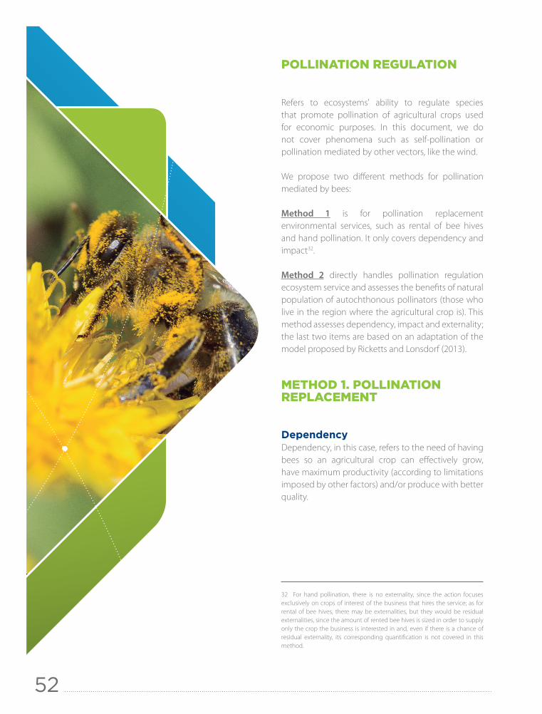
52

POLLINATION REGULATION

Refers to ecosystems' ability to regulate species that promote pollination of agricultural crops used for economic purposes. In this document, we do not cover phenomena such as self-pollination or pollination mediated by other vectors, like the wind.

We propose two different methods for pollination mediated by bees:

Method 1 is for pollination replacement environmental services, such as rental of bee hives and hand pollination. It only covers dependency and impact32.

Method 2 directly handles pollination regulation ecosystem service and assesses the benefits of natural population of autochthonous pollinators (those who live in the region where the agricultural crop is). This method assesses dependency, impact and externality; the last two items are based on an adaptation of the model proposed by Ricketts and Lonsdorf (2013).

METHOD 1. POLLINATION REPLACEMENT

DependencyDependency, in this case, refers to the need of having bees so an agricultural crop can effectively grow, have maximum productivity (according to limitations imposed by other factors) and/or produce with better quality.

32 For hand pollination, there is no externality, since the action focuses exclusively on crops of interest of the business that hires the service; as for rental of bee hives, there may be externalities, but they would be residual externalities, since the amount of rented bee hives is sized in order to supply only the crop the business is interested in and, even if there is a chance of residual externality, its corresponding quantification is not covered in this method.

53

Quantification:

Physical metric: DPacj = [(GPbpacj/Mpacj) - 1] x 100

Where: DPacj = Dependency of agricultural crop j on bee pollination, as a percentage

GPbpacj = Gain of productivity with bee pollination of an agricultural crop j in its usual physical unit of measurement (tons, etc.) and per ha

Mpacj = Maximum productivity of an agricultural crop j in its usual physical unit of measurement (tons, etc.) and per ha

Estimating GPbpacj is critical to analyze the economic importance of pollination. Estimates for certain crops can be found in specialized literature and, in case there is no publication on the topic, the estimation can be performed through field experiments.

ValuationThe valuation method adopted is the Replacement Cost Method (Annex 1), which, in this case, estimates pollination replacement costs for part of the agricultural crop productivity that depends upon pollination.

Value of the dependency = Effpr x $dcpr x Ajn + $icpr

Where: Effpr = Effort needed for complete pollination replacement for dependent agricultural crop j, per ha

$dcpr = Direct costs incurred in the pollination replacement efforts, per ha and per Effpr unit

Ajn = N area of agricultural crop j $icpr = Indirect costs of pollination

replacement

The effort for pollination replacement, Effpr, can be measured by the number of rented bee colonies, working hours in hand pollination, or other proper units of measurement.

Direct costs of this effort, $dcpr, refer to the cost of renting bee hives, working hours in hand pollination, material and equipment that are critical to replace pollination (pollen, for hand pollination, etc.), among others.

Indirect costs of pollination replacement, $icpr, include all expenses needed to support and ensure pollination replacement, such as: maintenance costs, transport and installation of rented bee colonies, costs incurred in accommodation, feeding and transport of workers somehow related to the effort of pollination replacement, among other costs that might be relevant.

ImpactImpact in this case refers to the consequences in the variation of pollination availability for the business, i.e.; variation in productivity, quality and other agricultural production characteristics somehow related to pollination mediated by bees.

QuantificationQuantification in this case is based on the effort made to replace wild pollination, either by importing pollinators, or by using hand pollination in specific agricultural crops.

Physical metric: Ipacj = Qpr/Ajn

Where: Ipacj = Impact of pollination on agricultural crop j

Qpr = Quantity of pollination replacement, which can be measured in rented bee colonies, or working hours dedicated to hand pollination

Ajn = N area of agricultural crop j

ValuationThe valuation method adopted is the Replacement Cost Method (Annex 1), which, in this case, estimates pollination replacement costs for part of the agricultural crop productivity that depends upon pollination and that was actually lost or can be lost under certain circumstances relevant to the analysis.

Value of the impact = Ipacj x $dcpr x Ajn + $icpr

54

METHOD 2. WILD POLLINATION

DependencyDependency, in this case, refers to the need of having bees so an agricultural crop can effectively grow, have maximum productivity (according to limitations imposed by other factors) and/or produce with better quality.

Quantification

Physical metric: DPacj = [(GPbpcaj/Mpacj) - 1] x 100

Where: DPacj = Dependency of agricultural crop j on bee pollination, as a percentage

GPbpacj = Gain of productivity with bee pollination of an agricultural crop j in its usual physical unit of measurement (tons, etc.) and per ha

Mpacj = Maximum productivity of an agricultural crop j in its usual physical unit of measurement (tons, etc.) and per ha

Estimating GPbpacj is critical to analyze the economic importance of pollination. Estimates for certain crops can be found in specialized literature and, in case there is no publication on the topic, the estimation can be performed through field experiments.

ValuationThe valuation method adopted is the Marginal Productivity Method (Annex 2), which, in this case, estimates the economic value of pollination through the monetary value associated to the production portion that depends on pollination.

Value of the dependency = Mpacj x DPcaj x Ajn x $acj

Where: Mpacj = Maximum productivity of an agricultural crop j in its usual physical unit of measurement (tons, etc.) and per ha

Ajn = N area of agricultural crop j, using the same unit of measurement as Mpacj area

$acj = Selling price of the agricultural crop j, in BRL, using the same physical measurement unit as Mpacj

Ideally, Mpacj should be determined through field experiments, but, alternatively, you can use data from specialized literature or maximum productivity observed previously in the region.

ImpactImpact, in this case, refers to the consequences in the variation of bee availability for the business conducting the analyses, i.e.; variation in productivity, quality and other agricultural production characteristics somehow related to pollination mediated by bees.

QuantificationQuantification, according to the method based on Ricketts and Lonsdorf (2013), is performed in three steps. The first two steps are preliminary and support a third step, in which a dose-response function is built to actually estimate the impact.

Step 1 – Diagnosis of Pollinators Diversity in Areas where Pollinators Live

The diagnosis of pollinators diversity in each area is based on two critical metrics: wealth and abundance.

Wpm = Wealth = number of pollinator species in area m

Apim = Abundance = number of specimen (individuals) from

species i in area m, per ha

55

Both Wpm and Apim shall be directly estimated from samples in the field. If more than one area is considered in the study, i.e.; m > 1, it is desirable to also show the wealth and abundance of pollinators in those areas. But, if it is not possible to do so, wealth and abundance from those areas can be indirectly estimated, according to Kennedy et al (2013). DEVESE33 calculation tool can estimate that.

Ideally, all areas with potential to supply pollinators within a 10-km-(6.2-mile-) range of pollination-dependent (either native or anthropic) areas, should be assessed. This includes areas that are not under the business or their suppliers' operational control, since pollination-dependent areas can receive bees from surrounding areas, regardless of who controls them. Nevertheless, methodological procedures indicated here can estimate only contributions from individual areas, and then you can sum up contributions from areas controlled by the business.

Finally, at the end of this step, there should be data available on pollinators wealth and abundance from areas sampled in the field, as well as their corresponding estimates for other relevant areas that were not sampled.

Step 2 – Estimate of Pollinators Diversity in Pollination-Dependent Areas n

Pollinators have a limited range, meaning there is a maximum distance they can go in their search for pollen. You need to assess, based on the source areas (m) analyzed in Step 1 and the distance between those areas and pollination-dependent areas n, which pollinator species can actually reach those areas n and how abundant they are.

As this step assesses the consequences for the business of variations in pollinator availability, pollination-

dependent areas n should be areas under the business or their suppliers' (value chain's) operational control.

Apjin = ∑M APji x 2.7183-dmn/di

Apjn = ∑Wpj APjin

Apn = Apjn/Ajn

Where: Apjin = Abundance of pollinator from agricultural crop j, belonging to species i, in pollination-dependent area n

Apji = Abundance of pollinator from agricultural crop j, belonging to species i, in area m, where m ranges from 1 to M when M > 1

dmn = Distance from area m, where pollinators are from, to area n, which is pollination-dependent

di = Maximum travel distance of pollinator from species i

Apjn = Abundance of pollinators from agricultural crop j in pollination-dependent area n (having already summed up pollinators from all species found in areas m)

Wpj = Wealth of pollinators for agricultural crop j

Apn = Abundance of pollinators in area n per hectare

Ajn = Area where agricultural crop j is, in ha

Step 2 shall be repeated for each area n, that is, for each pollination-dependent area included in the analysis.

33 Available at TeSE website: www.tendenciasemse.com.br

56

Distance dmn shall be measured, and measuring shall be performed from the middle of area m to the middle of area n.

Distances di can be obtained from specialized literature (GREENLEAF, WILLIAMS, WINFREE & KREMEN, 2007) and are available at DEVESE calculation tool.

The wealth of local pollinators (group of areas m or M), Wp, can be obtained in Step 1. In areas m where wealth was not sampled, for simplification purposes, you can use the same wealth found in sampled areas.

Step 3 – Influence of Pollinators in Agricultural Production

In this step, the function adopted associates pollinator availability with agricultural crop productivity, so it is a dose-response function. The dose-response function adopted here is equivalent to the generic quadratic model -ax2 + bx, where a and b are constant, and x = Apn

34.

a = - (Mpacj x DPacj/100)/Pdacj2

b = - 2 x a x Pdacj

Physical metric: Ipacj = (a x Apn2 + b x Apn)/Mpacj

Where: a = Quadratic model constant Pdacj = Estimate of pollinator density

(quantity of pollinators per hectare) needed to ensure maximum pollination of 1 ha of agricultural crop j

Mpacj = Maximum productivity of agricultural crop j

b = Quadratic model constant DPacj = Dependency of agricultural crop j on

bee pollination, as a percentage Ipacj = Impact of pollination on agricultural

crop j

If data on Pdacj cannot be found in specialized literature, it can be estimated through field experiments.

Ideally, Mpacj should be deduced based on Pdacj, through field experiments. If field experiments are not possible, you can use data from specialized literature, or adopt the maximum productivity observed previously in the region.

ValuationThe valuation method adopted is the Marginal Productivity Method (Annex 2), which, in this case, estimates the economic value of pollination through the economic value associated to the business production portion that changed due to variation on pollinator availability.

Value of the impact = Mpacj x Ajn x $acj x Ipacj

ExternalitiesExternalities, in this case, refer to consequences of variations of pollinator availability in areas under the business operational control on third-party agricultural production areas, particularly on communities surrounding the area m that supplies pollinators and is managed by the business or by its supply chain.

QuantificationQuantification, according to the method based on Ricketts and Lonsdorf (2013), is performed in three steps. The first two steps are preliminary and support a third step, in which a dose-response function is built to actually estimate the impact. It is the same model described for quantifying impacts, except for two critical differences in Step 2 of the model development:

• Pollination-dependent areas n will be third-party areas within a range of up to 10 km (6.2 miles) away from areas m under the business operational control.

• Only contributions from areas m under the business operational control should be considered for pollinator availability.

34 That dose-response function model is different from the model used by Rickets & Lonsdorf (2013). It was selected because it is simpler and easier when it comes to build parameters, and its adherence to pollination ecological processes is supposedly as good as the model adopted by Rickets & Lonsdorf (2013), although neither of those models was actually sufficiently studied on that matter.

57

Step 1 – Diagnosis of Pollinators Diversity in Areas m where Pollinators Live

The diagnosis of pollinators diversity in each area is based on two critical metrics: wealth and abundance.

Wpm = W = number of pollinator species in area m Apim = Abundance = number of specimen (individuals) from

species i in area m, per ha

Both Wpm and Apim shall be directly estimated from samples in the field, in the area to be studied (please remember only areas under the business operational control should be considered). If more than one area is considered in the study, i.e.; m > 1, it is desirable to also show the wealth and abundance of pollinators in those areas. But, if it is not possible to do so, wealth and abundance from those areas can be indirectly estimated, according to Kennedy et al (2013). DEVESE35 calculation tool can estimate that.

Ideally, all areas with potential to supply pollinators within a 10-km-(6.2-mile-)range of pollination-dependent (either native or anthropic) areas, should be assessed. Nevertheless, methodological procedures indicated here can estimate only contributions from individual areas, and then you can sum up contributions from areas controlled by the business.

Finally, at the end of this step, there should be data available on pollinators wealth and abundance from areas sampled in the field, as well as their corresponding estimates for other relevant areas that were not sampled.

Step 2 – Estimate of Pollinators Diversity in Pollination-Dependent Areas n

Pollinators have a limited range, meaning there is a maximum distance they can go in their search for pollen.

You need to assess, based on the source areas (m) analyzed in Step 1 and the distance between those areas and pollination-dependent areas n, which pollinator species can actually reach those areas n and how abundant they are.

As this step assesses the consequences for third-parties of variations in pollinator availability in areas m controlled by the business or its value chain, pollination-dependent areas n should be areas under those stakeholders' control, rather than under the business or its value chain's control.

Apjin = ∑M APji x 2.7183-dmn/di

Apjn = ∑Wpj APjin

Apn = Apjn/Ajn

Where: Apjin = Abundance of pollinator from agricultural crop j, belonging to species i, in pollination-dependent area n

Apji = Abundance of pollinator from agricultural crop j, belonging to species i, in area m, where m ranges from 1 to M when M > 1

dmn = Distance from area m, where pollinators are from, to area n, which is pollination-dependent

di = Maximum travel distance of pollinator from species i

Apjn = Abundance of pollinators from agricultural crop j in pollination-dependent area n (having already summed up pollinators from all species found in areas m)

Wpj = Wealth of pollinators for agricultural crop j

Apn = Abundance of pollinators in area n per ha

Ajn = Area n where agricultural crop j is, in ha

35 Available at TeSE website: www.tendenciasemse.com.br

58

Step 2 shall be repeated for each area n, that is, for each pollination-dependent area included in the analysis.

Distance dmn shall be measured, and measuring shall be performed from the middle of area m to the middle of area n.

Distances di can be obtained from specialized literature (GREENLEAF et al, 2007) and are available at DEVESE calculation tool.

The wealth of local pollinators (group of areas m or M), Wp, is the same value obtained in Step 1. In areas m where wealth was not sampled, for simplification purposes, you can use the same wealth found in sampled areas.

Step 3 – Influence of Pollinators in Agricultural Production

In this step, the function adopted associates pollinator availability with agricultural crop productivity, so it is a dose-response function. The dose-response function adopted here is equivalent to the generic quadratic model -ax2 + bx, where a and b are constant, and x = Apn

36.

a = - (Mpacj x DPacj/100)/Pdacj2

b = - 2 x a x Pdacj

Physical metric: Epacj = (a x Apn2 + b x Apn)/Mpacj

Where: a = Quadratic model constant Pdacj = Pollinator density (pollinators/

ha) needed to ensure maximum pollination of 1 ha of agricultural crop j

Mpacj = Maximum productivity of agricultural crop j

b = Quadratic model constant DPacj = Dependency of agricultural crop j on

bee pollination, as a percentage Epacj = Externality produced by pollinating

agricultural crop j.

Similarly to what happens for impact analysis, the major challenges in analyzing externalities lay on obtaining estimates for Mpacj and Dpacj.

But, for externalities, it is a little more challenging, because you are not sure you will be allowed to access pollination-dependent agricultural areas, since they belong to third-parties.

If you cannot empirically determine Mpacj and Dpacj through experiments, then you will need to obtain those estimates from specialized literature, or even from experts' opinion.

ValuationThe valuation method adopted is the Marginal Productivity Method (Annex 2), which, in this case, estimates the economic value of pollination through the economic value associated to the third-party production portion that changes due to variation on availability of pollinators from areas m under the business' or its value chain's operational control.

Value of the externality = Mpacj x Ajn x $acj x Epacj

Where: Mpacj = Maximum productivity of an agricultural crop j in its usual physical unit of measurement (tons, etc.) and per ha

Ajn = N area of agricultural crop j, using the same unit of measurement as Mpacj area

$acj = Selling price of the agricultural crop j, in BRL, using the same physical measurement unit as Mpacj

36 That dose-response function model is different from the model used by Rickets & Lonsdorf (2013). It was selected because it is simpler and easier when it comes to build parameters, and its adherence to pollination ecological processes is supposedly as good as the model adopted by Rickets & Lonsdorf (2013), although neither of those models was actually sufficiently studied on that matter.

59

Important RemarksThe Replacement Cost Method (RCM) used in method 1 tends to generate minimum value estimates linked to ecosystem services (please refer to Annex 1). The maximum value, in this case, would be equivalent to the price of what could not be produced due to no pollination replacement.

The quadratic method adopted in method 2 implies decrease in productivity after reaching its peak. Such decrease matches the results of recent researches on the ecological process of pollination mediated by animals; nevertheless, it was limited to 10% of the peak value, since there is no accurate data about the real size of this decrease37.

Investments needed to estimate pollinator diversity (Wp and Ap), productivity at peak pollination levels (Mpacj), density of pollinators needed to ensure maximum agricultural crop pollination (Pdacj) and productivity with bee pollination (GPbpacj) are not high, and the time required to conduct field experiments for this purpose is usually the reproductive cycle of the agricultural crop that is going to be analyzed. Moreover, Mpacj, Pdacj and GPbpacj can be used in future reassessments, so they do not need to be reassessed every year. As for Wp and Ap, variables that are easily accessible, if applicable, can be adjusted to land use change in the region, with no need for a new diagnosis. Ideally, though, diagnosis of pollinator diversity should be regularly performed; annually, if possible.

The model used does not take into account information about pollinator preferences for a certain type of plant, or the efficiency of different species in the pollination process for specific agricultural crops.

The model adopted here is similar to the one used by InVEST, which works with digital maps. Therefore, InVEST pollination module can be used to replace the guidelines presented here.

37 TeSE calculation tool will automatically make this adjustment.

60

Box 12. Example: Pollination RegulationMethod 1. Pollination Replacement

A small agricultural business owns two properties about 15 km (9.3 miles) away from each other. In area A, it grows coffee in 100 ha, and in area B it grows passion fruit in 1 ha.

The areas are surrounded by lands that were recently prepared for pastureland, therefore they do not count with wild bee populations.

DEPENDENCYBee pollination contributes to up to 33% of the productivity in a coffee plantation, and 75% of the productivity in a passion fruit plantation.

In order to ensure production in area A, the business would need 2 Apis mellifera honey bee colonies for each hectare of planted area per blooming. Rental price is BRL 100.00 per colony, and indirect costs of transportation, installation and maintenance of the colonies and related labor total BRL 2,500.00.

However, to ensure production in area B, the business decided to hire hand pollination services. Estimates were they would need 200 h of work to pollinate the productive area, at a cost of BRL 50.00/h. Indirect costs for extracting and preparing pollen, as well as transporting, accommodating and feeding the workers totaled BRL 2,000.00.

Quantification

Physical metric: Coffee: DPaccoffee = 33% Passion fruit: DPacpassion fruit = 75%


Coffee = Effpr x $dcpr x Ajn + $icpp = 2 x 100 x 100 + 2,500.00 = BRL 22,500.00

Passion fruit = Effpr x $dcpr x Ajn + $icpr = 200 x 50 x 1 + 2,000.00 = BRL 12,000.00

IMPACTIn the last bloom period, however, the business managed to rent only one bee colony/ha for area A, with indirect costs of BRL 1,500.00, and was only able to hire workers for the equivalent to 150 h work/ha for area B, with indirect costs summing up BRL 1,700.00.

Quantification

Physical metric: Area A: Ipacj = Qpr/Ajn = 1 bee colony Area B: Ipacj = Qpr/Ajn = 150 working hours/ha

Value of the impact:

Area A: Ipacj x $dcpr x Ajn + $icpr = 1 x 100 x 100 + 1,500.00 = BRL 11,500.00

Area B: Ipacj x $dcpr x Ajn + $icpr = 150 x 50 x 1 + 1,700.00 = BRL 9,200.00

Method 2. Wild Pollination

A coffee export business controls a farm with 100 ha of coffee plantation. In their property, there are 15 ha of preserved tropical forest fragments (FF1), whereas in the surroundings, in a 10-km- (6.2-mile) distance, there are three other forest fragments, two of them with the same characteristics, measuring 5 (FF2) and 20 (FF3) ha respectively, and a third fragment that is degraded, measuring 3 ha (FF4). Experiments have shown coffee productivity in the region is 33% dependent on pollination, and the maximum productivity on the farm was estimated to be 2.5 t/ha. Coffee average selling price is BRL 466.67/t.

Please refer to Appendix 3 to see further details of impact and externality calculations.

DEPENDENCY

Quantification

Physical metric: DPaccoffee = 33%


Mpaccoffee x Acoffee x $accoffee x DPaccoffee = 2.5 x 100 x 466.67 x 0.33 = BRL 38,500.28

IMPACTThree coffee pollinator species were identified in FF1 area: Apis mellifera (A. mellifera), Melipona fasciata (M. fasciata), and Tetragonisca angustula (T. angustula), with the following corresponding densities (specimens/ha): 30,000, 20,000, and 10,000. There are other potential three areas to provide pollinators: FF2, FF3, and FF4.

61

QuantificationStep 1

FF1: Wpm = 3 (A. mellifera, M. fasciata, and T. angustula) Apm= 30,000 (A. mellifera), 20.000 (M. fasciata), and

10,000 (T. angustula)

For FF2 and FF3, we assumed the same Wpm as for FF1, and abundance estimate was indirect.

As characteristics of vegetation in FF1 are equivalent to vegetation in FF2 and FF3, bee abundance per hectare in FF2 and FF3 will be the same as for FF1. As for FF4, as vegetation is degraded when compared to FF1, bee abundance was adjusted:

FF4: Apam = 30,000/(1+ (0.71 - 0.53)/ 0,1 x 0.232) = 21,163/ha Apmf = 20,000/(1 + (0.71 - 0.53)/ 0,1 x 0.232) = 14,108/ha Apta = 10,000/(1+ (0.71 - 0.53)/ 0.1 x 0.232) = 7,054/ha

Step 2Distances between coffee plantation and forest remnants are: 100 m (328 ft) to FF1, 1,000 m (3,280 ft) to FF2, 7,350 m (24,114 ft) to FF3, and 5,300 m (17,388 ft) to FF4.

As FF3 is located beyond the flight distance of the three pollinator species identified in the region (GREENLEAF et al, 2007), it does not contribute to pollinate coffee on the farm (only area n in this example).

Apjn = ApAm + ApMf + ApTa = 594,907 + 331,994 + 130,032 = 1,056,933 specimens

Apn = Apjn/Ajn = 1,056,933/100 = 10,569 specimens/ha

Step 3The amount of pollinators to ensure effective pollination of flowers in 1 ha of coffee was estimated in 50,000.

Physical metric: Ipacj = (a x Apn2 + b x Apn)/Mpacj

= (- 3.3 x 10-10 x 10,5692 + 3.3 x 10 - 5 x 10,569)/2.5 = 0.3119/2.5 = 0.1248 = 12.48%

Value of the impact

Mpaccoffee x Acoffee x $accoffee x Ipaccoffee = 2.5 x 100 x 466.67 x 0.1248 = BRL 14,560.10

EXTERNALITYOnly FF1 area is under the business operational control and, therefore, it is the only area with potential to generate externalities through pollination regulation.

Only one external production area was determined (area n, dependent on pollination and belonging to another farm), in a 10-km- (6.2-mile-) distance from FF1. That area is 10 ha long and is also used for coffee production.

QuantificationStep 1

FF1: Wp = 3 (A. mellifera, M. fasciata, and T. angustula) Ap = 30,000 (A. mellifera), 20,000 (M. fasciata), and

10,000 (T. angustula)

Step 2The distance between area n and FF1 is 900 m (0.5 mile), which is greater than the distance T. angustula can fly, so this excludes the species as a pollinator in area n.

i = A. mellifera (Am): Apin = 15 x 30,000 x 2.7183 ^ (-900/5900) = 386,335 specimens

i = M. fasciata (Mf): Apin = 15 x 20,000 x 2.7183 ^ (-900/1500) = 164,643 specimens

Apcoffee = ApAm + ApMf = (386,335 + 164,643)/10 = 55,098 specimens/ha

Step 3

Physical metric: Epacj = (a x Apn2 + b x Apn)/Mpacj

= (- 3.3 x10-10 x 55,0982 + 3.3 x10-5 x 55,098)/2.5 = 0.8164/2.5 = 0.3266 = 32.66%


Mpaccoffee x Acoffee x $accoffee x Epaccoffee = 2.5 x 10 x 466.67 x 0.3266 = BRL 3,810.03


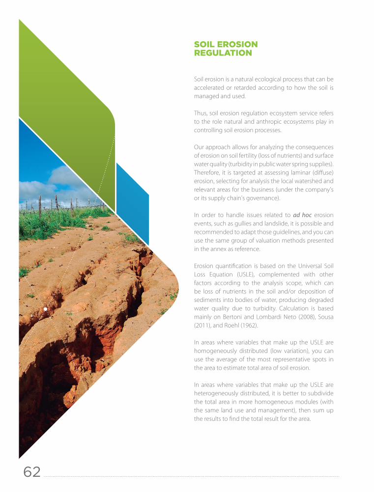
62

SOIL EROSION REGULATION

Soil erosion is a natural ecological process that can be accelerated or retarded according to how the soil is managed and used.

Thus, soil erosion regulation ecosystem service refers to the role natural and anthropic ecosystems play in controlling soil erosion processes.

Our approach allows for analyzing the consequences of erosion on soil fertility (loss of nutrients) and surface water quality (turbidity in public water spring supplies). Therefore, it is targeted at assessing laminar (diffuse) erosion, selecting for analysis the local watershed and relevant areas for the business (under the company's or its supply chain's governance).

In order to handle issues related to ad hoc erosion events, such as gullies and landslide, it is possible and recommended to adapt those guidelines, and you can use the same group of valuation methods presented in the annex as reference.

Erosion quantification is based on the Universal Soil Loss Equation (USLE), complemented with other factors according to the analysis scope, which can be loss of nutrients in the soil and/or deposition of sediments into bodies of water, producing degraded water quality due to turbidity. Calculation is based mainly on Bertoni and Lombardi Neto (2008), Sousa (2011), and Roehl (1962).

In areas where variables that make up the USLE are homogeneously distributed (low variation), you can use the average of the most representative spots in the area to estimate total area of soil erosion.

In areas where variables that make up the USLE are heterogeneously distributed, it is better to subdivide the total area in more homogeneous modules (with the same land use and management), then sum up the results to find the total result for the area.

63

DependencyDependency, in this case, occurs when the business is vulnerable to erosion processes, that is, if business can somehow be affected with economic loss should erosion processes accelerate in a certain area or relevant region for the company (including, in this case, its value chain). This will occur if the business and/or its suppliers directly or indirectly depend on soil fertility, or on quantity and quality of water, in cases conservation should be applied upstream its collection points.

In this sense, dependency is a function of maximum erosion retention that can be ensured by natural ecosystems and economically benefits the business.

QuantificationFor loss of soil nutrients, analysis shall only take into account those areas that are relevant to the business (governed by it or by its value chain). For deposition of sediments into bodies of water, the analysis should take into account areas that are located upstream the areas under the business' or its value chain's governance. Quantification is measured using the Universal Soil Loss Equation:

USLE: Se = ∑n (Ra x Ka x LSa x UMa x Aa)/Ta

Where: n = Number of areas a assessed Se = Soil erosion, in t/ha x year Ra = Rainfall erosivity factor in area a in

MJ mm/ha x h x year Ka = Soil erodibility factor in area a in t x

h/MJ x mm LSa = Length of slope factor (combination

between length and slope angle in a certain area) in area a

UMa = Land use factor (U) and management practice factor (M) in area a

Aa= Analyzed area, in ha Ta= Total area (sum of areas a), in ha.

Dependency quantification of this ecosystem service shall be performed using 2 Se estimates, one estimate with the highest erosion level UM, that is, exposed soil Semax, and another estimate with the lowest erosion level UM (maximum soil retention), that is, native vegetation cover Semin.

In case there is loss of soil nutrients, Semax and Semin are then called Semaxarea and Seminarea, as a reference to the area that is relevant to the business (area).

For deposition of sediments into bodies of water, they become Semaxu and Seminu, as a reference to upstream areas (u).

Rainfall erosivity, R, can be obtained from average annual pluviosity and rainfall intensity, according to Bertoni and Lombardi Neto (2008). DEVESE calculation tool presents some values obtained for different regions in Brazil that can be used as reference in case there are no local values.

K, UM and LS variables should preferably be obtained in the field. In case it is not feasible, they can be obtained from technical and scientific studies developed in the region, or you can use default values available at DEVESE calculation tool. To determine LS, lengths and slope angles shall be diagnosed in the area, in the field, or by using slope effect plots.

For Semin, you shall adopt the UM factor that corresponds to the area native vegetation.

Physical metric – Loss of Soil Nutrients: LNs = Ns x (Semaxarea - Seminarea)

Where: LNs = Loss of soil nutrients, in t/ha x year Ns = Concentration of soil nutrients, in t/

ha Semaxarea = Soil erosion in t/ha per year, as soil

exposed in areas that are relevant to the business

Seminarea = Soil erosion in t/ha per year, as soil covered by the region native vegetation, in areas that are relevant to the business

Ns value shall be determined based on local data, through laboratory analysis. Whenever it is not possible to get local data, you can use secondary data from similar soils.

a = 1

64

Physical metric – turbidity in the body of water

Turbidity, whenever there are no local studies to determine it through association with current concentration of suspended sediments, can be defined as:

Tbw = (ln(RSD x (Semaxu - Seminu) x 31.7098 x Ta/Falt) - 1.57)/0.1

Where RSD = 771.8448 x (Difalt/Lmbw)0.83291

Where: Tbw = Turbidity in the body of water, in UTN RSD = Rate of sediment deposition

(percentage) Semaxu = Soil erosion as soil exposed

upstream, in t/ha x year Seminu = Soil erosion as soil covered by

the region native vegetation, in upstream areas, in t/ha x year

Falt = Average long-term water flow, in L/s (L/s=(m3/s) x 1000)

Ta = Total area, in ha Difalt = Difference between maximum

and minimum altitudes in area a upstream, in m

Lmbw= Length of main body of water in the area, in m

Both Difalt and Lmbw shall be obtained in the field or deduced from plots or satellite imagery. Falt can be measured in the field or obtained from reports and specialized technical studies, as the ones produced by watershed agencies or other public bodies in charge of granting licenses.

It is worth pointing out that Tbw does not estimate total deposition of turbidity into the body of water, but only the portion that can be controlled by ecosystem service – in practice, by managing land use.

ValuationLoss of soil nutrients – The valuation method adopted is the Replacement Cost Method (Annex 1), which, in this case, estimates expenses that would

be necessary to replace nutrients lost due to erosion processes that cause loss of productivity in agricultural crops.

Value of the dependency = $Ns x Ta + $log

Where: $Ns = Cost of soil nutrients, per ha Ta = Relevant area for the business, in ha $log = Costs with logistics to apply soil

nutrients

Turbidity in the body of water – As soil erosion, in the context of sediment deposition into a body of water, degrade water quality, the valuation method in this case is the same one adopted for water quality regulation ecosystem service. Therefore, the valuation method adopted is the Replacement Cost Method (Annex 1), which, in this case, estimates the expenses that would be necessary to recover degraded water quality should no water quality regulation ecosystem service be available.

Value of the dependency = Qwcol x $Tw + Iwtp


$Tw = Cost of water treatment to remove Tbw up to an acceptable level for the business, in BRL/m3


Qwcol variable shall be obtained from measurements performed by the business operational area. $Tw and Iwtp can also be obtained with the business operational area, or quoted in the water treatment service market.

This dependency valuation method is also applied to businesses that buy treated water; all you need to do is replace $Tw + Iwtp components in the above formula with the price paid for the water.

ImpactImpact occurs only if the business is vulnerable to erosion processes, that is, if business can somehow be affected with economic loss should erosion processes accelerate in a relevant area for the company (including, in this case, its value chain).

65

In this sense, impact here is an economic outcome for the business of loss or reduction of ecological processes that cause soil retention and, consequently, control erosion processes.

QuantificationWhereas for dependency quantification would be the result from the difference between maximum and minimum soil retention through ecological processes, for impact quantification will be calculated by the difference between current (real) and maximum soil retention level through ecological processes.

For loss of soil nutrients, analysis shall only take into account those areas that are relevant to the business (governed by it or by its value chain). For deposition of sediments into bodies of water, the analysis should take into account areas that are located upstream the areas that are relevant to the business.

Quantification of the impact associated with loss or reduction of this ecosystem service shall be performed with two Se estimates: one with current (real) UM standards, that provide current erosion level, Securrent, and the other with maximum protection against erosion UM, meaning native vegetation cover – minimum levels of soil erosion Semin.

In case there is loss of soil nutrients, Securrent and Semin are then called Securrentarea and Seminarea, as a reference to the area that is relevant to the business (area).

For deposition of sediments into bodies of water, they become Securrentu and Seminu, as a reference to upstream areas (u).

Physical metric – Loss of Soil Nutrients: LNs = Ns x (Securrentarea - Seminarea)

Where: Securrentarea = Soil erosion in current (real) conditions of land use in areas that are relevant to the business, in t x ha/year


Tbw = (ln(RSD x (Securrentu - Seminu) x 31.7098 x Ta/Falt) - 1.57)/0.1


Where: Securrentu = Soil erosion in current conditions of land use in upstream areas, in t/ha x year

ValuationLoss of soil nutrients – The valuation method adopted is the Replacement Cost Method (Annex 1), which, in this case, estimates expenses that would be necessary to replace nutrients lost due to erosion processes.

Value of the impact = $Ns x Arec + $log

Where: Arec = Area to be recovered, in ha

Turbidity in the body of water – As soil erosion, in the context of sediment deposition into a body of water, degrade water quality, the valuation method in this case is the same one adopted for water quality regulation ecosystem service. Therefore, the valuation method adopted is the Replacement Cost Method (Annex 1), which, in this case, estimates the expenses that would be necessary to recover degraded water quality should no soil erosion regulation ecosystem service be available.

Value of the impact = Qwcol x $Tw + Iwtp

ExternalityExternality will only occur if any water user downstream the relevant areas to the business is vulnerable to erosion processes, i.e.; if there is any economic loss should natural erosion processes accelerate in areas that are relevant to the business (areas under the company's or its suppliers' governance, varying according to the scope of the analysis).

In this sense, externality here is the economic outcome for downstream water users of loss or reduction of ecological processes that cause soil retention in areas that are relevant to the business.

66

It is not considered externality when it comes to loss of soil nutrients, since in areas relevant to the business it is the business itself that is affected by those losses and, thus, it is considered an impact, not an externality. Eventual impacts that may be caused by soil nutrient deposition downstream are considered degraded water quality, and are covered directly by methods targeted at that ecosystem service.

QuantificationWhereas for dependency and impact the analysis focus on areas located upstream the areas that are relevant to the business, for externalities the analysis focus only on areas that are relevant to the business.

USLE: Se = ∑n (Ra x Ka x LSa x UMa x Aa)/Ta

Where: n = Number of areas a assessed Se = Soil erosion, in t/ha x year Ra = Rainfall erosivity factor in area a in

MJ mm/ha x h x year Ka = Soil erodibility factor in area a in t x

h/MJ x mm LSa = Length of slope factor (combination

between length and slope angle in a certain area) in area a

UMa = Land use factor (U) and manage-ment practice (M) factor in area a

Aa= Analyzed area, in ha Ta= Total area (sum of areas a), in ha.

Quantification of the externality associated with loss or reduction of this ecosystem service shall be performed with two Searea estimates exclusively for areas that are relevant to the business: one with current (real) UM standards, related to the current erosion level, Securrentarea, and the other, either hypothetical or real, with maximum protection UM, meaning native vegetation cover Seminarea.

Rainfall erosivity, R, can be obtained from average annual pluviosity and rainfall intensity, according to Bertoni and Lombardi Neto (2008). DEVESE calculation tool presents some values obtained for different regions in Brazil that can be used as reference in case there are no local values.

K, UM and LS variables should preferably be obtained in the field. In case it is not possible, they can be

obtained from technical and scientific studies developed in the region, or you can use default values available at DEVESE calculation tool. To determine LS, lengths and slope angles shall be diagnosed in the area, in the field, or by using slope effect plots.

For Semin, you shall adopt the UM factor that corresponds to the area native vegetation, free of management.

Physical metric – turbidity in the body of waterTbw = (ln(RSD x (Securrentarea - Seminarea) x 31.7098 x Ta/Falt) - 1.57)/0.1


Where: Tbw = Turbidity in the body of water, in UTN RSD = Rate of sediment deposition

(percentage) Securrentarea = Soil erosion in current conditions

of land use in areas that are relevant to the business, in t/ha x year

Seminarea = Soil erosion as soil covered by the region native vegetation, in areas that are relevant to the business, in t/ha x year

Falt = Average long-term water flow, in L/s (L/s=(m3/s) x 1000)

Ta = Total area, in ha Difalt = Difference between maximum

and minimum altitudes in area a upstream, in m

Lmbw= Length of main body of water in the area, in m

Both Difalt and Lmbw shall be obtained in the field or deduced from plots or satellite imagery. Falt can be measured in the field or obtained from reports and specialized technical studies, as the ones produced by watershed agencies or other public bodies in charge of granting licenses.

It is worth pointing out that Tbw does not estimate total deposition of sediments into the body of water, but only the portion of deposition that can be controlled by ecosystem service – in practice, by managing land use.

a = 1

67

ValuationTurbidity in the body of water – As soil erosion, in the context of sediment deposition into a body of water, degrade water quality, the valuation method in this case is the same one adopted for water quality regulation ecosystem service. Therefore, the valuation method adopted is the Replacement Cost Method (Annex 1), which, in this case, estimates the expenses that would be necessary to recover degraded water quality due to soil erosion in areas that are relevant to the business.

Value of the externality = Qwcol x $Tw + Iwtp

Where: Qwcol = Quantity of water, in m3

$Tw = Cost to treat water in order to remove Tbw up to the same level found upstream the business areas, in BRL/m3


Qwcol variable, in this specific case, refers to water collected downstream by third-parties. For practical purposes, you may assess only the first downstream water collection. $Tw and Iwtp can also be obtained with the business operational area, or quoted in the water treatment service market.

Important RemarksErosion processes also affect other ecosystem services, such as sailing38, water flow regulation39, hydropower generation40, and fishing41. Specific approaches for those ecosystem services will be developed in the future.

Quantification of erosion through USLE can be performed with different levels of accuracy, depending mainly on the relevance values assigned to USLE parameters have regarding actual environmental conditions in the area analyzed. Depending on the resources available, it is possible to use a single average value for each of those parameters, which would probably lead to less accurate estimates; use a set of average values for a group of different environmental conditions in the area analyzed, which is more likely to produce accurate results; or use ad hoc approaches, which tends to be more accurate.

Those USLE ad hoc assessment approaches can be performed with hydrological models based on geographic information systems (GIS, satellite images and the like) that can assess USLE in smaller area units (pixels). InVEST42 is a good example of that type of model. It is a free software that makes analyses with methods that are equivalent to the ones presented here. Thus, it can be adopted combined with these guidelines, or even replace them.

If you choose to use USLE in a simplified way, only in more representative spots of the area/watershed, we recommend choosing spots with: (a) higher declivity; (b) higher level of soil exposure and degradation; and (c) areas where management leaves soil frequently exposed to rain (non-perennial agricultural crops, rural roads, etc.).

RSD and Tbw calculations are based on empiric equations, developed from data collected in the field from different watershed groups. Ideally, the equation should be developed according to the watershed being studied. Applying equations developed for a certain watershed in other watersheds is like 'transferring functions', and this procedure is subject to distortions in RSD and Tbw estimates. The greater the differences in environmental conditions between the watershed used to develop the equations and the watershed being studied, the greater the distortions.

Investments on WTP can be amortized following traditional accounting criteria.

38 Silting of navigation channels and the resulting reduction in the distance between the vessel's keel and river bottom, or depth of the water column, which limits access of larger vessels.39 Silting of rivers, with resulting reduction in water flow and storage, increasing risks of floods in rainy seasons and water shortage in dry seasons.40 Silting and the resulting decrease in hydroelectric power plant reservoir storage capacity, reducing reservoir life cycle and the plant hydropower potential.41 Increase in water turbidity changes environmental conditions in the body of water and may cause reduction or even loss in local fish stocking.42 InVEST: Integrated Valuation of Ecosystem Services and Trade-offs. The Natural Capital Project: www.naturalcapitalproject.org/InVEST.html

68

Box 13. Example: Soil Erosion RegulationA business manages a 100 ha area within a 6,000 ha watershed. Out of that total, 1,100 ha are located upstream the business facilities: 800 ha of degraded pastureland (dp), which had to be subdivided into 2 subclasses because they had different lengths of slope LS (dp1 200 ha, and dp2 600 ha), 100 ha of preserved pastureland (pp), 150 ha of preserved forest remnants (pf ), and other 50 ha of urban area (ua).

The company area is subdivided as follows: in 70 ha the company raises beef cattle, and half of this area has degraded pastureland, whereas the other half is covered with preserved pastureland; 20 ha of the area are preserved as a legal reserve and as a permanent preservation area; and in the remaining 10 ha there is a meat processing plant, as well as other administrative facilities. Erosion processes compromise pastureland fertility, besides degrading the quality of the water the business collects in order to process meat – the business requires 150,000 m3 of drinking water per year for those industrial processes.

Rainfall erosivity factor R, in this case, is the same for the entire watershed: 4,865 MJ x mm/ha x h x year. As for erodibility, two key types of soil were identified with K factor of 0.047 and 0.057 t x h/MJ x mm. Lenght of slope LS factors varied as follows: ua = 7.47; pp = 11.56; dp1 = 12.27; dp2 = 15.33, and pf = 15.33.

Land use and management factor UM for exposed soil and native vegetation cover, degraded pastureland and preserved pastureland are 1 and 0.01, 0.25 and 0.12, respectively.

Please refer to Appendix 4 to see further details of calculations.

DEPENDENCY

Quantification

Physical metric – Loss of Soil Nutrients

Ns for nitrogen = 0.01 t/ha Ns for phosphor = 0.005 t/ha

Semaxarea = (92,513.81 + 98,195.89)/(35 + 35) = 2,724.42 t/ha x year Seminarea = (925.14 + 981.96)/(35 + 35) = 27.24 t/ha x year

LNs nitrogen = 0.01 x (2,724.42 - 27.24) = 26.97 t/ha x year LNs phosphor = 0,005 x (2.724,42 - 27,24) = 13,49 t/ha x year


Semaxu = (103,573.42 + 264,325.18 + 561,119.37 + 2,103,168.69 + 525,792.17)/(50 + 100 + 200 + 600 + 150) = 3,234.53 t/ha x year Seminu = (1,035.73 + 2,643.25 + 5,611.19 + 21,031.69 + 5,257.92)/(50 + 100 + 200 + 600 + 150) = 32.35 t/ha x year

The measured length of the main body of water in the watershed is 40 km (24.8 miles), and maximum and minimum altitudes are 1,000 m (3,280 ft) and 200 m (656 ft), respectively. Average estimated flow per year is 5 m3/s (5,000 l/s).

RSD = 771.8448 x (Difalt/Lmbw)0.83291 = 771.8448 x (800/40,000)0.83291 = 29.68%

Tbw = (ln(RSD x (Semaxu - Seminu) x 31.7098 x Ta/Falt) - 1.57)/0.1 = (ln(0.2968 x (3,234,53 - 32.35) x 31.7098 x 1,100/5000) - 1.57)/0.1 = 72.29 UTN

Value of the dependency – Loss of Soil Nutrients

Replacement of nitrogen and phosphor in this case was conducted by using a single fertilizer at the cost of BRL 150.00/ha, with logistics costs estimated as BRL 24,500.00.

Value of the dependency = $Ns x Ta + $log = BRL 150.00 x 70 + BRL 24,500.00 = BRL 35,000.00

Value of the dependency – turbidity in the body of water

Variable costs for water treatment, needed to reduce turbidity to less than 40 UTN were estimated as BRL 0.035/m3. The business already operates a WTP, and its annual fixed costs on operations are BRL 100,000.00.

Value of the dependency = Qwcol x $Tw + Iwtp = 150,000 x 0.035 + 100,000 = BRL 105,250.00

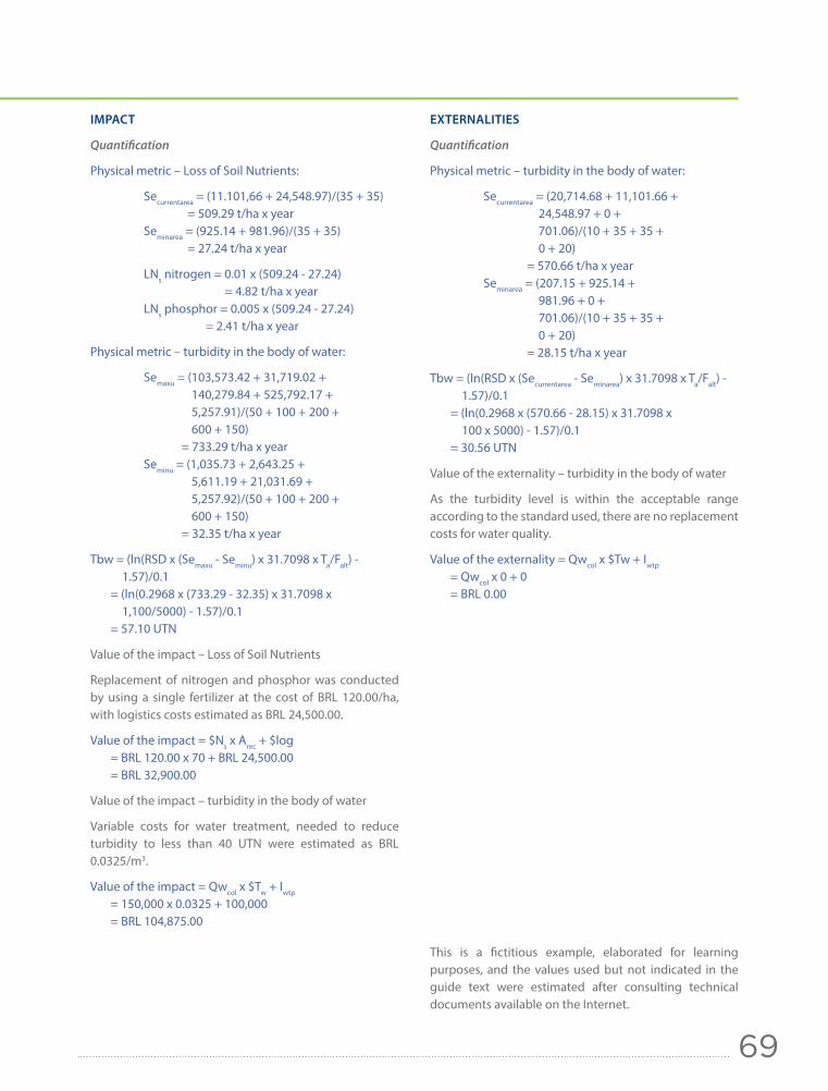
69

IMPACT

Quantification

Physical metric – Loss of Soil Nutrients:

Securrentarea = (11.101,66 + 24,548.97)/(35 + 35) = 509.29 t/ha x year Seminarea = (925.14 + 981.96)/(35 + 35) = 27.24 t/ha x year

LNs nitrogen = 0.01 x (509.24 - 27.24) = 4.82 t/ha x year LNs phosphor = 0.005 x (509.24 - 27.24) = 2.41 t/ha x year

Physical metric – turbidity in the body of water:

Semaxu = (103,573.42 + 31,719.02 + 140,279.84 + 525,792.17 + 5,257.91)/(50 + 100 + 200 + 600 + 150) = 733.29 t/ha x year Seminu = (1,035.73 + 2,643.25 + 5,611.19 + 21,031.69 + 5,257.92)/(50 + 100 + 200 + 600 + 150) = 32.35 t/ha x year

Tbw = (ln(RSD x (Semaxu - Seminu) x 31.7098 x Ta/Falt) - 1.57)/0.1 = (ln(0.2968 x (733.29 - 32.35) x 31.7098 x 1,100/5000) - 1.57)/0.1 = 57.10 UTN

Value of the impact – Loss of Soil Nutrients

Replacement of nitrogen and phosphor was conducted by using a single fertilizer at the cost of BRL 120.00/ha, with logistics costs estimated as BRL 24,500.00.

Value of the impact = $Ns x Arec + $log = BRL 120.00 x 70 + BRL 24,500.00 = BRL 32,900.00

Value of the impact – turbidity in the body of water

Variable costs for water treatment, needed to reduce turbidity to less than 40 UTN were estimated as BRL 0.0325/m3.

Value of the impact = Qwcol x $Tw + Iwtp = 150,000 x 0.0325 + 100,000 = BRL 104,875.00

EXTERNALITIES

Quantification

Physical metric – turbidity in the body of water:

Securrentarea = (20,714.68 + 11,101.66 + 24,548.97 + 0 + 701.06)/(10 + 35 + 35 + 0 + 20) = 570.66 t/ha x year Seminarea = (207.15 + 925.14 + 981.96 + 0 + 701.06)/(10 + 35 + 35 + 0 + 20) = 28.15 t/ha x year

Tbw = (ln(RSD x (Securrentarea - Seminarea) x 31.7098 x Ta/Falt) - 1.57)/0.1 = (ln(0.2968 x (570.66 - 28.15) x 31.7098 x 100 x 5000) - 1.57)/0.1 = 30.56 UTN

Value of the externality – turbidity in the body of water

As the turbidity level is within the acceptable range according to the standard used, there are no replacement costs for water quality.

Value of the externality = Qwcol x $Tw + Iwtp = Qwcol x 0 + 0 = BRL 0.00


70

RECREATION AND TOURISM

Landscape characteristics excite people and this excitement is converted, among other things, into benefits in the form of leisure, recreation and tourism. Those characteristics refer to scenic beauty, activities such as hiking, ecotourism, and sightseeing, and bodies of water used for swimming, nautical practices, recreational fishing, and others.

Often, opportunities for leisure and ecotourism are in places owned by the business or operated by it, and there might be demand from local communities or other stakeholders for such opportunities. Take, for instance, hydropower plants reservoirs and their surroundings, and areas with logging or mining activities that have attractions such as waterfalls and hiking trails.

Opportunities for recreation, leisure and tourism, on their turn, translate into demand to visit the area, and visiting contributes to local economy, generating jobs and demand for infrastructure and services.

In the context of those guidelines, quantification analyses and economic valuation of this ecosystem service are aimed at impacts and externalities. We assume there will only be dependency if the business being assessed economically includes recreation and tourism service exploration in its mission.

ImpactsImpacts for the business in this context are basically limited to gains obtained in exploration of recreation and tourism, as well as the economic effort the business makes to preserve the area in its original configuration. Gains are usually obtained by charging admission fees, visiting licenses, or selling products or services in the visitation area, whereas effort is related to the alternative economic use that could be made of this area if it were not preserved.

71

Quantification

Physical metric (effort to preserve the area): Aeealt = Ta - Auee

Where: Aeealt = Area that could have an alternative economic exploitation, in ha

Ta = Total area preserved by the business and open for visitation, in ha

Auee = Part of the area preserved by the business unavailable for alternative economic exploitation, in ha.

To calculate Auee, you should consider Areas of Permanent Preservation (APP) and other areas whose characteristics prevent exploitation in the context of economic activities that are currently developed in the region.

Physical metric 2 (area attractiveness): Nv/P

Where: Nv = Number of visitors that go to the area P = Time period considered for counting

visitors

The number of visitors can be obtained by the business controlling access points to the area. If there is no entrance registration system, the business can ultimately hire a local organization to monitor visits (a partnership, let's say). Usually, the time frame considered to assess visitation is of one year.

ValuationTwo economic valuation methods are adopted in this case. With one of the Travel Cost Method components (Annex 6), you assess expenses made by visitors directly in the visited area; and with the Opportunity Cost Method you assess the economic effort made by the business to preserve the area. As in the first case the value obtained is a real financial income, and in the second case it refers to an economic cost that does not imply cash flow for the business, those two values will be separately presented, in such a way that they can be independently assessed.

Value of the financial impact43 = Nv/P x $Af + $DfIValue of the economic impact = - (Aeealt x $Ieaalt)

Where: $Af = Admission fee, or the like $DfI = Different incomes from tourism

exploitation $Ieaalt = Incomes from alternative economic

activity, in BRL/ha

Only the internalized part of costs and expenses with visitation is being considered. $Af calculation shall include all types of admission fees, whether for one-day visit tickets, or annual fees charged in the form of use/visitation license.

$DfI calculation shall include all additional income concerning service exploitation and selling of products to visitors.

To determine $Ieaalt, you shall take into account the alternative economic use the business could make of the area. If the business has no alternative economic use of its own for the area, you can adopt the local economic activity that, at the business discretion, or at some authority or expert discretion, after having been consulted by the business, have greater chances to occupy that area should the business not support preservation practices.

ExternalitiesExternalities, in this case, refer to the portion of benefits from recreation and tourism opportunities that was not internalized by the business. The analysis is focused only on the area attractiveness and does not take into account other impacts on the local or regional economy, because of the difficulty to gather consistent data about this topic. However, if it is possible to collect data about those externalities, the values should definitely be accounted for.

43 Only visitors who are paying shall be considered in Nv estimates.

72

Quantification

Physical metric 2 (area attractiveness): Nv/P

Where: Nv = Number of visitors that go to the area P = Time period considered for counting

visitors

The number of visitors can be obtained by the business controlling access points to the area. If there is no entrance registration system, the business can ultimately hire a local organization to monitor visits (a partnership, let's say). Usually, the time frame considered to assess visitation is of one year.

ValuationThe economic valuation method adopted is the Travel Cost Method (Annex 6), which is based on costs associated with visiting a certain place. Hence, we assume travel expenses are at least equivalent to the benefits expected from recreation and/or tourism activities. Otherwise, such expenses would have no justification, and the decision to visit the area would not be made.

Value of the externality = Nv/Px ($tci + $faci)

Where: $tci= Average individual travel costs to the visited area, in BRL

$faci= Average individual feeding and accommodation costs during the trip, in BRL

$tci calculation includes expenses incurred with the fuel consumed in the round trip, toll costs, etc. If visitors have travelled by airplane or public transportation, you should consider the ticket price and the travel cost from their final destination (where they got off ) from that means of transportation to the visited area. In case the trip had multiple destinations, you shall deduce the expenses that are not related to visiting the specific area analyzed. For such, if it is not possible to obtain information directly from visitors about the specific value for the area analyzed, you can ask them information about their itinerary and additional expenses in order to estimate the discount later on.

To calculate $faci, you shall not include expenses in the visitation area, because those will be calculated as impacts internalized by the business that runs the area ($DfI).

Important RemarksTwo other metrics can contribute to identify the relevance of leisure and ecotourism activities: % of local GDP, and number of employees associated with local leisure and tourism activities. In some cases, transfer of ecological ICMS tax can also be accounted for as positive externality, as long as the state ecological ICMS tax law considers private areas as beneficiaries of the tax transfer.

Additionally, the methods indicated in this document do not consider eventual subsidies offered by businesses to visitors, such as discounts in the admission fees, since those subsidies are usually related to social issues, rather than environmental issues, and those guidelines focus on economic environmental valuation.

In the way it was determined, this ecosystem service does not imply the value associated with scenic beauty whenever it is just passive, in other words, whenever there is no economic activity. It is not possible, for instance, to capture the value associated with the pleasure felt when someone looks at the landscape if the person lives close to the visitation area and is at home, just looking through the window of his/her own house (there is no travel involved, or purchase of products or services specifically for this kind of contemplation).

In case of retrospective valuation (inventory, for example), the total travel cost value for all visitors in a one-year-period is calculated by summing up the costs of all travels during the year considered for analysis.

If you are willing to make a prospective valuation and estimate future demands or incomes for project assessment, it will be necessary to adjust a model to estimate the demand curve per visit using a travel generation function (Annex 6).

73

Box 14. Example: Recreation and TourismIn 1999, Suzano Papel e Celulose pulp and paper business, supported by Ecofuturo Institute, selected an old eucalyptus plantation farm within its property to create a 2,800 ha park, acknowledged as an Advanced Atlantic Forest Biosphere Reserve, part of Unesco's Man and the Biosphere Program. With programs focused on environmental education, ecotourism, sustainable management of natural resources, cultivation of threatened species, and scientific researches, Parque das Neblinas received over 25,000 visitors since it was created. In 2012, more than 3,265 people visited the park.

IMPACTThe main traditional economic activity in the region are low-productivity dairy farms, with average income of BRL 2,000/ha. Out of the total park area, about 400 ha are APPs.

Average admission fee to the park is BRL 35,00. Other tourism activities (restaurants, canoeing, activities, scientific expeditions, and workshops) contributed to a total value of BRL 46,363.00 throughout the year.

Quantification

Effort to preserve the area: Aeealt = Ta - Auee = 2,800 - 400 = 2,400 ha

Area attractiveness: Nv/P = 3,265/1 = 3,265 visitors/year

Value of the financial impact

Nv/P x $Af + $DfI = (3,265/1 x 35.00) + 46,363.00 = BRL 160,638.00

Value of the economic impact

- (Aeealt x $Ieaalt) = - (2,400 x 2,000.00) = - BRL 4,800,000.00

EXTERNALITYAccording to a survey conducted by Ecofuturo Institute, 19% of visitors come from the city of Sao Paulo (115 km / 71 miles away), whereas the other 81% come from areas near the park (within a 40-km- / 25-mile-range). Those coming from Sao Paulo have to pay a toll, which costs BRL 5.40 per vehicle (round trip). They usually stay in the park for the whole day, and the survey did not determine feeding or accommodation expenses other than those directly charged by the park.

As for transportation, the survey indicates an average of 3.25 passengers per vehicle. Travel cost was estimated to be BRL 0.80/km.

Quantification

Nv/P Sao Paulo = 3,265 x 19% = 620 visitors/year

Nv/P Areas near the park = 3.265 x 81% = 2.645 visitors/year

Considering the only means of transportation to access the park is by car, and there are 3.25 passengers on average, the toll cost, and the travel cost per visitor are, respectively, BRL 5.40/3.25 = BRL 1.66, and BRL 0.80/3.25 = BRL 0.25.


Visitors from Sao Paulo: Nv/P x ($tci + $faci) = 620/1 x ([1.66 + 0.25 x 115 x 2] + 0) = BRL 36,679.20

Visitors from areas near the park: Nv/P x ($tci + $faci) = 2,645/1 x ([0.25 x 40 x 2] + 0) = BRL 52,900.00

Total value of externalities = BRL 36,679.20 + BRL 52,900.00 = BRL 89,579.20

This example was elaborated for learning purposes, using data provided by Ecofuturo Institute.

74

NEXT STEPS

INCORPORATING NATURAL CAPITAL VALUES INTO BUSINESS DECISIONS

The private sector needs to invest on understanding the benefits from nature and on translating those benefits into a language that enables to properly value them in the business context. Those benefits are not limited to environmental goods and assets. They are also related to environmental conditions that ensure provision and quality of those goods and assets, meaning they also refer to ecosystem services.

Those guidelines aim at sizing the importance of ecosystem services for business by estimating their economic value. Since other resources used by business are also assessed based on their economic values, this seems to be a proper strategy to incorporate the importance of natural capital into business decision-making processes.

Economic value, however, is only one of the value dimensions associated with natural capital. Its ecologic values - which refer to the resilience and integrity needed for ecosystems to keep service provision - and sociocultural values - related to beliefs, customs, and cultural values - should be also taken into account, so businesses can really develop strategic, effective and efficient management in sustainability.

75

Effective incorporation of natural capital in business decisions is a process that depends on investments. It is critical to develop a culture of including natural capital dimension in different areas in the business, not only in sustainability. Thus, it is necessary to invest time and a team in order to understand and enhance business relationships with natural capital, particularly business risks and opportunities, in the short-, medium-, and long-terms.

IMPROVEMENT OF METHODOLOGICAL GUIDELINES

It takes a continuous process to enhance those guidelines. When the pilot projects started, in 2014, it was possible to enhance not only the methods, but also the language used, in order to make them more complete and accessible. In the next TeSE cycles, besides revising and enhancing the guidelines, new guidelines will be developed for ecosystem services that have not been included in DEVESE yet.

IMPROVEMENT OF THE CALCULATION TOOL

In 2014, we elaborated an Excel-based calculation tool that facilitates DEVESE implementation. In addition to implementing the calculations as indicated in DEVESE, the calculation tool includes a set of secondary data that can be used for estimation purposes, should more accurate primary data be missing. The tool will keep being continuously updated, and so will DEVESE.

TRAINING TO APPLY DEVESE

The first round of pilot projects to apply DEVESE, developed in 2014, enabled TeSE team to better understand the difficulties businesses have to understand and apply this kind of methodological guidelines.

With the purpose of making DEVESE application easier and enabling businesses to internalize and gain independence to apply this tool, TeSE team will develop and offer, from 2015 on, a hands-on training on how to apply DEVESE, focusing on the use of its corresponding calculation tool.

ENVIRONMENTAL EXTERNALITY REPORT

After assessing the importance of natural capital for their business, and in order to ensure their social license to operate, organizations will have to show the society how they use increasingly fewer natural resources, which, in society's opinion, could be allocated to other purposes other than the ones desired by the businesses. In this context, TeSE developed the first version of Corporate Guidelines for Environmental Externalities Report, DEREA (in the Brazilian Portuguese acronym), targeted at externalities covered in DEVESE.

DEREA will be revised and expanded from 2015 on, with participation and support of TeSE member companies.

76

BIBLIOGRAPHYAPPLETON, A. F. (2002). How New York City used an ecosystem services strategy carried out through an urban-rural partnership to preserve the pristine quality of its drinking water and save billions of dollars and what lessons it teaches about using ecosystem services. Tokyo: Katoomba Conference.

BERTONI, J., LOMBARDI, F., NETO (2008). Conservação do Solo (Soil Conservation). (6th ed.). Sao Paulo: Ícone.

Bill # 792, as of April 2007. (2007). Rules on definition of environmental services and other matters. Brasilia, DF.

CONSTANTINO, A. F. & YAMAMURA, V. D. (2009). Redução do gasto operacional em estação de tratamento de água utilizando o PAC (Operational Expense Reduction in Water Treatment Station Using PAC). Proceedings of the Symposium on Graduation in Urban Engineering, Maringa, PR, 2.

COSTANZA, R., DE GROOT, R., SUTTON, P., VAN DER PLOEG, S., ANDERSON, S. J., KUBISZEWSKI, I., FARBER, S. & TURNER, R. K. (2014). Changes in the global values of ecosystem services. Global Environmental Change, 26, 152-158.

DAILY, H. & FARLEY, J. (2010). Ecological Economics: principle and applications (2nd ed.). Washington, DC: Island Press.

DE GROOT, R., BRANDER, L., VAN DER PLOEG, S., COSTANZA, R., BERNARD, F., BRAAT,L., CHRISTIE, M., CROSSMAN, N., GHERMANDI, A., HEIN, L., HUSSAIN, S., KUMAR, P., MCVITTIE, A., PORTELA, R., RODRIGUEZ, L.C., TEN BRINK, P. & VAN BEUKERING, P. (2012). Global estimates of the value of ecosystem and their services in monetary units. Ecosystem services, 1 (1), 50-61.

FARLEY, J. (2012). Ecosystem service: the economics debate. Ecosystem services, 1 (1), 40-49.

FUNDAÇÃO DE CIÊNCIA, APLICAÇÕES E TECNOLOGIA ESPACIAIS (FUNCATE - Foundation of Spacial Science, Applications and Technologies). (2010). Emissões de Dióxido de Carbono no Setor Uso da Terra, Mudança de Uso da Terra e Florestas (Carbon Dioxide Emissions in Land Use, Land Use Change and Forestry Sector). Second Brazilian Inventory of Anthropogenic Greenhouse Gas Emission and Removal (Reference Reports/2010), Brasilia, DF, Ministry of Science and Technology.

GREENLEAF, S. S., WILLIAMS, N. M., WINFREE, R. & KREMEN, C. (2007). Bee foraging ranges and their relationship to body size. Oecologia, 153, 589-596.

HANSON, C., RANGANATHAN, J. and FINISDORE, J. (2012). The corporate ecosystem services review: guidelines for identifying business risks & opportunity arising from ecosystem change. Washington, DC: WRI. Available at: http://www.wri.org/publication/corporate-ecosystem-services-review

INTERGOVERNMENTAL PANEL ON CLIMATE CHANGE. (2003). Good Practice Guidance for Land Use, Land-Use Change and Forestry. Japan: Global Environmental Strategies (IGES).

KENNEDY, C. M., LONSDORF, E., NEEL, M. C., WILLIAMS, N. M., RICKETTS, T. H., WINFREE, R., BOMMARCO, R., BRITTAIN, C., BURLEY, E.L., CARIVEAU, D., CARVALHEIRO, L. G., CHACOFF, N. P., CUNNINGHAM, S. A., DANFORTH, B. N., DUDENHOFFER, J., ELLE, E., GAINES, H. R., GARIBALDI, L. A., GRATTON, C., HOLZSCHUH, A., ISAACS, R., JAVOREK, S. K., JHA, S., KLEIN, A. M., KREWENKA, K., MANDELIK, Y., MAYFIELD, M. M., MORANDIN, L., NEAME, L. A., OTIENO, M., POTTS, S. G., RUNDLOF, M., SAEZ, A., STEFFAN-DEWENTER, I., TAKI, H., VIANA, B.F., WESTPHAL, C., WILSON, J. K., GREENLEAF, S. S. & KREMEN, C. (2013). A global quantitative synthesis of local and landscape effects on wild bee pollinators on agroecosystems. Ecology Letters, 16, 584-599.

77

Law # 13,978, as of November 2009. Rules on State Policy Climate Change. Sao Paulo, SP.

MILENNIUM ECOSYSTEM ASSESSMENT (MA). 2005.Ecosystems and human well-being: opportunities and challenges for business and industry. Washington, DC: WRI.

NICKENS, E. (1998). A watershed paradox: New York City's water quality protection efforts. American Forests, 103 (4), 21-24.

RICKETTS, T. H. & LONSDORF, E. (2013). Mapping the margin: comparing the marginal values of tropical forests remnants for pollination services. Ecological Applications, 23 (5), 1113-1123.

ROEHL, J. W. (1962). Sediment source areas, delivery ratios and influencing morphological factors. International Association of Hydrological Sciences Public., 59, 202-213.

SOUSA, W. C., Jr. (2011). Pagamento por Serviços Ecossistêmicos: mata ciliar, erosão, turbidez e qualidade de água (Payment for Ecosystem Services: Riparian Forest, Turbidity, and Water Quality) (Technical Report), Sao Paulo: SMA.

The Economics of Ecosystems and Biodiversity. (2012a). The Economics of Ecosystems and Biodiversity: ecological and economic foundation. New York: Routledge.

The Economics of Ecosystems and Biodiversity. (2012b). The Economics of Ecosystem and Biodiversity in Business and Enterprise. London: Earthscan.

Verified Carbon Standard (VCS). (2012). VM0015: Methodology for Avoided Unplanned Deforestation, v. 1.1. Amazonas Sustainable Foundation, BioCarbon Fund.

78

APPENDIXESAppendix 1 – Financial Update of Future ValuesThe basic formula for financial update of future values is:

PV = ∑N [ FVn / (1+ i)n]

Where: PV = Present value N = Period FV = Future value i = Discount rate

Appendix 2 – Water Quality Regulation: Chart on Dependency and ImpactBelow you will find the discussion on the concepts of dependency and impact as adopted in DEVESE for water quality regulation. The analysis below is applicable to any water quality parameter.

IQlw = Impact of lack or limitation of ecosystem services on quality regulation of water collected by the business

Qlwideal = Ideal quality of water needed for business operation

Qlwcol = Quality of water collected by the business Qlwmax = Maximum quality of water under

maximum levels of ecosystem regulation, that is, in highly preserved ecosystems

Qlwmin = Minimum quality of water, where water is collected, in case of minimum levels of water quality ecosystem regulation, that is, in highly degraded ecosystems

DQlw = Business dependence upon the water quality regulation ecosystem service

n = 1

79

In case of parameters with directly proportional relationship with the water quality, meaning the higher the estimated value, the higher the water quality, your estimates or measurements (Qlwideal, Qlwcol, Qlwmin) shall be multiplied by -1 before they are inserted in the formulas to estimate DQlw and IQlw.

Situation #1. There is real negative impact, IQlw: Qlwideal > Qlwcol

Water quality level

Water quality level

In this case, the impact is negative, because the quality of the water collected is lower than the ideal water quality for business operations; it is equivalent to Qlwideal - Qlwcol.

Situation #2. There is no impact, IQlw: Qlwideal < Qlwcol

In this case, there is a negative impact, since current water quality is actually higher than ideal quality for the company, and there is no positive impact, since the company cannot benefit from better quality of the water collected.

Qlwmax

Qlwideal

Qlwcol

IQlw

DQlw

Potential water quality ecosystem regulation

Qlwmin

Qlwcol

Qlwmax

Qlwideal

DQlw

Potential water quality ecosystem regulation

Qlwmin

80

Appendix 3 – Wild Pollination Regulation: Sample Calculation Details

Method 2 – Wild Pollination

Impact: quantificationStep 2

Distances between coffee plantation and forest remnants are: 100 m (328 ft m) to FF1, 1,000 m (3,280 ft) to FF2, 7,350 m (24,114 ft) to FF3, and 5,300 m (17,388 ft) to FF4.

As FF3 is located beyond the flight distance of the 3 pollinator species identified in the region (GREENLEAF et al, 2007), it does not contribute to pollinate coffee on the farm (only area n in this example).

i = A. mellifera: Apjin = [15 x 30,000 x 2.7183^(-100/5900) + 5 x 30,000 x 2.7183^(-1000/5900) + 3 x 21,163 x 2.7183^(-5300/5900)] = 442,437 + 126,614 + 25,857 = 594,907

i = M. fasciata: Apjin = [15 x 20,000 x 2.7183^(-100/1500) + 5 x 20,000 x 2.7183^(-1000/1500) + 3 x 14.108 x 2,7183^(-5300/1500)] = 280.652 + 51.342 + 0 = 331.994

i = T. angustula: Apjin = [15 x 10.000 x 2,7183^(-100/700) + 5 x 10.000 x 2,7183^(-1000/700) + 3 x 7,054 x 2.7183^(-5300/700)] = 130,032 + 0 + 0 = 130,032

Apjn = ApAm + ApMf + ApTa = 594,907 + 331,994 + 130,032 = 1,056,933 specimens Apn = Apjn/Ajn = 1,056,933 / 100 = 10,569 specimens/ha

Quantification: impact and externality

Determining parameters a and b:a = - (Mpaccoffee x DPaccoffee)/Dpaccoffee

2 = - (2.5 x 0.33)/50,0002 = - 3.3x10-10

b = - 2 x a x DPaccoffee = - 2 x (- 3.3x10-10) x 50,000 = 3.3 x10-5

Appendix 4 – Soil Erosion Regulation: Sample Calculation Details

Quantification: applying USLE

DependencyPhysical metric – Loss of Soil Nutrients

a R K LS UM A Sepp 4865 x 0.047 x 11.56 x 1 x 35 = 92,513.81

dp1 4865 x 0.047 x 12.27 x 1 x 35 = 98,195.89

a R K LS UM A Seua 4865 x 0.057 x 7.47 x 1 x 50 = 103,573.42pp 4865 x 0.047 x 11.56 x 1 x 100 = 264,325.18

dp1 4865 x 0.047 x 12.27 x 1 x 200 = 561,119.37dp2 4865 x 0.047 x 15.33 x 1 x 600 = 2,103,168.69pf 4865 x 0.047 x 15.33 x 1 x 150 = 525,792.17

a R K LS UM A Seua 4865 x 0.057 x 7.47 x 0.01 x 50 = 1,035.73pp 4865 x 0.047 x 11.56 x 0.01 x 100 = 2,643.25

dp1 4865 x 0.047 x 12.27 x 0.01 x 200 = 5,611.19dp2 4865 x 0.047 x 15.33 x 0.01 x 600 = 21,031.69pf 4865 x 0.047 x 15.33 x 0.01 x 150 = 5,257.92

a R K LS UM A Sepp 4865 x 0.047 x 11.56 x 0.01 x 35 = 925.14

dp1 4865 x 0.047 x 12.27 x 0.01 x 35 = 981.96

Physical metric – Turbidity in the Body of Water

81

a R K LS UM A Sepp 4865 x 0.047 x 11.56 x 0.12 x 35 = 11,101.66

dp1 4865 x 0.047 x 12.27 x 0.25 x 35 = 24,548.97

a R K LS UM A Seua 4865 x 0.057 x 7.47 x 1 x 50 = 103,573.42pp 4865 x 0.047 x 11.56 x 0.12 x 100 = 31,719.02


a R K LS UM A Seua 4865 x 0.057 x 7.47 x 1 x 10 = 20,714.68pp 4865 x 0.047 x 11.56 x 0.12 x 35 = 11,101.66

dp1 4865 x 0.047 x 12.27 x 0.25 x 35 = 24,548.97dp2 4865 x 0.047 x 15.33 x 0.25 x 0 = 0pf 4865 x 0.047 x 15.33 x 0.01 x 20 = 701.06

a R K LS UM A Seua 4865 x 0.057 x 7.47 x 0.01 x 50 = 1,035.73pp 4865 x 0.047 x 11.56 x 0.01 x 100 = 2,643.25


a R K LS UM A Seua 4865 x 0.057 x 7.47 x 0.01 x 10 = 207.15pp 4865 x 0.047 x 11.56 x 0.01 x 35 = 925.14

dp1 4865 x 0.047 x 12.27 x 0.01 x 35 = 981.96dp2 4865 x 0.047 x 15.33 x 0.01 x 0 = 0pf 4865 x 0.047 x 15.33 x 0.01 x 20 = 701.06

a R K LS UM A Sepp 4865 x 0.047 x 11.56 x 0.01 x 35 = 925.14

dp1 4865 x 0.047 x 12.27 x 0.01 x 35 = 981.96

ImpactPhysical metric – Loss of Soil Nutrients

Physical metric – Turbidity in the Body of Water

ExternalityPhysical metric – Turbidity in the Body of Water

82

ANNEXES Annex 1 – Replacement Cost Method (RCM)The Replacement Cost Method (RCM) is based on the assumption that incurred (or estimated) costs for replacement, restoration or substitution of the quantity or the quality of an ecosystem service consist of a valid estimation of the value of the benefits such ecosystem service represents to the company business. Thus, losing that ecosystem service would represent an onus to the business operation, partially reflected on the monetary value that would be paid to replace that service offer. Costs related to environmental compensations are also considered in this method.

Estimates calculated using RCM are based on market prices of products and services needed to effectively replace, recover or restore such ecosystem services. That is why RCM is classified in the group of production function methods. Methods in this group aim at estimating economic values associated to ecosystem services through monetary values of costs associated to the business production, which is somehow influenced by the ecosystem service.

It is worth pointing out that, like other environmental economic valuation methods, RCM can be used in ex-ante (future perspective) and ex-post (retrospective) analyses. Therefore, it can be used to estimate values associated to losses that may occur in the future (ex-ante approach), or to estimate values associated to losses that have already happened in the past (ex-post approach).

RCM usually does not require either mathematical analyses or complex statistics to determine the final economic value associated to the ecosystem service. Most of the times, calculation is performed by summing up values of compensation, recovery and/or restoration costs. However, in some situations, a multiple regression analysis may be necessary.

83

RCM is very similar to ACM (Avoided Costs Method, Annex 3); the main difference is that ACM estimates values related to prevention of loss in ecosystem service quantity or quality, whereas RCM estimates values related to recovery of such losses.

Examples of the application of this method can be found in Chapter 3, in sections on water provision, biomass fuel provision, water quality regulation, global climate regulation, pollination regulation, and soil erosion regulation.

BibliographyMAY, P.H., LUSTOSA, M.C., & VINHA, V. (2003). Economia do meio ambiente: (Environmental Economics: Theory and Practice) TEORIA E PRÁTICA. Rio de Janeiro: Campus Elsevier.

SEROA DA MOTTA, R. (2006). Economia ambiental (Environmental Economics). Rio de Janeiro: Editora FGV.

SEROA DA MOTTA, R. (1997). Manual para valoração econômica de recursos ambientais (A Guide for Economic Valuation of Environmental Resources). Rio de Janeiro: IPEA; MMA: UNDP; CNPQ.

Annex 2 – Marginal Productivity Method (MPM)The Marginal Productivity Method (MPM), also known as Dose-Response Method (DRM), is based on the fundamental assumption that ecosystem service is or can be considered an input of the business production process. So, any variation in the quantity or quality in a certain ecosystem service – the so-called 'dose' in DRM – will result in a variation in the business productivity – the so-called 'response' in DRM.

Therefore, the critical step in applying this method is to determine the relationship between the ecosystem service and the business productivity, the so-called 'dose-response function'. Once this relationship is determined, the economic valuation will be calculated by estimating the monetary values related to production loss or gain (the response).

Thus, monetary values assigned to the response, that is, production loss or gain, will be adopted as estimates for the dose monetary value – quantity or quality variation in the ecosystem service.

The dose-response function is usually obtained through statistic methods of simple or multiple regression. Simple regression is used if it is possible to assume the ecosystem service is the only factor to determine the observed response. In case there is any other factor influencing the response that is going to be valued, it will be necessary to measure it and include it in the analysis, which will require multiple regression methods.

Therefore, the Marginal Productivity Method, or Dose-Response Function, aims at estimating the economic value through a production function that partially reflects spots of a possible supply curve or, to be more accurate, productivity loss or gain.

Examples of how to apply this method can be found in Chapter 3, in the section about pollination regulation.

BibliographyMAY, P.H., LUSTOSA, M.C., & VINHA, V. (2003). Economia do meio ambiente: teoria e prática (Environmental Economics: Theory and Practice). Rio de Janeiro: Campus Elsevier.



84

Annex 3 – Avoided Costs Method (ACM)The Avoided Costs Method (ACM), also known as the Preventive or Defensive Expenditure Method (DEM), is based on the assumption that expenses with replacement (or, rarely, complementary) products or services for a certain environmental service can be understood as estimates of the monetary value that the ecosystem service represents. Therefore, investments on the prevention of losses for business due to variations in the quantity or quality of ecosystem services or on the prevention of negative impacts resulting from those losses constitute plausible estimates, at least partially, of the benefits those ecosystem services represent to the business, or eventual externalities produced by the business.

It is worth pointing out that, like other environmental economic valuation methods, ACM can be used in ex-ante (future perspective) and ex-post (retrospective) analyses. As we have already explained, it can be used to estimate ecosystem service loss prevention costs or resulting impacts that could or may occur in the future (ex-ante approach), or it can be used to estimate values that would be paid to prevent ecosystem service losses or impacts that may already have occurred (ex-post approach).

ACM does not usually require any mathematical analyses or complex statistics. Final determination of the economic value associated to the ecosystem service is calculated by summing up the values of the costs incurred with loss prevention in quantity or quality of ecosystem services or the adverse impacts resulting from them. However, in some situations, a multiple regression analysis may be necessary.

Lastly, ACM is very similar to RCM (Replacement Cost Method, described in Annex 1); the main difference is that ACM estimates values related to prevention of loss for the business due to variation in ecosystem service quantity or quality, whereas RCM estimates values related to recovery of such losses.

Examples of the application of this method can be found in Chapter 3, in sections on water quality regulation, and regulation of wastewater assimilation.

BibliographyMAY, P.H., LUSTOSA, M.C., & VINHA, V. (2003). Economia do meio ambiente: teoria e prática (Environmental Economics: Theory and Practice). Rio de Janeiro: Campus Elsevier.



Annex 4 – Opportunity Cost Method (OCM)Opportunity cost is defined as the 'best alternative you forgo when you make a decision'. It can be calculated as the difference between the (current) option selected and its best economic alternative: current option - best economic alternative. Considering this, the opportunity cost can be understood as a measure of the value of the money you would have earned otherwise.

This method (OCM) has been widely used to value land use, and it is the base of most systems of payment for environmental services in Brazil. It is usually easy to apply, as long as the sacrificed income is easy to estimate.

Its main weakness it not to be sensitive to the intensity of benefits or environmental damages produced in the area that is being valued. In other words, it does not matter how much positive externality a certain area generates, or how important it is to the people who are benefited: the income sacrificed in relation to the most beneficial economic use alternative for this area remains the same. In fact, the opportunity cost would only change if the market prices where the alternative income is obtained also changed. But this market may be partially or completely

85

independent from generation of externalities in the area considered. The same rationale may be applied to negative externalities.

In case of systems of payment for environmental services (PES), OCM is used as reference to determine the value to be paid for the conservation practices adopted. The rationale used is that, in order to encourage rural landowners to change their land use practice, the benefits paid as PES summed with the conservation practice they intend to encourage shall be higher than the income obtained from current land use practice. Then, if: income from current land use practice – (income from land use conservation practice + PES) < 0, rural landowners will replace traditional practice with conservation practice, since there will be economic benefit with this change. It is worth highlighting that the type and amount of benefits produced by conservation practice, as well as their importance to those who benefit from them are not directly included in the opportunity cost estimate. PES value is determined by the difference between incomes from both practices considered (usually a small amount is added to avoid variations in market prices invert the equation sign).

Examples of how to apply this method can be found in Chapter 3, in the sections about biomass fuel provision, and recreation and tourism.

BibliographyDAILY, H. & FARLEY, J. (2010). Ecological Economics: principle and applications (2nd ed.). Washington, DC: Island Press.

PAGIOLA, S., VON GLEHN, H. C., & TAFFARELLO, D. (2012). Experiências de Pagamentos por Serviços Ambientais no Brasil (Experiences of Payment for Environmental Services in Brazil). Sao Paulo: Sao Paulo State Environmental Secretary.

RIGONATTO, C. A. (2006). Quem paga a conta? Subsídios e Reserva Legal: avaliando o custo de oportunidade do uso de solo (Who Pays the Bill? Subsidies and Legal Reserve: Assessing Land Use Opportunity Costs). Master's degree thesis, University of Brasilia, DF, Brazil.

Annex 5 – Social Cost of Carbon (SCC)SCC is a parameter that represents the estimated cost of eventual impacts of releasing a carbon unit into the atmosphere – in the form of CO2 – in agricultural productivity, human health, as well as damages to public or private properties related to flood risks, among other impacts that may be monetarily estimated and valuated in the context of climate change.

In those guidelines, the reference we adopted for SCC was the Technical Support Document: Technical Update of Social Cost of Carbon for Regulatory Impact Analysis Under Executive Order 12866 (Interagency Working Group on Social Cost of Carbon (IWGSCC), 2013), a study conducted by a working group with 11 different U.S. government agencies, among them: Department of Treasury, Department of Agriculture, Office of Science and Technology Policy, Department of Energy, National Economic Council, and United States Environmental Protection Agency.

The study, whose first version was released in 2010, was based on 3 models indicated in specialized literature, which were also used by the Intergovernmental Panel on Climate Change (IPCC): DICE, PAGE, and FUND. Those models basically estimate temperature rise resulting from GHG emission levels and economic damages caused by the impacts of such temperature rise. For such, they are based on parameters included in scientific literature on the relationship between temperature variation and many other environmental and socioeconomic variables. Usually, impacts are associated with changes in rainfall regime, sea level rise, floods, increase in the outbreak of diseases, etc. You can see below SCC as calculated by the U.S. government.

86

Social Cost of Carbon, in US$ from 2007, for different years and discount rates. In red, SCC as adopted in this guide. LS 95% means the ninety-fifth highest estimate obtained from the 3 models for the 3% discount rate that represents impacts above what was expected.

MCV considers actual behavior, that is, people real expenses, rather than estimates of expenses people are willing to make to enjoy the benefits in leisure and ecotourism areas. In general, both the method and interpretation of obtained results are quite simple. Data is usually gathered through surveys or interviews of the area being analyzed. The survey or interviews should obtain, at least, information on:

1. Expenses incurred with travelling (fuel, toll, car rental, tickets, etc.)

2. Expenses incurred with housing and feeding (hotels, meals, snacks, even when they are purchased before the trip)

3. Expenses with admission fees (tickets, annual licenses, etc.).

With this data in hand, it is possible to estimate the economic value of the ecosystem service for those who visited the area. If you are interested in extending the results to a larger group of people, such as the population who lives in nearby areas, the following information should be gathered as well:

4. Origin of the visitor5. Frequency they visit the area6. Income7. Age8. Gender9. Level of schooling

Having information about those 9 variables, in a representative sample of surveys/interviews, it will be possible to estimate a statistic model, through a multivariable regression analysis, which allows for extending the results to a larger group of people.

Thus, a more accurate data gathering depends on access control to the area where the ecosystem services will be assessed. Other ways of gathering this type of data other than at the day the area is accessed tend to present inaccurate results, because people may not be able to remember how much they spent, or they may get confused and provide incorrect information.

Discount RatesAvg Avg Avg LS 95%

Year 5% 3% 2.50% 3%2010 11 33 52 902015 12 38 58 1092020 12 43 65 1292025 14 48 70 1442030 16 52 76 1592035 19 57 81 1762040 21 62 87 1922045 24 66 92 2062050 27 71 98 221

Source: IWGSCC (2013)

Bibliography

INTERAGENCY WORKING GROUP ON SOCIAL COST OF CARBON. (2013). Technical Support Document: Technical Update of Social Cost of Carbon for Regulatory Impact Analysis Under Executive Order 12866. United States: United States Government.

Annex 6 – Travel Cost Method (TCM)The Travel Cost Method (TCM) is based on surveys on how people prefer to spend time and money while travelling on recreation, leisure and tourism. Therefore, it is a method to estimate the economic value of ecosystem service by analyzing the demand curve of the service. The fundamental assumption is that those expenditures reflect, to say the least, the benefits offered by places that allow for recreation, leisure and ecotourism activities.

2

GVCES BUSINESS INITIATIVES

In this context, the Companies for the Climate (EPC) Platform, Innovation and Sustainability in the Value Chain (ISCV), Local Development and Large Projects (Local ID), and Trends in Ecosystem Services (TeSE) are GVces Business Initiatives for networked co-creation of strategies, tools and public and business policy propositions related to sustainability. There are addressed issues concerning local development, ecosystem services, climate, and value chain.

GVces business initiatives in 2014:

The Center for Sustainability Studies (GVces) of the Business Administration School at Getulio Vargas Foundation (FGV-EAESP) is an open arena for study, learning, insights, innovation, and knowledge production, formed by people with multidisciplinary background, engaged and committed, with an authentic desire to transform society. GVces activities are based on the development of public and private management strategies, policies and tools to promote sustainability for local, national and international scenarios, driven by four major pillars: (i) training activities; (ii) research and knowledge production; (iii) debates and exchange of information; and (iv) mobilization and communication.

Elaboration of business agendas to adapt to climate change, with the co-creation of a framework and a tool to support its implementation; operation of the Emissions Trading System (EPC ETS), a carbon market simulation; and joint work with Business Initiatives on Climate (IEC) in international negotiations.

Joint work with Local ID on Innovation in Local Development. Construction of references and instruments to help companies incorporate sustainability in their management and relationship with suppliers.

Joint work with ISCV on Innovation in Local Development. Application of Business Guidance (BSC) for Full Protection of Children and Adolescents under the context of large projects, elaborated by the initiative in 2013.

Construction of the Corporate Guidelines for the Economic Valuation of Ecosystem Services and the Corporate Guidelines for the Report of Environmental Externalities; application of the methods on companies through pilot projects; and development of a calculation tool.

87

A more complex application of the Travel Cost Me-thod (TCM) may include opportunity costs related to the value of recreation, leisure and tourism per hour per person. Those opportunity costs could be calcula-ted in case visitors decided to visit the area rather than performing any other economic activities.

One of TCM major challenges is to allocate travel costs to multiple destinations or with multiple purposes. Special care should be taken while elaborating the survey and calculating proportion of travel costs di-rectly linked to visiting the area where the ecosystem service will be valued.

Examples of how to apply that method can be found in Chapter 3, in the section about recreation and tourism.

BibliographyMAIA, A. G., & ROMEIRO, A. R. (2008). Validade e confi a-bilidade do método de custo de viagem: um estudo aplicado ao Parque Nacional da Serra Geral (Validity and Reliability of the Travel Cost Method: A Study Applied to Serra Geral National Park). Applied Econo-mics,12(1), 103-123.

MAY, P.H., LUSTOSA, M.C., & VINHA, V. (2003). Economia do meio ambiente: teoria e prática (Environmental Economics: Theory and Practice). Rio de Janeiro: Cam-pus Elsevier.

SEROA DA MOTTA, R. (2006). Economia ambiental (En-vironmental Economics). Rio de Janeiro: Editora FGV.

SEROA DA MOTTA, R. (1997). Manual para valoração econômica de recursos ambientais (A Guide for Eco-nomic Valuation of Environmental Resources). Rio de Janeiro: IPEA; MMA: UNDP; CNPQ.

ORTIZ, R.A., MOTTA, R.S., & FERRAZ, C. A. (2000). A es-timação do valor ambiental do Parque Nacional do Iguaçu através do método de custo de viagem (Esti-mation of Environmental Value at Iguaçu National Park Using the Travel Cost Method). Research and Econo-mic Planning, 30(3), 355 - 382.

Version 2 -...

Documents

Transcript of Version 2 -...