Version 11.0 IBM Cognos Analytics€¦ · Chapter 1. Data modeling in Cognos Analytics ... cast ......

IBM Cognos AnalyticsVersion 11.0

Data Modeling Guide

IBM

©

Product Information

This document applies to IBM Cognos Analytics version 11.0.0 and may also apply to subsequent releases.

Copyright

Licensed Materials - Property of IBM© Copyright IBM Corp. 2015, 2018.

US Government Users Restricted Rights – Use, duplication or disclosure restricted by GSA ADP Schedule Contract withIBM Corp.

IBM, the IBM logo and ibm.com are trademarks or registered trademarks of International Business Machines Corp.,registered in many jurisdictions worldwide. Other product and service names might be trademarks of IBM or othercompanies. A current list of IBM trademarks is available on the Web at " Copyright and trademark information " atwww.ibm.com/legal/copytrade.shtml.© Copyright International Business Machines Corporation 2015, 2016.US Government Users Restricted Rights – Use, duplication or disclosure restricted by GSA ADP Schedule Contract withIBM Corp.

http://www.ibm.com/legal/copytrade.shtml

Contents

Chapter 1. Data modeling in Cognos Analytics........................................................ 1

Chapter 2. Creating a data module......................................................................... 3Using a data module source........................................................................................................................ 3Using a data server source...........................................................................................................................4Using an uploaded file source......................................................................................................................4Using a data set source................................................................................................................................5Using a package source............................................................................................................................... 5Creating a simple data module....................................................................................................................5Relinking sources......................................................................................................................................... 6

Chapter 3. Refining a data module .........................................................................9Relationships............................................................................................................................................. 10

Creating a relationship from scratch....................................................................................................10Calculations................................................................................................................................................11

Creating basic calculations.................................................................................................................. 11Grouping data ...................................................................................................................................... 12Cleaning data........................................................................................................................................13Creating custom calculations...............................................................................................................14

Creating navigation paths.......................................................................................................................... 15Filtering data.............................................................................................................................................. 16Hiding tables and columns........................................................................................................................ 17Validating data modules............................................................................................................................ 17Table and column properties.....................................................................................................................18

Appendix A. Using the expression editor.............................................................. 21Operators................................................................................................................................................... 21

(............................................................................................................................................................. 21)............................................................................................................................................................. 21*.............................................................................................................................................................21/.............................................................................................................................................................21||............................................................................................................................................................ 21+............................................................................................................................................................ 22-.............................................................................................................................................................22<............................................................................................................................................................ 22<=..........................................................................................................................................................22<>..........................................................................................................................................................22=............................................................................................................................................................ 22>............................................................................................................................................................ 23>=..........................................................................................................................................................23and........................................................................................................................................................ 23between................................................................................................................................................ 23case.......................................................................................................................................................23contains................................................................................................................................................ 24distinct.................................................................................................................................................. 24else....................................................................................................................................................... 24end........................................................................................................................................................ 24ends with.............................................................................................................................................. 24if............................................................................................................................................................ 24in........................................................................................................................................................... 25

iii

is missing.............................................................................................................................................. 25like.........................................................................................................................................................25lookup................................................................................................................................................... 25not.........................................................................................................................................................26or...........................................................................................................................................................26starts with.............................................................................................................................................26then.......................................................................................................................................................26when..................................................................................................................................................... 26

Summaries................................................................................................................................................. 26Statistical functions..............................................................................................................................26average................................................................................................................................................. 27count..................................................................................................................................................... 27maximum..............................................................................................................................................28median.................................................................................................................................................. 28minimum...............................................................................................................................................28percentage............................................................................................................................................28percentile..............................................................................................................................................29quantile.................................................................................................................................................30quartile..................................................................................................................................................30rank....................................................................................................................................................... 31tertile.................................................................................................................................................... 31total.......................................................................................................................................................32

Business Date/Time Functions..................................................................................................................32_add_seconds...................................................................................................................................... 32_add_minutes.......................................................................................................................................33_add_hours...........................................................................................................................................34_add_days.............................................................................................................................................34_add_months........................................................................................................................................35_add_years........................................................................................................................................... 36_age...................................................................................................................................................... 36current_date......................................................................................................................................... 36current_time.........................................................................................................................................37current_timestamp.............................................................................................................................. 37_day_of_week....................................................................................................................................... 37_day_of_year.........................................................................................................................................38_days_between.................................................................................................................................... 38_days_to_end_of_month...................................................................................................................... 38_end_of_day..........................................................................................................................................38_first_of_month.................................................................................................................................... 39_from_unixtime.................................................................................................................................... 39_hour.....................................................................................................................................................39_last_of_month.....................................................................................................................................40_make_timestamp................................................................................................................................40_minute.................................................................................................................................................40_month..................................................................................................................................................41_months_between............................................................................................................................... 41_second................................................................................................................................................ 41_shift_timezone....................................................................................................................................42_start_of_day........................................................................................................................................ 43_week_of_year......................................................................................................................................43_timezone_hour....................................................................................................................................43_timezone_minute................................................................................................................................44_unix_timestamp..................................................................................................................................44_year..................................................................................................................................................... 44_years_between................................................................................................................................... 45_ymdint_between................................................................................................................................ 45

Common Functions....................................................................................................................................45abs........................................................................................................................................................ 45

iv

cast....................................................................................................................................................... 46ceiling....................................................................................................................................................46char_length...........................................................................................................................................47coalesce................................................................................................................................................47exp........................................................................................................................................................ 47floor.......................................................................................................................................................48ln........................................................................................................................................................... 48lower..................................................................................................................................................... 48mod.......................................................................................................................................................49nullif...................................................................................................................................................... 49position................................................................................................................................................. 49position_regex......................................................................................................................................49power.................................................................................................................................................... 50_round...................................................................................................................................................50sqrt........................................................................................................................................................51substring............................................................................................................................................... 51substring_regex....................................................................................................................................51trim........................................................................................................................................................52upper.....................................................................................................................................................52Trigonometric functions....................................................................................................................... 52

Appendix B. About this guide............................................................................... 57Index.................................................................................................................. 59

v

Chapter 1. Data modeling in Cognos AnalyticsYou can use data modeling in IBM® Cognos® Analytics to fuse together many sources of data, includingrelational databases, Hadoop-based technologies, Microsoft Excel spreadsheets, text files, and so on.Using these sources, a data module is created that can then be used in reporting and dashboarding.

Star schemas are the ideal database structure for data modules, but transactional schemas are equallysupported.

You can refine a data module by creating calculations, defining filters, referencing additional tables,updating metadata, and more.

After you save data modules, other users can access them. Save the data module in a folder that users,groups, and roles have appropriate permissions to access. This procedure is the same idea as saving areport or dashboard into a folder that controls who can access it.

Data modules can be used in both dashboards and reports. A dashboard can be assembled from multipledata modules.

Tip: Data modeling in Cognos Analytics does not replace IBM Cognos Framework Manager, IBM CognosCube Designer, or IBM Cognos Transformer, which remain available for more complex modeling.

Intent-driven modeling

You can use intent-driven modeling to add tables to your data module. Intent-driven modeling proposestables to include in the module, based on matches between the terms you supply and metadata in theunderlying sources.

While you are typing in keywords for intent-driven modeling, text from column and table names in theunderlying data sources are retrieved by the Cognos Analytics software. The intent field has a type-aheadlist that suggests terms that are found in the source metadata.

Intent-driven modeling recognizes the difference between fact tables and dimension tables by thenumber of rows, data types, and distribution of values within columns. When possible, the intent-drivenmodeling proposal is a star or snowflake of tables. If an appropriate star or snowflake cannot bedetermined, then intent-driven modeling proposes a single table or collection of tables.

© Copyright IBM Corp. 2015, 2016 1

2 IBM Cognos Analytics Version 11.0 : Data Modeling Guide

Chapter 2. Creating a data moduleYou can create data modules by combining inputs from other data modules, data servers, uploaded files,data sets, and packages.

When you create a new data module from the home screen of IBM Cognos Analytics, you are presentedwith five possible input sources in Sources. These sources are described here.

Data modulesData modules are source objects that contain data from data servers, uploaded files, or other datamodules, and are saved in My content or Team content.

Data serversData servers are databases for which connections exist. For more information, see Managing IBMCognos Analytics .

Uploaded filesUploaded files are data that are stored with the Upload files facility.

Data setsData sets contain extracted data from a package or a data module, and are saved in My content orTeam content.

PackagesPackages are created in IBM Cognos Framework Manager and contain dimensions, query subjects,and other data contained in Cognos Framework Manager projects. You can use packages as sourcesfor a data module.

You can combine multiple sources into one data module. After you add a source, click Add sources

( ) in Selected sources to add another source. You can use a combination of data source types in adata module.

Each type of data source is described in the following topics.

Using a data module source Saved data modules can be used as data sources for other data modules. When a data

module is used as a source for another data module, parts of that module are copied into the new datamodule.

Procedure

1. When you select Data modules in the Sources slide-out panel, you are presented with a list of datamodules to use as input. Check one or more data modules to use as sources.

2. Click Start or Done in Selected sources to expand the data module into its component tables.3. Drag tables into the new data module.4. Continue to work with your new data module, and then save it.5. If the source data module or any of its tables are deleted, then the next time that you open the new

data module, tables that are no longer available have a red outline in the diagram and missing is listedin the Source fields of the Properties pane of the table.

6. A table in your new data module that is linked is read-only. You cannot modify it in the new datamodule in any way. You can break the link to the source data module, and modify the table, by clickingBreak link in the actions for the table.


Using a data server sourceData servers are databases for which connections exist and can be used as sources for data modules.

You can use multiple data server sources for your data module.

Before you begin

Data server connections must already be created in Manage > Data server connections or Manage >Administration console. For more information, see Managing IBM Cognos Analytics.

Procedure

1. When you select Data modules in the Sources slide-out panel, you are presented with a list of dataservers to use as input. Select the data server to use as a source.

2. The available schemas in the data server are listed. Choose the schema that you want to use.

Only schemas for which metadata is preloaded are displayed. If you want to use other schemas, clickManage schemas... to load metadata for other schemas.

3. Click Start or Done in Selected sources to expand the data module into its component tables.4. To start populating your data module, type some terms into the Intent slide-out panel and then click

Go.5. You are presented with a proposed model. Click Add this proposal to create a data module.6. You can also drag tables from the data server schema into the data module.

Example

For an example data module created from a data server, see “Creating a simple data module” on page5

What to do next

If the metadata of your data server schemas changes after you create the data module, you can refreshthe schema metadata. For more information, see the topic on preloading metadata from a data serverconnection in the Managing IBM Cognos Analytics.

Using an uploaded file sourceUploaded files are data that is stored with the Upload files facility. You can use these files as sources for adata module.

Before you begin

Supported formats for uploaded files are Microsoft Excel (.xlsx and .xls) spreadsheets, and text files thatcontain either comma-separated, tab-separated, semi colon-separated, or pipe-separated values. Onlythe first sheet in Microsoft Excel spreadsheets is uploaded. If you want to upload the data from multiplesheets in a spreadsheet, save the sheets as separate spreadsheets. Uploaded files are stored in acolumnar format.

To upload a file, click Upload files on the navigation bar in the IBM Cognos Analytics home screen.

Procedure

1. When you select Uploaded files in the Sources slide-out panel, you are presented with a list ofuploaded files to use as input. Check one or more uploaded files to use as sources.

2. Click Start or Done in Selected sources to expand the data module into its component tables.3. Drag the source uploaded file into your data module to start modeling.


Using a data set source Data sets contain data that is extracted from a package or a data module, and are saved in My

content or Team content.

About this task

Procedure

1. When you select Data sets in the Sources slide-out panel, you are presented with a list of data sets touse as input. Check one or more data sets to use as sources.

2. Click Start or Done in Selected sources to expand the data set into its component tables and queries.3. Drag tables or queries into the new data module.4. If the data in the data sets changes, this change is reflected in your data module.

Using a package sourcePackages are created in IBM Cognos Framework Manager. You can use relational, dynamic query modepackages as sources for data modules.

Procedure

1. When you select Packages in the Sources slide-out panel, you are presented with a list of packages touse as input. Check one or more packages to use as sources.

2. Click Start or Done in Selected sources to select the packages.3. Drag the source packages into your data module to start modeling.

What to do nextWhen you use a package as your data source, you cannot select individual tables. You must drag theentire package into your data module. The only actions you can take are to create relationships betweenquery subjects in the package and query subjects in the data module.

Creating a simple data moduleYou can create a simple data module based on the Great Outdoors Warehouse sales database that isincluded in IBM Cognos Analytics extended samples.

Before you beginInstall the Great Outdoors sales data warehouse database and create a connection to the database. Formore information, see Samples for IBM Cognos Analytics.

Procedure

1. In the IBM Cognos Analytics welcome screen, click New → Data module.2. In Sources, select Data servers.3. In Data servers, select great_outdoors_warehouse.4. In great_outdoors_warehouse, select the GOSALESDW schema.5. In Selected sources, click Done.

6. In the Data module panel, click the intent modeling icon .7. In the Intent panel, type sales revenue, and click Go.

A proposed model is displayed in the Intent panel.

Creating a data module 5

8. Click Add Proposal. A basic data module is created.

In the next panel, click the module diagram icon to see the data module diagram that isautomatically generated.

9. You can now explore the data module. For example, click an item in Data module, and then click its

properties to view and modify the item properties. In the diagram view, try changing theCardinality settings to view relationships between tables.

10. To save the data module, you have the Save or Save as options .11. To create a report from your data module, click Try It.

A new tab opens in your browser with IBM Cognos Analytics - Reporting open within it. Your datamodule is shown in Source Data items.

12. Drag Product Line Code from Sls Product Dim and Quantity from Sls Sales Fact into the report.

13. Click Run options ( ) to select an output format, and then click Run HTML to run the report andview the output as a web page.

Relinking sourcesYou can relink a data module source to a different source. After a successful relink, global calculationsand relationships in the data module remain valid.

Here are some scenarios in which relinking a source can be useful:

• You build and test a data module against a test source. When the data module is ready, you relink thesource to the intended production source.

• The current source in your data module is invalid, and you must use a new, valid source.• You want to relink your data module from one data server to another data server, or from one schema to

another schema.

Relink between different types of data servers is supported, as well as between schemas and catalogswithin data servers.

Tip: Data server sources can be organized into schemas, catalogs, both, or none.


About this task

The relinked (target) source must be of the same type as the original source. A data server can be relinkedonly to a data server, an uploaded file to an uploaded file, and so on.

In addition to the matching source types, the following conditions must be met:

• All columns from the original source must exist in the target source, and the columns Identifierproperties (case-sensitive) and data types must match.

For example, file A with columns ColA and ColB can be relinked to file B with columns ColA and ColB.Relinking to file B with columns colA and colB would not work.

The data types of the matching columns must be compatible for the data module calculations andrelationships to remain valid. For example, if the column data type in the original source is date, thecolumn data type in the target source must also be date, and not string or timestamp.

• For data servers, packages, and data modules, all tables from the original source must exist in the targetsource, and the tables Identifier properties (case-insensitive) must match.

If a duplicate match is found in the target source, the last table in the list is used for the match.• Extra columns and tables can exist in the target source.

When relinking to a source that contains a table with extra columns, you can add the extra columns tothe table in the data module by dragging the table from the Sources pane to the Data module pane.

• The source names, such as file and package names or data server connection names, do not need tomatch.

Tip: Columns and tables matching is done by comparing their Identifier property. The column or tableIdentifier value can be, but not always is, the same as the column or table name (Label). You can viewthe Identifier value in the column or table Properties pane, Advanced section.

Procedure

1. From Team content or My content, open your data module.2. In the Sources pane, find the source that you want to relink.3. From the source context menu, select Relink.4. Select the source type that matches the original source type. If the original source is data server,

select data server, if it's an uploaded file, select a file, and so on.5. Click Done.

If the relink was successful, a confirmation message is displayed.

If the relink finished with errors, a message is displayed that suggests opening the validation viewwhere the relink issues are listed. Resolve the issues, and save the data module. You can also save thedata module with unresolved issues.

Important: The validation process does not detect incompatible data types on columns. If there arecolumns with incompatible data types in your sources, and all other relink conditions are met, thesuccessful relink message is displayed. This type of data issues must be reconciled in the sources.

Results

After you successfully relink a source in a data module, reports and dashboards that are based on thisdata module can start using the new source without any involvement from report authors.

Creating a data module 7

Chapter 3. Refining a data moduleThe initial data module that you create manually or using intent modeling might contain data that is notrequired for your reporting purposes. Your goal is to create a data module that contains only the data thatmeets your reporting requirements and that is properly formatted and presented.

For example, you can delete some tables from your initial data module, or add different tables. You canalso apply different data formatting, filter and group the data, and change the metadata properties.

You can refine your data module by applying the following modifications:

• Add or delete tables.• Edit or create new relationships between tables.• Change column properties.• Create basic and custom calculations.• Create navigation paths.• Define filters.• Group data.• Clean the text data.• Hide tables and columns.

You can initiate these actions from the Data module panel or from the diagram.

When working in a data module, you can use the undo and redo actions in the application bar torevert or restore changes to the data module in the current editing session. You can undo or redo up to 20times.

Source panel

The source panel shows the sources of data that were selected when the data module was created. Thetypes of sources can include other data modules, data servers, uploaded files, data sets, and packages.

Except for packages, you can expand the specific source to view its tables and columns. Drag tables ontothe data module panel or onto the diagram to add them to the data module.

Data module panel

The data module tree shows the tables and columns of data that is included in the data module. This isthe primary space for editing the data module.

Click the context menu icon for the module, table, or column to view its modeling and editing contextmenu options. Here you can start joining tables, creating filters and calculations, or renaming and deletingitems.

Click the intent modeling icon in the panel toolbar to add tables to your data module. Intent-drivenmodeling proposes tables to include in the module that are based on matches between the terms yousupply and metadata in the underlying sources.

Diagram

The diagram is a graphical representation of table relationships in a data module. You can use the diagramto examine the relationships, edit the data module, and view the cardinality information for therelationships.

Right-click a table in the diagram to view the table context menu that can be your starting point forcreating joins or filters, renaming the table, viewing the table properties, or removing it from the module.


Click any table join to see the join summary information that includes the matching keys. When you right-click the join line, the context menu appears with options for editing or deleting the join.

Select the Cardinality check box to show the cardinality of relationships between different tables in yourdata module. Move the Degrees of separation slider. Depending on the slider position, the diagram showsdifferent distances of relationships between tables.

Data view

You can use the data view to examine the actual data in table columns and rows.

Select a table in the data module tree or in the diagram, and click the grid icon to open the data view.

Validation view

You can use the validation view to examine errors that are identified by the validation process.

The messages are displayed after you start the Validate operation anywhere in the modeling user

interface, and the failed validation icon is displayed for tables, columns, expressions, or joins whereerrors are discovered.

RelationshipsA relationship joins logically related objects that the users want to combine in a single query.Relationships exist between two tables.

You can modify or delete relationships, or create new ones so that the data module properly representsthe logical structure of your business. Verify that the relationships that you require exist in the datamodule, the cardinality is set correctly, and referential integrity is enforced.

The diagram provides a graphical view of table relationships in a data module. You can use the diagram tocreate, examine, and edit the relationships.

Creating a relationship from scratchYou need to create relationships whenever the required relationships are not detected by the IBM Cognossoftware.

About this task

Relationships can be created between tables from the same source and from different sources.

The diagram is the most convenient place to view all data module relationships, and quickly discover thedisconnected tables.

Important: The list of possible keys in the relationship editor excludes measures. This means that if a rowin a column was misidentified as a measure, but you want to use it as an identifier, you will not see therow in the key drop-down list. You need to examine the data module to confirm that the usage property iscorrect on each column in the table.

Procedure

1. In the data module tree or in the diagram, click the table for which you want to create a relationship,and from the context menu, click Create relationship.

Tip: You can also start creating a relationship using the following methods:

• In the data module tree or in the diagram, control-click the two tables that you want to join in arelationship, and click Create relationship.

• On the Relationships tab in the table properties, click Create a relationship.


If the data module does not include the table that you need, you can drag this table from Selectedsources directly onto the diagram.

2. In the relationship editor, specify the second table to include in the relationship, and then select thematching columns in both tables.

Depending on the method that you used to start the relationship, the second table might already beadded, and you only need to match the columns. You can include more than one set of matching rowsin both tables.

3. Find the matching columns in both tables, and select Match selected columns.4. Specify the Realtionship Type, Cardinality, and Optimaization options for the relationship.

5. Click OK.

ResultsThe new relationship appears on the Relationships tab in the properties page of the tables that youjoined, and in the diagram view.

To view or edit all relationships defined for a table, go to the Relationships tab in the table properties.Click the relationship link, and make the modifications. To view a relationship from the diagram, click thejoin line to open a small graphical view of the relationship. To edit a relationship from the diagram, right-click the join line, and click Edit relationship.

To delete a relationship for a table, go to the Relationships tab in the table properties, and click the

remove icon for the required relationship. To delete the relationship from the diagram, right-click theline joining the two tables, and click Remove.

CalculationsCalculations allow you to answer questions that cannot be answered by the source columns.

The following product features are based on underlying calculations:

• Basic arithmetic calculations and field concatenations.• Custom groups.• Cleaning text data.• Custom calculations.

Creating basic calculationsYou can create basic arithmetic calculations for columns with numeric data types, and concatenate textvalues for columns with the text data type.

About this task

The expression for these calculations is predefined and you only need to select it. For example, you cancreate a column Revenue by multiplying values for Quantity and Unit price. You can create acolumn Name by combining two columns: First name and Last name.

Procedure

1. To create a simple arithmetic calculation for columns with numeric data types, use the following steps:a) In the data module tree, right-click the column for which you want to create a calculation. For

calculations that are based on two columns, use control-click to select the columns.b) In the Create calculation box, type a name for the calculation.c) If the calculation is based on one column, type the number to use in the calculation.

Tip: The link Use calculation editor opens the expression editor.

Refining a data module 11

d) Click OK.2. To create a calculation that concatenates values for columns with the text data type, use the following

steps:a) In the data module tree, control-click the two columns that you want to combine into a single

column. Depending on which column you select first, its value appears at the beginning of thecombined string.

b) Click Create a calculation, and select the suggested option.c) Type a name for the calculation.d) Click OK.

ResultsIn the table that you added the calculation to, you can now see a new calculated column at the end of thelist of columns.

Grouping dataYou can organize the column data into custom groups so that the data is easier to read and analyze.

About this task

You can create two types of custom groups depending on the data type of the column: one group type forcolumns with numeric data and the second group type for columns with text data. For example, in theEmployee code column you can group employees into ranges, such as 0-100, 101-200, 200+. In theManager column, you can group managers according to their rank, such as First line manager,Senior manager, and so on.

Procedure

1. In the data module tree, right-click the column that you want to group on, and click Custom groups.2. If you selected a numeric column, specify the grouping in the following way:

a) Specify how many groups you want to create.b) Specify the distribution of the values to be either Equal distribution or Custom.c) If you chose Equal distribution, specify the values to be contained in each group by typing the

numbers or clicking the scroll bars.d) If you chose Custom, you can enter your own range values for the group.e) Optional: Change the group name.f) Click Create.

3. If you selected a text column, specify the grouping in the following way:a) Control-select the values to include in the first group.b) In the Groups column, click the plus sign.c) Specify the name for the group, and click OK. The values are added in the Group members column,

and the name of the group appears in the Groups column.You can add additional values to a group after it is created, and you can remove values from agroup. You can also remove a group.

d) Optional: To add another group, repeat the steps for the first group.e) Optional: To create a group that contains all of the values that aren't already included in a group,

select the Group remaining and future values in check box, and specify a name for the group.f) Click Create.


Results

The custom group column that is based on your selections appears at the end of the list of columns in thetable. A group expression is automatically created in the expression editor. To view the expression, go tothe column properties page and click on the expression that is shown for the Expression property.

Tip: To complete the action of creating the custom group, you can click Replace instead of Create. Thisoption will replace the column name in the table with the group name.

Cleaning dataData is often messy and inconsistent. You might want to impose some formatting order on your data sothat it's clearer and easier to read.

About this task

The Clean options that are available for a column depend on the column data type. Some options can bespecified for multiple columns with the same data type, and some for singular columns only.

The following options are available to clean your data:

WhitespaceTrim leading and trailing whitespace

Select this check box to remove leading and trailing whitespace from strings.

Convert case toUPPERCASE, lowercase, Do not change

Use this option to change the case of all characters in the string to either uppercase or lowercase, orto ensure that the case of each individual character is unchanged.

Return a substring of charactersReturn a string that includes only part of the original string in each value. For example, an employeecode can be stored as CA096670, but you need only the number 096670 so you use this option toremove the CA part. You can specify this option for singular columns only.

For the Start value, type a number that represents the position of a character in the string that willstart the substring. Number 1 represents the first character in the string. For the Length value, specifythe number of characters that will be included in the substring.

NULL values

Specify NULL-handling options for columns with text, numeric, date, and time data types that allowNULL values. When Cognos Analytics detects that a column does not allow NULL values, these optionsare not available for that column.

The default value for each option depends on the column data type. For text data, the default is anempty string. For numbers, the default is 0. For dates, the default is 2000-01-01. For time, the defaultis 12:00:00. For date and time (timestamp), the default is 2000-01-01T12:00:00.

The entry field for each option also depends on the column data type. For text, the entry field acceptsalphanumeric characters, for numbers, the entry field accepts only numeric input. For dates, a datepicker is provided to select the date, and for time, a time picker is provided to select the time.

The following NULL-handling options are available:

Replace this value with NULL

Replaces the text, numbers, date, and time values, as you specify in the entry field, with NULL.

For example, if you want to use an empty string instead of NULL in a given column, but your uploadedfile sometimes uses the string n/a to indicate that the value is unknown, you can replace n/a withNULL, and then choose to replace NULL with the empty string.

Replace NULL values with


Replaces NULL values with text, numbers, date, and time values, as you specify in the entry field.

For example, for the Middle Name column, you can specify the following values to be used for cellswhere middle name does not exist: n/a, none, or the default empty string. For the Discount Amountcolumn, you can specify 0.00 for cells where the amount is unknown.

Procedure

1. In the data module tree, click the context menu icon for a column, and click Clean.

Tip: To clean data in multiple columns at once, control-select the columns that you want to clean. TheClean option is available only if the data type of each selected column is the same.

2. Specify the options that are applicable for the selected column or columns.3. Click Clean.

ResultsAfter you complete the Clean operation, the expression editor automatically creates an expression for themodified column or columns. To view the expression, open the column properties panel, and click theexpression that is shown for the Expression property.

Creating custom calculationsTo create a custom calculation, you must define your own expression using the expression editor.

About this task

Custom calculations can be created at the data module level or at the table level. The module-levelcalculations can reference columns from multiple tables.

For information about the functions that you can use to define your expressions, see Appendix A, “Usingthe expression editor,” on page 21.

Procedure

1. In the data module tree, right-click the data module name or a specific table name, and click Createcustom calculation.

2. In the Expression editor panel, define the expression for your calculation, and specify a name for it.

• To enter a function for your expression, type the first character of the function name, and select thefunction from the drop-down list of suggested functions.

• To add table columns to your expression, drag-and-drop one or more columns from the data moduletree to the expression editor panel. The column name is added where you place the cursor in theexpression editor.

Tip: You can also double-click the column in the data module tree, and the column name appears inthe expression editor.

3. Click Validate to check if the expression is valid.4. After successful validation, click OK.

ResultsIf you created your calculation at the data module level, the calculation is added after the last table in thedata module tree. If you created your calculation at the table level, the calculation is added at the end ofthe list of columns in the table. To view the expression for the calculation, open the calculation propertiespanel, and click on the expression that is shown for the Expression property.


Creating navigation pathsA navigation path is a collection of non-measure columns that business users might associate for dataexploration.

When a data module contains navigation paths, the dashboard users can drill down and back to changethe focus of their analysis by moving between levels of information. The users can drill down from columnto column in the navigation path by either following the order of columns in the navigation path, or bychoosing the column to which they want to proceed.

About this task

You can create a navigation path with columns that are logically related, such as year, month, quarter,week. You can also create a navigation path with columns that are not logically related, such as product,customer, state, city.

Columns from different tables can be added to a navigation path. The same column can be added tomultiple navigation paths.

A data module can have multiple navigation paths.

Procedure

1. In the data module panel, start creating a navigation path by using one of the following methods:

• From the data module context menu , click Properties, and then click the Navigation pathstab. Click Add a navigation path. In the Create navigation path dialog box, drag columns from thedata module panel to the navigation path panel. Change the order of columns as needed. Click OK.

• In the data module tree, select one or more columns, and from the context menu of any of theselected columns, click Create navigation path. The selected columns are listed in the Createnavigation path dialog box. Click OK.

Tip: The default name of the navigation path includes names of the first and last column in the path.You can change this name.

2. Save the data module to preserve the navigation path.

3. To modify a navigation path, from the data module context menu , click Properties, and then clickthe Navigation paths tab. Click the Edit link for the path that you want to modify. In the Editnavigation path dialog box, you can make the following modifications:

• To add different columns, drag the columns from the data module to the navigation path. You canmulti-select columns and drag them all at once.

• To remove columns, click the remove icon for the column.• To change the order of columns, drag them up or down.• To change the navigation path name, overwrite the existing name.

The default name reacts to the changed order of columns. If you overwrite the default name, it doesno longer change when you modify the group definition. The name cannot be blank.

Results

The navigation path is added to the data module and is available to users in dashboards and stories. If you

select the option Identify navigation path members in the data module toolbar, the columns that aremembers of the navigation path are underlined.


What to do next

The modeler can modify the navigation path at any time, and re-save the data module.

To view the navigation path that a column belongs to, from the column context menu , clickProperties > Navigation paths. Click the navigation path name to view or modify its definition.

To view all navigation paths in a data module, from the data module context menu , click Properties >Navigation paths. Click the navigation path name to view or modify its definition. To delete a navigation

path, click the remove icon for the path.

Filtering dataA filter specifies the conditions that rows must meet to be retrieved from a table.

About this taskThe filter is based on a specific column in a table, but it affects the whole table. Also, only rows that meetthe filter criteria are retrieved from other tables.

You can create filters at the table level, which allows you to add multiple filters at once, or at the columnlevel.

Procedure

1. In the data module tree or in the diagram, locate the table for which you want to create filters.2. Expand the table in the data module panel, and from the column context menu, click Filter.

Tip: You can also right-click the table in the diagram, and click Manage filters from there.3. Select the filter values in the following way:

a) If the column data type is integer, you have two options to specify the values: Range andIndividual items. When you choose Range, use the slider to specify the value ranges. When youchoose Individual items, select the check boxes associated with the values.

b) For columns with numeric data types other than integer, use the slider to specify the range values.c) For columns with date and time (timestamp) data types, specify a range of values before, after, or

between the selected date and time, or select individual values.d) For columns with text data types, select the check boxes associated with the values.

4. Optional: To select values that are outside the range that you specified, click Invert.5. Click OK.

Results

After you create a filter, the filter icon is added for the table and column in the data module panel andin the diagram.

What to do next

To view, edit, or remove the filters defined for a table, select the Manage filters context menu option forthe table, and click the Filters tab in the table properties.

To edit the filter, click its expression, make the modifications, and click OK. To remove a filter from the

table, select the remove icon for the filter.

Tip: To edit a filter on a single column, from the column context menu in the data module panel, clickFilter to open the filter definition.


Hiding tables and columns

You can hide a table or column in a data module. The hidden tables or columns remain visible in themodeling interface, but they are not visible in the reporting and dashboarding interfaces. The hiddenitems are fully functional in the product.

About this task

Use this feature to provide an uncluttered view of metadata for the report and dashboard users. Forexample, when you hide columns that are referenced in a calculation, the metadata tree in the reportingand dashboarding interfaces shows only the calculation column, but not the referenced columns. Whenyou hide the identifier columns used as keys for joins, the keys are not exposed in the dashboarding andreporting interfaces, but the joins are functional in all interfaces.

Procedure

1. In the data module tree, click the context menu icon for a table or column, and click Hide.

You can also select multiple tables or columns to hide them at once.

Tip: To un-hide the items, click the context menu icon for the hidden table or column, and click Show.2. Save the data module.

ResultsThe labels on the hidden tables and columns are grayed out in the data module tree and in the diagram.Also, on the General tab of the table or column properties, the check box This item is hidden from usersis selected.

The hidden tables and columns are not visible in the reporting and dashboarding interfaces.

Validating data modulesUse the validation feature to check for invalid object references within a data module.

About this task

Validation identifies the following errors:

• A table or column that a data module is based on no longer exists in the source.• A calculation expression is invalid.• A filter references a column that no longer exists in the data module.• A table or column that is referenced in a join no longer exists in the data module.

Errors in the data module are identified by the failed validation icon .

Procedure

1. In the data module tree, click the data module context menu icon , and click Validate

If errors are identified, the failed validation icon is displayed in the data module tree, in thediagram, and in the properties panel, next to the column or expression where the error exists. Thedescriptions of errors are displayed in the validation view.

Tip: To open the validation view, click its icon .


2. Click the failed validation icon for a module, column, expression, or join to view a pop-up box that

informs you of the number of errors for the selected item. Double-click the failed validation icon inthe pop-up box to view the error details.

ResultsUsing the validation messages, try to resolve the errors. You can save a data module with validation errorsin it.

Table and column propertiesYou can view and modify the table and column properties in a data module.

The properties can be accessed from the table or column context menu , on the Properties panel,General tab.

Label

Specifies the table or column name. You can change the name as needed.

This item is hidden from users

Use this property to hide a table or column in a data module. The hidden tables or columns remain visiblein the modeling interface, but are not visible in the reporting and dashboarding interfaces. For moreinformation, see “Hiding tables and columns” on page 17.

Expression

Shows the underlying expression for a column. Clicking the expression opens the expression editor whereyou can modify the expression.

Comments

Use this property to specify optional information about the table or column. The comment is not availableoutside of the modeling environment.

Screen tip

Use this property to specify an optional, short description of the table or column. The screen tip appearswhen you pause your pointer over the table or column name in the modeling, reporting, or dashboardingenvironment.

Usage

This property identifies the intended use for the data in the column.

The initial property value is based on the type of data that the column represents in the source. You needto verify that the property is set correctly. For example, if you import a numeric column that participates ina relationship, the Usage property is set to Identifier. You can change this property.

The following Usage types are supported:

• Identifier

Represents a column that is used to group or summarize data in a Measure column with which it has arelationship. It can also represent an index, date, or time column type. For example, Invoice number,or Invoice date.

• Measure


Represents a column that contains numeric data that can be grouped or summarized, such as ProductCost.

• Attribute

Represents a column that is not an Identifier or a Measure, such as Description.

Aggregate

The Aggregate property defines the type of aggregation that is applied to a column that summarizes datain a report or dashboard. For example, if the Aggregate property value of the Quantity column is Total,and it is grouped by Product Name in a report, the Quantity column in the report shows the totalquantity of each product. Aggregated data improves query performance and helps to retrieve data faster.

The default type of aggregation is inherited from the source. When modifying this property, you can selectvalues that the source does not provide, such as average or maximum. To know which aggregate value isrequired, you must understand what your data represents. For example, if you aggregate Part number,the aggregate values that apply are count, count distinct, maximum, and minimum.

The following aggregation types are supported:

• None (no aggregation is set up for a column)• Average• Count• Count distinct• Maximum• Minimum• Total

Data type

The column data type is inherited from the source and can't be modified in the data module.

Represents

Use this property to specify whether a column includes the date/time or geographic location type of data.This information is used in the reporting and dashboarding environments to suggest the most appropriatedefault visualizations, among other possibilities.

• Geographic location

The values include Continent, Sub Continent, Country, Region, State Province, County, City, Postalcode, Street Address, Position, Latitude, and Longitude.

• Time

The values include Date, Year, Quarter, Season, Month, Week, Day, Hour, Minute, and Second.

Sorting

Use this property to enable or disable sorting for a column, and to specify the row to sort by, the sortingorder, and the placement of NULL values in the column.

Identifier

For tables and columns, the property value is inherited from the source and cannot be changed in the datamodule. The column or table Identifier value can be, but not always is, the same as the column or tablename (Label).

You can view the Identifier property in the Advanced section of the Properties panel.


Source

Shows the source name and path for a table or column. You can view the Source property in theAdvanced section of the Properties panel


Appendix A. Using the expression editorAn expression is any combination of operators, constants, functions, and other components thatevaluates to a single value. You build expressions to create calculation and filter definitions. A calculationis an expression that you use to create a new value from existing values that are contained within a dataitem. A filter is an expression that you use to retrieve a specific subset of records.

OperatorsOperators specify what happens to the values on either side of the operator. Operators are similar tofunctions, in that they manipulate data items and return a result.

(Identifies the beginning of an expression.

Syntax

( expression )

)Identifies the end of an expression.

Syntax

( expression )

*Multiplies two numeric values.

Syntax

value1 * value2

/Divides two numeric values.

Syntax

value1 / value2

||Concatenates, or joins, strings.

Syntax

string1 || string2


+Adds two numeric values.

Syntax

value1 + value2

-Subtracts two numeric values or negates a numeric value.

Syntax

value1 - value2or- value

<Compares the values that are represented by "value1" against "value2" and retrieves the values that areless than "value2".

Syntax

value1 < value2

<=Compares the values that are represented by "value1" against "value2" and retrieves the values that areless than or equal to "value2".

Syntax

value1 <= value2

<>Compares the values that are represented by "value1" against "value2" and retrieves the values that arenot equal to "value2".

Syntax

value1 <> value2

=Compares the values that are represented by "value1" against "value2" and retrieves the values that areequal to "value2".

Syntax

value1 = value2


>Compares the values that are represented by "value1" against "value2" and retrieves the values that aregreater than "value2".

Syntax

value1 > value2

>=Compares the values that are represented by "value1" against "value2" and retrieves the values that aregreater than or equal to "value2".

Syntax

value1 >= value2

andReturns "true" if the conditions on both sides of the expression are true.

Syntax

argument1 and argument2

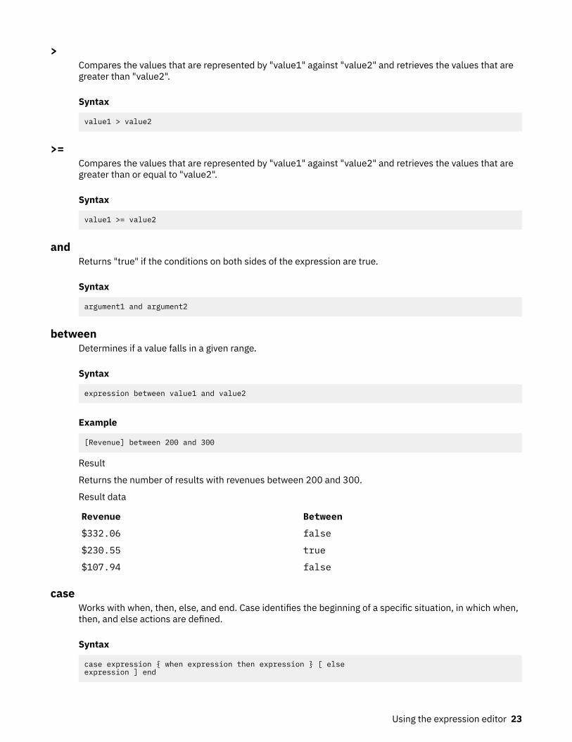
betweenDetermines if a value falls in a given range.

Syntax

expression between value1 and value2

Example

[Revenue] between 200 and 300

Result

Returns the number of results with revenues between 200 and 300.

Result data

Revenue Between

$332.06 false

$230.55 true

$107.94 false

caseWorks with when, then, else, and end. Case identifies the beginning of a specific situation, in which when,then, and else actions are defined.

Syntax

case expression { when expression then expression } [ else expression ] end

Using the expression editor 23

containsDetermines if "string1" contains "string2".

Syntax

string1 contains string2

distinctA keyword used in an aggregate expression to include only distinct occurrences of values. See also thefunction unique.

Syntax

distinct dataItem

Example

count ( distinct [OrderDetailQuantity] )

Result

1704

elseWorks with the if or case constructs. If the if condition or the case expression are not true, then the elseexpression is used.

Syntax

if ( condition ) then .... else ( expression ) , or case .... else ( expression ) end

endIndicates the end of a case or when construct.

Syntax

case .... end

ends withDetermines if "string1" ends with "string2".

Syntax

string1 ends with string2

ifWorks with the then and else constructs. If defines a condition; when the if condition is true, the thenexpression is used. When the if condition is not true, the else expression is used.

Syntax

if ( condition ) then ( expression ) else ( expression )


inDetermines if "expression1" exists in a given list of expressions.

Syntax

expression1 in ( expression_list )

is missingDetermines if "value" is undefined in the data.

Syntax

value is missing

likeDetermines if "string1" matches the pattern of "string2", with the character "char" optionally used toescape characters in the pattern string.

Syntax

string1 LIKE string2 [ ESCAPE char ]

Example 1

[PRODUCT_LINE] like 'G%'

Result

All product lines that start with 'G'.

Example 2

[PRODUCT_LINE] like '%Ga%' escape 'a'

Result

All the product lines that end with 'G%'.

lookupFinds and replaces data with a value you specify. It is preferable to use the case construct.

Syntax

lookup ( name ) in ( value1 --> value2 ) default ( expression )

Example

lookup ( [Country]) in ( 'Canada'--> ( [List Price] * 0.60), 'Australia'--> ( [List Price] * 0.80 ) ) default ( [List Price] )


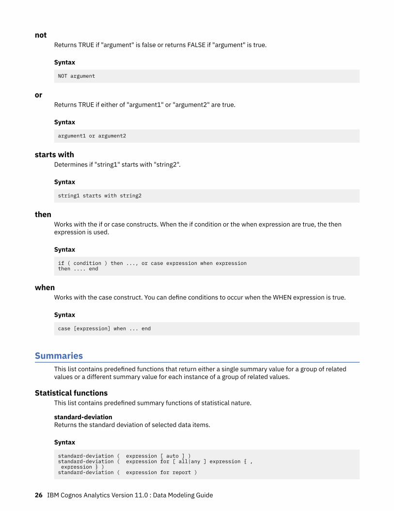
notReturns TRUE if "argument" is false or returns FALSE if "argument" is true.

Syntax

NOT argument

orReturns TRUE if either of "argument1" or "argument2" are true.

Syntax

argument1 or argument2

starts withDetermines if "string1" starts with "string2".

Syntax

string1 starts with string2

thenWorks with the if or case constructs. When the if condition or the when expression are true, the thenexpression is used.

Syntax

if ( condition ) then ..., or case expression when expression then .... end

whenWorks with the case construct. You can define conditions to occur when the WHEN expression is true.

Syntax

case [expression] when ... end

SummariesThis list contains predefined functions that return either a single summary value for a group of relatedvalues or a different summary value for each instance of a group of related values.

Statistical functionsThis list contains predefined summary functions of statistical nature.

standard-deviationReturns the standard deviation of selected data items.

Syntax

standard-deviation ( expression [ auto ] )standard-deviation ( expression for [ all|any ] expression { , expression } )standard-deviation ( expression for report )


Example

standard-deviation ( ProductCost )

Result

Returns a value indicating the deviation between product costs and the average product cost.

varianceReturns the variance of selected data items.

Syntax

variance ( expression [ auto ] )variance ( expression for [ all|any ] expression { , expression } )variance ( expression for report )

Example

variance ( Product Cost )

Result

Returns a value indicating how widely product costs vary from the average product cost.

averageReturns the average value of selected data items. Distinct is an alternative expression that is compatiblewith earlier versions of the product.

Syntax

average ( [ distinct ] expression [ auto ] )average ( [ distinct ] expression for [ all|any ] expression { , expression } )average ( [ distinct ] expression for report )

Example

average ( Sales )

Result

Returns the average of all Sales values.

countReturns the number of selected data items excluding null values. Distinct is an alternative expression thatis compatible with earlier versions of the product. All is supported in DQM mode only and it avoids thepresumption of double counting a data item of a dimension table.

Syntax

count ( [ all | distinct ] expression [ auto ] )count ( [ all | distinct ] expression for [ all|any ] expression { , expression } )count ( [ all | distinct ] expression for report )

Example

count ( Sales )

Result


Returns the total number of entries under Sales.

maximumReturns the maximum value of selected data items. Distinct is an alternative expression that iscompatible with earlier versions of the product.

Syntax

maximum ( [ distinct ] expression [ auto ] )maximum ( [ distinct ] expression for [ all|any ] expression { , expression } )maximum ( [ distinct ] expression for report )

Example

maximum ( Sales )

Result

Returns the maximum value out of all Sales values.

medianReturns the median value of selected data items.

Syntax

median ( expression [ auto ] )median ( expression for [ all|any ] expression { , expression } )median ( expression for report )

minimumReturns the minimum value of selected data items. Distinct is an alternative expression that is compatiblewith earlier versions of the product.

Syntax

minimum ( [ distinct ] expression [ auto ] )minimum ( [ distinct ] expression for [ all|any ] expression { , expression } )minimum ( [ distinct ] expression for report )

Example

minimum ( Sales )

Result

Returns the minimum value out of all Sales values.

percentageReturns the percent of the total value for selected data items. The "<for-option>" defines the scope of thefunction. The "at" option defines the level of aggregation and can be used only in the context of relationaldatasources.

Syntax

percentage ( numeric_expression [ at expression { , expression } ] [ <for-option> ] [ prefilter ] )


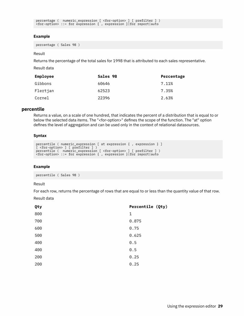
percentage ( numeric_expression [ <for-option> ] [ prefilter ] )<for-option> ::= for expression { , expression }|for report|auto

Example

percentage ( Sales 98 )

Result

Returns the percentage of the total sales for 1998 that is attributed to each sales representative.

Result data

Employee Sales 98 Percentage

Gibbons 60646 7.11%

Flertjan 62523 7.35%

Cornel 22396 2.63%

percentileReturns a value, on a scale of one hundred, that indicates the percent of a distribution that is equal to orbelow the selected data items. The "<for-option>" defines the scope of the function. The "at" optiondefines the level of aggregation and can be used only in the context of relational datasources.

Syntax

percentile ( numeric_expression [ at expression { , expression } ] [ <for-option> ] [ prefilter ] )percentile ( numeric_expression [ <for-option> ] [ prefilter ] )<for-option> ::= for expression { , expression }|for report|auto

Example

percentile ( Sales 98 )

Result

For each row, returns the percentage of rows that are equal to or less than the quantity value of that row.

Result data

Qty Percentile (Qty)

800 1

700 0.875

600 0.75

500 0.625

400 0.5

400 0.5

200 0.25

200 0.25


quantileReturns the rank of a value within a range that you specify. It returns integers to represent any range ofranks, such as 1 (highest) to 100 (lowest). The "<for-option>" defines the scope of the function. The "at"option defines the level of aggregation and can be used only in the context of relational datasources.

Syntax

quantile ( numeric_expression , numeric_expression [ at expression { , expression } ] [ <for-option> ] [ prefilter ] )quantile ( numeric_expression , numeric_expression [ <for-option> ] [ prefilter ] )<for-option> ::= for expression { , expression }|for report|auto

Example

quantile ( Qty , 4 )

Result

Returns the quantity, the rank of the quantity value, and the quantity values broken down into 4 quantilegroups (quartiles).

Result data

Qty Rank Quantile (Qty, 4)

800 1 1

700 2 1

600 3 2

500 4 2

400 5 3

400 5 3

200 7 4

200 7 4

quartileReturns the rank of a value, represented as integers from 1 (highest) to 4 (lowest), relative to a group ofvalues. The "<for-option>" defines the scope of the function. The "at" option defines the level ofaggregation and can be used only in the context of relational datasources.

Syntax

quartile ( numeric_expression [ at expression { , expression } ] [ <for-option> ] [ prefilter ] )quartile ( numeric_expression [ <for-option> ] [ prefilter ] )<for-option> ::= for expression { , expression }|for report|auto

Example

quartile ( Qty )

Result

Returns the quantity and the quartile of the quantity value represented as integers from 1 (highest) to 4(lowest).

Result data


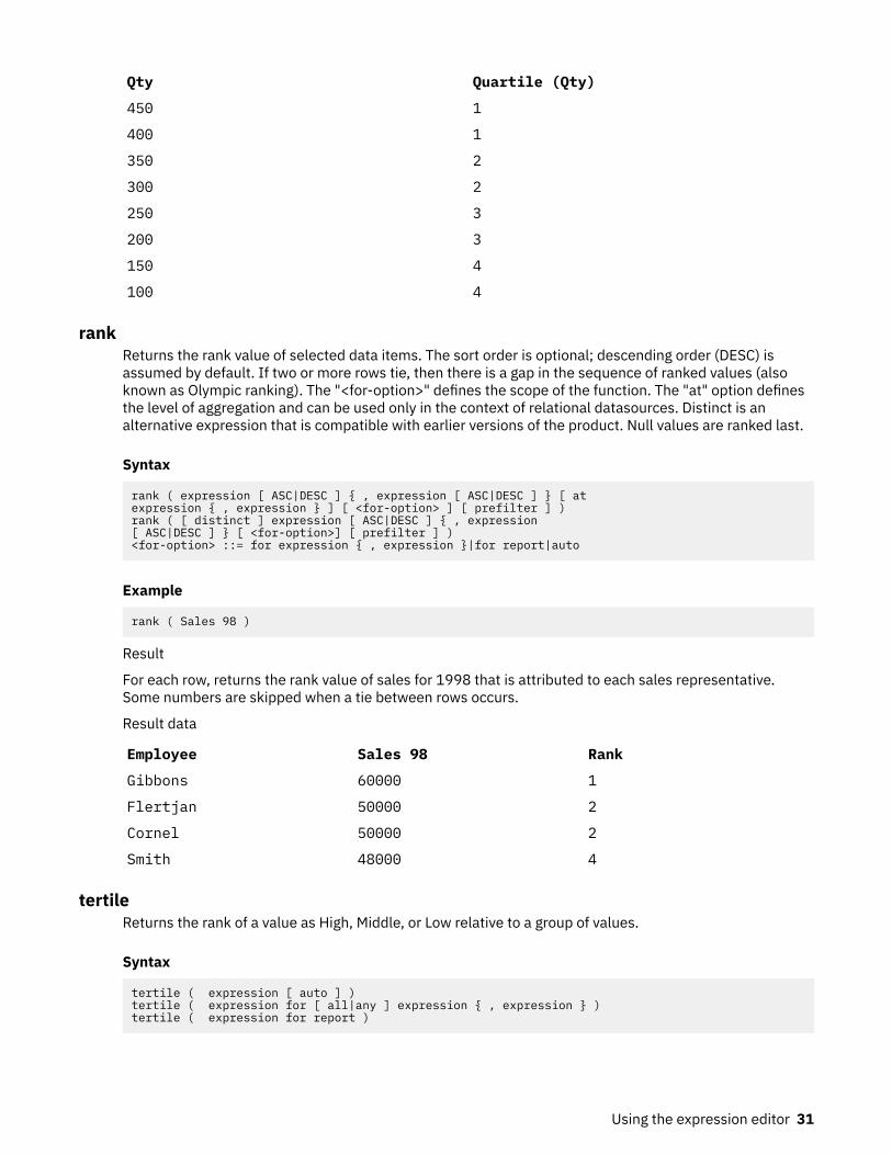
Qty Quartile (Qty)

450 1

400 1

350 2

300 2

250 3

200 3

150 4

100 4

rankReturns the rank value of selected data items. The sort order is optional; descending order (DESC) isassumed by default. If two or more rows tie, then there is a gap in the sequence of ranked values (alsoknown as Olympic ranking). The "<for-option>" defines the scope of the function. The "at" option definesthe level of aggregation and can be used only in the context of relational datasources. Distinct is analternative expression that is compatible with earlier versions of the product. Null values are ranked last.

Syntax

rank ( expression [ ASC|DESC ] { , expression [ ASC|DESC ] } [ at expression { , expression } ] [ <for-option> ] [ prefilter ] )rank ( [ distinct ] expression [ ASC|DESC ] { , expression [ ASC|DESC ] } [ <for-option>] [ prefilter ] )<for-option> ::= for expression { , expression }|for report|auto

Example

rank ( Sales 98 )

Result

For each row, returns the rank value of sales for 1998 that is attributed to each sales representative.Some numbers are skipped when a tie between rows occurs.

Result data

Employee Sales 98 Rank

Gibbons 60000 1

Flertjan 50000 2

Cornel 50000 2

Smith 48000 4

tertileReturns the rank of a value as High, Middle, or Low relative to a group of values.

Syntax

tertile ( expression [ auto ] )tertile ( expression for [ all|any ] expression { , expression } )tertile ( expression for report )


Example

tertile ( Qty )

Result

Returns the quantity, the quantile rank value of the quantity as broken down into tertiles, and the quantilerank label as broken down into tertiles.

Result data

Qty Quantile (Qty, 3) Tertile (Qty)

800 1 H

700 1 H

500 2 M

400 2 M

200 3 L

200 3 L

totalReturns the total value of selected data items. Distinct is an alternative expression that is compatible withearlier versions of the product.

Syntax

total ( [ distinct ] expression [ auto ] )total ( [ distinct ] expression for [ all|any ] expression { , expression } )total ( [ distinct ] expression for report )

Example

total ( Sales )

Result

Returns the total value of all Sales values.

Business Date/Time FunctionsThis list contains business functions for performing date and time calculations.

_add_secondsReturns the time or datetime, depending on the format of "time_expression", that results from adding"integer_expression" seconds to "time_expression".

Syntax

_add_seconds ( time_expression, integer_expression )

Example 1

_add_seconds ( 13:04:59 , 1 )

Result


13:05:00

Example 2

_add_seconds ( 2002-04-30 12:10:10.000, 1 )

Result

2002-04-30 12:10:11.000

Example 3

_add_seconds ( 2002-04-30 00:00:00.000, 1/100 )Note that the second argument is not a whole number. This is supported by some database technologies and increments the time portion.

Result

2002-04-30 00:00:00.010

_add_minutesReturns the time or datetime, depending on the format of "time_expression", that results from adding"integer_expression" minutes to "time_expression".

Syntax

_add_minutes ( time_expression, integer_expression )

Example 1

_add_minutes ( 13:59:00 , 1 )

Result

14:00:00

Example 2

_add_minutes ( 2002-04-30 12:59:10.000, 1 )

Result

2002-04-30 13:00:10.000

Example 3

_add_minutes ( 2002-04-30 00:00:00.000, 1/60 )Note that the second argument is not a whole number. This is supported by some database technologies and increments the time portion.

Result

2002-04-30 00:00:01.000


_add_hoursReturns the time or datetime, depending on the format of "time_expression", that results from adding"integer_expression" hours to "time_expression".

Syntax

_add_hours ( time_expression, integer_expression )

Example 1

_add_hours ( 13:59:00 , 1 )

Result

14:59:00

Example 2

_add_hours ( 2002-04-30 12:10:10.000, 1 )

Result

2002-04-30 13:10:10.000,

Example 3

_add_hours ( 2002-04-30 00:00:00.000, 1/60 )Note that the second argument is not a whole number. This is supported by some database technologies and increments the time portion.

Result

2002-04-30 00:01:00.000

_add_daysReturns the date or datetime, depending on the format of "date_expression", that results from adding"integer_expression" days to "date_expression".

Syntax

_add_days ( date_expression, integer_expression )

Example 1

_add_days ( 2002-04-30 , 1 )

Result

2002-05-01

Example 2

_add_days ( 2002-04-30 12:10:10.000, 1 )

Result

2002-05-01 12:10:10.000


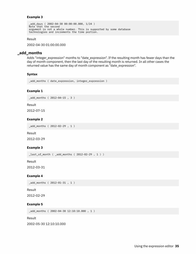
Example 3

_add_days ( 2002-04-30 00:00:00.000, 1/24 )Note that the second argument is not a whole number. This is supported by some database technologies and increments the time portion.

Result

2002-04-30 01:00:00.000

_add_monthsAdds "integer_expression" months to "date_expression". If the resulting month has fewer days than theday of month component, then the last day of the resulting month is returned. In all other cases thereturned value has the same day of month component as "date_expression".

Syntax

_add_months ( date_expression, integer_expression )

Example 1

_add_months ( 2012-04-15 , 3 )

Result

2012-07-15

Example 2

_add_months ( 2012-02-29 , 1 )

Result

2012-03-29

Example 3

_last_of_month ( _add_months ( 2012-02-29 , 1 ) )

Result

2012-03-31

Example 4

_add_months ( 2012-01-31 , 1 )

Result

2012-02-29

Example 5

_add_months ( 2002-04-30 12:10:10.000 , 1 )

Result

2002-05-30 12:10:10.000


_add_yearsAdds "integer_expression" years to "date_expression". If the "date_expression" is February 29 andresulting year is non leap year, then the resulting day is set to February 28. In all other cases the returnedvalue has the same day and month as "date_expression".

Syntax

_add_years ( date_expression, integer_expression )

Example 1

_add_years ( 2012-04-15 , 1 )

Result

2013-04-15

Example 2

_add_years ( 2012-02-29 , 1 )

Result

2013-02-28

Example 3

_add_years ( 2002-04-30 12:10:10.000 , 1 )

Result

2003-04-30 12:10:10.000

_ageReturns a number that is obtained from subtracting "date_expression" from today's date. The returnedvalue has the form YYYYMMDD, where YYYY represents the number of years, MM represents the numberof months, and DD represents the number of days.

Syntax

_age ( date_expression )

Example

_age ( 1990-04-30 ) (if today's date is 2003-02-05)

Result

120906, meaning 12 years, 9 months, and 6 days.

current_dateReturns a date value representing the current date of the computer that the database software runs on.

Syntax

current_date


Example

current_date

Result

2003-03-04

current_timeReturns a time with time zone value, representing the current time of the computer that runs the databasesoftware if the database supports this function. Otherwise, it represents the current time of the IBMCognos Analytics server.

Syntax

current_time

Example

current_time

Result

16:33:11.354+05:00

current_timestampReturns a datetime with time zone value, representing the current time of the computer that runs thedatabase software if the database supports this function. Otherwise, it represents the current time of theserver.

Syntax

current_timestamp

Example

current_timestamp

Result

2003-03-03 16:40:15.535+05:00

_day_of_weekReturns the day of week (1 to 7), where 1 is the first day of the week as indicated by the secondparameter (1 to 7, 1 being Monday and 7 being Sunday). Note that in ISO 8601 standard, a week beginswith Monday being day 1.

Syntax

_day_of_week ( date_expression, integer )

Example

_day_of_week ( 2003-01-01 , 1 )

Result

3


_day_of_yearReturns the day of year (1 to 366) in "date_ expression". Also known as Julian day.

Syntax

_day_of_year ( date_expression )

Example

_day_of_year ( 2003-03-01 )

Result

61

_days_betweenReturns a positive or negative number representing the number of days between "date_expression1" and"date_expression2". If "date_expression1" < "date_expression2", then the result will be a negativenumber.

Syntax

_days_between ( date_expression1 , date_expression2 )

Example

_days_between ( 2002-04-30 , 2002-06-21 )

Result

-52

_days_to_end_of_monthReturns a number representing the number of days remaining in the month represented by"date_expression".

Syntax

_days_to_end_of_month ( date_expression )

Example

_days_to_end_of_month ( 2002-04-20 14:30:22.123 )

Result

10

_end_of_dayReturns the end of today as a timestamp.

Syntax

_end_of_day


Example

_end_of_day

Result

2014-11-23 23:59:59

_first_of_monthReturns a date or datetime, depending on the argument, by converting "date_expression" to a date withthe same year and month but with the day set to 1.

Syntax

_first_of_month ( date_expression )

Example 1

_first_of_month ( 2002-04-20 )

Result

2002-04-01

Example 2

_first_of_month ( 2002-04-20 12:10:10.000 )

Result

2002-04-01 12:10:10.000

_from_unixtimeReturns the unix time specified by an integer expression as a timestamp with time zone.

Syntax

_from_unixtime ( integer_expression )

Example

_from_unixtime ( 1417807335 )

Result

2014-12-05 19:22:15+00:00

_hourReturns the value of the hour field in a date expression.

Syntax

_hour( date_expression )


Example

_hour ( 2002-01-31 12:10:10.254 )

Result

12

_last_of_monthReturns a date or datetime, depending on the argument, that is the last day of the month represented by"date_expression".

Syntax

_last_of_month ( date_expression )

Example 1

_last_of_month ( 2002-01-14 )

Result

2002-01-31

Example 2

_last_of_month ( 2002-01-14 12:10:10.000 )

Result

2002-01-31 12:10:10.000

_make_timestampReturns a timestamp constructed from "integer_expression1" (the year), "integer_expression2" (themonth), and "integer_expression3" (the day). The time portion defaults to 00:00:00.000 .

Syntax

_make_timestamp ( integer_expression1, integer_expression2, integer_expression3 )

Example

_make_timestamp ( 2002 , 01 , 14 )

Result

2002-01-14 00:00:00.000

_minuteReturns the value of the minute field in a date expression.

Syntax

_minute( date_expression )


Example

_minute ( 2002-01-31 12:10:10.254 )

Result

10

_monthReturns the value of the month field in a date expression.

Syntax

_month( date_expression )

Example

_month ( 2003-03-01 )

Result

3

_months_betweenReturns a positive or negative integer number representing the number of months between"date_expression1" and "date_expression2". If "date_expression1" is earlier than "date_expression2",then a negative number is returned.

Syntax

_months_between ( date_expression1, date_expression2 )

Example

_months_between ( 2002-04-03 , 2002-01-30 )

Result

2

_secondReturns the value of the second field in a date expression.

Syntax

_second( date_expression )

Example

_second ( 2002-01-31 12:10:10.254 )

Result

10.254


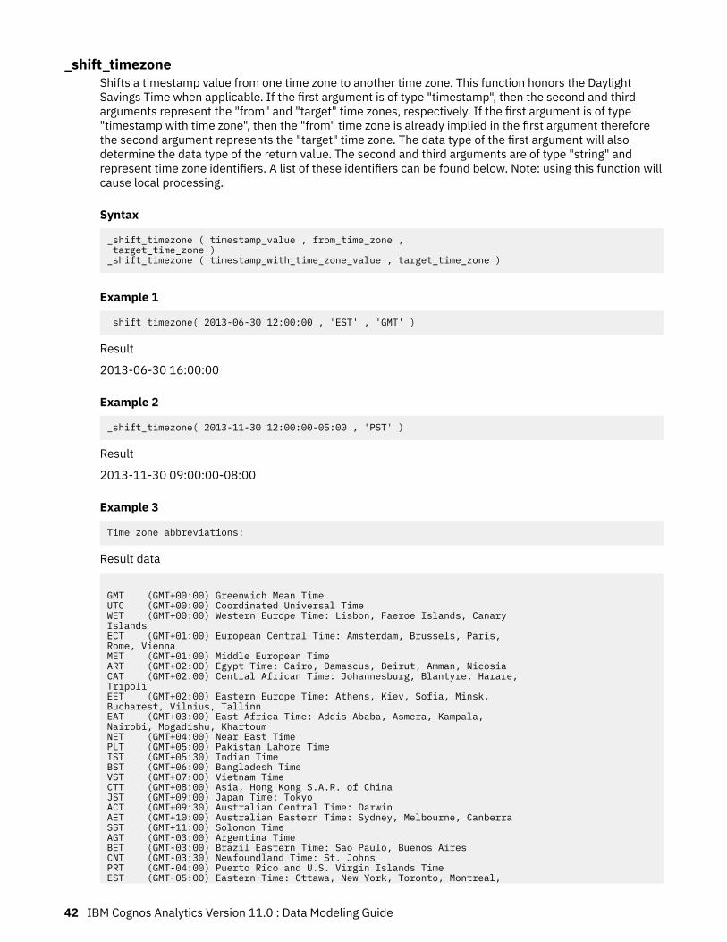
_shift_timezoneShifts a timestamp value from one time zone to another time zone. This function honors the DaylightSavings Time when applicable. If the first argument is of type "timestamp", then the second and thirdarguments represent the "from" and "target" time zones, respectively. If the first argument is of type"timestamp with time zone", then the "from" time zone is already implied in the first argument thereforethe second argument represents the "target" time zone. The data type of the first argument will alsodetermine the data type of the return value. The second and third arguments are of type "string" andrepresent time zone identifiers. A list of these identifiers can be found below. Note: using this function willcause local processing.

Syntax

_shift_timezone ( timestamp_value , from_time_zone , target_time_zone )_shift_timezone ( timestamp_with_time_zone_value , target_time_zone )

Example 1

_shift_timezone( 2013-06-30 12:00:00 , 'EST' , 'GMT' )

Result

2013-06-30 16:00:00

Example 2

_shift_timezone( 2013-11-30 12:00:00-05:00 , 'PST' )

Result

2013-11-30 09:00:00-08:00

Example 3

Time zone abbreviations:

Result data

GMT (GMT+00:00) Greenwich Mean TimeUTC (GMT+00:00) Coordinated Universal TimeWET (GMT+00:00) Western Europe Time: Lisbon, Faeroe Islands, Canary IslandsECT (GMT+01:00) European Central Time: Amsterdam, Brussels, Paris, Rome, ViennaMET (GMT+01:00) Middle European TimeART (GMT+02:00) Egypt Time: Cairo, Damascus, Beirut, Amman, NicosiaCAT (GMT+02:00) Central African Time: Johannesburg, Blantyre, Harare, TripoliEET (GMT+02:00) Eastern Europe Time: Athens, Kiev, Sofia, Minsk, Bucharest, Vilnius, TallinnEAT (GMT+03:00) East Africa Time: Addis Ababa, Asmera, Kampala, Nairobi, Mogadishu, KhartoumNET (GMT+04:00) Near East TimePLT (GMT+05:00) Pakistan Lahore TimeIST (GMT+05:30) Indian TimeBST (GMT+06:00) Bangladesh TimeVST (GMT+07:00) Vietnam TimeCTT (GMT+08:00) Asia, Hong Kong S.A.R. of ChinaJST (GMT+09:00) Japan Time: TokyoACT (GMT+09:30) Australian Central Time: DarwinAET (GMT+10:00) Australian Eastern Time: Sydney, Melbourne, CanberraSST (GMT+11:00) Solomon TimeAGT (GMT-03:00) Argentina TimeBET (GMT-03:00) Brazil Eastern Time: Sao Paulo, Buenos AiresCNT (GMT-03:30) Newfoundland Time: St. JohnsPRT (GMT-04:00) Puerto Rico and U.S. Virgin Islands TimeEST (GMT-05:00) Eastern Time: Ottawa, New York, Toronto, Montreal,


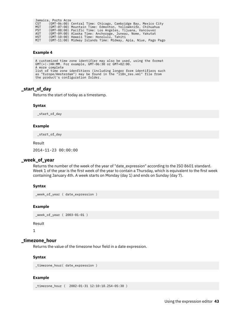
Jamaica, Porto AcreCST (GMT-06:00) Central Time: Chicago, Cambridge Bay, Mexico CityMST (GMT-07:00) Mountain Time: Edmonton, Yellowknife, ChihuahuaPST (GMT-08:00) Pacific Time: Los Angeles, Tijuana, VancouverAST (GMT-09:00) Alaska Time: Anchorage, Juneau, Nome, YakutatHST (GMT-10:00) Hawaii Time: Honolulu, TahitiMIT (GMT-11:00) Midway Islands Time: Midway, Apia, Niue, Pago Pago

Example 4

A customized time zone identifier may also be used, using the format GMT(+|-)HH:MM. For example, GMT-06:30 or GMT+02:00.A more complete list of time zone idenfitiers (including longer form identifiers such as "Europe/Amsterdam") may be found in the "i18n_res.xml" file from the product's configuration folder.

_start_of_dayReturns the start of today as a timestamp.

Syntax

_start_of_day

Example

_start_of_day

Result

2014-11-23 00:00:00

_week_of_yearReturns the number of the week of the year of "date_expression" according to the ISO 8601 standard.Week 1 of the year is the first week of the year to contain a Thursday, which is equivalent to the first weekcontaining January 4th. A week starts on Monday (day 1) and ends on Sunday (day 7).

Syntax

_week_of_year ( date_expression )

Example

_week_of_year ( 2003-01-01 )

Result

1

_timezone_hourReturns the value of the timezone hour field in a date expression.

Syntax

_timezone_hour( date_expression )

Example

_timezone_hour ( 2002-01-31 12:10:10.254-05:30 )


Result

5

_timezone_minuteReturns the value of the timezone minute field in a date expression.

Syntax

_timezone_minute( date_expression )

Example

_timezone_minute ( 2002-01-31 12:10:10.254-05:30 )

Result

30

_unix_timestampReturns the unix time specified by an integer expression as a timestamp with time zone.

Syntax

_unix_timestamp

Example

_unix_timestamp

Result

1416718800

_yearReturns the value of the year field in a date expression.

Syntax

_year( date_expression )

Example

_year ( 2003-03-01 )

Result

2003


_years_betweenReturns a positive or negative integer number representing the number of years between"date_expression1" and "date_expression2". If "date_expression1" < "date_expression2" then a negativevalue is returned.

Syntax

_years_between ( date_expression1, date_expression2 )

Example

_years_between ( 2003-01-30 , 2001-04-03 )

Result

1

_ymdint_betweenReturns a number representing the difference between "date_expression1" and "date_expression2". Thereturned value has the form YYYYMMDD, where YYYY represents the number of years, MM represents thenumber of months, and DD represents the number of days.

Syntax

_ymdint_between ( date_expression1 , date_expression2 )

Example

_ymdint_between ( 1990-04-30 , 2003-02-05 )

Result

120906, meaning 12 years, 9 months and 6 days.

Common Functions

absReturns the absolute value of "numeric_expression". Negative values are returned as positive values.

Syntax

abs ( numeric_expression )

Example 1

abs ( 15 )

Result

15

Example 2

abs ( -15 )

Result


15

castConverts "expression" to a specified data type. Some data types allow for a length and precision to bespecified. Make sure that the target is of the appropriate type and size. The following can be used for"datatype_specification": character, varchar, char, numeric, decimal, integer, bigint, smallint, real, float,date, time, timestamp, time with time zone, timestamp with time zone, and interval. When type casting toan interval type, one of the following interval qualifiers must be specified: year, month, or year to monthfor the year-to-month interval datatype; day, hour, minute, second, day to hour, day to minute, day tosecond, hour to minute, hour to second, or minute to second for the day-to-second interval datatype.Notes: When you convert a value of type timestamp to type date, the time portion of the timestamp valueis ignored. When you convert a value of type timestamp to type time, the date portion of the timestamp isignored. When you convert a value of type date to type timestamp, the time components of the timestampare set to zero. When you convert a value of type time to type timestamp, the date component is set to thecurrent system date. It is invalid to convert one interval datatype to the other (for instance because thenumber of days in a month is variable). Note that you can specify the number of digits for the leadingqualifier only, i.e. YEAR(4) TO MONTH, DAY(5). Errors will be reported if the target type and size are notcompatible with the source type and size.

Syntax

cast ( expression , datatype_specification )

Example 1

cast ( '123' , integer )

Result

123

Example 2

cast ( 12345 , varchar ( 10 ) )

Result

a string containing 12345

ceilingReturns the smallest integer that is greater than or equal to "numeric_expression".

Syntax

ceiling ( numeric_expression )

Example 1

ceiling ( 4.22 )

Result

5

Example 2

ceiling ( -1.23 )


Result

-1

char_lengthReturns the number of logical characters in "string_expression". The number of logical characters can bedistinct from the number of bytes in some East Asian locales.

Syntax

char_length ( string_expression )

Example

char_length ( 'Canada' )

Result

6

coalesceReturns the first non-null argument (or null if all arguments are null). Requires two or more arguments in"expression_list".

Syntax

coalesce ( expression_list )

Example

coalesce ( [Unit price], [Unit sale price] )

Result

Returns the unit price, or the unit sale price if the unit price is null.

expReturns 'e' raised to the power of "numeric_expression". The constant 'e' is the base of the naturallogarithm.

Syntax

exp ( numeric_expression )

Example

exp ( 2 )

Result

7.389056


floorReturns the largest integer that is less than or equal to "numeric_expression".

Syntax

floor ( numeric_expression )

Example 1

floor ( 3.22 )

Result

3

Example 2

floor ( -1.23 )

Result

-2

lnReturns the natural logarithm of "numeric_expression".

Syntax

ln ( numeric_expression )

Example

ln ( 4 )

Result

1.38629

lowerReturns "string_expression" with all uppercase characters shifted to lowercase.

Syntax

lower ( string_expression )

Example

lower ( 'ABCDEF' )

Result

abcdef


modReturns the remainder (modulus) of "integer_expression1" divided by "integer_expression2"."Integer_expression2" must not be zero or an exception condition is raised.

Syntax

mod ( integer_expression1, integer_expression2 )

Example

mod ( 20 , 3 )

Result

2

nullifReturns null if "expression1" equals "expression2", otherwise returns "expression1".

Syntax

nullif ( expression1, expression2 )

positionReturns the integer value representing the starting position of "string_expression1" in"string_expression2" or 0 when the "string_expression1" is not found.

Syntax

position ( string_expression1 , string_expression2 )

Example 1

position ( 'C' , 'ABCDEF' )

Result

3

Example 2

position ( 'H' , 'ABCDEF' )

Result

0

position_regexReturns the integer value representing the beginning or ending position of the substring in"string_expression" that matches the regular expression "regex_expression". The search starts at position"integer_expression1", which has a default value of 1. The occurrence of the pattern to search for isspecified by "integer_expression2", which has a default value of 1. The return option, specified by the firstargument, specifies what is returned in relation to the occurrence. If you specify "start", the position ofthe first character of the occurrence is returned. If you specify "after", the position of the characterfollowing the occurrence is returned. If you don't specify a return option, "start" is implicit. Flags to setoptions for the interpretation of the regular expression are specified by "flags_expression". Individualletters are used to define the flags, with valid values being 's', 'm', 'i', and 'x'.


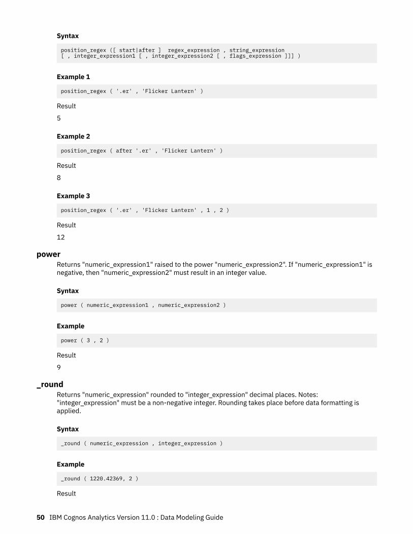
Syntax

position_regex ([ start|after ] regex_expression , string_expression[ , integer_expression1 [ , integer_expression2 [ , flags_expression ]]] )

Example 1

position_regex ( '.er' , 'Flicker Lantern' )

Result

5

Example 2

position_regex ( after '.er' , 'Flicker Lantern' )

Result

8

Example 3

position_regex ( '.er' , 'Flicker Lantern' , 1 , 2 )

Result

12

powerReturns "numeric_expression1" raised to the power "numeric_expression2". If "numeric_expression1" isnegative, then "numeric_expression2" must result in an integer value.

Syntax

power ( numeric_expression1 , numeric_expression2 )

Example

power ( 3 , 2 )

Result

9

_roundReturns "numeric_expression" rounded to "integer_expression" decimal places. Notes:"integer_expression" must be a non-negative integer. Rounding takes place before data formatting isapplied.

Syntax

_round ( numeric_expression , integer_expression )

Example

_round ( 1220.42369, 2 )

Result


1220.42

sqrtReturns the square root of "numeric_expression". "Numeric_expression" must be non-negative.

Syntax

sqrt ( numeric_expression )

Example

sqrt ( 9 )

Result

3

substringReturns the substring of "string_expression" that starts at position "integer_expression1" for"integer_expression2" characters or to the end of "string_expression" if "integer_expression2" is omitted.The first character in "string_expression" is at position 1.

Syntax

substring ( string_expression , integer_expression1 [ , integer_expression2 ] )

Example

substring ( 'abcdefg' , 3 , 2 )

Result

cd

substring_regexReturns a substring of "string_expression" that matches the regular expression "regex_expression". Thesearch starts at position "integer_expression1", which has a default value of 1. The occurrence of thepattern to search for is specified by "integer_expression2", which has a default value of 1. Flags to setoptions for the interpretation of the regular expression are specified by "flags_expression". Individualletters are used to define the flags, with valid values being 's', 'm', 'i', and 'x'.

Syntax

substring_regex ( regex_expression , string_expression [ , integer_expression1[ , integer_expression [ , flags_expression ]]] )

Example 1

substring_regex ( '.er' , 'Flicker Lantern')

Result

ker


Example 2

substring_regex ( '.er' , 'Flicker Lantern' , 1 , 2 )

Result

ter

trimReturns "string_expression" trimmed of leading and trailing blanks or trimmed of a certain characterspecified in "match_character_expression". "Both" is implicit when the first argument is not stated andblank is implicit when the second argument is not stated.

Syntax

trim ( [ [ trailing|leading|both ] [ match_character_expression ] , ] string_expression )

Example 1

trim ( trailing 'A' , 'ABCDEFA' )

Result

ABCDEF

Example 2

trim ( both , ' ABCDEF ' )

Result

ABCDEF

upperReturns "string_expression" with all lowercase characters converted to uppercase.

Syntax

upper ( string_expression )

Example

upper ( 'abcdef' )

Result

ABCDEF

Trigonometric functions

arccosReturns the arc cosine of the argument, where the argument is in the range of -1 to 1 and the result is avalue expressed in radians.

Syntax

arccos ( numeric_expression )


Example

arccos ( -1 )

Result

3.1415

arcsinReturns the arc sine of the argument, where the argument is in the range of -1 to 1 and the result is avalue expressed in radians.

Syntax

arcsin ( numeric_expression )

Example

arcsin ( 0 )

Result

3.1415

arctanReturns the arc tangent of the argument, where the argument is in the range of -1 to 1 and the result is avalue expressed in radians.

Syntax

arctan ( numeric_expression )

Example

arctan ( 0 )

Result

3.1415

cosReturns the cosine of the argument, where the argument is expressed in radians.

Syntax

cos ( numeric_expression )

Example

cos ( 0.3333 * 3.1415 )

Result

0.5


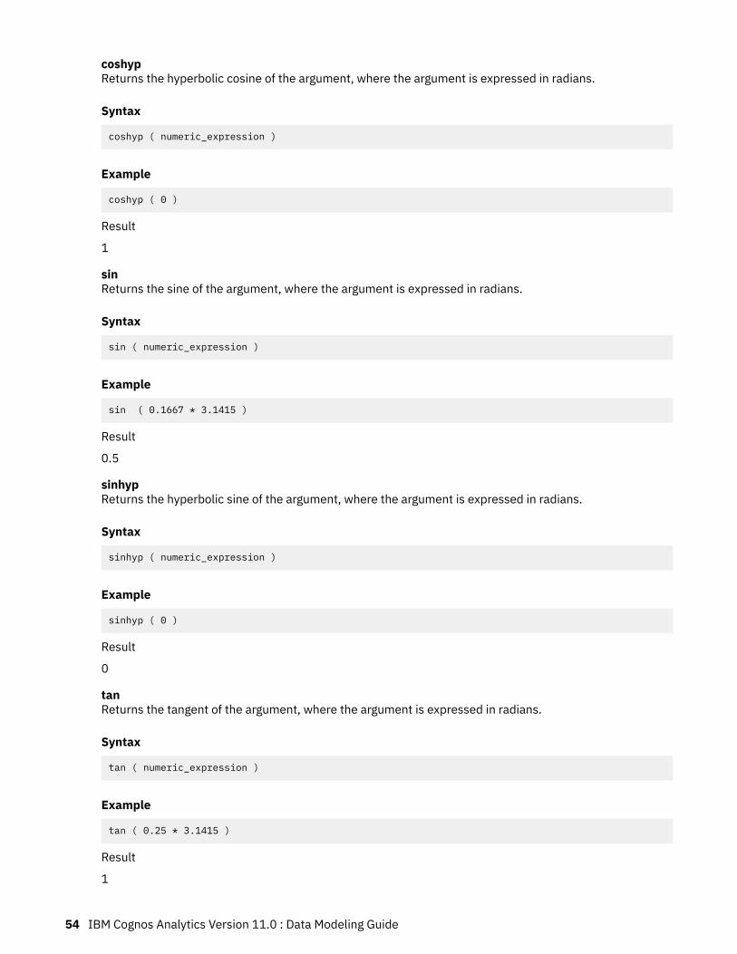
coshypReturns the hyperbolic cosine of the argument, where the argument is expressed in radians.

Syntax

coshyp ( numeric_expression )

Example

coshyp ( 0 )

Result

1

sinReturns the sine of the argument, where the argument is expressed in radians.

Syntax

sin ( numeric_expression )

Example

sin ( 0.1667 * 3.1415 )

Result

0.5

sinhypReturns the hyperbolic sine of the argument, where the argument is expressed in radians.

Syntax

sinhyp ( numeric_expression )

Example

sinhyp ( 0 )

Result

0

tanReturns the tangent of the argument, where the argument is expressed in radians.

Syntax

tan ( numeric_expression )

Example

tan ( 0.25 * 3.1415 )

Result

1


tanhypReturns the hyperbolic tangent of the argument, where the argument is expressed in radians.

Syntax

tanhyp ( numeric_expression )

Example

tanhyp ( 0 )

Result

0


Appendix B. About this guideThis document is intended for use with IBM Cognos Analytics. Cognos Analytics integrates reporting,modeling, analysis, dashboards, metrics, and event management so you can understand yourorganization's data, and make effective business decisions.

To find product documentation on the web, including all translated documentation, access IBMKnowledge Center (http://www.ibm.com/support/knowledgecenter).

Accessibility features

Accessibility features help users who have a physical disability, such as restricted mobility or limitedvision, to use information technology products successfully. For information on accessibility features inCognos Analytics, see the Cognos Analytics Accessibility Guide.

Forward-looking statements

This documentation describes the current functionality of the product. References to items that are notcurrently available may be included. No implication of any future availability should be inferred. Any suchreferences are not a commitment, promise, or legal obligation to deliver any material, code, orfunctionality. The development, release, and timing of features or functionality remain at the solediscretion of IBM.

Samples disclaimer

The Sample Outdoors Company, Great Outdoors Company, GO Sales, any variation of the SampleOutdoors or Great Outdoors names, and Planning Sample depict fictitious business operations withsample data used to develop sample applications for IBM and IBM customers. These fictitious recordsinclude sample data for sales transactions, product distribution, finance, and human resources. Anyresemblance to actual names, addresses, contact numbers, or transaction values is coincidental. Othersample files may contain fictional data manually or machine generated, factual data compiled fromacademic or public sources, or data used with permission of the copyright holder, for use as sample datato develop sample applications. Product names referenced may be the trademarks of their respectiveowners. Unauthorized duplication is prohibited.


http://www.ibm.com/support/knowledgecenter

http://www.ibm.com/support/knowledgecenter

Index

Aaggregate property 18

Ccleaning

columns in modules 13

Ddata modeling 1data modules

editing 9relinking sources 6table and column properties 18

Eediting data modules

undo and redo actions 9user interface 9

editing modulesvalidation errors 17

expression editorBusiness Date/Time Functions 32Common Functions 45Statistical functions 26Summaries 26Trigonometric functions 52

Ffilters

adding 16removing 16

Hhiding

tables and columns 17

Iidentifier property 18

Mmodeling user interface 9modules

cleaning data 13editing 13hiding tables and columns 17validating 17

Nnavigation path

creating 15deleting 15

Pproperties

tables and columns 18

Rredo

editing data modules 9relinking

sources in a data module 6

Ssources

relinking in a data module 6

Uundo

editing data modules 9usage property 18

Vvalidating

modules 17

59

Version 11.0 IBM Cognos Analytics€¦ · Chapter 1. Data modeling in Cognos Analytics ... cast ......

Documents

Transcript of Version 11.0 IBM Cognos Analytics€¦ · Chapter 1. Data modeling in Cognos Analytics ... cast ......