Verilog-A and Verilog-AMS Reference...
140
Verilog-A and Verilog-AMS Reference Manual September 2007
Transcript of Verilog-A and Verilog-AMS Reference...

Verilog-A and Verilog-AMSReference Manual
September 2007

NoticeThe information contained in this document is subject to change without notice.
Agilent Technologies makes no warranty of any kind with regard to this material, including, but not limited to, the implied warranties of merchantability and fitness for a particular purpose. Agilent Technologies shall not be liable for errors contained herein or for incidental or consequential damages in connection with the furnishing, perfor-mance, or use of this material.
Warranty
A copy of the specific warranty terms that apply to this software product is available upon request from your Agi-lent Technologies representative.
Restricted Rights Legend
Use, duplication or disclosure by the U. S. Government is subject to restrictions as set forth in subparagraph (c) (1) (ii) of the Rights in Technical Data and Computer Software clause at DFARS 252.227-7013 for DoD agencies, and subparagraphs (c) (1) and (c) (2) of the Commercial Computer Software Restricted Rights clause at FAR 52.227-19 for other agencies.
© Agilent Technologies, Inc. 1983-2007. 395 Page Mill Road, Palo Alto, CA 94304 U.S.A.
Acknowledgments
Mentor Graphics is a trademark of Mentor Graphics Corporation in the U.S. and other countries.
Microsoft®, Windows®, MS Windows®, Windows NT®, and MS-DOS® are U.S. registered trademarks of Microsoft Corporation.
Pentium® is a U.S. registered trademark of Intel Corporation.
PostScript® and Acrobat® are trademarks of Adobe Systems Incorporated.
UNIX® is a registered trademark of the Open Group.
Java™ is a U.S. trademark of Sun Microsystems, Inc.
SystemC® is a registered trademark of Open SystemC Initiative, Inc. in the United States and other countries and is used with permission.
MATLAB® is a U.S. registered trademark of The Math Works, Inc.
HiSIM2 source code, and all copyrights, trade secrets or other intellectual property rights in and to the source code in its entirety, is owned by Hiroshima University and STARC.
ii

Contents1 Overview and Benefits
Analog Modeling....................................................................................................... 1-1Hardware Description Languages ............................................................................ 1-1Verilog-A ................................................................................................................... 1-2Compact Models....................................................................................................... 1-2Simulation................................................................................................................. 1-4
2 Verilog-A/AMS ModulesDeclaring Modules.................................................................................................... 2-1
Module Instantiation ........................................................................................... 2-1Ports ......................................................................................................................... 2-2Describing Analog Behavior ..................................................................................... 2-2Branches .................................................................................................................. 2-3Analog Signals.......................................................................................................... 2-3
Accessing Net and Branch Signals .................................................................... 2-3User-defined Analog Functions ................................................................................ 2-4Hierarchical Structures ............................................................................................. 2-6
Module Instance Parameter Value Assignment.................................................. 2-6Port Assignment ................................................................................................. 2-7Scope ................................................................................................................. 2-8
3 Lexical ConventionsWhite Space ............................................................................................................. 3-2Comments ................................................................................................................ 3-2Operators.................................................................................................................. 3-2Strings ...................................................................................................................... 3-2Numbers ................................................................................................................... 3-3
Integer Numbers................................................................................................. 3-3Real Numbers .................................................................................................... 3-3Scale Factors...................................................................................................... 3-3
Keywords .................................................................................................................. 3-4Identifiers .................................................................................................................. 3-4System Tasks and Functions.................................................................................... 3-5Compiler Directives .................................................................................................. 3-5
4 Data TypesInteger ...................................................................................................................... 4-1Real .......................................................................................................................... 4-1Type Conversion ....................................................................................................... 4-1Net Discipline............................................................................................................ 4-2Ground Declaration .................................................................................................. 4-3
iii

Implicit Nets .............................................................................................................. 4-3Genvar ...................................................................................................................... 4-4Parameters ............................................................................................................... 4-4
5 Analog Block StatementsSequential Block....................................................................................................... 5-1Conditional Statement (if-else) ................................................................................. 5-1Case Statement........................................................................................................ 5-2Repeat Statement..................................................................................................... 5-3While Statement ....................................................................................................... 5-3For Statement........................................................................................................... 5-4
6 Mathematical Functions and OperatorsUnary/Binary/Ternary Operators .............................................................................. 6-1
Arithmetic Operators .......................................................................................... 6-2Relational Operators .......................................................................................... 6-2Logical Operators ............................................................................................... 6-3Bit-wise Operators .............................................................................................. 6-3Shift Operators ................................................................................................... 6-4Conditional (Ternary) Operator........................................................................... 6-4Precedence ........................................................................................................ 6-5Concatenation Operator ..................................................................................... 6-5Expression Evaluation ........................................................................................ 6-5Arithmetic Conversion ........................................................................................ 6-6
Mathematical Functions............................................................................................ 6-6Standard Mathematical Functions...................................................................... 6-6Transcendental Functions................................................................................... 6-7
Statistical Functions.................................................................................................. 6-8The $random Function ....................................................................................... 6-8The $dist_uniform and $rdist_uniform Functions ............................................... 6-9The $dist_normal and $rdist_normal Functions ................................................. 6-9The $dist_exponential and $rdist_exponential Functions................................... 6-10The $dist_poisson and $rdist_poisson Functions .............................................. 6-10The $dist_chi_square and $rdist_chi_square Functions .................................... 6-11The $dist_t and $rdist_t Functions ..................................................................... 6-11The $dist_erlang and $rdist_erlang Functions ................................................... 6-12
7 Analog Operators and FiltersTolerances ................................................................................................................ 7-1Parameters ............................................................................................................... 7-1Time Derivative Operator.......................................................................................... 7-2Time Integrator Operator .......................................................................................... 7-2Circular Integrator Operator...................................................................................... 7-3
iv
Absolute Delay Operator .......................................................................................... 7-3Transition Filter ......................................................................................................... 7-4Slew Filter................................................................................................................. 7-6Last Crossing Function............................................................................................. 7-7Limited Exponential .................................................................................................. 7-7Laplace Transform Filters ......................................................................................... 7-8
laplace_zp() ........................................................................................................ 7-8laplace_zd() ........................................................................................................ 7-9laplace_np()........................................................................................................ 7-10laplace_nd()........................................................................................................ 7-10
Z-Transform Filters ................................................................................................... 7-11zi_zp()................................................................................................................. 7-11zi_zd()................................................................................................................. 7-12zi_np() ................................................................................................................ 7-13zi_nd() ................................................................................................................ 7-14
8 Analog EventsGlobal Events ........................................................................................................... 8-1
The initial_step Event ......................................................................................... 8-1The final_step Event........................................................................................... 8-2Global Event Return Codes................................................................................ 8-2
Monitored Events...................................................................................................... 8-3The cross Function............................................................................................. 8-3The timer Function ............................................................................................. 8-4
Event or Operator ..................................................................................................... 8-5Event Triggered Statements ..................................................................................... 8-5
9 Mixed Signal Behavior ModelsIntroduction to AMS.................................................................................................. 9-1Describing Behavior for Analog and Digital Simulation ............................................ 9-2
Accessing Discrete Nets and Variables from a Continuous Context .................. 9-4Accessing X and Z Bits of a Discrete Net in a Continuous Context ................... 9-5Accessing Continuous Nets and Variables from a Discrete Context .................. 9-6Detecting Discrete Events in a Continuous Context ........................................... 9-6Detecting Continuous Events in a Discrete Context ........................................... 9-6Concurrency (Synchronization) .......................................................................... 9-7
Discipline Resolution ................................................................................................ 9-7Connect Modules...................................................................................................... 9-8
Driver-Receiver Segregation .............................................................................. 9-13
10 Verilog-A/AMS and the SimulatorEnvironment Parameter Functions ........................................................................... 10-1
The temperature Function .................................................................................. 10-1
v

The abstime Function......................................................................................... 10-1The realtime Function......................................................................................... 10-1The Thermal Voltage Function ........................................................................... 10-2
Controlling Simulator Actions ................................................................................... 10-2Bounding the Time Step..................................................................................... 10-2Announcing Discontinuities ................................................................................ 10-3
Analysis Dependent Functions ................................................................................. 10-3Analysis Function ............................................................................................... 10-3AC Stimulus Function ......................................................................................... 10-5Noise Functions.................................................................................................. 10-5
11 System Tasks and I/O FunctionsThe $param_given Function..................................................................................... 11-1The $table_model Function ...................................................................................... 11-2
Table Model Inputs ............................................................................................. 11-3Table Data Source .............................................................................................. 11-3Table Control String............................................................................................ 11-4
File Input/Output Operations .................................................................................... 11-7The $fopen Function........................................................................................... 11-7The $fclose Function .......................................................................................... 11-7The $fstrobe Function ........................................................................................ 11-8The $fdisplay Function ....................................................................................... 11-8The $fwrite Function........................................................................................... 11-9
Display Output Operations........................................................................................ 11-9The $strobe Function ......................................................................................... 11-9The $display Function ........................................................................................ 11-9Format Specification........................................................................................... 11-10
Simulator Control Operations ................................................................................... 11-11The $finish Simulator Control Operation ............................................................ 11-11The $stop Simulator Control Operation .............................................................. 11-11
12 The Verilog-A/AMS PreprocessorDefining Macros........................................................................................................ 12-1Including Files........................................................................................................... 12-2Conditional Compilation............................................................................................ 12-3Predefined Macros ................................................................................................... 12-4Verilog-AMS and Verilog 1364 1995/2001 Directives ............................................... 12-4Unsupported Directives ............................................................................................ 12-4
A Reserved Words in Verilog-A/AMS
B Unsupported Elements
C Standard DefinitionsThe disciplines.vams File.......................................................................................... C-1
vi

The constants.vams File........................................................................................... C-6The compact.vams File ............................................................................................ C-7
D Condensed ReferenceVerilog-A Module Template....................................................................................... D-1Data Types................................................................................................................ D-2Analog Operators and Filters.................................................................................... D-2Mathematical Functions............................................................................................ D-4Transcendental Functions......................................................................................... D-5AC Analysis Stimuli................................................................................................... D-5Noise Functions........................................................................................................ D-6Analog Events .......................................................................................................... D-6Timestep Control ...................................................................................................... D-7Input/Output Functions ............................................................................................. D-8Simulator Environment Functions............................................................................. D-8Module Hierarchy...................................................................................................... D-9
Index
vii

viii

Chapter 1: Overview and BenefitsThis chapter introduces the Verilog-A language and software in terms of its capabilities, benefits, and typical use.
Analog ModelingAnalog modeling enables designers to capture high-level behavioral descriptions of components in a precise set of mathematical terms. The analog module’s relation of input to output can be related by the external parameter description and the mathematical relations between the input and output ports.
Analog models give the designer control over the level of abstraction with which to describe the action of the component. This can provide higher levels of complexity to be simulated, allow faster simulation execution speeds, or can hide intellectual property.
An analog model should ideally model the characteristics of the behavior as accurately as possible, with the trade off being model complexity, which is usually manifested by reduced execution speed. For electrical models, besides the port relationship of charges and currents, the developer may need to take thermal behavior, physical layout considerations, environment (substrate, wires) interaction, noise, and light, among other things into consideration. Users prefer that the model be coupled to measurable quantities. This provides reassurance in validating the model, but also provides a means to predict future performance as the component is modified.
Models often have to work with controlling programs besides the traditional simulator. Optimization, statistical, reliability, and synthesis programs may require other information than which the model developer was expecting.
Hardware Description LanguagesHardware description languages (HDLs) were developed as a means to provide varying levels of abstraction to designers. Integrated circuits are too complex for an engineer to create by specifying the individual transistors and wires. HDLs allow the performance to be described at a high level and simulation synthesis programs can then take the language and generate the gate level description.
Analog Modeling 1-1

Overview and Benefits
Verilog and VHDL are the two dominant languages; this manual is concerned with the Verilog language.
As behavior beyond the digital performance was added, a mixed-signal language was created to manage the interaction between digital and analog signals. A subset of this, Verilog-A, was defined. Verilog-A describes analog behavior only; however, it has functionality to interface to some digital behavior.
Verilog-AVerilog-A provides a high-level language to describe the analog behavior of conservative systems. The disciplines and natures of the Verilog-A language enable designers to reflect the potential and flow descriptions of electrical, mechanical, thermal, and other systems.
Verilog-A is a procedural language, with constructs similar to C and other languages. It provides simple constructs to describe the model behavior to the simulator program. The model effectively de-couples the description of the model from the simulator.
The model creator provides the constitutive relationship of the inputs and outputs, the parameter names and ranges, while the Verilog-A compiler handles the necessary interactions between the model and the simulator. While the language does allow some knowledge of the simulator, most model descriptions should not need to know anything about the type of analysis being run.
Compact ModelsCompact models are the set of mathematical equations that describe the performance of a device. Commercial simulators use compact models to describe the performance of semiconductor devices, most typically transistors.
There is a wide range of modeling categories, including neural nets, empirical, physical, and table based. Each has distinct advantages and disadvantages as listed in Table 1-1 below.
1-2 Verilog-A

For electrical modeling, most compact device models use empirical modeling based on physical models. This provides the best combination of execution speed, accuracy, and prediction. However, non-physical behavior may result when the equations are used outside their fitting range. Model creators should also be aware of the issues around parameter extraction. If a model’s parameters cannot easily or accurately be extracted, the model will not be successful.
Once created, a compact model can be implemented in a simulator in a variety of methods (see Table 1-2). Each method has its own advantages and disadvantages, but in general, the simpler the interface, the less capable it is.
Table 1-1. Modeling Categories
Type Advantage Disadvantage
Physical Predicts performance bestExtrapolates
Must understand physicsSlow
Empirical Reasonably good predictionFast
Can give non-physical behavior
Tabular Very generalEasy to extractReasonable execution speed
Cannot extrapolateMinimal parameter info
Neural net Very generalReasonable execution speed
Cannot extrapolateMinimal parameter info
Table 1-2. Compact Model Simulator Implementation Methods
Type Advantage Disadvantage
Macro model Simple, portable Limited to available primitives
Proprietary interface Power, fast Need access to simulatorNot portable
Compact Models 1-3

Overview and Benefits
The most powerful interface is the proprietary interface to the simulator. For many reasons, most typically intellectual property protection, the proprietary interface is not made public. This is because the interface usually requires such intimate details of the simulator analysis operation that a clever investigator could discern much detail about the inner workings of the simulation algorithms.
On the other hand, a detailed, complex interface also requires a detailed understanding by the model developer to properly access the functionality of the analysis. This can require as much effort as the development of the model itself. If the model is to be added using this interface to other simulators, often the effort of learning one interface does not provide much advantage in learning the nuances of the other.
Simulator vendors often provide simplified interfaces, either a scaled-back code level interface, or a custom symbolic interface. The simplicity always comes at a price of reduced functionality, decreased execution speed, or a lack of portability.
Analog Hardware Description languages (AHDLs) solve most of these problems, except the problem of execution speed. However, compiler technology in Advanced Design System provides the abstraction and simplicity of Verilog-A with an execution speed with a factor of two of code level interfaces.
SimulationMost analog simulators evolved from the SPICE program released by UC Berkeley. The analog simulator solves a simple set of relations for a large number of unknowns to provide the designer with the voltage and currents at each of the nodes in the circuit as either a function of time or frequency. The electrical relations are simply the Kirchoff current law and voltage loop laws:
Public interface Reasonably powerful Usually missing some capabilityNot portableUnique complexitySlow
AHDLs (Verilog-A) SimplePowerPortableProtected
Language has some restrictions
Table 1-2. Compact Model Simulator Implementation Methods
Type Advantage Disadvantage
1-4 Simulation

• The instantaneous currents from all branches entering a node must sum to zero.
• The instantaneous voltages around any closed loop must sum to zero.
Figure 1-1. Kirchoff ’s Current and Voltage Laws.
The program solves these equations using an algorithm known as Newton-Raphson. The program guesses a solution to the relation:
F(v,t)=0
It next calculates if the solution is close enough, and if it is, it stops. If the program needs to find the next guess, it calculates the Jacobian of the function (the set of partial derivatives), which provides a pointer towards the real solution. This is best seen in a simple case where F(v,t) is one dimensional:
I1 V1I2
I3
V2V4
V3
+ -
+
+
+
-
-
-
Simulation 1-5

Overview and Benefits
Figure 1-2. Newton-Raphson Algorithm where r is the root.
The program calculates F(x1) and then uses the derivative (the slope of the line) to estimate the zero-crossing. It then uses this new point, x2, as the next guess. As long as the function is continuous and smooth (and the program does not get stuck in local minima), the program will quickly approach, or converge to, the actual point where F(X) crosses zero.
In modern simulation programs the trick is to quickly find the solution for a large number of variables, and for variables that may have strong (nonlinear) relations to independent variables.
During a simulation, the program queries each element in the circuit for information. The resistor, the capacitor, or the transistor, for example, needs to report back to the simulator its behavior at a particular guess. It must also report back its slope with respect to the voltages at that point.
The behavior of each element is described by mathematical equations that, taken as a group, are called a compact device model. The compact device model can be very simple or very complicated. For example, in the simplest case, a resistor can be described by Ohm’s law:
I = V/R
The derivative is a constant, the inverse of the resistance.
However, even for simple components like resistors, the models can become rather complicated when other effects are added, such as, self-heating, self-inductance,
x1x2
guess 1
guess 2
F(x)
x
r
1-6 Simulation

thermal noise, etc. The Verilog-A compiler manages all of the necessary interfaces so that, for the most part, the developer need only be concerned with model behavior.
Simulation 1-7

Overview and Benefits
1-8 Simulation

Chapter 2: Verilog-A/AMS ModulesThis chapter discusses the concept of Verilog-A modules. The chapter shows the basic structure of a module declaration, how to define parameters and ports, and how to define a simple analog block.
Declaring ModulesThe module declaration provides the simulator with the name of the module, the input and output ports, parameter information, and the behavioral description of the model. Top-level modules are modules which are included in the source text but are not instantiated. Module definitions cannot contain the text of another module definition. A module definition can nest another module by instantiating it. For more information, refer to “Hierarchical Structures” on page 2-6.
Module Instantiation
Syntax
module | macromodule module_identifier [(port {, port, ...})]module_statements
endmodule
where module_identifier is the name of the module and the optional list of port name(s) defines the connections to the module, and module_statements describe the module behavior.
Example
The simplest example is a resistor.
‘include "disciplines.vams"module R(p,n);
electrical p,n;parameter real R=50.0;analog
V(p,n) <+ R * I(p,n);endmodule
The first line provides common definitions. The line module R(p, n); declares the module name to be R and that it has 2 ports, named p and n, which the next line further describes by attributing the electrical discipline to the ports.
Declaring Modules 2-1

Verilog-A/AMS Modules
This module has one parameter, R, which is declared as a real type with a default value of 50.0. Parameters provide a way to pass information into the module at the time of instantiation.
The analog block, in this example a single line, describes the behavior using a voltage contribution statement to assign the voltage based on the access function value of I() times R.
PortsPorts provide a way to connect modules to other modules and devices. A port has a direction: input, output, or inout, which must be declared. The ports are listed after the module declaration. The port type and port direction must then be declared in the body of the module.
Examples
module resistor(p,n);inout p,n;electrical p,n;
…
module modName(outPort, inPort);output outPort;input inPort;electrical outPort, inPort;
…
Ports can support vectors (buses) as well.
Describing Analog BehaviorThe analog behavior of the component is described with procedural statements defined within an analog block. During simulation, all of the analog blocks are evaluated. Each module is evaluated in the design as though it were contributing concurrently to the analysis.
Syntax
analog block_statement
where block_statement is a single analog statement of a group of statements.
2-2 Ports

Examples
analog V(n1, n2) <+ 1; // A simple 1 volt source
analog begin // A multi-statement analog blockvin = V(in);if (vin >= signal_in_dead_high)
vout = vin - signal_in_dead_high;else
if (vin <= signal_in_dead_low)vout = vin - signal_in_dead_low;
elsevout = 0.0;
V(out) <+ vout;end
BranchesA branch is defined as a path between two nets. A branch is conservative if both nets are conservative and two associated quantities, potential and flow, are defined for the branch. If either net is a signal-flow net, then the branch is defined as a signal-flow branch with either a potential or flow defined for the branch.
Syntax
branch list_of_branches
where list_of_branches is a comma-separated list of branch names.
Analog SignalsAnalog signals are signals associated with a discipline that has a continuous domain. Their value can be accessed and set via various functions and contribution statements. This section describes the analog signal functions. It describes how to access signal data from nodes and vectors, as well as how to use the contribution operator.
Accessing Net and Branch Signals
Signals on nets and branches can be accessed only by the access functions of the associated discipline. The name of the net or the branch is specified as the argument to the access function.
Branches 2-3

Verilog-A/AMS Modules
Examples
Vin = V(in);CurrentThruBranch = I(myBranch);
Indirect branch assignment
An indirect branch assignment is useful when it is difficult to solve an equation. It has this format,
V(n) : V(p) == 0;
which can be read as “find V(n) such that V(p) is equal to zero.” This example shows that node n should be driven with a voltage source and the voltage should be such that the given equation is satisfied. V(p) is probed and not driven.
Note Indirect branch assignments are allowed only within the analog block.
Branch Contribution Statement
A branch contribution statement typically consists of a left-hand side and a right-hand side, separated by a branch contribution operator. The right-hand side can be any expression which evaluates to (or can be promoted to) a real value. The left-hand side specifies the source branch signal to assign the right-hand side. It consists of a signal access function applied to a branch. The form is,
V(n1, n2) <+ expression;
I(n1, n2) <+ expression;
Branch contribution statements implicitly define source branch relations. The branch extends from the first net of the access function to the second net. If the second net is not specified in the call, the global reference node (ground) is used as the reference net.
User-defined Analog FunctionsAnalog functions provide a modular way for a user-defined function to accept parameters and return a value. The functions are defined as analog or digital and must be defined within modules blocks.
The analog function is of the form:
2-4 User-defined Analog Functions

analog function {real|integer} function_name;input_declaration;statement_block;
endfunction
The input_declaration describes the input parameters to the function as well as any variables used in the statement block:
input passed_parameters;real parameter_list;
The statement_block and analog function:
• can use any statements available for conditional execution
• cannot use access functions
• cannot use contribution statements or event control statements
• must have at least one input declared; the block item declaration declares the type of the inputs as well as local variables used
• cannot use named blocks
• can only reference locally-defined variables or passed variable arguments
The analog function implicitly declares a variable of the same name as the function, function_name. This variable must be assigned in the statement block; its last assigned value is passed back.
Example
analog function real B_of_T;input B, T, T_NOM, XTB;real B, T, T_NOM, XTB;begin
B_of_T = B * pow(T / T_NOM, XTB);end
endfunction
The function is called by the line,
BF_T = B_of_T(BF, T, T_NOM, XTB);
User-defined Analog Functions 2-5

Verilog-A/AMS Modules
Hierarchical StructuresVerilog-A supports hierarchical descriptions, whereby modules can instantiate other modules. This section describes the procedure for implementing and calling hierarchical models.
Syntax
module_or_primative [#(.param1(expr)[, .param2(expr))]]instance_name
({node {, node});
Examples
phaseDetector #(.gain(2)) pd1(lo, rf, if_);
vco #(.gain(loopGain/2), .fc(fc) ) vco1(out, lo);
Module Instance Parameter Value Assignment
The default parameter values can be overridden by assigning them via an ordered list or explicitly when instantiating a module.
By Order
In this method, the assignment order in the instance declaration follows the order of the parameter declaration in the module declaration. It is not necessary to assign all of the parameters, but all parameters to the left of a declaration must be defined (that is, parameters to the left of the last declaration can not be skipped).
Example
// Voltage Controlled Oscillatormodule vco(in, out); inout in, out;electrical in, out;parameter real gain = 1, fc = 1;analog
V(out) <+ sin(2*‘M_PI*(fc*$realtime() + idt(gain*V(in))));endmodule...
// Instantiate a vco module name vco1 connected to out and // lo with gain = 0.5, fc = 2kvco #(0.5, 2000.0) vco1(out, lo);
2-6 Hierarchical Structures

By Name
Alternatively, instance parameters can be assigned explicitly by their name, where the name matches the parameter name in the module. In this method, only the parameters that are modified from their default values need to be assigned.
Example
// Voltage Controlled Oscillator
module vco(in, out); inout in, out;electrical in, out;parameter real gain = 1, fc = 1;analog
V(out) <+ sin(2*‘M_PI*(fc*$realtime() + idt(gain*V(in))));
endmodule
...
// Instantiate a vco module name vco1 connected to out and lo with // gain = loopGain/2, fc = fc
vco #(.gain(loopGain/2), .fc(fc) ) vco1(out, lo);
Port Assignment
Ports can be assigned either via an ordered list or directly by name.
By Order
To connect ports by an ordered list, the ports in the instance declaration should be listed in the same order as the module port definition.
Example
module sinev(n1,n2);electrical n1,n2;parameter real gain = 1.0, freq = 1.0;analog begin
V(n2,n1) <+ gain * sin(2 * ‘M_PI * freq * $abstime);$bound_step(0.05/freq);
endendmodule...
Hierarchical Structures 2-7

Verilog-A/AMS Modules
// Instantiate a source1 with in->n1, out->n2sinev #(.gain(G), .freq(F) ) source1(in, out)
Scope
Verilog-A supports name spaces for the following elements:
• modules
• tasks
• named blocks
• functions
• analog functions
Within each scope only one identifier can be declared. To reference an identifier directly, the identifier must be declared locally in the named block, or within a module, or within a named block that is higher in the same branch of the name hierarchy that contains the named block. If an identifier is declared locally, it will be used, otherwise the identifier will be searched upwards until it is found, or until a module boundary is reached.
2-8 Hierarchical Structures

Chapter 3: Lexical ConventionsThis chapter describes the overall lexical conventions of Verilog-A, and how the language defines and interprets various elements such as white space, strings, numbers, and keywords.
Verilog-A consists of lexical tokens (one or more characters) of the form:
• “White Space” on page 3-2
• “Comments” on page 3-2
• “Operators” on page 3-2
• “Strings” on page 3-2
• “Numbers” on page 3-3
• “Keywords” on page 3-4
• “Identifiers” on page 3-4
• “System Tasks and Functions” on page 3-5
• “Compiler Directives” on page 3-5
The source file is free form where spaces, tabs, and newlines are only token separators and have no other significance. Lines can be extended using the line continuation character / where needed.
3-1

Lexical Conventions
White SpaceWhite space consists of spaces, tabs, newlines, and form feeds. They separate tokens, otherwise are ignored.
CommentsThere are two ways to include comments:
• A single line comment starts with // and continues to the end of the line.
Example
// This is a single line comment
• Block statements begin with /* and end with */ and cannot be nested but can include single line comments.
Example
/* This is a block comment which can include any ASCII character
*/
OperatorsVerilog-A has unary (single) operators, binary (double) operators and the conditional operator. Unary operators appear to the left of the operand, and binary between their operands. The conditional operator separates the three operands with two special characters.
StringsStrings are sequences of characters enclosed by double quotes and contained on one line.
Example
"This is a string."
3-2 White Space

NumbersConstant numbers can be specified as integer or a real constants; complex constants are not allowed. Scale factors can be used for readability on real numbers.
Integer Numbers
Integer constants must be specified as a sequence of the digits 0 through 9 in a decimal format with an optional + or - unary operator at the start. The underscore character can be used at any position except the first character as a means to break up the number for readability.
Examples
12345
-122
867_5309
Real Numbers
Real constants follow the IEEE standard for double precision floating point numbers, IEEE STD-754-1985. They can be specified in decimal notation or scientific notation. If a decimal point is used, the number must have at least one digit on each side of the decimal point (e.g., 0.1 or 17.0 are allowed, .1 or 17. are not). As in the integer case, the underscore character is allowed anywhere but the first character and is ignored.
Examples
3.14
1.23e-9
27E9
876_763_300E10
Scale Factors
Scale factors can be used on floating point numbers, but cannot be used with numbers in scientific format. The scale factor symbol and the number cannot have a space between them.
Numbers 3-3

Lexical Conventions
Examples
KeywordsKeywords are predefined non-escaped identifiers. Keywords define the language constructs. They are defined in lowercase only. Appendix A, Reserved Words in Verilog-A/AMS, lists all of the keywords, which includes the Verilog-AMS keywords.
IdentifiersIdentifiers give objects unique names for reference and can consist of any sequence of letters, digits, the $ character, and the _ (underscore) character. The first character of an identifier can be a letter or underscore, it cannot be the $ character or a digit. Identifiers are case sensitive.
Table 3-1. Scale Factors
Scale Factor Symbol Multiplier
T 1012
G 109
M 106
K or k 103
m 10-3
µ 10-6
n 10-9
p 10-12
f 10-15
a 10-18
2.5m 2.5e-3 0.025
0.11M 1.1e5 110000
3-4 Keywords

Examples
deviceName
i
Vth0
vth0
_device
sheet_rho$
System Tasks and FunctionsUser-defined tasks and functions use a $ character to declare a system task or system function. Any valid identifier, including keywords (not already in use in this construct), can be used as system task and system function names. Note that for backward compatibility with earlier versions of Verilog-A, this implementation reserves some task and function names.
Examples
$temperature;
$strobe(“hello”);
Compiler DirectivesCompiler directives are indicated using the ` (accent grave) character. For more information, refer to Chapter 12, The Verilog-A/AMS Preprocessor, for a discussion of compiler directives.
System Tasks and Functions 3-5

Lexical Conventions
3-6 Compiler Directives

Chapter 4: Data TypesThis section describes the various data types that Verilog-A supports as well as shows the correct format and use model. Verilog-A supports integer, real, parameter, and discipline data types.
IntegerAn integer declaration declares one or more variables of type integer holding values ranging from -231 to 231-1. Arrays of integers can be declared using a range which defines the upper and lower indices of the array where the indices are constant expressions and shall evaluate to a positive or negative integer, or zero.
Example
integer flag, MyCount, I[0:63];
RealA real declaration declares one or more variables of type real using IEEE STD-754-1985 (the IEEE standard for double precision floating point numbers). Arrays of reals can be declared using a range which defines the upper and lower indices of the array where the indices are constant expressions and shall evaluate to a positive or negative integer, or zero.
Example
real X[1:10], Tox, Xj, Cgs;
Type ConversionVerilog-A maintains the number type during expression evaluation and will also silently convert numbers to the type of the variable. This can lead to unexpected behavior. For example, the contribution statement,
I(di,si) <+ white_noise(4 * ‘P_K * T * (2/3) * abs(gm), "shot");
will always return 0 since the 2/3 term is evaluated using integer mathematics, and no noise is contributed from the noise power expression. Instead, use 2.0/3.0 which will evaluate to a real number.
Integer 4-1

Data Types
Net DisciplineThe net discipline is used to declare analog nets. A net is characterized by the discipline that it follows. Because a net is declared as a type of discipline, a discipline can be considered as a user-defined type for declaring a net.
A discipline is a set of one or more nature definitions forming the definition of an analog signal whereas a nature defines the characteristics of the quantities for the simulator. A discipline is characterized by the domain and the attributes defined in the natures for potential and flow.
The discipline can bind:
• One nature with potential
• Nothing with either potential or flow (an empty discipline)
System defined disciplines are predefined in the disciplines.vams file, a portion of which is shown below.
// Electrical
// Current in amperesnature Currentunits = "A";access = I;idt_nature = Charge;`ifdef CURRENT_ABSTOL
abstol = `CURRENT_ABSTOL;`else
abstol = 1e-12;`endifendnature
// Charge in coulombsnature Chargeunits = "coul";access = Q;ddt_nature = Current;`ifdef CHARGE_ABSTOL
abstol = `CHARGE_ABSTOL;`else
abstol = 1e-14;`endifendnature
// Potential in voltsnature Voltageunits = "V";
4-2 Net Discipline

access = V;idt_nature = Flux;`ifdef VOLTAGE_ABSTOL
abstol = `VOLTAGE_ABSTOL;`else
abstol = 1e-6;`endifendnature
Ground DeclarationA global reference node, or ground, can be associated with an already declared net of continuous discipline.
Syntax
ground list_of_nets;
where list_of_nets is a comma-separated list of nets.
Example
`include “disciplines.vams”module load(p);
electrical p, gnd;ground gnd;parameter real R=50.0;analog
V(p) <+ R * I(p, gnd);endmodule
Implicit NetsNets used in a structural description do not have to be explicitly declared. The net is declared implicitly as scalar, the discipline as empty, and the domain as undefined.
Example
`include “disciplines.vams”module Implicit_ex(Input1, Input2, Output1, Output2, Output3);input Input1, Input2;output Output1, Output2, Output3;electrical Input1, Input2, Output1, Output2, Output3;blk_a a1(Input1, a_b1);blk_a a2(Input2, a_b2);blk_b b1(a_b1, c_b1);
Ground Declaration 4-3

Data Types
blk_b b2 (a_b2, c_b2);blk_c c1(Output1,Output2, Output3,c_b1,c_b2);
endmodule
GenvarGenvars are used for accessing analog signals within behavioral looping constructs.
genvar list_of_genvar_identifiers;
where list_of_genvar_identifiers is a comma-separated list of genvar identifiers.
Example
genvar i, j;
ParametersParameters provide the method to bring information from the circuit to the model.
Parameter assignments are a comma-separated list of assignments. The right hand side of the assignment is a constant expression (including previously defined parameters).
For parameter arrays, the initializer is a list of constant expressions containing only constant numbers and previously defined parameters within bracket delimiters, { }.
Parameter values cannot be modified at runtime.
parameter {real | integer} list_of_assignments;
where the list_of_assignments is a comma separated list of
parameter_identifier = constant [value-range]
where value-range is of the form
from value_range_specifier| exclude value_range_specifier| exclude constant_expression
where the value_range_specifier is of the form
start_paren expression1 : expression2 end_paren
where start_paren is “[“ or “(“ and end_paren is “]” or “)” and expression1 is constant_expression or “-inf“ and expression2 is constant_expression or “inf”.
4-4 Genvar

The type (real | integer) is optional. If it is not given, it will be derived from the constant assignment value. A parenthesis indicates the range can go up to, but not include the value, whereas a bracket indicates the range includes the endpoint. Value ranges can have simple exclusions as well.
Examples
/* Define a parameter of type real with a default value of 0 and allowed values between 0 and up to, but not including, infinity and excluding values between 10 and 100 (however, 10 and 100 are acceptable) and 200 and 400 (200 is acceptable, but 400 is not.) */parameter real TestFlag = 0 from [0:inf) exclude (10:100) exclude (200:400];
/* Define a real parameter with a default value of 27, ranging from -273.15 up to, but not including infinity. */parameter real Temp = 27 from [-273.15:inf);
/* Define a parameter R with a default value of 50, ranging from, but not including, 0 to infinity. R is implicitly defined as type integer. */parameter R = 50 from (0:inf];
Parameters 4-5

Data Types
4-6 Parameters

Chapter 5: Analog Block StatementsThis chapter describes the analog block. The analog block is where most of the analog behavior is described. This chapter will discuss the various procedural control statements available in Verilog-A.
Sequential BlockA sequential block is a grouping of two or more statements into one single statement.
Syntax
begin [ : block_identifier [ block_item_declaration ]]{ statement }end
The optional block identifier allows for naming of the block. Named blocks allow local variable declaration.
Example
if (Vds < 0.0) begin: RevModereal T0; // T0 is visible in this block onlyT0 = Vsb;Vsb = Vsb + Vds;Vdss = - Vds + T0;
end
Conditional Statement (if-else)The conditional statement is used to determine whether a statement is executed or not.
Syntax
if ( expression ) true_statement;[ else false_statement; ]
If the expression evaluates to true (non-zero), then the true_statement will be executed. If there is an else false_statement and the expression evaluates to false (zero), the false_statement is executed instead.
Conditional statements may be nested to any level.
Sequential Block 5-1

Analog Block Statements
Example
if (Vd < 0)begin
if (Vd < -Bv)Id = -Area * Is_temp * (limexp(-(Bv + Vd) / Vth) + Bv / Vth);
else if (Vd == -Bv)Id = -Area * Ibv_calc;
else if (Vd <= -5 * N * Vth)Id = -Area * Is_temp;
else // -5 nKT/q <= Vd < 0Id = Area * Is_temp * (limexp(Vd / Vth) - 1);
endelse
Id = Area * Is_temp * (limexp(Vd / (N * Vth)) - 1);
Case StatementA case statement is useful where multiple actions can be selected based on an expression. The format is:
case ( expression ) case_item { case_item } endcase
where case_item is:
expression { , expression } : statement_or_null| default [ : ] statement_or_null
The default-statement is optional; however, if it is used, it can only be used once. The case expression and the case_item expression can be computed at runtime (neither expression is required to be a constant expression). The case_item expressions are evaluated and compared in the exact order in which they are given. If one of the case_item expressions matches the case expression given in parentheses, then the statement associated with that case_item is executed. If all comparisons fail then the default item statement is executed (if given). Otherwise none of the case_item statements are executed.
5-2 Case Statement

Example
case(rgeo)1, 2, 5: begin
if (nuEnd == 0.0)Rend = 0.0;
elseRend = Rsh * DMCG / (Weffcj * nuEnd);
end3, 4, 6: begin
if ((DMCG + DMCI) == 0.0)$strobe("(DMCG + DMCI) cannot be equal to zero\n");
if (nuEnd == 0.0)Rend = 0.0;
elseRend = Rsh * Weffcj / (3.0 * nuEnd * (DMCG + DMCI));
enddefault:
$strobe("Warning: Specified RGEO = %d not matched (BSIM4RdsEndIso)\n", rgeo);endcase
Repeat StatementThe repeat() statement executes a statement a fixed number of times. The number is given by the repeat expression.
Syntax
repeat ( expression ) statement
Example
repeat (devIndex - startIndex) begindevTemp = incrByOne(devTemp, offset);
end
While Statementwhile() executes a statement until its control expression becomes false. If the expression is false when the loop is entered, the statement is not executed at all.
Syntax
while ( expression ) statement
Repeat Statement 5-3

Analog Block Statements
Example
while(devTemp < T) begindevTemp = incrTemp(devTemp, offset);
end
For StatementThe for() statement controls execution of its associated statement(s) using an index variable. If the associated statement is an analog statement, then the control mechanism must consist of genvar assignments and genvar expressions only. No use of procedural assignments and expressions are allowed.
Syntax
for ( procedural_assignment ; expression;procedural_assignment ) statement
If the for() loop contains an analog statement, the format is:
for ( genvar_assignment; genvar_expression;genvar_assignment ) analog_statement
Note that the two are syntactically equivalent except that the executed statement is also an analog statement (with the associated restrictions).
Example
for (i = 0; i < maxIndex; i = i +1;) beginoutReg[i] = getValue(i);
end
5-4 For Statement

Chapter 6: Mathematical Functions and OperatorsVerilog-A supports a range of functions and operators that may be used to form expressions that describe model behavior and to control analog procedural block flow. Return values from these functions are only a function of the current parameter value.
Unary/Binary/Ternary OperatorsArithmetic operators follow conventions close to the C programming language.
Table 6-1. Unary/Binary/Ternary Operators
Operator Type
+ - * / Arithmetic
% Modulus
> >= < <= Relational
!= == Logical equality
! Logical negation
&& Logical and
|| Logical or
~ Bit-wise negation
& Bit-wise and
| Bit-wise inclusive or
^ Bit-wise exclusive or
^~ ~^ Bit-wise equivalence
<< Left shift
>> Right shift
?: Conditional
or Event or
{} {{ }} Concatenation, replication
Unary/Binary/Ternary Operators 6-1

Mathematical Functions and Operators
Arithmetic Operators
The arithmetic operators are summarized in Table 6-2.
See also “Precedence” on page 6-5 and “Arithmetic Conversion” on page 6-6.
Relational Operators
Table 6-3 defines and summarizes the relational operators.
The relational operators evaluate to a zero (0) if the relation is false or one (1) if the relation evaluates to true. Arithmetic operations are performed before relational operations.
Examples
a = 10;b = 0;a < b evaluates to false.
Table 6-2. Arithmetic operators
Operator Function
a + b a plus b
a - b a minus b
a * b a times b
a / b a divided by b
a % b a modulo b
Table 6-3. Relational operators
Operator Function
a < b a is less than b
a > b a is greater than b
a <= b a is less than or equal to b
a >= b a is greater than or equal to b
6-2 Unary/Binary/Ternary Operators

Logical Operators
Logical operators consist of equality operators and connective operators and are summarized in Table 6-4.
Bit-wise Operators
Bit-wise operators perform operations on the individual bits of the operands following the logic described in the tables below.
Table 6-4. Logical operators
Operator Function
a == b a is equal to b
a != b a is not equal to b
a && b a AND b
a || b a OR b
!a not a
Table 6-5. Bitwise and operator
& 0 1
0 0 0
1 0 1
Table 6-6. Bitwise or operator
| 0 1
0 0 1
1 1 1
Table 6-7. Bitwise exclusive or operator
^ 0 1
0 0 1
1 1 0
Unary/Binary/Ternary Operators 6-3

Mathematical Functions and Operators
Shift Operators
The shift operators shift their left operand either right (>>) or left (<<) by the number of bit positions indicated by their right operand, filling the vacated bit positions with zeros (0). The right operand is treated as an unsigned number.
Example
integer mask, new;analog begin
mask = 1;new = (mask << 4);
end
Conditional (Ternary) Operator
The conditional operator consists of three operands, separated by the operators ? (question mark) and : (colon).
Syntax
expression1 ? expression2 : expression3
The expression1 is first evaluated. If it evaluates to false (0) then expression3 is evaluated and becomes the result. If expression1 is true (any non-zero value), then expression2 is evaluated and becomes the result.
Example
BSIM3vth0 = (BSIM3type == ‘NMOS) ? 0.7 : -0.7;
Table 6-8. Bitwise exclusive nor operator
^~~^ 0 1
0 1 0
1 0 1
Table 6-9. Bitwise negation operator
~
0 1
1 1
6-4 Unary/Binary/Ternary Operators

Precedence
Table 6-10 shows the precedence order of the operators, with operators in the same row having equal precedence. Association is left to right with the exception of the conditional (ternary) operator, which associates right to left. Parentheses can be used to control the order of the evaluation.
Concatenation Operator
The concatenation operator {} is used for joining scalar elements into compound elements.
Example
parameter real taps[0:3] = {1.0, 2.0, 3.0, 4.0};
Expression Evaluation
The expression evaluation follows the order precedence described in Table 6-10. If the results of an expression can be determined without evaluating the entire expression, the remaining part of the expression is not evaluated, unless it contains analog expressions. This expression evaluation rule is known as short-circuiting.
Table 6-10. Precedence
Operators Priority
+ - ! ~ (unary) Highest
* / % ..
+ - (binary) ..
<< >> ..
== != ..
& ~& ..
^ ^~ ~^ ..
| ~| ..
&& ..
|| ..
? : Lowest
Unary/Binary/Ternary Operators 6-5

Mathematical Functions and Operators
Arithmetic Conversion
Verilog-A performs automatic conversion of numeric types based on the operation. For functions that take integers, real numbers are converted to integers by rounding to the nearest integer, with ties rounded away from zero (0). For operators, a common data type is determined based on the operands. If either operand is real, the other operand is converted to real.
Examples
a = 7.0 + 3; // 3 becomes 3.0 and then the addition is performed, a = 10.0
a = 1 / 3; // The result of this integer division is zero, a = 0.
a = 7.0 + 1 / 3; /* The 1/3 is evaluated by integer division, cast to 0.0 and added to 7.0, a = 7.0; */
Mathematical FunctionsVerilog-A supports a wide range of functions to help in describing analog behavior. These include the standard mathematical functions, transcendental and hyperbolic functions, and a set of statistical functions.
Standard Mathematical Functions
The mathematical functions supported by Verilog-A are shown in Table 6-11.
Table 6-11. Mathematical Functions Supported by Verilog-A
Function Description Domain Return value
ln() natural log x>0 real
log(x) log base 10 x>0 real
exp(x) exponential X<80 real
sqrt(x) square root x>=0 real
min(x,y) minimum of x and y all x, y if either is real, returns real, otherwise returns the type of x,y.
max(x,y) maximum of x and y all x, y if either is real, returns real, otherwise returns the type of x,y.
abs(x) absolute value all x same as x
6-6 Mathematical Functions

For the min(), max(), and abs() functions, the derivative behavior is defined as:
min(x,y) is equivalent to (x < y) ? x : y
max(x,y) is equivalent to (x >y) ? x : y
abs(x) is equivalent to (x > 0) ? x : -x
Transcendental Functions
The transcendental functions supported by Verilog-A are shown in Table 6-12. All operands are integer or real and will be converted to real when necessary. The arguments to the trigonometric and hyperbolic functions are specified in radians.
The return values are real.
pow(x,y) xy if x>=0, all y;if x<0, int(y)
real
floor(x) floor all x real
ceil(x) ceiling all x real
Table 6-12. Transcendental Functions Supported by Verilog-A
Function Description Domain
sin(x) sine all x
cos(x) cosine all x
tan(x) tangent x != n (pi/2), n is odd
asin(x) arc-sine -1<= x <= 1
acos(x) arc-cosine -1<= x <= 1
atan(x) arc-tangent all x
atan2(x,y) arc-tangent of x/y all x, all y
hypot(x,y) sqrt(x2 + y2) all x, all y
sinh(x) hyperbolic sine x < 80
cosh(x) hyperbolic cosine x < 80
tanh(x) hyperbolic tangent all x
asinh(x) arc-hyperbolic sine all x
Table 6-11. Mathematical Functions Supported by Verilog-A
Function Description Domain Return value
Mathematical Functions 6-7

Mathematical Functions and Operators
Statistical FunctionsVerilog-A supports a variety of functions to provide statistical distributions. All parameters are real valued with the exception of seed_expression, an integer. The functions return a pseudo-random number, of type real, based on the distribution type. When a seed is passed to one of these functions, the seed is modified. The system functions return the same value for a given seed value.
The $random Function
The $random() function returns a new 32-bit random number each time it is called. The return type is a signed integer.
Note The modulus operator, %, can be used to restrict the return value.For b > 0, $random %b will restrict the random number to (-b+1) : (b-1).
Syntax
$random[( seed_expression )];
where
The optional seed_expression can be used to control the random number generation and must be a signed integer variable.
Example
integer seed_value, random_value;random_value = $random;// returns a value between -31 and 31.random_value = $random(seed_value) % 32;
acosh(x) arc-hyperbolic cosine x >= 1
atanh(x) arch-hyperbolic tangent -1 <= x <= 1
Table 6-12. Transcendental Functions Supported by Verilog-A
Function Description Domain
6-8 Statistical Functions

The $dist_uniform and $rdist_uniform Functions
The $dist_uniform() and $rdist_uniform() functions return uniform distributions across the range. Use $dist_uniform() to return integer values and $rdist_uniform() to return real values.
Syntax
$dist_uniform( seed_expression, start_expression, end_expression );
$rdist_uniform( seed_expression, start_expression, end_expression );
Where the start and end real parameters bound the values returned. The start value must be smaller than the end value. The $dist_uniform() parameters start_expression and end_expression are integer values, and for $rdist_uniform(), are real values.
Example
// Returns integer values between 0:10random_value = $dist_uniform(mySeed, 0, 10);
The $dist_normal and $rdist_normal Functions
The $dist_normal() and $rdist_normal() functions return normal distributions around a mean value. Use $dist_normal() to return integer values and $rdist_normal() to return real values.
Syntax
$dist_normal( seed_expression, mean_expression, stdev_expression );
$rdist_normal( seed_expression, mean_expression, stdev_expression );
where
stdev_expression determines the shape (standard deviation) of the density function. It is an integer value for $dist_normal and a real value for $rdist_normal.
A mean_expression value of zero (0) and a stdev_expression of one (1) generates a Gaussian distribution. In general, larger numbers for stdev_expression spread out the returned values over a larger range. It is an integer value for $dist_normal and a real value for $rdist_normal.
The mean_expression parameter causes the average value of the return value to approach the mean_expression.
Example
Statistical Functions 6-9

Mathematical Functions and Operators
// Returns a Guassian distributionrandom_value = $rdist_normal(mySeed, 0.0, 1.0);
The $dist_exponential and $rdist_exponential Functions
The $dist_exponential() and $rdist_exponential() functions generate a distribution that follows an exponential. Use $dist_exponential() to return integer values and $rdist_exponential() to return real values.
Syntax
$dist_exponential( seed_expression, mean_expression );
$rdist_exponential( seed_expression, mean_expression );
where
mean_expression parameter causes the average value of the return value to approach the mean. The mean_expression value must be greater than zero (0). It is an integer value for $dist_exponential and a real value for $rdist_exponential.
Example
// Exponential distribution approaching 1random_value = $rdist_exponential(mySeed, 1);
The $dist_poisson and $rdist_poisson Functions
The $dist_poisson() and $rdist_poisson() functions return a Poisson distribution centered around a mean value. Use $dist_poisson() to return integer values and $rdist_poisson() to return real values.
Syntax
$dist_poisson( seed_expression, mean_expression );
$rdist_poisson( seed_expression, mean_expression );
where
mean_expression value must be greater than zero (0).
The mean_expression parameter causes the average value of the return value to approach the mean_expression). It is an integer value for $dist_poisson and a real value for $rdist_poisson.
Example
6-10 Statistical Functions

// Distribution around 1random_value = $rdist_poisson(mySeed,1);
The $dist_chi_square and $rdist_chi_square Functions
The $dist_chi_square() and $rdist_chi_square() functions returns a Chi-Square distribution. Use $dist_chi_square() to return integer values and $rdist_chi_square() to return real values.
Syntax
$dist_chi_square( seed_expression, degree_of_freedom_expression );
$rdist_chi_square( seed_expression, degree_of_freedom_expression );
where
degree_of_freedom_expression parameter helps determine the shape of the density function. Larger values spread the returned values over a wider range. The degree_of_freedom_expression value must be greater than zero (0). It is an integer value for $dist_chi_square and a real value for $rdist_chi_square.
Example
// Chi-Squarerandom_value = $rdist_chi_square(mySeed,1.0);
The $dist_t and $rdist_t Functions
The $dist_t() and $rdist_t() functions returns a Student’s T distribution of values. Use $dist_t() to return integer values and $rdist_t() to return real values.
Syntax
$dist_t( seed_expression, degree_of_freedom_expression );
$rdist_t( seed_expression, degree_of_freedom_expression );
where
degree_of_freedom_expression parameter helps determine the shape of the density function. Larger values spread the returned values over a wider range. The degree_of_freedom_expression must be greater than zero (0). It is an integer value for $dist_t and a real value for $rdist_t.
Example
Statistical Functions 6-11

Mathematical Functions and Operators
// Student’s T distribution of 1.0random_value = $rdist_t(mySeed,1.0);
The $dist_erlang and $rdist_erlang Functions
The $dist_erlang() and $rdist_erlang() functions return values that form an Erlang random distribution. Use $dist_erlang() to return integer values and $rdist_erlang() to return real values.
Syntax
$dist_erlang( seed_expression, k_stage_expression, mean_expression );
$rdist_erlang( seed_expression, k_stage_expression, mean_expression );
where
mean_expression and k_stage_expression values must be greater than zero (0). The mean_expression parameter causes the average value of the return value to approach this value. It is an integer value for $dist_erlang and a real value for $rdist_erlang.
Example
// Erlang distribution centered around 5.0 with a range of 2.0.random_value = $rdist_erlang(mySeed,2.0, 5.0);
6-12 Statistical Functions

Chapter 7: Analog Operators and FiltersAnalog operators have the same functional syntax as other operators and functions in Verilog-A, but they are special in that they maintain an internal state. This impacts how and where they may be used.
Because they maintain their internal state, analog operators are subject to several important restrictions. These are:
• Analog operators cannot be used inside conditional (if and case) or looping (for) statements unless the conditional expression is a genvar expression (genvars cannot change their value during the course of an analysis).
• Analog operators are not allowed in the repeat and while looping statements.
• Analog operators can only be used inside an analog block; they cannot be used inside user-defined analog functions.
Filters are analog functions that provide a means of modifying waveforms. A range of Laplace and Z-transform filter formulations are available. transition() and slew() are used to remove discontinuities from piecewise linear and piecewise continuous waveforms.
The limexp() operator provides a way to bound changes in exponential functions in order to improve convergence properties.
TolerancesMost simulators use an iterative approach to solve the system of nonlinear equations, such as the Newton-Raphson algorithm. Some criteria is needed to indicate that the numerical solution is close enough to the true solution. Each equation has a tolerance defined and associated with it (in most cases a global tolerance is applied). However, the analog operators allow local tolerances to be applied to their equations.
ParametersSome analog operators (Laplace and Z-transform filters) require arrays as arguments.
Examples
integer taps[0:3];
Tolerances 7-1

Analog Operators and Filters
taps = {1, 2, 3, 4};
vout1 = zi_nd(vn, taps, {1});
vout2 = zi_nd(vn, {1, 2, 3, 4}, {1});
Time Derivative OperatorThe time derivative operator, ddt(), computes the derivative of its argument with respect to time.
Syntax
ddt( expr )
where
expr is an expression with respect to which the derivative will be taken.
Example
I(n1,n2) <+ C * ddt(V(n1, n2));
Time Integrator OperatorThe time integrator operator, idt(), computes the time integral of its argument.
Syntax
idt( expr,[ic[,assert[,abstol]]] )
where
expr is an expression to be integrated over time.
ic is an optional expression specifying an initial condition.
assert is an optional integer expression that when true (non-zero), resets the integration.
abstol is a constant absolute tolerance to be applied to the input of the idt() operator and defines the largest signal level that can be considered to be negligible.
In DC analyses, the idt() operator returns the value of ic whenever assert is given and is true (non-zero). If ic is not given, idt() multiplies its argument by infinity for DC analyses. So if the system does not have feedback that forces the argument to zero, ic must be specified.
7-2 Time Derivative Operator

Example
V(out) <+ gain * idt(V(in) - V(out),0) + gain * V(in);
Circular Integrator OperatorThe circular integrator operator, idtmod(), converts an expression argument into its indefinitely integrated form.
Syntax
idtmod( expr[,ic[,modulus[,offset[,abstol]]]] )
where
expr is the expression to be integrated.
ic is an optional expression specifying an initial condition. The default value is zero (0).
modulus is a positive-valued expression which specifies the value at which the output of idtmod()is reset. If not specified, idtmod() behaves like the idt() operator and performs no limiting on the output of the integrator.
offset is a dynamic value added to the integration. The default of offset is zero (0).
abstol is a constant absolute tolerance to be applied to the input of the idtmod() operator and defines the largest signal level that can be considered to be negligible.
The modulus and offset parameters define the bounds of the integral. The output of the idtmod() function always remains in the range:
offset <= idtmod_output < offset+modulus
Example
phase = idtmod(fc + gain * V(in), 0 , 1, 0);
Absolute Delay Operator The absolute delay operator, absdelay(), is used to provide delay for a continuous waveform.
Syntax
absdelay( expr,time_delay[,max_delay] )
Circular Integrator Operator 7-3

Analog Operators and Filters
where
expr is the expression to be delayed
time_delay is a nonnegative expression that defines how much expr is to be delayed
If the optional max_delay is specified, the value of time_delay can change during a simulation, as long as it remains positive and less than max_delay. If max_delay is not specified, any changes to time_delay are ignored. If max_delay is specified and changed, any changes are ignored and the simulator will continue to use the initial value.
In DC and OP (operating point) analyses, absdelay() returns the value of expr. In AC and small-signal analyses, the input waveform expr is phase shifted according to:
In the time domain, absdelay() introduces a delay to the instantaneous value of expr according to the formula:
Example
V_delayed = absdelay( V(in), time_delay )
Transition FilterThe transition filter, transition(), is used to smooth out piecewise constant waveforms. The transition filter should be used for transitions and delays on digital signals as it provides controlled transitions between discrete signal levels. For smoothly varying waveforms, use the slew filter, slew().
Syntax
transition( expr[,time_delay[,rise_time[,fall_time[,time_tol]]]] )
where all values are real and time_delay, rise_time, fall_time, and time_tol are optional and
expr is the input expression waveform to be delayed
time_delay is the delay time and must be >= 0 (defaults to zero (0))
rise_time is the transition rise time and must be >= 0
Y ω( ) X ω( ) e jωtime_delay–⋅=
y t( ) x t time_delay–( ) where time_delay >= 0=
7-4 Transition Filter

fall_time is the transition the fall time and must be >= 0 (If fall_time is not specified and rise_time is specified, the value of rise_time will be used)
time_tol is the absolute tolerance and must be > 0
The transition() filter forces all the positive transitions of the waveform expr to have a rise time of rise_time and all negative transitions to have a fall time of fall_time (after an initial delay of time_delay).
The transition() function returns a real number which describes a piecewise linear function. It forces the simulator to put time-points at both corners of a transition and to adequately resolve the transitions (if time_tol is not specified).
In DC analyses, the output waveform is identical to the input waveform expr. For AC analyses, the transfer function is modeled as having unity transmission across all frequencies.
Figure 7-1 shows an example of a transition() filter on a pulse waveform.
Figure 7-1. Transition Filter on Pulse Waveform.
If interrupted on a rising transition, the function will attempt to finish the transition in the specified time with the following rules (see Figure 7-2):
• If the new time value is below the value at the time of the interruption, the function will use the old destination as the origin.
• If the new destination is above the value at the time of the interruption, the first origin is retained.
input_expression(t) output_expression(t)
t0 t0
tr tfdw w
time
Transition Filter 7-5

Analog Operators and Filters
Figure 7-2. The TransitionFunction Completion after Interruption
Slew FilterThe slew filter, slew(), provides a means to bound the rate of change of a waveform. A typical use of this analog operator would be to generate continuous signals from a piecewise continuous signal. Discrete-valued signals would use the transition() function.
Syntax
slew( expr[,max_pos_slew_rate[,max_neg_slew_rate]] )
where all the arguments are real numbers and
expr in the input waveform expression
max_pos_slew_rate is the maximum positive slew rate allowed. max_pos_slew_rate is optional and must be > 0
max_neg_slew_rate is the maximum negative slew rate allowed (max_neg_slew_rate is optional and must be < 0; If not specified, it defaults to the negative of max_pos_slew_rate)
Any slope of the waveform expr that is larger than max_pos_slew_rate is limited to max_pos_slew_rate for positive transitions and limited to max_neg_slew_rate for negative transitions. If no rates are specified, slew() returns expr unchanged. If the slope of expr is in-between the maximum slew rates, the input expr is returned.
In DC analyses, the input expr is passed through the filter unchanged. In AC small-signal analyses, the slew() operator has a unity transfer function. In this case it has zero transmission.
trtf
output_expression(t)
new origin original destination
new destination
interruption
time
7-6 Slew Filter

Figure 7-3. Slew Rate Limiting of Slope.
Last Crossing FunctionThe last crossing function, last_crossing(), is used to find where a signal expression last crossed zero (0).
Syntax
last_crossing( expr,dir )
where
expr is the signal expression
dir is an integer flag with values -1, 0, +1
If dir is set to 0 or is not specified, the last crossing will be detected on both positive and negative signal crossings. If dir is +1 or -1, then the last crossing will only be detected on rising edge (falling edge) transitions of the signal.
If expr has not crossed zero, the function will return a negative value.
Limited ExponentialAn alternative function to the exp() standard mathematical function is the limexp() function. The limexp() function is mathematically equivalent to the exp() function but the simulator keeps track of the value of the argument at the previous Newton-Raphson iteration and limits the amount of change from one iteration to another. The purpose of this function is to provide better convergence. The simulator will not converge until the return value of limexp() equals the exponential exp() for that input.
y∆
t∆
y∆t∆
------ max_neg_slew_rate≥
output_expression(t)
y∆
t∆
y∆t∆
------ max_pos_slew_rate≤
time
Last Crossing Function 7-7

Analog Operators and Filters
Syntax
limexp(arg);
Example
Is = Is0 * limexp(Vj / $vt);
Laplace Transform FiltersLaplace transform filters are used to implement lumped linear continuous-time filters.
laplace_zp()
The laplace_zp() is used to implement the zero-pole form of the Laplace transform filter.
Syntax
laplace_zp( expr,ζ,ρ )
where
expr is the expression to be transformed.
ζ (zeta) is a vector of M pairs of real numbers where each pair of numbers represents a zero. For each pair, the first number is the real part of the zero, the second number is the imaginary part.
ρ (rho) is a vector of N real pairs, one for each pole. The poles of the function are described in the same manner as the zeros (the first number is the real part, the second number is the imaginary part).
The transfer function is:
H s( )
1 sζk
r jζki+
---------------------–
k 0=
M 1–
∏
1 sρk
r jρki+
----------------------–
0
N 1–
∏-------------------------------------------------=
7-8 Laplace Transform Filters

where and are the real and imaginary parts of the kth zero and and are
the real and imaginary parts of the kth pole. For a real pole or real zero root, the imaginary term is specified as zero (0). If a root is complex, its conjugate must also be specified. If a root is zero (0), it is implemented as s, rather than (1-s/r), where r is the root.
laplace_zd()
The laplace_zd() represents the zero-denominator form of the Laplace transform filter.
Syntax
laplace_zd( expr,ζ,d )
where
expr is the expression to be transformed.
ζ (zeta) is a vector of M pairs of real numbers where each pair of numbers represents a zero. For each pair, the first number is the real part of the zero, the second number is the imaginary part.
d is a vector of N real numbers representing the coefficients of the denominator.
The transfer function is:
where and are the real and imaginary parts of the kth zero and dk is the
coefficient of the kth power of s in the denominator. For a real zero, the imaginary term is specified as zero (0). If a root is complex, its conjugate must also be specified. If a root is zero (0), it is implemented as s, rather than (1-s/r), where r is the root.
ζkr ζk
i ρkr ρk
i
H s( )
1 sζk
r jζki+
---------------------–
k 0=
M 1–
∏
dksk
0
N 1–
∑
-------------------------------------------------=
ζkr ζk
i
Laplace Transform Filters 7-9

Analog Operators and Filters
laplace_np()
The laplace_np() implements the numerator-pole form of the Laplace transform filter.
Syntax
laplace_np( expr,n,ρ )
where
expr is the expression to be transformed.
n is a vector of M pairs of real numbers containing the coefficients of the numerator.
ρ (rho) is a vector of N pairs of real numbers. Each pair represents a pole, the first number in the pair is the real part of the pole and the second is the imaginary part.
The transfer function is:
where and are the real and imaginary parts of the kth pole and nk is the
coefficient of the kth power of s in the numerator. For a real pole, the imaginary term is specified as zero (0). If a pole is complex, its conjugate must also be specified. If a pole is zero (0), it is implemented as s, rather than (1-s/r), where r is the pole.
laplace_nd()
The laplace_nd() implements the numerator-denominator form of the Laplace transform filter.
Syntax
laplace_nd( expr,n,d )
where
H s( )
nksk
k 0=
M 1–
∑
1 sρk
r jρki+
----------------------–
0
N 1–
∏-------------------------------------------------=
ρkr ρk
i
7-10 Laplace Transform Filters

expr is the expression to be transformed.
n is a vector of M pairs of real numbers containing the coefficients of the numerator.
d is a vector of N real numbers containing the coefficients of the denominator.
The transfer function is:
where nk is the coefficient of the kth power of s in the numerator, and dk is the
coefficient of the kth power of s in the denominator.
Z-Transform FiltersThe Z-transform filters implement linear discrete-time filters. Each filter uses a parameter T which specifies the filter’s sampling period. The zeros argument may be represented as a null argument. The null argument is produced by two adjacent commas (,,) in the argument list.
All Z-transform filters share three common arguments: T, t, and t0.
T specifies the period of the filter, is mandatory, and must be positive.
t specifies the transition time, is optional, and must be non-negative.
t0 specifies the first transition time. If it is not supplied, the first transition is at t=0.
zi_zp()
The zi_zp() operator implements the zero-pole form of the Z-transform filter.
Syntax
zi_zp( expr,ζ,ρ,Τ[,τ[,t0]] )
where
H s( )
nksk
k 0=
M
∑
dksk
0
N
∑
-------------------------=
Z-Transform Filters 7-11

Analog Operators and Filters
expr is the expression to be transformed.
ζ (zeta) is a vector of M pairs of real numbers. Each pair represents a zero, the first number in the pair is the real part of the zero (0) and the second is the imaginary part.
ρ (rho) is a vector of N real pairs, one for each pole, represented in the same manner as the zeros.
The transfer function is:
where and are the real and imaginary parts of the kth zero, while and
are the real and imaginary parts of the kth pole. If a root (a pole or zero) is real, the imaginary part must be specified as zero (0). If a root is complex, its conjugate must also be present. If a root is zero (0), the term associated with it is implemented as z, rather than as (1 - z/r) where r is the root.
zi_zd()
The zi_zd() operator implements the zero-denominator form of the Z-transform filter.
Syntax
zi_zd( expr,ζ,d,Τ[,τ[,t0]] )
where
expr is the expression to be transformed.
ζ (zeta) is a vector of M pairs of real numbers. Each pair of represents a zero, the first number in the pair is the real part of the zero and the second is the imaginary part.
d is a vector of N real numbers containing the coefficients of the denominator.
The transfer function is:
H z( )
1 z 1– ζkr jζk
i+( )–
k 0=
M 1–
∏
1 z 1– ρkr jρk
i+( )–
0
N 1–
∏---------------------------------------------------------=
ζkr ζk
i ρkr ρk
i
7-12 Z-Transform Filters

where and are the real and imaginary parts of the kth zero, while dk is the
coefficient of the kth power of s in the denominator. If a zero is real, the imaginary part must be specified as zero (0). If a zero is complex, its conjugate must also be present. If a zero is zero (0), then the term associated with it is implemented as z, rather than (1 - z/ζ), where ζ is the zero.
zi_np()
The zi_np() implements the numerator-pole form of the Z-transform filter.
Syntax
zi_np( expr,n,ρ,Τ[,τ[,t0]] )
where
expr is the expression to be transformed.
n is a vector of M real numbers containing the coefficients of the numerator.
ρ (rho) is a vector of N pairs of real numbers where each pair represents a pole, the first number in the pair is the real part of the pole and the second is the imaginary part.
The transfer function is:
where nk is the coefficient of the kth power of z in the numerator, while and are
the real and imaginary parts of the kth pole. If a pole is real, the imaginary part must
H z( )
1 z 1– ζkr jζk
i+( )–
k 0=
M 1–
∏
dkz k–
0
N 1–
∑
---------------------------------------------------------=
ζkr ζk
i
H z( )
nk z k–⋅
k 0=
M 1–
∑
1 z 1– ρkr jρk
i+( )–
0
N 1–
∏---------------------------------------------------------=
ρkr ρk
i
Z-Transform Filters 7-13

Analog Operators and Filters
be specified as zero (0). If a pole is complex, its conjugate must also be specified. If a pole is zero (0), then the term associated with it is implemented as z, rather than as (1 - z/ρ) where ρ is the pole.
zi_nd()
The zi_nd() implements the numerator-denominator form of the Z-transform filter.
Syntax
zi_nd( expr,n,d,Τ[,τ[, t0 ]] )
where
expr is the expression to be transformed.
n is a vector of M real numbers containing the coefficients of the numerator.
d is a vector of N real numbers containing the coefficients of the denominator.
The transfer function is:
where nk is the coefficient of the kth power of s in the numerator and dk is the
coefficient of the kth power of z in the denominator.
H z( )
nkz k–
k 0=
M 1–
∑
dkz k–
0
N 1–
∑
----------------------------=
7-14 Z-Transform Filters

Chapter 8: Analog EventsThe analog behavior of a component can be controlled using events. Events have the characteristics of no time duration and events can be triggered and detected in different parts of the behavioral model.
There are two types of analog events: global events and monitored events.
Global events. These events are the initial_step event and the final_step event.
Monitored events. These events are the cross() function and the timer() function.
Events are detected using the @ operator. Null arguments are not allowed.
Global EventsA global event can be generated by the simulator at various times during the simulation. A Verilog-A module cannot generate an event but can only detect them using an event expression. The two predefined global events are intial_step and final_step. These events are triggered at the initial (first) and final (last) point in an analysis.
The initial_step Event
The intital_step event is triggered at the first time point of an analysis.
Syntax
@(initial_step [(list_of_analyses)])
where list_of_analyses is an optional comma separated list of quoted strings to be compared during the simulation.
An optional argument can specify a comma separated list of analyses for the active event. If a name matches the current analysis name, an event is triggered. If no list is given the initial_step global event is active during the first point (or during the initial DC analysis) of every analysis.
Example
@(initial_step("tran","ac","dc"))
Global Events 8-1

Analog Events
The final_step Event
The final_step event is triggered at the last time point of an analysis.
Syntax
@(final_step [(list_of_analyses)])
where list_of_analyses is an optional comma separated list of quoted strings to be compared during the simulation.
An optional argument can specify a comma separated list of analyses for the active event. If a name matches the current analysis name, an event is triggered. If no list is given, the final_step global event is active during the last point of an analysis.
Example
@(final_step("tran"))
Global Event Return Codes
Events provide a useful mechanism for executing code that should only occur at the first and last points of a simulation. Table 8-1 defines the return code for the particular event and analysis type.
Table 8-1. Return Codes for intial_step and final_step
AnalysisDCOPOP
TRANOP p1 pN
ACOP p1 pN
NOISEOP p1 pN
initial_step() 1 1 0 0 1 0 0 1 0 0
initial_step("ac") 0 0 0 0 1 0 0 0 0 0
initial_step("noise") 0 0 0 0 0 0 0 1 0 0
initial_step("tran") 0 1 0 0 0 0 0 0 0 0
initial_step("dc") 1 0 0 0 0 0 0 0 0 0
initial_step(unknown) 0 0 0 0 0 0 0 0 0 0
final_step() 0 0 0 1 0 0 1 0 0 1
final_step("ac") 0 0 0 0 0 0 1 0 0 0
final_step("noise") 0 0 0 0 0 0 0 0 0 1
final_step("tran") 0 0 0 1 0 0 0 0 0 0
8-2 Global Events

In Table 8-1, p1, pN indicates the first and last points. OP indicates the Operating Point.
Monitored EventsMonitored events are triggered due to changes in signals, simulation time, or other runtime conditions during the simulation.
The cross Function
The cross function, cross(), is used for generating a monitored analog event. It is used to detect threshold crossings in analog signals when the expression crosses zero in the direction specified. The cross() function can control the timestep to accurately resolve the crossing. The format is:
cross( expr[,dir[,time_tol[,expr_tol]]] );
where
expr is a required argument
dir is an optional argument that is an integer expression
time_tol and expr_tol are optional arguments that are real
If the tolerances are not defined, they are set by the simulator. If either or both tolerances are defined, then the direction of the crossing must also be defined. The direction can only evaluate to +1, -1, or 0. If dir is set to 0 or is not specified, the event and timestep control will occur on both positive and negative signal crossings. If dir is +1, then the event and timestep control occurs on the rising transitions of the signal only. If dir is -1, then the event and timestep control occurs on the falling transitions of the signal only. For other transitions of the signal, the cross() function will not generate an event. The expr_tol and time_tol arguments represent the maximum allowable error between the estimated crossing point and the actual crossing point.
final_step("dc") 1 0 0 0 0 0 0 0 0 0
final_step(unknown) 1 0 0 0 0 0 0 0 0 0
Table 8-1. Return Codes for intial_step and final_step
AnalysisDCOPOP
TRANOP p1 pN
ACOP p1 pN
NOISEOP p1 pN
Monitored Events 8-3

Analog Events
Example
The following description of a sample-and-hold illustrates how the cross() function can be used.
module sample_and_hold (in, out, sample);output out;input in, sample;electrical in, out, sample;real state;analog begin
@(cross(V(sample) -2.0, +1.0))state = V(in);V(out) <+ transition(state, 0, 10n);
endendmodule
The cross() function is an analog operator and shares the same restrictions as other analog operators. It cannot be used inside an if() or case() statement unless the conditional expression is a genvar expression. Also, cross() is not allowed in the repeat() and while() statements but is allowed in the analog for, analog_for, statements.
The timer Function
The timer function, timer(), is used to generate analog events. It is used to detect specific points in time.
Syntax
timer ( start_time[,period] );
where
start_time is a required argument
period and time_tol are optional arguments
The timer() function schedules an event to occur at an absolute time (start_time). If the period is specified as greater than zero, the timer function schedules subsequent events at all integer multiples of period.
Example
A pseudo-random bit stream generator is an example of how the timer() function can be used.
8-4 Monitored Events

module bitStreamGen (out);output out;electrical out;parameter period = 1.0;integer x;analog begin
@(timer(0, period))x = $random + 0.5;V(out) <+ transition( x, 0.0 );
endendmodule
Event or OperatorThe or operator provides a mechanism to trigger an event if any one of the events specified occurs.
Example
@(initial_step or initial_step(“static”))
Event Triggered StatementsWhen an event is triggered, the statement block following the event is executed. The statement block has two restrictions.
• The statements in the statement block cannot have expressions that include analog operators.
• The statements in the statement block cannot be contribution statements.
Event or Operator 8-5

Analog Events
8-6 Event Triggered Statements

Chapter 9: Mixed Signal Behavior ModelsThe Verilog-AMS Hardware Description Language (HDL) provides a way to describe analog, digital, and mixed signal aspects of a circuit. The language supports the use of both digital and analog simulators and handles the mixed signal interaction between the simulators and modules. The language is hierarchical and so supports top-down design of systems.
This topic defines terms, describes the syntax, and explains the language usage for modeling analog and mixed signal blocks. For a detailed description of the digital aspects of the language, please refer to the complete IEEE 1364-1995 Verilog HDL document.
Introduction to AMSIn Verilog-AMS HDL, the domain of a value determines the whether the variable is calculated in the continuous domain (analog) or in the discrete domain (digital). Register contents and the states of gate primitives are determined in the discrete domain. The potentials and flows (for the electrical nature, this would be voltages and currents) are calculated in the continuous domain. Real and integer variables are calculated in both domains depending on how their values are assigned. Values in the continuous (analog) domain vary continuously. Values calculated in the discrete domain change instantaneously at interval multiples of some minimum resolvable time.
Statements in a Verilog-AMS module description which appear in an analog block are said to be in the continuous, or analog, context. All other statements are said to be in the discrete, or digital, context. A given variable can only be assigned in one context, not both, and its domain is then determined from the context in which it was assigned.
As described in Chapter 2, Verilog-A/AMS Modules, Verilog-AMS supports hierarchical structures for top-down design. Modules communicate between other modules at their level and other levels through input, output, and bidirectional ports, which represent a physical connection between the expressions in the different modules. These expressions are called nets, and so any instantiated module has two nets, one in the instantiating module, the other in the instantiated module.
Nets can be declared with a discrete or analog discipline, or with no discipline. Nets with no discipline are considered neutral interconnects. Verilog-AMS permits only digital blocks and primitives to drive a discrete net. These nets are called drivers.
Introduction to AMS 9-1

Mixed Signal Behavior Models
Only analog blocks can contribute to an analog net. These are called contributions. A signal is a hierarchical collection of contiguous (through ports) nets. A signal is said to be a digital signal if all of the nets that make up the signal are in the discrete domain. Likewise, a signal is said to be an analog signal is all the nets that make up the signal are in the continuous domain. A mixed signal consists of nets from both the discrete and continuous domains.
Ports are named in a similar fashion. Ports with only analog connections are called analog ports, ports whose connections are both digital is a digital port, and a port with a digital and analog connection is a mixed port.
During simulation, drivers in the discrete domain are automatically converted to contributions via digital-to-analog connection modules (D2As), which are inserted by the simulator. The resolved analog signal is then converted back to a digital value. Connect modules are inserted only at port boundaries. Therefore, when a module contains multiple continuous assignment statements, they are handled by a single connect module.
The discipline of a net determines which connect modules to use. “Discipline Resolution” on page 9-7 describes how the resolution is determined.
Describing Behavior for Analog and Digital SimulationHigh frequency and RF systems often incorporate digital processing and control. In order to develop, design, and verify these complete systems, simulations need to include both the digital and analog content and be tested with complex digital stimuli and measurements. Verilog-AMS provides support for analog and digital behavior through different expression blocks in modules, including initial blocks, always blocks, and analog blocks. Digital behavior is typically described in the initial and always blocks or assignment statements or declarations. A module can have any number of initial and always blocks, but can include only one analog block.
In the continuous (or analog) domain, nets and variables are known as continuous nets and continuous variables. In the discrete (digital) domain, nets, variables, and regs are known as discrete nets, discrete variables, and discrete regs.
Information (values of registers, variables) can be referenced from one domain in the other. Each domain can read the values of the nets and variables; however, variables can be set (written) only within the context of their own domain.
9-2 Describing Behavior for Analog and Digital Simulation

Verilog-AMS supports:
• Accessing discrete primaries (e.g., nets, regs, or variables) from a continuous context (analog block)
• Accessing continuous primaries (e.g., flows, potentials, or variables) from a discrete context
• Detecting discrete events in a continuous context
• Detecting continuous events in a discrete context
Events are detected based on a synchronization algorithm. This algorithm also determines when the changes in nets and variables from one domain are available in the other. Examples showing the steps necessary to access variables and detect events are described in “Accessing Discrete Nets and Variables from a Continuous Context” on page 9-4.
Describing Behavior for Analog and Digital Simulation 9-3

Mixed Signal Behavior Models
Accessing Discrete Nets and Variables from a Continuous Context
There are certain restrictions when accessing nets and variables in the discrete domain from the continuous domain, because the data types in the continuous domain are more restrictive than those in the discrete domain. Certain data types cannot be accessed. The following table lists types that can be accessed.
Table 9-1. Discreet Data Types Accessible from a Continuous Context
Discrete (net, reg, variable) Type
Equivalent Continuous Variable Type Accessibility
real real Discrete reals can be accessed in the continuous context as real numbers.
integer integer Discrete integers can be accessed in the continuous context.
bit integer Discrete bit and bit groupings (buses and part selections) are accessed in the continuous context as integer numbers.
Bit 31, the sign bit, is always set to zero (0). The lowest bit of the bit grouping (bus) is mapped to the 0th bit of the integer. The next bit of the bus is mapped to the 1st bit of the integer, etc.
For buses of width less than 31 bits, the higher bits of the integer are set to zero (0).
Access to discrete bit groupings with greater than 31 bits is illegal.
9-4 Describing Behavior for Analog and Digital Simulation

The following example illustrates how to access the variables from the discrete domain module.
`define HIGH 5`define LOW 0
module Basic_A2D(digital_net, analog_net);
input digital_net;wire digital_net;logic digital_net;output analog_net;electrical analog_net;real value;
analog begin case (digital_net) 1’b1: value = `HIGH; 1’bx: value = value; // retain value 1’b0: value = `LOW; 1’bz: value = (`HIGH+`LOW)/2; endcase V(analog_net) <+ value;endendmodule
Accessing X and Z Bits of a Discrete Net in a Continuous Context
In the discrete domain nets can contain bits which are set to X (unknown) or Z (high impedance). Verilog-AMS HDL supports accessing 4-state logic values of nets within the analog context. Before access in the analog context, the X and Z states must be translated to equivalent analog real or integer values. The language provides the following specific features to perform this conversion:
• the case equality operator (===)
• the case inequality operator (!==)
• the case, casex, and casez statements
• binary, octal and hexadecimal numeric constants which can contain X and Z as digits
The case equality and case inequality operators have the same precedence as the equality operator. An if-else-if statement using the case equality operators also can be
Describing Behavior for Analog and Digital Simulation 9-5

Mixed Signal Behavior Models
used to perform the 4-state logic value comparisons. Digital net and digital binary constant operands can also be accessed from analog context expressions; however, it is an error if these operands return x or z bit values when solved or if the value of the digital variable being accessed in the analog context goes to either X or Z.
If floating point arithmetic results in infinite or errors, these numbers are represented by special values representing plus and minus infinity and Not-a-Number (NaN). These special numbers can be used in digital expressions; however, it is illegal to assign these values to a branch through contribution in the analog context.
Accessing Continuous Nets and Variables from a Discrete Context
All continuous nets can be probed from a discrete context using the appropriate access functions. All probes that are legal in a continuous context of a module are also legal in the discrete context of a module.
Continuous variables can be read from any discrete context in the same module where these variables are declared. Since the discrete domain can fully represent all continuous types, a continuous variable is fully visible when it is accessed in a discrete context.
Detecting Discrete Events in a Continuous Context
Events in the discrete domain can be detected in a Verilog-AMS HDL continuous context. The arguments supplied to discrete events in continuous contexts are in the discrete context. A discrete event in a continuous context is non-blocking, as are other event types allowed in continuous contexts.
Detecting Continuous Events in a Discrete Context
Monitored continuous events can be detected in a discrete context. The arguments supplied to these events are in the continuous context. A continuous event in a discrete context is blocking, just like other discrete events.
Analog functions can only be called from a continuous context. Similarly, digital functions can only be called from a digital context.
9-6 Describing Behavior for Analog and Digital Simulation

Concurrency (Synchronization)
Verilog-AMS HDL manages synchronization between the continuous and discrete domains. Simulation in the discrete domain proceeds in integer multiples of the digital tick (the smallest value of the second argument of the timescale directive. Values calculated in the digital domain remain constant between digital ticks, changing only at digital ticks.
Simulation in the continuous domain proceeds continuously, at the time steps determined by the analog simulation process. For this reason, there is no time granularity below which continuous values can be guaranteed to be constant.
Discipline ResolutionAs discussed previously, a mixed signal is a collection of nets, some with discrete disciplines and some with continuous disciplines, some with undeclared disciplines. The process of discipline resolution follows a set of rules to assign disciplines to those nets whose discipline is undeclared. This is necessary to control auto-insertion of connect modules, which follow the rules embodied in connect statements.
The discipline assignments are based on:
• discipline declarations
• default_discipline directives
• the design’s hierarchical connectivity
The discipline of all of the net segments for every mixed signal is first resolved, then connect modules are inserted automatically.
Discipline Resolution 9-7

Mixed Signal Behavior Models
Connect ModulesOnce undeclared nets’ disciplines have been resolved, connect modules are automatically inserted to connect the design hierarchy’s mixed nets (the nets with continuous and discrete disciplines connected) together. The continuous and discrete disciplines of the ports of the connect modules as well as their directions are used to determine the rules in which the module can be inserted automatically.
Connect module declarations with matching port discipline declarations and directions are instantiated so as to connect the continuous and discrete domains of the mixed nets. Supported directional qualifiers are shown in the following table.
The connect module is a special form of a module and follows similar syntax.
Syntax
connectmodule module_identifier ( connectmod_port_identifier , connectmod_port_identifier ) ;[ module_items ]
endmodule
Connect module specification statements
The user can specify any number of connect modules. Specification statements provide a means for the designer to choose or specify the connect modules in the design.
Connect specification statements:
• Specify which connect modules are used (including parameterization) for connecting given discrete and continuous disciplines
• Override the connect module default disciplines and port directions
• Resolve incompatible disciplines
Table 9-2. Supported Directional Qualifiers for Connect Modules
Continuous Discrete
input output
output input
inout inout
9-8 Connect Modules

Syntax
connectrules connectrule_identifier;{connect_insertion | connect_resolution }
endconnectrules
The connect module specification statement has two forms, the auto-insertion specification and the discipline resolution specification described below.
Connect module auto-insertion specification statement
The connect module insertion specification statement determines which connect modules will be inserted automatically when mixed nets of the appropriate types are encountered. It chooses the connect module connect_module_identifier based on the type of mixed nets in the declaration.
There can be multiple connect module declarations of a given discipline pair. The specification statement specifies which connect module is to be used in the auto-insertion process. Parameters of the connect module declaration can be specified by providing a connect attributes list.
Syntax
connect connect_module_identifier
[ merged|split] [ #( .parameter_identifier ( expression ) [,...]) ]
[[ direction ] discipline_identifier , [ input | output | inout ] discipline_identifier ] [,...]] ;
Examples
Connect modules may be reused for different (but compatible) disciplines by specifying discipline combinations in which the connect module can be used as shown in the following syntax for this form:
connect connect_module_identifier connect_attributes discipline_identifier, discipline_identifier ;
where the specified disciplines must be compatible for both the continuous and discrete disciplines of the connect module. A module can be used both as a unidirectional and bidirectional connect module by overriding the port directions of the connect module. This allows the user to specify the connect rules, rather than having to search the entire library. The syntax for this form is:
Connect Modules 9-9

Mixed Signal Behavior Models
connect connect_module_identifier connect_attributes direction discipline_identifier, direction discipline_identifier ;
where the specified disciplines must be compatible for both the continuous and discrete disciplines of the connect module and the specified directions define the type of connect module.
Discipline resolution connect statement
When multiple nets with compatible discipline are part of the same mixed net, the discipline resolution connect statement specifies which particular discipline to use during the discipline resolution process.
Syntax
connect discipline_list resolveto discipline_identifier ;
If there is an exact match for the set of disciplines specified in the discipline_list, the resolved discipline would be given by the specified rule. If more than one specified rule that applies to a given case is found, the simulator will issue a warning and the first match is used.
If there is not an exact fit, then the resolved discipline is chosen based on the subset of the rules specified. When there is more than one subset matching a set of disciplines, the simulator issues a warning message and applies the first subset rule that satisfies the current case.
9-10 Connect Modules

Examples
connect a,b,c resolveto c;
connect a,b resolveto a;
For the above set of connect rule specifications,
disciplines a,b would resolve to discipline a.
disciplines a,b,c would resolve to discipline c.
disciplines a,c would resolve to discipline c.
Passing Parameters
The attribute method may be used with the connect statement to specify parameter values to pass into the connect module so as to override the default values.
Examples
connect a2d_cmos1 #(.tdel(3.5n), .vhi(3.0));
In this example, the parameter tdel is set to 3.5n and the parameter vhi is set to 3.0. The new values will override the default values for the connect module a2d_cmos1.
Setting connect_mode
Additional segregation of connect modules at each level of the hierarchy can be controlled by the connect_mode value. Setting connect_mode to split or merged defines whether all ports of a common discrete discipline and port direction will either share a connect module or have individual connect modules.
The connect modules are inserted hierarchically based on the net disciplines and ports at each level of the hierarchy. The connect_mode split and merged informs the simulator to try to apply that connect mode. The merged mode is the default.
merged informs the simulator to try to group all the ports (whether input, output, or inout) into one net and use one connect module.
If more than one input port is connected at a net of a signal, the connect mode split forces the simulator to use one connect module for each port that converts between the net discipline and the port discipline.
Connect Modules 9-11

Mixed Signal Behavior Models
Example
connect a2d_cmos1 split #(.tdel(3.5n), .vhi(3.0));
informs the simulator to use separate ports.
Naming Connect Modules
Connection names follow a convention. For example, when the merged connect mode is used, one or more ports have a given discipline at their bottom connection, call it BottomDiscipline, and a common signal, CommonSignal, of different discipline at their top connection. A single connect module, ModuleName, is connected between the top signal and the bottom signals. In this case, the instance name of the connect module is derived from the signal name, module name, and the bottom discipline as (note the double underscore):
CommonSignal__ModuleName__BottomDiscipline
In the split case, consider a module with a given discipline at their bottom connection and a common signal of another discipline, TopDiscipline, at their top connection. One module instance is instantiated for each port. For this example, the instance name of the connect module would be
CommonSignal__InstName__PortName
where InstName and PortName are the local instance and port names.
9-12 Connect Modules

Driver-Receiver Segregation
If the signal has both analog and digital segments in its hierarchy, it is a mixed signal, otherwise, it retains the internal representation of the analog or digital signal. In the case of a mixed signal, the appropriate conversion elements are inserted (manually or automatically) based on these rules:
• All the analog segments of a mixed signal are representations of a single analog node.
• Each of the non-contiguous digital segments of a signal is represented internally as a separate digital signal.
• Each non-contiguous digital segment is segregated into the collection of drivers of the segment and the collection of receivers of the segment.
In the digital domain, signals can have drivers and receivers. A driver makes a contribution to the state of the signal whereas a receiver accesses (reads) the state of the signal.
Connect Modules 9-13

Mixed Signal Behavior Models
9-14 Connect Modules

Chapter 10: Verilog-A/AMS and the SimulatorThis chapter describes how to access information related to the simulator function as well as provide information to the simulator to control or support the simulator.
Environment Parameter FunctionsThe environment parameter functions return simulator environment information.
The temperature Function
The temperature function, $temperature(), returns the ambient temperature of the circuit in Kelvin. The function has no arguments.
Syntax
$temperature[( )]
Example
DevTemp = $temperature;
The abstime Function
The absolute time function, $abstime, returns the simulation time, in seconds.
Syntax
$abstime
Example
simTime = $abstime;
The realtime Function
The realtime function, $realtime, returns the simulation time in seconds.
Syntax
$realtime[( )]
Example
Environment Parameter Functions 10-1

Verilog-A/AMS and the Simulator
CurTimeIn_mS = $realtime();
The Thermal Voltage Function
The thermal voltage function, $vt, returns the thermal voltage (kT/q) at the circuit’s ambient temperature. Optionally, a temperature (in Kelvin) can be supplied and the thermal voltage returned is calculated at this temperature.
Syntax
$vt[(temperature_expression)]
Example
DevVth = $vt(Tnom + ‘P_CELSIUS0); // Tnom in C
Note The macro P_CELSIUS0, defined in the constants.vams header file, provides a convenient way to offset temperatures.
Controlling Simulator ActionsVerilog-A supports several functions to allow the model code to influence the simulation flow.
Bounding the Time Step
The bound step function, $bound_step, places a bound on the size of the next time step. The simulator may still choose to select a smaller time step but $bound_step will restrict the maximum step that will be used. The function has no return value.
Syntax
$bound_step( expression );
where expression is a required argument and sets the maximum time step (in seconds) that the simulator will take.
Example
$bound_step(maxTimeStep);
10-2 Controlling Simulator Actions

Announcing Discontinuities
The discontinuity function, $discontinuity, provides information about discontinuities in the module. The function has no return value.
Discontinuities can cause convergence problems for simulators and should be avoided when possible. Filter functions such as transition(), limexp(), and others can be used to smooth behavior of discontinuous functions. It is not necessary to use the $discontinuity function to declare discontinuities caused by switch branches and built-in system functions.
Syntax
$discontinuity[( constant_expression )];
where constant_expression is an optional argument that indicates the degree of the discontinuity. That is, $discontinuity(i) implies a discontinuity in the i’th derivative of the constitutive equation taken with respect to the signal value or time; i must be non-negative.
Example
@(cross(V(input, output))) $discontinuity(1); // Declare a discontinuity in slope
Analysis Dependent FunctionsThe analysis dependent functions interact with the simulator based on the analysis type.
Analysis Function
The analysis function, analysis(), provides a way to test the current analysis. The function accepts a single string or a list of strings as an argument and returns true (1) if any argument matches the current analysis type or false (0) if no matches are found.
Analysis Dependent Functions 10-3

Verilog-A/AMS and the Simulator
Syntax
analysis(analysis_list)
The analysis list is not predefined but is set by the simulator. Simulators typically support the analysis types defined by SPICE, see Table 10-1. If a type is unknown, the simulator returns no match. The return codes for analysis functions are summarized in Table 10-2.
Example
if (analysis("ic"))Vj = 0.7;
Table 10-1. Types of Analyses
Name Description of Analysis
"ac" SPICE .AC analysis
"dc" SPICE .OP (operation point) or DC
"noise" SPICE .NOISE analysis
"tran" SPICE .TRAN transient analysis
"ic" SPICE .IC initial condition analysis which precedes a transient analysis
"static" Equilibrium point analysis. Examples are DC analysis and other analyses that use a preceding DC analysis, such as AC or noise.
"nodeset" Phase during static calculation where nodesets are forced
Table 10-2. Analysis Function Return Codes
Analysis Argument DCTRAN OP TRAN
AC OP AC
NOISEOP AC
First part of "static" "nodeset" 1 1 0 1 0 1 0
Initial DC state "static" 1 1 0 1 0 1 0
Intial condition "ic" 0 1 0 0 0 0 0
DC "dc" 1 0 0 0 0 0 0
Transient "tran" 0 1 1 0 0 0 0
Small-signal "ac" 0 0 0 1 1 0 0
Noise "noise" 0 0 0 0 0 1 1
10-4 Analysis Dependent Functions

AC Stimulus Function
The AC stimulus function, ac_stim(), produces a sinusoidal stimulus for use during a small-signal analysis. During large-signal analyses such as DC and transient, the AC stimulus function returns zero (0). The small-signal analysis name depends on the simulator, but the default value is “ac”.
If the small-signal analysis matches the analysis name, the source is activated with a magnitude of mag (default 1.0) and phase of phase (default 0.0, in radians).
Syntax
ac_stim([analysis_name [, mag [, phase ]]])
Noise Functions
A variety of functions provide a way to easily support noise modeling for small-signal analyses. Noise is not contributed for transient analyses. In these cases, use the $random system task to contribute noise.
White Noise Function
White noise processes are completely uncorrelated with any previous or future values, and are therefore frequency-independent.
Syntax
white_noise(pwr [, name])
generates a frequency-independent noise of power pwr.
The optional name labels the noise contribution so that it can be grouped with other noise contributions of the same name in the same module when a noise contribution summary is produced.
Example
I(n1, n2) <+ V(n1, n2) / R + white_noise(4 * `P_K * $temperature / R, "thermal");
Flicker Noise Function
The flicker noise function, flicker_noise(), models flicker noise processes.
Syntax
Analysis Dependent Functions 10-5

Verilog-A/AMS and the Simulator
flicker_noise(pwr, exp [, name])
generates a frequency-dependent noise of power pwr at 1 Hz which varies in proportion to the expression 1/fexp.
The optional name labels the noise contribution so that it can be grouped with other noise contributions of the same name in the same module when a noise contribution summary is produced.
Example
I(n1, n2) <+ flicker_noise(KF * pow(abs(I(n1,n2)), AF), 1.0, "flicker");
Noise Table Function
The noise table function, noise_table(), provides a means to introduce noise via a piecewise linear function of frequency.
Syntax
noise_table(vector [, name])
where
vector contains pairs of real numbers such that the first number of each pair is frequency (in Hz) and the second is the noise power. The pairs must be specified in ascending frequencies. The noise_table() function will linearly interpolate between number pairs in order to compute the power spectral density at each frequency.
name is optional and labels the noise contribution so that it can be grouped with other noise contributions of the same name in the same module when a noise contribution summary is produced.
Example
I(n1, n2) <+ noise_table({1,0.1, 100,0.2, 1e5,0.24}, "surface");
10-6 Analysis Dependent Functions

Chapter 11: System Tasks and I/O FunctionsThis chapter lists the various system tasks and functions available to the user to access simulator analysis information and shows the usage. System functions provide access to system level tasks as well as access to simulator information. This chapter includes:
• “File Input/Output Operations” on page 11-7
• “Display Output Operations” on page 11-9
• “Simulator Control Operations” on page 11-11
The $param_given FunctionThe parameter given function, $param_given(), can be used to test whether a parameter value was obtained from the default value in its declaration statement or if that value was overridden by a value passed from the netlist. The $param_given() function takes a single, required argument, the parameter identifier. The return value is one (1) if the parameter was overridden by a module instance parameter value assignment and zero (0) otherwise.
Syntax
$param_given( param_identifier )
where param_identifier is the name of a module parameter.
Example
In this example, if the netlist sets the value of vth0, then the variable BSIM3vth0 is set to this value. Otherwise the BSIM3vth0 is set to either 0.7 or -0.7 (depending on the value of BSIM3type).
if ($param_given(vth0))BSIM3vth0 = vth0;
elseBSIM3vth0 = (BSIM3type == ‘NMOS) ? 0.7 : -0.7;
The $param_given Function 11-1
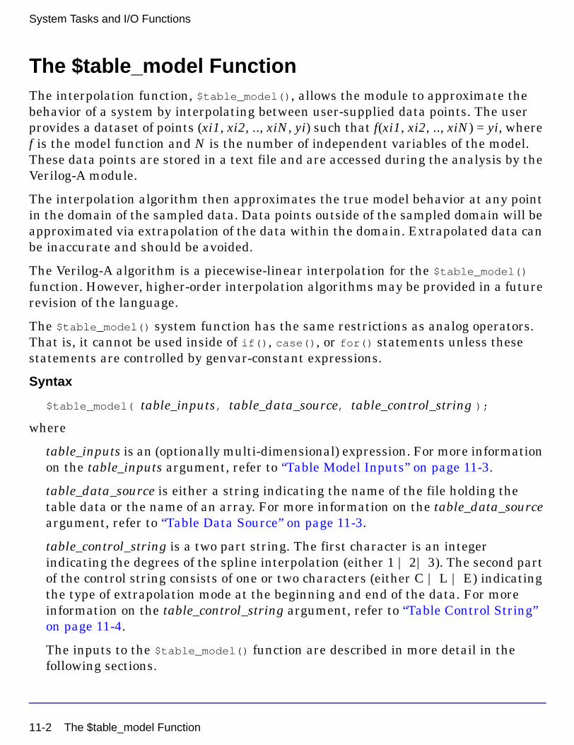
System Tasks and I/O Functions
The $table_model FunctionThe interpolation function, $table_model(), allows the module to approximate the behavior of a system by interpolating between user-supplied data points. The user provides a dataset of points (xi1, xi2, .., xiN, yi) such that f(xi1, xi2, .., xiN) = yi, where f is the model function and N is the number of independent variables of the model. These data points are stored in a text file and are accessed during the analysis by the Verilog-A module.
The interpolation algorithm then approximates the true model behavior at any point in the domain of the sampled data. Data points outside of the sampled domain will be approximated via extrapolation of the data within the domain. Extrapolated data can be inaccurate and should be avoided.
The Verilog-A algorithm is a piecewise-linear interpolation for the $table_model() function. However, higher-order interpolation algorithms may be provided in a future revision of the language.
The $table_model() system function has the same restrictions as analog operators. That is, it cannot be used inside of if(), case(), or for() statements unless these statements are controlled by genvar-constant expressions.
Syntax
$table_model( table_inputs, table_data_source, table_control_string );
where
table_inputs is an (optionally multi-dimensional) expression. For more information on the table_inputs argument, refer to “Table Model Inputs” on page 11-3.
table_data_source is either a string indicating the name of the file holding the table data or the name of an array. For more information on the table_data_source argument, refer to “Table Data Source” on page 11-3.
table_control_string is a two part string. The first character is an integer indicating the degrees of the spline interpolation (either 1 | 2| 3). The second part of the control string consists of one or two characters (either C | L | E) indicating the type of extrapolation mode at the beginning and end of the data. For more information on the table_control_string argument, refer to “Table Control String” on page 11-4.
The inputs to the $table_model() function are described in more detail in the following sections.
11-2 The $table_model Function

Table Model Inputs
The table_inputs are numerical expressions that are used as the independent model variables for the $table_model() function. They may be any valid expressions that can be assigned to an analog signal.
Table Data Source
The table_data_source argument specifies the source of sample points for the $table_model() function. The sample points may come from two sources: files and arrays. The file source indicates that the sample points be stored in a file, while the array source indicates that the data points are stored in a set of array variables. The user may choose the data source by either providing the file name of a file source or a set of array variables as an argument to the function.
The table is created when the $table_model() system function is called for the first time. Any changes to the table_data_source argument(s) of the $table_model() after the first call are quietly ignored (that is, the table model is not recreated). For a file source, each sample point of the table is represented as a sequence of numbers in the order of Xi1 Xi2 .. XiN Yi, where Xik is the coordinate of the sample point in kth dimension and Yi is the model value at this sample point. Each sample point must be separated by a new line. The numbers in the sequence must be separated by one or more spaces or tabs. Comments may be inserted before or after any sample point; comments must begin with ‘#’ and end with a new line.
The data file must be in text format only. The numbers must be real or integer. The sample points can be stored in the file in any order.
Example
The following example shows the contents of a table model files with two dimensions.
# datafile.tbl# 2-D table model sample example of the function# f(x,y) = sqrt(x^2 + y^2)## x y f(x,y)-2 -2 2.828-2 -1 2.236-1 -1 1.414 0 0 0 0 1 1.0 1 1 1.414
The $table_model Function 11-3

System Tasks and I/O Functions
1 2 2.236 2 2 2.828
If the source of the data is an array, a set of one-dimensional arrays that contain the data points must be passed to the $table_model() function. The size of these arrays is determined by the number of sample points in the table, M. The data are stored in the arrays such that for the kth dimension of the ith sample point, kth_dim_array_identifier[i] = Xik and such that for the ith sample point output_array_identifier[i] = Yi.
Example
For the previous table model example, the same data would be provided to the function in an array as shown in the following code fragment.
@(initial_step) beginx[0]=-2; y[0]=-2; f_table[0]=2.828; // 0th sample pointx[1]=-2; y[1]=-1; f_table[1]=2.236; // 1st sample pointx[2]=-1; y[2]=-1; f_table[2]=1.414; // 2nd sample pointx[3]=-0; y[3]= 0; f_table[3]=0;x[4]=-0; y[4]=-1; f_table[4]=1;x[5]=-0; y[5]=-1; f_table[5]=1.414;x[6]= 1; y[6]= 2; f_table[6]=2.236;x[7]= 2; y[7]= 2; f_table[7]=2.828;
end
Table Control String
The control string provides information on how the model should interpolate and extrapolate the table data. The control string consists of sub-strings for each dimension. Each sub-string may contain one character indicating the degree of the spine interpolation and an additional one or two characters indicating the type of extrapolation method to be used.
Table Interpolation Degree
The degree character is an integer between 1 and 3 representing the degrees of splines to be used for the interpolation. If not given, a degree of 1 (linear) is assumed. Table 11-1 shows the possible settings.
11-4 The $table_model Function

Extrapolation Control String
The extrapolation control string is used to control the algorithm to extrapolate beyond the supplied data domain. The string may contain one or two extrapolation method characters. The extrapolation method determines the behavior of the table model when the point to be evaluated is beyond the domain of the user provided sample points. The Clamp extrapolation method, specified with the character C, uses a constant value from the last data point to extend the model.The Linear extrapolation method, specified with the character L, uses piecewise linear interpolation to estimate the requested point. The user may also disable extrapolation by setting the Error extrapolation method using the character E. In this case, an extrapolation error is reported if the $table_model() function is requested to evaluate a point beyond the interpolation region. Table 11-2 summarizes these options.
For each dimension of the table, users may use up to two extrapolation method characters to specify the extrapolation method used for each end of the data set. When no extrapolation method character is supplied, the Linear extrapolation method will be used for both ends as default behavior. When a single extrapolation method character is supplied, the specified extrapolation method will be used for both ends of the data set. When two extrapolation method characters are supplied, the first character specifies the extrapolation method used for the end with the lower coordinate value and the second character specifies the extrapolation method for the
Table 11-1. Extrapolation Method Characters
Table Interpolation Character
Interpolation Character Description
1 Linear spline (degree 1)
2 Quadratic spline (degree 2)
3 Cubic spline (degree 3)
Table 11-2. Extrapolation Method Characters
Table Extrapolation Character
Extrapolation Character Description
C Clamp extrapolation
L Linear extrapolation (default)
E Error condition
The $table_model Function 11-5

System Tasks and I/O Functions
end with the higher coordinate value. Table 11-3 illustrates some control strings and their interpretation.
Examples
In the first example, the data from the table defined earlier is contributed across the ports. The data in both dimensions is linearly extrapolated at both ends of the data.
module table_resistor (n1, n2);electrical n1, n2;
analog beginI(n1, n2) <+ $table_model (V(n1), V(n2), "datafile.tbl", "1L,1L");
endendmodule
In the second example, the same information is supplied within the module using the array method.
module user_table(n1, n2);electrical n1, n2;real x[0:7], y[0:7], f_table[0:7];analog begin
@(initial_step) beginx[0]=-2; y[0]=-2; f_table[0]=2.828; // 0th sample pointx[1]=-2; y[1]=-1; f_table[1]=2.236; // 1st sample pointx[2]=-1; y[2]=-1; f_table[2]=1.414; // 2nd sample pointx[3]=-0; y[3]= 0; f_table[3]=0;x[4]=-0; y[4]=-1; f_table[4]=1;x[5]=-0; y[5]=-1; f_table[5]=1.414;x[6]= 1; y[6]= 2; f_table[6]=2.236;x[7]= 2; y[7]= 2; f_table[7]=2.828;
end
Table 11-3. Control String Examples
Control String Interpretation
"1LE,2EC" 1st dimension linear interpolation, linear extrapolation on left, error on extrapolation to right2nd dimension quadratic interpolation, error on extrapolation to left, clamp on extrapolation to right
"" Linear interpolation, Linear extrapolation to left and right
,2 1st dimension linear interpolation, 2nd dimension quadratic interpolation, linear extrapolation to left and right
"3,1" 1st dimension cubic interpolation, 2nd dimension linear interpolation, linear extrapolation to left and right
11-6 The $table_model Function

I(a, b) <+ $table_model (V(n1), V(n2), x, y, f_table, "1L,1L");endendmodule
File Input/Output OperationsThere are several functions to provide reading and writing to files on the operating system. $fopen() opens a file for output while $fclose() closes the file. $fstrobe(), $fdisplay, and $fwrite() provide functions to write to the file.
The $fopen Function
The file open function, $fopen(), returns a value whose bits indicate a corresponding channel available for writing. $fopen() opens the file specified as an argument and returns the next available 32-bit multichannel descriptor, which is unique for the file. If the file could not be found or opened for writing, it returns 0.
The multichannel descriptor can be considered to be a set of 32 flags, where each flag represents a single output channel. The least significant bit (bit 0) always represents standard output, also called channel 0, while the other bits represent channels which have been opened by $fopen().
The first call to $fopen() opens channel 1 and returns a value of 2 (bit 1 of the descriptor is set). The next call to $fopen() opens channel 2 and returns a value of 4 (bit 2 of the descriptor is set). Subsequent calls open channels 3, 4, 5, etc. and return values of 8, 16, 32, etc. A channel number corresponds to a single bit in the multichannel descriptor. Up to 32 channels may be opened.
Syntax
multi-channel_descriptor = $fopen( file_name );
where multi-channel_descriptor is an integer value and file_name is the name of the file to be opened.
The $fclose Function
The file close function, $fclose(), closes the specified channel in the multichannel descriptor. Further output to the closed channel is no longer allowed. The $fopen() function reuses channels which have been closed.
File Input/Output Operations 11-7

System Tasks and I/O Functions
Syntax
$fclose( multi_channel_descriptor );
where multi-channel_descriptor is an integer value representing the channel(s) to be closed.
The $fstrobe Function
The file strobe function, $fstrobe(), writes date to the channel(s) specified in the multichannel descriptor.
Syntax
$fstrobe(multi_channel_descriptor [, list_of_arguments ]);
where multi_channel_descriptor is represents one or more opened files and list_of_arguments is an optional, comma separated list of quoted strings or expressions. The arguments for list_of_arguments are the same as those available for the $strobe() function argument.
Example
integer multi_ch_desc1, multi_ch_desc2, data_value;@(initial_step) begin
multi_ch_desc1 = $fopen("data1.txt");multi_ch_desc2 = $fopen("data2.txt");data_value = 1;
end
$fstrobe(multi_ch_desc1 | multi_ch_desc2, "Write value %d to both data1.txt and data2.txt", data_value) ;
The $fdisplay Function
The file display function, $fdisplay(), writes date to the channel(s) specified in the multichannel descriptor. It provides the same capability as the $fstrobe() function.
Syntax
$fdisplay( multi_channel_descriptor [, list_of_arguments ]);
where multi_channel_descriptor is represents one or more opened files and list_of_arguments is an optional, comma separated list of quoted strings or expressions. The arguments for list_of_arguments are the same as those available for the $strobe argument.
11-8 File Input/Output Operations

The $fwrite Function
The file write function, $fwrite(), writes date to the channel(s) specified in the multichannel descriptor. It provides the same capability as the $fstrobe() function but without the newline character.
Syntax
$fwrite( multi_channel_descriptor [, list_of_arguments ]);
where multi_channel_descriptor is represents one or more opened files and list_of_arguments is an optional, comma separated list of quoted strings or expressions. The arguments for list_of_arguments are the same as those available for the $strobe() function argument.
Display Output OperationsThere are several functions available to display information to the user during a simulation. Each uses the same format specification but has slightly different modes of operation.
The $strobe Function
The strobe function, $strobe(), displays its argument when the simulator has converged for all nodes at that time point. The $strobe() function always appends a new line to its output. The $strobe() function returns a newline character if no arguments are passed.
Syntax
$strobe( list_of_arguments );
where list_of_arguments is a comma separated list of quoted strings or expressions.
Examples
$strobe("The value of X is %g", X);
$strobe(); // print newline
The $display Function
The display function, $display(), provides the same capability as the $strobe function but without the newline character.
Display Output Operations 11-9

System Tasks and I/O Functions
Syntax
$display( list_of_arguments );
Example
$display("\n\nWarning: parameter X is %g, max allowed is %g\n\n", X, maxX);
Format Specification
The following tables describe the escape sequences available for the formatted output. The hierarchical format specifier, %m, does not take an argument. It will cause the display task to output the hierarchical name of the module, task, function, or named block which invoked the system task using the hierarchical format specifier. This feature can be used to determine which module generated a message, in the case where many modules are instantiated.
Table 11-4. Escape Sequences
Sequence Description
\n newline character
\t tab character
\\ \ character
\" " character
\ddd character specified by 1-3 octal digits
%% % character
Table 11-5. Format Specifications
Specifier Description
%h or %H hexadecimal format
%d or %D decimal format
%o or %O octal format
%b or %B binary format
%c or %C ASCII format
%m or %M hierarchical name format
%s or %S string format
11-10 Display Output Operations

Simulator Control OperationsSimulator control functions provide a means to interrupt simulator execution.
The $finish Simulator Control Operation
The finish task simulator control operation, $finish, forces the simulator to exit and optionally print a diagnostic message.
Syntax
$finish [ (n) ];
where n is an optional flag to either (0) print nothing, (1) print simulator time and location, or (2) print simulator time, location, and statistics. The default value is 1.
Example
if (myError)$finish(1);
The $stop Simulator Control Operation
The stop simulator control option, $stop, suspends the simulator at the converged timepoint and optionally prints a diagnostic message.
Syntax
$stop [ (n) ];
where n is an optional flag to either (0) print nothing, (1) print simulator time and location, or (2) print simulator time, location, and statistics. The default value is 1.
Table 11-6. Format Specifications for Real Numbers
Specifier Description
%e or %E exponential format for real type
%f or %F decimal format for real type
%g or %G decimal or exponential format for real type using format that results in shorter printed output
Simulator Control Operations 11-11

System Tasks and I/O Functions
Example
if (myError)$stop(1);
11-12 Simulator Control Operations

Chapter 12: The Verilog-A/AMS PreprocessorVerilog-A provides a familiar set of language preprocessing directives for macro definitions, conditional compilation of code, and file inclusion. Directives are preceded by the accent grave ( ` ) character, which should not be confused with a single quote. The directives are:
`define
`else
`ifdef
`include
`resetall
`undef
Defining MacrosA macro is defined using the `define directive
`define name value
For example,
`define PI 3.14
defines a macro called PI which has the value 3.14. PI may now be used anywhere in the Verilog-A file after this definition. To use PI, the preprocessing directive character, accent grave ( ` ), must precede it. For example,
V(p,n) <+ sin(2*`PI*freq*time);
results in the following code
V(p,n) <+ sin(2*3.14*freq*time);
The directive name must be a valid identifier. It must be a sequence of alpha-numeric characters and underscores with a leading alpha character. Existing directive names cannot be used. This includes Verilog-A, Verilog-AMS and Verilog-2001 directives. Examples of invalid macro definitions are:
Defining Macros 12-1

The Verilog-A/AMS Preprocessor
`define undef 1 // existing Verilog-A directive - wrong!`define 1PICO 1p // leading character invalid - wrong!`define elsif 1 // Verilog 2001 directive - wrong!
Macro text may be presented on multiple lines by using the Verilog-A line continuation character, backslash (\), at the end of each line. The backslash must be the last character on the line. If white space is inserted after the continuation character then the system will not continue the line.
Macros may also be parameterized using an arbitrary number of arguments,
`define name(arg1,arg2,arg3…) value
For example,
`define SUM(A,B) A+B
defines a parameterized macro called SUM which may be subsequently used as
V(out) <+ `SUM(V(in1),V(in2))
Argument names must also be valid identifiers and are separated by commas. There can be no space between the name of the macro and the first parenthesis. If there is a space, then the parenthesis and all characters that follow it are taken to be part of the macro definition text.
Macros may be re-defined. Doing so will produce a compiler warning. They may also be undefined using the `undef directive:
`undef SUM
The `undef directive takes a single macro name as argument. Note that no directive character is used here. Using `undef on a macro that has not been defined results in a compiler warning.
All macros may be removed using the `resetall directive. This is not frequently used, as it effectively deletes all macros defined to this point in processing. The directive takes no arguments as
`resetall
Including FilesThe `include directive allows the inclusion of one file in another.
`include "filename"
12-2 Including Files

The `include directive accepts a single quoted string, a file name, as argument. If an absolute filename is given, the compiler looks for the referenced file. If a relative filename is given, the compiler first looks in the current working directory and then in the system include directory for the referenced file. In either case, if the file is found, its contents are inserted into the current file in place of the include directive. If the file is not found then the system issues an error message. The system include directory is given by
$HPEESOF_DIR/tiburon-da/veriloga/include
Most Verilog-A files begin by including disciplines.vams and constants.vams as
`include "disciplines.vams"`include "constants.vams"
The compiler finds these system include files in the system include directory above. Include directives may be nested to twenty levels deep.
Conditional CompilationCode may be conditionally compiled using the `ifdef-`else-`endif preprocessor construct. For example,
`ifdef macro statements`else statements`endif
If the conditional macro is defined, then the first set of statements are compiled, else the second set of statements are compiled. Both the true and false branches of the conditional must consist of lexicographically correct Verilog-A code. Note that as in undef, the preprocessing directive character is not used in the condition.
The else clause is optional and the construct may be written as,
`ifdef macro statements`endif
The following example performs output only if the DEBUG macro has been defined.
`ifdef DEBUG $strobe("Output Voltage:%e", V(out));`endif
Conditional Compilation 12-3
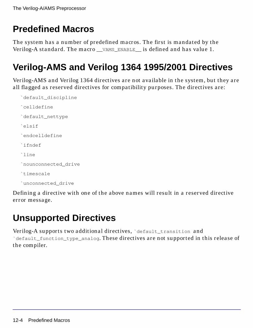
The Verilog-A/AMS Preprocessor
Predefined MacrosThe system has a number of predefined macros. The first is mandated by the Verilog-A standard. The macro __VAMS_ENABLE__ is defined and has value 1.
Verilog-AMS and Verilog 1364 1995/2001 DirectivesVerilog-AMS and Verilog 1364 directives are not available in the system, but they are all flagged as reserved directives for compatibility purposes. The directives are:
`default_discipline
`celldefine
`default_nettype
`elsif
`endcelldefine
`ifndef
`line
`nounconnected_drive
`timescale
`unconnected_drive
Defining a directive with one of the above names will result in a reserved directive error message.
Unsupported DirectivesVerilog-A supports two additional directives, `default_transition and `default_function_type_analog. These directives are not supported in this release of the compiler.
12-4 Predefined Macros

Appendix A: Reserved Words in Verilog-A/AMSThis appendix lists the reserved Verilog-A keywords. It also includes Verilog-AMS and Verilog-2001 keywords which are reserved.
A
abs and
absdelay asin
acos asinh
acosh assign
ac_stim atan
always atan2
analog atanh
analysis
B,C
begin casez
bound_step ceil
branch cmos
buf connectrules
bufif0 cos
bufif1 cosh
case cross
casex
D
ddt disable
deassign discipline
default discontinuity
defparam driver_update
delay
A-1

Verilog-A Keywords
E
edge endnature
else endprimitive
end endspecify
endcase endtable
endconnectrules endtask
enddiscipline event
endfunction exclude
endmodule exp
F,G,H
floor function
flow generate
for genvar
force ground
forever highz0
fork highz1
from hypot
I,J
idt initial_step
idtmod inout
if input
ifnone integer
inf join
initial
L,M,N
laplace_nd min
laplace_np module
A-2

laplace_zd nand
laplace_zp nature
large negedge
last_crossing net_resolution
limexp nmos
ln noise_table
log nor
macromodule not
max notif0
medium notif1
O,P
or pow
output primitive
parameter pull0
pmos pull1
posedge pullup
potential pulldown
R,S
rcmos sin
real sinh
realtime slew
reg small
release specify
repeat specparam
rnmos sqrt
rpmos strobe
rtran strong0
rtranif0 strong1
rtranif1 supply0
scalared supply1
A-3

Verilog-A Keywords
T
table tranif1
tan transition
tanh tri
task tri0
temperature tri1
time triand
timer trior
tran trireg
tranif0
V,W,X,Z
vectored wor
vt wreal
wait xnor
wand xor
weak0 zi_nd
weak1 zi_np
while zi_zd
white_noise zi_zp
wire
A-4

Appendix B: Unsupported ElementsTable B-1lists the unsupported Verilog-A keywords and functionality.
Table B-1. Unsupported Elements
Hierarchy: Ordered parameter lists in hierarchical instantiation
Hierarchical names, except for node.potential.abstol and node.flow.abstol, which are supported
Derived natures
The defparam statement
Functions: Accessing variables defined in a function’s parent module
Input / Output: The %b format character
The \ddd octal specification of a character
Parameter-sized ports
Enforcement of input, output, and inout
System tasks: $realtime scaled to the ‘timescale directive
The %b, %o, and %h specifications
$monitor
File operations
B-1

Unsupported Elements
B-2

Appendix C: Standard DefinitionsThis appendix lists the current values of the standard header files that are part of the distribution.
The disciplines.vams File/*Verilog-A definition of Natures and Disciplines$RCSfile: disciplines.vams,v $ $Revision: 1.1 $ $Date: 2003/09/22
01:36:17 $*/ `ifdef DISCIPLINES_VAMS`else`define DISCIPLINES_VAMS 1
discipline logicdomain discrete;enddiscipline/** Default absolute tolerances may be overriden by setting the* appropriate _ABSTOL prior to including this file*/// Electrical// Current in amperesnature Currentunits = “A”;access = I;idt_nature = Charge;
`ifdef CURRENT_ABSTOLabstol = `CURRENT_ABSTOL;`elseabstol = 1e-12;`endifendnature
// Charge in coulombsnature Chargeunits = “coul”;access = Q;ddt_nature = Current;`ifdef CHARGE_ABSTOLabstol = `CHARGE_ABSTOL;`elseabstol = 1e-14;
C-1

Standard Definitions
`endifendnature
// Potential in voltsnature Voltageunits = “V”;access = V;idt_nature = Flux;`ifdef VOLTAGE_ABSTOLabstol = `VOLTAGE_ABSTOL;`elseabstol = 1e-6;`endifendnature
// Flux in Webersnature Fluxunits = “Wb”;access = Phi;ddt_nature = Voltage;`ifdef FLUX_ABSTOLabstol = `FLUX_ABSTOL;`elseabstol = 1e-9;`endifendnature
// Conservative disciplinediscipline electricalpotential Voltage;flow Current;enddiscipline
// Signal flow disciplinesdiscipline voltagepotential Voltage;enddisciplinediscipline currentpotential Current;enddiscipline
// Magnetic
// Magnetomotive force in Ampere-Turns.nature Magneto_Motive_Forceunits = “A*turn”;access = MMF;`ifdef MAGNETO_MOTIVE_FORCE_ABSTOLabstol = `MAGNETO_MOTIVE_FORCE_ABSTOL;`elseabstol = 1e-12;
C-2

`endifendnature
// Conservative disciplinediscipline magneticpotential Magneto_Motive_Force;flow Flux;enddiscipline
// Thermal
// Temperature in Kelvinnature Temperatureunits = “K”;access = Temp;`ifdef TEMPERATURE_ABSTOLabstol = `TEMPERATURE_ABSTOL;`elseabstol = 1e-4;`endifendnature
// Power in Wattsnature Powerunits = “W”;access = Pwr;`ifdef POWER_ABSTOLabstol = `POWER_ABSTOL;`elseabstol = 1e-9;`endifendnature
// Conservative disciplinediscipline thermalpotential Temperature;flow Power;enddiscipline
// Kinematic// Position in metersnature Positionunits = “m”;access = Pos;ddt_nature = Velocity;`ifdef POSITION_ABSTOLabstol = `POSITION_ABSTOL;`elseabstol = 1e-6;`endifendnature
C-3

Standard Definitions
// Velocity in meters per secondnature Velocityunits = “m/s”;access = Vel;ddt_nature = Acceleration;idt_nature = Position;`ifdef VELOCITY_ABSTOLabstol = `VELOCITY_ABSTOL;`elseabstol = 1e-6;`endifendnature
// Acceleration in meters per second squarednature Accelerationunits = “m/s^2”;access = Acc;ddt_nature = Impulse;idt_nature = Velocity;`ifdef ACCELERATION_ABSTOLabstol = `ACCELERATION_ABSTOL;`elseabstol = 1e-6;`endifendnature
// Impulse in meters per second cubednature Impulseunits = “m/s^3”;access = Imp;idt_nature = Acceleration;`ifdef IMPULSE_ABSTOLabstol = `IMPULSE_ABSTOL;`elseabstol = 1e-6;`endifendnature
// Force in Newtonsnature Forceunits = “N”;access = F;`ifdef FORCE_ABSTOLabstol = `FORCE_ABSTOL;`elseabstol = 1e-6;`endifendnature
C-4

// Conservative disciplinesdiscipline kinematicpotential Position;flow Force;enddisciplinediscipline kinematic_vpotential Velocity;flow Force;enddiscipline
// Rotational
// Angle in radiansnature Angleunits = “rads”;access = Theta;ddt_nature = Angular_Velocity;`ifdef ANGLE_ABSTOLabstol = `ANGLE_ABSTOL;`elseabstol = 1e-6;`endifendnature
// Angular Velocity in radians per secondnature Angular_Velocityunits = “rads/s”;access = Omega;ddt_nature = Angular_Acceleration;idt_nature = Angle;`ifdef ANGULAR_VELOCITY_ABSTOLabstol = `ANGULAR_VELOCITY_ABSTOL;`elseabstol = 1e-6;`endifendnature
// Angular acceleration in radians per second squarednature Angular_Accelerationunits = “rads/s^2”;access = Alpha;idt_nature = Angular_Velocity;`ifdef ANGULAR_ACCELERATION_ABSTOLabstol = `ANGULAR_ACCELERATION_ABSTOL;`elseabstol = 1e-6;`endifendnature
// Torque in Newtonsnature Angular_Force
C-5

Standard Definitions
units = “N*m”;access = Tau;`ifdef ANGULAR_FORCE_ABSTOLabstol = `ANGULAR_FORCE_ABSTOL;`elseabstol = 1e-6;`endifendnature
// Conservative disciplinesdiscipline rotationalpotential Angle;flow Angular_Force;enddisciplinediscipline rotational_omegapotential Angular_Velocity;flow Angular_Force;enddiscipline
`endif
The constants.vams File/*Verilog-A definition of Mathematical and physical constants$RCSfile: constants.vams,v $ $Revision: 1.1 $ $Date: 2003/09/22 01:36:17
$*/`ifdef CONSTANTS_VAMS`else`define CONSTANTS_VAMS 1// M_ indicates a mathematical constant`define M_E 2.7182818284590452354`define M_LOG2E 1.4426950408889634074`define M_LOG10E 0.43429448190325182765`define M_LN2 0.69314718055994530942`define M_LN10 2.30258509299404568402`define M_PI 3.14159265358979323846`define M_TWO_PI 6.28318530717958647652`define M_PI_2 1.57079632679489661923`define M_PI_4 0.78539816339744830962`define M_1_PI 0.31830988618379067154`define M_2_PI 0.63661977236758134308`define M_2_SQRTPI 1.12837916709551257390`define M_SQRT2 1.41421356237309504880`define M_SQRT1_2 0.70710678118654752440
// P_ indicates a physical constant
C-6

// charge of electron in coulombs`define P_Q 1.6021918e-19
// speed of light in vacuum in meters/sec`define P_C 2.997924562e8
// Boltzman’s constant in joules/kelvin`define P_K 1.3806226e-23
// Plank’s constant in joules*sec`define P_H 6.6260755e-34
// permittivity of vacuum in farads/meter`define P_EPS0 8.85418792394420013968e-12
// permeability of vacuum in henrys/meter`define P_U0 (4.0e-7 * `M_PI)
// zero celsius in kelvin`define P_CELSIUS0 273.15
`endif
The compact.vams File/*Copyright 2002, 2003 Tiburon Design Automation, Inc. All rights reserved.This software has been provided pursuant to a License Agreementcontaining restrictions on its use. This software containsvaluable trade secrets and proprietary information of Tiburon Design Automation, Inc. and is protected by law. It may not be copied or distributed in any form or medium, disclosed to third parties, reverse engineered or used in any manner not provided for in said License Agreement except with the prior written authorization from Tiburon Design Automation, Inc.
Useful, common macro definitions and utilities$RCSfile: compact.vams,v $ $Revision: 1.1 $ $Date: 2003/09/22 01:36:17 $
*/
`ifdef COMPACT_VAMS`else`define COMPACT_VAMS 1// SPICE-specific different values:`define SPICE_GMIN 1.0e-12`define SPICE_K 1.3806226e-23 `define SPICE_Q 1.6021918e-19
`define LARGE_REAL 1.0e38`define MIN_CONDUCTANCE 1.0e-3`define DEFAULT_TNOM 27
C-7

Standard Definitions
/* NOT_GIVEN are codes that are used to detect if a* parameter value has been passed (future extensions * to Verilog-A should make this obsolete). */
`define NOT_GIVEN -9.9999e-99`define INT_NOT_GIVEN -9999999
`define N_MINLOG 1.0e-38`define MAX_EXP 5.834617425e14`define MIN_EXP 1.713908431e-15`define EXP_THRESHOLD 34.0
`define TRUE 1`define FALSE 0
/* Useful macro for setting Typeexample: `SET_TYPE(P_TYPE, N_TYPE, Type);will set variable Type */
`define SET_TYPE(n, p, Type) Type = 1; if (p == 1) Type = -1; if (n == 1) Type = 1
/* Print out value:example: `DEBUG_STROBE(“myVariable”, myVariable); */
`define DEBUG_STROBE(xName, x) \`ifdef DEBUG \
$strobe(“\n%s = %g”, xName, 1.0*x) \`else \
$strobe(““) \`endif
`endif
C-8

Appendix D: Condensed ReferenceVerilog-A is an analog hardware description language standard from Open Verilog International (www.ovi.org). It can be used to describe analog circuit behavior at a wide range of abstraction from behavioral models of circuits to compact transistor model descriptions. The Verilog-A source code is compiled automatically, if necessary, during a simulation. The netlist format follows the conventional ADS netlisting scheme. Modules whose names match ADS components will automatically override the built-in model description.
Verilog-A Module Template`include “disciplines.vams” // Natures and disciplines`include “constants.vams” // Common physical and math constantsmodule myModel(port1, port2);
electrical port1, port2;parameter real input1= 1.0 from [0:inf]; parameter integer input2 = 1 from [-1:1] exclude 0;real X;// this is a comment/* this is a * comment block */
analog begin @( initial_step ) begin
// performed at the first timestep of an analysisendif (input2 > 0) begin
$strobe(“input2 is positive”,input1)// module behavioral descriptionV(port1, port2) <+ I(port1, port2) * input1;
end@( final_step ) begin
// performed at the last time step of an analysisend
endendmodule
D-1

Verilog-A Condensed Reference
Data Types
Analog Operators and FiltersAnalog operators and filters maintain memory states of past behavior. They can not be used in an analog function.
Table D-1. Data Types
Data type Description
integer Discrete numerical type
integer [integer_name {, integer_name};
real Continuous numerical type
real[real_name {, real_name...};
parameter Attribute that indicates data type is determined at module instantiation.
parameter parameter_type param_name = default_value [from [range_begin:range_end] [exclude exclude_value];
Table D-2. Analog Operators and Filters
Operator Function
Time derivative The ddt operator computes the time derivative of its argument.
ddt(expr)
Time integral The idt operator computes the time-integral of its argument.
idt(expr, [ic [ , assert [ , abstol ] ] ] )
Linear time delay absdelay() implements the absolute transport delay for continuous waveform.
absdelay(input, time_delay [, maxdelay ])
D-2

Discrete waveform filters
The transition filter smooths out piecewise linear waveforms.
transition( expr [ , td [ , rise_time [ , fall_time [ , time_tol ] ] ] ] )
The slew analog operator bounds the rate of change (slope) of the waveform.
slew( expr [ , max_pos_slew_rate [ , max_neg_slew_rate ] ] )
The last_crossing() function returns a real value representing the simulation time when a signal expression last crossed zero.
last_crossing(expr, direction)
Laplace transform filters
laplace_zd() implements the zero-denominator form of the Laplace transform filter. The laplace_np() implements the numerator-pole form of the Laplace transform filter. laplace_nd() implements the numerator-denominator form of the Laplace transform filter. laplace_zp() implements the zero-pole form of the Laplace transform filter.
laplace_zp(expr, z, r)
Z-transform filters The Z-transform filters implement linear discrete-time filters. Each filter uses a parameter T which specifies the filter’s sampling period. The zeros argument may be represented as a null argument. The null argument is produced by two adjacent commas (,,) in the argument list.All Z-transform filters share three common arguments: T, t, and t0. T specifies the period of the filter, is mandatory, and must be positive. t specifies the transition time, is optional, and must be nonnegative.zi_zd() implements the zero-denominator form of the Z-transform filter. zi_np() implements the numerator-pole form of the Z-transform filter. zi_nd() implements the numerator-denominator form of the Z-transform filter. zi_zp() implements the zero-pole form of the Z-transform filter.
zi_zp( expr , z , r , T [ , t [ , t0 ] ] )
limexp Limits exponential argument change from one iteration to the next.
limexp(arg)
Table D-2. Analog Operators and Filters
Operator Function
D-3

Verilog-A Condensed Reference
Mathematical Functions
Table D-3. Mathematical Functions Supported by Verilog-A
Function Description Domain Return value
ln() natural log x>0 real
log(x) log base 10 x>0 real
exp(x) exponential X<80 real
sqrt(x) square root x>=0 real
min(x,y) minimum of x and y all x, y if either is real, returns real, otherwise returns the type of x,y.
max(x,y) maximum of x and y all x, y if either is real, returns real, otherwise returns the type of x,y.
abs(x) absolute value all x same as x
pow(x,y) xy if x>=0, all y;if x<0, int(y)
real
floor(x) floor all x real
ceil(x) ceiling all x real
D-4

Transcendental Functions
AC Analysis Stimuli
Table D-4. Transcendental Functions Supported by Verilog-A
Function Description Domain
sin(x) sine all x
cos(x) cosine all x
tan(x) tangent x != n (pi/2), n is odd
asin(x) arc-sine -1<= x <= 1
acos(x) arc-cosine -1<= x <= 1
atan(x) arc-tangent all x
atan2(x,y) arc-tangent of x/y all x, all y
hypot(x,y) sqrt(x2 + y2) all x, all y
sinh(x) hyperbolic sine x < 80
cosh(x) hyperbolic cosine x < 80
tanh(x) hyperbolic tangent all x
asinh(x) arc-hyperbolic sine all x
acosh(x) arc-hyperbolic cosine x >= 1
atanh(x) arch-hyperbolic tangent -1 <= x <= 1
Table D-5. AC Analysis Stimuli
Function Description
AC Stimulus The AC stimulus function produces a sinusoidal stimulus for use during a small-signal analysis.
ac_stim([analysis_name [, mag [, phase ]]])
D-5

Verilog-A Condensed Reference
Noise Functions
Analog Events
Table D-6. Noise Functions
Function Description
White Noise Generates a frequency-independent noise of power pwr.
white_noise(pwr [, name])
Flicker Noise Generates a frequency-dependent noise of power pwr at 1 Hz which varies
in proportion to the expression 1/fexp.
flicker_noise(pwr, exp [, name])
Noise Table Define noise via a piecewise linear function of frequency. Vector is frequency, pwr pairs in ascending frequencies.
noise_table(vector [, name])
Table D-7. Analog Events
Function Description
Initial Step Event trigger at initial step.
@(initial_step [(list_of_analyses)])
Final Step Event trigger at final step.
@(final_step [(list_of_analyses)])
Cross Zero crossing threshold detection.
cross(expr [ , dir [ , time_tol [ , expr_tol]]] );
Timer Generate analog event at specific time.
timer ( start_time [ , period [ , time_tol ] ] );
D-6

Timestep Control
Table D-8. Simulator Action Control Functions
Function Purpose
$bound_step Controls the maximum time step the simulator will take during a transient simulation.
$bound_step( expression );
$discontinuity Provides the simulator information about known discontinuities to provide help for simulator convergence algorithms.
$discontinuity [( constant_expression )];
D-7

Verilog-A Condensed Reference
Input/Output Functions
Simulator Environment FunctionsThe environment parameter functions return simulator environment information.
Table D-9. Input/Output Operations
Function Return Value
$strobe$display$write
Display simulation data when the simulator has converged on a solution for all nodes using a printf() style format.
$strobe(args)
$fopen Open a file for writing and assign it to an associated channel.
multi-channel_desc = $fopen("file");
$fclose Close a file from a previously opened channel(s).
$fclose(multi-channel_desc);
$fstrobe$fdisplay$fwrite
Write simulation data to an opened channel(s) when the simulator has converged. Follows format for $strobe.
$fstrobe(multi-channel_desc, "info to be written");
Table D-10. Environment Parameter Functions
Function Return Value
$temperature Return circuit ambient temperature in Kelvin.
$temperature
$abstime Return absolute time in seconds.
$abstime
D-8

Module HierarchyStructural statements are used inside the module block but cannot be used inside the analog block.
module_or_primative #({.param1(expr){, .param2(expr})} instance_name ({node {, node});
Example
my_src #(.fstart(100), .ramp(z));
$vt $vt can optionally have Temperature (in Kelvin) as an input argument and returns the thermal voltage (kT/q) at the given temperature. $vt without the optional input temperature argument returns the thermal voltage using $temperature.
$vt[(Temperature)]
$analysis Returns true (1) if current analysis matches any one of the passed arguments.
$analysis(str {, str} )
Table D-10. Environment Parameter Functions
Function Return Value
D-9

Verilog-A Condensed Reference
D-10

Index
Symbols$ (dollar sign), 3-4, 3-5$abstime function, 10-1$bound_step function, 10-2$discontinuity function, 10-3$display function, 11-9$dist_chi_square function, 6-11$dist_erlang function, 6-12$dist_exponential function, 6-10$dist_normal function, 6-9$dist_poisson function, 6-10$dist_t function, 6-11$dist_uniform function, 6-9$fclose function, 11-7$fdisplay function, 11-8$finish function, 11-11$fopen function, 11-7$fstrobe function, 11-8$fwrite function, 11-9$param_given function, 11-1$random function, 6-8, 10-5$rdist_chi_square function, 6-11$rdist_erlang function, 6-12$rdist_exponential function, 6-10$rdist_normal function, 6-9$rdist_poisson function, 6-10$rdist_t function, 6-11$rdist_uniform function, 6-9$realtime function, 10-1$stop function, 11-11$strobe function, 11-9$table_model function, 11-2$temperature function, 10-1$vt function, 10-2% (modulo), 6-8%m (hierarchical format specifier), 11-10) (right parenthesis), 4-5@ (at-sign operator), 8-1_ (underscore), 3-3, 3-4__VAMS_ENABLE__ (predefined macro),12-4` (accent grave), 3-5, 12-1`celldefine (reserved directive), 12-4`default_discipline (reserved directive),
12-4
`default_function_type_analog (unsupported directive), 12-4
`default_nettype (reserved directive), 12-4`default_transition (unsupported
directive), 12-4`define (compiler directive), 12-1`else (compiler directive), 12-1, 12-3`elsif (reserved directive), 12-4`endcelldefine (reserved directive), 12-4`endif (compiler directive), 12-3`ifdef (compiler directive), 12-1, 12-3`ifndef (reserved directive), 12-4`include (compiler directive), 12-1, 12-2`line (reserved directive), 12-4`nounconnected_drive (reserved
directive), 12-4`resetall (compiler directive), 12-1, 12-2`timescale (reserved directive), 12-4`unconnected_drive (reserved directive),
12-4`undef (compiler directive), 12-1, 12-2{ (left bracket), 4-4} (right bracket), 4-4, 4-5
Aabsolute delay operator, 7-3absolute tolerance, 7-2, 7-3, 7-5AC analyses, 7-4, 7-5ac_stim function, 10-5access functions, 2-3, 2-5
access function value, 2-2AHDL, 1-4ambient temperature, 10-1, 10-2analog behavior, 2-2, 5-1, 6-6, 8-1analog block, 2-2, 2-4, 5-1, 7-1
defining the analog block, 2-1, 2-2analog events, 8-3, 8-4analog expressions, 6-5analog functions, 2-4, 2-5, 2-8analog modeling, 1-1analog operators, 7-1, 7-6, 8-4, 8-5analog procedural block flow, 6-1analog signals, 1-2, 2-3, 4-2, 8-3analog statements, 5-4analysis dependent functions, 10-3
Index-1

arithmetic conversion, 6-6arithmetic operators, 6-2arrays, 4-1, 4-4, 7-1assignment order, 2-6attributes, 4-2automatic conversion of numeric types,
6-6
Bbackslash, 12-2backward compatibility, 3-5behavioral description, 2-1behavioral model, 8-1binary operators, 3-2bit-wise operators, 6-3block item declaration, 2-5block naming, 5-1block statements, 3-2bounds, 10-2branch contribution operator, 2-4branch contribution statement, 2-4branches, 2-3
Ccase sensitivity, 3-4case statements, 5-2, 7-1Chi-Square distribution, 6-11circular integrator operator, 7-3comma-separated lists, 4-4comments, 3-2compact models, 1-2, 1-6compiler directives, 3-5
`define, 12-1`else, 12-1, 12-3`endif, 12-3`ifdef, 12-1, 12-3`include, 12-1, 12-2`resetall, 12-1, 12-2`undef, 12-1, 12-2
compiler technology, 1-4complex constants, 3-3compound elements, 6-5concatenation operator, 6-5concurrency, 9-7conditional compilation, 12-1, 12-3conditional execution, 2-5conditional expressions, 7-1conditional macros, 12-3
conditional operators, 3-2, 6-4conditional statements, 5-1, 7-1connect modules, 9-8constant assignment value, 4-5constant expressions, 4-1, 4-4, 5-2constant numbers, 3-3, 4-4constants, 3-3continuous discipline, 4-3continuous domain, 2-3contribution operator, 2-3contribution statements, 2-3, 2-5, 8-5controlled transitions, 7-4convergence, 7-7
problems, 10-3properties, 7-1simulator, 11-9
cross function, 8-3
Ddata types, 4-1, 6-6DC analyses, 7-2, 7-4, 7-5, 7-6, 8-1decimal format, 3-3default parameter values, 2-6defining macros, 12-1delays on digital signals, 7-4derivative operator, 7-2digital signals, 1-2directives (see compiler & reserved
directives), 12-1, 12-4discipline resolution, 9-7disciplines, 4-2, 4-3
continuous disciplines, 4-3discipline data types, 4-1disciplines.vams file, 4-2, 12-3, C-1empty discipline, 4-2
discontinuities, 10-3discrete domain data types, 9-4discrete signals, 7-4, 7-6domain, 4-2, 4-3double quotes, 3-2
Eempty discipline, 4-2endpoint, 4-5environment parameter functions, 10-1Erlang random distribution, 6-12error messages, 12-3, 12-4escape sequences, 11-10
Index-2

event or operator, 8-5events, 8-1, 8-2
event expressions, 8-1event triggering, 8-5
exponentialfunctions, 7-1
expressions, 6-1, 8-5expression evaluation, 4-1, 6-5
Ffiles
constants.vams, 10-2, 12-3disciplines.vams, 4-2, 12-3, C-1file inclusion, 12-1
filters, 7-1Laplace transform, 7-8laplace_nd, 7-10laplace_np, 7-10laplace_zd, 7-9laplace_zp, 7-8slew, 7-4, 7-6transition, 7-4, 7-6, 10-3zi_nd, 7-14zi_np, 7-13zi_zd, 7-12zi_zp, 7-11Z-transform, 7-11
final_step, 8-2flicker_noise function, 10-5flow, 2-3, 4-2for statements, 5-4, 7-1format specifications, 11-10formfeeds, 3-2functions, 2-8, 3-5, 6-1, 6-6
$abstime, 10-1$bound_step, 10-2$discontinuity, 10-3$display, 11-9$dist_chi_square, 6-11$dist_erlang, 6-12$dist_exponential, 6-10$dist_normal, 6-9$dist_poisson, 6-10$dist_t, 6-11$dist_uniform, 6-9$fclose, 11-7$fdisplay, 11-8$finish, 11-11
$fopen, 11-7$fstrobe, 11-8$fwrite, 11-9$param_given, 11-1$random, 6-8, 10-5$rdist_chi_square, 6-11$rdist_erlang, 6-12$rdist_normal, 6-9$rdist_poisson, 6-10$rdist_t, 6-11$rdist_uniform, 6-9$realtime, 10-1$stop, 11-11$strobe, 11-9$table_model, 11-2$temperature, 10-1$vt, 10-2abs, 6-6ac_stim (AC stimulus), 10-5acos, 6-7acosh, 6-8analysis, 10-3asin, 6-7asinh, 6-7atan, 6-7atan2, 6-7atanh, 6-8ceil, 6-7cos, 6-7cosh, 6-7cross, 8-3exp, 6-6, 7-7flicker_noise, 10-5floor, 6-7hyperbolic, 6-6, 6-7hypot, 6-7last_crossing, 7-7limexp, 7-7, 10-3ln, 6-6log, 6-6mathematical, 6-6max, 6-6min, 6-6noise_table, 10-6pow, 6-7rdist_exponential, 6-10simulator, 10-1sin, 6-7
Index-3

sinh, 6-7sqrt, 6-6statistical, 6-8system, 6-8tan, 6-7tanh, 6-7thermal voltage (vt), 10-2timer, 8-4transcendental, 6-6, 6-7trigonometric, 6-7
GGaussian distribution, 6-9genvars, 4-4, 5-4, 7-1global events, 8-1global reference node, 2-4, 4-3global tolerance, 7-1ground, 2-4, 4-3
Hhardware description language, 1-1hierarchical descriptions
hierarchical format specifier, 11-10hierarchical models, 2-6
hyperbolic functions, 6-6, 6-7
Iidentifiers, 3-4ifdef-else-endif preprocessor construct,
12-3independent variables, 1-6index variable, 5-4indices, 4-1indirect branch assignment, 2-4initial condition, 7-2, 7-3initial_step global event, 8-1input parameters, 2-5instance
declaration, 2-6, 2-7parameters, 2-7
instantiatinga module, 2-6
integers, 3-3, 4-1, 6-6, 6-7, 8-3integration, 7-2intellectual property protection, 1-4interative approaches, 7-1
JJacobian, 1-5
Kkeywords, 3-1, 3-4, 3-5Kirchoff
voltage and current laws, 1-4
Llanguage
constructs, 3-4preprocessing directives, 12-1
languagesC, 1-2, 6-1HDL, 1-1mixed-signal, 1-2Verilog, 1-2Verilog-A, 1-2VHDL, 1-2
Laplace filters, 7-1, 7-8large-signal analysis, 10-5last_crossing function, 7-7lexical conventions, 3-1, 12-3limexp function, 10-3line continuation character, 3-1linear discrete-time filters, 7-11local
declaration of variables, 5-1tolerances, 7-1variables, 2-5
logical operators, 6-3looping statements, 7-1
Mmacros, 12-1, 12-2
macro definitions and utilities, 12-1, C-7predefined, 12-4
magnitude, 10-5mathematical
equations, 1-2, 1-6functions, 6-6
maximum slew rate, 7-6mixed-signal language, 1-2mixed-signal models, 9-1models, 1-2, 1-7, 6-1modules, 2-8
connect modules, 9-8module behavior, 10-3
Index-4

module boundary, 2-8module declaration, 2-1, 2-2, 2-6module instantiation
resistor example, 2-1module port definition, 2-7
modulus, 7-3monitored events, 8-1, 8-3multiple actions, 5-2
Nname spaces, 2-8named blocks, 2-5, 2-8natures, 4-2, C-1negative transitions, 7-5net_discipline, 4-2nets, 2-3, 2-4, 4-3
analog nets, 4-2implicit nets, 4-3neural nets, 1-2
newline character, 11-9newlines, 3-1, 3-2Newton-Raphson, 1-5, 7-1nodes, 1-4, 2-3, 2-4, 11-9noise, 4-1
noise contribution, 10-5, 10-6noise modeling, 10-5noise power, 10-6noise_table function, 10-6
nonlinear equations, 7-1normal distributions, 6-9null arguments, 8-1numbers, 3-1, 3-3
floating point, 3-3, 4-1integer, 3-3number type, 4-1real, 3-3scale factors, 3-3
OOP analyses, 7-4operands, 6-6, 6-7operating system, 11-7operators, 6-1
absdelay, 7-3arithmetic, 6-2binary (double), 3-2bit-wise, 6-3concatenation, 6-5
conditional, 6-4conditional (ternary), 3-2ddt, 7-2event or, 8-5idt, 7-2idtmod, 7-3limexp, 7-1logical, 6-3precedence, 6-5relational, 6-2shift, 6-4unary (single), 3-2
optimization, 1-1optional block identifier, 5-1ordered lists, 2-6, 2-7
Pparameters, 4-4
default parameter values, 2-6defining parameters, 2-1, 2-2, 2-4input parameters, 2-5instance parameters, 2-7parameter declaration, 2-6parameter description, 1-1parameter extraction, 1-3parameterized macros, 12-2seed_expression, 6-8
partial derivatives, 1-5passed variable arguments, 2-5phase, 10-5phase shift, 7-4piecewise
constant waveforms, 7-4continuous signal, 7-6linear, 7-5, 10-6
Poisson distribution, 6-10ports
defining ports, 2-1, 2-2mixed ports, 9-2port assignment, 2-7
positive transitions, 7-5potential, 2-3, 4-2power, 10-5
power spectral density, 10-6predefined macros, 12-4predefined mathematical constants
M_1_PI, C-6M_2_PI, C-6
Index-5

M_2_SQRTPI, C-6M_E, C-6M_LN10, C-6M_LN2, C-6M_LOG10E, C-6M_LOG2E, C-6M_PI, C-6M_PI_2, C-6M_PI_4, C-6M_SQRT1_2, C-6M_SQRT2, C-6M_TWO_PI, C-6
predefined non-escaped identifiers, 3-4predefined physical constants
P_C, C-7P_CELSIUS0, 10-2, C-7P_EPS0, C-7P_H, C-7P_K, C-7P_Q, C-7P_U0, C-7
preprocessing directives, 12-1procedural control statements, 5-1procedural statements, 2-2pseudo-random bit stream generator, 8-4pseudo-random numbers, 6-8
Rradians, 6-7, 10-5random number generation, 6-8range, 4-5real
constants, 3-3data types, 4-1declarations, 4-1numbers, 3-3
reference net, 2-4relational operators, 6-2relative filenames, 12-3repeat statements, 5-3, 7-1reserved directives, 12-4
`celldefine, 12-4`default_discipline, 12-4`default_nettype, 12-4`elsif, 12-4`endcelldefine, 12-4`ifndef, 12-4`line, 12-4
`nounconnected_drive, 12-4`timescale, 12-4`unconnected_drive, 12-4
Sscalar, 4-3
elements, 6-5scale factors, 3-3scientific notation, 3-3scope, 2-8seed_expression, 6-8sequential block, 5-1shift operators, 6-4short-circuiting, 6-5signal
access functions, 2-4data, 2-3
signal-flowbranch, 2-3net, 2-3
signed integers, 6-8simulation
simulation flow, 10-2simulator functions, 10-1
single line comment, 3-2slew filter, 7-4, 7-6slope, 7-6small-signal analyses, 7-4, 7-6, 10-5source branch relations, 2-4spaces, 3-1, 3-2SPICE, 1-4, 10-4standard deviation, 6-9statement block, 2-5statistical functions, 6-8strings, 3-1, 3-2, 10-3Student’s T distribution of values, 6-11synchronization, 9-7system include
directory, 12-3files, 12-3
system tasks and functions, 3-5system equations, 7-1system functions, 6-8
Ttabs, 3-1, 3-2tasks, 2-8temperature, 10-1
Index-6

thermal voltage, 10-2threshold crossings, 8-3time, 1-4
$abstime, 10-1$realtime, 10-1time delay, 7-4time derivative operator, 7-2time duration, 8-1time integral, 7-2time integrator operator, 7-2timer function, 8-4timesteps, 8-3, 10-2
tokens, 3-1, 3-2transcendental functions, 6-6, 6-7transient analysis, 10-5transition filter, 7-4, 7-6, 10-3trigonometric functions, 6-7type, 4-5type conversion, 4-1
Uunary operators, 3-2, 3-3underscore character, 3-3uniform distributions, 6-9unsupported directives
`default_function_type_analog, 12-4`default_transition, 12-4
user-definedfunctions, 2-4, 7-1tasks, 3-5types, 4-2
Vvariables, 1-6, 4-1varying waveforms, 7-4vectors, 2-3, 10-6Verilog, 1-2Verilog 1364, 12-4Verilog-2001, 12-1Verilog-A, 1-2
line continuation character, 12-2modules, 2-1
Verilog-AMS, 12-1, 12-4keywords, 3-4
VHDL, 1-2voltage contribution statement, 2-2
Wwarnings, 12-2waveforms, 7-5, 7-6while statements, 5-3, 7-1white noise, 10-5white space, 3-1, 3-2, 12-2
Zzero transmission, 7-6zero-crossing, 1-6Z-transform filters, 7-1, 7-11
Index-7

Index-8