Verification of Large Industrial Circuits

Using SAT Based Reparameterization

and Automated Abstraction-Refinement

Pankaj P. Chauhan

May 2007CMU-CS-07-123

School of Computer ScienceCarnegie Mellon University

Pittsburgh, PA 15213

Submitted in partial fulfillment of the requirementsfor the degree of Doctor of Philosophy.

Thesis Committee:Prof. Edmund M. Clarke, Chair

Prof. Randal E. BryantProf. James Hoe

Dr. Jin Yang, Intel

Copyright c© 2007 Pankaj P. Chauhan

This research was sponsored by the Semiconductor Research Corporation (SRC) under contractno. 99-TJ-684, the National Science Foundation (NSF) under grant no. CCR-9803774, the Officeof Naval Research (ONR), the Naval Research Laboratory (NRL) under contract no. N00014-01-1-0796, and the Army Research Office (ARO) under contract no. DAAD19-01-1-0485.

The views and conclusions contained in this document are those of the author and should not beinterpreted as representing the official policies, either expressed or implied, of SRC, NSF, ONR,NRL, ARO, or the U.S. government.

Keywords: Model Checking, Image Computation, Quantification Scheduling,SAT, Bounded Model Checking, Parametric Representation, Abstraction-Refinement

For my parents.

iv

Abstract

Automatic formal verification of large industrial circuits with thou-sands of latches is still a major challenge today due to the state spaceexplosion problem. Moreover, BDD based algorithms are very sensitiveto the variable ordering. Satisfiability (SAT) procedures have becomemuch more powerful over the last few years, and hence they have beenused in formal verification of large circuits with techniques like automatedabstraction refinement and ATPG.

This thesis addresses the capacity challenge at multiple levels. First,at the core, I provide new algorithms for both BDD based and SAT basedimage computation. Image computation involves efficient quantificationof variables from Boolean functions. I propose BDD based algorithmsthat use various combinatorial optimization techniques to obtain betterquantification schedules, and in the later part, consider novel non-linearquantification schedules. The SAT based image computation uses algo-rithms for efficiently enumerating satisfying assignments to a Booleanformula, and for storing the enumerated assignments. Building upon thisenumeration algorithm, I propose a novel SAT based reparameterizationalgorithm that increases the capacity of symbolic simulation by large ex-tent. The reparameterization algorithm recomputes a much smaller rep-resentation for the set of states, whenever the size of the representationof state set becomes too large in symbolic simulation. These improve-ments help in bounded model checking of large systems, by allowing formuch deeper depths. I demonstrate a 3x improvement in the runtime andspace requirement over existing BMC algorithm and BDD based symbolicsimulator on large industrial circuits. Finally, the reparameterization al-gorithm is incorporated in a SAT based automated abstraction-refinementframework. The reparamaterization algorithm can simulate much longerabstract counterexamples than previously possible. I then extract therefinement information from the simulation, completing the abstraction-refinement loop. Thus, contributions beginning at the core problem ofimage computation, through state space travesals and continuing all theway up to the abstraction-refinement are addressed in this thesis.

vi

Acknowledgments

The old adage that your thesis advisor is the only adult besides yourparents who mentors you for the longest period of time could not be truerin my case. Right from the beginning when Ed visited my undergraduateinstitution, he has been a constant source of inspiration and motivation.He would always have many problems you could work on, without worry-ing overly about the chance of success. The greatest virtue of Ed’s groupwas the continued interaction with the brilliant group of visitors, post-doctoral students and graduate students that he would assemble from allover the world. Above all, Ed has always believed in me through out mylong graduate studentship, and has been always there when I needed himin various ups and downs. I would like to express the deepest gratitudetowards my guru, for everything that he blessed me with.

Any mention of Ed is incomplete without Martha. She has alwaysbeen taking keen interested in the well being of Ed’s students, and I wasno exception, so I would like to say, thank you Martha. Thanks to theexcellent support staff that Ed had, especially Keith and Denny, whomade the life of Ed’s group much easier. My heartfelt thanks to SharonBurks, without whom CMU SCS is incomplete. She ties the whole schooltogether, and is a “mother figure” for graduate students, faculty and everyone else alike. Thanks also to Catherine Copetas and Deb Cavlovich.

Thanks to Somesh Jha and Helmut Veith for getting me started on realresearch at CMU. My work on BDD based image computation wouldn’thave been possible without Somesh’s suggestion and Helmut’s guidance.Yuan got myself and Dong Wang started on abstraction refinement, toresult in the first approach for automated abstraction refinement based onSAT. Helmut was again a mentor in that work. Thanks to Jim Kukula,Synopsys, we had a credible set of benchmarks for both image compu-tation and abstraction-refinement. The core of my thesis, SAT basedquantification procedure and the reparameterization algorithm, howeverwere born out of discussions with and the subsequent guidance of DanielKroning. Thanks are also due to Amit Goel, whose DATE paper was astarting point for SAT-based reparameterization. He was a joy to collab-orate with in the work we did on consistency of specifications, apart frombeing a good friend. Thanks also to Dong Wang, Samir Sapra, ShuvenduLahiri, Ofer Strichman, and many others for enlightining discussions.

I would also like to thank my thesis committee members, Randy, Jinand James, for providing helpful and timely feedback throughout. Randyhas always amazed me and I am sure most others with his sharp insight.Summer internships have always provided me with a varied and challeng-ing learning environment, so thanks to my mentors Bob Kurshan at thethen Bell Labs, Aarti Gupta and Pranav Ashar at NEC Labs, and JinYang at Intel. Special thanks to Sharad Malik, for his continued concern

and encouragement. Deep gratitude is also due to my funding sources,NSF, GSRC, SRC and CMU CSD, who made my studentship possible.

I have been fortunate enough to have great teachers, starting from mypoor inner city primary school, through high-school, my undergraduateinstitute IIT Kharagpur, all the way to CMU. Most sincere thanks to myteachers and the institutes, without whom I would simply not be here.

My current employer Calypto also deserves a very special thanks. An-mol, Gagan, Nikhil, Deepak and others have provided a very stimulating,productive and supportive environment, not to mention the continuedencouragement to finish up my thesis.

On a personal level, words can not describe my gratitude towards myparents. They always allowed me freedom to choose my own course inlife, despite having many differences of opinions. I can never forget whendad helped me sneak to the train station to get to the IIT admissionscounseling, where my fruitful higher education began. I also want tothank my brother Ashish and sister Priti for their love and support.

Thanks so much to Maithili, the woman behind this man, for alwaysbeing there, taking care of Atharva, our son, and other things, and formaking many sacrifices to put my research before everything.

I can never forget my friends and co-conspirators Chirag Parikh, Prag-nesh Tewar, Malay Haldar, Sagar Chaki and others for putting up withme through and through.

Lastly, I am sure I am forgetting many who made a difference in mylife, so apologies and sincere thanks to them.

viii

Contents

1 Introduction 1

1.1 Formal Verification Challenges . . . . . . . . . . . . . . . . . . . . . . 3

1.2 Image Computation and Reachability Analysis . . . . . . . . . . . . . 6

1.3 Bounded Model Checking . . . . . . . . . . . . . . . . . . . . . . . . 9

1.4 Parametric Representation . . . . . . . . . . . . . . . . . . . . . . . . 11

1.5 Abstraction Refinement . . . . . . . . . . . . . . . . . . . . . . . . . 14

1.6 Scope of the Thesis . . . . . . . . . . . . . . . . . . . . . . . . . . . . 15

1.6.1 Image Computation . . . . . . . . . . . . . . . . . . . . . . . . 16

1.6.2 SAT Based Reparameterization . . . . . . . . . . . . . . . . . 17

1.6.3 Reparameterization for Abstraction-Refinement . . . . . . . . 19

1.7 Outline of the Dissertation . . . . . . . . . . . . . . . . . . . . . . . . 19

2 Image Computation and Reachability Analysis 21

2.1 Heuristic Methods and Dependency Matrices . . . . . . . . . . . . . . 27

2.1.1 Minimizing λ is NP-complete . . . . . . . . . . . . . . . . . . 32

2.1.2 Ordering Clusters by Hill Climbing . . . . . . . . . . . . . . . 33

2.1.3 Ordering Clusters by Simulated Annealing . . . . . . . . . . . 34

2.1.4 Ordering Clusters Using Graph Separators . . . . . . . . . . . 35

2.2 Non-linear Quantification Scheduling . . . . . . . . . . . . . . . . . . 38

2.3 Results for BDD Based Image Computation . . . . . . . . . . . . . . 44

2.4 SAT Procedures . . . . . . . . . . . . . . . . . . . . . . . . . . . . . . 51

2.5 SAT Procedures for Reachability Analysis . . . . . . . . . . . . . . . 53

2.5.1 Efficient Implementation of SAT Based Reachability . . . . . . 56

2.5.2 Cube Enlargement . . . . . . . . . . . . . . . . . . . . . . . . 58

2.5.3 Efficient Set Representation . . . . . . . . . . . . . . . . . . . 61

ix

2.5.4 Complexity of the Set Representation . . . . . . . . . . . . . . 63

2.6 Results for SAT Based Reachability Analysis . . . . . . . . . . . . . . 66

2.7 Related Work . . . . . . . . . . . . . . . . . . . . . . . . . . . . . . . 68

2.8 Summary . . . . . . . . . . . . . . . . . . . . . . . . . . . . . . . . . 71

3 SAT Based Reparameterization Algorithm for Symbolic Simulation 73

3.1 Introduction . . . . . . . . . . . . . . . . . . . . . . . . . . . . . . . . 73

3.2 Parametric Representation . . . . . . . . . . . . . . . . . . . . . . . . 75

3.3 Reparameterization using SAT . . . . . . . . . . . . . . . . . . . . . . 80

3.3.1 Background . . . . . . . . . . . . . . . . . . . . . . . . . . . . 80

3.3.2 Computing h1i and hc

i . . . . . . . . . . . . . . . . . . . . . . . 82

3.3.3 Computing h0i and h1

i in a single SAT run . . . . . . . . . . . 86

3.3.4 Incremental SAT . . . . . . . . . . . . . . . . . . . . . . . . . 87

3.3.5 Extensions to Handle General Transition Relations . . . . . . 88

3.4 Checking Safety Properties . . . . . . . . . . . . . . . . . . . . . . . . 91

3.4.1 Safety Property Checking . . . . . . . . . . . . . . . . . . . . 91

3.4.2 Counterexample Generation . . . . . . . . . . . . . . . . . . . 92

3.5 Experimental Results . . . . . . . . . . . . . . . . . . . . . . . . . . . 93

3.6 Fixed-Points with Reparameterization . . . . . . . . . . . . . . . . . 95

3.6.1 Set Union with an Auxiliary Variable . . . . . . . . . . . . . . 96

3.6.2 Fixed-Points by Using Stall Signal . . . . . . . . . . . . . . . . 97

3.7 Summary . . . . . . . . . . . . . . . . . . . . . . . . . . . . . . . . . 99

4 SAT Based Reparameterization in an Abstraction-Refinement Frame-work 101

4.1 Introduction . . . . . . . . . . . . . . . . . . . . . . . . . . . . . . . . 101

4.2 SAT Based Abstraction-Refinement . . . . . . . . . . . . . . . . . . . 104

4.2.1 Abstraction in Model Checking . . . . . . . . . . . . . . . . . 104

4.2.2 Generation of Abstract State Machine . . . . . . . . . . . . . 108

4.2.3 Bounded Model Checking in Abstraction-Refinement . . . . . 113

4.2.4 Refinement Based on Scoring Invisible Variables . . . . . . . . 116

4.2.5 Refinement Based on Conflict Dependency Graph . . . . . . . 117

4.3 Reparameterization in Abstraction-Refinement . . . . . . . . . . . . . 122

x

4.4 Experimental Results for Refinement . . . . . . . . . . . . . . . . . . 123

4.5 Summary . . . . . . . . . . . . . . . . . . . . . . . . . . . . . . . . . 129

5 Conclusions and Future Directions 131

A Proof of Theorem 1 135

B Proof of Theorem 3 139

C Proof of Theorem 4 149

xi

xii

List of Figures

1.1 A counter state machine. . . . . . . . . . . . . . . . . . . . . . . . . . 7

1.2 A circle in the xy plane. . . . . . . . . . . . . . . . . . . . . . . . . . 12

2.1 Reachability algorithm . . . . . . . . . . . . . . . . . . . . . . . . . . 22

2.2 Hill climbing algorithm for minimizing λ . . . . . . . . . . . . . . . . 33

2.3 Simulated annealing algorithm to minimize λ . . . . . . . . . . . . . . 35

2.4 An ordering algorithm based on graph separators . . . . . . . . . . . 37

2.5 Kernighan-Lin partition . . . . . . . . . . . . . . . . . . . . . . . . . 37

2.6 Basic step of the VarScore algorithms . . . . . . . . . . . . . . . . . . 40

2.7 Dynamic VarScore algorithm in action. The dotted lines represent theBDDs in the set F at different iterations of the VarScoreBasicStep. 42

2.8 Basic DPLL backtracking search (used from [61] for illustration purposes) 52

2.9 Outline of the SAT based reachability algorithm . . . . . . . . . . . . 55

2.10 Procedure ComputeSignature. . . . . . . . . . . . . . . . . . . . . . 62

2.11 Procedures AddCube. . . . . . . . . . . . . . . . . . . . . . . . . . . . 64

3.1 High Level Description of the Reparameterization Algorithm . . . . . 83

4.1 A counter state machine to illustrate abstraction and refinement. . . . 107

4.2 The counter state machine of Figure 4.1 encoded with 3 bits. . . . . . 109

4.3 Approximation to the abstract state machine of Figure 4.2(B) obtainedby pre-quantifying invisible variable v3. . . . . . . . . . . . . . . . . . 112

4.4 A spurious counterexample showing failure state [25]. No concretepath can be extended beyond failure state. . . . . . . . . . . . . . . . 114

4.5 Two dependent conflict graphs. Conflict B depends on conflict A,as the conflict clause ω9 derived from the conflict graph A producesconflict B. . . . . . . . . . . . . . . . . . . . . . . . . . . . . . . . . . 118

xiii

4.6 The unpruned dependency graph and the dependency graph (withindotted lines) . . . . . . . . . . . . . . . . . . . . . . . . . . . . . . . . 119

4.7 Scatter plots of simulation time and total time. A point above they = x line (diagonal) is a win for the new algorithm, and a pointbelow the line is a win for the FMCAD02 algorithm. . . . . . . . . . 127

A.1 (a) An instance of Optimal Linear Arrangement, (b) its reduction toλ−OPT . The permutation v1, v2, v3, v5, v4 is a solution to both. . . . 136

xiv

List of Tables

2.1 Correlation between various lifetime metrics and runtime/space for arepresentative sample of benchmarks. . . . . . . . . . . . . . . . . . . 45

2.2 Comparing FMCAD00, Kernighan-Lin separator (KLin) and Simu-lated annealing (SA) algorithms. (MOut)–Out of memory, (†)–SFEISTEL,(*)–8 reachability steps, (**)–14 reachability steps, (#)–13 reachabilitysteps. The lifetimes reported are after the final ordering phase. . . . . 47

2.3 Comparing lifetimes for various methods . . . . . . . . . . . . . . . . 49

2.4 Comparing our three static algorithms VS-I, VS-II and VS-III againstFMCAD00 and Simulated annealing (SA) algorithm. (MOut)–Out ofmemory, (†)–SFEISTEL, (*)–after 8 reachability steps, (**)–after 14reachability steps. . . . . . . . . . . . . . . . . . . . . . . . . . . . . . 50

2.5 Experimental results on a set of circuits from various sources includingISCAS’89 and Synopsys. The comparison is against [57]. Note: (*)-reachability was not complete. Empty boxes denote results N/A. . . . 67

3.1 Notations and Conventions. . . . . . . . . . . . . . . . . . . . . . . . 78

3.2 Experimental Results on Large Industrial Benchmarks comparing plainBMC against SAT-based reparameterization. . . . . . . . . . . . . . . 94

4.1 Circuits used for abstraction-refinement experiment. . . . . . . . . . . 125

4.2 Comparison of SAT based reparameterization against plain SAT basedsimulation in abstraction-refinement framework. . . . . . . . . . . . . 126

xv

xvi

Chapter 1

Introduction

Formal verification of hardware and software systems has come a long way over the

years to become an integral part of the product life cycle. There are numerous exam-

ples of well publicized hardware and software errors, such as the historically famous

FDIV bug in the Pentium processors (1994), the software glitch that led to the de-

struction of the NASA Orion-3 rocket (1998), the shutdown of the north-eastern US

power grid (2003), or the shutdown of the BART commuter rail system in San Fran-

cisco Bay area (2005). It is then no surprise that formal analysis has found its most

prominent use in finding errors in the systems. Apart from finding errors, formal

analysis is used for proving the correctness of the system under consideration, for di-

agnosis of errors, for design, for planning and discovery, or to prove that the system

meets certain specifications, such as timing requirements of various components on

a chip. Hardware verification has already become an industry unto itself, with es-

tablished EDA vendors, startups and internal R&D groups of chip makers providing

tools for property verification, equivalence checking, directed simulation, and so on.

The attractiveness of formal verification for hardware designers comes from the com-

pleteness of the formal verification with respect to state space exploration. Unlike

1

simulation and testing, formal verification analyzes each and every possible behavior

of the system to provide an all inclusive proof of correctness. In the software verifica-

tion, tools range from light weight static analysis tools such as Java Pathfinder and

Coverity, to full blown model checkers such as SPIN, SLAM, and to classical Hoare

style deductive proof engines such as NuPrl.

Formal methods [8, 29, 71] fall broadly under two categories, deductive methods,

such as theorem proving [9, 41] and inductive methods such as model checking [24].

In theorem proving, a system and the specifications to be verified are modeled as

axioms in a mathematical theory, and following a set of well founded inference rules,

a deductive proof of the correctness is obtained, either automatically or by some hu-

man guidance. Theorem proving has traditionally been very effective in proving that

a system satisfies certain specifications, and in dealing with infinite state systems.

Hoare style proofs are used to prove the correctness of many fundamental algorithms,

such as quick-sort. However, theorem proving usually requires a lot of human ex-

pertise. Moreover, if there is actually a bug in the system, demonstrating an error

trace from the failure of the proof is often difficult. Model checking on the other

hand is a technique where the state space of the system under considers is explored

systematically in its entirety to reason about the property being verified. The system

being verified is modeled as an automata, and the property to be verified is specified

using certain mathematical logics, such as linear temporal logic (LTL) or computation

tree logic (CTL). Model checking is an automated method, that requires little or no

user guidance. Moreover, model checking methods actually provide a counterexample

trace if the property being verified does not hold for the system. This is a very useful

diagnosis tool for system designers. Unlike theorem proving, an incomplete specifica-

tion is easily accepted by model checking, allowing for an incremental development of

both the model and the properties hand in hand with verification. However, model

2

checking techniques usually do not work well with infinite state systems. There have

been many successful applications of model checkers, both industrial and academic.

1.1 Formal Verification Challenges

In spite of all the advances in formal verification, many challenges still need to be

actively addressed. Active research, both from academia and industry alike, is being

pursued on the following axes. As the primary focus of this thesis is on model

checking, we will bias the discussion toward model checking.

Capacity

With ever increasing complexity of the systems, the size of the problems that need to

be solved by formal verification tools grows exponentially. The increase in complexity

results in the state explosion problem for model checking. Formal verification tools

run on for days without producing any results, or run out of memory for many

modern designs. The capacity limitations of model checkers and equivalence checkers

often restrict their use to block level or even sub-block level verification. Moreover,

it is often difficult to predict in advance whether a problem is tractable for formal

verification tool or not. For example, a model checker may be able to prove some

localized properties on a very large design, but may not be able to make progress on

a much smaller design that has some hard operators, such as multipliers. The lack of

predictability and capacity limitations of model checkers make it difficult to replace

traditional simulation and testing from the design flow. Instead, formal verification

is used to complement existing simulation and testing.

3

Usability

Another complaint against formal verification is the difficulty of use. Specifically,

building a specification for the system, which will form the basis of verification often

proves to be a daunting task for even the experienced users. The designers of the

system are usually most knowledgeable about the system and its intended behavior,

but they tend to be averse to using formal logics for specifying properties. The

verification engineer on the other hand has the expertise of formal verification, but

does not have the detailed system knowledge or specification. Efforts are being made

to make easier to specify properties using derivatives of temporal logics such as IBM

Sugar, PSL, or assertions in the hardware domain. In the software domain, executable

specification languages such as Z and state charts are gaining popularity. Lightweight

tools for software verification usually focus on certain classes of properties, such as

null pointer dereference, or violation of locking discipline. These comprise more than

90% of errors found in software.

Lack of Completeness

Theorem proving and model checking both rely on a set of properties being speci-

fied, and the correctness of the system is checked with respect to those properties.

However, the set of properties specified may not capture the full intent of the system

specification. Formal verification tools only verify the system against given proper-

ties. For example, a verification engineer may specify all the properties related to the

arithmetic and logical unit of a processor, but may not have enough specifications

about the instruction fetch unit. The process of completely and faithfully translating

an English language specification into a set of properties is a nontrivial task, often

requiring substantial human expertise. Coverage metrics are used in the testing and

4

simulation domain, such as the number of lines covered by the simulation. However,

given an LTL property, the coverage achieved by the property is difficult to define.

One can think of a fraction of reachable states that satisfy a given property as a

reasonable metric, but it does not relate well directly to the source code.

Lack of Diagnosis

Even though model checking provides a counterexample trace if a property fails, it is

often difficult to pin-point the cause of the error. It would be very helpful to indicate

a location or a set of locations in the source code that cause the error. Analysis of a

counterexample to find the source of the error, and to fix the error, is usually a manual

effort intensive process, requiring many iterations. Moreover, many a times, the error

is usually caused by under-constrained environment. In that case, the environment

constraints need to be refined.

Active research is being pursued to address all the challenges mentioned. In order

to address the capacity issues, the following directions are being pursued. First, the

fundamental data structures and algorithms used for state space exploration, such

as BDDs [10] and SAT [63] engines, are continuously being improved. In compo-

sitional reasoning [42, 51], a large verification problem is broken down into smaller

subproblems, and the proofs of correctness of the subproblems are assembled together

to derive the correctness of the whole system. Abstraction has always been used to

focus only on the relevant portion of the design for verifying a property. Abstraction

has been a manual process, but significant advances [23] have been made to make the

process of abstraction, and refinement of abstractions completely automatic. Next,

bounded model checking [5] is used to verify that the system satisfy a given property

for a bounded number of steps. If the bound is sufficiently large, than bounded model

checking suffices to conclude that the property is always true. If one uses equivalence

5

checking for proving the functional correctness, one does not need to specify prop-

erties. However, a golden model needs to be established to compare a given design

against. Establishing a golden model is a one time process, however, and one can

devote enough resources to specify the correctness of the golden model in a complete

manner. One a golden model is achieved, subsequent implementations can be checked

for equivalence against the golden model, leveraging the effort spent in establishing

the golden model in subsequent runs. In order to ease the diagnosis, sophisticated

error trace analyzers [37] are used to pinpoint the cause of the error.

Next, we describe few important aspects of a successful verification tool, and

briefly highlight the shortcomings in existing approaches.

1.2 Image Computation and Reachability Analy-

sis

Consider the state transition system depicted in Figure 1.1. The transition system

is a simple counter that counts from 0 to 3, upon receiving the input count. Let

the counter begin in the state 0. After one transition, the counter could be either

at state 1, or state 0, depending upon whether the input count was received or not.

The image of a set of states under a transition relation is the set of states reachable

from the given set of states in one transition. Thus, {0, 1} is the image of the set of

states {0}. Similarly, {0, 1, 2} is the image of the set of states {0, 1}. Pre-image is

the reverse of image. In the example, the pre-image of the set of states {0, 1, 2} is

{2, 1}. Intuitively, it denotes the set of states that can reach the given set of states

in one transition. Formally, given a transition system M = (S,R, S0), where S is the

set of states, R(s, s′) is the transition relation, and S0 is the initial set of states, the

6

image of a set of states Si is

Img(Si) = {s′|∃s ∈ Si.R(s, s′)}. (1.1)

Analogously, the pre-image operation is defined as

PreImg(Si) = {s|∃s′ ∈ Si.R(s, s′)}. (1.2)

0

3 2

1

count

count

count

count

!count!count

!count!count

Initial State

Figure 1.1: A counter state machine.

Image computation forms the core of all the state space traversal engines, includ-

ing model checking and inductive invariant proofs. The foremost application that

comes to mind is that of reachability, i.e., computing the set of states reachable from

the set of initial states Si. In out counter example, we can see that after one more

image computation, we get the set of states {0, 1, 2, 3}, which is all the states in the

state machine. Thus, we reach a fixed point, in fact, a least fixed point. In general,

we keep on computing the union of the set of states after every image computation,

and this process terminates when we reach a fixed point. Obviously, if the state space

is infinite, a fixed point may never be reached. Formally, we can define the reachable

7

set of states as the fixed point of the following function.

f(x) = x ∪ Img(x).

To denote a least fixed point of a function f(x), the notation µx.f(x) from µ-calculus

is often used. So, the set of reachable states is the fixed point

µx.(x ∪ Img(x)).

In model checking, there exists a fixed point characterization of all temporal logic

operators. For example, the set of states satisfying the CTL property EF p is given

by the following least fixed point at Sp, which is the set of states satisfying the atomic

predicate p.

µx.(x ∪PreImg(x)).

Since image computation is at the heart of model checking algorithms, it needs to

be as efficient as possible. The algorithm used for image computation obviously de-

pends on the underlying representation of the set of states and the transition relation,

used by a model checker. However, one needs to provide an efficient quantification

procedure for (pre) image computation, as per Equation 1.1 or Equation 1.2, no

matter what representation is used. For BDD based image computation, one needs

to quantify present (next) state variables and input variables for image (pre-image)

computation. Moreover, instead of building a single monolithic BDD for the tran-

sition relation, implicitly conjoined BDDs for transition relations of individual state

variables are commonly used. This is mostly done for capacity reasons, as building

a single monolithic BDD for transition relation is often infeasible in practice. This

representation is known as conjunctively partitioned transition relation. Synchronous

systems, e.g., hardware designs, readily yield such conjunctively partitioned transition

relations. For image computation, one needs to conjoin all the individual transition

8

relations and conjoin it with the BDD for the present state set. In order to avoid

blow up in BDD sizes during image computation, state variables are quantified as

soon as possible, in early quantification. We propose many new procedures for early

quantification, that are superior to existing, static approaches for early quantification.

It is well known that while BDDs are compact representations of many functions,

they unfortunately suffer from size explosion for many circuits. A BDD based model

checker is like a black box. A slight change in circuit or variable order can make model

checking infeasible. Moreover, there are some functions like multipliers, where the

BDDs are always exponentially large in the number of variables. BDD based model

checkers do not have a gradual degradation in performance, and the performance

is often not predictable. Modern SAT solvers have become very powerful over the

years, and thus provide an alternative to BDDs. Thus, we also offer a SAT based

image computation and reachability procedure that is robust and degrades gradually.

The runtime of our algorithm depends only on the size of the input circuit and on

the longest shortest path between an initial state and any reachable state, commonly

referred to as the diameter of the circuit. The existential quantification needed for

image computation is carried out by enumerating satisfying assignments to SAT

formulas and storing them in an efficient manner. The enumeration procedure for

computing existential quantification is central to the SAT based image computation

algorithm. This procedure also forms the core of reparameterization algorithms we

propose later.

1.3 Bounded Model Checking

In regular model checking, image or pre-image computation is carried out until a

fixed point, corresponding to the property being verified, is reached. Bounded model

9

checking on the other hand searches for counterexamples to a given LTL property

within a certain bound k. For the simple counter shown earlier in Figure 1.1, let us

consider the LTL property AG(counter < 3). This property is obviously false, and

the path 0, 1, 2, 3 is a counterexample to it. However, note that the shortest length

of a counterexample is 4. If we were bounded model checking the LTL property with

a bound of 3, we would not find a counterexample to the property. Bounded model

checking was proposed by Biere et al. [5] to overcome the limitations of BDDs, just at

the time when SAT procedures were becoming more powerful. In their formulation

of bounded model checking for safety property AG p, a propositional formula is

built that corresponds to the given transition relation R(s, s′) being unwound for k

transitions (the depth of the bounded model checking), starting from initial states

I(s0), and the failure of the property is checked after the k time steps, i.e., the

following propositional formula is built,

I(s0) ∧R(s0, s1) ∧R(s1, s2) ∧ . . . ∧R(sk−1, sk) ∧ ¬p(sk)

The formula above is satisfiable if and only if there exists a counterexample to

the property of length k. A satisfying assignment to the above formula provides a

trace in the state variables at times 0, 1, ..., k that violates the property. If there

doesn’t exist a counterexample to the property within k transition, the bound k is

increased, and the same process is repeated, until either the SAT procedure runs out

of resources, or sufficient depth is reached. The sufficient depth for a given transition

relation and the given property is called completeness threshold [27,28], which could

be quite large in practice. The basic technique above can be extended to do inductive

proofs as well. The inductive methods, such as proposed by Sheeran et al. [67], prove

that if the property holds for k transitions starting from any state, then the property

holds for k + 1 transitions as well. Coupling this with the proof of the property for

the first k transitions, i.e., the transitions from the initial states, we get a complete

10

proof of the property.

Since the original paper on bounded model checking, apart from the sophistica-

tion in the bounded model checking itself, SAT solvers have come a long way. This

has increased the scope of bounded model checking many fold. SAT based tech-

niques outperform BDD based techniques for many classes of verification problems.

Therefore, SAT based bounded model checking has become the preferred method for

bug finding. A comprehensive survey of bounded model checking and SAT based

verification techniques can be found in [6,63]. A detailed comparison of various SAT

based bounded and unbounded model checking techniques in an industrial setting is

provided in [2].

Despite all the advances, certain limitations are still encountered in practice for

bounded model checking. The main problem is that the difficulty of SAT problems

keeps on increasing as the bound k for bounded model checking is increased. This

limits the depth of the bounded model checking runs to a few tens of transitions

at most in practice. The usefulness of BMC as a complete verification technique is

jeopardized in the light of the fact that the completeness thresholds for most realistic

designs are large. Sometimes, computing the completeness thresholds of the design is

as hard as BMC itself. The technique of reparameterization that forms a large part

of this thesis attempts to alleviate the problem of deeper BMC depths by re-encoding

a set of states exactly as soon as the unrolled circuit becomes large.

1.4 Parametric Representation

Consider a circle of radius R in a 2-dimensional plane, centered at co-ordinates (0, 0),

shown in Figure 1.4. All the points (x, y) on the circle are described by the following

11

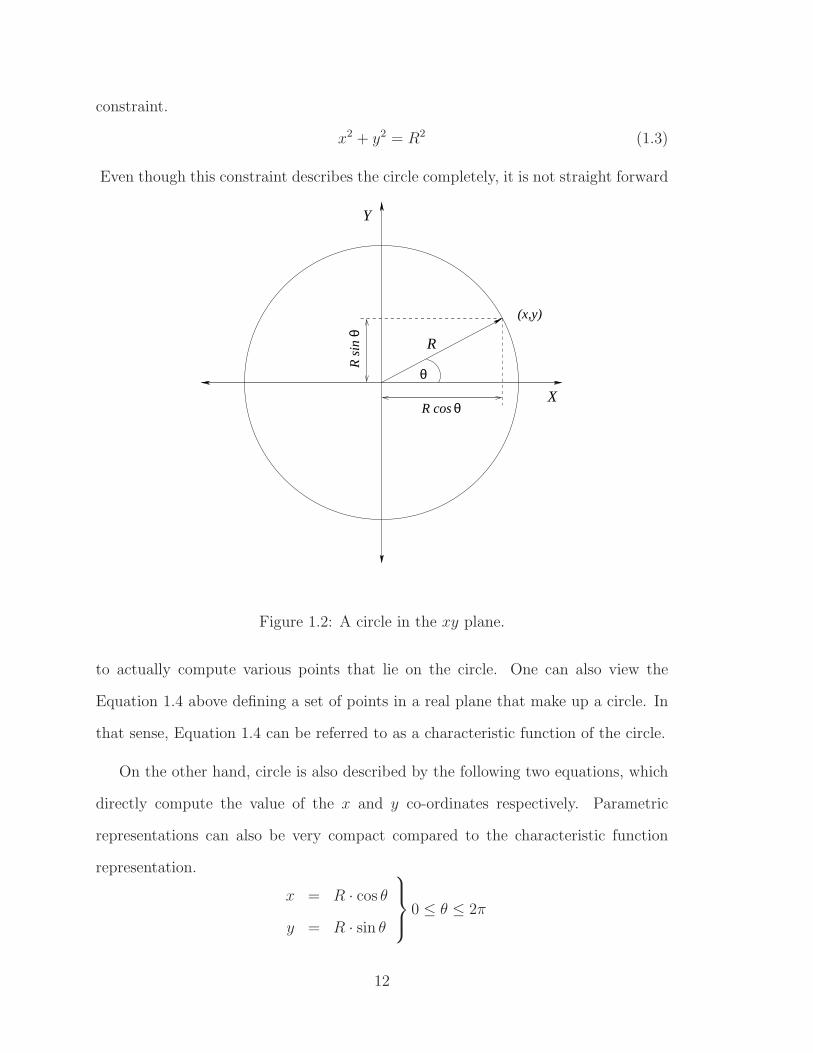
constraint.

x2 + y2 = R2 (1.3)

Even though this constraint describes the circle completely, it is not straight forward

R s

in θ

R cos θX

Y

(x,y)

R

θ

Figure 1.2: A circle in the xy plane.

to actually compute various points that lie on the circle. One can also view the

Equation 1.4 above defining a set of points in a real plane that make up a circle. In

that sense, Equation 1.4 can be referred to as a characteristic function of the circle.

On the other hand, circle is also described by the following two equations, which

directly compute the value of the x and y co-ordinates respectively. Parametric

representations can also be very compact compared to the characteristic function

representation.

x = R · cos θ

y = R · sin θ

0 ≤ θ ≤ 2π

12

The two representations can also be carried over to the Boolean domain. Consider

the set of states {01, 10}, with x1 and x2 as the state variables. We can represent

this set of states using the characteristic function

(x1 ∧ ¬x2) ∨ (¬x1 ∧ x2).

The same set of states can be given by the parametric representation

x1 = p, x = ¬p.

Here, p is a Boolean parameter. Note that parametric representation is not unique.

For the same set of states, we can also use

x1 = q1 ∧ q2, x2 = ¬q1 ∨ ¬q2,

which is not as compact as the first parametric representation. It can be easily shown

that one can always have a parametric representation with n or fewer parameters for

a set of vectors of n Boolean variables.

Parametric representations arise naturally in symbolic simulation, where a set of

expressions describing the values of state variables is built by unrolling the circuit,

as is done in BMC. After unrolling a circuit for k transitions, we have an expression

for each state variable. Primary inputs for each transition, and state variables of

each transition are the variables present in each expression. These variables can be

seen as the parameters that make up the parametric representation for the set of

states after k transitions. This parametric representation however is not compact,

and it grows linearly with the number of transitions. The same set of states could

be described compactly using n parameters or less, where n is the number of state

variables. Coming up with compact, efficient parametric representations is a major

part of this thesis. We propose novel SAT based method for reparameterizations. We

show that using SAT based reparameterization, one can perform much deeper depth

13

BMC. The existing approaches to parametric representation are based on BDDs, and

they suffer the usual drawbacks of BDD based methods. Specifically, as the number

of transitions in an unrolling increases, the number of BDD variables increases. BDDs

are much less robust to number of variables compared to SAT based methods, which

is the primary advantage of our method.

1.5 Abstraction Refinement

Symbolic model checking has been successful at automatically verifying temporal

specifications on small to medium sized designs. However, the inability of BDD

based model checking to handle large state spaces of “real world” designs hinders

the wide scale acceptance of these techniques. There have been advances on various

fronts to push the limits of automatic verification. On the one hand, improving BDD

based algorithms improves the ability to handle large state machines, while on the

other hand, various abstraction algorithms reduce the size of the design by focusing

only on relevant portions of the design. It is important to make improvements on

both fronts for successful verification.

A conservative abstraction is one which preserves all the behaviors of a concrete

system. Conservative abstractions benefit from a preservation theorem which states

that the correctness of any universal (e.g. ACTL∗) formula on an abstract system

automatically implies the correctness of the formula on the concrete system. On the

other hand, a counterexample on an abstract system may not correspond to any real

path, in which case it is called a spurious counterexample. To get rid of a spurious

counterexample, the abstraction needs to be made more precise via refinement. It is

obviously desirable to automate this procedure.

In Counterexample guided abstraction refinement (CEGAR) [3, 23, 25, 36, 49, 62],

14

an abstract counterexample is checked for validity on the original transition system.

If it is found to be invalid, then the abstraction is refined. SAT-based Unbounded

model checking [53,54] combines the ideas of bounded model checking, and abstrac-

tion refinement. It uses BMC on the abstract system to infer that no counterexamples

exist of a certain depth, and then unsatisfiability proofs of BMC to derive the refine-

ment. This thesis presents one of the earlier methods for SAT based CEGAR. Most

abstraction-refinement methods, including our method, rely on an effective procedure

for symbolic simulation of the original circuit, which could be very large. The SAT

reparameterization algorithm we present is used to make deeper symbolic simulation

efficient.

1.6 Scope of the Thesis

This thesis addresses the capacity challenge on multiple fronts. First, at the core,

I provide new algorithms for both BDD based and SAT based image computation.

The SAT based image computation uses an algorithm for enumerating satisfying

assignments to a Boolean formula, and an efficient representation of the enumerated

assignments. Building upon this enumeration algorithm, I propose a novel SAT

based reparameterization algorithm that increases the capacity of symbolic simulation

by a large extent. These improvements help in bounded model checking of large

systems. Finally, the reparameterization algorithm is incorporated in a SAT based

abstraction-refinement framework, thus providing completeness for safety and liveness

properties. Thus, improvements beginning at the core problem of image computation

and continuing it way up to the abstraction-refinement are addressed in this thesis.

15

1.6.1 Image Computation

We begin with new algorithms for BDD based image computation. I evaluate several

new heuristics, metrics, and algorithms for the problem of quantification schedul-

ing, central to BDD based image computation. The algorithms use combinatorial

optimization techniques such as hill climbing, simulated annealing, and ordering by

recursive partitioning to obtain better results than was previously the case. Theoret-

ical analysis and systematic experimentation are used to evaluate the algorithms. In

the second part of the project, I provide non-linear quantification scheduling. Until

then, quantification scheduling in image computation, with a conjunctively parti-

tioned transition relation, had been restricted to a linear schedule. This results in

a loss of flexibility during image computation. We view image computation as a

problem of constructing an optimal parse tree for the image set. The optimality of a

parse tree is defined by the largest BDD that is encountered during the computation

of the tree. We present dynamic and static versions of a new algorithm, VarScore,

which exploits the flexibility offered by the parse tree approach to the image compu-

tation. We show by extensive experimentation that our techniques outperform the

best known techniques so far.

Satisfiability procedures have shown significant promise for symbolic simulation

of large circuits, hence they have been used in many formal verification techniques,

including automated abstraction refinement, ATPG etc. I describe how to use mod-

ern SAT solvers like Chaff and GRASP to compute images of sets of states and

how to efficiently detect fixed point of the sets of states during reachability analy-

sis. Our method is completely SAT based, and does not use BDDs at all. The sets

of states and transition relation are represented in clausal form, which can be pro-

cessed by SAT checkers. The SAT checker subsequently generates the set of newly

reached states in a clausal form as well. At the heart of our engine lie two efficient

16

algorithms. The first algorithm shortens the cubes that the SAT checker generates,

which significantly reduces the number of cubes the SAT checker needs to enumerate.

The second algorithm reduces the space required to store sets of states as a set of

cubes by a recursive cube-merging procedure. The effectiveness of the SAT based

image computation procedure is demonstrated on ISCAS sequential benchmarks for

reachability. In particular, the algorithm does not have BDD size explosion surprises

and deteriorates in a predictable manner. There are many improvements to be done

to the enumeration procedure. A major improvement will be the use of non-clausal

representation for state sets. The interpolation proof based approach [54] provides

one possibility to explore.

1.6.2 SAT Based Reparameterization

I describe a SAT-based algorithm to perform the reparameterization step for symbolic

simulation. The algorithm performs better than BDD-based reparameterization espe-

cially in the presence of many input variables. The algorithm takes arbitrary Boolean

equations as input. Therefore, it does not require BDDs for the symbolic simulation.

Instead, non-canonical forms that grow linearly with the number of simulation steps

can be used. In essence, the SAT-based reparameterization algorithm computes a

new parametric function for each state variable one at a time. In each computa-

tion, a large number of input variables are quantified by a single call to a SAT-based

enumeration procedure [18, 53]. The advantage of this approach is two-fold: First,

all input variables are quantified at the same time, and second, the performance of

SAT-based enumeration procedure is largely unaffected by the number of input vari-

ables that are quantified. I demonstrate the efficiency of this new technique using

large industrial circuits with thousands of latches. I compared it to both SAT-based

Bounded Model Checking and BDD-based symbolic simulation. This new algorithm

17

can go much deeper than a standard Bounded Model Checker can. Moreover, the

overall memory consumption and the run times are, on average, 3 times less than

the values measured using a Bounded Model Checker. The BDD-based symbolic

simulator could not even verify most of the circuits that we used. There are various

research problems to be solved for using this algorithm for complete verification of

safety and liveness properties.

Safety property checking requires generation of a SAT formula from reparameter-

ized form. For the symbolic simulator, the counterexample generation is nontrivial,

since we do not keep the whole simulation. Periodically, we reparameterize the rep-

resentation and hence lose the information about input variables up to that point. I

next provide algorithms for safety property checking and counterexample generation

for the symbolic simulator. Invariant statements are often used to restrict the state

space for verification. Such invariants are often called verification conditions [43].

The technique described so far assumes that the transition relation is given by a set

of transition functions. It does not allow any arbitrary transition relation. I propose

extensions to handle both invariant constraints and general transition relations.

The algorithm can also benefit from the improvements to the basic SAT-based

enumeration algorithm. One limitation of the SAT-based enumeration algorithm is

the clausal (CNF or DNF) representation it uses. There are certain class of Boolean

functions which have no compact clausal representation. There has been some exist-

ing work in SAT based enumeration algorithms [44,53,68]. At present, the symbolic

simulator handles only safety properties. Biere et al. [66] recently showed that check-

ing for liveness properties can be done by a semantic translation to safety properties

with auxiliary variables. I briefly explore the computation of fixed-points using my

symbolic simulator.

18

1.6.3 Reparameterization for Abstraction-Refinement

Abstraction-refinement algorithms that simulate concrete systems benefit immensely

from a powerful simulator. I use my symbolic simulation algorithm for simulating

abstract counterexamples on concrete systems as in [19] or for doing BMC on concrete

systems as in [55]. The refinement information in both approaches is obtained from

the analysis of failed SAT instances (these correspond to spurious counterexamples,

meaning the abstraction needs to refined). One issue with using reparameterization

algorithm for refinement is that the SAT problem does not contain the information of

the simulation from the initial state. The SAT problem only contains the trace from

the last time frame when reparameterization was done to the length of the failed

counterexample state. I investigate the effect of doing refinement based on such

truncated counterexamples. Integrating my symbolic simulation with abstraction-

refinement will allow complete model checking of safety properties. Along with the

semantic translation of liveness properties to safety properties as in [66], handling

liveness properties should also be possible.

1.7 Outline of the Dissertation

The first half of Chapter 2 proposes new algorithms for BDD based image compu-

tation that rely on novel quantification scheduling technique. In the second half of

Chapter 2, we move on to SAT based image computation. The core of the SAT

based forward image computation is a SAT based algorithm for existential quantifi-

cation. The existential quantification algorithm is used as a building block for SAT

based reparameterization for symbolic simulation, described in Chapter 3. The SAT

based reparameterization algorithm allows us to simulate symbolically a circuit by

periodically re-encoding the set of reachable states. Chapter 4 describes an impor-

19

tant application of the reparameterization algorithm, namely the simulation used to

validate abstract counterexample on concrete machine in an automated abstraction-

refinement framework. Finally, we conclude in Chapter 5, with directions for future

research.

20

Chapter 2

Image Computation and

Reachability Analysis

Computing the set of states reachable in one step from a given set of states under

a transition relation forms the heart of many symbolic state exploration algorithms,

including reachability analysis, model checking [21, 22, 24], etc. This operation is

called image computation. Let us consider a state transition relation T over the set

of states S. The set of states is defined by the set of valuations over a vector of state

variables x. We denote a set or a vector of variables in a boldface. The transition

relation T (x, i,x′) relates states defined by valuations of present state variables x

and inputs i to states defined by valuations of next state variables x′. Note that we

are using characteristic functions S(x) and T (x, i,x′) to represent sets of states and

sets of transitions respectively. The image of S(x) under T (x, i,x′) is given by the

following equation.

Img(S(x′)) = ∃x, i.T (x, i,x′) ∧ S(x) (2.1)

21

Image computation is a major bottleneck in verification. In this chapter, we

will present various methods for efficient computation of images, both with BDDs

and with SAT solvers. For BDD based image computation, often it is infeasible to

construct BDDs for the transition relation T and the set S. In SAT based image

computation, we use propositional formulas in CNF with intermediate variables to

represent these sets, often resulting in much a smaller representation. The definition

of image computation involves evaluation of simple quantified Boolean formulas [18].

In reachability analysis, beginning with the set of initial states S0, images are

repeatedly computed until the set of states does not grow any more, in other words,

the least fixed-point, beginning at S0, given below is computed.

µX.(X ∪ Img(X)) (2.2)

Following simple algorithm computes this fixed-point.

Reachability(S0)

1 Sreach ← φ

2 S0 ← φ

3 i← 0

4 while (Si 6= φ) {

5 Sreach ← Sreach ∪ Si

6 Si+1 ← Img(Si)\Sreach

7 i← i + 1

8 }

9 return Sreach

s0 s1 s2 sk

sreach

. . .

Figure 2.1: Reachability algorithm

In this algorithm, Si denotes the set of newly discovered states in each iteration.

22

Once there are no more states to be discovered, we have reached a fixed-point.

As noted earlier, the sets of states and sets of transitions are traditionally repre-

sented by BDDs ( [10,13,14,24]). Canonicity of BDDs and compactness of represen-

tation for many functions encountered in practice allows for very efficient fixed point

checks. It is well known that while BDDs are compact representations of many func-

tions, they unfortunately suffer from size explosion for many circuits. A BDD based

model checker is like a black box. A slight change in circuit or variable order can make

model checking infeasible. For example, arithmetic functions like adders need to have

the inputs interleaved for linear sized BDD, while non-interleaved order leads to an

exponential blowup in BDD size. BDD based model checkers do not have a gradual

degradation in performance, and the performance is often not predictable. Thus, we

also offer a SAT based image computation and reachability procedure that is robust

and degrades gradually. The runtime of our algorithm depends only on the size of

the input circuit and on the longest shortest path between an initial state and any

reachable state, commonly referred to as the diameter of the circuit. An enumeration

procedure for computing existential quantification is central to the SAT based image

computation algorithm. This procedure also forms the core of reparameterization

algorithms described in the next chapter.

23

BDD Based Image Computation

In this section, we describe BDD based image computation algorithms. First, we

need to set up some preliminaries.

Notation: Every state is represented as a vector b1 . . . bn ∈ {0, 1}n of Boolean val-

ues. The transition relation R is represented by a Boolean function T (x1, . . . , xn,

x′1, . . . , x

′n). Note that we will drop the explicit mention of input variables. Vari-

ables X = x1, x2, . . . , xn and X ′ = x′1, x

′2, . . . , x

′n are called current state and next

state variables respectively. T (X,X ′) is an abbreviation for T (x1, . . . , xn, x′1, . . . , x

′n).

Similarly, functions of the form S(X) = S(x1, . . . , xn) describe sets of states. We will

occasionally refer to S as the set, and to T as the transition relation. For simplicity

we will use X to denote both the set {x1, . . . , xn} and the vector 〈x1, . . . , xn〉. Then

the set of variables on which f depends is denoted by Supp(f).

Example 1 [3 bit counter. (Running Example)] Consider a 3-bit counter with

bits x1, x2 and x3. x1 is the least significant and x3 the most significant bit. The state

variables are X = x1, x2, x3, X ′ = x′1, x

′2, x

′3. The transition relation of the counter

can be expressed as

T (X,X ′) = (x′1 ↔ ¬x1) ∧ (x′

2 ↔ x1 ⊕ x2) ∧ (x′3 ↔ (x1 ∧ x2)⊕ x3).

In later examples, we will compute the image Img(S) of the set S(X) = ¬x1. Note

that S(X) contains those states where the counter is even.

Partitioned BDDs: For most realistic designs it is impossible to build a single

BDD for the entire transition relation. Therefore, it is common to represent the tran-

sition relation as a conjunction of smaller BDDs T1(X,X ′), T2(X,X ′), . . . , Tl(X,X ′),

24

i.e.,

T (X,X ′) =∧

1≤i≤l

Ti(X,X ′),

where each Ti is represented as a BDD. The sequence T1, . . . , Tl is called a partitioned

transition relation. Note that T is not actually computed, but only the Ti’s are kept

in memory.

Example 2 [3 bit counter, ctd.] For the 3 bit counter, a very simple partitioned

transition relation is given by the functions T1 = (x′1 ↔ ¬x1), T2 = (x′

2 ↔ x1 ⊕ x2)

and T3 = (x′3 ↔ (x1 ∧ x2)⊕ x3).

Partitioned transition relations appear naturally in hardware circuits where each

latch (i.e., state variable) has a separate transition function. However, a partitioned

transition relation of this form typically leads to a very large number of conjuncts.

A large partitioned transition relation is similar to a CNF representation. So as the

number of conjuncts increases; the advantages of BDDs are gradually lost. Therefore,

starting with a very fine partition T1, . . . , Tl obtained from the bit relations, the

conjuncts Ti are grouped together into clusters C1, . . . , Cr, r < l such that each Ci is

a BDD representing the conjunction of several Ti’s. The image Img(S) of S is given

by the following expression.

Img(S(X)) = ∃X · (T (X,X ′) ∧ S(X)) (2.3)

= ∃X · (∧

1≤i≤l

Ti(X,X ′) ∧ S(X)) (2.4)

= ∃X · (∧

1≤i≤r

Ci(X,X ′) ∧ S(X)) (2.5)

Note that in general, an existential quantifier does not distribute over conunction.

Consequently, to compute Img(S(X)), formula 2.5 instructs us to compute first a

BDD for∧

1≤i≤r Ci(X,X ′)∧S(X). As argued above, partitioned transition relations

have been introduced to avoid computing this potentially large BDD.

25

Early Quantification: Under certain circumstances, existential quantification can

be distributed over conjunction using early quantification [13,70]. Early quantification

is based on the following observation: if we know that α does not contain x, then

∃x(α & β) is equivalent to α & (∃xβ). In general, we have l conjuncts and n

variables to be quantified. Since loosely speaking, clusters correspond to semantic

entities of the design to be verified, it is expected that not all variables appear in all

clusters. Therefore, some of the quantifications may be shifted over several Ci’s. For

a given sequence C1, . . . , Cr of clusters, we obtain

Img(S(X)) = ∃X1 · (C1(X,X ′) ∧ ∃X2 · (C2(X,X ′) . . .

∃Xr · (Cr(X,X ′) ∧ S(X)))) (2.6)

where Xi is the set of variables which do not appear in Supp(C1) ∪ . . . ∪ Supp(Ci−1)

and each Xi is disjoint from each other. Existentially quantifying out a variable

from a formula f reduces |Supp(f)|, which usually results in a reduced BDD size.

The success of early quantification strongly depends on the order of the conjuncts

C1, . . . , Cr. If we look at the parse tree of this equation, we see that it is a linear chain

of conjunctions and quantifications. Generalizing this for an arbitrary parse tree, a

variable can be quantified away at a subtree node as soon as it does not appear in

the rest of the tree.

Quantification Scheduling. The size of the intermediate BDDs in image compu-

tation can be reduced by addressing the following two questions:

Clustering: How to derive the clusters C1, . . . , Cr from the bit-relations T1, . . . , Tl

?

Ordering: How to order the clusters so as to minimize the size of the intermediate

BDDs?

26

These two questions are not independent. In particular, a bad clustering results

in a bad ordering. Moon and Somenzi [60] refer to this combined problem as the

quantification scheduling problem. The ordering of clusters is known as the conjunc-

tion schedule. Traditionally, only linear conjunction schedules have been considered.

Later on, we generalize this concept to arbitrary parse trees of the image computation

equation.

2.1 Heuristic Methods and Dependency Matrices

In this section, we propose algorithms for BDD based image computation that follow

traditional linear quantification schedules. The main contributions of this work are

the following:

• We extend and analyze image computation techniques previously developed by

Moon et al. [59]. These techniques are based on the dependence matrix of the par-

titioned transition relation. We explore various lifetime metrics related to this rep-

resentation and argue their importance in predicting costs of image computation.

Moreover, we provide effective heuristic techniques to optimize these metrics.

•We show that the problem of minimizing the lifetime metric of [59] is NP-complete.

More importantly, the reduction used to prove this NP-completeness result explains

the close connection between efficient image computation and the well studied prob-

lem of computing the optimal linear arrangement for an undirected graph.

•We model the interaction between various sub-relations in the partitioned transition

relation as a weighted graph and introduce a new class of heuristics called ordering

by recursive partitioning.

• We have performed extensive experiments which indicate the effectiveness of our

techniques.

27

The main conclusion to be drawn from our analysis is the following: For com-

plicated industrial designs, the effort initially spent on ordering algorithms is clearly

amortized during image computation. In other words, the benefits of good orderings

outweigh the cost of slow combinatorial optimization algorithms.

Our algorithms are based on the concepts of dependence matrices (introduced

in [59,60]) and sharing graphs.

Definition 1 (Moon et al) The dependence matrix of an ordered set of func-

tions {f1, f2, . . . , fm} depending on variables x1, . . . , xn is a matrix D with m rows

and n columns such that dij = 1 if function fi depends on variable xj, and dij = 0

otherwise.

Thus, each row corresponds to a formula, and each column to a variable. For

image computation, we will associate the rows with the conjuncts of the partitioned

transition relation, and the columns with the state variables. For example, fm =

S(X), fm−1 = Cr, . . .. Thus, different choices for fi, 1 ≤ i ≤ m correspond to different

orderings.

We will assume that the conjunction is taken in the order fm, fm−1, . . . , f2, f1, i.e.,

we consider an expression of the form ∃X (f1 & (f2 & · · · & (fm−1 & fm))). If

a variable occurs only in fm, we can quantify the variable early by pushing it to the

right just before fm.

Example 3 [3 bit counter, ctd.] For f4 = S(X), f3 = T3, f2 = T2, f1 = T1, as

described in example 2 earlier, the dependency matrix for our running example looks

as follows:

28

v1 v2 v3 v′1 v′

2 v′3

f1 = T1 1 0 0 1 0 0

f2 = T2 1 1 0 0 1 0

f3 = T3 1 1 1 0 0 1

f4 = S(X) 1 0 0 0 0 0

In the matrix above, the rows are numbered from top to bottom, and the columns

are numbered from left to right. The cojunction order is given by the row order. In

general, for a variable xj, let lj denote the smallest index i in column j such that

dij = 1. Analogously, hj denotes the largest index. We can quantify away the variable

xj as soon as the conjunct corresponding to the row lj has been considered. This is

because the variable xj does not appear in any conjunct after the conjunct for row

j has been considered. For example, if we look at the variable v2 in the dependency

matrix above, it can be quantified as soon as the conjunct T2 has been applied.

Moreover, the variable xj does not appear in any conjuncts after hj. Hence, hj − lj

can be viewed as the lifetime of a variable. Moon, Kukula, Ravi and Somenzi [59]

define the following metric and use it extensively in their algorithms.

Definition 2 (Moon, Kukula, Ravi, Somenzi) The normalized average life-

time of the variables in a dependence matrix Dm×n is given by

λ =

∑1≤j≤n(hj − lj + 1)

m · n

Note that the definition of λ assumes that S(X) is given. Therefore, since λ

depends on S(X), the ordering has to be recomputed in each step of the fixpoint

computation. We are considering static ordering techniques here, which are computed

independently of any particular S(X), so it is necessary to make assumptions about

the structure of S(X). We obtain two lifetime metrics λU and λL depending on

29

whether we assume Supp(S) = X or Supp(S) = ∅. It is easy to see that λL ≤ λ ≤ λU .

The terms average active lifetime and total active lifetime are also used to denote λL

and λU respectively. Moon and Somenzi argue in favour of using λL. We will evaluate

the effectiveness of each of these metrics to predict image computation costs.

Moon and Somenzi argue in favor of using λL as follows :

If we have a conjunction of two functions S(x1, x2, . . . , xn) and T (x1, x2, . . . , xk)

such that these xk variables are the first k variables among x1, . . . , xn in

the BDD variable order, then the recursion depth of BDD conjunction

operation is never more than k and the variables xk+1, . . . , xn don’t af-

fect the size or running time. Consider two functions f(x1, . . . , xn) and

g(x1, . . . , xk), k < n, with the variable order x1 < . . . < xn. In the com-

putation of f ∧ g the recursion is never deeper than k. Even though all

n variables appear in the operands, and may appear in the result, only k

of them are active.....”

However the situation described in the argument used by Moon and Somenzi occurs

with very low probability. It is reasonable to assume that the BDD variable order-

ing and the support sets of the conjuncts are independent. An easy combinatorial

argument shows the following:

Proposition 1 Let K be a k-element random subset of the variable set X of n ele-

ments. Then the expected value of the largest variable index in K is k(n+1)k+1

.

Proof: Let the elements of the set X be indexed 1, 2, . . . , n. The total number of

choices for a k-element subset is(

nk

). Clearly, the largest index in any k-element

subset of X can not be less than k. Now, the number of choices when the largest

30

index is i is(

i−1k−1

)/(

nk

). So the expected value of the largest index is:

i=n∑

i=k

i ·

(i−1k−1

)(

nk

) =i=n∑

i=k

k ·

(ik

)(

nk

) =i=n∑

i=k

k ·

(n+1k+1

)(

nk

) .

The last equality follows from a well known binomial identity. Simplifying this

we get k(n+1)k+1

.

Note that already for k = 9, this amounts to 0.9(n + 1) which is very close to

n. Suppose that there are two functions f and g such that f depends on all n

variables, and g depends on only k variables. Then the proposition says that with

high probability g will contain variables which are close to xn, and therefore, the

recursion depth will be close to n. Because of Proposition 1, we use λU in our

experiments instead of λL. We ran a few experiments and computed actual λ at each

image computation. We found that the actual λ is close to λU rather than λL.

Algorithms for Ordering Clusters

The algorithms we propose also follow the order-cluster-order strategy. The ordering

algorithms that we present in this section are used before and after clustering. Our

clustering strategy is as in [64], called IWLS95. For the sake of clarity of notation,

let us assume that the clusters C1, C2, . . . , Cr have been constructed and we are

ordering them. But the discussion applies equally well to ordering the initial conjuncts

T1, . . . , Tn.

We present two classes of algorithms. The first one is based on dependence matrix

and the other one on sharing graphs.

Earlier, we defined a dependence matrix D corresponding to the set of clusters

C1, · · · , Cr. As already pointed out, the number of support variables provides a good

estimate of the size of a BDD. Therefore, we seek a schedule in which the lifetime of

31

variables is low. Moon and Somenzi [60] provide a method to convert a dependence

matrix into bordered block triangular form with the goal of reducing λL.

2.1.1 Minimizing λ is NP-complete

The main result of this subsection (Theorem 1) motivates the use of various combi-

natorial optimization methods.

Let λ-OPT be the following decision problem: given a dependence matrix D and

a number r, does there exist a permutation σ of the rows of D such that λ < r? The

following theorem shows that λ − OPT is NP-complete. The reduction is from the

optimal linear arrangement problem (OLA) [32, page 200]. Due to space limitations

the proof is given in Appendix A.

Theorem 1 λ-OPT is NP-complete.

The complexity of this problem was not explored by Moon and Somenzi [60].

There exists a variety of heuristics for solving the optimal linear arrangement prob-

lem and related problems in combinatorial optimization. Some of these heuristics are

based on hill climbing and simulated annealing. There are two important character-

istics of this class of algorithms. First of all, they all try to minimize an underlying

cost function. Second, these heuristics use a finite set of primitive transformations

on potential solutions, which are used to move from one solution to another. In our

case, swapping two rows of the dependence is a primitive transformation and the cost

function can be chosen to be either λL or λU . Our experimental results (Section 2.3)

confirm that λL correlates with image computation costs much better than λU does,

in accordance with the claim of [60]. Simulated annealing is a more general and

flexible strategy than hill climbing.

32

2.1.2 Ordering Clusters by Hill Climbing

Hill climbing is the simplest greedy strategy in which at each point, the solution is

improved by choosing two rows to be swapped in such a manner as to achieve best

improvement in the cost function. This process is repeated until no further move

improves the solution. Since the best move is chosen at each point, this strategy

is also called steepest descent hill climbing. However, the greedy steepest descent

algorithm can easily get stuck in local optima. Randomization is used to alleviate

this problem as follows: The best move that improves the solution is accepted only

with some probability p, and with probability 1 − p, a random move is accepted.

Note that with p = 1.0, we get the steepest descent hill climbing. The algorithm can

be run multiple number of times, each time beginning with a random permutation,

and the best solution that is achieved after a few runs is accepted.

HillClimbOrder(D)

1 λbest = 2 // any number greater than 1 will do, since λ is always less than 1

2 for i = 1 to NumStarts

3 let σ′ be a random permutation of conjuncts.

4 while there exists a swap in σ′ to reduce λ

5 make the best swap with probability p,

6 or make a random swap with probability 1− p to update σ′.

7 if λ′ < λbest

8 λbest = λ′

9 σbest = σ

10 endif

11 endfor

Figure 2.2: Hill climbing algorithm for minimizing λ

33

Figure 2.2 describes the algorithm in exact terms. The hill climbing procedure is

repeated NumStarts times. In the algorithm, σ denotes a permutation of the rows

of the dependency matrix. Hill climbing is performed until no further improvement

in λ is possible.

2.1.3 Ordering Clusters by Simulated Annealing

The physical process of annealing involves heating a piece of metal and letting it

cool down slowly to relieve stresses in the metal. The simulated annealing algorithm

(introduced by Metropolis et al. [56]) mimics this process to solve large combinatorial

optimization problems [46]. Drawing analogy from the physical process of annealing,

the algorithm begins at a high “temperature”, where the set of moves is essentially

random. This allows larger jumps from local to global optima. Gradually, the tem-

perature is decreased and the moves become less random, favoring greedy moves over

random moves for achieving a global optimum. Finally, the algorithm terminates

at “freezing” temperatures where no further moves are possible. At each stage, the

temperature is kept constant until “thermal quasi-equilibrium” is reached. While

random moves help in the beginning when the algorithm has a greater tendency to

get stuck in local optima, the greedy moves help to achieve a global optimum once the

solution is in the proximity of one global optimum. In practice, simulated annealing

has been successfully used to solve optimization problems from several domains.

The probability of making a move that increases the cost function is related to

the temperature ti at the i-th iteration, and is given by e−∆λ/ti . Thus at higher tem-

peratures, the probability of accepting random moves is high. The gradual decrease

of temperature is called the cooling schedule. If the temperature is decreased by a

fraction r in each stage, we get a simple exponential cooling schedule. Thus beginning

with an initial temperature of t0, the temperature in the i-th iteration is t0ri. It has

34

been shown that a logarithmic cooling schedule is guaranteed to achieve an optimal

solution with high probability [4,40]. However, logarithmic schedule is an extremely

slow cooling schedule and simple cooling schedules like exponential schedules per-

form well for many problems. Figure 2.3 describes our algorithm. The parameter

NumStarts controls the number of times the temperature is decreased. The pa-

rameter NumStarts2 controls the number of iterations at a fixed temperature ti.

SimAnnealOrder(D)

for i = 1 to NumStarts

1 ti ← t0ri

2 for j = 1 to NumStarts2

3 permute two random rows of D to get Di

4 if (λi < λ) // greedy move

5 λ← λi; D ← Di

6 else // random move

7 with probability e−(λi−λ)

ti , set λ← λi; D ← Di

8 endif

9 endfor

10 endfor

Figure 2.3: Simulated annealing algorithm to minimize λ

2.1.4 Ordering Clusters Using Graph Separators

In this section, we describe the use of graph separator algorithms for ordering clusters.

First, we define sharing graphs below to model interaction between clusters.

35

Definition 3 A sharing graph corresponding to a set of Boolean functions {f1, f2,

. . . , fm} is a weighted graph G(V,E,we), where V = {f1, f2, . . . , fm}, E = V × V

and we : E → ℜ is a real-valued weight function.

Informally, the vertices of sharing graph are the clusters, and the edges denote the

interaction between the clusters. We shall use heuristic weight functions to express

interaction between clusters. Intuitively, the stronger the interaction between two

clusters, the closer they should be in the ordering. IWLS95 and Bwolen Yang’s

heuristics order the conjuncts based on this type of interaction between conjuncts. We

propose to use graph separator algorithms on sharing graphs to order the conjuncts.

We define the weight w(Ti, Tj) of an edge (Ti, Tj) in the sharing graph as

w(Ti, Tj) = W1 ×|Supp(Ti) ∩ Supp(Tj)|

|Supp(Ti)|+ |Supp(Tj)|+ W2 ×

BddSize(Ti ∧ Tj)

BddSize(Ti) + BddSize(Tj)

The first factor (W1 ≥ 0) denotes the relative weight of sharing of support between

two conjuncts, while the second factor (W2 ≤ 0) denotes the weight of the relative

growth in the sizes of BDDs if these two conjuncts are conjoined. Therefore, a

higher edge weight between two conjuncts indicates a higher degree of interaction

and consequently these conjuncts should appear “close” in the ordering.

A separator partitions the vertices of a weighted undirected graph into two sets

such that the total weight of the edges between two partitions is “small”. Formally,

an edge separator is defined as follows:

Definition 4 Given a weighted undirected graph G(V,E) with two weight functions

we : E → ℜ and wv : V → ℜ, and a positive constant γ < 0.5, an edge separa-

tor is a collection of edges Es such that removing Es from G partitions G into two

disconnected subgraphs V1 and V2, and|P

v∈V 1 wv(v)−P

v∈V 2 wv(v)|P

v∈V wv(v)< γ.

Usually, γ is chosen very close to zero so that the size of the two sets is approxi-

mately the same. The weight of the edge separator Es is simply the sum of the weight

36

KLinOrder(G(V,E),W )

1 Find a separator Es using

Kernighan-Lin heuristic

2 Let L and R be two partitions of

vertices induced by Es.

3 Li ← Interface(L).

4 Ri ← Interface(R).

5 Recursively call the procedure on

the subgraphs induced by L \ Li, Li,

Ri and R \Ri.

6 Order the vertices as

KLinOrder(L \ Li) ≺ KLinOrder(Li) ≺

KLinOrder(Ri) ≺ KLinOrder(R \Ri).

Figure 2.4: An ordering algorithm based on

graph separators

RLLi Ri

Figure 2.5: Kernighan-Lin

partition

of the edges in Es. It has been shown that finding an edge separator of minimum

weight is NP-complete [32, pp. 209], in fact finding an approximation is NP-hard,

too [11]. The problem of finding a good separator occurs in many different contexts

and a wide range of application areas. A large number of heuristics have been pro-

posed for the problem. One of the most important heuristics is due to Kernighan

and Lin [45]. Variations of this heuristic [31] have been found to work very well in

practice.

37

By finding a good edge separator of the sharing graph, we obtain two sets of

vertices with a low level of interaction between them. Thus the vertices of these two

sets can be separated in the ordering. A complete ordering is achieved by recursively

invoking the separator algorithm on the two halves. Since this ordering respects the

interaction strengths between conjuncts, we expect to achieve smaller BDD sizes.

We use the Kernighan-Lin algorithm for finding a good edge separator Es. Fig-

ure 2.4 describes the complete algorithm for ordering clusters based on the Kernighan-

Lin separator algorithm. This produces two sets of vertices L and R. A vertex v ∈ L

that has an edge of non-zero weight to a vertex in R is called an interface vertex. LI

denotes the set of interface vertices in L. Similarly, RI denotes the set of interface

vertices in R. We invoke the algorithm to recursively order L\LI , LI , RI , and R\RI .

Finally, the order on the vertices is given by the order on L\LI followed by the order

on LI , followed by the order on RI , and followed by the order on R \RI .

2.2 Non-linear Quantification Scheduling

In this section, we propose a more flexible approach to image computation by viewing

the image computation equation as a symbolic expression evaluation problem. The

main contributions are as follows:

• We formulate the problem of image computation as an expression evaluation

problem where the goal is to reduce the size of the intermediate BDDs. This

approach provides significantly more flexibility than the traditional linear ap-

proach for ordering BDDs during image computation. We show how this ap-

proach subsumes the linear approaches.

• We provide heuristics, called VarScore heuristics, for evaluating the parse tree

38

of image computation equation to reduce the size of the intermediate BDDs.

Our heuristics are based on scoring the variables that need to be quantified and

restructuring the parse tree according to the heuristic. We provide dynamic

and static versions of our VarScore heuristics. In the dynamic version, the

parse tree is built for each image computation, while in the static version, a

single parse tree is built in the beginning and is used for all subsequent image

computations.

• We compare our dynamic and static heuristics to the best known techniques

based on linear ordering of BDDs. We show that even with a simple heuristic

such as VarScore, we achieve impressive results.

We have demonstrated that our simple yet flexible approach yields better exper-

imental results for many reachability analysis and model checking problems.

VarScore Algorithms

We describe the VarScore heuristic algorithms for the quantification scheduling prob-

lem. First, we describe the dynamic version of VarScore algorithm, where a parse tree

is built for each image computation. Next, we describe static versions of VarScore

algorithm, where the parse tree is built only once and used for all the image compu-

tations that follow. Since we don’t have the information about the state set S(X)

(Equation 2.6), the heuristic scores are approximations.

The basic step of our algorithms is described in Figure 2.6.

The input to VarScoreBasicStep is a set of variables to be quantified, Q, and

a collection of BDDs, F . First, any variable that appears in the support of only one

BDD is quantified away immediately and the sets F and Q are adjusted accordingly

39

VarScoreBasicStep(F,Q)

1 if there exists a variable q ∈ Q such that q appears in

the support of only one BDD T ∈ F

2 F ← F \ {T} ∪ {∃q.T}

3 Q← Q \ {q}

4 else

5 compute heuristic score VarScore for

each variable in Q

6 let q ∈ Q be the variable with the lowest score

7 let T1, T2 ∈ F be the two smallest BDDs such

that q ∈ Supp(T1) ∩ Supp(T2)

8 if q /∈⋃

Ti∈F\{T1,T2}Supp(Ti)

// use BDDAndExists for efficiency

9 F ← F \ {T1, T2} ∪ {∃q.T1 ∧ T2}

10 q ← Q \ {q}

11 else

12 F ← F \ {T1, T2} ∪ {T1 ∧ T2}

13 endif

14 endif

15 return(F,Q)

Figure 2.6: Basic step of the VarScore algorithms

40

(lines 1–3). Otherwise a heuristic score is computed for the variables in Q. The

variable with the lowest score, say q, is chosen next and the two smallest BDDs in

whose support that variable appears are conjoined next. For efficiency reasons, if q

appears in the support of only those two BDDs, then BDDAndExists operation is

used to conjoin and quantify away that variable.

In the dynamic version of the algorithm, this step is called repeatedly for each

image computation, beginning with F = {T1, . . . , Tl, S} and Q = X ∪W . Just to

remind the reader, T1, . . . , Tl are the transition functions, S is the set of state whose

image we are interested in, X is the set of present state variables, and W is the set of

input variables. F can also be seen as a collection of subtrees of the parse tree (or a

forest) where the BDD operations are carried out at the roots of the subtrees. When

all the variables are quantified (Q = ∅), remaining BDDs from F are conjoined in any

arbitrary order to compute Img(S). The scoring algorithm that we use is very simple:

we sum up the sizes of the BDDs in which a particular variable appears. However, we

are also investigating other more complex scoring algorithms. Figure 2.7 illustrates

the dynamic algorithm on our 3-bit counter example.

First Static Approach: If there are multiple image computations to be done,

e.g., in reachability analysis where we compute images until we reach a fixed-point,

a lot of work is repeated. This is especially true if the circuit partitioning is fine.

In traditional linear conjunction schedules, clustering is done so that most of the

BDDs are conjoined once and for all before any image computations, however, very

few quantifications are carried out at that time. In the dynamic version, all the

subtrees that do not quantify away any present state variables can be evaluated in

the beginning (subject to the BDD size growth constraint). This is because S(X)

only depends upon present state variables. Since we don’t have any information

about which particular S(X) is going to be used, we can conservatively assume that

41

step 1

step 2

step 3

T3=

x′3↔

(x1∧ x2

)⊕x3

S =¬x1

∃x3

∃x2∧

∧

∧ ∃x1

T2=

x′2↔

x1⊕

x2

T1=

x′1↔

¬x1

Figure 2.7: Dynamic VarScore algorithm in action. The dotted lines represent the

BDDs in the set F at different iterations of the VarScoreBasicStep.

S(X) contains all X variables in the support. So, the overall approach is to begin

with F = {T1, . . . , Tl}, Q = W and repeatedly call VarScoreBasicStep until

either Q = ∅ or no BDD operation can be done without exceeding the size limit.

This will leave some Frem and Qrem. Then for each image computation, we call

VarScoreBasicStep repeatedly beginning with F = Frem ∪S and Q = Qrem ∪X,

until all the variables are quantified away. We just conjoin all the BDDs in the final

F to get Img(S).

Second Static Approach: Note that in the first static approach, we cannot quantify

away any present state variable as we do not have information about S. Thus the

parse tree that is built in the beginning does not take into account the effects of those

variables and S at all. However, introducing S as early in the Equation 2.6 restricts

the conjunct BDDs, often reducing their sizes [39, 59]. Moreover, the bulk of the

variables affecting the computation are these present state variables. In fact, if we

remove the BDD size constraint, we end up with a monolithic representation of the

42

transition relation! To alleviate this problem, we propose a second static approach

that takes into effect the present state variables. We build an approximation of the

parse tree but not the tree itself. Instead of working with the actual BDDs, we work

only with the support sets of BDDs. The size of a BDD Ti is estimated to be some

function of |Supp(Ti)|. The linear function size(Ti) = |Supp(Ti)| is an optimistic

choice, while the exponential function size(Ti) = 2|Supp(Ti)| is too pessimistic. We

have determined experimentally that a quadratic function size(Ti) = |Supp(Ti)|2 is

a good estimate. The following identities are used for adjusting the support sets after

conjunction/quantification.

Supp(∃q.Ti) = Supp(Ti) \ {q}

Supp(Ti ∧ Tj) = Supp(Ti) ∪ Supp(Tj)

So we build the pseudo-parse tree with these approximations by calling VarScore-

BasicStep repeatedly until Q = ∅. The remaining subtrees in F are conjoined in

arbitrary order to get a single parse tree. Here F will denote the forest of the sub-

trees. We assume that Supp(S) = X. After building this pseudo-parse tree, we can

see that all the subtrees not on the path from S to the root can be evaluated right

at the beginning. Moreover, we do not need to take into account the BDD size con-

straint, because those same BDDs will have to be evaluated anyway. So we evaluate

the remaining subtrees and get a linear chain from S to the root. The quantifications

for X variables are scheduled anew for each image computation.

Third Static Approach: This approach is similar to the second static approach,

but instead of working with the support sets, we work with actual BDDs. This

provides a more accurate estimate of the sizes (compared to approximating the sizes

of BDDs as some function of the size of support set). The BDD for S is taken to

be some reasonably complex BDD resembling the state set. For example, we could

43

use the BDD for the set of states after every few image computation iterations as a

proxy for the set of states for the current iteration. This is the only approximation

introduced. The tree is built statically and all the subtrees not in the path from S

to the root are evaluated in the beginning. The quantifications along the path from

S to the root are scheduled for each image computation using the actual S, as in the

second approach.

2.3 Results for BDD Based Image Computation

In order to evaluate the effectiveness of our algorithms, we ran reachability and model

checking experiments on circuits obtained from the public domain and industry. The

“S” series of circuits are ISCAS’93 benchmarks, and the “IU” series of circuits are var-

ious abstractions of an interface control circuit from Synopsys. For a fair comparison,

we implemented all the techniques in the NuSMV model checker. All experiments

were done on a 200MHz quad Pentium Pro processor machine running the Linux

operating system with 1GB of main memory. We restricted the memory usage to

900MB, but did not set a time limit. The two performance metrics we measured are

running time and peak number of live BDD nodes. We provided a prior ordering to

the model checker and turned off the dynamic variable reordering option. This was

done so that the effects of BDD variable reordering do not “pollute” the result. We

also recorded the fraction of time spent in the clustering and ordering phases. The

cost of these phases is amortized over several image computations performed during

model checking and reachability analysis.

In the techniques that we have described, several parameters have to be chosen.

For example, the cooling schedule in the case of simulated annealing needs to be

determined. We ran extensive “tuning experiments” to find the best value for these

44

parameters. Due to space constraints, we do not describe all those experiments.

However, the choice of lifetime metric to optimize is a crucial one and hence in our

first set of experiments, we evaluate the effectiveness of these metrics for predicting

image computation costs.

Our algorithms for combinatorial optimization of lifetime metrics can choose to

work with either upper or lower approximations of lifetimes. We ran the following

experiment to estimate the correlation between the performance, and λL and λU

respectively. We generate various conjunction schedules for a number of benchmarks

by different ordering methods and by varying various parameters of the optimization

methods. Each schedule gives us different values for lifetime metrics. We measure the

running time and the peak number of live BDD nodes used for the model checking or

reachability phase. For each circuit, this gives us four scatter plots for running time

vs lifetime metric and space vs lifetime metric. A statistical correlation coefficient

between runtime/space and lifetime metric indicates the effectiveness of a metric

for predicting the runtime/space requirement. The following Table 2.1 concisely

summarizes the correlation results.

Circuit Runtime Space

λL λU λL λU

IU40 0.560 0.303 0.610 0.227

IU70 0.603 0.336 0.644 0.263

TCAS 0.587 0.366 0.628 0.240

S1269 0.536 0.402 0.559 0.345

S3271 0.572 0.350 0.602 0.297

Table 2.1: Correlation between various lifetime metrics and runtime/space for a

representative sample of benchmarks.

45

It is clear from this data that the active lifetime (λL) is a much more accurate

predictor of image computation costs than total lifetime (λU). Hence, simulated

annealing and hill climbing techniques optimize λL.

In the following set of experiments (Table 2.2), we compare our techniques against

the FMCAD00 strategy [60]. The first column indicates the total running time of the

benchmark (including ordering/clustering and model checking/reachability phases),

the second column indicates the peak number of live BDD nodes in thousands during

the whole computation, the third column indicates time used by ordering phase, the

next two columns indicate λL and λU achieved. From hill climbing and simulated

annealing, we only report the results of simulated annealing, as both of them belong

to the same class of algorithms. Moreover, we found out that in general, simulated

annealing achieves better performance than hill climbing.

The algorithm KLin based on edge separators achieves lower peak live node count

for several circuits than FMCAD00. For the 15 large benchmarks for which FM-

CAD’00 takes more than 100 secs to finish, KLin wins 10 cases in terms of Peak live

BDD nodes, and 7 cases in terms of running time. In some cases, the savings in space

is 40%.

The result for the simulated annealing algorithm that minimizes λ is shown in

Table 2.2. Again, in comparison to FMCAD00, for the 15 non-trivial benchmarks,

simulated annealing wins 14 cases and ties for the other in space, and wins 11 cases

in time. In some cases, the savings in space is 55%. The simulated annealing al-

gorithm can also complete 16 reachability steps for the S1423 circuit, which at that

time was the largest number of reachability steps for this circuit. Comparing KLin

and simulated annealing, simulated annealing achieves the better results for all the

nontrivial benchmarks.

The improvements in execution times are less than the improvements in space,

46

Circuit #FF #inp. log2 of Total Time (secs) Peak Live BDD Nodes (K) Ordering time (secs) λL λU

#reach FMCAD KLin SA FMCAD KLin SA FMCAD KLin SA FMCAD KLin SA FMCAD KLin SA

IDLE 73 0 14.63 159 161 182 289 276 223 2 20 29 0.329 0.293 0.200 0.421 0.515 0.487

GUID 91 0 47.58 14 20 24 137 106 138 4 15 19 0.346 0.220 0.165 0.394 0.452 0.294

S953 29 16 8.98 1 2 3 15 13 15 1 1 3 0.290 0.290 0.271 0.507 0.485 0.410

IU30 30 138 18.07 28 104 63 290 563 290 3 24 34 0.360 0.368 0.324 0.459 0.522 0.634

IU35 35 183 22.49 13 29 11 257 366 202 4 24 6 0.364 0.373 0.304 0.573 0.360 0.308

IU40 40 159 25.85 13 37 14 353 384 232 5 21 5 0.326 0.336 0.302 0.508 0.326 0.334

IU45 45 183 29.82 MOut 11256 165 MOut 3952 483 10 32 39 0.360 0.353 0.300 0.465 0.663 0.569

IU50 50 615 31.57 476 522 540 1627 1599 1602 16 52 77 0.319 0.418 0.133 0.459 0.654 0.403

IU55 55 625 33.94 982 891 870 4683 3358 3298 14 90 84 0.384 0.386 0.324 0.583 0.432 0.515

IU65 65 632 39.32 MOut 1260 1083 MOut 7048 6793 18 81 100 0.389 0.353 0.353 0.659 0.448 0.423

IU70 70 635 42.07 5398 3033 2855 17355 9099 9964 38 95 129 0.303 0.296 0.286 0.424 0.393 0.486

IU75 75 322 46.59 5367 4218 3822 16538 12193 9404 45 115 140 0.398 0.371 0.349 0.731 0.692 0.526

IU80 80 350 49.80 MOut 6586 4824 MOut 22234 17993 49 127 136 0.372 0.335 0.322 0.570 0.628 0.345

IU85 85 362 52.14 MOut MOut 6933 MOut MOut 25661 59 141 154 0.332 0.303 0.287 0.623 0.597 0.591

TCAS 139 0 106.87 5058 5285 4598 11931 12376 9140 27 173 165 0.173 0.182 0.227 0.299 0.306 0.261

S1269 37 18 30.07 2109 2466 1875 1440 1736 893 10 19 24 0.584 0.622 0.449 0.659 0.929 0.589

S1512 57 29 40.59 799 1794 651 159 190 135 15 24 30 0.412 0.394 0.386 0.521 0.619 0.714

S5378 179 35 57.71* 18036 MOut 10168 1632 MOut 1279 42 49 67 0.124 0.114 0.099 0.219 0.164 0.152

S4863 104 49 72.35 3565 3109 3013 1124 947 910 38 45 56 0.102 0.103 0.086 0.251 0.109 0.179

S3271 116 26 79.83 4234 3286 3399 8635 6240 6203 33 30 30 0.224 0.185 0.184 0.366 0.306 0.226

S3330 132 40 86.64 23659 19533 24563 12837 9866 11381 69 123 150 0.214 0.217 0.227 0.299 0.335 0.378

SFE† 293 69 218.77 863 916 762 147 146 130 14 84 76 0.383 0.354 0.344 0.554 0.624 0.531

S1423 74 17 37.41** 23325 19265# 35876 65215 27653# 48366 10 17 35 0.486 0.501 0.301 0.622 0.622 0.460

Table 2.2: Comparing FMCAD00, Kernighan-Lin separator (KLin) and Simulated annealing (SA) algorithms. (MOut)–

Out of memory, (†)–SFEISTEL, (*)–8 reachability steps, (**)–14 reachability steps, (#)–13 reachability steps. The lifetimes

reported are after the final ordering phase.

47

especially for smaller circuits. This is because separator based algorithms spend more

time in the ordering phase itself. However, for larger circuits, this cost gets amortized

by the smaller BDDs achieved during analysis. An important observation that can be

made is that in general, our algorithms spend more time in the initial ordering phase

as compared to FMCAD00. This is to be expected since both KLin and simulated

annealing are optimization methods.

The last two columns in Table 2.3 indeed demonstrate that our algorithms improve

various λs with respect to FMCAD’00. The main objective of our algorithms was to

improve λL, though we can see that they also result in better λUs in general.

The following table 2.3 indeed demonstrates that our algorithms improve various

λs with respect to FMCAD’00. We report both λU and λL.

In Table 2.2, we compare the 3 static versions of the VarScore algorithm against

FMCAD00 [60] and against simulated annealing based techniques from table 2.2.

We observe that VarScore algorithms win in most of the cases against best of the

simulated annealing and FMCAD00 methods. The margin is more for space than for

time. Also observe that we spend significantly more time in the initial ordering phase

(some time about 20% of the total time). Thus we have very good results when the

number of image computations to be done are large, so that the cost of the initial

phase is amortized. The average time speedup we observe is about 20% over the best

of FMCAD00 and simulated annealing, while space savings are even better, about

40% for VS-III and about 20-30% on average for VS-I and VS-II.

48

Circuit λL λU

FMCAD KLin SA FMCAD KLin SA

IDLE 0.329 0.293 0.200 0.421 0.515 0.487

GUID 0.346 0.220 0.165 0.394 0.452 0.294

S953 0.290 0.290 0.271 0.507 0.485 0.410

IU30 0.360 0.368 0.324 0.459 0.522 0.634

IU35 0.364 0.373 0.304 0.573 0.360 0.308

IU40 0.326 0.336 0.302 0.508 0.326 0.334

IU45 0.360 0.353 0.300 0.465 0.663 0.569

IU50 0.319 0.418 0.133 0.459 0.654 0.403

IU55 0.384 0.386 0.324 0.583 0.432 0.515

IU65 0.389 0.353 0.353 0.659 0.448 0.423

IU70 0.303 0.296 0.286 0.424 0.393 0.486

IU75 0.398 0.371 0.349 0.731 0.692 0.526

IU80 0.372 0.335 0.322 0.570 0.628 0.345

IU85 0.332 0.303 0.287 0.623 0.597 0.591

TCAS 0.173 0.182 0.227 0.299 0.306 0.261

S1269 0.584 0.622 0.449 0.659 0.929 0.589

S1512 0.412 0.394 0.386 0.521 0.619 0.714

S5378 0.124 0.114 0.099 0.219 0.164 0.152

S4863 0.102 0.103 0.086 0.251 0.109 0.179

S3271 0.224 0.185 0.184 0.366 0.306 0.226

S3330 0.214 0.217 0.227 0.299 0.335 0.378

SFEISTEL 0.383 0.354 0.344 0.554 0.624 0.531

S1423 0.486 0.501 0.301 0.622 0.622 0.460

Table 2.3: Comparing lifetimes for various methods

49

Circuit #FF #inp. log2 of Total Time (secs) Peak Live BDD Nodes (K) Static phase time (secs)

#reach FMCAD SA VS-I VS-II VS-III FMCAD SA VS-I VS-II VS-III FMCAD SA VS-I VS-II VS-III

IDLE 73 0 14.63 159 182 37 86 73 289 223 225 29 19 2 29 19 17 19

GUID 91 0 47.58 14 24 54 18 35 137 138 14 95 95 4 19 28 24 27

S953 29 16 8.98 1 3 4 2 2 15 15 14 19 16 1 3 2 1 1

IU30 30 138 18.07 28 63 25 46 38 290 290 324 250 226 3 34 12 10 10

IU35 35 183 22.49 13 11 25 17 19 257 202 183 241 222 4 6 19 15 15

IU40 40 159 25.85 13 14 38 13 18 353 232 292 214 170 5 5 15 10 12

IU45 45 183 29.82 MOut 165 186 158 157 MOut 483 566 564 439 10 39 24 20 22

IU50 50 615 31.57 476 540 701 427 561 1627 1602 1655 2020 2384 16 77 238 208 250

IU55 55 625 33.94 982 870 1011 614 585 4683 3298 4923 4189 3100 14 84 322 224 223

IU65 65 632 39.32 MOut 1083 1161 809 751 MOut 6793 6965 6711 5440 18 100 406 414 361

IU70 70 635 42.07 5398 2855 3596 2371 2947 17355 9964 8225 9619 8570 38 129 943 885 966

IU75 75 322 46.59 5367 3822 4911 2828 2522 16538 9404 1309 8707 6414 45 140 1395 1118 1057

IU80 80 350 49.80 MOut 4824 5418 4552 4302 MOut 17993 20193 16018 12062 49 136 1975 1728 1964

IU85 85 362 52.14 MOut 6933 MOut 5558 6289 MOut 25661 MOut 22938 23659 59 154 2633 1950 2704

TCAS 139 0 106.87 5058 4598 4139 3781 3646 11931 9140 8463 7792 6494 27 165 69 57 70

S1269 37 18 30.07 2109 1875 1939 1703 1540 1440 893 858 665 538 10 24 331 299 318

S1512 57 29 40.59 799 651 694 505 431 159 135 167 122 80 15 30 193 140 177

S5378 179 35 57.71* 18036 10168 10184 8862 8092 1632 1279 1039 936 889 42 67 4539 2958 3851

S4863 104 49 72.35 3565 3013 3630 2111 1747 1124 910 924 986 663 38 56 653 415 565

S3271 116 26 79.83 4234 3399 4723 2947 2838 8635 6203 9023 5601 4105 33 30 815 732 710

S3330 132 40 86.64 23659 24563 MOut 18893 16946 12837 11381 MOut 9927 7626 69 150 431 394 445

SFE† 293 69 218.77 863 762 892 519 438 147 130 153 101 71 14 76 94 92 88

S1423 74 17 37.41** 23325 35876 MOut 29916 MOut 65215 48366 MOut MOut 49873 10 35 89 91 105

Table 2.4: Comparing our three static algorithms VS-I, VS-II and VS-III against FMCAD00 and Simulated annealing (SA)

algorithm. (MOut)–Out of memory, (†)–SFEISTEL, (*)–after 8 reachability steps, (**)–after 14 reachability steps.

50

SAT Based Image Computation

2.4 SAT Procedures

A SAT solver reads a formula in conjunctive normal form (CNF) and finds a sat-

isfying assignment if there is any. If not, the solver returns that the formula is

unsatisfiable. SAT solving is one of the classical NP-complete problems. Over the

last 4 years, propositional SAT checkers have demonstrated tremendous success on

various classes of boolean formulas. The key to the effectiveness of SAT checkers like

Chaff [61], GRASP [69], and SATO [75] is non-chronological backtracking, efficient

conflict driven learning of conflict clauses, and improved decision heuristics.

SAT checkers have been successfully used for Bounded Model Checking (BMC) [7],

where the design under consideration is unrolled and the property is symbolically

verified using SAT procedures. BMC is effective for showing the presence of errors.

However, BMC is not at all effective for showing that a specification is true unless the

diameter of the state space is known. Moreover, BMC performance degrades when

searching for deep counterexamples. The basic problem with BMC is that there is

no mechanism to detect whether a fixed-point has been reached while exploring the

state space. A more serious problem is that the transition relation is unrolled for

a progressively increasing number of steps; hence, searching for deeper counterex-

amples becomes impractical. Our algorithm is used to detect fixed-points in image

computations and the SAT checker never has to deal with multiple unrollings of the

transition relation. In each SAT checker run, only one step of the image computation

is done at a time.

The efficiency of SAT procedures has made it possible to handle circuits with

several thousand of variables, much larger than any BDD based model checker is

51

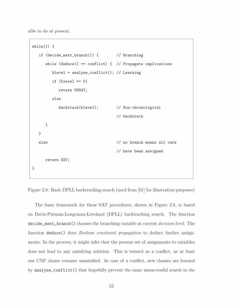
able to do at present.

while(1) {

if (decide_next_branch()) { // Branching

while (deduce() == conflict) { // Propagate implications

blevel = analyse_conflict(); // Learning

if (blevel == 0)

return UNSAT;

else

backtrack(blevel); // Non-chronological

// backtrack

}

}

else // no branch means all vars

// have been assigned

return SAT;

}

Figure 2.8: Basic DPLL backtracking search (used from [61] for illustration purposes)

The basic framework for these SAT procedures, shown in Figure 2.8, is based

on Davis-Putnam-Longeman-Loveland (DPLL) backtracking search. The function

decide_next_branch() chooses the branching variable at current decision level. The

function deduce() does Boolean constraint propagation to deduce further assign-

ments. In the process, it might infer that the present set of assignments to variables

does not lead to any satisfying solution. This is termed as a conflict, as at least

one CNF clause remains unsatisfied. In case of a conflict, new clauses are learned

by analyze_conflict() that hopefully prevent the same unsuccessful search in the

52

future. The conflict analysis also returns a variable for which another value should

be tried. This variable may not be the most recent variable decided, leading to a

non-chronological backtrack. If all variables have been decided, then we have found

a satisfying assignment and the procedure returns. The strength of various SAT

checkers lies in their implementation of constraint propagation, non-chronological

backtracking, decision heuristics, and learning.

Modern SAT checkers work by introducing conflict clauses in the learning phase

and by non-chronological backtracking. Implication graphs are used for Boolean con-

straint propagation. The vertexes of this graph are literals, and each edge is labeled

with the clause that forces the assignment. When a clause becomes unsatisfiable as a

result of the current set of assignments (decision assignments or implied assignments),

a conflict clause is introduced to record the cause of the conflict, so that the same

futile search is never repeated. The conflict clause is learned from the structure of

the implication graph. When the search backtracks, it backtracks to the most recent

variable in the conflict clause just added, not to the variable that was assigned last.

In our enumeration algorithm, we use the Chaff SAT checker [61], as it has been

demonstrated to be the most powerful SAT checker on a wide class of problems.

2.5 SAT Procedures for Reachability Analysis

Following the outline of the basic reachability algorithm 2.1, we can use SAT pro-

cedures for image computation. The transition relation and the set of states is rep-

resented using a propositional formulas. SAT checkers like Chaff read propositional

formulas represented in conjunctive normal forms (CNFs). We present an algorithm

that does not use any BDDs. We assume that the transition relation T (x, i,x′) is al-

ready represented in as a set of CNF clauses. It is customary to convert any transition

53

relation represented as a set of propositional formula to CNF form by introducing in-

termediate variables. This translation is polynomial in the size of the original circuit.

We represent the set of newly reached states after each iteration of the reachability

loop (Si in Figure 2.1) as a set of disjunctive normal form (DNF) cubes. The set of all

reachable states after each step (Sreach) is also represented in DNF. Since Sreach is in

DNF, ¬Sreach will be automatically in CNF. As Chaff needs CNF representation, we

convert Si from DNF to CNF by introducing intermediate variables. In each iteration

i, we ask the SAT checker to find satisfying assignments to the formula below.

Si−1(x) ∧ T (x, i,x′) ∧ ¬Sreach(x′) (2.7)

Formula 2.7 corresponds to step 5 of the basic reachability algorithm (Fig. 2.1).

Any satisfying assignment to Formula 2.7 is such that the present state variables x

and input variables i satisfy the predicate Si−1(x) ∧ T (x, i,x′), i. e., the set of states

reachable from the newly discovered states in the previous iteration. Furthermore,

such a satisfying assignment also is in the negation of the set of all accumulated states

so far (¬Sreach), thus we ask the SAT checker to compute only the states that have

not been seen so far. If the SAT checker concludes that the formula is unsatisfiable,

then it means that the set of newly reached states Si is empty, and we have reached

fixed-point. On the other hand, if the SAT checker finds a satisfying assignment to

this formula in present state x, input i, intermediate and x′ variables, the projection

of this assignment on x′ variables gives a subset of newly reached states. Note that

this partial assignment to x′ is consistent with the full assignment that the SAT

checker finds to the Formula 2.7. The Formula 2.7 describes all constraints on the

next set of states. Therefore, the projection is a valid state reachable from Si−1

following the transition relation T . Thus, the following lemma easily follows.

54

/* It is assumed that S0 is given in DNF form */

SatReachability(S0)

1 i← 1

2 Sreach ← S0

3 while (Si−1 6= φ)

4 Si ← φ

/* DNFtoCNF converts a formula to CNF by

introducing intermediate variables */

5 for (each satisfying partial assignment d in x′ to

DNFtoCNF (Si−1(x)) ∧ T (x, i,x′) ∧ ¬Sreach(x′))

/* d contains only next state variables */

6 d′ ← EnlargeCube(d)

7 Add ¬d′ as a blocking clause

8 Si ← AddCube(Si, next2current(d′))

9 Sreach ← AddCube(Sreach,d′)

10 endfor

11 endwhile

12 return next2current(Sreach)

Figure 2.9: Outline of the SAT based reachability algorithm

55

Lemma 1 The projection of any partial satisfying assignment to Equation 2.7 in x,

i, x′ and intermediate variables to just x′ is a valid partial assignment in x′ describing

a newly discovered state reachable from Si−1 following T .

We add this state to Si(x) as a DNF cube d, after translating the next state

variables in the cube to present state variables. The negation of d is a CNF clause,

which is added as a conflict clause in the SAT engine. This clause ¬d is called

a blocking clause. Thus after finding each satisfying assignment, the set Sreach(x′)

grows.

We present the high level algorithm in Figure 2.9. The algorithm has two loops.

The outer loop carries out different steps of image computation, while the inner loop

is implicit in the SAT checker, and enumerates sets of the newly reached states in a

particular step.

Each satisfying cube d is added to Si and Sreach after enlarging it to d′ in step

6. The addition of d′ to Sreach is done in the SAT checker when the blocking clause

¬d′ is added. As noted earlier, negation of Sreach is automatically in CNF. Step 6

of the algorithm is crucial to make our approach efficient and practical. We describe

the efficiency issues, including step 6 of the algorithm, in the next subsection.

2.5.1 Efficient Implementation of SAT Based Reachability

Algorithm given in Figure 2.9, without step 6, is very inefficient and hence imprac-

tical. The first problem comes from the way the SAT checker computes satisfying

assignments or cubes. The Chaff SAT checker gives values to all variables in any

assignment. We then project this assignment to d, which assigns values to all next

state variables x′. Therefore d describes only one newly reached state. Enumerating

states one at a time is clearly very inefficient. However, most of the times, one does

56

not need to come up with a complete assignment to satisfy the CNF formula. A par-

tial assignment to x′ describes more than one state at a time, the larger the set, the

fewer the number of assignments. This is advantageous in two ways, first the block-

ing clause for d prunes the SAT search space drastically, second, the number of state

enumerations required go down considerably. Therefore, it is desired that the partial

assignment be as small as possible. It is clearly to our advantage to get as small cubes

as possible, since smaller cubes cover a larger number of assignments. Given a cube

computed by Chaff, it may be possible to throw away certain assignments from the

cube, and still get a satisfying cube. By a static analysis of the transition relation,

we infer the unnecessary assignments in d. This procedure EnlargeCube, described

in the next sub-section, is called in line 6 on d to get a smaller cube d′.

The second problem is that the representation of the sets Sreach and even Si can

grow too large. For example, if we consider a counter that counts up to 230, each

iteration of the while loop will add only one state to Sreach. Thus we will have to

represent 230 clauses for Sreach. However, the DNF clause 1 represents all possible

values of the counter. In other words, after a satisfying assignment to Sreach is found,

we can combine multiple clauses to get a smaller partial assignment. For example,

the DNF clauses x1 ∧ x5 ∧ ¬x6 and x1 ∧ x5 ∧ x6 can be combined to x1 ∧ x5. An

efficient data structure is needed to support this AddClause operation, since many

clauses may be added, and each clause can potentially be combined with more than

one existing clause. We use a hash table, each entry of which contains a trie [47].

We give a cube enlargement heuristic procedure next, which is followed by a

description of an efficient data structure that stores Si and Sreach. The enlargement

procedure reduces the number of enumerations, hence reducesthe amount of time,

while the second procedure reduces the space requirement.

57

2.5.2 Cube Enlargement

There are five types of variables that appear in the SAT formula 2.7: present state

variables x, circuit inputs i, next state variables x′, intermediate variables is intro-

duced while converting Si−1 to CNF, and the intermediate variables it introduced

while converting the transition relation T (x, i,x′) to CNF. The SAT checker finds

a satisfying assignment c, possibly to all these variables. However, the cube d of

line 7 in the algorithm (Fig. 2.9) is just in terms of x′ variables. In order to reduce

the number of assignments in d, we use the following procedure. This procedure as-

sumes that the transition relation is given in functional form, i.e., there is a transition

function fi(x) for each next state variables xi. This assumption is true for circuit

descriptions. Let Supp(fi) denote the support set of fi, i.e., the variables that fi

depends on. When an assignment to a next state variable x′i can be ignored, we say

that x′i is *.

Free Variables

First, we describe the concept of free variables, i.e., the variables that are free to

assume any value, despite the SAT checker assigning them specific values. In other

words, we can ignore any assignment by the SAT checker to free variables. In order to

detect whether the variable v is free or not, the following conservative tests are used. If

v is an input variable or an intermediate variable, then it is definitely free. Moreover,

for functional transition relations, we don’t even need to check if an intermediate

variable appears in other transition functions or not, since intermediate variables are

generated from the local translation for fi. The only real problem arises when v is

a present state variable. The only constraints that are placed on the present state

variables are from Si−1. To see if the present satisfying assignment c restricts v or

58

not, we can just check that the assignment to v does not affect the present satisfying

assignment. This can be efficiently detected as follows. While translating the DNF

corresponding to Si−1 to CNF, we introduce one intermediate variable for each DNF

cube. In essence, the truth value of each DNF cube is captured in the corresponding

variable. Suppose i1, i2, . . . , ik are the intermediate variables corresponding to DNF

cubes D1, D2, . . . , Dk in Si−1. The translation of the Si−1 constraint in Eqn. 2.7 looks

like:

(i1 ∨ i2 ∨ . . . ∨ ik) ∧ (i1 ⇔ D1) ∧ (i2 ⇔ D2) ∧ . . . ∧ (ik ⇔ Dk) (2.8)

Each equality ij ⇔ Dj gives rise to a set of CNF clauses, which we haven’t expanded

for the sake of brevity.

If the satisfying assignment c makes any of the intermediate variables true, the

corresponding DNF cube is true, and we don’t need to see if any other DNF cube

is true, since the truth of only one DNF cube satisfies the Si−1 clauses. So we find

the first intermediate variable il that is set to true. All present state variables not

mentioned in the DNF cube Dl are irrelevant for satisfying the constraint Si−1, hence,

they can be assumed to be free.

Free Transition Functions

Let us denote the set of free variables in the support of a transition function fi by

FreeSupp(fi).

The main idea is that if a transition function fi (for x′i) depends on a variable v

(which is either a present state variable, input or an intermediate variable from it),

and the following conditions are satisfied, then we can guarantee that x′i can assume

any value. Thus, the value of x′i can be safely ignored from the present assignment.

1. Variable v is free.

59

2. After propagating the values of non-free variables in Supp(fi), fi is not forced

to a particular value. For example, suppose that fi = x1 ∧ x2, x1 is free, and

x2 = 0 in Si−1. Propagating the value of x2 forces fi to 0. Thus, constant

values of non-free variables are propagated first to detect such scenarios.

3. The function fi does not share free support with any other transition function,

i.e., FreeSupp(fi)∩FreeSupp(fj) = φ, j 6= i. Moreover, the variable v appears

in the formula for fi in exactly one place.

Note that there may be other conditions under which x′i can still choose both

values. However, the conditions presented above allow us to do a static analysis of

the circuit.

The third condition is too restrictive in practice. Usually, transition functions do

share common variables. In order to infer that a next state variable x′i can assume

both values, we can simplify the transition functions by further constant-propagating

values of some free variables as well (remember that we already constant-propagate

the values of non-free variables). For example, suppose that f1 = x1 ∨ i2 and f2 =

x1 ∨ i3, and x1, i1 and i3 are free variables. Suppose the SAT assignment is x1 =

0, i1 = 0, i2 = 1. Since both f1 and f2 share the variable x1, we can not safely say

that both x′1 and x′

2 are *. However, we can replace x1 by 0, and propagate the effects,

giving us f1 = i2 and f2 = i3. Now, both f1 and f2 become independent, and can be

set to *. Note that since x1 is a free variable, we could have chosen x1 = 1, different

from the SAT assignment. In order to determine the set of variables to assign values

to, such that the transition functions become independent, we use a greedy strategy.

We order the variables by the number of times they appear in all transition functions.

Beginning with the variable that occurs the most number of times, we keep replacing

the variables by constants (from SAT assignment) and propagating the effect, until

60

transition functions become independent and next state variables can be inferred to

be *s. In the worst case, all transition functions become constants.

Most analysis of this procedure can be done statically just once. The only chang-

ing part is detection of free present state variables. Note that the process described

above is just one alternative for cube enlargement. There can be other options. For

example, we considered using efficient approximate set cover algorithms to find out

the literals that cover all clauses of formula 2.7. Another option is to use BDD based

symbolic simulation to infer multiple cubes. The given cube enlargement procedure

produces one smaller cube. However, using BDDs for simulation of the circuit for

one step and then applying constants to some of BDD variables to contain the BDD

sizes can yield a set of many states at once.

2.5.3 Efficient Set Representation

The set of states are represented as a set of DNF cubes. However, it is easy to see

that each new cube that is added to Sreach has a potential to be merged with other

cubes to form shorter cubes. For example, the boolean function 1 is an exponentially

more compact representation than four DNF cubes a ∧ b,¬a ∧ b, a ∧ ¬b,¬a ∧ ¬b.

We describe the following procedure to add a cube to the existing set of cubes. We

assume that the variables in the cubes are ordered. The set is represented by a hash

table, where each hash table entry stores a subset of cubes in the trie, or a prefix tree

data structure. Tries are often used to store dictionaries efficiently. Knuth’s volume

3 on sorting and searching provides a good description of tries. In our case, each

trie stores cubes that are made up of the same CNF variables. The hash table is

indexed by the hash computed from a signature of a cube. In the following algorithm

(Figure 2.11), assume that the DNF cube d is represented as a vector of integers,

each integer identifying a particular propositional variable, negative if the literal is

61

negative, positive otherwise. For example, if a, b, c, d, e, f... are variables, then they

are identified by the integers 1, 2, 3, 4, 5, 6, .... So a cube (a ∧ ¬c ∧ ¬f) is represented

by the vector d = [1,−3,−6]. The function ComputeSignature computes a bit

string that is used to compute the hash value for a cube. The bit string is ordered,

just as variables in the cubes are, and contains 1 for each variable present and 0 for

the variables not present in the cube. The trailing 0s are removed to get a shorter

bit string. Thus even though there may be variables numbered 7, 8, 9, .., the 0s

corresponding to them do not appear in the signature. So the signature for the cube

d is 101001.

ComputeSignature(d,m)

/* m is the size of the cube d, assume d is sorted */

1 j ← 1

2 for (i from 1 to d[m])

3 if (i = |d[j]|) /* variable is present in d */

4 sd[i]← 1

5 j ← j + 1

else

6 sd[i]← 0

endif

endfor

7 return sd

Figure 2.10: Procedure ComputeSignature.

Since each trie stores cubes made up of the same variables, the cubes are repre-

sented by bit strings of the same length as the number of variables in the cubes of

the trie. Essentially, if a literal is positive, the bit corresponding to it is 1, and 0

62

otherwise. So the cube d is stored as 100.

The crux of the AddCube procedure is between lines 5–19. Given an incoming

cube d, it tries to find all other cubes from the trie that differ from d in just one bit.

For each such cube d′ found (lines 10–13), the cube computed by merging d and d′

is added to S by calling AddCube recursively. The merged cube is essentially cube

d with the matched bit (ith bit) removed. If d doesn’t match at the ith bit, then

the next bit is checked. Once the traversal over the trie is done, we check if d was

merged with anything. If it was, then we no longer keep d. Line 18 just updates the

hash table with potentially modified trie.

Note that the algorithm doesn’t guarantee absolute minimum cubes. In fact, to

do so, we may need to keep all cubes, even after they are merged, in the hopes of

merging them with other future cubes. But the main focus of the algorithm is to

reduce space, and not get the absolute smallest cubes. Another point to note is that

since the SAT checker always finds new states that haven’t been discovered so far,

we assume that the trie Td does not already contain d.

The complexity of this algorithm in the worst case can be O(n2). Here n is the

number of state variables. Each of line 1, 3–4, 6 and 17 cost O(n), while hash lookups

and updates on lines 2 and 18 are essentially constant time operations. Lines 10 and

11 cost O(m) + O(m− 1) + . . . + O(1) = O(m2) = O(n2).

2.5.4 Complexity of the Set Representation

The set of DNF cubes representing Si or Sreach possess a useful property. By the

negation of Sreach in the SAT formula (Eqn. 2.7), we guarantee that no newly gen-

erated DNF cube shares a satisfying assignment with any existing cube in sets Si or

Sreach. Thus the set of DNF cubes representing these sets are disjoint, in that they

63

AddCube(S, d, n, m)

/* n is the total number of variables, m is the number of variables in d */

1 sd ← ComputeSignature(d,m)

2 Td ← HashLookup(S, sd) /* Td is the trie in which d will be stored */

/* compute the representation of d to store in Td */

3 for (i from 1 to m)

4 b[i]← (d[i] > 0)?1 : 0

5 match← false

6 Td ← TrieInsert(Td,b)

7 curr node← Td

8 for (i from 1 to m)

9 b[i]← 1− b[i] /* flip the ith bit */

10 if (TrieLookup(curr node,b[i : m]) = true)

11 Td ← TrieDelete(Td,b) /* match at the ith bit */

/* insert the merged cube */

12 S ← AddCube(S,d[1 : i− 1] :: d[i + 1 : m], n,m)

13 match← true

endif

14 b[i]← 1− b[i] /* flip it back to what it was */

15 curr node← (b[i] = 1)?curr node.right : curr node.left

endfor

16 if (match = true)

17 Td ← TrieDelete(Td,b)

18 S ← HashUpdate(S, sd, Td) /* update the trie for this cube */

19 return S

Figure 2.11: Procedures AddCube.

64

do not have any common assignment. For example, the DNF cube b ∧ c ∧ d cannot

occur if the cube a ∧ b ∧ c is already present, as they share a common assignment

a = b = c = d = 1. However, cube ¬a ∧ b ∧ c ∧ d can occur. If we can detect that

the set of cubes is a tautology, we can terminate the reachability, as we have reached

all the states. Our cube addition algorithm is online in nature. We now prove that

if the set of DNF cubes that do not share a common satisfying assignment is given

a priori, then detecting if it is a tautology is polynomial. The general problem of

detecting DNF tautology is coNP-complete.

Let us call the problem of tautology detection of a set of DNF cubes that do not

share any pair wise common assignment an R-TAUT problem. The procedure for

tautology detection works simply by counting the number of satisfying assignments.

Suppose that there are c DNF cubes made up from a total of m variables, and that

the cubes do not share common assignments pair wise. Suppose cube i has literals

l1, l2, . . . , lci. There are a total of 2m possible assignments to variables, and if each

assignment is a satisfying assignment, then the DNF cubes are a tautology. Cube

i describes a total of 2m−ci assignments agreeing with the literals in cube i. As we

know that no two cubes i and j share any common assignment, the total number of

assignments that satisfy both cube i and j are precisely 2m−ci + 2m−cj . The total

number of satisfying assignments for the set of DNF cubes is just

2m−c1 + 2m−c2 + . . . + 2m−cc .

Clearly, the additions can be carried out in time polynomial in m and c, the size of

problem input. Hence the theorem

Theorem 2 R-TAUT is in P.

Note that in our case, the set of DNF cubes are not given a priori. However, this

procedure can be run periodically on Sreach to find out if all states have been reached,

65

in which case we stop the search. We also use this counting mechanism to report the

number of reached states.

2.6 Results for SAT Based Reachability Analysis

We implemented our algorithms on top of the zChaff SAT solver. The SAT solver is

modified to enumerate satisfying solutions by adding blocking clauses.

We conducted our experiments on a 1.53GHz dual AMD Athlon processor ma-

chine with 3GB of memory running Linux. The memory cutoff was set to 1.5GB

of resident program size, and the time cut off was set to 1000 seconds. The results

are summarized in table 2.5. For each circuit, we report the number of latches, the

number of reachability steps that we could complete, the number of cubes stored in

the representation for the reachable states, the number of cubes that were enumer-

ated as blocking clauses (or how many times line 7 in algorithm of Figure 2.9 was

called), the ratio of the number cubes v/s the number of blocking clauses added in

percentage, and the total running time (user time+system time) in seconds. Note

that the number of cubes in the final set representation is much smaller than the

total number of enumerated cubes, as evidenced by the %age size column, asserting

that the space saving data structure for storing cubes is effective. We compare our

results with primarily that of [57]. We would like to emphasize that in [57], only the

depth was computed, and the actual set of reachable states was not computed.

The circuits that we report come from mainly three sources, ISCAS’89 bench-

marks, IU set of circuits from Synopsys, and some circuits that were translated from

Verilog code available from various sources. The IU set of circuits are various ab-

stractions of parts of a picoJava microprocessor implementation.

For a relatively small timeout value, we have been able to do reachability for many

66

Circuit # latches # steps Space Requirement Time (sec) Comparison with [57]

# cubes # blocking clauses %age space Max. Depth Time (sec)

decss 86 85* 655 131304 0.50 1000.00

iu30 30 4* 3343 72037 4.64 1000.00

iu35 35 3* 1479 94424 1.57 1000.00

iu40 40 2* 20 33168 0.06 1000.00

iu45 45 1* 2294 165192 1.39 1000.00

s208.1 8 255 8 255 3.14 0.56

s298 14 18 33 217 15.21 0.33 18 19.3

s344 15 6 558 2624 21.27 15.30

s349 15 6 546 2624 20.81 14.82

s382 21 150 337 8864 3.80 7.71

s386 6 7 6 12 50.00 0.21 7 0.18

s400 21 150 336 8864 3.79 7.81

s420.1 16 65535 16 65535 0.02 213.97

s444 21 150 341 8864 3.85 8.00

s499 22 21 21 21 100.00 1.74 21 1.07

s510 6 46 10 46 21.74 0.47 46 144.81

s526 21 150 381 8867 4.30 9.35

s526n 21 150 372 8867 4.20 9.21

s635 32 125528* 66 125528 0.05 1000.00

s641 19 6 321 1543 20.80 2.24 6 97.03

s713 19 6 363 1543 23.53 2.53 6 126.94

s820 5 10 11 24 45.83 0.48 10 2.51

s832 5 10 11 24 45.83 0.47

s838.1 32 155441* 26 155441 0.02 1000.00

s953 29 10 189 503 37.57 2.01 10 102.23

s967 29 10 177 548 32.30 3.12

s1196 18 2 802 2615 30.67 6.79 2 232.84

s1238 18 2 849 2615 32.47 7.26

s1269 37 1* 2136 4339 49.23 1000.00 7* 5000

s1423 74 3* 2652 55568 4.77 1000.00 26* 5000

s1488 6 21 19 47 40.43 0.87 21 96.87

s1494 6 21 19 47 40.43 0.87

s1512 57 4* 2035 178175 1.14 1000.00

s9234 228 8* 507 6651 7.62 1000.00

s13207 669 2* 76 1824 4.17 1000.00

s15850 597 5* 362 2558 14.15 1000.00

s38584 1452 2* 58 452 12.83 1000.00

Table 2.5: Experimental results on a set of circuits from various sources including ISCAS’89 and Synopsys. The comparison

is against [57]. Note: (*)-reachability was not complete. Empty boxes denote results N/A.

67

circuits. Our technique outperformed the one in [57] by a large magnitude on all but

one small completed benchmarks. The authors of [57] used a faster machine (2GHz

v/s 1.53GHz) as well. The effectiveness of the cube merging procedure is evident from

“%age space” column. The savings are dramatic for circuits that have counter-like

structures in them (iu**, s208.1, s420.1, s838.1, s635), and also for some circuits that

are not known to have counters (s1512, s9234, s13207, s1423, s526, s526n). For other

circuits, it can be inferred that the SAT checker and cube enlargement procedures

generate many disjoint cubes that can not be merged with the existing set of cubes.

This may be dependent on circuit structure.

Lahiri et al. [50] used our tool to enumerate symbolic solutions to certain predicate

abstraction formulas. The characteristic of these formulas was that the number of

variables to be quantified was much larger (an order of magnitude) than the number

of variables representing the set of states. For image computation, the number of

variables to be quantified may not necessarily be much larger than the number of

state variables.

2.7 Related Work

Burch et al. [12] and Touati et al. [70] first recognized the importance of early quan-

tification for image computation. Geist and Beer [33] proposed a simple heuristic

algorithm, in which they ordered conjuncts in the increasing order of the number of

support variables. Touati et al. were the first to formulate the early quantification

problem as an evaluation of a parse tree and proved the NP-completeness of the prob-

lem. They also offered a greedy strategy for evaluation of the parse tree by evaluating

the node with the smallest support set next. However, they do not compare their

technique against other techniques, so the effectiveness of their algorithms was not

68

clear. All successful techniques so far in the literature consider only linear conjunc-

tion schedules and use the same conjunction schedule for all the image computations

during symbolic analysis. These techniques begin by first ordering the conjuncts and

then clustering them and finally ordering the clusters again using the same heuris-

tics. Ranjan et al. [64] proposed the first successful heuristics for this problem and

Yang [73] refined their technique. The ordering procedures of both papers linearly

orders the BDDs based on a heuristic score. The individual BDDs are then formed

into clusters by conjoining them according to the order until BDD size grows beyond

certain threshold. Finally, these clusters are ordered using the same algorithm. A

recent paper by Moon and Somenzi [60] presents an ordering algorithm (henceforth

referred to as FMCAD00) based on computing the Bordered Block Triangular form

of the dependence matrix to minimize the average active lifetime of variables. Their

clustering algorithm is based on the sharing of support variables (affinity). We ex-

tended their notion of lifetimes and used combinatorial algorithms to improve the

performance [16].

The first completely SAT based reachability algorithm was reported by McMillan

in [53]. The main difference between our SAT based reachability algorithm is that we

represent the set of states in DNF, while he represented the set of states in CNF. A

SAT based enumeration algorithm is used to compute a CNF formula equivalent to

a given formula characterizing preimages. However, we use intermediate variables to

convert the DNF representation to CNF while running SAT. He used zero suppressed

BDDs (zDDs) to store the CNF clauses, and used a SAT conflict analysis based

heuristic to enlarge the cubes. We did not compare the results reported in [53] as

the set of benchmarks in [53] was not publicly available.

In [44], the authors used a procedure similar to our SAT based reachability to

compute preimages. They also use intermediate variables to convert DNF cubes to

69

CNF formulas. However, they use the offline version of the Espresso [65] algorithm

to reduce the number of cubes. Our cube storage procedure is on-line, in the sense

that it processes the cubes as they are generated. Moreover, they do not have any

algorithm to enlarge the cubes. They also reported the results only on two different

circuits and for safety property checking only, which can be much easier than to do

than reachability when the property is false. Our attempts to contact them to get

more information about the properties they checked failed.

In [68], the authors used ATPG instead of SAT to compute preimages. They used

BDDS to store the resultant sets of states. ATPG allows reasoning directly on the

circuits, hence they do not have any intermediate variables. They report results on

only two circuits. These are known to be difficult circuits, however.

In [57], the only aim is to compute the sequential diameter, also called the di-

ameter of the circuit. They do not compute the reachable set of states at all. Their

procedure is based on the Chaff SAT checker as ours is. Their procedures shares many

similarities with bounded model checking (BMC) [5]. They build a SAT formula de-

scribing symbolic simulations of increasing length. In our SAT based reachability

approach, we explicitly compute the set of reachable states, and the SAT checker

does not have to compute more than one step of symbolic simulation at a time. We

believe that this is a significant advantage that our method has over [57] and BMC.

Using BMC for depth equal to circuit diameter is sufficient for Gp kind of LTL

properties. In [48], this notion is generalized to that of completeness threshold (CT).

The authors describe a sorting network built on top of SAT formula for computing

diameters.

In [38, 39], a mixed BDD and SAT based approach to image computation is

described. They use SAT procedure to derive a top level disjunctive decomposition of

image computation and use BDD based image computation for each leaf subproblem.

70

2.8 Summary

We have proposed simple yet effective quantification scheduling algorithms for the

image computation problem. We view the problem of quantification scheduling for

symbolic image computation as a quantified Boolean formula evaluation problem. We

have also proposed heuristic algorithms based on scoring of quantification variables

to reduce the size of the intermediate BDDs. We have demonstrated that our simple

yet flexible approach yields better experimental results for many reachability analysis

and model checking problems.

We can view the problem of building an optimal parse tree as a combinatorial

optimization problem and apply techniques like simulated annealing to get better

quantification schedules. A middle ground between dynamic and static techniques

seems promising. For example, we believe that beginning with some static schedule,

the schedule can be tuned for a particular image computation with a little effort.

We also want to investigate techniques of approximating sizes of BDDs based on

the size of support sets, which will definitely improve all image computation heuris-

tics. The techniques developed for quantification scheduling can be applied to other

related problems, like splitting orders in SAT checkers [7] and hierarchical model

checking [58].

Moving on to SAT, we presented a completely SAT based image computation al-

gorithm. The effectiveness of this algorithm is demonstrated for reachability analysis

on many large circuits. This algorithm can be used for computing pre images equally

well, hence it can be used in a general SAT based symbolic model checking algo-

rithm. The novel features of our algorithm are an efficient data structure for storing

sets of states as DNF cubes and a cube enlargement procedure based on static circuit

analysis.

71

72

Chapter 3

SAT Based Reparameterization

Algorithm for Symbolic Simulation

3.1 Introduction

Symbolic simulation is a widely applied technique for analysis of complex transition

systems and synchronous circuits in particular. In symbolic simulation, the transition

relation is unwound m times into an equation that represents the set of states that is

reachable in exactly m steps. The simulator keeps separate equations for each state

variable. They are parameterized in the initial state and the inputs of the circuit.

Thus, the set of states is stored in a parametric representation.

An efficient way to store and manipulate this parametric representation of the

set of states is crucial for the performance of the algorithm. Such a representation

describes a set of states as a vector (f1, f2, . . . , fn) of functions in parameters P =

{p1, p2, . . . , pm}. Each parametric function gives the value of one state variable. For

example, the set of states S = {10, 01} is represented parametrically as (p1,¬p1). In

this case, there is only one parameter p1.

73

Most implementations use BDDs to represent these functions [1, 30, 34, 35, 43,

74]. These BDDs may grow exponentially in the number of simulation steps, as the

number of variables grows. In order to address this problem, symbolic simulators

compute a new, equivalent parametric representation. The new representation can

be significantly smaller since it usually requires much fewer variables. This step is

done as soon as one of the BDDs becomes too large. The process of converting one

parametric representation to another is called reparameterization. In [30] and [43],

the reparameterization algorithm first converts the parametric representation into

characteristic function form and then parameterizes this form. In [34], an algorithm is

given for computing set union in parametric form. Algorithms for reparameterization

and quantification are given that are based on this set union algorithm. However,

the reparameterization is done using BDDs, hence as the number of simulation steps

grows, the algorithm quickly becomes very expensive. This is due to the fact that

each simulation step introduces more input variables, which need to be quantified

during reparameterization.

Novel Contributions We describe a SAT-based algorithm to perform the repa-

rameterization step for symbolic simulation. The algorithm performs better than

BDD-based reparameterization especially in the presence of many input variables.

The algorithm takes arbitrary Boolean equations as input. Therefore, it does not

require BDDs for the symbolic simulation. Thus, symbolic simulation can benefit

from non-canonical forms that grow at most linearly with the number of simulation

steps.

In essence, the SAT-based reparameterization algorithm computes a new para-

metric function for each state variable one at a time. In each computation, a large

number of input variables are quantified by a single call to a SAT-based enumera-

74

tion procedure, e.g. [18,53], described in Chapter 2. The advantage of this approach

is twofold: First, all input variables are quantified at the same time, and second,

the performance of SAT-based enumeration procedure is largely unaffected by the

number of input variables that are quantified.

We demonstrate the efficiency of this new technique using large industrial circuits

with thousands of latches. We compare it to both SAT-based Bounded Model Check-

ing and BDD-based symbolic simulation. Our new algorithm can go much deeper

than a standard Bounded Model Checker can. Moreover, the overall memory con-

sumption and the run times are, on average, 3 times less than the values measured

using a Bounded Model Checker. The BDD-based symbolic simulator could not even

verify most of the circuits that we used.

3.2 Parametric Representation

Characteristic functions and parametric representations are two well known methods

of representing a set of Boolean vectors. A set of Boolean vectors over the state

variables represents a set of states. Consider a set S of vectors over the variables

V = {v1, v2, . . . , vn}. As described above, v = (v1, v2, . . . , vn) denotes a particular

vector or a particular assignments to the variables in V . If the characteristic function

ξ(v) represents the set S of vectors, then

S = {v ∈ Sn | ξ(v) = 1}. (3.1)

Example The following example will be used throughout this chapter. Let v1

and v2 be two Boolean state variables. Consider the set of states {01, 10, 11}. A

characteristic function for this set of states is ξ(v) = v1 ∨ v2.

On the other hand, if S is represented parametrically with a vector of n functions

75

f(p) = (f1(p), f2(p), . . . , fn(p)) over m parameters p = (p1, p2, . . . , pm), then

S = {v ∈ Sn | ∃p ∈ Pm[v1 = f1(p) ∧ v2 = f2(p) ∧ . . . ∧ vn = fn(p)]}. (3.2)

Informally, the set of vectors in S is given by the range of the vector of functions

(f1(p), f2(p), . . . , fn(p)), where p ranges over all possible Boolean vectors in Pm. For

the running example, one possible parametric representation with three parameters

P = {p1, p2, p3} is

(f1(p) = p1 ∧ p2, f2(p) = ¬(p1 ∧ p2) ∨ p3).

Note that, in general, m 6= n. For the particular case of symbolic simulation that

we will discuss later, the number of parameters will be equal to the number of input

variables to the circuit times the number of simulation steps, which can be much

larger than n.

A parametric representation can be easily converted to a characteristic function

by using the following equation:

ξ(v) = ∃p[(v1 ↔ f1(p)) ∧ (v2 ↔ f2(p)) ∧ . . . ∧ (vn ↔ fn(p))]. (3.3)

In other words, ξ(v) is true if the there exists an assignment p to the parameters

such that the parametric function f1(p) evaluates to v1, f2(p) evaluates v2, and so on.

This is what is desired, since ξ is supposed to be true exactly for the vectors in the

set. In the case of symbolic simulation, p consists of the initial state and the inputs

on the path to the state ξ(v).

Note that the conversion to characteristic function involves Boolean quantification

over the parameters. If the functions are represented by BDDs, then this quantifi-

cation becomes harder as the number of parameters m and the number of state

variables n increase. As we have seen in chapter 2, a similar quantification problem

76

occurs in BDD-based image computation when a transition relation is represented in

conjunctively decomposed form. In that case, the variables to be quantified are the

present state and input variables of the circuit, while the next state variables are not

quantified.

Before proceeding further, we describe the notations and conventions we will use

in this chapter.

Notations and Conventions

Sets will be denoted by capital letters, as in S for the set of states, V for the set

of state variables, Ik for the set of input variables, and P for the set of parametric

variables. We use a superscript of k for input variables to denote input variables

accumulated over k steps of symbolic simulation. An ordered tuple of lower case

letters denotes a vector of variables. For example, the state variable vector with n

state variables is (v1, v2, . . . , vn). A vector is denoted by using a bar over the symbol.

For example, a state vector will be denoted by v, an input vector of variables from

Ik is denoted by ι. Similarly, a parameter vector is denoted by p = (p1, p2, . . . , pm).

The set of all possible 2n vectors of n state variables is Sn, the set of all possible 2m

assignments to m parameters is Pm, and the set of all possible input vectors is Wk.

Other uppercase calligraphic letters denote subsets of these sets. When the number

of components in a vector is clear, we will often drop the subscripts, and just use

S,P , and so on. Functions will be denoted by lower case symbols, e.g., f(ι). In

the parenthesis after a function symbol, the list of variables on which the function

depends (the support set) is given, e.g., h1i (p1, p2, . . . , pi). A vector of functions will

be denoted by a bar over the top of the function symbol. For example, a vector of

parametric functions is h(p) = (h1(p), h2(p), . . . , hn(p)). The symbol α will denote

the constants 0 or 1. We sometimes use the symbol t(j) to denote the state vector

77

at step j of the simulation in the trace t(0), . . . , t(k) of length k.

We summarize this notation in the following Table 3.1.

n : number of state variables

m : number of parameters

l, k : number of simulation steps

Sets of Variables Vectors of Variables Sets of Vectors

V = {v1, v2, . . . , vn} :

state variables

v = (v1, v2, . . . , vn) :

state variable vector

Sn or S : set of all state

vectors

Xn,Yn or X ,Y : subsets

of Sn

P = {p1, p2, . . . , pm} :

parameters

p = (p1, p2, . . . , pm) : pa-

rameter vector

Pm or P : set of all pa-

rameter vectors

Ik : all inputs from step

1 to kιk or ι : input vector

Wk : all input vectors

J k,Kk : subsets of Wk

Functions Vectors of Functions

fi(ι) : simulated expression for state

variable vi

f(ι) = (f1(ι), f2(ι), . . . , fn(ι)) : vector

of simulated expressions for all state

variables

hi(p) : parametric function for vi

h(p) = (h1(p), h2(p), . . . , hn(p)) : vector

of parametric functions

Table 3.1: Notations and Conventions.

Parametric Representation in Symbolic Simulation

Consider a circuit C with p inputs and n state variables. Suppose the circuit is

symbolically simulated for k steps, by building Boolean expressions that represent

78

the values of each of the state bits. After the k-step simulation, suppose each state

bit vi is given by a Boolean expression denoted by the function fi(ι). The variables Ik

appearing in each function fi(ι) are the p·k inputs plus the n initial values of the state

variables. Thus, |Ik| = m = p · k + n. We will denote the set of input vectors over Ik

variables by Wk and a particular input vector by ι. Traditional symbolic simulators

can simulate a large number of steps, making p · k ≫ n. The set of reachable states

in k steps, as a set of state vectors in V variables, is given by

S = {v ∈ Sn | ∃ι ∈ Wk[v1 = f1(ι) ∧ v2 = f2(ι) ∧ . . . ∧ vn = fn(ι)]}.

Thus symbolic simulation builds a parametric representation of the set of states

reachable in exactly k steps, where the parameters are input variables Ik.

Usually, the number of parameters |Ik| is very large. The number of possible

valuations of these variables is 2|Ik|, while the number of possible valuations of the

state variables is 2n. Therefore, many vectors in Wk variables will map to the same

state vector. Hence, it should be possible to reduce the number of parameters. We

aim at finding new functions h1(p), h2(p), . . . , hn(p) in new parameters P , where

|P | ≪ |Ik|. This is why reparameterization is useful. Obviously, a set of vectors in n

variables can be represented by parametric functions of n variables. Hence, |P | ≤ n.

This process of converting from one parametric representation to another is called

reparameterization [30, 34].

For the example above, another parametric representation in just two parameters

P = {p1, p2} is (h1(p) = p1, h2(p) = ¬p1 ∨ p2).

There has been some work on reparameterization using BDDs. The most complete

description can be found in [34, 43]. The BDD-based method quantifies the input

variables one at a time from the parametric representation f(ι). Each quantification

involves a parametric union of the two sets, each of which could require a number of

79

BDD operations, linear in the number of state bits. The BDD-based algorithm has

|Ik| variable eliminations in the outer loop, and the inner loop iterates over all state

bits. Thus, to eliminate all Ik variables, |Ik| · n BDD operations are needed [34,43].

We present a SAT-based reparameterization algorithm. Our SAT-based algorithm

does this in one pass over the state bits. The outer loop iterates over the state bits,

and the inner computation quantifies all Ik variables in one run of the SAT checker.

The details of the algorithm are described in the next section.

3.3 Reparameterization using SAT

We first show how to compute the set of states in an efficient parametric form when

the transition relation for the state transition system is given in functional form,

i.e., one next state function for each state variable. Next, we will generalize the

algorithm to compute efficient parametric forms of the set of states when given a

general transition relation R(v, v′). This extension is useful in many ways. We

require this ability to handle many circuits described this way. Next, this extension is

required to simulate counterexamples as will be required in the abstraction-refinement

framework.

3.3.1 Background

The algorithm computes functions h1(p), h2(p), . . . , hn(p) in parameters P , where

|P | ≤ n. Thus, the number of parameters is at most equal to the number of state

variables. Moreover, the functions hi will have a specific structure, in that the func-

tion hi will only depend on the variables {p1, p2, . . . , pi}. This will be explicitly

denoted by hi(p1, . . . , pi). We will derive these functions in the order h1, h2, . . . , hn.

80

Intuitively, each new parameter pi allows for the free choice of the ith state bit vi. Let

h1i (p1, . . . , pi−1) denote the Boolean condition under which the state bit vi is forced

to take value 1, and let h0i (p1, . . . , pi−1) denote the Boolean condition under which

the state bit vi is forced to take value 0, and hci(p1, . . . , pi−1) denote the Boolean

condition under which vi is free to choose a value (is not forced to either 0 or 1).

For the set {01, 10, 11} in the running example, suppose we let the first bit be

represented by free parameter p1. If the first bit is 0, then the second bit is forced

to be 1 in the set. Thus, the Boolean condition under which v2 is forced to 1 is

h12(p1) = ¬p1. Moreover, if the first bit is 1, then the second bit is free to be either 0

or 1. Thus, hc2(p1) = p1. Note that h0

2(p1) = 0, since the second bit is not forced to

0 in any condition.

The following decomposition of hi was introduced in [34,35]:

hi(p1, . . . , pi) = h1i (p1, . . . , pi−1) ∨ (pi ∧ hc

i(p1, . . . , pi−1)) . (3.4)

Intuitively, Equation 3.4 is interpreted as follows. The value of bit vi is 1 precisely

under the condition h1i , hence the first term in the equation. If the parameters p1 to

pi−1 do not force the bit vi to be 1, then the bit is given by the free parameter pi

under the free choice condition hci .

The three conditions h0i , h

1i and hc

i are mutually exclusive and complete, thus

hci = ¬(h1

i ∨ h0i ) = ¬h1

i ∧ ¬h0i . (3.5)

Continuing our example, we get h2(p1, p2) = ¬p1 ∨ (p2 ∧ p1), which is equivalent to

the smaller parametric representation ¬p1 ∨ p2 we presented in the previous section.

It should be evident that h0i , h1

i , and hci depend only on the parameters p1 to pi−1.

Assigning some specific value to a bit restricts the set of choices for the following

bits. In our example, choosing v1 = 0 restricts the value of the bit v2 to 1. In this

81

special form of a parametric representation, the parametric function hi is restricted

only by the choices made for the earlier bits. Thus, the critical part of computing hi

is computing the three conditions h1i , h

0i and hc

i , which we describe now.

3.3.2 Computing h1i and hc

i

Let us recall the meaning of h1i : It denotes the Boolean condition in variables

{p1, . . . , pi−1} under which the ith bit vi is forced to take the value 1. In the given rep-

resentation f(ι), bit vi is constrained by other bits in what values it can take. Initially,

these constraints are given by the common variables Ik. We want to re-express these

constraints in P variables. Let p = (p1, p2, . . . , pi−1) be a specific assignment which

makes the Boolean condition h1i (p1, . . . , pi−1) true. Then all input vectors ι ∈ Wk,

for which the functions f1, . . . , fi−1 evaluate to the same values as h1, . . . , hi−1, are

said to be confirming to the assignment (p1, p2, . . . , pi−1). In essence, the evaluation

of the new parametric functions and the old parametric functions is the same for

these input vectors. The restriction function ρi(p1, . . . , pi−1, ι) is used to find this set

of confirming inputs. The function ρi restricts the set of input vectors Wk to only

those that conform with the given assignment to the parameters. Formally, it can be

written as

ρi(p1, . . . , pi−1, ι) =i−1∧

j=1

hj(p1, . . . , pj) = fj(ι). (3.6)

Note that ρ1 = 1. Now the condition h1i can be easily expressed as follows: We

want a Boolean condition in {p1, . . . , pi−1} variables under which vi is forced to take

the value 1. So if an assignment (p1, p2, . . . , pi−1) makes h1i true, then that means that

for all input vectors ι that conform with this assignment, the function fi(ι) evaluates

to 1. Hence,

h1i (p1, . . . , pi−1) = ∀ι ∈ Wk [(ρi(p1, . . . , pi−1, ι)⇒ fi(ι) = 1)] . (3.7)

82

Analogously, h0i can be expressed as

h0i (p1, . . . , pi−1) = ∀ι ∈ Wk [(ρi(p1, . . . , pi−1, ι)⇒ fi(ι) = 0)] . (3.8)

Equation 3.5 can be used to compute hci , given both h1

i and h0i . Thus hi can be

easily computed. Note that h1 = p1, unless the bit v1 is always 1 or 0, in which case

h1 = 1 or h1 = 0. This follows automatically from ρ1 = 1.

Thus, Equations 3.4 to 3.8 give us the following high level reparameterization

algorithm, that we call OrderedReparam.

// Input: Parametric Representation f(ι) = (f1(ι), f2(ι), . . . , fn(ι)).

// Output: Parametric Representation h(p) = (h1(p), h2(p), . . . , hn(p)).

OrderedReparam(f(ι) = (f1(ι), f2(ι), . . . , fn(ι))

1 ρ← 1

2 for i = 1 to n

3 h1i ← ∀ι.(ρi ⇒ fi = 1)

4 h0i ← ∀ι.(ρi ⇒ fi = 0)

5 hci ← ¬(h1

i ∨ h0i )

6 hi ← h1i ∨ (pi ∧ hc

i)

7 ρ← ρ ∧ (hi = fi)

8 endfor

9 return (h1(p), h2(p), . . . , hn(p))

Figure 3.1: High Level Description of the Reparameterization Algorithm

The following theorem states that the algorithm is correct. It states that the set

of state vectors Y given by the new parametric representation is exactly the same as

that given by the original set of state vectors X .

83

Theorem 3 Suppose beginning with the parametric representation X = {v ∈ S | ∃ι ∈

Wk.v = f(ι)}, we obtain Y = {v ∈ S | ∃p ∈ P.v = h(p)} by following the algorithm

OrderedReparam. Then X = Y.

We prove this theorem in Appendix B.

Computing h1i and h0

i from equations 3.7 and 3.8 involves universally quantifying

a large number of Ik variables. This is especially expensive with a BDD-based rep-

resentation. Moreover, representing parametric functions with BDDs becomes very

expensive as the number of simulation steps becomes larger. BDDs can blow up due

to variable ordering problems, and the size of BDDs can become exponential in |Ik|.

However, if the parametric functions are represented by Boolean expressions, the size

of each expression is bounded by the size of the circuit being simulated times the

number of simulation steps. Therefore, symbolic simulators that use non-canonical

Boolean expressions can go much deeper. Thus, we seek to compute hi when the

functions are given as Boolean expressions.

In Chapter 2, we reported an efficient procedure to quantify existentially a large

number of variables from a Boolean formula. To summarize, the procedure essentially

uses powerful SAT checkers like Chaff to enumerate cubes (partial assignments) given

in terms of the variables that are not to be quantified and stores these cubes in an

efficient data structure. We used the procedure to compute successive images of a set

of states to get the set of reachable states. The procedure assumes that the formula

is given in conjunctive normal form (CNF). The procedure quantifies a subset of the

variables and generates a disjunctive normal form (DNF) clausal representation in

terms of the remaining variables. It is worthwhile to note that the complexity of the

procedure is mostly related to the number of variables not quantified and not to the

number of variables to be quantified. If the formula is not given in CNF, intermediate

variables can be used to convert it to CNF. In essence, the variables to be quantified

84

are treated in the same way as the intermediate variables.

We intend to use the same procedure to compute hαi (where α is either 1 or 0).

However, note that we need to universally quantify Ik variables, while the procedure

does existential quantification. So we re-express hαi as

hαi (p1, . . . , pi−1) = ∀ι.ρi(p1, . . . , pi−1, ι)→ fi(ι) = α (3.9)

= ¬∃ι.¬ (ρi(p1, . . . , pi−1, ι)→ fi(ι) = α) (3.10)

= ¬∃ι.ρi(p1, . . . , pi−1, ι) ∧ fi(ι) 6= α (3.11)

Thus, the existential quantification can be carried out by our SAT-based procedure to

compute ¬hαi . The formula ρi(p1, . . . , pi−1, ι) ∧ fi(ι) 6= α is given to the SAT checker

in CNF, which is done by introducing intermediate variables. The large number of

Ik variables poses no problem, as they are treated just like intermediate variables by

our SAT-based enumeration procedure. The procedure computes ¬hαi in disjunctive

normal form (DNF) over {p1, . . . , pi−1} variables.

After computing h1i and h0

i (thus in CNF), hci is given by ¬h1

i ∧ ¬h0i . This can

be converted to CNF, if required for the SAT checker, by again introducing interme-

diate variables. This allows us to derive hi using Equation 3.4. It appears that for

computing each hi, two SAT-based enumerations are required, hence a total of 2n

SAT-based enumerations. In the next section, we show that there are a number of

optimizations. First, we show that a single SAT-based enumeration can be used to

compute both ¬h1i and ¬h0

i . Moreover, we show that successive SAT runs are similar

to earlier runs and how to use this similarity to improve the performance of the SAT

checker.

85

3.3.3 Computing h0i

and h1i

in a single SAT run

While enumerating cubes in variables {p1, . . . , pi−1} for computing h1i and h0

i , we note

that the SAT formulas are very similar to each other. In fact, the only difference is

whether fi(ι) equals 0 or 1. In order to merge these two computations, we ask the

SAT-based enumeration procedure to enumerate cubes in {p1, . . . , pi−1} variables for

the following formula:

ρi(p1, . . . , pi−1, ι) (3.12)

For each solution enumerated (in p1 to pi−1 and Ik), we check the value of fi(ι). If fi(ι)

evaluates to 0, then we know that the cube found by the SAT checker cannot belong

to h1i . This is because we found at least one consistent assignment to Ik variables

that leads to the value 0 for fi(ι), hence bit i is not forced to 1 for all consistent

assignments to Ik. Thus, the cube in {p1, . . . , pi−1} is added to ¬h1i . Similarly, if

fi(ι) evaluates to 1, then the cube is added to ¬h0i . Thus, both ¬h0

i and ¬h1i are

computed in a single SAT run, and then hci is computed as given in Equation 3.5.

We check the value of fi(ι) by just evaluting it under the assignment to the Ik

variables computed by the SAT checker. Note that we have to do this evaluation a

large number of times, hence it should be made as fast as possible. Since this is just

a function evaluation, techniques such as compiled simulation can be used to do this

much faster than what we do at present. Another option is to use the SAT checker

itself to do this evaluation, rather than using a separate function evaluator. This can

be done as follows: Instead of asking SAT to enumerate cubes in p1 to pi−1 to the

formula ρi(p1, . . . , pi−1, ι), we ask it to enumerate on

ti(p1, . . . , pi−1, ι) = ρi(p1, . . . , pi−1, ι) ∧ (fi(ι) = βi). (3.13)

Here, βi is a new intermediate variable. The last set of clauses corresponding to

fi(ι) = βi does not place any constraints on the solution space. However, since the

86

SAT checker assigns values to all variables, the value it assigns to βi is the evaluation

of the function fi(ι). It appears that we are unnecessarily adding CNF clauses to

the SAT instance. However, as we will see in the next subsection, these additional

clauses can be used when doing SAT-based enumeration for computing hαi+1.

3.3.4 Incremental SAT

The optimized SAT formula for computing hαi+1, α ∈ {0, 1} (Equation 3.12) is very

similar to the formula given to the SAT checker for computing hi. Since ρi+1 =

∧ij=1(hj = fj), the following recurrence is evident:

ρi+1(p1, . . . , pi, ι) = ρi(p1, . . . , pi−1, ι) ∧

(hi(p1, . . . , pi) = fi(ι)) (3.14)

Thus, an incremental SAT checker can be used while enumerating satisfying assign-

ments for ρi+1, provided we add the clauses corresponding to hi(p1, . . . , pi) = fi(ι) to

the sat instance ρi, and delete the clauses that were added as blocking clauses and

the conflict clauses inferred from the blocking clauses. An incremental SAT checker

keeps all the conflict clauses learned while enumerating solutions to ρi. This is correct

because of the recurrence above.

We have implemented an incremental SAT checker on top of zChaff along with

the cube enumeration. This SAT checker allows us to remove the blocking clauses

and the conflict clauses derived from these blocking clauses from the previous SAT

run. The advantage of incremental SAT checking is that all the learning done while

computing ρi comes for free when checking ρi+1. Only the clauses corresponding to

hi = fi need to be added.

The incremental SAT checker can be used in the following manner when the SAT

checker is also used to evaluate fi(ι) (Equation 3.13), as described in the previous

87

section. In ti, the clauses corresponding to fi(ι) = βi are already present. Then, the

formula for ti+1 is

ti+1(p1, . . . , pi, ι) = ρi+1(p1, . . . , pi, ι) ∧ (fi+1(ι) = βi+1). (3.15)

Here, βi+1 is a new intermediate variable. Since fi = βi is already present in ti,

ti+1 can be expressed as

ti+1(p1, . . . , pi, ι) = ti(p1, . . . , pi−1, ι)∧ (βi = hi(p1, . . . , pi))∧ (fi+1(ι) = βi+1). (3.16)

Thus, the clauses corresponding to the last two conjuncts are added to the incre-

mental sat solver when going from ti to ti+1.

3.3.5 Extensions to Handle General Transition Relations

So far, we have restricted ourselves to functional transition relations. Next, we gen-

eralize the reparameterization algorithm to work with any transition relation. Tran-

sition relations allow us to easily specify non-deterministic behaviour and are most

useful when behavioural circuits are translated to languagues like SMV.

We essentially redefine the functions ρi, h0i , h

1i , which will then allow us to compute

parametric form of the set of states reachable in k steps of the simulation under any

general transition relation R(v, v′).

Let t denote a trace of length k, t(0), . . . , t(k), where each t(i) is a vector of n

state variables. Individual bits of t(i) will be denoted by subscripts, as in t(i)j. Let

τ(t) denote a predicate that holds if and only if t is a valid trace of length k in the

model M , or formally:

τ(t) :⇐⇒ I(t(0)) ∧k−1∧

j=0

R(t(j), t(j + 1)) (3.17)

88

Thus, τ is a BMC instance without a property. We aim at obtaining a small,

symbolic representation for the set of all states v such that there exists a trace of

length k in M that ends in the state v. We denote the set by X , as we did earlier.

X := {v ∈ S | ∃t ∈ Sk+1 : τ(t) ∧ v = t(k)} (3.18)

Here, Sk+1 denotes all traces of length k.

We compute the parametric form h(p) = (h1(p), h2(p), . . . , hn(p), which denotes

the set:

Y := {v ∈ S | ∃p ∈ P.h(p) = v} (3.19)

as earlier.

Next, we redefine ρi, h0i and h1

i .

Choosing specific values for the parameters p1 to pi−1 restricts the value the

function hi can have, as the values for the previous bits v1 to vi−1 may force vi to

be either 0 or 1. We formalize this as follows: the predicate ρi takes as arguments

the parameters p1 to pi−1 and a trace t. The predicate ρi is true if and only if the

following two conditions hold:

1. The trace is a valid trace in M, i.e., τ(t) holds.

2. The first i − 1 state bits of the last state in the trace match the values given

by the functions h1(p1), h2(p1, p2), . . . , hi−1(p1, . . . , pi−1).

Formally, ρi is defined as:

ρi(p1, . . . pi−1, t) := τ(t) ∧i−1∧

j=1

hj(p1, . . . , pj) = t(k)j. (3.20)

Here, t(k)j denotes the jth state bit of state t(k). Intuitively, ρi(p1, p2, . . . , pi−1, t)

indicates that a trace t is valid and it conforms to the parameters p1, p2, . . . , pi−1.

89

Note that ρ1(t) = τ(t), thus, ρ1 is 1 for any valid trace and that ρi(p1, . . . , pi−1, t) = 0

for any invalid trace t.

Now the condition h1i can be easily expressed as follows: We want a Boolean

condition in {p1, . . . , pi−1} variables under which vi is forced to take the value 1.

Thus, if an assignment (p1, p2, . . . , pi−1) makes h1i (p1, . . . , pi−1) true, then that implies

that all traces t that conform with this assignment end in a state t(k) where t(k)i is

1.

h1i (p1, . . . , pi−1) = ∀t ∈ Sk+1. (ρi(p1, . . . , pi−1, t)⇒ t(k)i = 1) (3.21)

Analogously, h0i can be expressed as

h0i (p1, . . . , pi−1) = ∀t ∈ Sk+1. (ρi(p1, . . . , pi−1, t)⇒ t(k)i = 0) . (3.22)

Note that h1(p1) = p1, unless the bit v1 is always 1 or 0, in which case h1 = 1 or

h1 = 0. This follows automatically from ρ1 = τ(t). The Equations 3.4 and 3.20 to

3.22 give us an algorithm for computing a symbolic representation of the set of states

reachable in exactly k steps.

The following theorem states that the algorithm is correct, i.e., the set of state

vectors Y given by the parametric representation is exactly the same as that given

by the original set of state vectors X .

Theorem 4 Suppose beginning with the set of states X = {v ∈ S | ∃t ∈ Sk+1.v =

t(k) ∧ τ(t)} given by a BMC instance, we obtain the set of states Y = {v ∈ S | ∃p ∈

P .v = h(p)} in parametric form according to equations 3.4 and 3.20 to 3.22. Then

X = Y.

The proof is this theorem is similar to the proof of the first theorem, and it is

presented in Appendix C.

90

3.4 Checking Safety Properties

So far, we have described how to do SAT-based symbolic simulation when the initial

state constraint is given in parametric form. Most circuits are in functional form,

however, the initial state constraint is frequently given as a predicate on the initial

state variables.

Moreover, for verification, invariant statements are often used to restrict the state

space for verification. Such invariants are often called verification conditions [43].

Safety properties are usually given as predicates. We now describe how to handle

the initial state and the safety property predicates and how to generate counterex-

amples.

3.4.1 Safety Property Checking

Symbolic simulation with reparameterization works as follows: Beginning with the

initial states, the circuit is simulated up to a certain depth, say k, when the functions

become too large. At this point, reparameterization is applied, and a smaller para-

metric representation hk(pk) = (hk1(p

k), hk2(p

k), . . . , hkn(pk)) is computed representing

the set of states reached in exactly k steps. The superscript here just emphasizes the

fact that this parametric representation is for step k. After step k, symbolic simula-

tion continues using hk(pk) as the set of initial states in parametric form, like starting

over again. This is continued until a bug is found or the time limit is exceeded. Next,

we describe the method used for finding violations of safety properties.

Let us assume that S0(v) is the initial state predicate and Bad(v) is the predicate

describing the set of states that violate the safety property of interest. For the initial

states, we generate a parametric representation from the predicate S0(v) using the

91

algorithm by Jones et al. [43]. The initial state predicates are usually small, hence this

is not very expensive. If (h1(p), h2(p), . . . , hn(p)) is the parametric representation at

some step of the simulation, then the SAT checker is asked to provide an assignment

to the parameters such that the state vector satisfies the Bad(v) predicate. Formally,

the SAT checker is asked to find a satisfying assignment for

v1 = h1(p) ∧ v2 = h2(p) ∧ . . . ∧ vn = hn(p) ∧Bad(v) (3.23)

If the SAT checker generates a satisfying assignment, then we know that the property

fails, and a counterexample needs to be generated.

3.4.2 Counterexample Generation

For our symbolic simulator, the counterexample generation is nontrivial, since we do

not keep the whole simulation. Periodically, we reparameterize the representation and

hence lose the information about input variables up to that point. In order to generate

counterexamples, we need to store all intermediate parametric representations and

the simulated functions fis that these representations are derived from. This storage

can be done on a disk, offline. We pick up one state that violates the safety property

and ask the SAT checker to provide an assignment to the input variables that lead

from the most recent parameterized representation to the bug. Since the simulated

functions are stored on the disk, they can be directly used in the SAT checker,

rather than unrolling the circuit again. Once we get a state at the step when the

last reparameterization was done, we choose one state from that step and repeat

the whole process again. This is somewhat similar to the strategy that standard

BDD-based model checkers use. They begin with one bad state, and then keep on

intersecting pre-images with the frontier state sets, until they get to an initial state.

92

In our case, instead of computing pre-images, we just find one state in the pre-image.

3.5 Experimental Results

The SAT based reparameterization algorithm is evaluated against plain bounded

model checking without reparameterization. The experiments were run on a 1.3 GHz

AMD Athlon processor machine with 1 GB of main memory running RedHat Linux

7.1. We set a memory limit of 0.7GB, and time limit of 6 hours. We invoke the

reparameterization algorithm when the memory consumption of the SAT checker

exceeds 300 MB.

We report experimental results (table 3.2) on large industrial circuits. These

circuits are taken from various processor designs. They fall under three different

classes. The M series circuits are MIPS like processor designs, and the D series

circuits are various abstractions of the M series circuits. The IU circuits are models

of picoJava microprocessor from Synopsys. The D series and the IU circuits were used

in [19], where SAT-based abstraction-refinement was done for verification of safety

properties. All D series circuits have a counterexample, while all the properties hold

on the M and IU circuits. IUp1, IUp2 and IUp3 are the same circuits, but checked

with different properties. The circuits range from small to very large. It should also

be noted that M-series circuits and the circuit D19 make extensive use of TRANS

and INVAR constraints, therefore, they were not handled by our earlier symbolic

simulator in [17] that can only work with functional transition relations.

We compare our algorithm against a BMC algorithm implemented in the NuSMV

model checker with the zChaff SAT checker and the abstraction refinement results

in [19]. We implemented incremental SAT for BMC in NuSMV, because we need

incremental SAT between various simulation steps and also between different state

93

bits. BMC keeps on unwinding the transition relation, while we periodically reduce

the size of representation with reparameterization. Therefore, comparing against

BMC is fair. Our algorithm is not yet complete for safety properties, in that it

cannot prove properties true without resorting to abstraction-refinement. However,

as we will describe later, we can combine abstraction-refinement with our symbolic

simulator to make the property checking complete.

ckt # regs # PIs bug Bug time BMC max sym max

len. BMC sym len time len. time # rest.

D2+ 94 11 15 18 32 64 8084M 4336 21600T 163

D5+ 343 7 32 15 17 45 3594M 2793 21600T 338

D24 223 47 10 5 7 913 13293M 10298 21600T 152

D6 161 16 20 289 145 48 6094M 1521 21600T 93

D19 285 49 32 6834 1698 23 13721M 399 21600T 144

D20 532 30 14 2349 574 36 3984M 1856 21600T 185

M3 334 155 true - - 68 7039M 781 21600T 22

M4 744 95 true - - 26 12695M 302 21600T 38

M5 316 104 true - - 41 7492M 518 21600T 45

IUp1 4494 361 true - - 39 2870M 1278 21600T 902

IUp2 4494 361 true - - 39 3192M 1103 21600T 1242

IUp3 4494 361 true - - 39 2994M 1284 21600T 856

Table 3.2: Experimental Results on Large Industrial Benchmarks comparing plain

BMC against SAT-based reparameterization.

In the table, the column marked #PIs is denotes the number of primary inputs.

The column “bug len.” gives the length of the shortest counterexample, if any.

The columns under ”Bug time” are times for finding a bug. The columns in the

”BMC max” group denote the largest BMC simulation completed in the time and

94

memory limits, while columns in the “sym max” group denote the largest simulation

completed with our tool. The times reported are in seconds. The circuits that do

not have any bug have “-” in the “Bug time” columns. Entries with M ran out of

memory, while the entries with T ran out of time. The column “# rest.” denotes the

number of times reparameterization was done.

We would like to point out that in [19], a spurious counterexample of length 72

was found, which could not even be simulated with SAT on a machine with 3 GB of

memory1. However, we could simulate it for 72 steps in 987 seconds on the smaller

machine with our algorithm.

It is evident from the results that our algorithm is more powerful than the plain

BMC algorithm. We are able to go much deeper and can do it in shorter amount of

time. In fact, we were even able to do better than the results obtained with abstrac-

tion. It should be noted that multiple refinement steps are required in abstraction-

refinement, and in each step, a spurious counterexample is simulated using SAT.

Therefore, abstraction-refinement can be slower in many cases.

The BDD-based reachability program of [35] does property checking and can also

do fixed-points. However, it was able to find bugs for circuits D2 and D5 only. For

the rest of the circuits, it either exceeded the time or memory limit. The BDD

based algorithm computes set unions at every step, while we do not. Therefore, the

comparison with our simulator is not completely fair to the BDD based approach.

3.6 Fixed-Points with Reparameterization

The symbolic simulation computes the set of states reachable in exactly k steps.

In order to find fixed-points, we need to compute the set of states reachable in k

1It was only possible to simulate it on a machine with 8GB of memory.

95

steps or less and we also need a method to compare two representations. We first

present a simple method for computing set unions in our framework. This, while

theoretically possible, is practically prohibitive, hence we next describe a method

based on introducing self loops in the transition relation.

3.6.1 Set Union with an Auxiliary Variable

Suppose two sets of states S1 and S2 are given using the parametric representations

h(p) = (h1(p), . . . , hn(p)) and g(q) = (g1(q), . . . , gn(q)), respectively. Note that the

two sets of parameters P and Q need not be disjoint. We define ⊎ as an operator for

two parametric representations as follows:

h(p) ⊎ g(q) = (z?h1(p) : g1(q), z?h2(p) : g2(q), . . . , z?hn(p) : gn(q)).

Here, the expression z?hi(p) : gi(q) is just a short form for (z ∧ hi(p)) ∨ (¬z ∧ gi(q))

and z is a new parameter. The claim below that h(p)⊎ g(q) represents S1∪S2 is easy

to prove.

Theorem 5 If S1 and S2 are given by parametric representations h(p) and g(q), then

S1 ∪ S2 is given by the parametric representation h(p) ⊎ g(q).

This set union operation can be generalized to take the union of n different para-

metric representations by using ⌈log2n⌉ new parameters.

The number of parameters after set union of two sets is |P ∪Q|+1. This represen-

tation can be reparameterized by our SAT-based algorithm to get a parametric form

in n parameters. Since our algorithm generates canonical forms, the fixed-point could

be detected by comparing the last two representations. Thus, fixed-point detection

would require a reparameterization run after each step of simulation. This would nul-

96

lify the performance gained by the new algorithm, which benefits from performing

the reparameterization only when the equations become too big.

Hence, the fixed-point detection algorithm, while a theoretical possibility, should

not be used for performance reasons. The user of Bounded Model Checking has the

same problem: the Bounded Model Checker only guarantees the absence of bugs up

to the bound. As described in the introduction, there are several techniques to detect

that the property holds. Thus, we propose to use SAT-based symbolic simulation as

a replacement for BMC within these frameworks. The symbolic simulator is used to

disprove the property only.

3.6.2 Fixed-Points by Using Stall Signal

The following method can be used to compute the union of the set of states without

invoking reparameterization after every step. The idea is to modify the transition

relation such that it also allows self-loops back to each state. Thus, if the original

transition relation is R(v, v′), we change it to R(v, v′) ∨ (v = v′). For functional

circuit descriptions, this can be achieved by driving each latch input from a mul-

tiplexer controlled by a new free input called stall. The multiplexer selects either

the original latch input or the present latch state. This is a well known approach

for nondeterministically “stalling” the state machine.2 When simulating using this

modified transition relation for k steps, we get the set of states reachable in k steps

or less.

In order to detect whether we have reached a fixed-point or not, we need to

compare two state set descriptions for equality. Since our reparameterization al-

gorithm produces canonical representations (provided the order of the state vari-

2The authors thank Armin Biere for suggesting this.

97

ables is the same), we only need to compare the two parametric representations

on a function by function basis. Note that we do not need to invoke reparameter-

ization after each step of the simulation. We just need to compare the last two

parametric representations for equality. Suppose Hk(P ) = (hk1(P ), . . . , hk

n(P )) and

Hk+δ(P ) = (hk+δ1 (P ), . . . , hk+δ

n (P )) are the last two parametric representations. Note

that δ can be and is usually greater than 1. In order to compare these two represen-

tations, we need to compare each function hki (P ) with hk+δ

i (P ). Since we represent

these functions by Boolean expressions and not by some canonical data structure

such as a BDD, a method for checking equality is required. The simplest method is

to check hki (P )⊕hk+δ

i (P ) for satisfiability. If the formula is satisfiable for any i, then

the two representations are not equal, and the fixed point is not yet reached. We can

also use state of the art combinational equivalence checkers to accomplish this task.

For the circuits we experimented with, the diameter is far too large to actually

reach the fixed-point. Within the time bound of 6 hours, we were able to simulate the

circuit D24 for 8744 steps without reaching a fixed-point, the circuit M4 was simulated

for 238 steps without reaching the fixed-point and the circuit IUp1 was simulated for

936 steps without reaching the fixed-point. Even though the the algorithm was

not able to reach fixed-point for the circuits, the extension of adding self loops to

compute the unions of the sets of states at least theoretically allows one to use the

reparameterization based algorithm for general property checking. To the best of our

knowledge, there is no other algorithm available that is able to reach these depths in

a fixed-point iteration on such large circuits.

98

3.7 Summary

We presented a SAT-based reparameterization algorithm which greatly improves the

capacity of BMC engines. The method uses an unwinding of the transition relation

and thus is comparable to BMC. However, the reparameterization step, which is done

when the equation becomes too big, makes it possible to go much deeper into the

transition system than what BMC without reparameterization can do. The reparam-

eterization algorithm captures a small, symbolic representation of the states that are

reachable with exactly k steps. This can be also viewed as an efficient re-encoding of

the set of states reachable in k steps. Using this representation as new initial state

predicate, the algorithm starts over. The algorithm is also extended so as not to

rely on the functional representation for the transition relation, but uses an arbitrary

total transition relation.

The reparameterization algorithm is most effective for symbolic simulation. How-

ever, it is not very practical (yet) for fixed points, and hence for proving the properties

correct. This is true for BMC as well, and the presented algorithm can be used as

a replacement for BMC within most methods that make BMC complete, such as

counterexample guided abstraction refinement.

99

100

Chapter 4

SAT Based Reparameterization in

an Abstraction-Refinement

Framework

4.1 Introduction

Abstraction reduces the size of the design by focusing only on relevant portions

of the design. A conservative abstraction is one which preserves all behaviors of

a concrete system. Conservative abstractions benefit from a preservation theorem

which states that the correctness of any universal (e.g. ACTL∗) formulas on an

abstract system automatically implies the correctness of the formula on the concrete

system. However, a counterexample on an abstract system may not correspond to any

real path, in which case it is called a spurious counterexample. To get rid of a spurious

counterexample, the abstraction needs to be made more precise via refinement. It is

obviously desirable to automate this procedure. There are multiple approaches for

automated abstraction-refinement, the most relevant of which are summarized below:

101

1. In the counterexample guided abstraction refinement framework (CEGAR)

[19, 23, 25], model checking is performed on a safe abstraction of the model.

Thus, if the property holds on the abstract model, it also holds on the con-

crete model. If this is not so, an abstract counterexample is obtained from

the model checker. This abstract counterexample is then used to constrain the

states in a Bounded Model Checking SAT instance. If the constrained BMC

SAT instance is satisfiable, the abstract counterexample can be simulated on

the concrete model and a bug is found. If not, the abstraction is refined using

various heuristics.

2. In [55], this framework is changed as follows: An abstract counterexample

is no longer obtained. The only information of interest is the length m of the

abstract counterexample. This length m is then used as the bound for a normal,

unconstrained BMC instance. If the BMC instance is satisfiable, a bug is found.

If this is not the case, information from the SAT solver is used to generate the

next abstract model.

3. In [54], a new framework is introduced: The algorithm initially performs Bounded

Model Checking for some m steps in order to refute the property. If this fails,

the proof of unsatisfiability extracted from the SAT solver is used to simplify

a fixed-point computation. The purpose of the fixed-point computation is to

detect the case when the property actually holds. This may fail, and if so, the

algorithm is repeated with an increased value of m.

All these, and other approaches solely rely on Bounded Model Checking to refute

the property. For large systems, bounded model checking becomes a bottleneck for

validating counterexamples. Our reparameterization can thus be used improve the

capacity of counterexample validation. The reparameterization algorithm is used in

102

the abstraction-refinement framework of [19].

Next, in this section, we briefly describe the SAT based abstraction-refinement

framework of [19]. Our abstraction function is based on hiding irrelevant parts of

the circuit by making a set of variables invisible. This simple abstraction function

yields an efficient way to generate minimal abstractions, a source of difficulty in

previous approaches. We describe two techniques to produce abstract systems by

removing invisible variables. The first is simply to make the invisible variables into

input variables. This is shown to be a minimal abstraction. However, this leaves

a large number of input variables in the abstract system and, consequently, BDD

based model checking even on this abstract system becomes very difficult [72]. We

propose an efficient method to pre-quantify these variables on the fly during image

computation. The resulting abstract systems are usually small enough to be handled

by standard BDD based model checkers. We use an enhanced version [15, 16] of

NuSMV [20] for this. If a counterexample is produced for the abstract system, we

try to simulate it on the concrete system symbolically using a fast SAT checker

(Chaff [61,76] in our case).

The refinement is done by identifying a small set of invisible variables to be made

visible. We call these variables the refinement variables. Identification of refinement

variables is the main focus of this work. Our techniques for identifying important

variables are based on analysis of effective boolean constraint propagation (BCP) and

conflicts [61] during the SAT checking run of the counterexample simulation.

The efficiency of SAT procedures has made it possible to handle circuits with a few

thousand of variables, much larger than any BDD based model checker is able to do

at present. Our approach is similar to BMC, except that the propositional formula

for simulation is constrained by assignments to visible variables. This formula is

unsatisfiable for a spurious counterexample. We proposed heuristic scores based on

103

backtracking and conflict clause information, similar to VSIDS heuristics in Chaff,

and conflict dependency analysis algorithm to extract the reason for unsatisfiability.

Our techniques are able to identify those variables that are critical for unsatisfiability

of the formula and are, therefore, prime candidates for refinement. The main strength

of our abstraction-refinement framework is that we use the SAT procedure itself for

refinement. We do not need to invoke multiple SAT instances or solve separation

problems as in [25].

4.2 SAT Based Abstraction-Refinement

4.2.1 Abstraction in Model Checking

We give a brief summary of the use of abstraction in model checking and introduce

notation that we will use in the remainder of the section (refer to [24] for a full

treatment). A transition system is modeled by a tuple M = (S, I, R,L, L) where S

is the set of states, I ⊆ S is the set of initial states, R is the set of transitions, L is

the set of atomic propositions that label each state in S with the labeling function

L : S → 2L. The set I is also used as a predicate I(s), meaning the state s is in

I. Similarly, the transition relation R is also used as a predicate R(s1, s2), meaning

there exists a transition between states s1 and s2. Each program variable vi ranges

over its non-empty domain Dvi. The state space of a program with a set of variables

V = {v1, v2, . . . , vn} is defined by the Cartesian product Dv1 ×Dv2 × . . .×Dvn.

In existential abstraction [24] a surjection h : S → S maps a concrete state si ∈ S

to an abstract state si = h(si) ∈ S. We denote the set of concrete states that map

to an abstract state si by h−1(si).

Definition 5 The minimal existential abstraction M = (S, I , R, L, L) corre-

104

sponding to a transition system M = (S, I, R,L, L) and an abstraction function h is

defined by:

1. S = {s|∃s.s ∈ S ∧ h(s) = s}.

2. I = {s|∃s.I(s) ∧ h(s) = s}.

3. R = {(s1, s2)|∃s1.∃s2.R(s1, s2) ∧ h(s1) = s1 ∧ h(s2) = s2}.

4. L = L.

5. L(s) =⋃

h(s)=s L(s).

Condition 3 can be stated equivalently as

∃s1, s2(R(s1, s2) ∧ h(s1) = s1 ∧ h(s2) = s2)⇔ R(s1, s2) (4.1)

An atomic formula f respects h if for all s ∈ S, h(s) |= f ⇒ s |= f . In other words,

if an abstract state s satisfies the atomic formula f , then all the concrete states that

correspond to s also satisfy f . Labeling L(s) is consistent, if for all s ∈ h−1(s) it

holds that s |=∧

f∈L(s) f . In other words, all atomic formulas that make up the

labeling L(s) respect h. The following theorem due to David Long and Yuan Lu et

al. [23, 51, 52] is stated without proof. The detailed proof of this theorem is in Yuan

Lu’s thesis [52].

Theorem 6 Let h be an abstraction function and φ an ACTL∗ specification where

the atomic sub-formulas respect h. Then the following holds: (i) For all s ∈ S, L(s)

is consistent, and (ii) M |= φ⇒M |= φ.

This theorem is the core of all abstraction refinement frameworks. However, the

converse may not hold, i.e., even if M 6|= φ, the concrete model M may still satisfy

φ. In this case, the counterexample on M is said to be spurious, and we need to

105

refine the abstraction function. Note that the theorem holds even if only the right

implication holds in Equation 4.1. In other words, even if we add more transitions to

the minimal transition relation R, the validity of an ACTL∗ formula on M implies

its validity on M .

Example 4 [Counter] Consider the state machine of Figure 4.1(A). It describes a

counter that repeatedly counts from 0 to 7. In Figure 4.1(B), we produce an abstrac-

tion of the state machine where each pair of adjacent states is mapped to the same

abstract state, starting at 0. The abstraction function is thus h(s) = s div 2. Here,

div denotes integer division. Clearly, the ACTL∗ property AGAF(counter == 5⇒

AX(counter > 5)) holds true on the original state machine, but does not hold on

the abstraction, as the counter could get stuck on value 5. On the other hand, the

property AG(counter < 8) holds on both the original machine and the abstraction.

If h is refined such that it no longer maps the states 4 and 5 to the same state (Fig-

ure 4.1(C)), we prove the property on the abstract state machine, and hence on the

original machine.

Definition 6 An abstraction function h′ is a refinement for the abstraction func-

tion h and the transition system M = (S, I, R,L, L) if for all s1, s2 ∈ S, h′(s1) =

h′(s2) implies h(s1) = h(s2). Moreover, h′ is a proper refinement of h if there

exist s1, s2 ∈ S such that h(s1) = h(s2) and h′(s1) 6= h′(s2).

Obviously, the function h itself is a refinement of h′, but is not very useful. Re-

finement h′ is useful if it includes more details than h, or in other words, separates

at least one abstract state into more than one abstract state. In the abstraction

refinement procedure that follows, a proper refinement guarantees an eventual ter-

mination, due to the fact that the identity function generate the original transition

system itself, and hence, can not be refined further.

106

0

01 23

4 5

67

01 23 4 5 67

Initial State

1 2 3 6 7

Initial State

45

Initial State

(A) Counter state machine.

(B) Abstraction of the counter state machine.

(C) Refinement of the abstraction.

Figure 4.1: A counter state machine to illustrate abstraction and refinement.

In general, ACTL∗ formulas can have tree-like counterexamples [26]. In this chap-

ter, we focus only on safety properties, which have finite path counterexamples. It

is possible to generalize our approach to full ACTL∗ as done in [26]. The following

iterative abstraction refinement procedure for a system M and a safety formula φ

follows immediately.

1. Generate an initial abstraction function h.

2. Model check M . If M |= φ, return TRUE.

3. If M 6|= φ, check the generated counterexample T on M . If the counterexample

is real, return FALSE.

4. Refine h to get a proper refinement h′, and goto step 2.

Since each refinement step partitions at least one abstract state (as h′ is a proper

refinement of h), the above procedure is complete for finite state systems for ACTL*

107

formulas that have path counterexamples. Thus the number of iterations is bounded

by the number of concrete states. However, as we will show in the next two sections,

the number of refinement steps can be at most equal to the number of program

variables.

We would like to emphasize that we model check abstract system in step 2 using

BDD based symbolic model checking, while steps 3 and 4 are carried out with the

help of SAT checkers.

4.2.2 Generation of Abstract State Machine

We consider a special type of abstraction for our methodology, wherein, we hide a set

of variables that we call invisible variables, denoted by I. The set of variables that we

retain in our abstract machine are called visible variables, denoted by V . The visible

variables are considered to be important for the property and hence are retained in

the abstraction, while the invisible variables are considered irrelevant for the property.

The initial abstraction and the refinement in steps 1 and 4 respectively correspond

to different partitions of V . Typically, we would want the number of visible variables

to be much less than the number of invisible variables, i.e., |V| ≪ |I|. Formally, the

value of a variable v ∈ V in state s ∈ S is denoted by s(v). Given a set of variables

U = {u1, u2, . . . , up}, U ⊆ V , let sU denote the portion of s that corresponds to

the variables in U , i.e., sU = (s(u1)s(u2) . . . s(up)). Let V = {v1, v2, . . . , vk}. This

partitioning of variables defines our abstraction function h : S → S. The set of

abstract states is S = Dv1 ×Dv2 . . .×Dvkand h(s) = sV .

Example 5 [Counter, contd.] If we encode the counter state machine of Figure 4.1

with three boolean variables, v1, v2 and v3, with v1 denoting the most significant bit

of the counter and v3 the least significant bit, we get the transition relation shown

108

in Figure 4.2(A). The set of states is S = {0, 1} × {0, 1} × {0, 1}. If we define

the set of visible variables to be V = {v1, v2} and the set of invisible variables to be

I = {v3}, then the set of abstract states is S = {0, 1}× {0, 1}, and the abstraction is

h(s) = (s(v1)s(v2)).

Initial State

Initial State

000 001 010 011 100 101 110 111

00 01 10 11

(A) 3−bit encoded transition relation.

(B) Abstraction of the transition relation of (A).

Figure 4.2: The counter state machine of Figure 4.1 encoded with 3 bits.

In our approach, the initial abstraction is to take the set of variables mentioned

in the property as visible variables. Another option is to make the variables in the

cone of influence (COI) of the property visible. However, the COI of a property may

be too large and we may end with a large number of visible variables. The idea is

to begin with a small set of visible variables and then let the refinement procedure

come up with a small set of invisible variables to make visible.

We also assume that the transition relation is described not as a single predicate,

but as a conjunction of bit relations Rj of each individual variable vj. More formally,

we consider a sequential circuit with registers V = {v1, v2, . . . , vm} and inputs I =

{i1, i2, . . . , iq}. Let s = (v1, v2, . . . , vm), i = (i1, i2, . . . , iq) and s′ = (v′1, v

′2, . . . , v

′m).

Let fvj(s, i) be the next state function for the state variable vj. The primed variables

denote the next state versions of unprimed variables as usual. Then, the bit relation

109

for vj becomes Rj(s, i, v′j) = (v′

j ↔ fvj(s, i)). The transition relation for the system

is then

R(s, s′) = ∃im∧

j=1

Rj(s, i, v′j) (4.2)

Example 6 [Counter, contd.] For our 3-bit encoded counter we do not have any

input variables, just the three registers v1, v2 and v3. The next state functions for

individual bits are given by

fv1(v1, v2, v3) = (v2 ∧ v3)⊕ v1

fv2(v1, v2, v3) = v3 ⊕ v2

fv3(v1, v2, v3) = ¬v3

Thus, the individual bit-relations are

v′1 ⇔ (v2 ∧ v3)⊕ v1

v′2 ⇔ v3 ⊕ v2

v′3 ⇔ ¬v3

The transition relation for the whole system (Figure 4.2(A)) is given by the conjunc-

tion of these three bit-relations.

Two methods for hiding invisible variables are described in our paper [19]. One

is called input abstraction, where the logic corresponding to the invisible latches is

removed. This corresponds to existentially quantifying out the invisible present state

variables sI from R(s, s′). In other words, we have made all the invisible variables as

primary inputs. If the state variables s are explicitly broken down into visible and

invisible sets, sI and sV , the abstract transition relation is given by the following

equation.

110

R(s, s′) = ∃sI∃i∧

vj∈V

Rj(sV , sI , i, v′

j) (4.3)

Example 7 [Counter, contd.] We have chosen to hide the variable v3. Thus,

the abstract transition relation for our counter is given by R(s, s′) = ∃v3(fv1 ∧ fv2).

This can be simplified to [(v′2 ⇔ v2) ∧ (v′

1 ⇔ v1)] ∨ [(v′2 ⇔ ¬v2) ∧ (v′

1 ⇔ v1 ⊕ v2)].

The abstract transition relation is shown in Figure 4.2(B). Intuitively, all the self

loops in the abstract transition relation are given by the first disjunct, and the other

transitions are given by the second disjunct.

Since the number of invisible variables could be large, this requires a large number

of input variables to quantify. In the model checking of abstract transition system,

these potentially large number of inputs have to be quantified for every image com-

putation step. On the other hand, if some of the invisible variables and original

input variables are pre-quantified, the abstract model has fewer input variables. The

transition system after pre-quantification of a subset of input and invisible variables,

which we denote by R(s, s′), is an approximation to R(s, s′), and is given by:

R(s, s′) = ∃sW∧

vj∈V

∃sQRj(sV , sI , i, v′

j) (4.4)

Here, Q ⊆ I ∪ I denotes the set of variables to be pre-quantified and W = (I ∪ I)\Q

denotes the set of variable that are not pre-quantified. Since the BDDs for state sets

do not contain input variables in the support, this is a safe step to do. This does

not violate the soundness of the approximation, i.e., for each concrete transition in

R, there will be a corresponding transition in R, as stated below.

Theorem 7 ∃s1, s2(R(s1, s2) ∧ h(s1) = s1 ∧ h(s2) = s2)⇒ R(s1, s2).

111

Proof: Follows from the basic rule of distributing existential quantification over

conjuction, i.e., ∃x∃y(f1 ∧ f2) ⇒ ∃x(∃yf1 ∧ ∃yf2). Here, out of the two variables x

and y, we have distributed y over the conjunction. Now, if this rule is applied to

Equation 4.3 to distribute the subset Q of invisible variables and input variables, we

arrive at Equation 4.4. Equation 4.3 is true, because the precondition of the theorem

says that there is a concrete transition from s1 to s2, with h(s1) = s1 and h(s2) = s2,

implying that there is an abstract transition from s1 to s2.

The other direction of this implication does not hold because of the approxima-

tions introduced.

Example 8 [Counter, contd.] For our running example, let us pre-quantify the

sole invisible variable. Thus W = {}, and Q = {v3}. The approximate transition

relation then becomes R(s1, s2) = ∃v3fv1∧∃v3fv2. This can be simplified to (v′1 ⇔ v1)∨

(v′1 ⇔ v1⊕v2), as shown in Figure 4.3. Note that the approximate transition relation

has more transition than the abstract transition relation, e.g., the transition from state

01 to 00, and the transition from state 11 to state 01. Moreover, each transition of

the abstract transition relation exists in the approximate transition relation.

Initial State

00 01 10 11

Figure 4.3: Approximation to the abstract state machine of Figure 4.2(B) obtained

by pre-quantifying invisible variable v3.

112

4.2.3 Bounded Model Checking in Abstraction-Refinement

Given an abstract model M and a safety formula φ, we run the usual BDD based

symbolic model checking algorithm to determine if M |= φ. Suppose that the model

checker produces an abstract path counterexample sm = 〈s0, s1, . . . , sm〉. To check

whether this counterexample holds on the concrete model M or not, we symbolically

simulate M beginning with the initial state I(s0) using a fast SAT checker. At each

stage of the symbolic simulation, we constrain the values of visible variables only

according to the counterexample produced. The equation for symbolic simulation is:

(I(s0)∧ (h(s0) = s0))∧ (R(s0, s1)∧ (h(s1) = s1))∧ . . .∧ (R(sm−1, sm)∧ (h(sm) = sm))

(4.5)

Each h(si) is just a projection of the state si onto visible variables. If this propo-

sitional formula is satisfiable, then we can successfully simulate the counterexample

on the concrete machine to conclude that M 6|= φ. The satisfiable assignments to in-

visible variables, along with the assignments to visible variables that model checking

produces give a valid counterexample on the concrete machine.

If this formula is not satisfiable, the counterexample is spurious and the abstrac-

tion needs refinement. Assume that the counterexample can be simulated up to the

abstract state sf , but not up to sf+1 ( [23,25]). Thus Formula 4.6 is satisfiable while

Formula 4.7 is not satisfiable, as shown in Figure 4.4.

(I(s0) ∧ (h(s0) = s0)) ∧ (R(s0, s1) ∧ (h(s1) = s1)) ∧ . . . ∧ (R(sf−1, sf ) ∧ (h(sf ) = sf ))

(4.6)

(I(s0)∧(h(s0) = s0))∧(R(s0, s1)∧(h(s1) = s1))∧. . .∧(R(sf , sf+1)∧(h(sf+1) = sf+1))

(4.7)

Using the terminology introduced in [23], we call the abstract state sf a failure

113

ConcreteTrace

AbstractTrace

dead−endstates

bad states

0s

0s s1 s2 fs sf+1

0s )−1

h ( )−1

h ( )−1

h ( )−1

h (

−1h (s

fs2s1sf+1 )

failurestate

Figure 4.4: A spurious counterexample showing failure state [25]. No concrete path

can be extended beyond failure state.

state. The abstract state sf contains many concrete states. All the concrete states

contained in sf are given by all possible valuations of invisible variables, keeping the

same values for visible variables. The concrete states in sf reachable from the initial

states following the spurious counterexample are called the dead-end states. The

concrete states in sf that have a reachable set in sf+1 are called bad states. Because

the dead-end states and the bad states are part of the same abstract state, we get the

spurious counterexample. The refinement step then is to separate dead-end states

and bad states by making a small subset of invisible variables visible. It is easy to

see that the set of dead-end states are given by the values of state variables in the

f th step for all satisfying solutions to Equation 4.6. Note that in symbolic simulation

formulas, we have a copy of each state variable for each time frame.

We do this symbolic simulation using the SAT checker Chaff [61]. We assume

that there are concrete transitions which correspond to each abstract transition from

si to si+1, where 0 < i ≤ f . It is fairly straightforward to extend our algorithm to

handle spurious abstract transitions. In this case, the set of bad states is not empty.

Since sf is the shortest prefix that is unsatisfiable, there must be information passed

through the invisible registers at time frame f in order for the SAT solver to prove

114

the counterexample is spurious. Specifically, the SAT solver implicitly generates

constraints on the invisible registers at time frame f based on either the last abstract

transition or the prefix sf . Obviously the intersection of these two constraints on those

invisible registers is empty. Thus the set of invisible registers that are constrained in

time frame f during the SAT process is sufficient to separate dead-end states and bad

states after refinement. Therefore, our algorithm limits the refinement candidates to

the registers that are constrained in time frame f .

Equation 4.5 is exactly like symbolic simulation with Bounded Model Check-

ing. The only difference is that the values of visible state variables at each step are

constrained to the counterexample values. Since the original input variables to the

system are unconstrained, we also constrain their values according to the abstract

counterexample. This puts many constraints on the SAT formula. Hence, the SAT

checker is able to prune the search space significantly. We rely on the ability of

Chaff to identify important variables in this SAT check to separate dead-end and

bad states, as described in the next section. In the abstraction refinement framework

of [55], bounded model checking up to the length of the abstract counterexample is

used without putting any constraints on the simulation. Thus, the ability to sim-

ulate the concrete state machine symbolically is central to abstraction refinement

frameworks.

Refinement Strategies

Refinement for our abstraction based on partitioning state variables into visible and

invisible variables corresponds to moving a small subset of invisible variables to visi-

ble variables. For our example, making the variable v3 visible refines the abstraction,

in fact, giving us the original transition relation. We proposed in [19] the following

two refinement strategies for refinement. The first strategy relies on the fact that the

115

variables that get more backtracks during the unsatisfiability of a spurious counterex-

ample, and those that appear in the conflict clauses are likely to be important. The

second strategy formally analyses the conflicts generated during the unsatisfiability,

and derives the variables important. This is similar to the unsatisfiability proofs.

4.2.4 Refinement Based on Scoring Invisible Variables

We score invisible variables based on two factors, first, the number of times a variable

gets backtracked to and, second, the number of times a variable appears in a conflict

clause. Note that we have to adjust the first score by an exponential factor based on

the decision level a variable is at, as the variable at the root node can get a maximum

of just two back tracks, while a variable at the decision level dl can potentially get

2dl backtracks globally. Every time the SAT procedure backtracks to an invisible

variable at decision level dl, we add the following number to the backtrack score of

that variable.

2|I|−dl

c

We use c as a normalizing constant. For example, if c = |I|/10, then the backtrack

score ranges from 20 = 1 for dl = |I| to 210 for dl = 0.

For computing the second score, we just keep a global counter conflict score for

each variable and increment the counter for each variable appearing in any conflict

clause. The method used for identifying conflict clauses from conflict graphs greatly

affects SAT performance. As shown in [76], we use the most effective method called

the first unique implication point (1UIP) for identifying conflict clauses. We then use

weighted average of these two scores to derive the final score as follows.

116

w1 · backtrack score + w2 · conflict score (4.8)

Note that the second factor is very similar to the decision heuristic VSIDS used

in Chaff. The difference is that Chaff uses these per variable global scores to arrive

at local decisions (of the next branching variable), while we use them to derive global

information about important variables. Therefore, we do not periodically divide the

variable scores as Chaff does for giving more weight to the recent history.

We also have to be careful to guide Chaff not to decide on the intermediate

variables introduced while converting various formulas to CNF form, which is the

required input format for SAT checkers. This is done automatically in our method.

4.2.5 Refinement Based on Conflict Dependency Graph

The choice of which invisible registers to make visible is the key to the success of the

refinement algorithm. Ideally, we want this set of registers to be small and still be

able to prevent the spurious trace. The set of registers appearing in all the conflict

graphs during the checking of the counterexample could prevent the spurious trace,

as all the reasons for unsatisfiability have been removed. However, this set can be

very large. We will show here that it is unnecessary to consider all conflict graphs.

Dependencies Between Conflict Graphs

We call the implication graph associated with a conflict a conflict graph. At least one

conflict clause is generated from a conflict graph.

Definition 7 Given two conflict graphs A and B, if at least one of the conflict clauses

generated from A labels one of the edges in B, then we say that conflict B directly

117

depends on conflict A.

In other words, conflict B directly depends on conflict A if we used at least one

conflict clauses derived from the conflict A to arrive at the conflict B.

For example, consider the conflicts depicted in Figure 4.5. Suppose that at a

certain stage of the SAT checking, conflict graph A is generated. This produces the

conflict clause ω9 = (¬x9 + x11 + ¬x15). We are using the first UIP (1UIP) learning

strategy [76] to identify the conflict clause here. This conflict clause can be rewritten

as x9∧¬x11 → ¬x15. In the other conflict graph B, clause ω9 labels one of the edges,

and forces variable x15 to be 0. Hence, we say that conflict graph B directly depends

on conflict graph A.

directlydepends

x2(5)

x14(5)

−x12(3)

conflict

x16(5)

−x11(2)

x17(4)

x9(1)

−x11(2)

Using conflict clause

Conflict graph B

conflict

Conflict graph A

−x11(2)

ω1ω3

x10(5)

ω4

ω4

ω6

ω5

ω6

ω5

ω9

ω9

ω3

−x15(5)x15(5) ω2

x9(1)

ω2

ω1

1UIP cut

Figure 4.5: Two dependent conflict graphs. Conflict B depends on conflict A, as the

conflict clause ω9 derived from the conflict graph A produces conflict B.

Given the set of conflict graphs generated during satisfiability checking, we con-

struct the unpruned conflict dependency graph as follows:

• Vertices of the unpruned dependency graph are all conflict graphs created by

the SAT algorithm.

118

• Edges of the unpruned dependency graph are direct dependencies.

Figure 4.6 shows an unpruned conflict dependency graph with five conflict graphs.

A conflict graph B depends on another conflict graph A, if vertex A is reachable from

vertex B in the unpruned dependency graph. In Figure 4.6, conflict graph E depends

on conflict graph A. When the SAT algorithm detects unsatisfiability, it terminates

with the last conflict graph corresponding to the last conflict. The subgraph of the

unpruned conflict dependency graph on which the last conflict graph depends is called

the conflict dependency graph. Formally,

Definition 8 The conflict dependency graph is a subgraph of the unpruned de-

pendency graph. It includes the last conflict graph and all the conflict graphs on which

the last one depends.

conflictgraph E

conflictgraph C

conflictgraph A

conflictgraph B

lastconflictgraph

graph Dconflict

Figure 4.6: The unpruned dependency graph and the dependency graph (within

dotted lines)

In Figure 4.6, conflict graph E is the last conflict graph, hence the conflict de-

pendency graph includes conflict graphs A,C,D,E. Thus, the conflict dependency

graph can be constructed from the unpruned dependency graph by any directed graph

traversal algorithm for reachability. Typically, many conflict graphs can be pruned

away in this traversal, so that the dependency graph becomes much smaller than

the unpruned dependency graph. Intuitively, all SAT decision strategies are based

119

on heuristics. For a given SAT problem, the initial set of decisions/conflicts a SAT

solver comes up with may not be related to the final unsatisfiability result. Our

dependency analysis helps to remove that irrelevant reasoning.

Generating Conflict Dependency Graph Based on Zchaff

We have implemented the conflict dependency analysis algorithm on top of zchaff [76],

which has a powerful learning strategy called first UIP (1UIP). Experimental results

from [76] show that 1UIP is the best known learning strategy. In 1UIP, only one

conflict clause is generated from each conflict graph, and it only includes those im-

plications that are closer to the conflict. Refer to [76] for the details. We have built

our algorithms on top of 1UIP, and we restrict the following discussions to the case

that only one conflict clause is generated from a conflict graph. Note here that the

algorithms can be easily adapted to other learning strategies.

After SAT terminates with unsatisfiability, our pruning algorithm starts from

the last conflict graph. Based on the clauses contained in this conflict graph, the

algorithm traverses other conflict graphs that this one depends on. The result of this

traversal is the pruned dependency graph.

Identifying Important Variables

The dependency graph records the reasons for unsatisfiability. Therefore, only the

variables appearing in the dependency graph are important. Instead of collecting

all the variables appearing in any conflict graph, those in the dependency graph are

sufficient to disable the spurious counterexample.

Suppose sf+1 = 〈s0, s1, . . . , sf+1〉 is the shortest prefix of a spurious counterex-

ample that can not be simulated on the concrete machine. Recall that sf is the

120

failure state. During the satisfiability checking of sf+1, we generate an unpruned

conflict dependency graph. When Chaff terminates with unsatisfiability, we collect

the clauses from the pruned conflict dependency graph. Some of the literals in these

clauses correspond to invisible registers at time frame f . Only those portions of the

circuit that correspond to the clauses contained in the pruned conflict dependency

graph are necessary for the unsatisfiability. Therefore, the candidates for refinement

are the invisible registers that appear at time frame f in the conflict dependency

graph.

Refinement Minimization

The set of refinement candidates identified from conflict analysis is usually not min-

imal, i.e., not all registers in this set are required to invalidate the current spurious

abstract counterexample. To remove those that are unnecessary, we have adapted

the greedy refinement minimization algorithm in [72]. The algorithm in [72] has two

phases. The first phase is the addition phase, where a set of invisible registers that

suffices to disable the spurious abstract counterexample is identified. In the second

phase, a minimal subset of registers that is necessary to disable the counterexample

is identified. Their algorithm tries to see whether removing a newly added register

from the abstract model still disables the abstract counterexample. If that is the case,

this register is unnecessary and is no longer considered for refinement. In our case,

we only need the second phase of the algorithm. The set of refinement candidates

provided by our conflict dependency analysis algorithm already suffices to disable the

current spurious abstract counterexample. Since the first phase of their algorithm

takes at least as long as the second phase, this should speed up our minimization

algorithm considerably.

121

4.3 Reparameterization in Abstraction-Refinement

In abstraction-refinement framework, it is relatively straightforward to use reparam-

eterization algorithm based symbolic simulation. In proof based abstraction refine-

ment by McMillan et al. [55], a specific counterexample is not simulated on the

concrete machine. Instead, a BMC of a given depth is done. In this case, the

reparameterization algorithm can be used in BMC as described in previous Section

3.3. On the other hand, in CEGAR, a counterexample sm = 〈s0, s1, . . . , sm〉 just

assigns Boolean values to a subset of state variables at each step. Suppose along the

length of the counterexample, reparameterization is invoked a total of l times at steps

m1,m2, . . . ,ml, such that 0 < m1 < m2 < . . . ≤ m. Let (fmi

1 (Imi), . . . , fmin (Imi)) be

the old parametric representation. Let (hmi

1 (Pmi), . . . , hmin (Pmi)) be the new para-

metric representation at step mi. Let Smi be the set of states represented by it. To

determine if the counterexample is spurious, we simulate the abstract counterexam-

ple by adding s0 constraints to the initial state. Then we proceed to add s1, s2, ...

constraints to the symbolic simulation as described in section 3.3.5. These constraints

are just assignments of values, and hence are easy to add in the symbolic simulation.

When we reach the step m1, the process is repeated considering sm1 as constraints

on the reparameterized state. Also, at each of the steps mi, we check to see if the set

of states Smi is empty or not. This can be done by checking if the SAT formula

s1mi

= fmi

1 (Imi) ∧ s2mi

= fmi

2 (Imi) . . . snmi

= fmin (Imi) (4.9)

has any satisfiable assignments or not. Here, sjmi

denotes the assignment to the jth

state variable by the abstract counterexample in step number mi. If Equation 4.9 is

satisfiable, then we know that the counterexample is real and we proceed to build the

real counterexample as described in the previous section. If not, we need to identify

refinement information from the failed SAT instance.

122

For identifying refinement information, we can use the heuristics of [19]. However,

there is one important difference. Equation 4.9 does not contain state variables for all

information steps. The state variables that appear in the formula are from step mi−1

to step mi only. However, as reported in the previous subsection titled “Identifying

Important Variables”, just looking at a part of the failed counterexample (often just

the failure state) provides useful refinement information. Therefore, I hope that the

refinement information extracted from the partial SAT instance will be useful. I

want to evaluate the quality of refinement information that we get from such SAT

instances by extensive experimentation.

4.4 Experimental Results for Refinement

We embed the symbolic simulation algorithm with SAT-based reparametrization into

the abstraction refinement framework described in the last section. The symbolic

simulation algorithm is used to replace BMC as means of simulating abstract coun-

terexamples. The refinement information is extracted from the full simulation run.

In contrast to that, the proposed algorithm with symbolic simulation extracts refine-

ment information only from the last segment of the counterexample simulation. This

may result in refinement information of lower quality. Note that both algorithms

are just refinement heuristics, and none guarantees the elimination of the spurious

counterexample.

Both methods use a BDD-based model checker for the verification of the abstract

model. The model checker is based on NuSMV and uses dynamic variable ordering.

Apart from deriving refinement information, the initial variable orders for the BDD-

based model checker are also derived from the analysis of failed counterexample.

In the very first iteration of the abstraction refinement loop, no variable orders are

123

provided to NuSMV.

Table 4.1 lists the circuits that we used for the experiments, and provides some

characteristics of the circuits. The circuits are from three different classes. The

D and M series circuits are processor benchmarks. The IU circuits are models of

the picoJava microprocessor from Synopsys, and the s-series circuits are ISCAS89

sequential benchmarks.

The D, M and IU series benchmarks already come with properties. However, there

are no properties available for the ISCAS89 circuits. We used random simulation to

infer reasonable properties for these circuits. The property verified for the s3271

circuit is AGAF(∨6

i=0 ManFinali), for s13207 the property is AG¬(g12 ∧ g1229 ∧

g1325∧1391∧g1431∧g972∧g182), for s15850 the property is AG¬(g109∧g878∧g901),

and for s38417, the property is AG¬(g222∧g342). We also experimented with other

ISCAS89 circuits, however, the length of the longest counterexample to simulate on

these circuits was either too short to be of interest, or the time taken by the SAT-

based simulation was too small a fraction of the total time.

We performed our experiments on a machine with dual AMD Athlon MP 1800+

processors and 3GB memory. The reparameterization is done as soon as the size of

the SAT instance for the simulation exceeds 700MB. The total amount of memory

was limited to 2.5GB.

Table 4.2 compares the abstraction refinement with refinement based simulation

against the abstraction refinement without the refinement based simulation from [19].

The refinement technique used and all other parameters were the same in both sets

of experiments. The only difference is the algorithm used for simulation.

The columns marked “sym” are for the new algorithm, while the columns marked

”fmcad” are for the old algorithm. The set marked “# refn” compares the number of

124

circuit # latches # inputs counterexample length

D6 161 16 20

D18 498 247 28

D19 285 49 32

D20 532 30 14

M3 334 155 true

M4 744 95 true

M5 316 104 true

IUp1 4494 361 true

IUp2 4494 361 true

IUp3 4494 361 true

s3271 116 26 true

s13207 669 31 true

s15850 597 14 true

s38417 1636 28 true

Table 4.1: Circuits used for abstraction-refinement experiment.

refinement iterations required, the set marked “|reg|” compares the number of latches

in the final abstract model, the set marked “max |CE|” compares the length of the

longest counterexample encountered, the set marked “sim. time” compares the time

spent in the simulation of abstract counterexamples over all refinement iterations,

and the set marked “total time” compares the total time to prove the property or to

disprove it. The last column marked “# rep” lists the total number of reparameteri-

zations done across various simulations for the circuit. Verification was not complete

for circuits when the numbers are in bold typeface with an accompanying symbol.

The run times are given in seconds.

125

ckt # refn |reg| max |CE| sim. time total time # rep

fmcad sym fmcad sym fmcad sym fmcad sym fmcad sym

D6 48 48 39 39 20 20 438 362 845 718 23

D18 142 127 253 253 28 28 3598 2740 9873 8349 56

D19 37 49 103 112 32 32 4348 1329 14528 12087 95

D20 74 74 265 265 14 14 1359 338 2794 2192 23

M3 58 42† 128 87† 54 54† 4378 2088† 15306 >21600† 3

M4 173 94† 336 184† 44 39† 15540 4776† 20327 >21600† 21

M5 7 11 30 30 6 10 3427 2902 8653 10312 3

IUp1 8‡ 13 12‡ 19 72‡ 72 3390‡ 1295 4877‡ 4063 117

IUp2 6 6 13 13 22 22 1298 605 2498 1335 16

IUp3 17⋆ 32 19⋆ 41 52⋆ 67 > 21600⋆ 3022 > 21600⋆ 5836 325

s3271 32 32 38 38 48 48 117 96 198 174 3

s13207 15 15 23 23 43 43 2231 1035 4066 2454 13

s15850 8 8 18 18 56 36 1643 669 2998 2108 8

s38417 19 19 29 29 53 53 1347 462 1655 1077 14

Table 4.2: Comparison of SAT based reparameterization against plain SAT based simulation in abstraction-refinement

framework.

126

10

100

1000

10000

100000

10 100 1000 10000 100000

FM

CA

D’0

2

Reparameterization

Scatter Plot of Simulation Time

10

100

1000

10000

100000

10 100 1000 10000 100000

FM

CA

D’0

2

Reparameterization

Scatter Plot of Total Verification Time

Figure 4.7: Scatter plots of simulation time and total time. A point above the y = x

line (diagonal) is a win for the new algorithm, and a point below the line is a win for

the FMCAD02 algorithm.

In the table, † denotes that the model checking of abstract model timed out, ‡

denotes that the simulation of counterexample failed due to memory limit, and ⋆

denotes that the simulation of counterexample timed out.

In Figure 4.7, we show the scatter plots of the simulation time and the total model

checking time for both techniques. The horizontal axis is for the new simulation

algorithm, while the old algorithm is represented by the vertical axis. Thus, a point

127

above the y = x line (diagonal) is a win for the new algorithm, and a point below

the line is a win for the original algorithm. For the failed instances, we used the time

value 21600 in the scatter plots.

The new simulation algorithm yields useful refinement information in most exper-

iments, and the improvement in run-time is due to the faster simulation. The large

circuits IUp1 and IUp3 fail to verify with the original simulation algorithm, but can

be verified with the new technique. The simulation using SAT-based BMC exceeds

the memory bound for IUp1 and the time bound for IUp3. The difference between

IUp1 and IUp3 is due to the fact that there is only one very long counterexample for

IUp1, while for IUp3 there are multiple long counterexamples. The sum of the time

required to simulate all the counterexamples exceeds the time bound.

However, the medium-sized circuits M3 and M4 show negative results. These

circuits fail to verify within the time limit of 6 hours because the BDD-based model

checking of abstract model times out. We examined the failure of the new algorithm

for the circuits M3 and M4. For the M4 circuit, the new set of latches obtained from

the truncated simulation using the new technique was different from that obtained by

the original algorithm. Thus, the failure is caused by the low quality of the refinement

information.

For the M3 circuit the set of latches computed by the new algorithm is exactly

the same as computed by the BMC-based algorithm. However, we analyze the failed

counterexample simulation to derive variable orders for the BDDs used for verifying

the abstract model. The BDD variable orders obtained by the new method were

different from those obtained by the old method, and cause the BDD-based model

checker to fail. When we used the variable orders derived by the old method, the

abstract model checking in the new method was successful for 6 more refinement

iterations, after which the model checking of abstract model checking failed due to a

128

different set of latches being found as refinement.

4.5 Summary

Using experiments on large industrial circuits, we show that the use of symbolic

simulation with SAT-based reparametrization within the Counterexample Guided

Abstraction Refinement (CEGAR) framework can yield significant performance im-

provements and enables the verification of larger circuits.

However, the results also show that in certain instances, the SAT-based reparametriza-

tion provides insufficient refinement information, and thus, performs worse than

BMC. The new technique is therefore not clearly dominant over the old technique,

and the user should be given a choice of both techniques.

Future research should investigate criteria that can predict the success of either

simulation technique and automated ways to decide which technique should be used.

We will also investigate the performance impact using different refinement algorithms.

129

130

Chapter 5

Conclusions and Future Directions

In this thesis, I have attempted to address the capacity challenges to formal verifi-

cation on multiple fronts. Beginning at the core of model checking and state reach-

ability, I proposed advances to the BDD based image computation. Where BDDs

are unsuitable, especially when the design contains thousands of variables, SAT of-

fers a promise. To that effect, I proposed a SAT-enumeration based algorithm for

image computation. Moving up from the core that is image computation, I exam-

ine symbolic simulation, which forms the basis of modern verification techniques like

abstraction-refinement, and bounded model checking. I proposed a novel SAT based

approach to a specific kind of function decomposition called parametric representa-

tion. The algorithm aims at reducing the size of the function representation during

symbolic simulation, which allows one to explore deeper traces than before. Moving

up next, two critical applications of the reparameterization algorithm for symbolic

simulation were attempted. I used the reparameterization algorithm for BMC and

to simulate abstract counterexamples in automated abstraction-refinement.

The promise of quantification scheduling is to keep disjointly decomposed BDDs

as much separate as possible when computing images and pre-images. To that effect,

131

I proposed various linear and non-linear quantification scheduling algorithms. These

algorithms advance the state of the art in BDD based image computation. The work

still continues though. The techniques presented for linear quantification scheduling

rely on heuristics, and therefore, there may exist a class or classes of problems on

which they works poorly. However, just as BDD variable ordering is essentially

intractable, and hence one must rely on heuristics, the problem of quantification

scheduling is also in the same state. Most often, simple variable orderings based on

static circuit information might be sufficient in practice, just like the BDD variable

orders. A promising direction to investigate is a combination of static and dynamic

variable orders. The techniques presented are amenable to incorporating stating

ordering. The interplay of BDD variable orders and quantification orders also is

interrelated, and needs to be examined.

Existential quantification of a subset of variables from a Boolean function is the

basis of image computation algorithm. Existential quantification can be carried out

by enumerating satisfying assignments to a Boolean formula. I proposed an efficient

algorithm to carry out such enumeration on top of modern SAT solvers. The algo-

rithm relies on an efficient data structure to store enumerated cubes, and on the cube

enlargement procedure, that tries to make a single satisfying assignment as general

as possible. The approach does have some limitations though. The cube representa-

tion is still a clausal representation, and there exist a class of functions where clausal

representation is expensive. For that class, one should seek a non-clausal represen-

tation. Building an enumerating SAT solver that uses non-clausal representation

should be an important development. The work ultimately leads to the problem of

solving quantified Boolean formulas (QBF), existential quantification being a very

specific kind of the QBF problem, for which we have still not had a breakthrough as

we did for SAT. Reachability by forward image computation is doing a breadth-first

132

search (BFS) for finding counterexamples. The SAT based image computation can

be expanded to do a depth-first search (DFS), or a mix of DFS and and BFS. The

searches can also be done in a backward manner, as opposed to forward manner, once

the basic technique of SAT-enumeration is in place.

The main component of my thesis is SAT-based reparameterization for symbolic

simulation. When formulas representing state sets grow large in symbolic simula-

tion, reparameterization is used to re-encode the set-state, to reduce the size of the

representation. Reparameterization uses the SAT-based existential quantification de-

scribed earlier. One obvious application of reparameterization is in simulating long

traces for bounded model checking (BMC). I showed that the technique scales well

for deep BMC runs. The reparameterization algorithm works for both functional

representation, as well as non-functional representation of transition relations. There

are avenues for further improvements. The reparameterization algorithm uses a par-

ticular kind of decomposition. One can however examine different kinds of decompo-

sitions, which would lead to different reparameterization algorithms. However, the

basic framework of reparameterization using existential quantification should still ap-

ply. The type of decomposition that I used also allows for canonical representation,

modulo the variables orders. That brings us to an exploration of various variable

orderings for reparameterization, as different variables orders lead to different para-

metric representations. Finally, the SAT-based reparameterization presented is still a

Boolean technique. A natural and a very powerful extension of the algorithm would

be word-level reparameterization.

The final part of the thesis presented another prominent use of symbolic sim-

ulation. In automated SAT-based CEGAR, long counterexample traces need to be

simulated on large transition systems to determine the validity of one or more abstract

counterexamples. Using reparameterization, we are able to simulate long counterex-

133

ample traces. One however loses on the refinement information obtained from a

spurious counterexample, that does not simulate on the concrete transition system.

Without reparameterization, the whole trace is simulated by the SAT solver, and all

the time frames beginning from the initial time frame are available for analysis. With

reparameterization, only the suffix of the abstract counterexample, from where the

reparameterization was done last, is available for analysis. This might lead to sub-

optimal refinement. Future research should concentrate on improving the analysis

of failed counterexamples for better refinement of abstract models. Research should

also focus on adaptively choosing the plain symbolic simulation or simulation with

reparameterization for abstraction-refinement purposes.

In summary, my proposed techniques combat the state-explosion problem at var-

ious levels, beginning at the image computation all the way up to abstraction refine-

ment. I hope to have advanced the state of the art in state space analysis for formal

verification.

134

Appendix A

Proof of Theorem 1

It is easy to see that for a given permutation σ of rows, we can compute λ in poly-

nomial time (O(n ·m)) and check if λ ≤ r.

To show that λ − OPT is NP-hard, we reduce a known NP-complete problem

called optimal linear arrangement (OLA) [32, page 200] to λ−OPT . An instance of

OLA consists of a graph G(V,E) and a positive integer K. The question is whether

there exists a permutation f of V such that∑

(u,v)∈E |f(u)−f(v)| ≤ K. The reduction

consists of constructing a dependence matrix D and a number r such that (V,E), K

is a solution of OLA iff D, r is a solution to λ−OPT . An example of a reduction is

given in figure A.1.

Formally, D has |V | rows corresponding to the vertices of G(V,E), and |E|

columns corresponding to the edges of G(V,E). For any edge ek = (vi, vj), set

dik = djk = 1 and set all other dij’s to 0. Thus, in each column there are two

occurences of the symbol 1. We set r = K+nn·m

. Trivially we obtain the following

135

(a) (b)

v1

e6

e4v3

e3

v5

v2

e5

v4

e1 e2

K = 9

1 2 3 4 5 6

1 1 1 0 0 0 0

2 1 0 0 1 1 0

3 0 1 1 1 0 0

4 0 0 1 0 0 1

5 0 0 0 0 1 1r = K+n

n·m= 1/2

Figure A.1: (a) An instance of Optimal Linear Arrangement, (b) its reduction to

λ−OPT . The permutation v1, v2, v3, v5, v4 is a solution to both.

equivalence:

∑1≤j≤n(hj − lj + 1)

n ·m≤ r

⇔∑

1≤j≤n

(hj − lj + 1) ≤ r · (n ·m)

⇔∑

1≤j≤n

(hj − lj + 1) ≤ K + n

Let σ be a permutation of the vertices of V . Note that σ simultaneously is a permu-

tation of the rows of D. We have to show that σ is a solution of G(V,E), K iff σ is

a solution of D, r.

The important observation is that because of the construction of D, the only non-

zero entries in each column j correspond to the two vertices of the edge ej = (u, v).

Therefore, we conlude that hj− lj = |σ(u)−σ(v)|. Continuing the above equivalence

we obtain

136

∑

1≤j≤n

|σ(u)− σ(v)|+ n ≤ K + n

⇔∑

(u,v)∈E

|f(u)− f(v)| ≤ K

137

138

Appendix B

Proof of Theorem 3

We provide a proof of Theorem 3 in this section. We prove that the parametric

representation that we get from the algorithm OrderedReparam is equivalent to

the original representation. As usual, v = (v1, . . . , vn) ∈ Sn denotes an assignment to

n variables V = {v1, . . . , vn}, ι ∈ Wk denotes an assignment to variables Ik, and p =

(p1, . . . , pn) ∈ Pn denotes an assignment to variables P = {p1, . . . , pn}. We use Xn to

denote the set of states described by the representation (f1(ι), f2(ι), . . . , fn(ι)) and Yn

to denote the set of states given by the new parametric form (h1(p), h2(p), . . . , hn(p)).

These clearly are subsets of Sn. We will often drop the subscripts from Sn,Pn,Xn,

and Yn when it is clear that the sets are constructed from n length vectors. Moreover,

when it is clear what the arguments to a function are, we will often drop the arguments

for brevity. We would also like to remind the reader of the important equations 3.4,

3.5, 3.6, 3.7 and 3.8.

We will prove this theorem in two parts. First, we prove that X ⊆ Y , and then

we prove that Y ⊆ X .

139

X ⊆ Y .

If X = ∅, then obviously X ⊆ Y . Otherwise, let v be an arbitrary element of

X . Then by definition of X , there exists an assignment ι ∈ Wk such that f1(ι) =

v1 ∧ . . .∧ fn(ι) = vn. In order to show that v ∈ Y , we have to provide an assignment

p ∈ P such that h1(p) = v1 ∧ . . . ∧ hn(p) = vn.

We will prove the existence of such (p1, p2, . . . , pn) by induction on n. Formally,

we establish the following by induction on n.

∀v ∈ Xn.∃p ∈ Pn.h1(p) = v1 ∧ . . . ∧ hn(p) = vn.

Base Case: n = 1

By definition,

ρi(p1, . . . , pi−1, ι) = (f1(ι) = h1(p1)) ∧ . . . (fi−1(ι) = hi−1(p1, . . . , pi−1)).

Hence it is vacuously true that ρ1(ι) is 1 for any input vector ι, or formally ∀ι ∈

Wk.ρ1(ι) = 1. Therefore,

hα1 = ∀ι ∈ Wk.(ρ1(ι)⇒ f1(ι) = α)

= ∀ι ∈ Wk(f1(ι) = α),

for both α = 0 and α = 1. Thus, hαi evaluates to constant 0 or 1 as it has no

arguments.

There are two cases to consider, depending on whether v1 is 1 or 0.

Case 1: v1 = 1.

Since there is an input vector ι for which f1(ι) = 1, the first bit v1 is not forced to

0. Therefore, h01, the condition under which v1 is forced to 0, has to be false. Since

h11, h0

1, and hc1 are mutually exclusive, only one of them is 1 and the other two are

140

0. Thus, there are two possibilities left. Either h11 = 1 or hc

1 = 1. If h11 = 1, then

h1(p1) = h11 ∨ p1 · h

c1 = 1 for any p1. On the other hand, if hc

1 = 1, then h1(p1) = p1,

so we choose p1 = 1. Then h1(p1) = p1 ⇒ h1(p1) = 1.

Case 2: v1 = 0.

Since there is an input vector ι for which f1(ι) = 0, the first bit v1 is not forced

to 1. Therefore, h11, the condition under which v1 is forced to 1, has to be false. As

h11, h0

1, and hc1 are mutually exclusive, only one of them is 1 and the other two are

0. Thus, there are two possibilities left. Either h01 = 1 or hc

1 = 1. If hc1 = 0, then

h1(p1) = h11 ∨ p1 · h

c1 = 0 for any p1. On the other hand, if hc

1 = 1, then h1(p1) = p1,

so we choose p1 = 0. Then h1(p1) = p1 ⇒ h1(p1) = 0.

Both cases establish the base case of the induction.

Induction Step: n→ n + 1

The induction hypothesis is

∀v ∈ Xn.∃p ∈ Pn.h1(p) = v1 ∧ . . . ∧ hn(p) = vn.

Here, Xn and Pn are used to emphasize that v and p are assignments to n variables.

We have to prove that

∀v ∈ Xn+1.∃p ∈ Pn+1.h1(p) = v1 ∧ . . . ∧ hn+1(p) = vn+1.

Let v = (v1, . . . , vn+1) ∈ Xn+1. Then by definition of Xn+1, there exists an ι ∈ Wk

such that f1(ι) = v1 ∧ . . . ∧ fn+1(ι) = vn+1. According to the induction hypothesis,

there exists (p1, . . . , pn) such that h1(p1) = v1 ∧ . . . ∧ hn(p1, p2, . . . , pn) = vn. We

will extend this assignment by pn+1 such that hn+1(p1, . . . , pn+1) = vn+1. By defini-

tion, h1n+1, h

0n+1 and hc

n+1 depend only on p1, . . . , pn. So the particular assignment

(p1, . . . , pn) assigns specific values to these three functions. They are also mutually

141

exclusive. We also have

ρn+1(p1, . . . , pn, ι) = (f1(ι) = h1(p1)) ∧ . . . (fn(ι) = hn(p1, . . . , pn))

= 1, by induction hypothesis

Moreover, by definition,

hαn+1(p1, p2, . . . , pn) = ∀ι ∈ Wk.(ρn+1(p1, . . . , pn, ι)⇒ fn+1(ι) = α)

for both α = 1 and α = 0. Thus, if there is at least one input vector for which ρn+1

evaluates to 1 and fn+1 evaluates to ¬α, then hαn+1 = 0. For the specific ι we are

considering, we have shown that ρn+1 = 1.

As in the base case, we have two cases when vn+1 is either 0 or 1.

Case 1: vn+1 = 1.

Since there exists an ι (the one we are considering) for which ρi(p1, . . . , pn, ι) = 1

and fn+1(ι) = 1 hold, h0n+1, the condition under which fn+1 is forced to 0, is false

(or 0). As h0n+1, h

1n+1 and hc

n+1 are mutually exclusive, there are two sub-cases to

consider. If h1n+1 = 1, then hn+1(p1, . . . , pn+1) = h1

n+1 ∨ pn+1 · hcn+1 = 1 for any pn+1.

On the other hand, if hcn+1 = 1, then hn+1(p1, . . . pn+1) = pn+1. In that case, we

choose pn+1 = 1. Then hn+1(pn+1) = pn+1 ⇒ hn+1(pn+1) = 1.

Case 2: vn+1 = 0.

Since there exists an ι (the one we are considering) for which ρi(p1, . . . , pn, ι) = 1

and fn+1(ι) = 0 hold, h1n+1, the condition under which fn+1 is forced to 1, is false

(or 0). As h0n+1, h

1n+1 and hc

n+1 are mutually exclusive, there are two sub-cases to

consider. If h0n+1 = 1, then hn+1(p1, . . . , pn+1) = h1

n+1 ∨ pn+1 · hcn+1 = 0 for any pn+1.

On the other hand, if hcn+1 = 1, then hn+1(p1, . . . pn+1) = pn+1. In that case, we

choose pn+1 = 0. Then hn+1(pn+1) = pn+1 ⇒ hn+1(pn+1) = 0.

So in both cases, we can choose pn+1 such that hn+1 evaluates to vn+1.

142

Thus, the vector p = (p1, p2, . . . , pn, pn+1) has the desired property h1(p) = v1 ∧

. . . ∧ hn+1(p) = vn+1. This holds for p1, . . . , pn by the induction hypothesis, and for

pn+1 by the arguments above. This establishes the induction step.

By induction, we have provided an assignment p such that h(p) = v for a given

v ∈ X . Thus v ∈ Y , hence X ⊆ Y .

Y ⊆ X .

If Y = ∅, then the relation obviously holds. Otherwise, suppose v ∈ Y . Then

by definition of Y , there exists p ∈ P such that h1(p) = v1 ∧ . . . ∧ hn(p) = vn. In

order to show that v ∈ X , we have to provide an assignment ι such that f1(ι) =

v1 ∧ . . .∧ fn(ι) = vn. However, instead of giving just one such input vector ι, we will

compute the largest set J k ⊆ Wk of input vectors such that any input vector in J k

will have the desired property. Formally, we will prove the following stronger claim

by induction on n:

∀v ∈ Y .∃J k ⊆ Wk.

[J k 6= ∅ ∧ J k =

{ι ∈ Wk|

n∧

i=1

fi(ι) = vi

}]

Thus, we provide a non empty set of input vectors J k ⊆ Wk such that for every

input vector in J k, the function vector f(ι) will evaluate to the state vector v, and

for every input vector that is not in J k, at least one function fi(ι) will not match

the value of the bit vi. Mathematically, we want J k to satisfy the following three

conditions:

(I) J k 6= ∅

(II) ∀ι ∈ J k.f(ι) = v

(III) ∀ι 6∈ J k.f(ι) 6= v

Any ι from J k will suffice for our purpose. In condition (III), the type of ι was

143

implicitly assumed to be ι ∈ Wk, thus, ι 6∈ J k means ι ∈ Wk \ J k. Throughtout

the rest of the proof, we will not explicitly denote that ι ∈ Wk and continue to use

ι 6∈ J k notation.

The reason for proving a stronger invariant is as follows. In the first part of the

proof, we could construct the parameter vector (p1, p2, . . . , pn) incrementally. In this

case, however, we have to provide a complete input vector ι for each bit such that

the same input vector gives the values h1(p1), h2(p1, p2), . . ., to the state bits. If we

provide some input vector ι1 such that f1(ι1) = h1(p1), it may very well be the case

that when we go to the next bit, it f2(ι1) 6= h2(p2, p2). So we have to come up with

another input vector ι2 such that f1(ι2) = h1(p1) and f2(ι2) = h2(p1, p2). This means

we have to revisit the previous state bits, not a desirable situation. Instead, we begin

with the largest set of input vectors that satisfy the equality for the first bit, and

then gradually keep on removing those input vectors that violate the equalities for

later bits. The heart of the proof is then to show that in this process, we do not end

up without any input vector at all.

Base Case: n = 1

By definition, we have ∀ι ∈ Wk.ρ1(ι) = 1. Therefore, we conclude hα1 = (∀ι ∈

Wk.f1(ι) = α), α ∈ {0, 1} from definition of hαi . Since h1

1, h01 and hc

1 are mutually

exclusive, only one of them is 1 and the rest are 0. We have two cases depending on

whether v1 = 0 or v1 = 1.

Case 1: v1 = 1.

Since v1 = h1(p1) which is equal to h11∨ p1 ·h

c1, we have two sub-cases to consider:

If h11 = 1, then ∀ι ∈ Wk.f1(ι) = 1, as ρ1 = 1. In this case, J k = Wk and J k is

obviously non empty. Moreover, conditions (II) and (III) are also clearly satisfied by

J k.

144

On the other hand, if p1 = 1 and hc1 = 1, then this implies that h0

1 = 0. We

choose J k = {ι ∈ Wk | f1(ι) = 1} to satisfy condition (II). J k is non empty, since

there exist at least one ι such that f1(ι) = 1, due to h01 = 0. Moreover, f1(ι) 6= 1 for

any ι 6∈ J k by definition. Thus, J k also satisfies condition (III).

Case 2: v1 = 0.

Since v1 = h1(p1), which is equal to h11 ∨ p1 · h

c1, we have h1

1 = 0 and either hc1 = 0

or p1 = 0. So there are two sub-cases to consider: If hc1 = 0, then h0

1 = 1. As ρ1 = 1,

this implies that ∀ι ∈ Wk.f1(ι) = 0. In this case, J k =Wk and J k is obviously non

empty. Moreover, conditions (II) and (III) are also clearly satisfied by J k.

On the other hand, if hc1 = 1, this implies that p1 = 0, we choose J k = {ι ∈

Wk | f1(ι) = 0} to satisfy condition (II). J k is non empty, since there exist at least

one ι such that f1(ι) = 0, due to h11 = 0. Moreover, f1(ι) 6= 0 for any ι 6∈ J k by

definition. Therefore, J k also satisfies condition (III).

Thus, in both cases, we have found a J k with the desired properties.

Induction Step : n→ n + 1

The induction hypothesis is that

∀v ∈ Yn.∃Jk ⊆ Wk.

[J k 6= ∅ ∧ J k =

{ι ∈ Wk|

n∧

i=1

fi(ι) = vi

}]

We need to prove this for n + 1, i.e.,

∀v ∈ Yn+1.∃Kk ⊆ Wk.

[Kk 6= ∅ ∧ Kk =

{ι ∈ Wk|

n+1∧

i=1

fi(ι) = vi

}]

For clarity, we use J k for the induction hypothesis and Kk for the claim. Suppose

we are given v = (v1, v2, . . . , vn+1) ∈ Yn+1. By the induction hypothesis, there exists

a non empty J k such that ∀ι ∈ J k.f1(ι) = v1 ∧ . . . ∧ fn(ι) = vn. We provide a non

empty Kk ⊆ J k such that ∀ι ∈ Kk.fn+1(ι) = vn+1 and ∀ι ∈ J k \ Kk.fn+1(ι) 6= vn+1.

145

Then, since Kk ⊆ J k, we already have ∀ι ∈ Kk.f1(ι) = v1∧. . .∧fn(ι) = vn. Therefore,

Kk satisfies condition (II). If ι 6∈ Kk, then there are two cases depending on whether

ι is in J k or not. If ι is in J k, then the function fn+1 disagrees with vn+1. Otherwise,

induction hypothesis gives us that at least one of fi(ι) disagrees with vi for i ≤ n.

Thus, Kk satisfies condition (III) as well.

We find the subset Kk of J k as follows.

Since we have v ∈ Yn+1, there is an assignment p = (p1, p2, . . . , pn+1) such that

h1(p) = v1 ∧ . . . hn+1(p) = vn+1. Before commencing our inductive proof, we need

to establish that hαn+1 = ∀ι ∈ J k.fn+1(ι) = α. Note that for all input vectors

ι ∈ J k, ρn+1(p1, p2, . . . , pn, ι) = 1 by definition of ρn+1 and by induction hypothesis.

Moreover, ∀ι 6∈ J k.ρn+1(p1, p2, . . . , pn, ι) = 0. We will use these facts in the derivation

next.

hαn+1 = ∀ι ∈ Wk. (ρn+1 ⇒ fn+1(ι) = α)

=(∀ι ∈ J k. (ρn+1 ⇒ fn+1(ι) = α)

) ∧

(∀ι 6∈ J k. (ρn+1 ⇒ fn+1(ι) = α)

)

=(∀ι ∈ J k. (1⇒ fn+1(ι) = α)

) ∧

(∀ι 6∈ J k. (0⇒ fn+1(ι) = α)

)

=(∀ι ∈ J k. (fn+1(ι) = α)

) ∧1

Thus, hαn+1 = ∀ι ∈ J k.fn+1(ι) = α.

Since h1n+1, h

0n+1 and hc

n+1 are mutually exclusive, only one of them is 1 and the

other two are 0. We have two cases depending on whether vn+1 = 0 or vn+1 = 1.

Case 1: vn+1 = 1.

Since vn+1 = hn+1(p), which is equal to h1n+1 ∨ pn+1 · h

cn+1, we have two sub-cases

146

to consider. If h1n+1 = 1, then ∀ι ∈ J k.fn+1(ι) = 1, as ρn+1 = 1. In this case,

Kk = J k and Kk is non empty since J k is. Kk also satisfies condition (II) as the

first n functions match the first n bits by induction and the last function matches

the last bit 1 by the argument above. If ι 6∈ Kk, then ι 6∈ J k, and at least one of

f1, f2, . . . , fn does not match the value of the corresponding bit. Thus, condition (III)

is also satisfied by Kk.

On the other hand, if hcn+1 = 1 and pn+1 = 1, then this implies that h0

n+1 = 0. We

choose Kk = {ι ∈ J k | fn+1(ι) = 1} to satisfy condition (II). Kk is non empty, since

there exist at least one ι ∈ J k such that fn+1(ι) = 1, due to h0n+1 = 0. For ι 6∈ Kk,

if ι ∈ J k, then fn+1(ι) 6= 1. Otherwise, ι 6∈ J k, and inductive hypothesis gives us at

least one fi, 1 ≤ i ≤ n such that fi(ι) 6= vi. Thus, Kk also satisfies condition (III).

Case 2: vn+1 = 0.

Since vn+1 = hn+1(p), which is equal to h1n+1 ∨ pn+1 · h

cn+1, we have h1

n+1 = 0 and

either hcn+1 = 0 or pn+1 = 0. Thus, we have two sub-cases to consider. If hc

n+1 = 0,

then h0n+1 = 1, so ∀ι ∈ J k.fn+1(ι) = 0. In this case, Kk = J k and Kk is non empty

since J k is. Kk also satisfies condition (II) as the first n functions match the first n

bits by induction and the last function matches the last bit 1 by the argument above.

If ι 6∈ Kk, then ι 6∈ J k, and at least one of f1, f2, . . . , fn does not match the value of

the corresponding bit. Thus, condition (III) is also satisfied by Kk.

On the other hand, if hcn+1 = 1, then pn+1 = 0 and we choose Kk = {ι ∈

J k | fn+1(ι) = 0} to satisfy condition (II). Kk is non empty, since there exist at

least one ι ∈ J k such that fn+1(ι) = 0, due to h1n+1 = 0. For ι 6∈ Kk, if ι ∈ J k,

then fn+1(ι) 6= 0. Otherwise, ι 6∈ J k, and inductive hypothesis gives us at least one

fi, 1 ≤ i ≤ n such that fi(ι) 6= vi. Thus, Kk also satisfies condition (III).

Therefore, in both cases, we have found a J k with the desired properties.

147

Hence, by the induction principle, we can always provide a J k such that ∀ι ∈

J k.f(ι) = v. We can choose any ι from J k. Therefore, v ∈ X , hence Y ⊆ X .

QED.

148

Appendix C

Proof of Theorem 4

in the proof, we will sometimes use subscripts n or n + 1 to the symbols X ,Y ,P ,

etc., to emphasize the length of the vectors that constitute these sets. We need to

establish the following first.

hαi = ∀t ∈ Sk+1. (ρi ⇒ (t(k)i = α)) , where α is either 0 or 1

= (∀t ∈ Tk. (ρi ⇒ (t(k)i = α)))∧

(∀t 6∈ Tk. (ρi ⇒ (t(k)i = α)))

= (∀t ∈ Tk. (ρi ⇒ (t(k)i = α)))∧

(∀t 6∈ Tk. (0⇒ (t(k)i = α)))

= (∀t ∈ Tk. (ρi ⇒ (t(k)i = α)))∧

1

= ∀t ∈ Tk.(ρi ⇒ (t(k)i = α)).

X ⊆ Y

If X = ∅, then obviously X ⊆ Y . Otherwise, let v be an arbitrary element of

X . Then by definition of X , there exists a valid trace t ∈ Tk such that t(k)1 =

v1 ∧ . . .∧ t(k)n = vn. In order to show that v ∈ Y , we have to provide an assignment

p ∈ P such that h1(p) = v1 ∧ . . . ∧ hn(p) = vn.

We will prove the existence of such (p1, p2, . . . , pn) by induction on n. Formally,

149

we establish the following by induction on n.

∀v ∈ Xn.∃p ∈ Pn.h1(p) = v1 ∧ . . . ∧ hn(p) = vn.

Base Case: n = 1

By definition,

ρi(p1, . . . , pi−1, t) = τ(t) ∧ (t(k)1 = h1(p1)) ∧ . . . (t(k)i−1 = hi−1(p1, . . . , pi−1)).

It is vacuously true that ρ1(t) is 1 for any valid trace t, or formally ∀t ∈ Tk.ρ1(t) = 1.

Therefore,

hα1 = ∀t ∈ Tk.(ρ1(t)⇒ t(k)1 = α)

= ∀t ∈ Tk.(t(k)1 = α),

for both α = 0 and α = 1. Thus, hαi evaluates to constant 0 or 1 as it has no

arguments.

There are two cases to consider, depending on whether v1 is 1 or 0. Suppose

v1 = 1. Since there exists a valid trace t for which t(k)1 = 1, the first bit v1 is not

forced to 0. Therefore, h01, the condition under which v1 is forced to 0, has to be false.

Since h11, h0

1, and hc1 are mutually exclusive, only one of them is 1 and the other two

are 0. Thus, there are two possibilities left. Either h11 = 1 or hc

1 = 1. If h11 = 1, then

h1(p1) = h11 ∨ p1 · h

c1 = 1 for any p1. On the other hand, if hc

1 = 1, then h1(p1) = p1,

so we choose p1 = 1. Then h1(p1) = p1 ⇒ h1(p1) = 1. The case v1 = 0 is similar.

Both cases establish the base case of the induction.

Induction Step: n→ n + 1

The induction hypothesis is

∀v ∈ Xn.∃p ∈ Pn.h1(p) = v1 ∧ . . . ∧ hn(p) = vn.

150

Here, Xn and Pn are used to emphasize that v and p are assignments to n variables.

We have to prove that

∀v ∈ Xn+1.∃p ∈ Pn+1.h1(p) = v1 ∧ . . . ∧ hn+1(p) = vn+1.

Let v = (v1, . . . , vn+1) ∈ Xn+1. Then by definition of Xn+1, there exists a t ∈ Tk

such that t(k)1 = v1 ∧ . . . ∧ t(k)n+1 = vn+1. According to the induction hypothesis,

there exists (p1, . . . , pn) such that h1(p1) = v1 ∧ . . .∧ hn(p1, p2, . . . , pn) = vn. We will

extend this assignment by pn+1 such that hn+1(p1, . . . , pn+1) = vn+1. By definition,

h1n+1, h

0n+1 and hc

n+1 depend only on p1, . . . , pn. Thus, the assignment (p1, . . . , pn)

assigns specific values to these three functions. They are also mutually exclusive. We

also have

ρn+1(p1, . . . , pn, t) = τ(t) ∧ (t(k)1 = h1(p1)) ∧ . . . (t(k)n = hn(p1, . . . , pn))

= τ(t), since vi = t(k)i and by the induction hypothesis

Moreover, by definition,

hαn+1(p1, p2, . . . , pn) = ∀t ∈ Tk.(ρn+1(p1, . . . , pn, t)⇒ t(k)n+1 = α)

for both α = 1 and α = 0. Thus, if there is at least one valid trace for which ρn+1

evaluates to 1 and t(k)n+1 evaluates to ¬α, then hαn+1 = 0. For the specific valid

trace t we are considering, we have shown that ρn+1 = 1.

As in the base case, we have two cases when vn+1 is either 0 or 1. We will just show

the case v1 = 1. Since there exists a valid trace t (the one we are considering) for which

ρi(p1, p2, . . . , pn, t) = 1 and t(k)n+1 = 1 hold, h0n+1, the condition under which t(k)n+1

is forced to 0, is false (or 0). As h0n+1, h

1n+1 and hc

n+1 are mutually exclusive, there are

two sub-cases to consider. If h1n+1 = 1, then hn+1(p1, . . . , pn+1) = h1

n+1∨pn+1·hcn+1 = 1

for any pn+1. On the other hand, if hcn+1 = 1, then hn+1(p1, . . . pn+1) = pn+1. In that

case, we choose pn+1 = 1. Then hn+1(pn+1) = pn+1 ⇒ hn+1(pn+1) = 1. The case

151

v1 = 0 is similar. So in both cases, we can choose pn+1 such that hn+1 evaluates to

vn+1.

Thus, the vector p = (p1, p2, . . . , pn, pn+1) has the desired property h1(p) = v1 ∧

. . . ∧ hn+1(p) = vn+1. This holds for p1, . . . , pn by the induction hypothesis, and for

pn+1 by the arguments above. This establishes the induction step. Thus, we have

provided an assignment p such that h(p) = v for a given v ∈ X . Thus v ∈ Y , hence

X ⊆ Y .

Y ⊆ X

If Y = ∅, then the relation obviously holds. Otherwise, suppose v ∈ Y . Then by

definition of Y , there exists p ∈ P such that h1(p) = v1∧ . . .∧hn(p) = vn. In order to

show that v ∈ X , we have to provide a valid trace t such that t(k)1 = v1∧. . .∧t(k)n =

vn. However, instead of giving just one such trace t, we will compute the largest set

Jk ⊆ Tk of traces such that any trace in Jk will have the desired property. Formally,

we will prove the following stronger claim by induction on n:

∀v ∈ Y .∃Jk ⊆ Tk. [Jk 6= ∅ ∧ Jk = {t ∈ Tk|t(k) = v}]

Thus, we provide a non-empty set of valid traces Jk ⊆ Tk such that for every trace

t in Jk, the last state in t is v, and for every trace that is not in Jk, at least one

bit t(k)i does not match the value of the bit vi. Mathematically, we want Jk to

satisfy the following three conditions: (I) Jk 6= ∅, (II) ∀t ∈ Jk.t(k) = v, and, (III)

∀t 6∈ Jk.t(k) 6= v. Any t from Jk will suffice for our purpose.

The reason for proving a stronger invariant is as follows. In the first part of the

proof, we could construct the parameter vector (p1, p2, . . . , pn) incrementally. In this

case, however, we have to provide a complete valid trace t for each state bit such that

the same trace has the values h1(p1), h2(p1, p2), . . ., etc., for the last state bits. If we

provide some valid trace t′ such that t′(k)1 = h1(p2), it may very well be the case

152

that when we go to the next bit, t′(k)2 6= h2(p2, p2). So we have to come up with

another trace t′′ such that t′′(k)1 = h1(p1) and t′′(k)2 = h2(p1, p2). Instead, we begin

with the largest set of traces that satisfy the equality for the first bit and then keep

on removing those traces that violate the equalities for later bits. The heart of the

proof is then to show that in this process, we do not end up without any trace.

Base Case: n = 1

By definition, we have ∀t ∈ Tk.ρ1(t) = 1. Therefore, we conclude hα1 = (∀t ∈

Tk.t(k)1 = α), α ∈ {0, 1} from the definition of hαi . Since h1

1, h01 and hc

1 are mutually

exclusive, only one of them is 1 and the rest are 0. We have two cases depending

on whether v1 = 0 or v1 = 1. As before, we’ll just show one case v1 = 0. Since

v1 = h1(p1), which is equal to h11∨p1 ·h

c1, we have h1

1 = 0 and either hc1 = 0 or p1 = 0.

So there are two sub-cases to consider: If hc1 = 0, then h0

1 = 1. As ∀t ∈ Tk.ρ1(t) = 1,

this implies that ∀t ∈ Tk.t(k)1 = 0. In this case, Jk = Tk and Jk is obviously non

empty as we have assumed that the set of valid traces of length k is non-empty.

Moreover, conditions (II) and (III) are also clearly satisfied by Jk. On the other

hand, if hc1 = 1, this implies that p1 = 0, we choose Jk = {t ∈ Tk | t(k)1 = 0} to

satisfy condition (II). Jk is non-empty, since there exist at least one valid trace t such

that t(k)1 = 0, due to h11 = 0. Moreover, t(k)1 6= 0 for any t 6∈ Jk by definition.

Therefore, Jk also satisfies condition (III).

The case v1 = 1 is similar. Thus, in both cases, we have found a Jk with the

desired properties.

Induction Step : n→ n + 1

The induction hypothesis is that

∀v ∈ Yn.∃Jk ⊆ Tk. [Jk 6= ∅ ∧ Jk = {t ∈ Tk|t(k) = v}]

153

We need to prove this for n + 1, i.e.,

∀v ∈ Yn+1.∃Kk ⊆ Tk. [Kk 6= ∅ ∧ Kk = {t ∈ Tk|t(k) = v}]

For clarity, we use Jk for the induction hypothesis and Kk for the claim. Suppose

we are given v = (v1, v2, . . . , vn+1) ∈ Yn+1. By the induction hypothesis, there exists

a non-empty Jk such that ∀t ∈ Jk.t(k)1 = v1∧. . .∧t(k)n = vn. We will provide a non-

empty Kk ⊆ Jk such that ∀t ∈ Kk.t(k)n+1 = vn+1 and ∀t ∈ Jk \ Kk.t(k)n+1 6= vn+1.

Then, since Kk ⊆ Jk, we already have ∀t ∈ Kk.t(k)1 = v1∧. . .∧t(k)n = vn. Therefore,

Kk satisfies condition (II). If t 6∈ Kk, then there are two cases depending on whether

t is in Jk or not. If t is in Jk, then t(k)n+1 disagrees with vn+1. Otherwise, induction

hypothesis gives us that at least one of t(k)i disagrees with vi for i ≤ n. Thus, Kk

satisfies condition (III) as well.

We find Kk as follows.

Since v ∈ Yn+1, there is an assignment to parameters p = (p1, . . . , pn+1) such

that h1(p) = v1 ∧ . . . hn+1(p) = vn+1. Before commencing our inductive proof, we

need to establish that hαn+1 = ∀t ∈ Jk.t(k)n+1 = α. Note that for all traces t ∈

Jk, ρn+1(p1, p2, . . . , pn, t) = 1 by definition of ρn+1 and by induction hypothesis.

Moreover, ∀t 6∈ Jk.ρn+1(p1, p2, . . . , pn, t) = 0. We will use these facts in the derivation

next.

hαn+1 = ∀t ∈ Tk. (ρn+1 ⇒ (t(k)n+1 = α))

= (∀t ∈ Jk. (ρn+1 ⇒ (t(k)n+1 = α)))∧

(∀t 6∈ Jk. (ρn+1 ⇒ (t(k)n+1 = α)))

= (∀t ∈ Jk. (1⇒ (t(k)n+1 = α)))∧

(∀t 6∈ Jk. (0⇒ (t(k)n+1 = α)))

= (∀t ∈ Jk. (t(k)n+1 = α))∧

1

= ∀t ∈ Jk.(t(k)n+1 = α).

154

Since h1n+1, h

0n+1 and hc

n+1 are mutually exclusive, only one of them is 1 and the

other two are 0. We have two cases depending on whether vn+1 = 0 or vn+1 = 1.

We will only show the case vn+1 = 0. Since vn+1 = hn+1(p), which is equal to

h1n+1 ∨ pn+1 · h

cn+1, we have h1

n+1 = 0 and either hcn+1 = 0 or pn+1 = 0. Thus, we have

two sub-cases to consider. If hcn+1 = 0, then h0

n+1 = 1, so ∀t ∈ Jk.t(k)n+1 = 0. In

this case, Kk = Jk and Kk is non-empty since Jk is. On the other hand, if hcn+1 = 1,

then pn+1 = 0 and we choose Kk = {t ∈ Jk | t(k)n+1 = 0} to satisfy condition (II).

Kk is non-empty, since there exist at least one t ∈ Jk such that t(k)n+1 = 0, due to

h1n+1 = 0. The case v1 = 1 is similar. Therefore, in both cases, we have found a Jk

with the desired properties.

Hence, by the induction principle, we can always provide a Jk such that ∀t ∈

Jk.t(k) = v. We can choose any t from Jk. Therefore, v ∈ X , hence Y ⊆ X .

QED.

155

156

Bibliography

[1] Mark D. Aagaard, Robert B. Jones, and Carl-Johan H. Seger. Formal verificationusing parametric representations of boolean constraints. In Proceedings of DesignAutomation Conference (DAC’99), pages 402–407. ACM Press, June 1999.

[2] Nina Amla, Xiaoqun Du, Andreas Kuehlmann, Robert P. Kurshan, and Ken-neth L. McMillan. An analysis of sat-based model checking techniques in anindustrial environment. In CHARME, pages 254–268, 2005.

[3] Felice Balarin and Alberto L. Sangiovanni-Vincentelli. An iterative approachto language containment. In Conference on Computer Aided Verification (CAV1993), pages 29–40, 1993.

[4] C. J. P. B’elisle. Convergence theorems for a class of simulated annealing algo-rithms. Journal of Applied Probability, 29:885–892, 1992.

[5] Armin Biere, Alessandro Cimatti, Edmund M. Clarke, M. Fujita, and YunshanZhu. Symbolic model checking using SAT procedures instead of BDDs. InProceedings of the Design Automation Conference (DAC’99), pages 317–320,1999.

[6] Armin Biere, Alessandro Cimatti, Edmund M. Clarke, Ofer Strichman, andYunshan Zhu. Bounded Model Checking, volume 58, chapter 3, pages 118–146.Academic Press, 2003.

[7] Armin Biere, Alexandro Cimatti, Edmund M. Clarke, and Yunshan Zhu. Sym-bolic model checking without BDDs. In Proceedings of Tools and Algorithms forthe Analysis and Construction of Systems (TACAS’99), number 1579 in LNCS,1999.

[8] Jonathan Bowen. Formal methods virtual library. Online. http://vl.fmnet.info/.

[9] R. S. Boyer and J. S. Moore. A Computational Logic Handbook. Academic Press,New York, NY, USA, 1988.

[10] Randal E. Bryant. Graph-based algorithms for Boolean function manipulation.IEEE Transactions on Computers, C-35(8):677–691, August 1986.

157

[11] T. N. Bui and C. Jones. Finding good approximate vertex and edge partitionsis NP-hard. Information Processing Letters, 42:153–159, 1992.

[12] J. R. Burch, E. M. Clarke, and D. E. Long. Representing circuits more effi-ciently in Symbolic Model Checking. In 28th ACM/IEEE Design AutomationConference, 1991.

[13] J. R. Burch, E. M. Clarke, and D. E. Long. Symbolic Model Checking with par-titioned transition relations. In A. Halaas and P. B. Denyer, editors, Proceedingsof the International Conference on Very Large Scale Int egration, Edinburgh,Scotland, August 1991.

[14] J. R. Burch, E. M. Clarke, K. L. McMillan, and D. L. Dill. Sequential circuit ver-ification using symbolic model checking. In 27th ACM/IEEE Design AutomationConference, 1990.

[15] Pankaj Chauhan, Edmund M. Clarke, Somesh Jha, Jim Kukula, Tom Shiple,Helmut Veith, and Dong Wang. Non-linear quantification scheduling in imagecomputation. In Proceedings of ICCAD’01, pages 293–298, November 2001.

[16] Pankaj Chauhan, Edmund M. Clarke, Somesh Jha, Jim Kukula, Helmut Veith,and Dong Wang. Using combinatorial optimization methods for quantifica-tion scheduling. In Tiziana Margaria and Tom Melham, editors, Proceedingsof CHARME’01, volume 2144 of LNCS, pages 293–309, September 2001.

[17] Pankaj Chauhan, Edmund M. Clarke, and Daniel Kroening. A SAT based al-gorithm for reparameterization in symbolic simulation. Technical Report CMU-CS-03-191, Carnegie Mellon University, School of Computer Science, 2003.

[18] Pankaj Chauhan, Edmund M. Clarke, and Daniel Kroening. Using SAT basedimage computation for reachability analysis. Technical Report CMU-CS-03-151,Carnegie Mellon University, School of Computer Science, 2003.

[19] Pankaj Chauhan, Edmund M. Clarke, Samir Sapra, James Kukula, HelmutVeith, and Dong Wang. Automated abstraction refinement for model checkinglarge state spaces using SAT based conflict analysis. In Proceedings of FM-CAD’02, volume 2517 of LNCS, pages 33–50, November 2002.

[20] A. Cimatti, E. M. Clarke, F. Giunchiglia, and M. Roveri. NuSMV: A newSymbolic Model Verifier. In N. Halbwachs and D. Peled, editors, Proceedingsof the International Conference on Computer-Aided Verification (CAV 1999),number 1633 in Lecture Notes in Computer Science, pages 495–499. Springer,July 1999.

[21] E. M. Clarke and E. A. Emerson. Synthesis of synchronization skeletons forbranching time temporal logic. In Logic of Programs: Workshop, volume 131of Lecture Notes in Computer Science. Springer-Verlag, Yorktown Heights, NY,May 1981.

158

[22] E. M. Clarke, E. A. Emerson, and A. P. Sistla. Automatic verification of finite-state concurrent systems using temporal logic specifications. ACM Transactionson Programming Languages and Systems, 8(2):244–263, 1986.

[23] E. M. Clarke, O. Grumberg, S. Jha, Y. Lu, and H. Veith. Counterexample-guidedabstraction refinement. In E. A. Emerson and A. P. Sistla, editors, Conferenceon Computer Aided Verification (CAV 2000), volume 1855 of LNCS, pages 154–169, July 2000.

[24] E. M. Clarke, O. Grumberg, and D. Peled. Model Checking. MIT Press, 2000.

[25] Edmund Clarke, Anubhav Gupta, James Kukula, and Ofer Strichman. SATbased abstraction-refinement using ILP and machine learning techniques. InConference on Computer Aided Verification (CAV 2002), 2002.

[26] Edmund Clarke, Somesh Jha, Yuan Lu, and Helmut Veith. Tree-like counterex-amples in model checking. In Proceedings of the 17th Annual IEEE Symposiumon Logic in Computer Science (LICS’02), 2002.

[27] Edmund Clarke, Daniel Kroening, Joel Ouaknine, and Ofer Strichman. Compu-tational challenges in bounded model checking. Software Tools for TechnologyTransfer (STTT), 7(2):174–183, April 2005.

[28] Edmund M. Clarke, Daniel Kroening, Joel Ouaknine, and Ofer Strichman. Com-pleteness and complexity of bounded model checking. In VMCAI, pages 85–96,2004.

[29] Edmund M. Clarke and Jeannette M. Wing. Formal methods: State of the artand future directions. ACM Computing Surveys, 28(4):626–643, 1996.

[30] Olivier Coudert and Jean Christophe Madre. A unified framework for the formalverification of sequential circuits. In Proc. Intl. Conf. on Computer-Aided Design(ICCAD), pages 78–82. IEEE Computer Society Press, November 1990.

[31] C.M. Fiduccia and R.M. Mattheyses. A linear time heuristic for improvingnetwork partitions. In 19th ACM/IEEE Design Automation Conference, pages175–181, 1982.

[32] Michael R. Garey and David S. Johnson. Computers and Intractability: A Guideto the Theory of NP-Completeness. W. H. Freeman & Co., 1979.

[33] D. Geist and I. Beer. Efficient Model Checking by automated ordering of tran-sition relation partitions. In D. L. Dill, editor, Sixth Conference on ComputerAided Verification (CAV 1994), volume 818 of LNCS, pages 299–310, Stanford,CA, USA, 1994. Springer-Verlag.

159

[34] Amit Goel. A Unified Framework for Symbolic Simulation and Model Checking.PhD thesis, Electrical and Computer Engineering, Carnegie Mellon University,2003.

[35] Amit Goel and Randal E. Bryant. Set manipulation with boolean functionalvectors for symbolic reachability analysis. In Proceedings of Design Automationand Test in Europe (DATE’03), pages 10816–10821, 2003.

[36] Shankar G. Govindaraju and David L. Dill. Counterexample-guided choice ofprojections in approximate symbolic model checking. In Proceedings of IC-CAD’00, San Jose, CA, November 2000.

[37] Alex Groce, Sagar Chaki, Daniel Kroening, and Ofer Strichman. Error ex-planation with distance metrics. International Journal on Software Tools forTechnology Transfer, 8(3):229–247, June 2006.

[38] Aarti Gupta, Zijian Yang, Pranav Ashar, Lintao Zhang, and Sharad Malik.Partition-based decision heuristics for image computation using SAT and BDDs.In Proc. of the Intl. Conf. on Computer-Aided Design (ICCAD), 2001.

[39] Aarti Gupta, Zijiang Yang, Pranav Ashar, and Anubhav Gupta. SAT-basedimage computation with application in reachability analysis. In Warren A. HuntJr. and Steven D. Johnson, editors, Proceedings of FMCAD’00, volume 1954 ofLNCS, pages 354–371, November 2000.

[40] B. Hajek. A tutorial survey of theory and applications of simulated annealing.In Proc. 24th IEEE Conf. Decision and Control, pages 755–760, 1985.

[41] John Harrison. High-level verification using theorem proving and formalizedmathematics. In CADE-17: Proceedings of the 17th International Conferenceon Automated Deduction, pages 1–6, London, UK, 2000. Springer-Verlag.

[42] Thomas A. Henzinger, Shaz Qadeer, and Sriram K. Rajamani. Decomposingrefinement proofs using assume-guarantee reasoning. In Proceedings of the In-ternational Conference on Computer-Aided Design (ICCAD), pages 245–252.IEEE Computer Society Press, 2000.

[43] Robert B. Jones. Applications of symbolic simulation to the formal verifica-tion of microprocessors. PhD thesis, Dept. of Electrical Engineering, StanfordUniversity, 1999.

[44] Hyeong-Ju Kang and In-Cheol Park. SAT-based unbounded symbolic modelchecking. In Proceedings of Design Automation Conference (DAC’03), pages840–843, 2003.

[45] Brian Kernighan and S. Lin. An efficient heuristic procedure for partitioninggraphs. The Bell System Technical Journal, pages 291–307, February 1970.

160

[46] S. Kirkpatrick, C. D. Gelatt Jr., and M. P. Vecchi. Optimization by simulatedannealing. Science, 220:671–679, 1983.

[47] Donald E. Knuth. The Art of Computer Programming, volume 3: Sorting andSearching, chapter 6: Digital Searching, pages 495–512. Addison-Wesley, thirdedition, 1997.

[48] Daniel Kroening and Ofer Strichman. Efficient computation of recurrence di-ameters. In L. Zuck, P. Attie, A. Cortesi, and S. Mukhopadhyay, editors, 4thInternational Conference on Verification, Model Checking, and Abstract Inter-pretation, volume 2575 of Lecture Notes in Computer Science, pages 298–309.Springer Verlag, January 2003.

[49] R. Kurshan. Computer-Aided Verification of Co-ordinating Processes: TheAutomata-Theoretic Approach. Princeton University Press, 1994.

[50] Shuvendu K. Lahiri, Randal E. Bryant, and Byron Cook. A symbolic approachto predicate abstraction. In Proceedings of the International Conference onComputer-Aided Verification (CAV 2003), 2003.

[51] David E. Long. Model checking, abstraction and compositional verification. PhDthesis, Carnegie Mellon University, 1993. CMU-CS-93-178.

[52] Yuan Lu. Automatic Abstraction in Model Checking. PhD thesis, Department ofElectrical and Computer Engineering, Carnegie Mellon University, Pittsburgh,PA 15213, Dec 2000. Available at http://www.cs.cmu.edu/ yuanlu/thesis.ps.

[53] Ken McMillan. Applying SAT methods in unbounded symbolic model checking.In Ed Brinksma and Kim Guldstrand Larsen, editors, Proceedings of the Inter-national Conference on Computer-Aided Verification (CAV 2002), volume 2404of Lecture Notes in Computer Science, pages 250–264. Springer, 2002.

[54] Kenneth L. McMillan. Interpolation and SAT-based model checking. InF. Somenzi and W. Hunt, editors, Conference on Computer Aided Verification(CAV 2003), volume 2725 of Lecture Notes in Computer Science, pages 1–13.Springer, July 2003.

[55] Kenneth L. McMillan and Nina Amla. Automatic abstraction without coun-terexamples. In Hubert Garavel and John Hatcliff, editors, Tools and Algo-rithms for the Construction and Analysis of Systems, 9th International Confer-ence (TACAS 2003), volume 2619 of Lecture Notes in Computer Science, pages2–17. Springer, 2003.

[56] N. Metropolis, A. W. Rosenbluth, M. N. Rosenbluth, A. H. Teller, and E. Teller.Equation of state calculations by fast computing machines. Journal of ChemicalPhyics, 21(6):1087–1092, 1953.

161

[57] Maher Mneimneh and Karem Sakallah. SAT-based sequential depth computa-tion. In Proceedings of ASP-DAC, January 2003.

[58] M. Oliver Moler and Rajeev Alur. Heuristics for hierarchical partitioning withapplication to model checking. In Proceedings of CHARME, 2001.

[59] In-Ho Moon, James H. Kukula, Kavita Ravi, and Fabio Somenzi. To split or toconjoin: The question in image computation. In Proceedings of the 37th DesignAutomation Conference (DAC’00), pages 26–28, Los Angeles, June 2000.

[60] In-Ho Moon and Fabio Somenzi. Border-block triangular form and conjunc-tion schedule in image computation. In Warren A. Hunt Jr. and Steven D.Johnson, editors, Proceedings of the Formal Methods in Computer Aided Design(FMCAD’00), volume 1954 of LNCS, pages 73–90, November 2000.

[61] Matthew W. Moskewicz, Conor F. Madigan, Ying Zhao, Lintao Zhang, andSharad Malik. Chaff: Engineering an efficient SAT solver. In Proceedings of theDesign Automation Conference (DAC’01), pages 530–535, 2001.

[62] Abelardo Pardo and Gary D. Hachtel. Incremental CTL model checking usingBDD subsetting. In Proceedings of the Design Automation Conference (DAC’98),pages 457–462, June 1998.

[63] Mukul R. Prasad, Armin Biere, and Aarti Gupta. A survey of recent advancesin sat-based formal verification. STTT, 7(2):156–173, 2005.

[64] R.K. Ranjan, A. Aziz, B. Plessier, C. Pixley, and R.K. Brayton. Efficient BDDalgorithms for FSM synthesis and verification. In IEEE/ACM InternationalWorkshop on Logic Synthesis, Lake Tahoe, 1995. IEEE/ACM.

[65] Richard Rudell. Espresso. Online. Available: http://www-cad.eecs.berkeley.edu/Software/software.html.

[66] Viktor Schuppan and Armin Biere. Efficient reduction of finite state modelchecking to reachability analysis. In Proceedings of Software Tools for TechnologyTransfer, 2003. Submitted for publication.

[67] Mary Sheeran, Satnam Singh, and Gunnar Stalmarck. Checking safety prop-erties using induction and a SAT-solver. In Hunt and Johnson, editors, Proc.Int. Conf. on Formal Methods in Computer-Aided Design (FMCAD’00), volume1954 of LNCS, pages 108–125. Springer-Verlag, 2000.

[68] Shuo Sheng and Michael Hsiao. Efficient preimage computation using a novelsuccess-driven atpg. In Proceedings of Design Automation and Test in Europe(DATE’03), 2003.

162

[69] J. P. Marques Silva and K. A. Sakallah. GRASP: A new search algorithm for sat-isfiability. Technical Report CSE-TR-292-96, Computer Science and EngineeringDivision, Department of EECS, Univ. of Michigan, April 1996.

[70] H. Touati, H. Savoj, B. Lin, R. K. Brayton, and A. Sangiovanni-Vincentelli.Implicit enumeration of finite state machines using BDDs. In Proceedings ofthe IEEE international Conference on Computer Aided Design (ICCAD), pages130–133, November 1990.

[71] Jan van Leeuwen, editor. Handbook of Theoretical Computer Science, volume B:Formal Models and Sematics. Elsevier and MIT Press, 1990.

[72] Dong Wang, Pei-Hsin Ho, Jiang Long, James Kukula, Yunshan Zhu, Tony Ma,and Robert Damiano. Formal property verification by abstraction refinementwith formal, simulation and hybrid engines. In Proceedings of the DAC, pages35–40, 2001.

[73] Bwolen Yang. Optimizing Model Checking Based on BDD Characterization. PhDthesis, Carnegie Mellon University, Computer Science Department, May 1999.

[74] Jin Yang and Carl-Johan H. Seger. Generalized symbolic trajectory evaluation– abstraction in action. In Proceedings of FMCAD’02, volume 2517 of LNCS,pages 70–86, November 2002.

[75] Hantao Zhang. SATO: An efficient propositional prover. In Proceedings of theConference on Automated Deduction (CADE’97), pages 272–275, 1997.

[76] Lintao Zhang, Conor F. Madigan, Matthew W. Moskewicz, and Sharad Malik.Efficient conflict driven learning in a Boolean satisfiability solver. In Proceedingsof ICCAD’01, November 2001.

163