Verification and Validation of a Monolithic Fluid-Structure ...
73
Verification and Validation of a Monolithic Fluid-Structure Interaction Solver in FEniCS A comparison of mesh lifting operators Andreas Slyngstad Master’s Thesis, Autumn 2017
Transcript of Verification and Validation of a Monolithic Fluid-Structure ...
Verification andValidation of a MonolithicFluid-StructureInteraction Solver inFEniCSA comparison of mesh lifting operators
Andreas SlyngstadMaster’s Thesis, Autumn 2017
This master’s thesis is submitted under the master’s programme ComputationalScience and Engineering, with programme option Mechanics, at the Departmentof Mathematics, University of Oslo. The scope of the thesis is 60 credits.
The front page depicts a section of the root system of the exceptional Lie group E8,projected into the plane. Lie groups were invented by the Norwegian mathematicianSophus Lie (1842–1899) to express symmetries in differential equations and todaythey play a central role in various parts of mathematics.
Acknowledgements
First off, I would like to thank my supervisors Dr. Kristian Valen-Sendstad andAslak Wigdahl Bergersen. Kristian, your guidance and dedication for mechanicshave kept me highly encouraged throughout this thesis. Aslak, your insight andproblem solving methodology have been invaluable to overcome the many prob-lems I encountered in my numerical simulations. Thank you both for spendingwast amounts of time, supervising me during the last two years. I would also liketo thank Professor Mikael Mortensen and Miroslav Kuchta at the Department ofMathematics at the University of Oslo. Your open door policy and technical un-derstanding of the FEniCS project have been important for completing this thesis.
I would like to express my deepest gratitude to my parents, Sveinung and Åse, foryour unlimited support and daily phone calls. Finally I would like to thank mybeloved partner Charlotte and daughter Linde Olivia. Your love and understandinghave kept me highly motivated and well fed. This thesis is dedicated to you.
i

ii

Contents
1 Governing equations of solids and fluids 51.1 Continuum Mechanics . . . . . . . . . . . . . . . . . . . . . . . . . 51.2 The Lagrangian and Eulerian description of motion . . . . . . . . . 61.3 The Solid equations . . . . . . . . . . . . . . . . . . . . . . . . . . . 91.4 The Fluid equations . . . . . . . . . . . . . . . . . . . . . . . . . . 11
2 Fluid Structure Interaction 132.1 Arbitrary Lagrangian Eulerian formulation . . . . . . . . . . . . . . 15
2.1.1 ALE formulation of the fluid problem . . . . . . . . . . . . . 152.1.2 ALE formulation of the solid problem . . . . . . . . . . . . . 172.1.3 Fluid mesh movement . . . . . . . . . . . . . . . . . . . . . 182.1.4 Mesh lifting operators . . . . . . . . . . . . . . . . . . . . . 18
2.2 Discretization of the FSI problem . . . . . . . . . . . . . . . . . . . 222.2.1 Finite Element method . . . . . . . . . . . . . . . . . . . . . 222.2.2 Variational Formulation . . . . . . . . . . . . . . . . . . . . 23
2.3 One-step θ scheme . . . . . . . . . . . . . . . . . . . . . . . . . . . 24
3 Verification and Validation 273.1 Verification of Code . . . . . . . . . . . . . . . . . . . . . . . . . . . 27
3.1.1 Method of manufactured solution . . . . . . . . . . . . . . . 283.2 Validation . . . . . . . . . . . . . . . . . . . . . . . . . . . . . . . . 32
3.2.1 Validation benchmark . . . . . . . . . . . . . . . . . . . . . 323.2.2 Validation of fluid solver . . . . . . . . . . . . . . . . . . . . 343.2.3 Validation of solid solver . . . . . . . . . . . . . . . . . . . . 373.2.4 Validation of fluid structure interaction solver . . . . . . . . 41
4 Numerical Experiments 494.1 Comparison of mesh lifting operators . . . . . . . . . . . . . . . . . 494.2 Investigation of long term temporal stability . . . . . . . . . . . . . 514.3 Optimization of the Newton solver . . . . . . . . . . . . . . . . . . 53
4.3.1 Consistent methods . . . . . . . . . . . . . . . . . . . . . . . 554.3.2 Inconsistent methods . . . . . . . . . . . . . . . . . . . . . . 554.3.3 Comparison of speedup methods . . . . . . . . . . . . . . . . 55
5 Conclusion and further research 59
Appendices 61
iii
CONTENTS
A The deformation gradient 63
1
CONTENTS
2
Fluid-structure interaction; what andwhy?
The interaction between fluid and solids can be observed all around us in natureand has shown crucial in engineering. Examples in nature include swimming fish,flying birds, or trees bending in the wind. Man has learned from nature and hastraditionally relied upon laboratory experiments to design windmills, aircrafts, andbridges. The importance of understanding fluid-structure (or solids) interaction(FSI) cannot be overstated, as the lack of such has demonstrated to be disastrousin the design of everything from bridges to airplanes. Let alone to emphasize ourincapability to replicate the performance of nature; we’re far away from designinga drone capable of flying like a hummingbird. One can study FSI experimentally,however laboratory experiments are inherently noisy, expensive, and results can bedifficult to reproduce. A much cheaper and indeed smarter approach to studyingFSI is using computers, or more specifically numerical simulations to gain funda-mental insight to the interaction between fluids and solids. The latter has on theother hand shown to be difficult to realize, for a number of reasons related to bothmathematical and computational reasons. Therefore, the goal of this thesis is to de-velop an open-source framework using standard techniques for solving FSI problemsthat can be used as a point of reference for future benchmarking of FEniCS-basedFSI solvers.
The main goal of this thesis is to create a verified and validated monolithic fluid-structure interaction solver in FEniCS, which can handle large deformations. Toachieve this, I have defined four subgoals:
• Formulate a weak variation for a monolithic arbitrary Lagrangian Eulerianfluid-structure interaction problem.
• Construct a finite element solver for the fluid-structure interaction problem.
• Verify and validate a finite element solver for the fluid-structure interactionproblem.
• Compare the impact of discretization and mesh lifting operators on the finalsolution.
• Improve computational efficiency of the implementation.
3
CONTENTS
Each of the following subgoals will be addressed in separate chapters organized asfollows: In chapter 1, balance of linear momentum for both solids and fluids arefirst introduced together with conservation of mass. In chapter 2, the Eulerian,Lagrangian, and the arbitrary Lagrangian-Eulerian (ALE) frames of reference arebriefly introduced to express the governing equations, before the equations describ-ing FSI are derived. Chapter 3 investigates the numerical implementation by veri-fication, using the most rigorous convergence tests, before validation is performedagainst state-of-the-art benchmarks. Finally, computational speed-up is addressedin chapter 4, together with long-term numerical stability of the coupled problem,and methods to overcome these challenges.
4
Governing equations of solids andfluids
Fluid-structure interaction (FSI) combines two classical fields of mechanics, com-putational fluid mechanics (CFD), and computational structural mechanics (CSM).To complete FSI there is also the coupling, or interaction between these two. A sep-arate understanding of the fluid and structure is therefore necessary to understandthe full problem. This chapter presents the governing equations of the individ-ual fluid and structure problem, together with auxiliary kinematic, dynamic, andmaterial relations.
1.1 Continuum Mechanics
In our effort to understand and describe physical phenomenon in nature, we describeour observations and theories by creating mathematical models. The mathematicalmodels makes scientist and engineers not only able to understand physical phenom-ena, but also predict them. All matter is built up by a sequence of atoms, meaningon a microscopic level, an observer will locate discontinuities and space within thematerial. Evaluating each atom, or material point, is not impossible from a math-ematical point of view. However, for mathematical modeling and applications, theevaluation of each material point remains unpractical. In continuum mechanics,first formulated by Augustin-Louis Cauchy [18], the microscopic structure of ma-terials are ignored, assuming the material of interest is continuously distributed inspace, referred to as a continuum.
In context of this thesis I define a continuum as a continuous body V (t) ⊂ Rd d ∈(1, 2, 3), continuously distributed throughout its own extension. The continuumis assumed to be infinitely divisible, meaning one can divide some region of thecontinuum a indefinitely number of times. A continuum is also assumed to be locallyhomogeneous, meaning if a continuum is subdivided into infinitesimal regions, theywould all have the same properties such as mass density. These two propertiesforms the baseline for deriving conservation laws and constitute equations, which areessential for formulating mathematical models for both CFD and CSM. However,a continuum remains a mathematical idealization, and may not be a reasonablemodel for certain applications. In general, continuum mechanics have proven tobe applicable provided that δ
l<< 1 where δ is a characteristic length scale of the
5

2. The Lagrangian and Eulerian description of motion
material micro-structure, and l is a length scale of the problem of interest [15].
1.2 The Lagrangian and Eulerian description ofmotion
In continuum mechanics, one makes use of two classical description of motion, theLagrangian and Eulerian description. Both concepts are related to an observersview of motion, visually explained by the concepts of material and spatial points.A material points represents a particle within the material, moving with the materialas it move and deform. A spatial point, refers to some reference at which the pathof the material points are measured from.
Lagrangian
In the Lagrangian description of motion, the material and spatial points coincide,meaning the reference point of which motion is measured, follows the material asit diverts from its initial position. The initial position of all material points in acontinuum extend a region, called the reference configuration V . From now on, allidentities in the reference configuration will be denoted with the notation "∧". Ifa continuum deviates from its reference configuration, a material point x(x, y, z, t)may no longer be at its initial position, but moved to a new position x(x, y, z, t)at time t. The new positions of all material points extend a new region, called thecurrent configuration V (t).
Figure 1.1: A visual representation of the Lagrangian description of motion.
6

Governing equations of solids and fluids
To measure the displacement of a material point x ∈ V (t) for time t, from its initialpoint x ∈ V , one defines a deformation vector field
u(x, t) = x(x, t)− x = T(x, t) (1.1)
Mathematically, deformation is a 1:1 mapping T(x, t), transforming material pointsfrom the reference configuration V , to the current configuration V (t). Visually,the deformation resembles the shape of continuum for some time t. To describe thecontinuums motion, one defines the velocity vector field given by the time derivativeof the deformation field,
v(x, t) = dtx(x, t) = dtu(x, t) =∂T(x, t)∂t
(1.2)
The Lagrangian description of motion is the natural choice when tracking particlesand surfaces are of main interest. Therefore, it is mainly used within structuremechanics.
Eulerian
In the Eulerian description of motion, the material and spatial points are separated.Instead of tracking material points x(t) ∈ V (t), the attention brought to a fixedview-point V . In contrary with the Lagrangian description, the current configura-tion is chosen as the reference configuration, not the initial position of all materialparticles. The location or velocity of any material particle is not of interest, butrather the properties of a material particle happening to be at x(t) for some t.
Figure 1.2: A visual representation of the Eulerian description of motion. For aview-point V fixed in time, a spatial coordinate x measures properties of a materialparticle x from the moving continuum V (t).
7
2. The Lagrangian and Eulerian description of motion
We can describe the particles occupying the current configuration V (t) for sometime t ≥ t0
x = x + u(x, t)
Since our domain is fixed we can define the deformation for a particle occupyingposition x = x(x, t) as
u(x, t) = u(x, t) = x− x
and its velocity
v(x, t) = ∂tu(x, t) = ∂tu(x, t) = v(x, t)
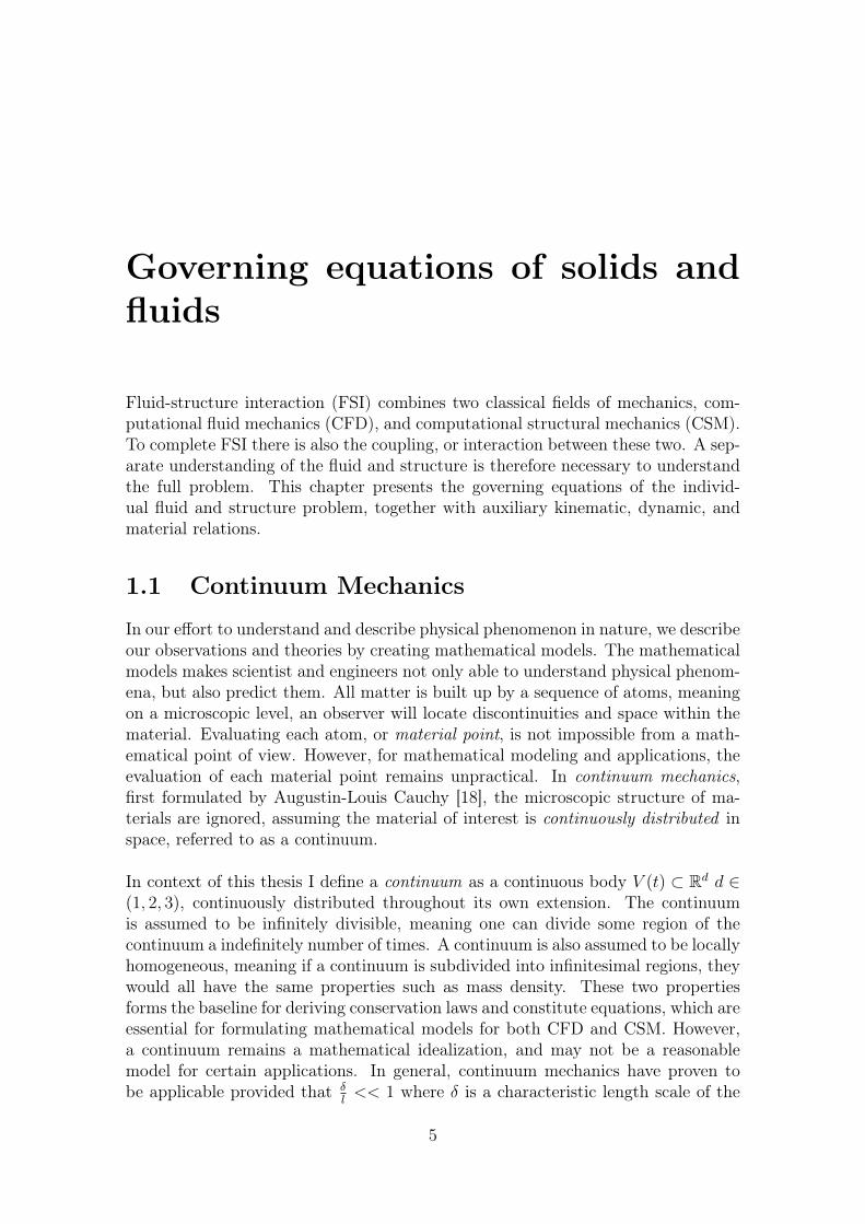
The Eulerian description falls naturally for describing fluid flow, due to local kine-matic properties are of higher interest rather than the shape of fluid domain. Usinga Lagrangian description for fluid flow would also be tedious, due to the large num-ber of material particles appearing for longer simulations of fluid flow. A comparisonof the two previous mentioned description is shown of In Figure 1.3.
Figure 1.3: Comparison of the Lagrangian and Eulerian description of motion.
8
Governing equations of solids and fluids
1.3 The Solid equations
The solid governing equations is given by,
Equation 1.3.1. Solid equations
ρs∂vs∂t
= ∇ · (JσsF−T ) + ρsfs in Ωs (1.3)
∂vs∂t
= us in Ωs (1.4)
defined in a Lagrangian coordinate system, with respect to an initial referenceconfiguration Ωs. The structure configuration is given by the displacement us, withthe relation ∂v
∂t= us to the solid velocity. The density of the structure is given
by ρs, and fs express any exterior body forces acting. Finally, F = I +∇us is thedeformation gradient, and J is the determinant of F 1.Material models express the dependency between strain tensors and stress. Thevalidity of material models is often limited by their ability to handle deformationand strain to some extent, before it breaks down or yields nonphysical observationsof the material. In this thesis, a linear relation between stress and strain is assumed,where the elasticity of the material is expressed by the Poisson ratio νs, Youngmodulus E, or Lamés coefficients λs and µs. Their relation is given by,
Ey =µs(λs + 2µs)
(λs + µs)νs =
λs2(λs + µs)
λs =νEy
(1 + νs)(1− 2νs)µs =
Ey2(1 + νs)
Hooke’s law is a linear relation applicable for small-scale deformations,
Definition 1.1. Let u be a differential deformation field in the reference configu-ration, I be the Identity matrix, and the gradient ∇ = ( ∂
∂x, ∂∂y, ∂∂z
). Hooke’s law isthen given by,
σs =1
JF(λs(Tr(ε)I + 2µε)F
Ss = λs(Tr(ε)I + 2µε
ε =1
2(∇u + (∇u)T )
However, as Hooke’s law is limited to a small-deformation, it is not valid for largedeformations encountered in this thesis. A valid model for larger deformations isthe hyper-elastic St. Vernant-Kirchhoff model(STVK), extending Hooke’s law intoa non-linear regime.
Definition 1.2. Let u be a differential deformation field in the reference con-figuration, I be the Identity matrix and the gradient ∇ = ( ∂
∂x, ∂∂y, ∂∂z
). The St.
1See Appendix A for further detail
9
3. The Solid equations
Vernant-Kirchhoff model is then given by the relation,
σs =1
JF(λs(Tr(E)I + 2µE)F−T
Ss = λs(Tr(E)I + 2µE
E =1
2(C− I) C = FF−T
where C is the right Cauchy-Green strain tensor and E is the Green Lagrangianstrain tensor.
Though STVK can handle large deformations, it is not valid for large strain [22].However since the strain considered in this thesis are small, it will remain ourprimary choice of strain-stress relation. In addition, initial condition and boundarycondition is supplemented for the problem to be well posed. The first type of ofboundary conditions are Dirichlet boundary conditions,
vs = vDs on ΓDs ⊂ ∂Ωs (1.5)ds = dDs on ΓDs ⊂ ∂Ωs (1.6)
(1.7)
The second type of boundary condition are Neumann boundary conditions
σs · n = g on ΓNs ⊂ ∂Ωs (1.8)
10

Governing equations of solids and fluids
1.4 The Fluid equations
The fluid is assumed to be express by the incompressible Navier-Stokes equations,
Equation 1.4.1. Navier-Stokes equation
ρ∂vf∂t
+ ρvf · ∇vf = ∇ · σ + ρff in Ωf (1.9)
∇ · vf = 0 in Ωf (1.10)
defined in an Eulerian description of motion. The fluid density as ρf and fluidviscosity νf are assumed to be constant in time, and fs represents any body force.The fluid is assumed Newtonian, where Cauchy stress sensor follows Hooke’s law
σ = −pfI + µf (∇vf + (∇vf )T
As for the solid equations, boundary conditions are supplemented considering Dirich-let boundary conditions,
vf = vDf on ΓDv ⊂ ∂Ωf (1.11)
pf = pDf on ΓDp ⊂ ∂Ωf (1.12)
The second type of boundary condition are Neumann boundary conditions
σf · n = g on ΓNf ⊂ ∂Ωf (1.13)
11

4. The Fluid equations
12
Fluid Structure Interaction
The multi-disciplinary nature of computational fluid-structure interaction, involvesaddressing issues regarding computational fluid dynamics and computational struc-ture dynamics. In general, CFD and CSM are individually well-studied in terms ofnumerical solution strategies. FSI adds another layer of complexity to the solutionprocess by the coupling of the fluid and solid equations, and the tracking of interfaceseparating the fluid and solid domains. The coupling pose two new conditions atthe interface absent from the original fluid and solid conditions, which is continuityof velocity and continuity of stress at the interface.
vf = vs (2.1)σf · n = σs · n (2.2)
The tracking of the interface is a issue, due to the different description of motionused in the fluid and solid problem. If the natural coordinate system are used for thefluid problem and solid problem, namely the Eulerian and Lagrangian description ofmotion, the domains doesn’t match and the interface. Tracking the interface is alsoessential for fulfilling the interface boundary conditions. As such only one of thedomains can be described in its natural coordinate system, while the other domainneeds to be defined in some transformed coordinate system. Fluid-structure interac-tion problems are formally divided into the monolithic and partitioned frameworks.In the monolithic framework, the fluid and solid equations together with interfaceconditions are solved simultaneously. The monolithic approach is strongly coupled,meaning the kinematic (1.1) and dynamic(1.2) interface conditions are met withhigh accuracy. However, the complexity of solving all the equations simultaneouslyand the strong coupling contributes to a stronger nonlinear behavior of the wholesystem [42]. The complexity also makes monolithic implementations ad hoc and lessmodular, and the nonlinearity makes solution time slow. In the partitioned frame-work one solves the equations of fluid and structure subsequently. Solving the fluidand solid problems individually is beneficial, in terms of the wide range of optimizedsolvers and solution strategies developed for each sub-problem. In fact, solving thefluid and solid separately was used in the initial efforts in FSI, due to existing solversfor one or both problems [10]. Therefore, computational efficiency and code reuse isone of the main reasons for choosing the partitioned approach. A major drawbackis the methods ability to enforce the kinematic (1.1) and dynamic(1.2) conditionsat each timestep. Therefore partitioned solution strategies are defined as weaklycoupled. However, by sub-iterations between each sub-problem at each timestep,
13

(1.1) and (1.2) can be enforced with high accuracy, at the cost of increased compu-tational time. Regardless of framework, FSI has to cope with a numerical artifactcalled the "added-mass effect" [5], [4], [8]. The term is not to be confused withadded mass found in fluid mechanics, were virtual mass is added to a system dueto an accelerating or de-accelerating body moving through a surrounding fluid [20].Instead, the term is used to describe the numerical instabilities occurring for weaklycoupled schemes, in conjunction with in compressible fluids and slender structures[8], or where the density of the incompressible fluid is close to the structure. For par-titioned solvers, sub-iterations are needed when the "added-mass effect" is strong,but for incompressible flow the restrictions can lead to unconditional instabilities[10]. The strong coupled monolithic schemes have proven overcome "added-masseffect" preserving energy balance, at the prize of a highly non-linear system to besolved at each time step [5]. Capturing the interface is matter of its own, regardlessof the the monolithic and partitioned frameworks. The scope of interface methodsare divided into interface-tracking and interface-capturing methods, visualized infigure 2.1.
Figure 2.1: Comparison of interface-tracking and interface-capturing for an elasticbeam undergoing deformation
In the Interface-tracking method, the mesh moves to accommodate for the move-ment of the structure as it deforms the spatial domain occupied by the fluid. Assuch, the mesh itself "tracks" the fluid-structure interface as the domain undergoesdeformation. Interface-capturing yields better control of mesh resolution near theinterface, which in turn yields better control of this critical area in terms of en-forcing the interface conditions. However, moving the mesh-nodes pose potentialproblems for mesh-entanglements, restricting the possible extent of deformations.In interface-capturing methods one distinguish the fluid and solid domains by somephase variable over a fixed mesh, not resolved by the mesh itself. This approachis in general not limited in terms of deformations, but suffers from reduced accu-racy at the interface. Among the multiple approaches within FSI, the arbitraryLagrangian-Eulerian method is chosen for this thesis.
14

Fluid Structure Interaction
2.1 Arbitrary Lagrangian Eulerian formulation
The arbitrary Lagrangian-Eulerian formulation is the most popular approach withinInterface-tracking [24, 9]. In this approach the structure is given in its naturalLagrangian coordinate system, while the fluid problem is formulated in an artificialcoordinate system similar to the Lagrangian coordinate system, by an artificial fluiddomain map from the undeformed reference configuration Tf (t) : Vf (t) → Vf (t).The methods consistency is to a large extent dependent on the regularity of theartificial fluid domain map. Loss of regularity can occur for certain domain motions,were the structure makes contact with domain boundaries or self-contact with otherstructure parts [23]. Since no natural displacement occur in the fluid domain,the transformation Tf (t) has no directly physical meaning [24, 3]. Therefore, theconstruction of the transformation Tf (t) is a purely numerical exercise.
2.1.1 ALE formulation of the fluid problem
The original fluid problem, defined by the incompressible Navier-Stokes equations(Equation 1.5.1). are defined in an Eulerian description of motion Vf (t). By chang-ing the computational domain to an undeformed reference configuration Vf (t) →Vf (t), the original problem no longer comply with the change of coordinate sys-tem. Therefore, the original Navier-Stokes equations needs to be transformed ontothe reference configuration Vf . Introducing the basic properties needed for map-ping between the sub-system Vf (t) and Vf (t), we will present the ALE time andspace derivative transformations found in [25], with help of a new arbitrary fixedreference system W. Let Tw : W→ V (t) be an invertible mapping, with the scalar
Figure 2.2: CFD-3, flow visualization of velocity time t = 9s
f(xW , t) = f(x, t) and vector w(xW , t) = w(x, t) counterparts. Further let the defor-mation gradient Fw and its determinant Jw, be defined in accordance wit definition1.1 and 1.2 in Chapter 1. Then the following relations between temporal and spatialderivatives apply, between the two domains W (t) and V (t),
15
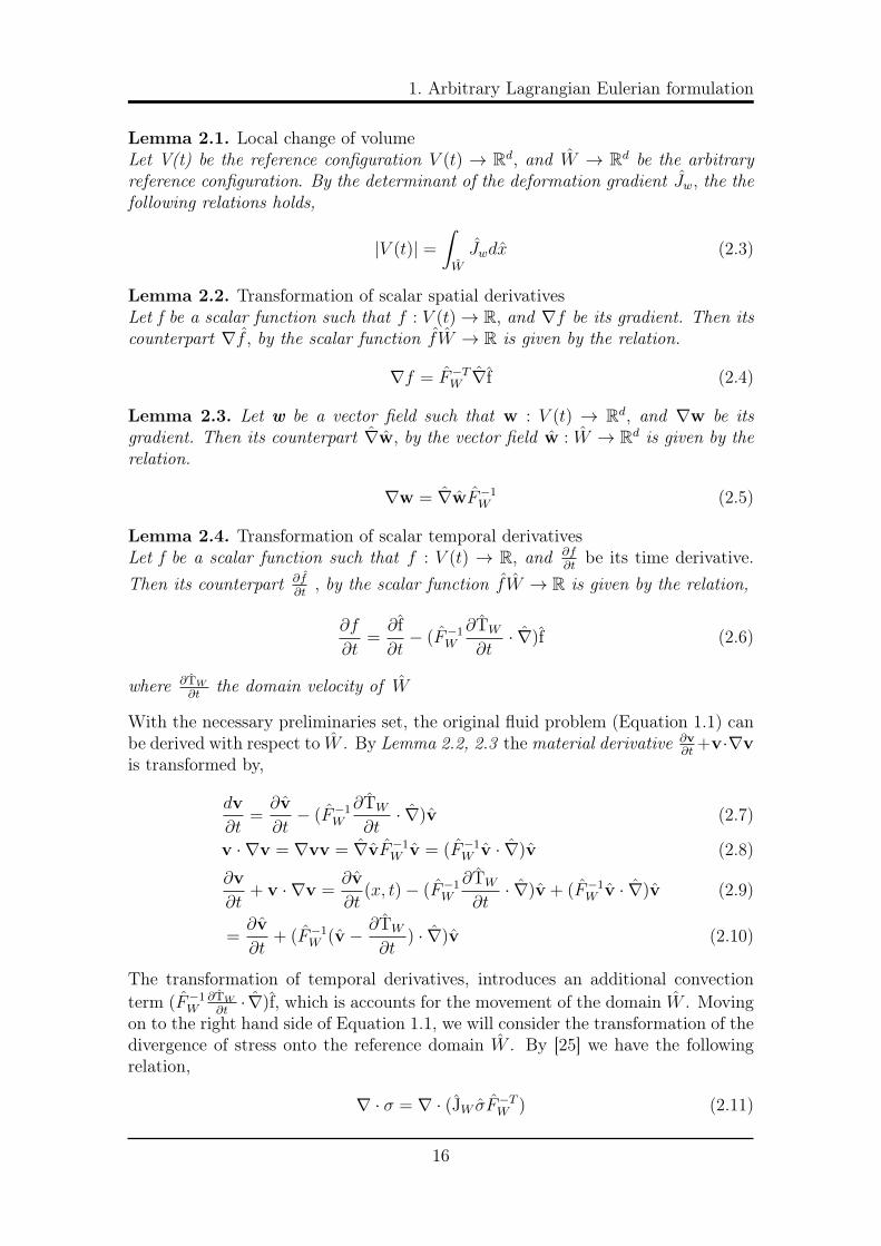
1. Arbitrary Lagrangian Eulerian formulation
Lemma 2.1. Local change of volumeLet V(t) be the reference configuration V (t) → Rd, and W → Rd be the arbitraryreference configuration. By the determinant of the deformation gradient Jw, the thefollowing relations holds,
|V (t)| =∫W
Jwdx (2.3)
Lemma 2.2. Transformation of scalar spatial derivativesLet f be a scalar function such that f : V (t)→ R, and ∇f be its gradient. Then itscounterpart ∇f , by the scalar function f W → R is given by the relation.
∇f = F−TW ∇f (2.4)
Lemma 2.3. Let w be a vector field such that w : V (t) → Rd, and ∇w be itsgradient. Then its counterpart ∇w, by the vector field w : W → Rd is given by therelation.
∇w = ∇wF−1W (2.5)
Lemma 2.4. Transformation of scalar temporal derivativesLet f be a scalar function such that f : V (t) → R, and ∂f
∂tbe its time derivative.
Then its counterpart ∂f∂t
, by the scalar function f W → R is given by the relation,
∂f
∂t=∂ f∂t− (F−1
W
∂TW
∂t· ∇)f (2.6)
where ∂TW
∂tthe domain velocity of W
With the necessary preliminaries set, the original fluid problem (Equation 1.1) canbe derived with respect to W . By Lemma 2.2, 2.3 thematerial derivative ∂v
∂t+v·∇v
is transformed by,
dv
∂t=∂v
∂t− (F−1
W
∂TW
∂t· ∇)v (2.7)
v · ∇v = ∇vv = ∇vF−1W v = (F−1
W v · ∇)v (2.8)
∂v
∂t+ v · ∇v =
∂v
∂t(x, t)− (F−1
W
∂TW
∂t· ∇)v + (F−1
W v · ∇)v (2.9)
=∂v
∂t+ (F−1
W (v − ∂TW
∂t) · ∇)v (2.10)
The transformation of temporal derivatives, introduces an additional convectionterm (F−1
W∂TW
∂t· ∇)f, which is accounts for the movement of the domain W . Moving
on to the right hand side of Equation 1.1, we will consider the transformation of thedivergence of stress onto the reference domain W . By [25] we have the followingrelation,
∇ · σ = ∇ · (JW σF−TW ) (2.11)
16

Fluid Structure Interaction
Were JW σF−TW is the first Piola Kirchhoff stress tensor, relating forces from a
Eulerian description of motion to the reference domain W . Assuming a Newtonianfluid, the Cauchy stress tensor takes the form σ = −pI + µf (∇v + (∇v)T . Sinceσ 6= σ in W , the spatial derivatives must be transformed, by using Lemma 2.2
σ = −pI + µf (∇v + (∇v)T
σ = −pI + µf (∇vF−1W + F−T
W ∇vT )
For the conservation of continuum we apply the Piola Transformation [25], suchthat
∇ · v = ∇ · (JF−1W v) (2.12)
As the central concepts for transforming the fluid problem on an arbitrary referencedomain are introduced, the notation W will no longer be used, instead replaced withthe fluid domain Ωf , inheriting all previous concepts presented in reference with W .Let Tf : Ωf → Ωf (t) be an invertible mapping, with the scalar f(xf , t) = f(x, t) andvf (xf , t) = vf (x, t) counterparts. Further let Ff be the deformation gradient andJw its determinant.
Equation 2.1.1. ALE fluid problemLet vf be the fluid velocity, ρf the fluid density, and νf the fluid viscosity.
Jf∂v
∂t+ Jf (F−1
f (v − ∂TW
∂t) · ∇)v = ∇ · (JW σF−T
W ) + ρf Jff in Ωf (2.13)
∇ · (JF−1W v) = 0 in Ωf (2.14)
where fs represents any exterior body force.
Due to the arbitrary nature of the reference system W , the physical velocity v andthe velocity of arbitrary domain ∂Ww
∂tdoesn’t necessary coincide, as it deals with
three different reference domains [25]. The Lagrangian particle tracking x ∈ Ωf ,the Eulerian tracking x ∈ Ωf , and the arbitrary tracking of the reference domainx ∈ W [25]. This concept can be further clarified by the introduction of materialand spatial points.
2.1.2 ALE formulation of the solid problemWith the introduced mapping identities we have the necessary tools to derive a fullfluid-structure interaction problem defined of a fixed domain. Since the structurealready is defined in its natural Lagrangian coordinate system, no further derivationsare needed for defining the total problem.
Equation 2.1.2. ALE solid problem
ρs∂vs∂t
= ∇ · FS + ρsfs in Ωs (2.15)
(2.16)
17
1. Arbitrary Lagrangian Eulerian formulation
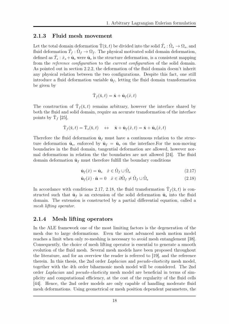
2.1.3 Fluid mesh movement
Let the total domain deformation T(x, t) be divided into the solid Ts : Ωs → Ωs, andfluid deformation Tf : Ωf → Ωf . The physical motivated solid domain deformation,defined as Ts : xs+ us were us is the structure deformation, is a consistent mappingfrom the reference configuration to the current configuration of the solid domain.As pointed out in section 2.2.2, the deformation of the fluid domain doesn’t inheritany physical relation between the two configurations. Despite this fact, one stillintroduce a fluid deformation variable uf , letting the fluid domain transformationbe given by
Tf (x, t) = x + uf (x, t)
The construction of Tf (x, t) remains arbitrary, however the interface shared byboth the fluid and solid domain, require an accurate transformation of the interfacepoints by Tf [25],
Tf (x, t) = Ts(x, t) ↔ x + uf (x, t) = x + us(x, t)
Therefore the fluid deformation uf must have a continuous relation to the struc-ture deformation us, enforced by uf = us on the interface.For the non-movingboundaries in the fluid domain, tangential deformation are allowed, however nor-mal deformations in relation the the boundaries are not allowed [24]. The fluiddomain deformation uf must therefore fulfill the boundary conditions
uf (x) = us x ∈ Ωf ∪ Ωs (2.17)
uf (x) · n = 0 x ∈ ∂Ωf 6= Ωf ∪ Ωs (2.18)
In accordance with conditions 2.17, 2.18, the fluid transformation Tf (x, t) is con-structed such that uf is an extension of the solid deformation us into the fluiddomain. The extension is constructed by a partial differential equation, called amesh lifting operator.
2.1.4 Mesh lifting operatorsIn the ALE framework one of the most limiting factors is the degeneration of themesh due to large deformations. Even the most advanced mesh motion modelreaches a limit when only re-meshing is necessary to avoid mesh entanglement [38].Consequently, the choice of mesh lifting operator is essential to generate a smoothevolution of the fluid mesh. Several mesh models have been proposed throughoutthe literature, and for an overview the reader is referred to [19], and the referencetherein. In this thesis, the 2nd order Laplacian and pseudo-elasticity mesh model,together with the 4th order biharmonic mesh model will be considered. The 2ndorder Laplacian and pseudo-elasticity mesh model are beneficial in terms of sim-plicity and computational efficiency, at the cost of the regularity of the fluid cells[44]. Hence, the 2nd order models are only capable of handling moderate fluidmesh deformations. Using geometrical or mesh position dependent parameters, the
18

Fluid Structure Interaction
models can be improved to handle a wider range of deformations, by increasing thestiffness of the cell close to the interface [14].
A limitation of the 2nd order mesh models is that by Dirichlet and Neumann bound-ary conditions, only mesh position or normal mesh spacing can be specified respect-fully, but not both [11]. This limitation is overcome by 4th order biharmonic meshmodel, since two boundary conditions can be specified at each boundary of the fluiddomain [11]. The 4th order biharmonic mesh model is superior for handling largefluid mesh deformations, as the model generates a better evolution of the fluid cells.A better regularity of the fluid cells also have the potential of less Newton iterationsneeded for convergence at each time-step [44], discussed in section 5.5. The modelis however much more computational expensive compared to the 2nd order meshmodels.
Mesh motion by a Laplacian lifting operator
Equation 2.1.3. The Laplace equation modelLet uf be the fluid domain deformation, us be the structure domain deformation,and let α be diffusion parameter raised to the power of some constant q. TheLaplacian mesh model is given by,
− ∇ · (αq∇u) = 0 Ωf
uf = us on Γ
uf = 0 on ∂Ωf/Γ
The choice of diffusion parameter is often problem specific, as selective treatmentof the fluid cells may vary from different mesh deformation problems. For smalldeformations, the diffusion-parameter α can be set to a small constant [45, 24].To accommodate for larger deformations, a diffusion-parameter dependent of meshparameters, such as fluid cell volume [2] or the Jacobian of the deformation gradient[35] have proven beneficial. In [16], the authors reviewed several options based onthe distance to the closest moving boundary. This approach will be used in thisthesis, using a diffusion-parameter inversely proportional to the magnitude of thedistance x, to the closest moving boundary,
α(x) =1
xqq = −1
19

1. Arbitrary Lagrangian Eulerian formulation
Mesh motion by a Linear elastic lifting operator
Equation 2.1.4. The linear elastic modelLet uf be the fluid domain deformation, us be the structure domain deformation,and let σ be the Cauchy stress tensor. The linear elastic mesh model is given by,
∇ · σ = 0 Ωf
uf = us on Γ
uf = 0 on ∂Ωf/Γ
σ = λTr(ε(uf ))I + 2µε(uf ) ε(u) =1
2(∇u+∇uT )
Where λ, µ are Lamés constants given by Young’s modulus E, and Poisson’s ratioν.
λ =νE
(1 + ν)(1− 2ν)µ =
E
2(1 + ν)
The fluid mesh deformation characteristics are in direct relation which the choice ofthe material specific parameters, Young’s modulus E and Poisson’s ratio µ. Young’smodulus E describes the stiffness of the material, while the Poisson’s ratio relateshow a materials shrinks in the transverse direction, while under extension in theaxial direction. However the choice of these parameters have proven not to beconsistent, and to be dependent of the given problem. In [43] the author proposeda negative Poisson ratio, which makes the model mimic an auxetic material, whichbecomes thinner in the perpendicular direction when submitted to compression.Another approach is to set ν ∈ [0, 0.5) and let E be inversely proportional to thecell volume [1], or inverse of the distance of an interior node to the nearest deformingboundary surface [19]. In this thesis, the latter is chosen merely for the purpose ofcode reuse from the Laplace mesh model, defined as,
ν = 0.1 E(x) =1
xqq = −1
20

Fluid Structure Interaction
Mesh motion by a Biharmonic lifting operator
Equation 2.1.5. The biharmonic mesh modelLet uf be the fluid domain deformation, us be the structure domain deformation.The biharmonic mesh model is given by,
∇4uf = 0 on Ωf
By introducing a second variable on the form w = −∇û, we get the following systemdefined by
w = −∇2u
− ∇w = 0
In combination with [43], two types of boundary conditions are proposed. Let ufbe decomposed by the components uf = (û(1)
f .û(2)f ). Then we have
Type 1 û(k)f =
∂û(k)f
∂n= 0 ∂Ωf/Γ for k = 1, 2
Type 2 û(1)f =
∂û(1)f
∂n= 0 and w(1)
f =∂w(1)
f
∂n= 0 on Ωin
f ∪ Ωoutf
û(2)f =
∂û(2)f
∂n= 0 and w(2)
f =∂w(2)
f
∂n= 0 on Ωwall
f
The first type of boundary condition the model can interpreted as the bending of athin plate, clamped along its boundaries. In addition to prescribed mesh position asthe Laplacian and linear-elastic model, an additional constraint to the mesh spacingis prescribed at the fluid domain boundary. The form of this problem has beenknown since 1811, and its derivation has been connected with names like Frenchscientists Lagrange, Sophie Germain, Navier and Poisson [17]. The second type ofboundary condition is advantageous when the reference domain Ωf is rectangular,constraining mesh motion only in the perpendicular direction of the fluid boundary.This constrain allows mesh movement in the tangential direction of the domainboundary, further reducing distortion of the fluid cells [43].
21

2. Discretization of the FSI problem
2.2 Discretization of the FSI problem
In this thesis, the finite element method will be used to discretize the coupled fluid-structure interaction problem. It is beyond of scope of this thesis, to thorough diveinto the analysis of the finite element method regarding fluid-structure interactionproblems. Only the basics of the method, which is necessary in order to define afoundation for problem solving will be introduced.
2.2.1 Finite Element method
Let the domain Ω(t) ⊂ Rd (d = 1, 2, 3) be a time dependent domain discretizeda by finite number of d-dimensional simplexes. Each simplex is denoted as a fi-nite element, and the union of these elements forms a mesh. Further, let the do-main be divided by two time dependent subdomains Ωf and Ωs, with the interfaceΓ = ∂Ωf ∩ ∂Ωs. The initial configuration Ω(t), t = 0 is defined as Ω, defined inthe same manner as the time-dependent domain. Ω is known as the reference con-figuration, and hat symbol will refer any property or variable to this domain. Theouter boundary is set by ∂Ω , with ∂ΩD and ∂ΩN as the Dirichlet and Neumannboundaries respectively.
The family of Lagrangian finite elements are chosen, with the function space nota-tion,
VΩ := H1(Ω) V 0Ω := H1
0 (Ω)
where Hn is the Hilbert space of degree n.Let Problem 2.1 denote the strong formulation. By the introduction of appropriatetrial and test spaces of our variables of interest, the weak formulation can be deducedby multiplying the strong form with a test function and taking integration by partsover the domain. The velocity variable is continuous through the solid and fluiddomain
VΩ,v := v ∈ H10 (Ω), vf = vs on Γi
VΩ,ψ := ψu ∈ H10 (Ω), vf = vs on Γi
For the deformation, and the artificial deformation in the fluid domain let
VΩ,v := u ∈ H10 (Ω), uf = us on Γi
VΩ,ψ := ψv ∈ H10 (Ω), ψv
f = ψvs on Γi
For simplification of notation the inner product is defined as∫Ω
v ψ dx = (v, ψ)Ω
22
Fluid Structure Interaction
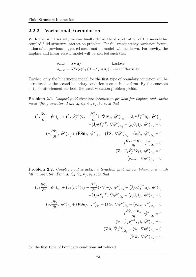
2.2.2 Variational Formulation
With the primaries set, we can finally define the discretization of the monolithiccoupled fluid-structure interaction problem. For full transparency, variation formu-lation of all previous suggested mesh motion models will be shown. For brevity, theLaplace and linear elastic model will be shorted such that
σmesh = α∇uf Laplaceσmesh = λTr(ε(uf ))I + 2µε(uf ) Linear Elasticity
Further, only the biharmonic model for the first type of boundary condition will beintroduced as the second boundary condition is on a similar form. By the conceptsof the finite element method, the weak variation problem yields.
Problem 2.1. Coupled fluid structure interaction problem for Laplace and elasticmesh lifting operator. Find us, uf , vs, vf , pf such that
(Jf∂vf∂t
, ψu)
Ωf+(Jf (F−1
f (vf −∂Tf
∂t) · ∇)vf , ψ
u)
Ωf+(Jf σF−T
f nf , ψu)
Γi
−(Jf σF−T
f , ∇ψu)
Ωf−(ρf Jf ff , ψu
)Ωf
= 0(ρs∂vs∂t
, ψu)
Ωs+(FSnf , ψ
u)
Γi−(FS, ∇ψu
)Ωs−(ρsfs, ψ
u)
Ωs= 0(∂vs − us
∂t, ψv
)Ωs
= 0(∇ · (Jf F−1
f vf ), ψp)
Ωf= 0(
σmesh, ∇ψu)
Ωf= 0
Problem 2.2. Coupled fluid structure interaction problem for biharmonic meshlifting operator. Find us, uf , vs, vf , pf such that
(Jf∂vf∂t
, ψu)
Ωf+(Jf (F−1
f (vf −∂Tf
∂t) · ∇)vf , ψ
u)
Ωf+(Jf σF−T
f nf , ψu)
Γi
−(Jf σF−T
f , ∇ψu)
Ωf−(ρf Jf ff , ψu
)Ωf
= 0(ρs∂vs∂t
, ψu)
Ωs+(FSnf , ψ
u)
Γi−(FS, ∇ψu
)Ωs−(ρsfs, ψ
u)
Ωs= 0(∂vs − us
∂t, ψv
)Ωs
= 0(∇ · (Jf F−1
f vf ), ψp)
Ωf= 0(
∇u, ∇ψη)
Ωf−(w, ∇ψu
)Ωf
= 0(∇w, ∇ψv
)Ωf
= 0
for the first type of boundary conditions introduced.
23
3. One-step θ scheme
Coupling conditions
Equation 2.2.1. Interface coupling conditions
vf = vs kinematic boundary condition(JW σF−T
W nf , ψu)
Ωf=(FSns, ψ
u)
Ωsdynamic boundary condition
By a continuous velocity field on the whole domain, the kinematic condition isstrongly enforced on the interface Γi. The dynamic boundary condition is weaklyimposed by omitting the boundary integral from the variational formulation, be-coming an implicit condition for the system [42].
2.3 One-step θ scheme
For both the fluid problem and the structure problem, we will base our implemen-tation on a θ-scheme. A θ-scheme is favorable, making implementation of classicaltime-stepping schemes simple. For the structure problem, θ-scheme takes the form
ρs∂vs∂t− θ∇ · FS− (1− θ)∇ · FS− θρsfs − (1− θ)ρsfs = 0
∂vs∂t− θus − (1− θ)us = 0
For θ ∈ [0, 1] classical time-stepping schemes are obtained such as the first-orderforward-Euler scheme θ = 0, backward-Euler scheme θ = 1, and the second-orderCrank-Nicholson scheme θ = 1
2. Studying the fluid problem, it is initially simpler
to consider the Navier-Stokes equation in an Eulerian formulation rather the ALE-formulation Following [33], a general time stepping algorithm for the coupled Navier-Stokes equation can be written as
1
∆(un+1 − un) +B(u∗)un+α − ν∇2un+α = −∇p+ un+α
∇ · un+α = 0
Here un+α is an "intermediate" velocity defined by,
un+α = αun+1 + (1− α)un α ∈ [0, 1]
while u∗ is on the form
u∗ = un+ϑ =
ϑun+1 + (1− ϑ)un ϑ ≥ 0
ϑun−1 + (1− ϑ)un ϑ ≤ 0
At first glance, defining an additional parameter ϑ for the fluid problem seemsunnecessary. A general mid-point rule by α = ϑ = 1
2, a second order scheme
in time would easily be achieved. However, in [33] an additional second order
24
Fluid Structure Interaction
scheme is obtained by choosing e α = 12, ϑ = −1, where u∗ is approximated with
an Adam-Bashforth linear method. Making the initial fluid problem linear whilemaintaining second order convergence is an important result, which have not yetbeen investigated thorough in literature of fluid-structure interaction. However, inthe monolithic ALE method presented in this thesis, the fluid problem will stillremain non-linear due to the ALE-mapping of the convective term, but makingthe overall problem "more linear" in contrary with a second order Crank-Nicolsonscheme. The idea was initially pursued in this thesis but left aside, as discretizationof the fluid convective term was not intuitive.By letting α = ϑ α, ϑ ∈ [0, 1] for the fluid problem, and generalizing the conceptsin an ALE context, we derive the one-step θ scheme found in [43].
Problem 2.3. The one-step θ scheme Find us, uf , vs, vf , pf such that
(Jn,θ ∂v
∂t, ψu
)Ωf
+
θ(JF−1
W (v · ∇)v, ψu)
Ωf+ (1− θ)
(JF−1
W (v · ∇)v, ψu)
Ωf
−(J∂TW
∂t· ∇)v, ψu
)Ωf− θ(JW σF−T
W , ∇ψu)
Ωf−−(1− θ)
(JW σF−T
W , ∇ψu)
Ωf
−θ(ρf Jff , ψu
)Ωf− (1− θ)
(ρf Jff , ψu
)Ωf
= 0(ρs∂vs∂t
, ψu)
Ωs+−θ
(FS, ∇ψu
)Ωs
+−(1− θ)(FS, ∇ψu
)Ωs
−θ(ρsfs, ψ
u)
Ωs− (1− θ)
(ρsfs, ψ
u)
Ωs= 0(∂vs
∂t− θus − (1− θ)us, ψv
)Ωs
= 0(∇ · (JF−1
W v), ψp)
Ωf= 0(
σmesh, ∇ψu)
Ωf= 0
25
3. One-step θ scheme
26

Verification and Validation
Computer simulations are in many engineering applications a cost-efficient methodof conducting design and optimize performance. However, blindly trusting resultsgenerated from a computer simulations can prove to be naive. It doesn’t take alot of coding experience before one realizes many things that can brake down andproduce unwanted or unexpected results. Therefore, credibility of computationalresults are essential, meaning the simulation is worthy of belief or confidence [21].For rigid evaluation of numerical models we use verification and validation (V&V )[34]. For a in-depth discussion of all aspects surrounding V&V the reader is referredto [21]. In this thesis, we follow the definitions provided by the American Society ofMechanical Engineers guide for Verification and Validation in Computational SolidMechanics [31]:
Definition 3.1. Verification: The process of determining that a computationalmodel accurately represents the underlying mathematical model and its solution.
Definition 3.2. Validation: The process of determining the degree to which amodel is an accurate representation of the real world from the perspective of theintended uses of the model.
Simplified, verification considers if one solves the equations right, while validationis checking if one solves the right equations for the given problem [28]. Verificationand validation is per definition an ongoing processes, with no clear boundary ofcompleteness unless additional requirements are specified [28]. The goal of thischapter is to verify the implementations using the method of manufactured solution(MMS), and addressing validation in a subsequent chapter.
3.1 Verification of Code
Within scientific computing a mathematical model is often the baseline for simula-tions of a particular problem of interest. For scientists exploring physical phenom-ena, the mathematical model is often on the form of systems of partial differentialequations (PDEs). Through verification of code, the ultimate goal is to ensure thatthe computer program correctly represents the mathematical model. To accumu-late sufficient evidence that a mathematical model is solved correctly by a computercode, it must excel within predefined criteria. If the acceptance criterion is not sat-isfied, a coding mistake is suspected. Should the code pass the preset criteria, the
27

1. Verification of Code
code is considered verified. Of the different classes of test found in [28], order-of-accuracy is regarded as the most rigorous [30, 28, 36]. The method tests if thediscretization error E is reduced in accordance with the formal order of accuracyexpected from the numerical scheme. The formal order of accuracy is defined to bethe theoretical rate at which the truncation error of a numerical scheme is expectedto reduce. The observed order of accuracy is the actual rate produced by the nu-merical solution. For order of convergence tests, the code is assumed to be verifiedif we recover the theoretical convergence from the discretization error. Monitoringthe discretization error E by spatial and temporal refinements, one assumes theerror E can be expressed as,
E = C∆tp +D∆xl
where C and D are constants, ∆t and ∆x represents the spatial and temporalresolution, while p and l is the observed order of accuracy of the numerical scheme.In order to calculate the convergence in space l, the spatial discretization error mustbe negligible compared to the temporal discretization error C∆tp. The total errorcan then by expressed as E = D∆xl, and we calculate the convergence rate forsubsequent spatial mesh refinement by,
E2
E1
= (∆x2
∆x1
)l (3.1)
l =log(E2
E1)
log(∆x2∆x1
)(3.2)
where E2 is computed on a finer mesh compared to E1 on a courser mesh. Forspatial convergence tests, the same procedure applies by choosing a high resolutiontemporal discretization, and calculating the error E1,E2 by subsequent smaller timesteps. In order to calculate order of convergence we need to find an exact solution ofthe problem. Creating an exact solution is often non-trivial. However, the methodof manufactured solution provides an efficient way of generating exact solutions.
3.1.1 Method of manufactured solutionSolutions to Navier-Stokes is limited and simplifications of the original problemare often necessary to produce analytical solutions. The method of manufacturedsolutions provides a simple yet robust way of creating analytic solutions. Let partialdifferential equation of interest be on the form
L(u) = f
Here L is a differential operator, u is variable the of interest, and f is somesourceterm. Normally, one would find u by solving the system. However, in MMSone first chooses a suitable u, and insert it into equation 3.3, which produces asource term f. Thus, when solving the system with the obtained f, we know theexact solution. Another appealing feature of MMS is that the chosen u does nothave to take into account the physical properties of the problem [27].
28
Verification and Validation
If the MMS is not chosen properly, the test will not work. Therefore, some guidelinesfor rigorous verification have been proposed in [36, 30, 27]:
• The manufactured solution should be composed of smooth analytic functionssuch as exponential, trigonometric, or polynomials.
• The manufactured solution should should have sufficient number of deriva-tives, exercising all terms and derivatives of the PDEs.
To properly verify the robustness of the method of manufactured solution, a reportregarding code verification through the method manufactured solution for the time-dependent Navier-Stokes equation was published by Salari and Knupp [30]. Toprove its robustness, the authors deliberate implemented code errors in a verifiedNavier-Stokes solver. In total 21 blind test-cases where implemented, where differentapproaches of verification frameworks were tested. Of these, 10 coding mistakes thatreduced the observed order-of-accuracy was implemented. The MMS captured allcoding mistakes, except one. This mistake would, accordingly to Roach [30], beencaptured if his guidelines for exact initial conditions had been followed.In general, computing the source term f can be quite challenging and error prone.Therefore, symbolic computation of the sourceterm is advantageous to overcomemistakes which can easily occur when calculating by hand. For construction of thesourceterm f, the Unified Form Language (UFL) provided in FEniCS Project willbe used.
Comment on verification of the fluid-structure interactionsolver by MMSAlthough the MMS does not need to take any physics into account, there are oftenmathematical constrictions from the problem it self. From section Section 2.2 wehave:Let vs, vf be the structure and fluid velocity, and let σs, σf be the Cauchy stresstensor for the structure and fluid respectively. Let ni be the normal vector pointingout of the domain i. We then have the following interface boundary conditions.:
1. Kinematic boundary condition vs = vf , enforced strongly by a continuousvelocity field in the fluid and solid domain.
2. Dynamic boundary condition σs · ns = σf · nf , enforced weakly by omittingthe boundary integrals from the weak formulation in problem.
The choice of a MMS is therefore not trivial, as it must fulfill condition 1 and 2,in addition to the divergence-free condition in the fluid, and avoiding cancellationof the ALE-convective term ∂Tf
∂t. The construction of a MMS for a monolithic FSI
problem is therefore out of the scope of this thesis. The struggle is reflected ofthe absence of research, regarding MMS for coupled FSI solvers in the literature.The problem is often circumvented, such as [32], where the verification process isconducted by the fluid and structure solver separately. Instead, the accuracy of thecoupling is evaluated by the code validation. The approach clearly ease the process,
29
1. Verification of Code
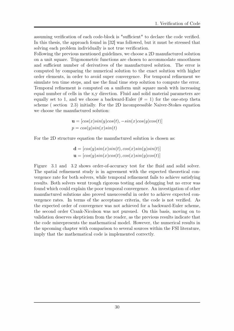
assuming verification of each code-block is "sufficient" to declare the code verified.In this thesis, the approach found in [32] was followed, but it must be stressed thatsolving each problem individually is not true verification.Following the previous mentioned guidelines, we choose a 2D manufactured solutionon a unit square. Trigonometric functions are chosen to accommodate smoothnessand sufficient number of derivatives of the manufactured solution. The error iscomputed by comparing the numerical solution to the exact solution with higherorder elements, in order to avoid super convergence. For temporal refinement wesimulate ten time steps, and use the final time step solution to compute the error.Temporal refinement is computed on a uniform unit square mesh with increasingequal number of cells in the x,y direction. Fluid and solid material parameters areequally set to 1, and we choose a backward-Euler (θ = 1) for the one-step thetascheme ( section 2.3) initially. For the 2D incompressible Naiver-Stokes equationwe choose the manufactured solution:
u = [cos(x)sin(y)cos(t),−sin(x)cos(y)cos(t)]
p = cos(y)sin(x)sin(t)
For the 2D structure equation the manufactured solution is chosen as:
d = [cos(y)sin(x)sin(t), cos(x)sin(y)sin(t)]
u = [cos(y)sin(x)cos(t), cos(x)sin(y)cos(t)]
Figure 3.1 and 3.2 shows order-of-accuracy test for the fluid and solid solver.The spatial refinement study is in agreement with the expected theoretical con-vergence rate for both solvers, while temporal refinement fails to achieve satisfyingresults. Both solvers went trough rigorous testing and debugging but no error wasfound which could explain the poor temporal convergence. An investigation of othermanufactured solutions also proved unsuccessful in order to achieve expected con-vergence rates. In terms of the acceptance criteria, the code is not verified. Asthe expected order of convergence was not achieved for a backward-Euler scheme,the second order Crank-Nicolson was not pursued. On this basis, moving on tovalidation deserves skepticism from the reader, as the previous results indicate thatthe code misrepresents the mathematical model. However, the numerical results inthe upcoming chapter with comparison to several sources within the FSI literature,imply that the mathematical code is implemented correctly.
30
Verification and Validation
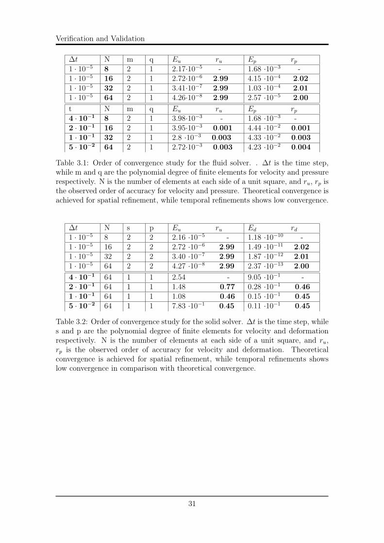
∆t N m q Eu ru Ep rp1 · 10−5 8 2 1 2.17·10−5 - 1.68 ·10−3 -1 · 10−5 16 2 1 2.72·10−6 2.99 4.15 ·10−4 2.021 · 10−5 32 2 1 3.41·10−7 2.99 1.03 ·10−4 2.011 · 10−5 64 2 1 4.26·10−8 2.99 2.57 ·10−5 2.00
t N m q Eu ru Ep rp4 · 10−1 8 2 1 3.98·10−3 - 1.68 ·10−3 -2 · 10−1 16 2 1 3.95·10−3 0.001 4.44 ·10−2 0.0011 · 10−1 32 2 1 2.8 ·10−3 0.003 4.33 ·10−2 0.0035 · 10−2 64 2 1 2.72·10−3 0.003 4.23 ·10−2 0.004
Table 3.1: Order of convergence study for the fluid solver. . ∆t is the time step,while m and q are the polynomial degree of finite elements for velocity and pressurerespectively. N is the number of elements at each side of a unit square, and ru, rp isthe observed order of accuracy for velocity and pressure. Theoretical convergence isachieved for spatial refinement, while temporal refinements shows low convergence.
∆t N s p Eu ru Ed rd1 · 10−5 8 2 2 2.16 ·10−5 - 1.18 ·10−10 -1 · 10−5 16 2 2 2.72 ·10−6 2.99 1.49 ·10−11 2.021 · 10−5 32 2 2 3.40 ·10−7 2.99 1.87 ·10−12 2.011 · 10−5 64 2 2 4.27 ·10−8 2.99 2.37 ·10−13 2.00
4 · 10−1 64 1 1 2.54 - 9.05 ·10−1 -2 · 10−1 64 1 1 1.48 0.77 0.28 ·10−1 0.461 · 10−1 64 1 1 1.08 0.46 0.15 ·10−1 0.455 · 10−2 64 1 1 7.83 ·10−1 0.45 0.11 ·10−1 0.45
Table 3.2: Order of convergence study for the solid solver. ∆t is the time step, whiles and p are the polynomial degree of finite elements for velocity and deformationrespectively. N is the number of elements at each side of a unit square, and ru,rp is the observed order of accuracy for velocity and deformation. Theoreticalconvergence is achieved for spatial refinement, while temporal refinements showslow convergence in comparison with theoretical convergence.
31

2. Validation
3.2 Validation
Through verification, one can assure that a scientific code evaluate mathematicalmodel correctly. However, accuracy is unnecessary if the model fails to serve as anappropriate representation of the physical problem. By definition 3.2, Validationis the act of demonstrating that a mathematical model is applicable for its intendeduse with a certain degree of accuracy. That is, a mathematical model is validated ifit meets some predefined criteria within a specific context. Validation is thereforenot intended to portray the model as an absolute truth, nor the best model available[29].In scientific computing, validation is traditionally conducted by comparing numer-ical results against existing experimental data, considered to be ground truth. Thedesign of validation experiments vary by the motivation of their creators. Vali-dated experiments for computational science can be divided into three groups [34]:(1) To improve fundamental understanding of a physical process, (2) Discovery orenhancement of mathematical models of well known physical processes, (3) To con-clude the reliability and performance of systems. Comparing numerical results andexperimental data, makes validation assess a wide range of issues [34]. Is the exper-iment relevant, and conducted correctly in accordance with prescribed parameters?What about the measurement uncertainty of reference experimental data? Theseissues must be addressed in order to raise sufficient confidence that the mathemat-ical model is credible for its intended use.
3.2.1 Validation benchmarkThe numerical benchmark presented in [13] has been chosen for validation of theOne-step θ scheme from chapter 3. The benchmark has been widely accepted as arigid validation benchmark throughout the literature [41, 42, 10]. This is mainlydue to the diversity of tests included, challenging all the main components of a fluid-structure interaction scheme. The benchmark is based on the a CFD benchmark[39], where a cylinder is placed off-center in a 2D channel. In [13], an additionalelastic flag is placed behind the cylinder, see Figure 4.1 The benchmark is dividedinto three problems, each further divided into three different sub-problems withincreasing complexity. In the first problem, the fluid solver is tested for differentinlet flow profiles. The second problem considers the structure solver, evaluatingthe bending of the elastic flag. And the final problem concerns validation of afull fluid-structure interaction problem with the fluid and the elastic flag. Severalquantities for comparison are presented in [13] for validation purposes:
• The position (x,y) of point A(t) as the elastic flag undergoes deformation.
• Drag and lift forces exerted on of the whole interior geometry in contact withthe fluid, consisting of the rigid circle and the elastic beam.
(FD, FL) =
∫Γ
σ · ndS
32

Verification and Validation
Figure 3.1: Computational domain of the validation benchmark.
All problems pose both steady state and periodic solutions. For the steady statesolutions, the quantity of interest will be calculated based on a transient simulation,that has converged towards a steady state solution. For the periodic solutions, theamplitude and mean values for the time dependent quantity are calculated from thelast period.
mean =1
2max + min (3.3)
amplitude =1
2max - min (3.4)
In [13], all steady state solutions seems to be calculated by solving a steady stateequation since time-step are only reported for the periodic solutions. In this the-sis, all problems in [13] are calculated using time integration. The main reason forsolving the problem transiently rather than steady state, is that numerical errorsassociated with initial transients are negligible with a sufficiently low time step size,without laborious changes to the numerical implementation. In the following sec-tion, an overview of each problem together with numerical results will be presented.A discussion of the results are given at the end of each simulation problem. Foreach table, the relative error of the finest spatial and temporal refinement comparedto the reference solution is reported in [13].
33
2. Validation
3.2.2 Validation of fluid solverThe validation test of the fluid solver addresses transient flow for a low Reynolds-number regime. We can take to different approaches to this problem [13]. The firstone considers the setup as a fluid-structure interaction problem, setting the materialproperties to mimic a stiff rod. In the second approach, the flag is excluded fromthe computational domain. Thus, any influence from the structure is eliminated.In this thesis, I choose to use second approach.Let vf , pf be the fluid velocity and pressure, and let σf be the Cauchy stress tensor,and ff denote any sourceterm, Find vf , pf such that :
(∂vf∂t
, ψu)
Ωf+((vf · ∇)vf , ψ
u)
Ωf−(σ, ∇ψu
)Ωf−(ρf ff , ψ
u)
Ωf= 0(
∇ · vf ), ψp)
Ωf= 0
The validation of the fluid solver is divided into three sub-problems; CFD-1, CFD-2,
parameter CFD-1 CFD-2 CFD-3ρf [103 kg
m3 ] 1 1 1νf [10−3m2
s] 1 1 1
U 0.2 1 2Re 20 100 200
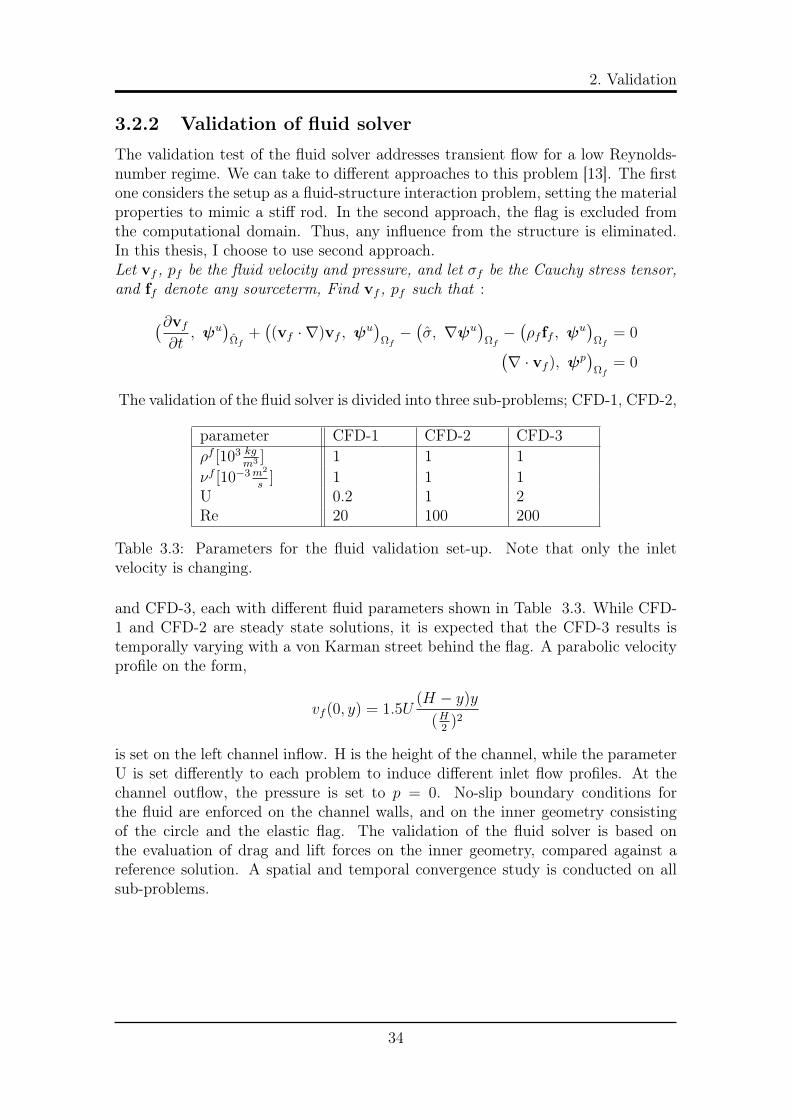
Table 3.3: Parameters for the fluid validation set-up. Note that only the inletvelocity is changing.
and CFD-3, each with different fluid parameters shown in Table 3.3. While CFD-1 and CFD-2 are steady state solutions, it is expected that the CFD-3 results istemporally varying with a von Karman street behind the flag. A parabolic velocityprofile on the form,
vf (0, y) = 1.5U(H − y)y
(H2
)2
is set on the left channel inflow. H is the height of the channel, while the parameterU is set differently to each problem to induce different inlet flow profiles. At thechannel outflow, the pressure is set to p = 0. No-slip boundary conditions forthe fluid are enforced on the channel walls, and on the inner geometry consistingof the circle and the elastic flag. The validation of the fluid solver is based onthe evaluation of drag and lift forces on the inner geometry, compared against areference solution. A spatial and temporal convergence study is conducted on allsub-problems.
34

Verification and Validation
Results
Table 3.4, 3.5, and 3.6 below shows the numerical solution of each sub-problem,CFD-1, CFD-2, and CFD-3. Each sub-problem is evaluated on four different meshwith increasing resolution. For the numerical solution of CFD-3 in Table 4.4, ad-ditional temporal and spatial refinement studies are conducted. Figure 4.1 showsthe evaluation of lift and drag for the finest spatial and temporal resolution, whileFigure 4.3 shows a visual representation of the fluid flow through the channel. Thenumerical solutions of CFD-1 in Figure 4.2 shows convergence against the referencesolution. Choosing P2-P1 elements together with a fully implicit scheme θ = 1,a relative error of 0.006% for lift, and 0% for drag is attained. For the numeri-cal solution of CFD-2 presented in Figure 4.3, the same observations apply. Thesecond order Crank-Nicolson scheme θ = 0.5 was investigated for CFD-1 and CFD-2, however only improving the results of order 10−6 for both lift and drag. Forthe periodic problem CFD-3, the choice of P2-P1 elements with a fully implicittime-stepping scheme proved insufficient for capturing the expected periodic solu-tion. Using Crank-Nicolson time-stepping scheme θ = 0.5, the periodic solutionwas attained.
∆t = 0.1 θ = 1.0nel ndof Drag Lift1438 6881 13.60 1.0892899 13648 14.05 1.1267501 34657 14.17 1.10919365 88520 14.20 1.119
Reference 14.29 1.119Error 0.006 % 0.00 %
Table 3.4: CFD-1 results, lift and drag evaluated at the inner geometry surface forincreasing spatial refinement. The error is computed as the relative error from thehighest mesh resolution against the reference solution.
∆t = 0.01 θ = 1.0nel ndof Drag Lift1438 6881 (P2-P1) 126.0 8.622899 13648 (P2-P1) 131.8 10.897501 34657 (P2-P1) 135.1 10.4819365 88520(P2-P1) 135.7 10.55
Reference 136.7 10.53Error 0.007 % 0.001 %
Table 3.5: CFD-2 results, lift and drag evaluated at the inner geometry surface forincreasing spatial refinement. The error is computed as the relative error from thehighest mesh resolution against the reference solution.
35
2. Validation
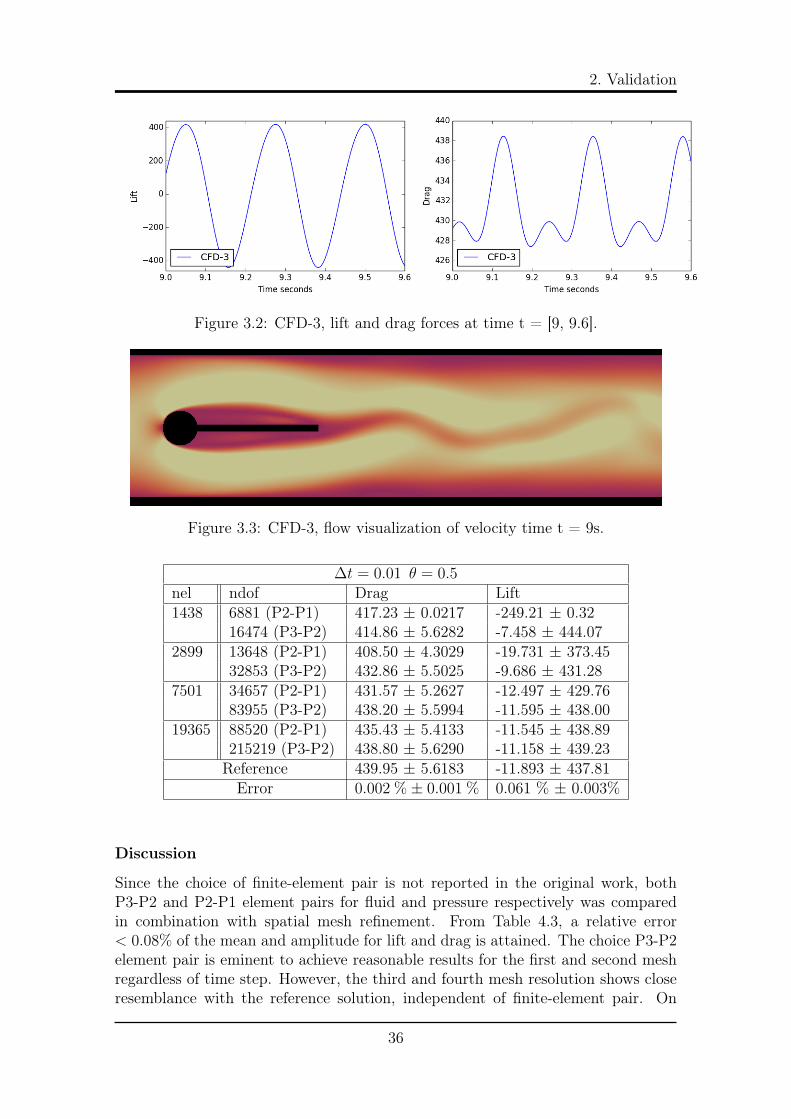
Figure 3.2: CFD-3, lift and drag forces at time t = [9, 9.6].
Figure 3.3: CFD-3, flow visualization of velocity time t = 9s.
∆t = 0.01 θ = 0.5nel ndof Drag Lift1438 6881 (P2-P1) 417.23 ± 0.0217 -249.21 ± 0.32
16474 (P3-P2) 414.86 ± 5.6282 -7.458 ± 444.072899 13648 (P2-P1) 408.50 ± 4.3029 -19.731 ± 373.45
32853 (P3-P2) 432.86 ± 5.5025 -9.686 ± 431.287501 34657 (P2-P1) 431.57 ± 5.2627 -12.497 ± 429.76
83955 (P3-P2) 438.20 ± 5.5994 -11.595 ± 438.0019365 88520 (P2-P1) 435.43 ± 5.4133 -11.545 ± 438.89
215219 (P3-P2) 438.80 ± 5.6290 -11.158 ± 439.23Reference 439.95 ± 5.6183 -11.893 ± 437.81Error 0.002 % ± 0.001 % 0.061 % ± 0.003%
Discussion
Since the choice of finite-element pair is not reported in the original work, bothP3-P2 and P2-P1 element pairs for fluid and pressure respectively was comparedin combination with spatial mesh refinement. From Table 4.3, a relative error< 0.08% of the mean and amplitude for lift and drag is attained. The choice P3-P2element pair is eminent to achieve reasonable results for the first and second meshregardless of time step. However, the third and fourth mesh resolution shows closeresemblance with the reference solution, independent of finite-element pair. On
36
Verification and Validation
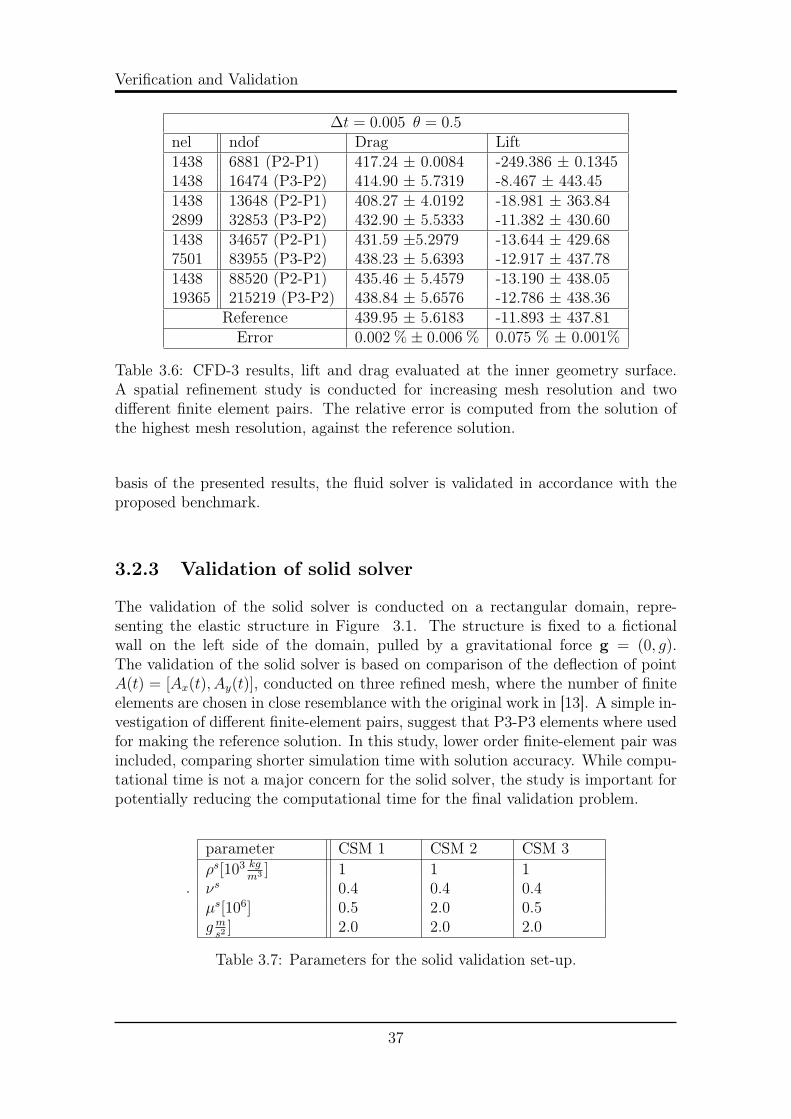
∆t = 0.005 θ = 0.5nel ndof Drag Lift1438 6881 (P2-P1) 417.24 ± 0.0084 -249.386 ± 0.13451438 16474 (P3-P2) 414.90 ± 5.7319 -8.467 ± 443.451438 13648 (P2-P1) 408.27 ± 4.0192 -18.981 ± 363.842899 32853 (P3-P2) 432.90 ± 5.5333 -11.382 ± 430.601438 34657 (P2-P1) 431.59 ±5.2979 -13.644 ± 429.687501 83955 (P3-P2) 438.23 ± 5.6393 -12.917 ± 437.781438 88520 (P2-P1) 435.46 ± 5.4579 -13.190 ± 438.0519365 215219 (P3-P2) 438.84 ± 5.6576 -12.786 ± 438.36
Reference 439.95 ± 5.6183 -11.893 ± 437.81Error 0.002 % ± 0.006 % 0.075 % ± 0.001%
Table 3.6: CFD-3 results, lift and drag evaluated at the inner geometry surface.A spatial refinement study is conducted for increasing mesh resolution and twodifferent finite element pairs. The relative error is computed from the solution ofthe highest mesh resolution, against the reference solution.
basis of the presented results, the fluid solver is validated in accordance with theproposed benchmark.
3.2.3 Validation of solid solver
The validation of the solid solver is conducted on a rectangular domain, repre-senting the elastic structure in Figure 3.1. The structure is fixed to a fictionalwall on the left side of the domain, pulled by a gravitational force g = (0, g).The validation of the solid solver is based on comparison of the deflection of pointA(t) = [Ax(t), Ay(t)], conducted on three refined mesh, where the number of finiteelements are chosen in close resemblance with the original work in [13]. A simple in-vestigation of different finite-element pairs, suggest that P3-P3 elements where usedfor making the reference solution. In this study, lower order finite-element pair wasincluded, comparing shorter simulation time with solution accuracy. While compu-tational time is not a major concern for the solid solver, the study is important forpotentially reducing the computational time for the final validation problem.
.
parameter CSM 1 CSM 2 CSM 3ρs[103 kg
m3 ] 1 1 1νs 0.4 0.4 0.4µs[106] 0.5 2.0 0.5gms2
] 2.0 2.0 2.0
Table 3.7: Parameters for the solid validation set-up.
37

2. Validation
Results
The numerical results for CSM-1, CSM-2, and CSM-3 are presented in table 3.8,3.9, 3.10, and 3.11. For the steady state sub-problems CSM-1 and CSM-2, a spatialconvergence study is conducted through mesh refinement with three different finite-element pairs. For the periodic CSM-3 problem, an additional temporal study wasconducted for two different time steps. In Figure 3.4, a visualization of CSM-3 isprovided for three different time steps. Finally, Figure 3.5 shows the displacementvector components, comparing all finite-element pairs for the finest mesh resolution.For CSM-1, the relative error of deformation found in Table 4.6, is 1.41% and 0.8%for the x and y coordinate respectively. In Table 4.7, a relative error of 1.49%and 0.88% for the x,y components can be found for CSM-2, proving both steadystate problems coincide with the reference solution. In Table 4.8, the numericalsolutions CSM-3 for time steps ∆t = 0.01 and ∆t = 0.005, are in close resemblancewith the reference solution. The study of lower-order elements proved successful forall problems, justifying accurate results can be achieved using P2-P2 elements fordeformation and velocity, even for coarse mesh resolution.
∆t = 0.1 θ = 1.0nel ndof ux of A [x 10−3] uy of A [x 10−3]319 832 P1-P1 -5.278 -56.6
2936 P2-P2 -7.056 -65.46316 P3-P3 -7.064 -65.5
1365 3140 P1-P1 -6.385 -62.211736 P2-P2 -7.075 -65.525792 P3-P3 -7.083 -65.5
5143 11084 P1-P1 -6.905 -64.742736 P2-P2 -7.083 -65.494960 P3-P3 -7.085 -65.5
Reference -7.187 -66.1Error 1.41 % 0.8 %
Table 3.8: CSM-1, deformation components of A(t) for ∆t = 0.1 and increasingspatial refinement. The error is computed as the relative error from the highestmesh resolution against the reference solution.
38

Verification and Validation
∆t = 0.05 θ = 1.0nel ndof ux of A [x 10−3] uy of A [x 10−3]319 832 P1-P1 -0.3401 -14.43
2936 P2-P2 -0.460 -16.786316 P3-P3 -0.461 -16.79
1365 3140 P1-P1 -0.414 -15.9311736 P2-P2 -0.461 -16.8125792 P3-P3 -0.461 -16.82
5143 11084 P1-P1 -0.449 -16.6042736 P2-P2 -0.461 -16.8294960 P3-P3 -0.462 -16.82
Reference -0.469 -16.97Error 1.49% 0.88 %
Table 3.9: CSM-2, deformation components of A(t) for ∆t = 0.05 and increasingspatial refinement. The error is computed as the relative error from the highestmesh resolution against the reference solution.
∆t = 0.01 θ = 0.5nel ndof ux of A [x 10−3] uy of A [x 10−3]319 832 P1-P1 -10.835 ± 10.836 -55.197 ± 56.845
2936 P2-P2 -14.390 ± 14.392 -63.303 ± 65.1496316 P3-P3 -14.432 ± 14.435 -63.397 ± 65.263
1365 3140 P1-P1 -13.053 ± 13.054 -60.367 ± 62.24111736 P2-P2 -14.428 ± 14.432 -63.388 ± 65.25625792 P3-P3 -14.444 ± 14.446 -63.432 ± 65.287
5143 11084 P1-P1 -14.082 ± 14.084 -62.656 ± 64.49542736 P2-P2 -14.444 ± 14.447 -63.435 ± 65.28894960 P3-P3 -14.449 ± 14.452 -63.449 ± 65.296
Reference -14.305 +- -14.305 -63.607 +- 65.160Error 1% ± 1% 0.24% ± 0.24%
Table 3.10: CSM-3, deformation components of A(t) for ∆t = 0.01, with increasingtemporal refinement. The error is computed as the relative error from the highestmesh resolution.
39
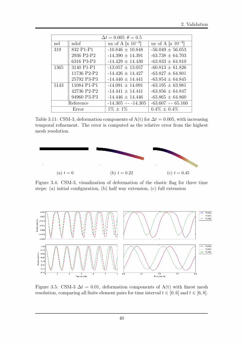
2. Validation
∆t = 0.005 θ = 0.5nel ndof ux of A [x 10−3] uy of A [x 10−3]319 832 P1-P1 -10.846 ± 10.848 -56.049 ± 56.053
2936 P2-P2 -14.390 ± 14.391 -63.738 ± 64.7036316 P3-P3 -14.429 ± 14.430 -63.833 ± 64.810
1365 3140 P1-P1 -13.057 ± 13.057 -60.813 ± 61.82611736 P2-P2 -14.426 ± 14.427 -63.827 ± 64.80125792 P3-P3 -14.440 ± 14.441 -63.854 ± 64.845
5143 11084 P1-P1 -14.091 ± 14.091 -63.195 ± 63.98142736 P2-P2 -14.441 ± 14.441 -63.856 ± 64.84794960 P3-P3 -14.446 ± 14.446 -63.865 ± 64.860
Reference -14.305 +- -14.305 -63.607 +- 65.160Error 1% ± 1% 0.4% ± 0.4%
Table 3.11: CSM-3, deformation components of A(t) for ∆t = 0.005, with increasingtemporal refinement. The error is computed as the relative error from the highestmesh resolution.
(a) t = 0 (b) t = 0.22 (c) t = 0.45
Figure 3.4: CSM-3, visualization of deformation of the elastic flag for three timesteps: (a) initial configuration, (b) half way extension, (c) full extension
Figure 3.5: CSM-3 ∆t = 0.01, deformation components of A(t) with finest meshresolution, comparing all finite element pairs for time interval t ∈ [0, 6] and t ∈ [6, 8].
40

Verification and Validation
Discussion
Comparing all finite-element pairs for CSM-3, visualized in figure 4.5, shows P2-P2and P3-P3 elements hardly can be distinguished from each other. In accordancewith previous mentioned results and observations, the solid solver is validated inaccordance with the validation benchmark.
3.2.4 Validation of fluid structure interaction solverThe validation of the FSI solver consist of three sub-problems which will be referredto FSI-1, FSI-2 and FSI-3. The FSI-1 problem yields a steady state solution forthe system, inducing small deformations to the elastic flag. The FSI-2 and FSI-3 problems results in a periodic solution, where the elastic flag oscillates behindthe cylinder. All sub-problems inherit the conditions from the previous validationbranches, with the exception of no gravitational force on the elastic flag. On thefluid-structure interface Γ, we enforce the kinematic and dynamic boundary condi-tion
vf = vs (3.5)σf · n = σs · n (3.6)
Apart from the accuracy of the reported values, the main purpose of the validationof the solver is twofold. First, it is of great importance to ensure that the overallcoupling of the fluid-structure interaction problem is executed correctly. Second,a good choice of mesh extrapolation model is essential to avoid divergence of thenumerical solution, due to mesh entanglement. Based on experience in section,4.2.1-2, the finite element pair P2-P1 for the fluid solver, and P2-P2 for the solidsolver proved successful. Therefore the finite-elements P2-P2-P1 for deformation,velocity, and pressure are chosen for the numerical experiments. Higher order el-ements will not be examined, mainly due to long computational time, even foroptimized solver approaches.
41
2. Validation
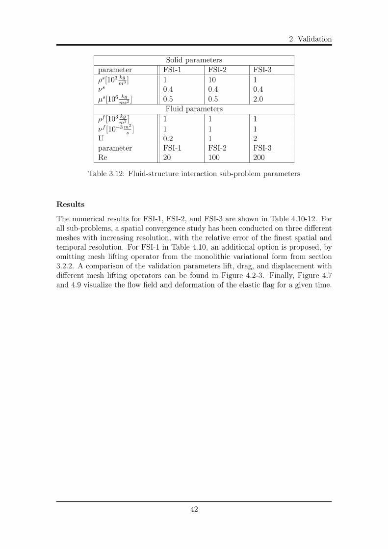
Solid parametersparameter FSI-1 FSI-2 FSI-3ρs[103 kg
m3 ] 1 10 1νs 0.4 0.4 0.4µs[106 kg
ms2] 0.5 0.5 2.0
Fluid parametersρf [103 kg
m3 ] 1 1 1νf [10−3m2
s] 1 1 1
U 0.2 1 2parameter FSI-1 FSI-2 FSI-3Re 20 100 200
Table 3.12: Fluid-structure interaction sub-problem parameters
Results
The numerical results for FSI-1, FSI-2, and FSI-3 are shown in Table 4.10-12. Forall sub-problems, a spatial convergence study has been conducted on three differentmeshes with increasing resolution, with the relative error of the finest spatial andtemporal resolution. For FSI-1 in Table 4.10, an additional option is proposed, byomitting mesh lifting operator from the monolithic variational form from section3.2.2. A comparison of the validation parameters lift, drag, and displacement withdifferent mesh lifting operators can be found in Figure 4.2-3. Finally, Figure 4.7and 4.9 visualize the flow field and deformation of the elastic flag for a given time.
42

Verification and Validation
FSI-1
Laplacenel ndof ux of A [x 10−3] uy of A [x 10−3] Drag Lift2474 21249 0.0226 0.8200 14.061 0.75427307 63365 0.0227 0.7760 14.111 0.751711556 99810 0.0226 0.8220 14.201 0.7609Reference 0.0227 0.8209 14.295 0.7638Error < 10−6 % < 10−6 % 0.66 % 0.38 %
Linear Elasticnel ndof ux of A [x 10−3] uy of A [x 10−3] Drag Lift2474 21249 0.0226 0.8198 14.061 0.75417307 63365 0.0227 0.7762 14.111 0.75111556 99810 0.0226 0.8222 14.201 0.7609Reference 0.0227 0.8209 14.295 0.7638Error < 10−6 % < 10−6 % 0.66 % 0.38 %
Biharmonic bc1nel ndof ux of A [x 10−3] uy of A [x 10−3] Drag Lift2474 21249 0.0226 0.8200 14.061 0.75417307 63365 0.0227 0.7761 14.111 0.751711556 99810 0.0227 0.8017 14.205 0.9248Reference 0.0227 0.8209 14.295 0.7638Error < 10−6 % < 10−6 % 0.63 % 21.08 %
Biharmonic bc2nel ndof ux of A [x 10−3] uy of A [x 10−3] Drag Lift2474 21249 0.0226 0.8200 14.061 0.75437307 63365 0.0227 0.7761 14.111 0.751811556 99810 0.0227 0.8020 14.205 0.9249Reference 0.0227 0.8209 14.295 0.7638Error < 10−6 % < 10−6 % 0.63 % 21.09 %
No extrapolationnel ndof ux of A [x 10−3] uy of A [x 10−3] Drag Lift2474 21249 0.0224 0.9008 14.064 0.77137307 63365 0.0226 0.8221 14.117 0.766011556 99810 0.0225 0.8787 14.212 0.7837Reference 0.0227 0.8209 14.295 0.7638Error < 10−6 % < 10−5 % 0.58 % 2.61 %
Table 3.13: FSI 1 - Comparison of mesh extrapolation models for three spatialrefinements
43

2. Validation
FSI-2
Laplace ∆t = 0.01 θ = 0.51nel ndof ux of A [x 10−3] uy of A [x 10−3] Drag Lift2474 21249 -15.27 ± 13.45 1.34 ± 82.4 157.00 ±14.85 -1.09 ±258.477307 63365 -14.23 ±13.37 1.31 ± 82.2 159,3 ± 15.43 0.92± 254.5311556 99810 -14.96 ± 13.24 1.28 ± 81.9 161.07 ± 17.81 0.02 ± 256.04
∆t = 0.001 θ = 0.5nel ndof ux of A [x 10−3] uy of A [x 10−3] Drag Lift2474 21249 -15.61± 13.21 1.34 ± 83.6 155.38 ± 13.98 -3.00 ± 289.067307 63365 -15.31 ± 13.07 1.02 ± 82.8 156.81 ± 14.95 -2.00 ± 276.2411556 99810 -15.28 ± 13.04 1.28 ± 82.9 158.45 ± 16.09 -2.53 ± 276.13Reference -14.58 ± 12.44 1.23 ±80.6 208.83 ± 73.75 0.88 ± 234.2Error (4.8 ± 4.8)10−6 % (4 ± 2.8) 10−6% 24.1 % ± 78.1 % 387.5 % ± 17.9 %
Biharmonic 1 ∆t = 0.01 θ = 0.51nel ndof ux of A [x 10−3] uy of A [x 10−3] Drag Lift2474 21249 -15.44 ± 13.24 -1.38 ± 82.3 157.67 ± 15.02 -0.89± 258.877307 63365 -15.04 ± 12.96 0.99 ± 81.9 159.83± 16.83 0.98 ± 245.4011556 99810 -15.29± 13.17 1.29 ± 82.5 161.69 ± 18.73 -1.86 ± 251.30
∆t = 0.001 θ = 0.5nel ndof ux of A [x 10−3] uy of A [x 10−3] Drag Lift2474 21249 -15.36 ± 13.12 1.35 ± 83.1 155.38 ± 13.74 -2.55 ± 285.197307 63365 -15.23 ± 12.97 1.03± 82.4 157.14 ± 15.18 -8.62 ± 263.8711556 99810 -15.27 ± 12.99 1.31 ± 82.7 157.72 ± 15.58 3.34 ± 258.76Reference -14.58 ± 12.44 1.23 ±80.6 208.83 ± 73.75 0.88 ± 234.2Error (4.7 ± 4.4)10−6 % (6.5 ± 2.6)10−6 % 208.83 ± 73.75 0.88 ± 234.2
Biharmonic 2 ∆t = 0.01 θ = 0.51nel ndof ux of A [x 10−3] uy of A [x 10−3] Drag Lift2474 21249 -14.93 ± 13.22 1.35 ± 81.5 157.76 ± 15.04 -0.49 ± 254.137307 63365 -14.67± 13.05 1.00± 80.9 159.59 ± 16.77 2.22 ± 248.1111556 99810 1.58 ± 12.86 1.23± 81.5 161.85 ±18.84 -1.64 ± 247.04
∆t = 0.001 θ = 0.5nel ndof ux of A [x 10−3] uy of A [x 10−3] Drag Lift2474 21249 -15.63 ± 12.7 1.31 ± 82.9 155.55 ± 13.82 -2.45 ± 281.187307 63365 -14,99 ± 12.81 0.99± 82.14 156.86 ± 15.05 -1.65 ± 269.8411556 99810 -15.26 ± 12.91 1.27 ± 81.8 156.86 ± 15.05 -1.65 ± 269.84Reference -14.58 ± 12.44 1.23 ±80.6 208.83 ± 73.75 0.88 ± 234.2Error (4.6 ± 3.7)10−6 % (3.2 ± 1.4)10−6 % 24.8 % ± 79.5 % 287.5 % ± 15.2 %
Table 3.14: FSI 1 - Comparison of mesh extrapolation models for ∆t = [0, 01, 0, 001],for three spatial refinements
44
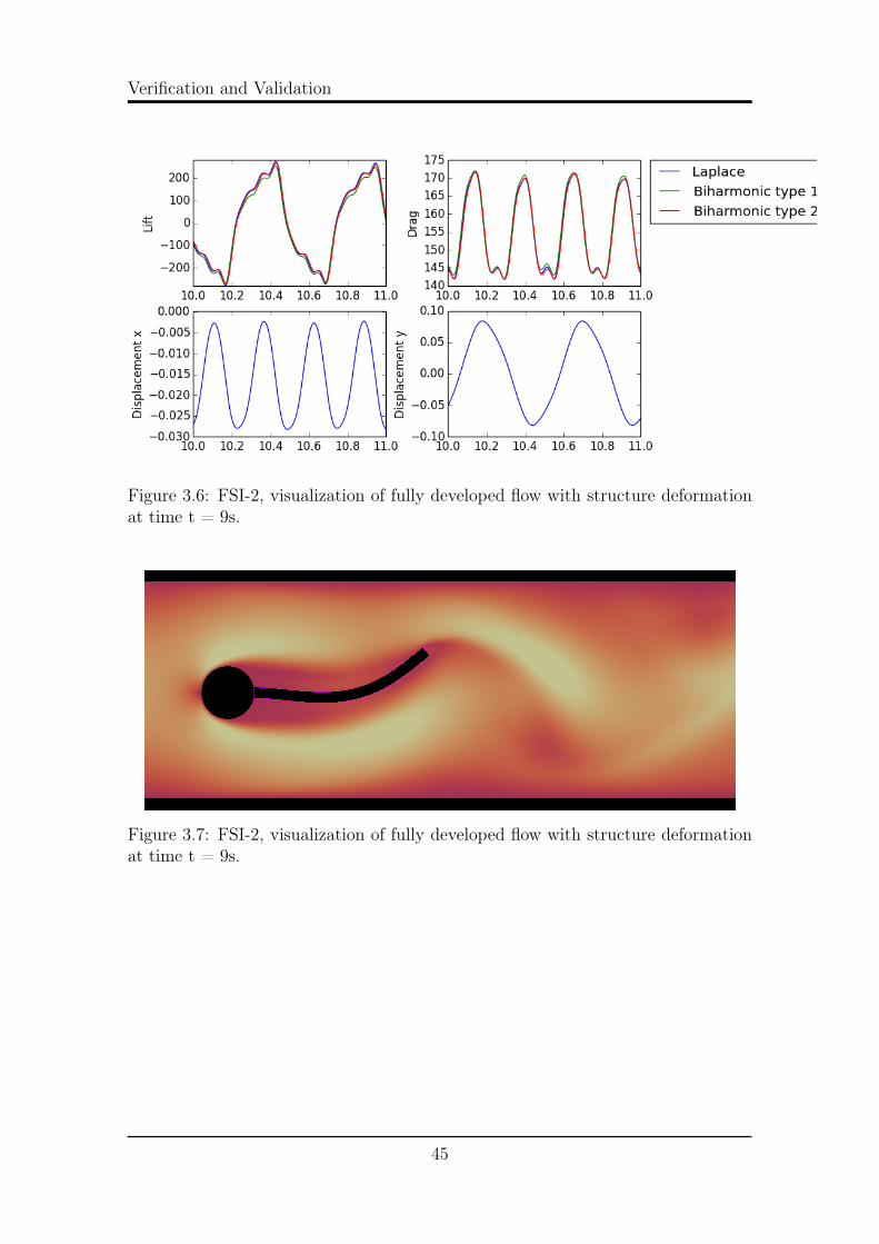
Verification and Validation
Figure 3.6: FSI-2, visualization of fully developed flow with structure deformationat time t = 9s.
Figure 3.7: FSI-2, visualization of fully developed flow with structure deformationat time t = 9s.
45

2. Validation
FSI-3
Table 3.15: FSI 3 - Comparison of mesh extrapolation models
Laplace ∆t = 0.01θ = 0.51nel ndof ux of A [x 10−3] uy of A [x 10−3] Drag Lift2474 21249 -2.41 ± 2.41 1.49 ± 32.21 449.39 ± 14.72 0.55 ± 155.807307 63365 -2.32 ± 2.31 1.32 ± 31.80 451.76 ± 16.10 1.04 ± 151.5111556 99810 -2.34 ± 2.34 1.59 ± 31.91 455.94 ± 17.34 -0.01 ± 151.36
∆t = 0.001θ = 0.5nel ndof ux of A [x 10−3] uy of A [x 10−3] Drag Lift2474 21249 -2.91 ± 2.74 1.28 ± 35.01 450.90 ± 18.11 2.28 ±161.137307 63365 -2.82 ± 2.66 1.24 ± 34.69 453.56 ± 19.80 2.94 ± 158.6711556 99810 -2.88 ± 2.72 1.49 ± 34.97 458.60 ± 22.12 2.23 ± 158.95Reference -2.69 ± 2.56 1.48 ± 34.38 457.3 ± 22.66 2.22 ± 149.78Error (7.0 ± 6.2)10−6 % (6.7 ± 1.7)10−6 % 0.28 % ± 2.38 % 0.45 % ± 6.12 %
Biharmonic 1 ∆t = 0.01θ = 0.51nel ndof ux of A [x 10−3] uy of A [x 10−3] Drag Lift2474 21249 -2.40 ± 2.38 1.58 ± 32.07 450.16 ± 15.11 -20.09 ± 148.177307 63365 -2.26 ± 2.14 1.70 ± 31.3 457.37 ± 15.24 -51.77 ± 127.2811556 99810 -2.33 ± 2.32 1.93 ± 31.5 456.40 ± 17.45 0.45 ± 149.68
∆t = 0.001θ = 0.5nel ndof ux of A [x 10−3] uy of A [x 10−3] Drag Lift2474 21249 -2.18 ± 2.10 3.52 ± 2.90 435.19 ± 9.77 -1.59± 151.457307 63365 -2.80 ± 2.64 1.25 ± 3.45 454.38 ± 19.76 17.97 ± 155.0811556 99810 -2.84 ± 2.68 1.50 ± 3.47 459.12 ± 22.97 -3.12 ± 171.22Reference -2.69 ± 2.56 1.48 ± 34.38 457.3 ± 22.66 2.22 ±- 149.78Error (5.5 ± 4.6)10−6 % (1.3 ± 8.9)10−6 % 0.40 % ± 1.37 % 240.5 % ± 14.3 %
Biharmonic 2 ∆t = 0.01θ = 0.51nel ndof ux of A [x 10−3] uy of A [x 10−3] Drag Lift2474 21249 -2.33 ± 2.33 1.57 ± 31.6 449.44 ± 14.82 0.80 ±152.037307 63365 -2.25 ± 2.23 1.35 ± 31.3 452.63 ±16.29 17.11 ± 146.0511556 99810 -2.25 ± 2.29 1.59 ± 31.4 457.89 ± 17.26 57.83 ± 141.69
∆t = 0.001θ = 0.5nel ndof ux of A [x 10−3] uy of A [x 10−3] Drag Lift2474 21249 -2.83 ± 2.66 1.31 ± 34.5 450.24 ± 18.25 2.57 ± 175.427307 63365 -2.77 ± 2.61 0.98± 34.6 453.53 ± 20.01 2.60 ± 159.1311556 99810 -2.80 ± 2.65 1.37 ± 34.7 458.41 ± 22.23 15.56 ± 157.78Reference -2.69 ± 2.56 1.48 ± 34.38 457.3 ± 22.66 2.22 ±- 149.78Error (4.0 ± 3.5)10−6 % (7.4 ± 9.3)10−6 % 0.24 % ± 1.90 % 600.9 % ± 5.34 %
46

Verification and Validation
Figure 3.8: Comparison of mesh motion models for FSI-3, in time interval t t ∈[5.5, 6].
Figure 3.9: FSI-3, visualization of fully developed flow with structure deformationat time t = 5.1s.
47
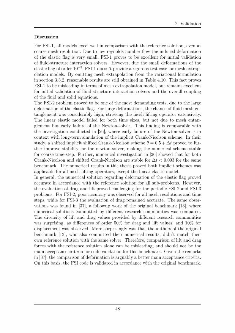
2. Validation
Discussion
For FSI-1, all models excel well in comparison with the reference solution, even atcoarse mesh resolution. Due to low reynolds number flow the induced deformationof the elastic flag is very small, FSI-1 proves to be excellent for initial validationof fluid-structure interaction solvers. However, due the small deformations of theelastic flag of order 10−5, FSI-1 doesn’t provide a rigorous test case for mesh extrap-olation models. By omitting mesh extrapolation from the variational formulationin section 3.3.2, reasonable results are still obtained in Table 4.10. This fact provesFSI-1 to be misleading in terms of mesh extrapolation model, but remains excellentfor initial validation of fluid-structure interaction solvers and the overall couplingof the fluid and solid equations.The FSI-2 problem proved to be one of the most demanding tests, due to the largedeformation of the elastic flag. For large deformations, the chance of fluid mesh en-tanglement was considerably high, stressing the mesh lifting operator extensively.The linear elastic model failed for both time sizes, but not due to mesh entan-glement but early failure of the Newton-solver. This finding is comparable withthe investigation conducted in [26], where early failure of the Newton-solver is incontext with long-term simulation of the implicit Crank-Nicolson scheme. In theirstudy, a shifted implicit shifted Crank-Nicolson scheme θ = 0.5 + ∆t proved to fur-ther improve stability for the newton-solver, making the numerical scheme stablefor coarse time-step. Further, numerical investigation in [26] showed that for bothCrank-Nicolson and shifted Crank-Nicolson are stable for ∆t < 0.003 for the samebenchmark. The numerical results in this thesis proved both implicit schemes wasapplicable for all mesh lifting operators, except the linear elastic model.In general, the numerical solution regarding deformation of the elastic flag provedaccurate in accordance with the reference solution for all sub-problems. However,the evaluation of drag and lift proved challenging for the periodic FSI-2 and FSI-3problems. For FSI-2, poor accuracy was observed for all mesh resolutions and timesteps, while for FSI-3 the evaluation of drag remained accurate. The same obser-vations was found in [37], a followup work of the original benchmark [13], wherenumerical solutions committed by different research communities was compared.The diversity of lift and drag values provided by different research communitieswas surprising, as differences of order 50% for drag and lift values, and 10% fordisplacement was observed. More surprisingly was that the authors of the originalbenchmark [13], who also committed their numerical results, didn’t match theirown reference solution with the same solver. Therefore, comparison of lift and dragforces with the reference solution alone can be misleading, and should not be themain acceptance criteria for code validation for this benchmark. Given the remarksin [37], the comparison of deformation is arguably a better main acceptance criteria.On this basis, the FSI code is validated in accordance with the original benchmark.
48

Numerical Experiments
4.1 Comparison of mesh lifting operators
Mesh lifting operators are essential for numerical stability of fluid-structure inter-action. If the fluid mesh doesn’t conform with the solid deformation, mesh entan-glement increases with the possibility of numerical instabilities. In general, meshmodels have shown to be either robust concerning mesh entanglements at the cost ofcomputational time, or computational efficient with less robustness [19]. However,computational efficiency has proven not only to be dependent of the complexity ofmodel, but also the regularity of the fluid mesh, reducing Newton iterations neededper time step [41]. In this section, a comparison of the mesh lifting operators fromsection 3.1.4. for the FSI-3 benchmark are presented. The linear elastic model wasfound not applicable in section 4.2.3. Therefore, only the Laplace and biharmoniclifting operators will be considered, comparing vertical displacement of the elasticflag, regularity of the fluid mesh, and number of Newton iterations per time step.To evaluate the regularity of the fluid mesh, the minimum value of the Jacobianof the deformation gradient have been considered in [41]. The Jacobian serves asa measure of mesh entanglement, meaning if Jf ≥ 0, there are no crossing cells inthe fluid mesh.
Jf = det(Ff ) = det(I + ∇uf )
where I is the identity matrix and uf is the fluid mesh deformation.
49

1. Comparison of mesh lifting operators
ResultsFigure 4.1 shows a comparison the mesh lifting operators at the time interval t =[0, 5], when a stable periodic solution is obtained. As shown in the middle figureall models shows a minima of mesh regularity at 3.8s < t < 4.2, which is expecteddue to the largest deformation of the elastic flag. A larger number of Newtoniterations for all models shows are needed at each time step, when the elastic flagstarts oscillating for t > 3s. The biharmonic lifting operator is superior in terms ofnumber of iterations need per time step, and mesh regularity in comparison with theLaplace model. Further, the biharmonic 2 model shows better mesh regularity thanbiharmonic 1, but shows equal behavior in terms of Newton iterations. Recall, thebiharmonic 2 operator allows tangential mesh motion at the boundaries, while thebiharmonic 1 model constraining mesh motion in both perpendicular and tangentialdirection. For all models, no distinct difference in deformation of the y-componentis found.
Figure 4.1: Investigation of mesh lifting operators for the FSI3 benchmark in thetime interval t ∈ [0, 5], comparing vertical displacement of elastic flag, mesh regu-larity, and number of Newton iterations.
DiscussionThe numerical results confirms biharmonic models produce a better regularity ofthe fluid mesh cells, which in turn reduces the number of Newton iterations neededper time step. However, better evolution of mesh cells is by no means necessary forsolving the FSI-3 problem. Therefore, the Laplace model remains a good choice, andits simplicity is preferable in terms of computational time (a topic to be discussedin section 4.2 4.3 ).
50
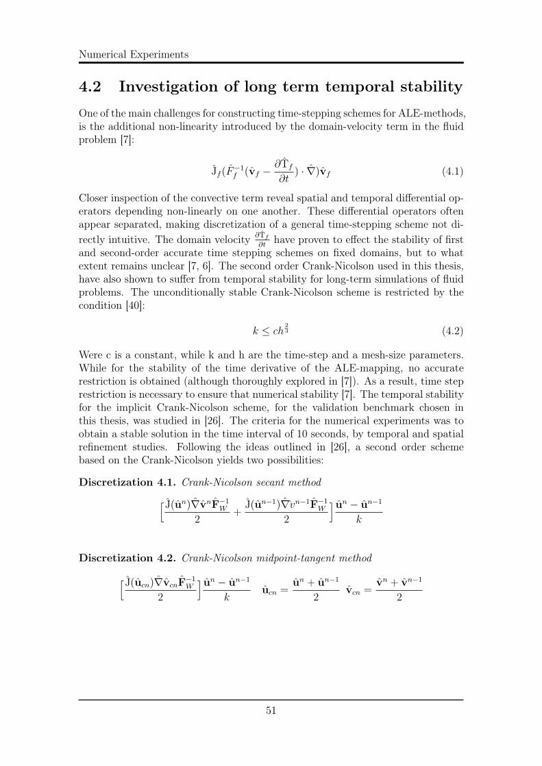
Numerical Experiments
4.2 Investigation of long term temporal stability
One of the main challenges for constructing time-stepping schemes for ALE-methods,is the additional non-linearity introduced by the domain-velocity term in the fluidproblem [7]:
Jf (F−1f (vf −
∂Tf
∂t) · ∇)vf (4.1)
Closer inspection of the convective term reveal spatial and temporal differential op-erators depending non-linearly on one another. These differential operators oftenappear separated, making discretization of a general time-stepping scheme not di-rectly intuitive. The domain velocity ∂Tf
∂thave proven to effect the stability of first
and second-order accurate time stepping schemes on fixed domains, but to whatextent remains unclear [7, 6]. The second order Crank-Nicolson used in this thesis,have also shown to suffer from temporal stability for long-term simulations of fluidproblems. The unconditionally stable Crank-Nicolson scheme is restricted by thecondition [40]:
k ≤ ch23 (4.2)
Were c is a constant, while k and h are the time-step and a mesh-size parameters.While for the stability of the time derivative of the ALE-mapping, no accuraterestriction is obtained (although thoroughly explored in [7]). As a result, time steprestriction is necessary to ensure that numerical stability [7]. The temporal stabilityfor the implicit Crank-Nicolson scheme, for the validation benchmark chosen inthis thesis, was studied in [26]. The criteria for the numerical experiments was toobtain a stable solution in the time interval of 10 seconds, by temporal and spatialrefinement studies. Following the ideas outlined in [26], a second order schemebased on the Crank-Nicolson yields two possibilities:
Discretization 4.1. Crank-Nicolson secant method[ J(un)∇vnF−1W
2+
J(un−1)∇vn−1F−1W
2
] un − un−1
k
Discretization 4.2. Crank-Nicolson midpoint-tangent method[ J(ucn)∇vcnF−1W
2
] un − un−1
kucn =
un + un−1
2vcn =
vn + vn−1
2
51

2. Investigation of long term temporal stability
The numerical experiments showed very similar performance for discretization 4.1,4.2, and significant differences of long-term temporal stability was not found. How-ever, spatial and temporal refinement showed the implicit Crank-Nicolson sufferedfrom long-term stability problems for certain time steps. Choosing the time stepk = [0.005, 0.003], the FSI-3 problem (section 3.2.4 ) suffered from numerical in-stabilities. Interestingly, the instabilities occurred earlier in simulation time forincreasing mesh refinement. A similar experiment in [43], showed reducing the timestep k = 0.001 yield stable long-time simulation for both Discretization 4.1 and4.2.To overcomes the numerical instabilities two approaches have been suggested in theliterature, the shifted Crank-Nicolson and the frac-step method [26, 43, 40]. In thisthesis the shifted Crank-Nicolson scheme was considered, introducing stability tothe overall system by shifting the centered scheme by θ = 1
2+ k. If the shift is
dependent of the time-step k such that 12≤ θ ≤ 1
2+ k, the scheme will be of second
order [26].
ResultsA numerical investigation of long term numerical stability is shown in Figure 4.2,4.3, where the shifted Crank-Nicolson scheme θ = 1
2+ ∆t, is compared the orig-
inal Crank-Nicolson θ = 12. The shifted surpasses the original Crank-Nicolson
scheme in terms of temporal stability, for all time steps. In Figure 4.3, the shiftedCrank-Nicholson scheme retain long-time temporal stability for ∆t = 0.01.. Whilefor the ordinary Crank-Nicholson scheme, numerical experiments showed choosing∆t = 0.001 was necessarily to ensure stability, confirming the results found in [43].Figure 4.2 shows choosing ∆t ∈ [0.2, 0.1] results in a steady-state solution, whichcan be explained by influence the solid problem. A centered Crank-Nicolson schemeθ = 1
2is energy preserving, meaning no energy is dissipated from the system. Since
the shifted Crank-Nicolson scheme is not centered, the amount of dissipated ofenergy is related to the time step. If the time step is sufficiently high such as∆t ∈ [0.2, 0.1], the scheme will dissipate energy at a higher rate. Therefore, noperiodic oscillation of the elastic flag is obtained. The validation of the solid solvershows the difference of energy dissipation for a centered and backward numericalscheme. Given the same solid parameters, a steady-state solution is obtained forCSM-1 (θ = 1.0), while CSM-3 yields a periodic solution CSM-3 (θ = 1
2), shown in
Figure 4.4 .For ∆t ∈ [0.05, 0.02], the shifted Crank-Nicolson scheme is close to centered, mean-ing energy is nearly preserved in the structure. However, the Newton-solver di-verges before full time interval of 10 seconds is finished. Surprisingly, a finer timestep ∆t = 0.02 fails at an earlier stage than ∆t = 0.05. The numerical divergenceis not due to mesh entanglement of the ALE-mapping, but divergence of Newtonmethod itself [26]. It is believed the divergence of the Newton solver is linked tothe influence of the domain velocity, by the research found in [7], but no clear timestep restriction is obvious. Hence, several publications indicates choosing time stepfor a shifted Crank-Nicolson scheme is based on trial and error [43, 40].
52

Numerical Experiments
Figure 4.2: Investigation of long term numerical stability for the FSI3 benchmarkin the time interval t ∈ [0, 10], comparing the shifted and centered Crank-Nicolsonscheme.
Figure 4.3: Investigation of long term numerical stability for the FSI3 benchmarkin the time interval t ∈ [0, 10], comparing the shifted and centered Crank-Nicolsonscheme.
4.3 Optimization of the Newton solver
Software profiling is a dynamic program analysis, with the purpose of finding soft-ware sections which can be optimized. In scientific computing, software profilingoften focuses on minimizing memory usage or executing speed, by collecting per-formance data to identify bottlenecks. A bottleneck is a term used when the totalperformance of a complete implementation is limited to small code fragments, ac-counting for the primary consumption of computer resources. For many applica-tions, one can often assume the usage of resources follows the The Pareto principle.Meaning that for different types of events, roughly 80% of the effects come from20% of the causes. An analogy to computational sciences it that 80% of the compu-
53
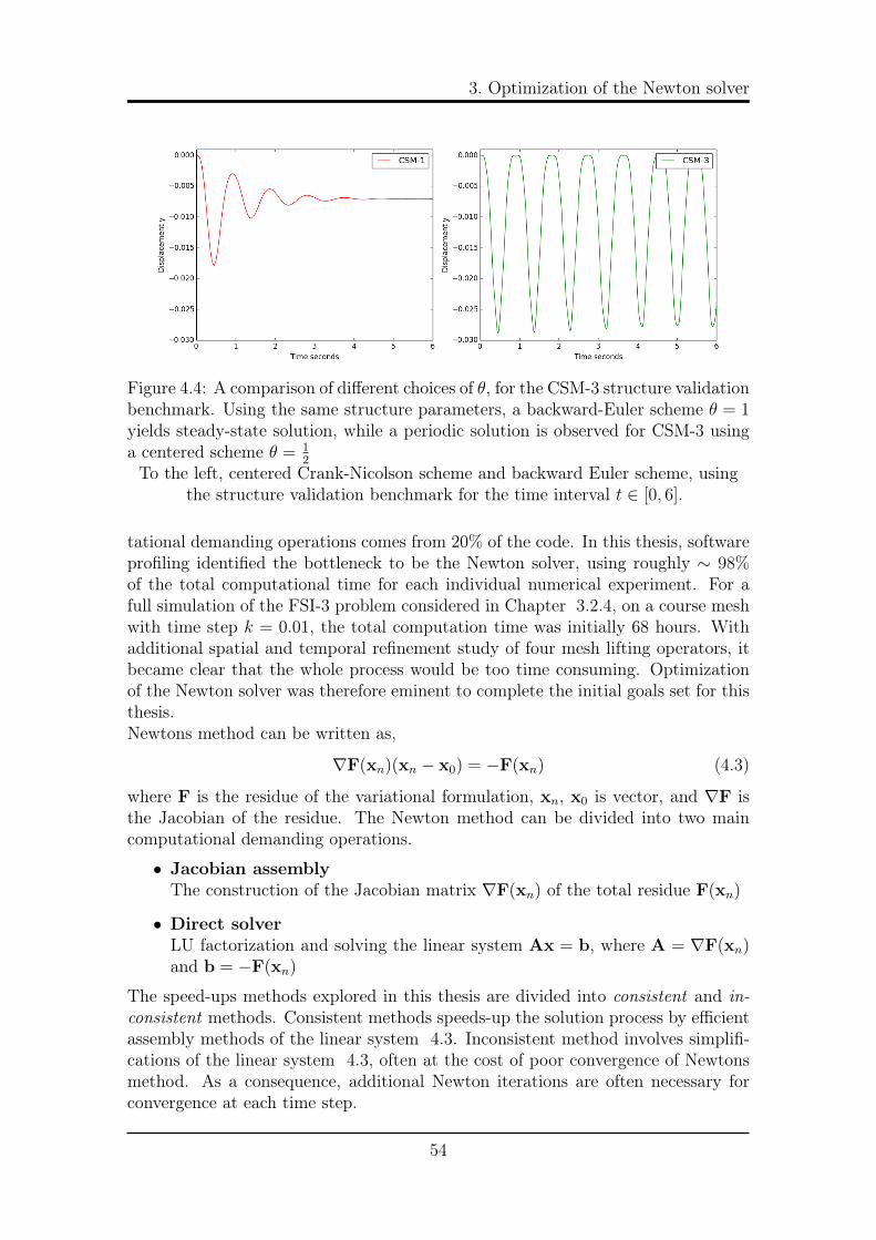
3. Optimization of the Newton solver
Figure 4.4: A comparison of different choices of θ, for the CSM-3 structure validationbenchmark. Using the same structure parameters, a backward-Euler scheme θ = 1yields steady-state solution, while a periodic solution is observed for CSM-3 usinga centered scheme θ = 1
2
To the left, centered Crank-Nicolson scheme and backward Euler scheme, usingthe structure validation benchmark for the time interval t ∈ [0, 6].
tational demanding operations comes from 20% of the code. In this thesis, softwareprofiling identified the bottleneck to be the Newton solver, using roughly ∼ 98%of the total computational time for each individual numerical experiment. For afull simulation of the FSI-3 problem considered in Chapter 3.2.4, on a course meshwith time step k = 0.01, the total computation time was initially 68 hours. Withadditional spatial and temporal refinement study of four mesh lifting operators, itbecame clear that the whole process would be too time consuming. Optimizationof the Newton solver was therefore eminent to complete the initial goals set for thisthesis.Newtons method can be written as,
∇F(xn)(xn − x0) = −F(xn) (4.3)
where F is the residue of the variational formulation, xn, x0 is vector, and ∇F isthe Jacobian of the residue. The Newton method can be divided into two maincomputational demanding operations.
• Jacobian assemblyThe construction of the Jacobian matrix ∇F(xn) of the total residue F(xn)
• Direct solverLU factorization and solving the linear system Ax = b, where A = ∇F(xn)and b = −F(xn)
The speed-ups methods explored in this thesis are divided into consistent and in-consistent methods. Consistent methods speeds-up the solution process by efficientassembly methods of the linear system 4.3. Inconsistent method involves simplifi-cations of the linear system 4.3, often at the cost of poor convergence of Newtonsmethod. As a consequence, additional Newton iterations are often necessary forconvergence at each time step.
54

Numerical Experiments
4.3.1 Consistent methods
Jacobi buffering
The residue of the FSI problem consists of both linear and non-linear terms, F =Flin + Fnonlin. For each time step the linear part Flin remains constant, whichonly need to be assembled on the first Newton iteration. The linear parts arethen buffered, meaning saved in a separate matrix and added with the assemblednon-linear Fnonlin matrix for each Newton iteration at each time step.
4.3.2 Inconsistent methods
Reuse of Jacobian
Reusing the Jacobian of the residue∇F(xn) have two beneficial consequences. First,the Jacobian of the residue ∇F(xn) is only assembled once at each time step.Second, the LU factorization of the linear system 4.3 is only needed at the firstiteration, as the Jacobian remains constant through the whole time step. The firstNewton iteration is therefore solved without simplifications, while the remainingiterations uses an inexact Jacobian which reduces the convergence of the method.
Quadrature reduce
The assemble time of the Jacobian greatly depends on the degree of polynomialsused in the discretization of the total residual. The use of lower order polynomialsreduces assemble time of the Jacobian at each Newton iteration due decreased size ofthe Jacobian matrix. The decreased size of the matrix also reduces the time neededfor LU-factorization of the linear system 4.3. However, the quadrature reducemethod leads to an inexact Jacobian which may results to additional iterations.
Combining quadrature reduce and Jacobian reuse
By using the previous inconsistent methods together, the first assembly of the Jaco-bian is done with lower order polynomials. This combination reduces assembly timeof the Jacobian matrix at first iteration, and further speeds up LU-factorization ofthe linear system 4.3.
4.3.3 Comparison of speedup methods
In Figure 4.5, all speed-up techniques are compared on the time interval t = [0, 5],for the Laplacian model. Numerical simulations shows how all inconsistent methodsincrease the number of iterations needed for convergence at each time step, contraryto a consistent naive method. However, the inconsistent methods clearly dominatethe time used for a full Newton iteration at each time step, in comparison withthe naive approach. The fastest method proved to be the combined method, using1.5 hours for solving the full time interval. The naive approach used 17.1 hours,meaning the combined method resulted in a 91% speedup.
55
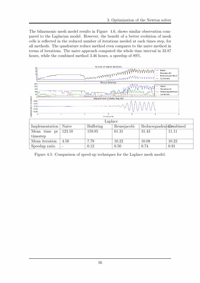
3. Optimization of the Newton solver
The biharmonic mesh model results in Figure 4.6, shows similar observation com-pared to the Laplacian model. However, the benefit of a better evolution of meshcells is reflected in the reduced number of iterations needed at each times step, forall methods. The quadrature reduce method even compares to the naive method interms of iterations. The naive approach computed the whole time interval in 33.87hours, while the combined method 3.46 hours, a speedup of 89%.
LaplaceImplementation Naive Buffering Reusejacobi ReducequadratureCombinedMean time prtimestep
123.10 159.85 61.31 31.43 11.11
Mean iteration 4.50 7.79 10.22 10.08 10.22Speedup ratio - 0.12 0.50 0.74 0.91
Figure 4.5: Comparison of speed-up techniques for the Laplace mesh model.
56

Numerical Experiments
Biharmonic Type 1Implementation Naive Buffering Reusejacobi Reducequad CombinedMean time prtimestep
243.39 307.67 76.77 51.64 24.87
Mean iteration 4.14 6.21 7.19 4.67 6.81Speedup ration - -0.26 0.68 0.79 0.90
Figure 4.6: Comparison of speed-up techniques for the biharmonic type 1 meshmodel.
Discussion
Of the speed-up methods considered in this thesis, the combined method proved tofastest for both mesh models. With a computational time difference of nearly ∼ 2hours, the Laplace model is superior to the biharmonic model in terms of efficiency.As long as mesh regularity isn’t critical for the simulation, the Laplacian model isthe preferable lifting operator. It is important to note that the introduced speed-up methods may not be applicable to other FSI problems, since inexact Jacobianmethods are highly sensitive.
57

3. Optimization of the Newton solver
58
Conclusion and further research
In this thesis, a monolithic fluid-structure interaction solver in an arbitrary La-grangian Eulerian description have been presented. This inline with the originalgoal of this thesis. However, verification of code was not achieved, however suc-cessful validation through the benchmark presented in [13] indicates the code stillrepresents the mathematical model correctly enough. Thus it opens up the possi-bility that the verification of code test it self might have been erroneous.
An investigation of long term temporal stability of the FSI benchmark showed theimplicit Crank-Nicolson was not applicable for time steps ∆t > 0.001. To overcomethe stability issues, a shifted Crank-Nicolson scheme was introduced, were long timetemporal stability was obtained for ∆t ≤ 0.01. Software profiling motivated run-time optimizations of the Newton solver, where a combination of Jacobian reuse andlower-order polynomials to assemble the Jacobian matrix proved most beneficial interms of computational efficiency.
In order to further explore all aspects of the FSI problem, I have also compared threedifferent mesh lifting operators, focusing on mesh regularity and computational ef-ficiency. The Laplace lifting operator proved to be the most efficient method, whilethe biharmonic operator was the most rigorous, however at the cost of computa-tional cost. The linear elastic model failed for all tests expect the FSI-1 problem,meaning it was only valid for small deformations.
59

Future researchTo pursue a successful verification of code is the primary future goal, which is neces-sary remove any doubt that the mathematical model is solved correctly. In addition,several extensions are possible. Several publications have showed the linear elas-tic lifiting operator applicable for a wide range of FSI problems. Therefore, furtherinvestigation is planned to investigate why the operator did not perform in my work.
Hoping to extend into 3D simulations, an implementation of iterative Krylov meth-ods by block preconditioning are necessary, to overcome the CPU demanding natureof the monolithic FSI formulation. A substantial amount of time during the workof this thesis have been put into trying to implement the partitioned algorithm pre-sented in [5]. In the end, I was not able to finalize this project, but future researchwill be spent on finding the last mistakes. A projection method would allow for awider variety of fluid schemes, making the whole fluid equation linear. Thus, havingthe potential of further speeding up the solution process.
60

Appendices
61

The deformation gradient
Deformation is a major property of interest when a continuum is influenced by ex-ternal and internal forces. The deformation results in relative change of position ofmaterial particles, called strain, is the primary property that causes and describestress. Strain is purely an observation, not dependent on the material of interest.However one expects that a material undergoing strain, will apply forces within dueto neighboring material particles interacting with one another. Therefore, materialspecific models are derived to describe how a certain material will react to a certainamount of strain. Strain measures are used to define models for stress, which isresponsible for the deformation in materials [12]. Stress is defined as the internalforces that particles within a continuous material exert on each other, with dimen-sion force per unit area.The equations of continuum mechanics can be derived with respect to either a de-formed or undeformed configuration. The choice of referring our equations to thecurrent or reference configuration is indifferent from a theoretical point of view.Regardless of configuration, the deformation gradient and determinant of the de-formation gradient are essential measurement in structure mechanics. By [25], bothconfigurations are considered.
Reference configuration
Definition A.1. Let u be a differential deformation field in the reference config-uration, I be the Identity matrix and the gradient ∇ = ( ∂
∂x, ∂∂y, ∂∂z
). Then thedeformation gradient is given by,
F = I + ∇u (A.1)
expressing the local change of relative position under deformation.
Definition A.2. Let u be a differential deformation field in the reference config-uration, I be the Identity matrix and the gradient ∇ = ( ∂
∂x, ∂∂y, ∂∂z
). Then thedeterminant of the deformation gradient is given by,
J = det(F) = det(I + ∇u) (A.2)
expressing the local change of volume of the configuration.
63
Current configuration
Definition A.3. Let u be a differential deformation field in the reference config-uration, I be the Identity matrix and the gradient ∇ = ( ∂
∂x, ∂∂y, ∂∂z
). Then thedeformation gradient is given by,
F = I −∇u (A.3)
Definition A.4. Let u be a differential deformation field in the reference config-uration, I be the Identity matrix and the gradient ∇ = ( ∂
∂x, ∂∂y, ∂∂z
). Then thedeterminant of the deformation gradient is given by,
J = det(F) = det(I −∇u) (A.4)
64
Bibliography
[1] Robert Biedron and Elizabeth Lee-Rausch. Rotor Airloads Prediction UsingUnstructured Meshes and Loose CFD/CSD Coupling. In 26th AIAA AppliedAerodynamics Conference, pages 2–3, Reston, Virigina, aug 2008. AmericanInstitute of Aeronautics and Astronautics.
[2] P Crumpton and M Giles. Implicit time accurate solutions on unstructureddynamic grids. Numerical methods in Fluids, 25(11):1285–1300, jun 1997.
[3] J Donea, A Huerta, J.-Ph Ponthot, and A Rodríguez-Ferran. ArbitraryLagrangian-Eulerian methods. (1969):1–38, 2004.
[4] Miguel A Fernández and Jean-Frédéric Gerbeau. Algorithms for fluid-structureinteraction problems. 2009.
[5] Miguel A. Fernández, Jean Frederic Gerbeau, and Ceremade Grandmont. Aprojection semi-implicit scheme for the coupling of an elastic structure withan incompressible fluid. International Journal for Numerical Methods in En-gineering, 69(4):794–821, 2007.
[6] L Formaggia and F Nobile. A stability analysis for the arbitrary LagrangianEulerian formulation with finite elements. East-west journal of numerical math-ematics, Vol. 7(No. 2):105–131, 1991.
[7] Luca Formaggia and Fabio Nobile. Stability analysis of second-order timeaccurate schemes for ALE-FEM. Computer Methods in Applied Mechanicsand Engineering, 193(39-41 SPEC. ISS.):4097–4116, 2004.
[8] Christiane Förster, Wolfgang A. Wall, and Ekkehard Ramm. Artificial addedmass instabilities in sequential staggered coupling of nonlinear structures andincompressible viscous flows. Computer Methods in Applied Mechanics andEngineering, 196(7):1278–1293, 2007.
[9] S. Frei, T. Richter, and T. Wick. Long-term simulation of large deformation,mechano-chemical fluid-structure interactions in ALE and fully Eulerian coor-dinates. Journal of Computational Physics, 321:874–891, 2016.
[10] Bernhard Gatzhammer. Efficient and Flexible Partitioned Simulation of Fluid-Structure Interactions. PhD thesis, Technische Universit¨at Munchen, 2014.
65

BIBLIOGRAPHY
[11] Brian T. Helenbrook. Mesh deformation using the biharmonic operator. In-ternational Journal for Numerical Methods in Engineering, 2003.
[12] Gerhard A. Holzapfel. Nonlinear Solid Mechanics: A Continuum Approach forEngineering. John Wiley og Sons Ltd, 2000.
[13] Jaroslav Hron and Stefan Turek. Proposal for numerical benchmarking of fluid-structure interaction between an elastic object and laminar incompressible flow.Fluid-Structure Interaction, 53:371–385, 2006.
[14] Su-Yuen Hsu, Chau-Lyan Chang, and Jamshid Samareh. A Simplified MeshDeformation Method Using Commercial Structural Analysis Software. In 10thAIAA/ISSMO Multidisciplinary Analysis and Optimization Conference, pages2–5, Reston, Virigina, aug 2004. American Institute of Aeronautics and Astro-nautics.
[15] Jay D. Humphrey. Cardiovascular Solid Mechanics. Springer New York, NewYork, NY, 2002.
[16] Hrvoje Jasak and Željko Tuković. Automatic mesh motion for the unstructuredFinite Volume Method. Transactions of Famena, 30(2):1–20, 2006.
[17] V V Meleshko. Bending of an Elastic Rectangular Clamped Plate: ExactVersus ’Engineering’ Solutions. Journal of Elasticity, 48(1):1–50, 1997.
[18] José Merodio and Giuseppe Saccomandi. Continuum Mechanics - Volume I.In Volume 1, chapter 3, pages 82–84. EOLSS, 2011.
[19] Selim MM and Koomullil RP. Mesh Deformation Approaches – A Survey.Journal of Physical Mathematics, 7(2), 2016.
[20] J Newman. Marine Hydrodynamics. 1977.
[21] William L. Oberkampf and Christopher J. Roy. Verification and Validation inScientific Computing. Cambridge University Press, Cambridge, 2010.
[22] M Razzaq, Stefan Turek, Jaroslav Hron, J F Acker, F Weichert, I Grunwald,C Roth, M Wagner, and B Romeike. Numerical simulation and benchmarkingof fluid-structure interaction with application to Hemodynamics. FundamentalTrends in Fluid-Structure Interaction, 1:171–199, 2010.
[23] T Richter. Numerical Methods for Fluid-Structure Interaction Problems.Course of lectures, 2010(August 2010), 2010.
[24] T. Richter and T. Wick. Finite elements for fluid-structure interaction in ALEand fully Eulerian coordinates. Computer Methods in Applied Mechanics andEngineering, 199(41-44):2633–2642, 2010.
[25] Thomas Richter. Fluid Structure Interactions. 2016.
66
BIBLIOGRAPHY
[26] Thomas Richter and ThomasWick. On Time Discretizations of Fluid-StructureInteractions. pages 377–400. 2015.
[27] Patrick J. Roache. Code Verification by the Method of Manufactured Solutions.Journal of Fluids Engineering, 124(1):4, 2002.
[28] P.J. Roache. Verification and Validation in Computational Science and En-gineering. Computing in Science Engineering, Hermosa Publishers, 1998, 8-9,1998.
[29] Edward J. Rykiel. Testing ecological models: The meaning of validation. Eco-logical Modelling, 90(3):229–244, 1996.
[30] Kambiz Salari and Patrick Knupp. Code Verification by the Method of Man-ufactured Solution. Technical report, Sandia National Laboratories, 2000.
[31] LE Schwer. Guide for verification and validation in computational solid me-chanics. American Society of Mechanical Engineers, PTC 60(V&V 10):1–15,2006.
[32] Jason P Sheldon, Scott T Miller, and Jonathan S Pitt. Methodology for Com-paring Coupling Algorithms for Fluid-Structure Interaction Problems. WorldJournal of Mechanics, 4(February):54–70, 2014.
[33] J.C. Simo and F. Armero. Unconditional stability and long-term behavior oftransient algorithms for the incompressible Navier-Stokes and Euler equations.Computer Methods in Applied Mechanics and Engineering, 111(1-2):111–154,jan 1994.
[34] Ian Sommerville. Verification and Validation Benchmarks. Technical ReportFebruary, Sandia National Laboratories, 2006.
[35] K Stein, T Tezduyar, and R Benney. Mesh Moving Techniques for Fluid-Structure Interactions With Large Displacements. Journal of applied mechan-ics, 70(1):58–63, 2003.
[36] Dominique Tremblay, Stephane Etienne, and Dominique Pelletier. Code Ver-ification and the Method of Manufactured Solutions for Fluid-Structure In-teraction Problems. In 36th AIAA Fluid Dynamics Conference and Exhibit,number June, pages 1–11, Reston, Virigina, jun 2006. American Institute ofAeronautics and Astronautics.
[37] Stefan Turek, Jaroslav Hron, Mudassar Razzaq, and Hilmar Wobker. Numer-ical Benchmarking of Fluid-Structure Interaction : A comparison of differentdiscretization and solution approaches.
[38] Wolfgang A. Wall, Axel , Gerstenberger, Peter , Gamnitzer, Christiane ,Förster, and Ekkehard , Ramm. Large Deformation Fluid-Structure Interac-tion – Advances in ALE Methods and New Fixed Grid Approaches. In Fluid-Structure Interaction: Modelling, Simulation, Optimisation, pages 195—-232.Springer Berlin Heidelberg, 2006.
67
BIBLIOGRAPHY
[39] Frank White. Viscous fluid flow. McGraw-Hill, third edit edition, 2005.
[40] T. Wick. Stability Estimates and Numerical Comparison of Second OrderTime-Stepping Schemes for Fluid-Structure Interactions. In Numerical Math-ematics and Advanced Applications 2011, pages 625–632. Springer Berlin Hei-delberg, Berlin, Heidelberg, 2013.
[41] T Wick and Thomas Wick. Variational-monolithic ALE fluid-structure inter-action: Comparison of computational cost and mesh regularity using differentmesh motion techniques. pages 2–12.
[42] Thomas Wick. Solving Monolithic Fluid-Structure Interaction Problems inArbitrary Lagrangian Eulerian Coordinates with the deal.II Library. pages25–30.
[43] Thomas Wick. Adaptive Finite Element Simulation of Fluid-Structure Inter-action with Application to Heart-Valve. PhD thesis, Heidelberg, 2011.
[44] Thomas Wick. Fluid-structure interactions using different mesh motion tech-niques. Computers and Structures, 89(13-14):1456–1467, 2011.
[45] Thomas Wick. Fully Eulerian fluid-structure interaction for time-dependentproblems. Computer Methods in Applied Mechanics and Engineering, 255:14–26, 2013.
68