VENTILATION STRATEGY ASSESSMENT TOOL · SECTION 1: INTRODUCTION This report describes a simulation...

Arnold SchwarzeneggerGovernor

VSAT:VENTILATION STRATEGY

ASSESSMENT TOOL

Prepared For:California Energy CommissionPublic Interest Energy Research Program

Prepared By:James E. Braun and Kevin MercerPurdue University

PIE

R F

INA

L P

RO

JEC

T R

EP

OR

T

December 2004CEC-500-2005-011

Prepared By:Purdue UniversityDr. James BraunPurdue, IndianaContract No. 400-99-011

Prepared For:California Energy Commission

Chris Scruton,Contract Manager

Nancy Jenkins,Buildings Team Leader

Ron Kulkulka,Program ManagerOffice of Energy Research and Development

Energy Technology Development Division

Robert L. TherkelsenExecutive Director

DISCLAIMERThis report was prepared as the result of work sponsored by theCalifornia Energy Commission. It does not necessarily representthe views of the Energy Commission, its employees or the Stateof California. The Energy Commission, the State of California, itsemployees, contractors and subcontractors make no warrant,express or implied, and assume no legal liability for theinformation in this report; nor does any party represent that theuses of this information will not infringe upon privately ownedrights. This report has not been approved or disapproved by theCalifornia Energy Commission nor has the California EnergyCommission passed upon the accuracy or adequacy of theinformation in this report.

VSAT – Ventilation Strategy Assessment Tool

Submitted to California Energy Commission

As Deliverables 3.1.2, 3.2.1, and 4.2.2

Prepared by James E. Braun and Kevin Mercer Purdue University

Revised February 2003

Table of Contents SECTION 1: INTRODUCTION............................................................................................... 1 SECTION 2: BUILDING MODEL .......................................................................................... 3

2.1 Model Description........................................................................................................... 3 2.1.1 Exterior Walls and Roofs ......................................................................................... 3 2.1.2 Floor Slabs ............................................................................................................... 7 2.1.3 Interior Walls ........................................................................................................... 7 2.1.4 Windows .................................................................................................................. 8 2.1.5 Infiltration ................................................................................................................ 9 2.1.7 Internal Gains......................................................................................................... 10 2.1.8 Zone Loads............................................................................................................. 10 2.1.9 Solar Radiation Processing .................................................................................... 11

2.2 Prototypical Building Descriptions............................................................................... 11 2.3 Model Validation .......................................................................................................... 20

2.3.1 TYPE 56 and VSAT Building Model Assumptions .............................................. 20 2.3.2 Case Study Description.......................................................................................... 21 2.3.3 Results for Constant Temperature Setpoints.......................................................... 22 2.3.4 Results for Night Setback/ Setup Control .............................................................. 24 2.3.5 Conclusions............................................................................................................ 26

SECTION 3: HEATING AND COOLING EQUIPMENT MODELS................................... 27 3.1 Vapor Compression System Modeling ......................................................................... 28

3.1.1 Mathematical Description ...................................................................................... 28 3.1.2 Prototypical Rooftop Air Conditioner Characteristics........................................... 33 3.1.3 Heat Pump Heat Recovery Unit (Energy Recycler) ............................................ 35

3.2 Primary Heater .............................................................................................................. 40 3.3 Enthalpy Exchanger ...................................................................................................... 40

3.3.1 Mathematical Description ...................................................................................... 40 3.3.2 Prototypical Exchanger Descriptions..................................................................... 43

SECTION 4: AIR DISTRIBUTION SYSTEM AND CONTROLS ...................................... 45 4.1 Ventilation Flow ........................................................................................................... 45

4.1.1 Fixed Ventilation.................................................................................................... 45 4.1.2 Demand-Controlled Ventilation............................................................................. 46 4.1.3 Economizer ............................................................................................................ 46 4.1.4 Night Ventilation Precooling ................................................................................. 47

4.2 Mixed Air Conditions ................................................................................................... 48 4.3 Equipment Heating Requirements ................................................................................ 49

4.3.1 Heat Pump Heat Recovery Unit............................................................................. 49 4.3.2 Primary Heater ....................................................................................................... 49

4.4 Equipment Cooling Requirements ................................................................................ 50 4.4.1 Heat Pump Heat Recovery Unit............................................................................. 50 4.4.2 Primary Air Conditioner ........................................................................................ 50

4.5 Supply, Ventilation, and Exhaust Fans ......................................................................... 51 4.6 Zone Controls – Call for Heating or Cooling ............................................................... 52

SECTION 5: WEATHER DATA, SIZING, AND COSTS.................................................... 53

5.1 Weather Data................................................................................................................. 53 5.2 Equipment Sizing.......................................................................................................... 54 5.3 Costs.............................................................................................................................. 54

SECTION 6: SAMPLE RESULTS AND COMPARISONS WITH ENERGY-10................ 57 6.1 Sample Results .............................................................................................................. 57 6.2 Comparisons with Energy-10........................................................................................ 59

SECTION 7: REFERENCES.................................................................................................. 64

SECTION 1: INTRODUCTION

This report describes a simulation tool (VSAT – Ventilation Strategy Assessment Tool) that estimates cost savings associated with different ventilation strategies for small commercial buildings. A set of prototypical buildings and equipment is part of the model. The tool is not meant for design or retrofit analysis of a specific building. It does provide a quick assessment of alternative ventilation technologies for common building types and specific locations with minimal input requirements.

Figure 1 shows a schematic of a small commercial building and HVAC system. The buildings currently considered within VSAT include a small office building, a sit-down restaurant, a retail store, a school class wing, a school auditorium, a school gymnasium, and a school library. All of these buildings are considered to be single zone with a slab on grade (no basement or crawl space). VSAT considers only packaged HVAC equipment, such as rooftop air conditioners with integrated cooling equipment, heating equipment, supply fan, and ventilation. Modifications to the ventilation system are the focus of the tool’s evaluation. A basic ventilation system (shown within the box of Figure 1) consists of ambient supply, exhaust, and return ducts and dampers. The different ventilation strategies that are considered by VSAT are: 1) fixed ventilation rates with no economizer, 2) fixed ventilation rates with a differential enthalpy economizer, 3) demand-controlled ventilation with an economizer, 4) fixed ventilation rates with heat recovery using an enthalpy exchanger, 5) fixed ventilation rates with heat recovery using a heat pump, 6) night ventilation precooling, 7) night ventilation precooling with an economizer, and 8) night ventilation precooling with demand-control ventilation and an economizer. Details about these strategies are given in later sections.

internal heat,moisture, & CO2gains

solar & conductionheat gains

ventilationair

exhaustair

returnair

supplyair

cooling &dehumidification

heatingVentilation System

Figure 1. Schematic of a Small Commercial Building and HVAC System

VSAT is derived from a simulation tool that was developed by Braun and Brandemuehl

(2002) called the Savings Estimator. It performs calculations for each hour of the year using fairly detailed models and TMY2 or California Climate Zone weather data. The goal in developing VSAT was to have a fast, robust simulation tool for comparison of ventilation options that could consider large parametric studies involving different systems and locations. Existing commercial simulation tools do not consider all of the ventilation options of interest

1

for this project.

Figure 2 shows an approximate flow diagram for the modeling approach used within VSAT. Given a physical building description, an occupancy schedule, and thermostat control strategy, the building model provides hourly estimates of the sensible cooling and heating requirements needed to keep the zone temperatures at cooling and heating setpoints. It involves calculation of transient heat transfer from the building structure and internal sources (e.g., lights, people, and equipment). The air distribution model solves energy and mass balances for the zone and air distribution system and determines mixed air conditions supplied to the equipment. The mixed air condition supplied to the primary HVAC equipment depends upon the ventilation strategy employed. The zone temperatures are outputs from the building model, whereas the zone and return air humidities and CO2 concentrations are calculated by the air distribution model. The equipment model uses entering conditions and the sensible cooling requirement to determine the average supply air conditions. The entering and exit air conditions for the air distribution and equipment models are determined iteratively at each timestep of the simulation using a non-linear equation solver. Details of each of the component models are described in later sections.

Building Model

Air Distribution Model

Equipment Model

Physical DescriptionSchedules

Thermal Gains

AmbientConditions

VentilationStrategy

Return AirConditions

Supply Air Conditions

AmbientConditions

CostModel

EnergyUse

Costs

CostInformation

Moisture and CO2 Gains

Figure 2. Schematic of VSAT Modeling Approach

2

SECTION 2: BUILDING MODEL

The space loads are based on the building physical characteristics, operating schedule, occupancy patterns, and space setpoints. The total sensible loads are calculated from an energy balance on the zone air for a given temperature setpoint with individual heat gains from walls, roof, floor, windows, internal gains, and infiltration. The following sections describe individual models for each of these elements and the overall strategy for estimating sensible cooling and heating requirements for the building.

2.1 Model Description 2.1.1 Exterior Walls and Roofs

Figure 3 shows the heat transfer rates and nomenclature associated with an external wall or roof (jth wall). One-dimensional heat transfer is assumed. The symbols Q and T denote heat transfer rates and temperatures, respectively. The subscripts i and o refer to conditions at the inside and outside of the wall, respectively. The subscript c refers to convection, whereas r denotes radiation. The subscript s refers to conduction within the wall at the surface (inside or outside).

&

jicQ ,,&

jirQ ,,&

jocQ ,,&

josQ ,,&

jisQ ,,&

wall j

insideoutside

jorQ ,,&

oTiT

Figure 3. Heat transfer rates for an external wall

Radiation at the outside of the wall is due to solar (short-wave radiation) and long-wave

radiation exchange with the sky and other surfaces. Long-wave radiation is assumed to occur between the wall surface and other surfaces that are at the ambient temperature (To). Furthermore, the radiation is linearized so that a radiation heat transfer coefficient is determined at a representative mean temperature. The long-wave radiation is combined with the convection using a combined convection and long-wave radiation heat transfer coefficient. With these assumptions, the effective outside convection (convection and long-wave radiation) and radiation (short-wave only) for wall j are calculated as

)( ,,,, josojojoc TTAhQ −=& (2.1)

3

jojojor IAQ ,,, α=& (2.2)

where ho is the outside heat transfer coefficient (convection and long-wave radiation), A is wall surface area, αo is the absorptance for solar radiation of the outside surface, Io is the instantaneous radiation incident upon the outside surface. The outside heat transfer coefficient and absorptance are assumed to be constant, independent of operating conditions (e.g., wind speed).

The conduction at the outside surface of the wall is equal to the sum of the convective and radiative gains. In order to simplify the transient heat transfer calculations, an equivalent outside air temperature is defined that would give the correct heat transfer rate in the absence of the solar radiation gains. This is commonly referred to as the sol-air temperature and is calculated as

o

jooojoeq h

ITT ,

,,

α+= (2.3)

With this definition, the conduction heat transfer rate at the outside surface is

)( ,,,,,, josjoeqjojos TTAhQ −=& (2.4)

A similar approach is followed for the inside surface: long-wave radiation is assumed to

occur between each wall surface and other wall surfaces that are at the inside air temperature (Ti); long-wave radiation exchange with other surfaces is linearized so that a radiation heat transfer coefficient is determined at a representative mean temperature; long-wave radiation is combined with convection using a combined convection and long-wave radiation heat transfer coefficient; an equivalent inside air temperature is defined that would give the correct heat transfer rate in the absence of the internal radiation gains (from solar through windows and internal sources). With these assumptions, the conduction heat transfer rate at the inside wall surface is

)( ,,,,,, jisjieqjijis TTAhQ −=& (2.5)

where

i

rgijieq h

qTT ,

,,

&+= (2.6)

and where hi is the inside heat transfer coefficient (convection and long-wave radiation) and

is the absorbed radiation flux due to internal sources and solar radiation transmitted through windows.

rgq ,&

The transient heat transfer problem for a wall can be represented using an electrical analog. Figure 4 shows a simple two-node representation (two state variables) for a wall subjected to time-varying temperature boundary conditions. Outside and inside radiation gains are

4

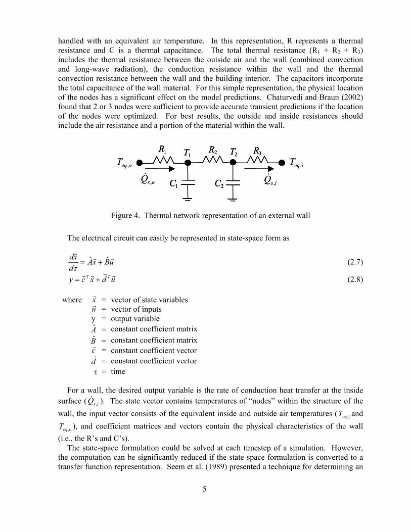
handled with an equivalent air temperature. In this representation, R represents a thermal resistance and C is a thermal capacitance. The total thermal resistance (R1 + R2 + R3) includes the thermal resistance between the outside air and the wall (combined convection and long-wave radiation), the conduction resistance within the wall and the thermal convection resistance between the wall and the building interior. The capacitors incorporate the total capacitance of the wall material. For this simple representation, the physical location of the nodes has a significant effect on the model predictions. Chaturvedi and Braun (2002) found that 2 or 3 nodes were sufficient to provide accurate transient predictions if the location of the nodes were optimized. For best results, the outside and inside resistances should include the air resistance and a portion of the material within the wall.

2C1C

1R 2R 3R1T 2T

osQ ,&

isQ ,&

oeqT , ieqT ,

2C2C1C1C

1R1R 2R2R 3R3R1T1T 2T2T

osQ ,&

isQ ,&

oeqT , ieqT ,

Figure 4. Thermal network representation of an external wall

The electrical circuit can easily be represented in state-space form as

uBxAd

xd rrr

ˆˆ +=τ

(2.7) rrrr udxcy TT += (2.8)

where xr

r = vector of state variables

u = vector of inputs y = output variable A = constant coefficient matrix

Br = constant coefficient matrix c

r = constant coefficient vector

d = constant coefficient vector τ = time

For a wall, the desired output variable is the rate of conduction heat transfer at the inside

surface ( ). The state vector contains temperatures of “nodes” within the structure of the wall, the input vector consists of the equivalent inside and outside air temperatures (T and

), and coefficient matrices and vectors contain the physical characteristics of the wall (i.e., the R’s and C’s).

isQ ,&

ieq,

oeqT ,

The state-space formulation could be solved at each timestep of a simulation. However, the computation can be significantly reduced if the state-space formulation is converted to a transfer function representation. Seem et al. (1989) presented a technique for determining an

5

equivalent transfer function representation from the state-space representation that involves the exact solution to the set of first-order differential equations with the inputs modeled as continuous, piecewise linear functions. This approach is used within VSAT for a one-hour timestep to determine a transfer function equation at the beginning of the simulation. After the transfer function has been developed, then the solution for the output at any time t is of the form

( ) ( )∑∑==

∆− ∆−⋅−⋅=statestate N

kk

N

kkt

Tk ktyeuSty

10ττ

rr (2.9)

where Nstate = number of state variables

kSr

= vector containing transfer function coefficients for the input vector k timesteps prior to the current time t

ek = transfer function coefficient for the zone sensible load for k timesteps prior to the current time t

∆τ = time step (one hour for VSAT)

At the beginning of the simulation, the vectors kSr

for k = 0 to Nstate are determined as

( )[ ] (( ) deRcS

NjdeRRcS

dRcS

statestatestate NNN

statejjjjrrr

rrr)

rrr

+Γ−Γ=

−≤≤+Γ+Γ−Γ=

+Γ=

−

−

211

2211

200

ˆ11for ˆˆ

ˆ

(2.10)

where

( )

−∆Γ

=Γ

−Φ=Γ

−

−

BA

BIA

ˆˆ

ˆˆˆ

112

11

τ

(2.11)

where I is the identity matrix, ∆τ is the simulation time step (one hour for this study), and

( ) ( ) ( )KK +

∆++

∆+

∆+∆+=

=Φ

∆

∆

!

ˆ

!3

ˆ

!2

ˆˆˆ3322

ˆ

ˆ

nAAAAIe

enn

A

A

τττττ

τ

(2.12)

Seem et al. (1989) presented an efficient algorithm for evaluating e in equation 2.12

that is used within VSAT. The matrices used in the determination of r

and the e

τ∆A

jR kS j transfer function coefficients are determined recursively as

6

( )

( )

( )

( )state

NNNNN N

RTreIeRR

RTreIeRR

RTreIeRR

RTreIR

state

statestatestatestate

1121

23212

12101

010

ˆ ˆˆˆ

3

ˆˆˆˆ

2

ˆˆˆˆ

1

ˆˆˆ

−−−−

Φ−=+Φ=

Φ−=+Φ=

Φ−=+Φ=

Φ−==

MM

(2.13)

where Tr() is the trace of the matrix (the sum of the diagonal elements).

The transfer function representation gives the wall conduction at the inside surface for any wall j. The heat transfer to the inside air due to wall j is then

rgjjisji qAQQ ,,,, &&& += (2.14)

2.1.2 Floor Slabs

Slab on grade floors are modeled using a similar formulation as for exterior walls. However, the exterior of the floor is exposed to the ground so that there is no convection, solar radiation, or long-wave radiation. Furthermore, the predominant mechanism for heat loss or gain is heat transfer at the perimeter of the slab. The transfer function of equation 2.9 is used to determine the conduction heat transfer at the inside surface for floors. However, the bottom side of the floor is assumed to be adiabatic (infinite resistance for heat transfer between the outside floor surface and the ground). The primary mode for heat transfer to and from the ambient is through the perimeter of the slab. Perimeter heat transfer is assumed to be quasi-steady state from the ambient to the inside air across a resistance that is based upon the slab perimeter heat loss factor (ASHRAE, 2001). The combined heat transfer to the inside air from the floor is then

)(,, ioprgisi TTPFqAQQ −⋅⋅++= &&& (2.15)

where Fp is the slab perimeter heat loss factor and P is the perimeter of the slab. 2.1.3 Interior Walls

An interior wall differs from an exterior wall in that the inside boundary conditions are experienced on both sides of the wall. The transfer function of equation 2.9 is used to determine the conduction heat transfer at the inside surfaces for interior walls with both boundary conditions given by equation 2.6. Interior walls are assumed to be symmetric with identical boundary conditions, so that the total heat transfer to the air from both surfaces is

( )rgisi qAQQ ,,2 &&& +⋅= (2.16)

7

where A is the surface area for one face and Q is the conduction heat transfer rate for one surface of the wall.

is,&

Interior walls/furnishings are represented with a single node (capacitance) having a total surface area equal to twice the total floor area, a mass of 25 lbm/ft2, and an average specific heat of 0.2 Btu/lbm-F. 2.1.4 Windows

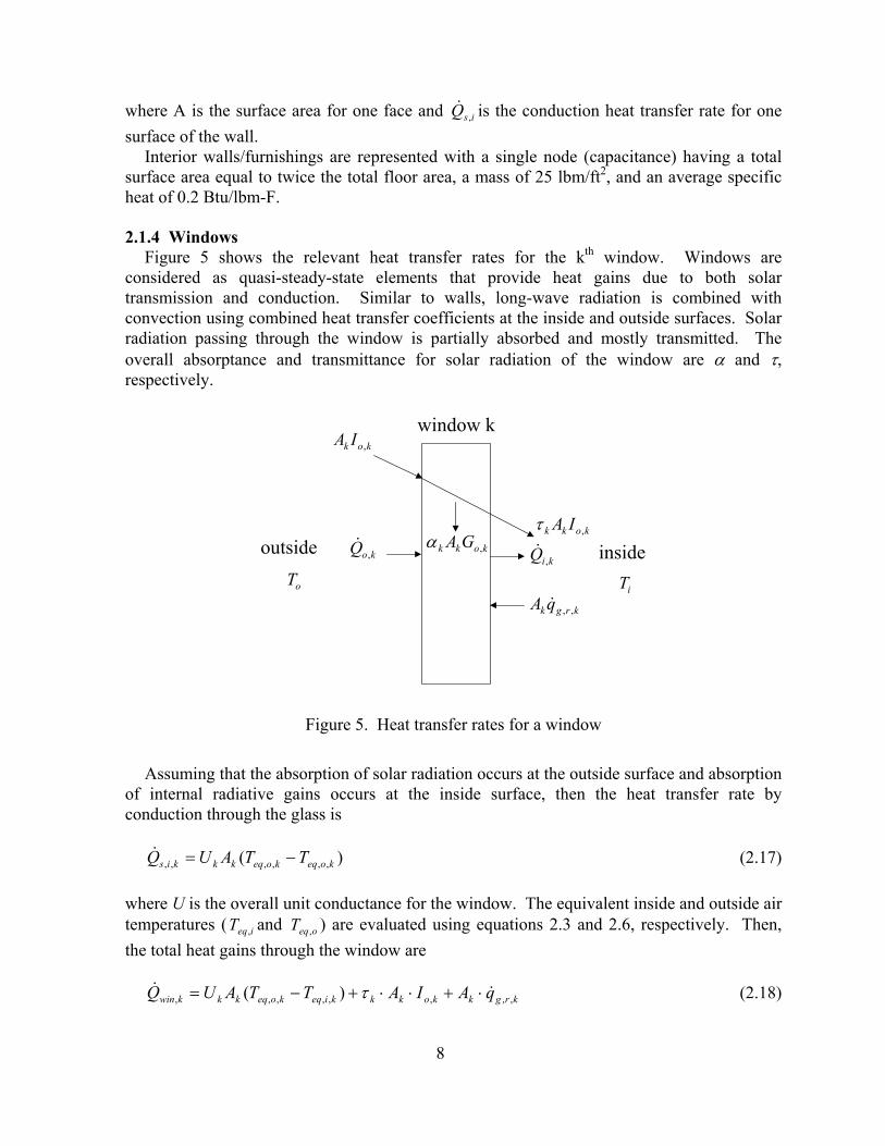
Figure 5 shows the relevant heat transfer rates for the kth window. Windows are considered as quasi-steady-state elements that provide heat gains due to both solar transmission and conduction. Similar to walls, long-wave radiation is combined with convection using combined heat transfer coefficients at the inside and outside surfaces. Solar radiation passing through the window is partially absorbed and mostly transmitted. The overall absorptance and transmittance for solar radiation of the window are α and τ, respectively.

kiQ ,&koQ ,

&

window k

insideoutside

kok IA ,

oTiT

kokk IA ,τkokk GA ,α

krgk qA ,,&

Figure 5. Heat transfer rates for a window

Assuming that the absorption of solar radiation occurs at the outside surface and absorption

of internal radiative gains occurs at the inside surface, then the heat transfer rate by conduction through the glass is

)( ,,,,,, koeqkoeqkkkis TTAUQ −=& (2.17)

where U is the overall unit conductance for the window. The equivalent inside and outside air temperatures (T and ) are evaluated using equations 2.3 and 2.6, respectively. Then, the total heat gains through the window are

ieq, oeqT ,

krgkkokkkieqkoeqkkkwin qAIATTAUQ ,,,,,,,, )( && ⋅+⋅⋅+−= τ (2.18)

8

It is more common to have data for window shading coefficients than for window

transmittances. The shading coefficient accounts for both solar transmission and solar absorption. In this formulation, the total heat gain to the air due to the window is given as

krgkkokkkieqokkkwin qAIASHGCTTAUQ ,,,,,, )( && ⋅+⋅⋅+−= (2.19)

where SHGC is the solar heat gain coefficient defined as

ohUSHGC ατ += (2.20)

where ho is the outside heat transfer coefficient (combined convection and long-wave radiation). Equations 2.18 and 2.19 are equivalent.

The shading coefficient is defined as

refSHGCSHGCSC = (2.21)

where SHGCref is the solar heat gain coefficient for a single pane of double strength glass, which has a value of 0.87. In general, the shading coefficient can account for multiple glazings, different types of glazing materials, and indoor shading devices.

Using the definition of shading coefficient, equation 2.19 can be rewritten as

krgkkokrefkieqokkkwin qAIASHGCSCTTAUQ ,,,,,, )( && ⋅+⋅⋅⋅+−= (2.22) The concept of a shading coefficient was developed for building models where the heat

gains due to solar radiation are added directly to the air. In reality, solar transmission through windows leads to solar absorptance on other interior surfaces, whereas solar absorption in windows leads to increased convection to the air by the window. Although it is not strictly correct, VSAT uses the total solar gains determined with a shading coefficient and distributes them to other internal surfaces. With this approach, the window solar transmission and convection to the air are determined as

kokrefkt IASHGCSCQ ,, ⋅⋅⋅=& (2.23)

krgkkieqokkki qATTAUQ ,,,,, )( && ⋅+−= (2.24)

VSAT assumes constant values for the shading coefficient and overall window unit

conductance. Solar transmission through windows is distributed solely to the floor with a uniform heat flux. 2.1.5 Infiltration

Infiltration is a relatively small effect for commercial buildings and is modeled with a constant flow rate that is based upon a specified volumetric flow rate per unit floor area. The

9

default value is 0.05 cfm/ft2, but can be changed. For a building with 10-foot ceiling height, this infiltration rate corresponds to 0.3 air changes per hour.

The sensible and latent heat gains due to infiltration are determined as

)(infinf, iopms TTCmQ −= && (2.25)

)(infinf, iofgL hmQ ωω −= && (2.26) where Cpm is the moist air specific heat, hfg is the heat of vaporization of water, ωo is the humidity ratio of the outside air, and ωi is the humidity ratio of the inside air. 2.1.7 Internal Gains

Internal gains due to lights, equipment, and people vary according to an occupancy schedule that is specified. The specific values of the heat gains and the proportion of gains from people that influence latent loads vary according to building type (see Prototypical Building Descriptions). For people and lights, 50% of the heat gains are assumed to be radiative and 50% convective. All the gains from equipment (e.g, computers) are assumed to be convective. The radiative internal gains are distributed with an even heat flux to all internal surfaces (including windows).

2.1.8 Zone Loads

At any time, the sensible cooling (+) or heating (-) required to keep the zone temperature at a specified setpoint is determined as

inf,,1

,1

, scg

windows

kki

walls

jjiz QQQQQ &&&&& +++= ∑∑

==

(2.27)

where is the total convective heat gain due to lights, people, and equipment. cgQ ,

&

Separate temperature setpoints are specified for heating and cooling and the temperature can float in between with no required cooling or heating. In order to evaluate whether heating or cooling is required for a given time step, it is necessary to determine the zone temperature where the sensible cooling requirement for the equipment is equal to zero. In the absence of ventilation (unoccupied mode) then equation 2.27 would be solved inversely for the floating inside air temperature with Q set equal to zero. If the calculated zone temperature is less than the heating setpoint, then heating is required and equation 2.27 is evaluated using the heating setpoint. If the calculated zone temperature is greater than the cooling setpoint, then cooling is required and equation 2.27 is evaluated using the cooling setpoint. If the calculated temperature is between the setpoints, then the zone temperature is floating and the zone sensible cooling and heating requirement are zero. The case where the fans operate continuously with a ventilation load (unoccupied mode) is considered in section 4.

z&

When there is a sensible cooling requirement, then the cooling equipment also provides latent cooling and it is necessary to know the latent loads for the zone. In this case, the zone latent gains are the sum of the latent gains due to people and due to infiltration.

10

2.1.9 Solar Radiation Processing

The weather data files used by VSAT contain hourly values of global horizontal radiation and direct normal radiation. The horizontal radiation is used for the roof, but it is necessary to calculate incident radiation on vertical surfaces for external walls. The total incident radiation for vertical surfaces is determined as

HgD

szDNo II

II ργγθ ++−⋅=2

)cos()sin( (2.28)

where IDN is beam radiation that is measured normal to the line of sight to the sun, θz is the zenith angle, γs is the solar azimuth angle, γ is the surface azimuth angle, ID is sky diffuse radiation, ρg is ground reflectance, and IH is total radiation incident upon a horizontal surface. Zenith is the angle between the vertical and the line of site to the sun. Solar azimuth is the angle between the local meridian and the projection of the line of sight to the sun onto the horizontal plane. Zero solar azimuth is facing the equator, west is positive, while east is negative. The zenith and solar azimuth angle are calculated using relationships given in Duffie and Beckman (1980). The surface azimuth is the angle between the local meridian and the projection of the normal to the surface onto the horizontal plane (0 for south facing, -90 for east facing +90 for west facing, and +180 for north facing). The ground reflectance is assumed to have a constant value of 0.2, which is representative of summer conditions. The sky diffuse radiation is calculated from the

)cos( zDNHD III θ−= (2.29)

2.2 Prototypical Building Descriptions Seven different types of buildings are considered in VSAT: small office, school class wing,

retail store, restaurant dining area, school gymnasium, school library, and school auditorium. Descriptions for these buildings were obtained from prototypical building descriptions of commercial building prototypes developed by Lawrence Berkeley National Laboratory (Huang, et al. 1990 & Huang, et al. 1995). These reports served as the primary sources for prototypical building data. However, additional information was obtained from DOE-2 input files used by the researchers for their studies.

Tables 1 - 7 contain information on the geometry, construction materials, and internal gains used in modeling the different buildings. Although not given in these tables, the walls, roofs and floors include inside air and outside air thermal resistances. The window R-value includes the effects of the window construction and inside and outside air resistances. Table 8 lists the properties of all construction materials and the air resistances. The geometry of each of the buildings is assumed to be rectangular with four sides and is specified with the following parameters: 1) floor area, 2) number of stories, 3) aspect ratio, 4) ratio of exterior perimeter to total perimeter, 5) wall height and 6) ratio of glass area to wall area. The aspect ratio is the ratio of the width to the length of the building. However, exterior perimeter and glass areas are assumed to be equally distributed on all sides of the building, giving equal exposure of exterior walls and windows to incident solar radiation. The four exterior walls face north, south, east, and west.

The user can specify occupancy schedules, but default values are based upon the original LBNL study. In the LBNL study, the occupancy was scaled relative to a daily average

11

maximum occupancy density (people per 1000 ft2). In VSAT, the user can specify a peak design occupancy density (people per 1000 ft2) that is used for determining fixed ventilation requirements (no DCV). This same design occupancy density is used as the scaling factor for the hourly occupancy schedules. As a result, the original LBNL occupancy schedules were rescaled using the default peak design occupancy densities.

The heat gains and CO2 generation per person depend upon the type of building (and associated activity). Design internal gains for lights and equipment also depend upon the building and are scaled according to specified average daily minimum and maximum gain fractions. For all of the buildings, the lights and equipment are at their average maximum values whenever the building is occupied and are at their average minimum values at all other times.

Zone thermostat setpoints can be set for both occupied and unoccupied periods. The default occupied setpoints for cooling and heating are 75°F and 70°F, respectively. The default unoccupied setpoints for cooling (setup) and heating (setback) are 85°F and 60°F, respectively. The lights are assumed to come on one hour before people arrive and stay on one hour after they leave. The occupied and unoccupied setpoints follow this same schedule.

12

Table 1. Office Building Characteristics Windows R-value, hr-ft2-F/Btu 1.58 Shading Coefficient 0.75 Area ratio (window/wall) 0.15 Exterior Wall Construction Layers 1” stone

R-5.6 insulation R-0.89 airspace 5/8” gypsum

Roof Construction Layers Built-up roof (3/8”)

4” lightweight concrete R-12.6 insulation R-0.92 airspace ½” acoustic tile

Floor Layers 6” heavyweight

concrete Carpet and pad

Slab perimeter loss factor, Btu/h-ft-F 0.5 General Floor area, ft2 6600 Wall height, ft 11 Internal mass, lb/ft2 25 Number of stories 1 Aspect Ratio 0.67 Ratio of exterior perimeter to floor perimeter 1.0 Design equipment gains, W/ft2 0.5 Design light gains, W/ft2 1.7 Ave. daily min. lights/equip. gain fraction 0.2 Ave. daily max. lights/equip. gain fraction 0.9 Sensible people gains, Btu/hr-person 250 Latent people gains, Btu/hr-person 250 CO2 people generation, L/min-person 0.33 Design occupancy for vent., people/1000 ft2 7 Design ventilation, cfm/person 20 Average weekday peak occucpancy, ft2/person

470

Default average weekday occupancy schedule * Values given relative to average peak

Hours 1-7 8 9 10-16 17 18-24

Values 0.0 0.33 0.66 1.0 0.5 0.0

Default average weekend occupancy schedule * Values given relative to average peak

Hours 1-8 9 10-12 12-13 13-24

Values 0.0 0.15 0.2 0.15 0.0

Monthly occupancy scaling * relative to daily occupancy schedule

Month 1-12

Value 1.0

13

Table 2. Restaurant Dining Area Characteristics Windows R-value, hr-ft2-F/Btu 1.53 Shading Coefficient 0.8 Area ratio (window/wall) 0.15 Exterior Wall Construction Layers 3” face brick

½” plywood R-4.9 insulation 5/8” gypsum


¾” plywood R-13.2 insulation R-0.92 airspace ½” acoustic tile

Floor Layers 4” heavyweight concrete

Carpet and pad Slab perimeter loss factor, Btu/h-ft-F 0.5 General Floor area, ft2 4200 Wall height, ft 10 Internal mass, lb/ft2 25 Number of stories 1 Aspect Ratio 1.0 Ratio of exterior perimeter to floor perimeter 0.75 Design equipment gains, W/ft2 0.0 Design light gains, W/ft2 2.0 Ave. daily min. lights/equip. gain fraction 0.2 Ave. daily max. lights/equip. gain fraction 1.0 Sensible people gains, Btu/hr-person 250 Latent people gains, Btu/hr-person 275 CO2 people generation, L/min-person 0.35 Design occupancy for vent., people/1000 ft2 30 Design ventilation, cfm/person 20 Average weekday peak occucpancy, ft2/person

50


Hours 1-6 7-12 13-24

Values 0.0 0.2,0.3,0.1,0.05,0.2,0.5 0.5,0.4,0.2,0.05,0.1,0.4, 0.6,0.5,0.4,0.2,0.1,0.0


Hours 1-6 7-12 13-24

Values 0.0 0.3,0.4,0.5,0.2,0.2,0.3 0.5,0.5,0.5,0.35,0.25, 0.5,0.8,0.8,0.7,0.4,0.2, 0.0


Month 1-5 6-8 9-12

Value 1.0 0.5 1.0

14

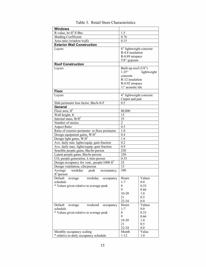
Table 3. Retail Store Characteristics Windows R-value, hr-ft2-F/Btu 1.5 Shading Coefficient 0.76 Area ratio (window/wall) 0.15 Exterior Wall Construction Layers 8” lightweight concrete

R-4.8 insulation R-0.89 airspace 5/8” gypsum


1.25” lightweight concrete R-12 insulation R-0.92 airspace ½” acoustic tile

Floor Layers 4” lightweight concrete

Carpet and pad Slab perimeter loss factor, Btu/h-ft-F 0.5 General Floor area, ft2 80,000 Wall height, ft 15 Internal mass, lb/ft2 25 Number of stories 2 Aspect Ratio 0.5 Ratio of exterior perimeter to floor perimeter 1.0 Design equipment gains, W/ft2 0.4 Design light gains, W/ft2 1.6 Ave. daily min. lights/equip. gain fraction 0.2 Ave. daily max. lights/equip. gain fraction 0.9 Sensible people gains, Btu/hr-person 250 Latent people gains, Btu/hr-person 250 CO2 people generation, L/min-person 0.33 Design occupancy for vent., people/1000 ft2 25 Design ventilation, cfm/person 15 Average weekday peak occucpancy, ft2/person

390


Hours 1-7 8 9 10-20 21 22-24

Values 0.0 0.33 0.66 1.0 0.5 0.0


Hours 1-7 8 9 10-20 21 22-24

Values 0.0 0.33 0.66 1.0 0.5 0.0


Month 1-12

Value 1.0

15

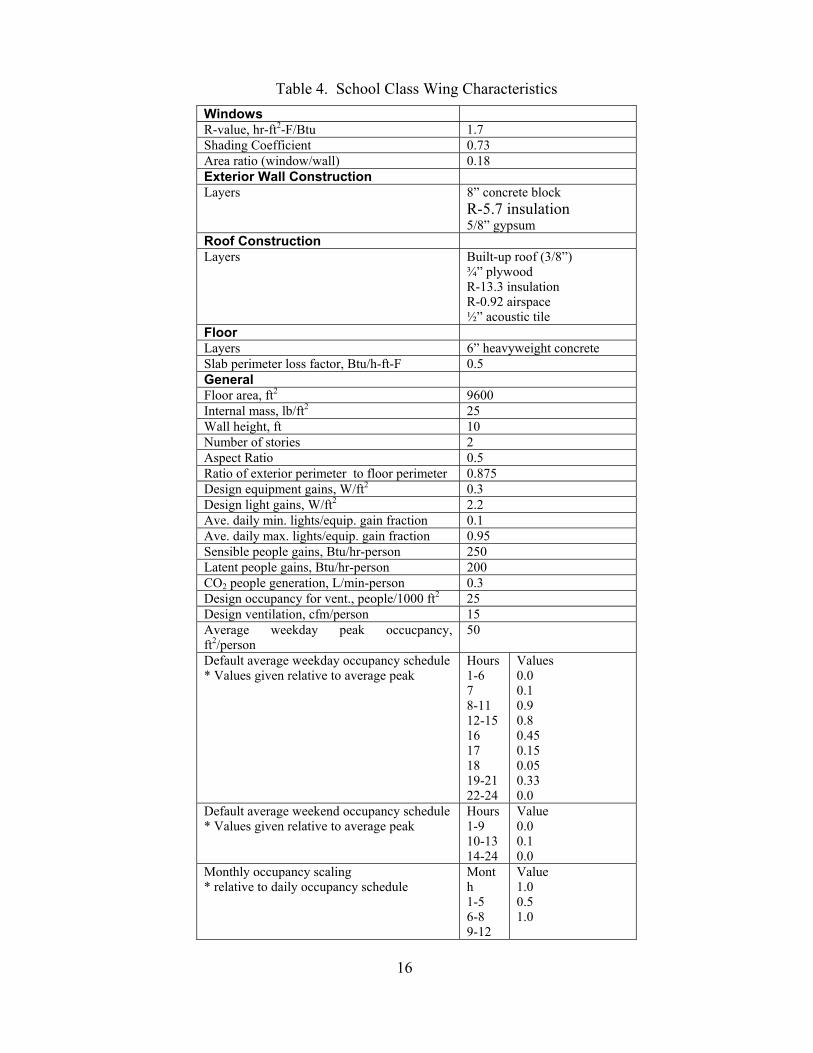
Table 4. School Class Wing Characteristics Windows R-value, hr-ft2-F/Btu 1.7 Shading Coefficient 0.73 Area ratio (window/wall) 0.18 Exterior Wall Construction Layers 8” concrete block

R-5.7 insulation 5/8” gypsum



Floor Layers 6” heavyweight concrete Slab perimeter loss factor, Btu/h-ft-F 0.5 General Floor area, ft2 9600 Internal mass, lb/ft2 25 Wall height, ft 10 Number of stories 2 Aspect Ratio 0.5 Ratio of exterior perimeter to floor perimeter 0.875 Design equipment gains, W/ft2 0.3 Design light gains, W/ft2 2.2 Ave. daily min. lights/equip. gain fraction 0.1 Ave. daily max. lights/equip. gain fraction 0.95 Sensible people gains, Btu/hr-person 250 Latent people gains, Btu/hr-person 200 CO2 people generation, L/min-person 0.3 Design occupancy for vent., people/1000 ft2 25 Design ventilation, cfm/person 15 Average weekday peak occucpancy, ft2/person

50


Hours 1-6 7 8-11 12-15 16 17 18 19-21 22-24

Values 0.0 0.1 0.9 0.8 0.45 0.15 0.05 0.33 0.0


Hours 1-9 10-13 14-24

Value 0.0 0.1 0.0


Month 1-5 6-8 9-12

Value 1.0 0.5 1.0

16

Table 5. School Gymnasium Characteristics Windows R-value, hr-ft2-F/Btu 1.7 Shading Coefficient 0.73 Area ratio (window/wall) 0.18 Exterior Wall Construction Layers 8” concrete block





180


Hours 1-7 8-15 16-24

Value 0.0 1.0 0.0


Hours 1-24

Value 0.0


Month 1-5 6-8 9-12

Value 1.0 0.1 1.0

17

Table 6. School Library Characteristics Windows R-value, hr-ft2-F/Btu 1.7 Shading Coefficient 0.73 Area ratio (window/wall) 0.18 Exterior Wall Construction Layers 8” concrete block





100


Hours 1-6 7 8-11 12-15 16 17 18 19-21 22-24

Value 0.0 0.1 0.9 0.8 0.45 0.15 0.05 0.33 0.0


Hours 1-9 10-13 14-24

Value 0.0 0.1 0.0


Month 1-5 6-8 9-12

Value 1.0 0.5 1.0

18

Table 7. School Auditorium Characteristics Windows R-value, hr-ft2-F/Btu 1.7 Shading Coefficient 0.73 Area ratio (window/wall) 0.18 Exterior Wall Construction Layers 8” concrete block





100


Hours 1-9 10-11 12 13-14 15-24

Values 0.0 0.75 0.2 0.75 0.0


Hours 1-24

Value 0.0


Month 1-5 6-8 9-12

Value 1.0 0.1 1.0

19

Table 8. Construction Material Properties

Conductivity (Btu/h*ft*F)

Density (lb/ft3)

Specific Heat (Btu/lb*F)

stone 1.0416 140 0.20light concrete 0.2083 80 0.20heavy concrete 1.0417 140 0.20built-up roof 0.0939 70 0.35face brick 0.7576 130 0.22acoustic tile 0.033 18 0.32gypsum 0.0926 50 0.20

Resistance (h*ft2*F/Btu)

3/4" plywood 0.937031/2" plywood 0.62469carpet and pad 2.08inside air 0.67outside air 0.33

2.3 Model Validation

The prototypical buildings were chosen to give representative building loads in order to determine if particular building types will benefit more or less from the ventilation strategies under examination. Absolute model predictions are not the goal but rather the impact of ventilation strategies on savings compared to a baseline. Even so, it is very important that the building load predictions have representative dynamics and absolute load levels. In order to validate predictions of VSAT, results have been compared with predictions of the TYPE 56 building model within TRNSYS (2000). This model has been validated with detailed measurements and through comparison with other accepted building load calculation programs.

The TYPE 56 is a very detailed model that is built up from individual descriptions of wall layers, windows, internal gains, schedules, etc. The user enters all pertinent information into a “front-end” program called PRE-BID. This program assimilates all the information into four different files that are used by the TYPE 56 component for generating the specific building loads and ultimately the total building load.

Two building prototypes were chosen as case studies to validate the building loads portion of VSAT. Identical construction properties, schedules, internal gains and weather data for each case study were entered into the TYPE 56 and VSAT models for comparison.

2.3.1 TYPE 56 and VSAT Building Model Assumptions The TYPE 56 building type predicts the thermal behavior of a building having multiple

zones. To determine zone heating and cooling requirements, an “energy rate” method is employed. The user specifies the zone setpoints for heating and cooling with any added setup or setback control schedules. If the floating zone temperature is less than the heating setpoint,

20

then heating is required or if the calculated zone temperature is greater than the cooling setpoint, then cooling is required. Otherwise, the zone temperature is floating and the zone sensible cooling and heating requirement are zero. Unlimited equipment capacity was assumed in the TYPE 56 for purposes of validating the building model in the VSAT.

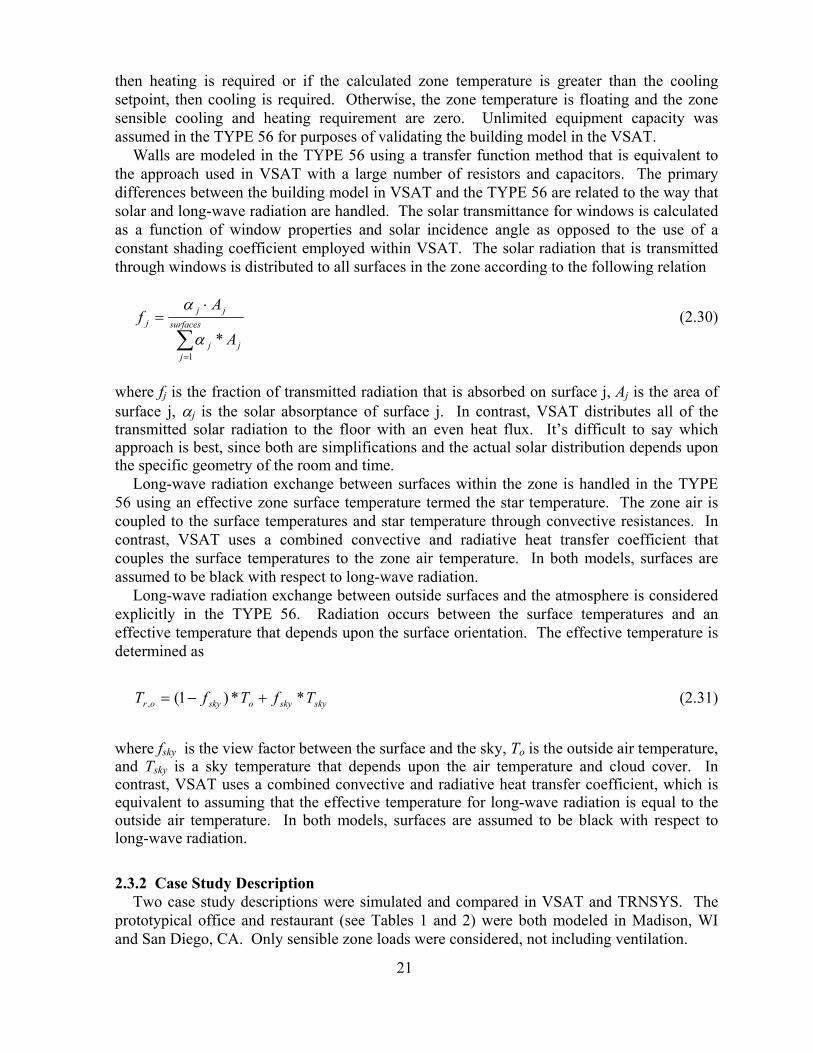
Walls are modeled in the TYPE 56 using a transfer function method that is equivalent to the approach used in VSAT with a large number of resistors and capacitors. The primary differences between the building model in VSAT and the TYPE 56 are related to the way that solar and long-wave radiation are handled. The solar transmittance for windows is calculated as a function of window properties and solar incidence angle as opposed to the use of a constant shading coefficient employed within VSAT. The solar radiation that is transmitted through windows is distributed to all surfaces in the zone according to the following relation

∑=

⋅= surfaces

jjj

jjj

A

Af

1*α

α (2.30)

where fj is the fraction of transmitted radiation that is absorbed on surface j, Aj is the area of surface j, αj is the solar absorptance of surface j. In contrast, VSAT distributes all of the transmitted solar radiation to the floor with an even heat flux. It’s difficult to say which approach is best, since both are simplifications and the actual solar distribution depends upon the specific geometry of the room and time.

Long-wave radiation exchange between surfaces within the zone is handled in the TYPE 56 using an effective zone surface temperature termed the star temperature. The zone air is coupled to the surface temperatures and star temperature through convective resistances. In contrast, VSAT uses a combined convective and radiative heat transfer coefficient that couples the surface temperatures to the zone air temperature. In both models, surfaces are assumed to be black with respect to long-wave radiation.

Long-wave radiation exchange between outside surfaces and the atmosphere is considered explicitly in the TYPE 56. Radiation occurs between the surface temperatures and an effective temperature that depends upon the surface orientation. The effective temperature is determined as

skyskyoskyor TfTfT **)1(, +−= (2.31)

where fsky is the view factor between the surface and the sky, To is the outside air temperature, and Tsky is a sky temperature that depends upon the air temperature and cloud cover. In contrast, VSAT uses a combined convective and radiative heat transfer coefficient, which is equivalent to assuming that the effective temperature for long-wave radiation is equal to the outside air temperature. In both models, surfaces are assumed to be black with respect to long-wave radiation.

2.3.2 Case Study Description Two case study descriptions were simulated and compared in VSAT and TRNSYS. The

prototypical office and restaurant (see Tables 1 and 2) were both modeled in Madison, WI and San Diego, CA. Only sensible zone loads were considered, not including ventilation.

21

In VSAT, combined convective and radiation coefficients were utilized for the inside and

outside air of 1.5 Btu/hr-ft2-F and 3.0 Btu/hr-ft2-F, respectively. Since long-wave radiation is handled explicitly in the TYPE 56, convective heat transfer coefficients need to be specified for the inside and outside air. Convective heat transfer coefficients that result in approximately the combined coefficients used in VSAT were found to be 1.25 Btu/hr-ft2-F and 2.75 Btu/hr-ft2-F and were used within the TYPE 56.

The TYPE 56 estimates U-Values for windows based upon the glass properties. For a single pane glass, the U-Value is about 1.0 Btu/hr-ft2-F. In order to realize the specified overall R-values for the windows used in VSAT, the outside and inside convective heat transfer coefficients were set to 2.3 Btu/hr-ft2-F and 6.8 Btu/hr-ft2-F for windows within the TYPE 56.

In order to distribute transmitted solar radiation to the floor only, the solar absorptances of all inside walls were set to zero in the TYPE 56 and the floor solar absorptance was set equal to unity. Finally, the sky temperature used by the TYPE 56 was set equal to the ambient temperature.

2.3.3 Results for Constant Temperature Setpoints As a first step, cooling and heating loads were evaluated for a constant temperature

setpoint of 70°F (21.11°C). This eliminates any transients due to return from night setup and setback. Figure 6 shows hourly heating load comparisons for the office and restaurant over two days in January. VSAT predicts the correct transients and peak load. The relative differences are largest when the loads are smallest at night. Similar results are shown for two days of cooling load predictions in Figure 7.

0

6000

12000

18000

24000

30000

1 6 11 16 21 26 31 36 41 46

Hour

Sens

ible

Hea

ting

Load

(W)

TRNSYSVSAT

Office

0

6000

12000

18000

24000

30000

1 6 11 16 21 26 31 36 41 46

Hour

Sens

ible

Hea

ting

Load

(W)

TRNSYSVSATTRNSYSVSAT

Office

0

6000

12000

18000

1 6 11 16 21 26 31 36 41 46

Hour

Sens

ible

Hea

ting

Load

(W)

TRNSYSVSAT

Restaurant

0

6000

12000

18000

1 6 11 16 21 26 31 36 41 46

Hour

Sens

ible

Hea

ting

Load

(W)


Restaurant

Figure 6. Hourly zone heating loads for constant setpoints (Jan. 9 – 10, Madison, WI)

22

0

6000

12000

18000

24000

1 6 11 16 21 26 31 36 41 46Hour

Sens

ible

Coo

ling

Load

(W)

TRNSYSVSAT

Office

0

6000

12000

18000

24000

1 6 11 16 21 26 31 36 41 46Hour

Sens

ible

Coo

ling

Load

(W)


Office

0

6000

12000

18000

24000

1 6 11 16 21 26 31 36 41 46Hour

Sens

ible

Coo

ling

Load

(W)

TRNSYSVSAT

Restaurant

0

6000

12000

18000

24000

1 6 11 16 21 26 31 36 41 46Hour

Sens

ible

Coo

ling

Load

(W)


Restaurant

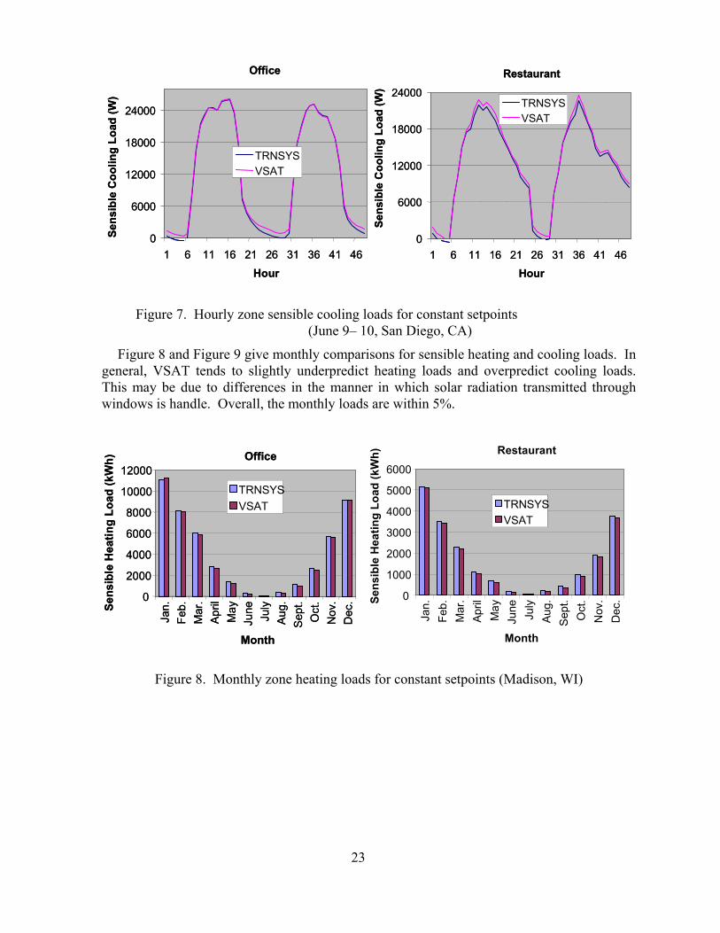
Figure 7. Hourly zone sensible cooling loads for constant setpoints (June 9– 10, San Diego, CA)

Figure 8 and Figure 9 give monthly comparisons for sensible heating and cooling loads. In general, VSAT tends to slightly underpredict heating loads and overpredict cooling loads. This may be due to differences in the manner in which solar radiation transmitted through windows is handle. Overall, the monthly loads are within 5%.

0

2000

4000

6000

8000

10000

12000

Jan.

Feb.

Mar

.Ap

rilM

ayJu

ne July

Aug.

Sept

.O

ct.

Nov

.D

ec.

Month

Sens

ible

Hea

ting

Load

(kW

h)

TRNSYSVSAT

Office

0

2000

4000

6000

8000

10000

12000

Jan.

Feb.

Mar

.Ap

rilM

ayJu

ne July

Aug.

Sept

.O

ct.

Nov

.D

ec.

Month

Sens

ible

Hea

ting

Load

(kW

h)


Office

0

1000

2000

3000

4000

5000

6000

Jan.

Feb.

Mar

.Ap

rilM

ayJu

ne July

Aug.

Sept

.O

ct.

Nov

.D

ec.

Month

Sens

ible

Hea

ting

Load

(kW

h)


Restaurant

Figure 8. Monthly zone heating loads for constant setpoints (Madison, WI)

23

0

2000

4000

6000

8000

10000

12000

Jan.

Feb.

Mar

.

April

May

June July

Aug.

Sept

.

Oct

.

Nov

.

Dec

.

Month

Sens

ible

Coo

ling

Load

(kW

h)

TRNSYSVSAT

Office

0

2000

4000

6000

8000

10000

12000

Jan.

Feb.

Mar

.

April

May

June July

Aug.

Sept

.

Oct

.

Nov

.

Dec

.

Month

Sens

ible

Coo

ling

Load

(kW

h)


Office

0

2000

4000

6000

8000

10000

12000

Jan.

Feb.

Mar

.Ap

rilM

ayJu

ne July

Aug.

Sept

.O

ct.

Nov

.D

ec.

Month

Sens

ible

Coo

ling

Load

(kW

h)


Restaurant

Figure 9. Monthly zone sensible cooling loads for constant setpoints (San Diego, CA)

2.3.4 Results for Night Setback/ Setup Control

The use of a night setback/setup thermostat results in significant dynamics at the start of the occupied period that are not encountered with constant setpoints. Results were generated using both the TYPE 56 and VSAT with night setup for cooling and night setback for heating. For cooling, the occupied period setpoint temperature was 75°F (23.89°C) and the unoccupied setpoint (night setup) temperature was 85°F (29.44°C). For heating, the occupied setpoint was 70°F (21.11°C) and the unoccupied setpoint (night setback) temperature was 60°F (15.56°C). Figure 10 shows sample hourly heat requirements and hourly average zone temperatures for the office in Madison. For both models, there is a large “spike” in the heating requirements when the setpoint returns to the occupied value at 7 am (one hour prior to occupancy). However, the spike is much larger for VSAT than for TRNSYS. This difference is due to differences in the way that zone temperature setpoint adjustsments are handled in the two models. VSAT models a true step change in the setpoint at 7 am, whereas TRNSYS assumes a linear variation in setpoint over the course of the hour from 7 am to 8 am. This difference is apparent in the zone temperature results in Figure 10. Similar results were obtained for the restaurant.

Figure 11 shows similar results for cooling in Madison. Once again, VSAT exaggerates the effect of return from night setup on the cooling loads because it assumes a pure step change in the temperature. Figure 11 also shows that both TRNSYS and VSAT predict similar floating temperatures during the setup (nighttime) period.

Figure 12 shows monthly heating and sensible cooling loads for the office in Madison with night setback/setup control. VSAT tends to overpredict the integrated loads by about 5%. This is partly due to the overprediction of loads at the onset of the return from night setback/setup.

24

0

20000

40000

60000

80000

100000

1 6 11 16 21 26 31 36 41 46Hour

Sens

ible

Loa

d (W

) TRNSYSEstimatorTRNSYSVSAT

0

20000

40000

60000

80000

100000

1 6 11 16 21 26 31 36 41 46Hour

Sens

ible

Loa

d (W

) TRNSYSEstimatorTRNSYSVSATTRNSYSEstimatorTRNSYSVSAT

1516171819202122

1 6 11 16 21 26 31 36 41 46

Hour

Zone

Tem

p. (C

)

TRNSYSEstimatorTRNSYSVSAT

1516171819202122

1 6 11 16 21 26 31 36 41 46

Hour

Zone

Tem

p. (C

)

TRNSYSEstimatorTRNSYSVSATTRNSYSEstimatorTRNSYSVSAT

Figure 10. Hourly zone heating loads for the office with night setback

(Jan. 9 – 10, Madison, WI)

0

20000

40000

60000

80000

1 6 11 16 21 26 31 36 41 46Hour

Sens

ible

Loa

d (W

) TRNSYSVSATTRNSYSVSAT

23

24

25

26

27

28

29

1 6 11 16 21 26 31 36 41 46Hour

Zone

Tem

p. (C

)

TRNSYSVSAT

23

24

25

26

27

28

29

1 6 11 16 21 26 31 36 41 46Hour

Zone

Tem

p. (C

)


Figure 11. Hourly zone cooling loads for the office with night setup (June 9 – 10, Madison, WI)

0

2000

4000

6000

8000

10000

Jan.

Feb.

Mar

.A

pril

May

June

July

Aug

.Se

pt.

Oct

.N

ov.

Dec

.

Month

Sens

ible

Loa

d (k

Wh)

TRNSYSVSAT

Heating Loads for Office

0

2000

4000

6000

8000

10000

Jan.

Feb.

Mar

.A

pril

May

June

July

Aug

.Se

pt.

Oct

.N

ov.

Dec

.

Month

Sens

ible

Loa

d (k

Wh)


Heating Loads for Office

0

2000

4000

6000

8000

10000

Jan.

Feb.

Mar

.A

pril

May

June

July

Aug

.Se

pt.

Oct

.N

ov.

Dec

.

Month

Sens

ible

Loa

d (k

Wh)

TRNSYSVSAT

Cooling Loads for Office

0

2000

4000

6000

8000

10000

Jan.

Feb.

Mar

.A

pril

May

June

July

Aug

.Se

pt.

Oct

.N

ov.

Dec

.

Month

Sens

ible

Loa

d (k

Wh)


Cooling Loads for Office

Figure 12. Monthly zone heating and sensible cooling loads for the office with night setup/setup (Madison, WI)

25

2.3.5 Conclusions The TYPE 56 building component in TRNSYS is more detailed and accurate in predicting

building loads than VSAT. However, for the purposes of comparing different ventilation techniques, this level of detail is not required. Except for return from night setback or setup, VSAT predicts very reasonable transients and overall load levels. Furthermore, VSAT is computationally much more efficient than the TYPE 56, which will facilitate large parametric studies involving many locations and system parameters. The issue of large peak loads at return from night setback or setup will be investigated and VSAT will be modified to predict more reasonable load requirements.

26

SECTION 3: HEATING AND COOLING EQUIPMENT MODELS

The primary cooling and heating are provided by unitary equipment incorporating a vapor compression air conditioner, a gas or electric heater, and a supply fan. In addition, rotary air-to-air enthalpy exchangers or heat pump heat recovery units can be used to reduce ventilation loads for the primary equipment. Figure 13 depicts a rooftop unit in combination with a heat pump heat recovery unit operating in cooling mode. Ventilation air is cooled and dehumidified by the heat recovery unit prior to mixing with return air from the zone. The mixed air is further cooled and dehumidified (when necessary) by the primary evaporator of the rooftop unit. Heat is rejected to the building exhaust air from the condenser of the recovery unit. The heat pump contains an exhaust fan. In addition, an optional supply fan is used if necessary to provide the proper ventilation air.

In heating mode, refrigerant flow within the heat pump is changed so that the exhaust air stream is cooled (the condenser becomes an evaporator) and heat is rejected to the ventilation air (the evaporator becomes a condenser). The preheated air is then mixed with return air. Although not shown in Figure 13, a gas or electric heater is located after the evaporator to provide additional heating of the supply air when necessary.

Figure 13. Rooftop air conditioner with heat pump heat recovery unit (cooling mode)

An alternative to heat pump heat recovery is an enthalpy exchanger. Figure 14 depicts a

rotary air-to-air enthalpy exchanger considered in VSAT. The device consists of a revolving cylinder filled with an air-permeable medium having a large internal surface area that incorporates a desiccant material. Adjacent supply and exhaust air streams each flow through the exchanger in a counter-flow direction. Sensible heat is transferred as the wheel acquires heat from the hot air stream and releases it to the cold air stream. Moisture is adsorbed from the high humidity air stream to the desiccant material and desorbed into the low humidity air stream. In cooling mode, warm and moist ventilation air is cooled and dehumidified and exhaust air is warmed and humidified. In heating mode, cool and dry air is heated and humidified and exhaust air is cooled and dehumidified.

27

Figure 14. Rotary air-to-air enthalpy exchanger

This section describes the models used for the primary cooling, heating, and heat recovery

equipment. Different efficiency equipment can be specified, since this may affect the economics of alternative ventilation strategies. Control strategies for this equipment, along with the description of ventilation control strategies are given in Section 4.

3.1 Vapor Compression System Modeling

Both the primary air conditioning and heat pump heat recovery units utilize a basic vapor compression cycle consisting of a compressor, evaporator coil, expansion valve and condenser coil. Both of these devices are modeled using an approach similar to that incorporated in ASHRAE’s HVAC Toolkit (Brandemuehl et al., 1993). The model for the primary air conditioner utilizes prototypical performance characteristics, which are scaled according to the capacity requirements and efficiency at design conditions. The characteristics of the heat pump heat recovery unit are based upon measurements obtained from the manufacturer and from tests conducted at the Herrick Labs, which are also scaled for different applications.

3.1.1 Mathematical Description

Steady-State Capacity and COP The total capacity (cooling or heating), , and coefficient of performance, COP, are

calculated by applying correction factors to values specified at rating conditions. The correction factors include the effects of air temperature entering the condenser (T

capQ&

c,i), evaporator entering wet bulb temperature (Te,wb,i) or dry bulb temperature (Te,i) and air flow rate ( ). For the case where moisture is removed from the air flowing over the evaporator, the capacity and COP are calculated using the following relations

m&

)/(),( ,,,,,, ratmcapiciwbetcapratcapcap mmfTTfQQ &&&& ⋅⋅= (3.1)

)/(),(11,,,,, ratmCOPiciwbetCOP

ratcap

mmfTTfCOPCOP

&&⋅⋅= (3.2)

28

where and COPcapQ& cap are the capacity and COP for the unit in steady state with the current

operating conditions, Q and COPratcap,& rat are the capacity and COP at specified rating

conditions, is the capacity correction factor based on temperature, is the capacity correction factor based on air mass flowrate, f

tcapf , mcapf ,

COP,t is the COP correction factor based on temperature, and fCOP,m is the COP correction factor based on air mass flowrate. The COP is defined as the ratio of the cooling or heating capacity to the power input. For the primary cooling equipment, the power includes both the compressor and condenser fan, but not the evaporator fan. For the heat pump heat recovery unit, the power includes only the compressor. For either type of equipment, the capacity (cooling or heating) does not include the effect of the supply air fan.

For the primary cooling equipment, the inlet wet bulb temperature to the evaporator is associated with the mixed air condition (mixture of outside and return air) and the inlet condenser temperature is the dry bulb ambient temperature (Ta). The air mass flow rate used within the correlations is the flow rate over the evaporator coil. The air flow rate for the condenser is assumed to be the value at the rating condition.

For the heat pump heat recovery unit, the air flow rate used within the correlations is the ventilation flow rate, which is assumed to be equal for the evaporator and condenser (ventilation and exhaust streams considered to have equal flow rates). For the heat pump recovery unit operating in a cooling mode, the inlet wet bulb to the evaporator is the ambient wet bulb temperature (Twb) and the inlet condenser temperature is the return air temperature from the zone (Tz). During heating mode for the heat pump heat recovery unit, the inlet condenser air temperature is the ambient dry bulb temperature and the inlet condition to the evaporator is the state of air returning from the zone. Since the room air is relatively cool and dry, moisture is not generally condensed as the exhaust air flows over the heat pump evaporator. Therefore, the return air dry bulb temperature (Tz) is used in place of the wet bulb temperature for this case.

The correction factors are based upon correlations of the following form.

iciwbeiciciwbeiwbeiciwbetcap TTfTeTdTcTbaTTf ,,,12,1,1

2,,1,,11,,,, ),( ⋅⋅+⋅+⋅+⋅+⋅+= (3.3)

iciwbeiciciwbeiwbeiciwbetCOP TTfTeTdTcTbaTTf ,,,2

2,2,2

2,,2,,22,,,, ),( ⋅⋅+⋅+⋅+⋅+⋅+= (3.4)

( ) ( ) ( )( )( )ratratratratmcap mmdcmmbmmammf &&&&&&&& 3333, )/( +⋅+⋅+= (3.5)

( ) ( ) ( )( )( )ratratratratmCOP mmdcmmbmmammf &&&&&&&& 4444, )/( +⋅+⋅+= (3.6)

Different coefficients are used in equations 3.3 – 3.6 for three different cases: 1) primary

cooling unit, 2) heat pump heat recovery operating in a cooling mode, and 3) heat pump heat recovery operating in heating mode. For the primary cooling, the coefficients are from the DOE 2.1E building simulation program. For the heat pump heat recovery unit, the coefficients were determined using performance data as described in a later section.

For cooling, the evaporator inlet air is not always humid enough to result in moisture condensation. In this case, unit performance depends upon inlet evaporator dry bulb rather than wet bulb temperature. However, the correlations developed in terms of wet bulb should

29

provide accurate predictions as long as the correct inlet dry bulb is used and the inlet humidity is set to a value where condensation just begins. This point represents the end of the range where the correlations apply (i.e., the correlation should apply at the point dehumidification begins to occur). Performance is independent of humidity for lower values. Therefore, if the moisture condensation is found not to occur (see section on sensible heat ratio), then the inlet humidity ratio is adjusted until the point where moisture condensation just beings (sensible heat ratio of one). The air inlet wet bulb temperature associated with the actual dry bulb temperature and this fictitious humidity is then used as the evaporator inlet condition for the capacity and COP correlations.

Sensible Heat Ratio The model for cooling capacity allows determination of the leaving enthalpy using an

energy balance, but not the leaving temperature or humidity. A model for moisture removal is utilized that incorporates the concept of a bypass factor (BF). The bypass factor approach considers two different air streams flowing across the evaporator. One air stream is in close proximity to the coil surface and exits the evaporator as saturated air at the effective temperature of the coil surface and the other air stream is away from the coil and assumed to remain at the entering air condition. Since the air close to the coil is allowed to come into equilibrium with the effective surface temperature at a saturated condition, then the effective surface temperature must be the dewpoint of inlet air. As a result, it is termed the apparatus dewpoint temperature, Tadp.

Mass and energy balances on both air streams give the following

bypapp mmm &&& += (3.7)

iebypadpappoe mmm ,, ωωω &&& += (3.8)

iebypadpappoe hmhmhm ,, &&& += (3.9) where is the total air mass flow rate, m is the air mass flow rate near the coil, is the air mass flow rate away from the coil (bypass), h

m& app& bypm&

e,i and he,o are the evaporator inlet and outlet air enthalpy, and ωe,i and ωe,o are the evaporator inlet and outlet humidity ratio.

The bypass factor is defined as the ratio of the bypass flow to the total flow. With this definition and equations 3.7 – 3.9, the bypass factor can be related to the operating conditions according to

adpie

adpoe

adpie

adpoebyp

hhhh

mm

BFωωωω

−

−=

−

−==

,

,

,

,

&

& (3.10)

For a given bypass factor (BF), equation 3.10 indicates that on a psychrometric chart the outlet air state (heo,ωeo) is on a straight line that connects the inlet state with the apparatus dewpoint. This is depicted in Figure 15. The larger the bypass factor the closer the outlet state is to the inlet state.

30

Saturation Line

he,o

he,i

hadp ωe,o

ωe,i

ωadp

Tadp

Saturation Line

he,o

he,i

hadp

Te,iTe,iTe,iTe,iTe,oTe,oTe,oTe,o

ωe,o

ωe,i

ωadp

Tadp

Figure 15. Psychrometric depiction of evaporator air process

The bypass factor can be determined from the heat transfer characteristics of a specific

evaporator coil. The bypass factor is estimated from

NTUeBF −= (3.11)

( )rated

rated

pm mmNTU

CmUANTU

&&&≈

⋅= (3.12)

and where NTU is the number of transfer units, UA is the air-side conductance of the evaporator coil, Cpm is the specific heat of moist air, and NTUrated is the value of NTU at the rated flow rate. The right-hand form of equation 3.12 employs the assumption that the conductance does not change with air flow rate. NTUrated can be determined from rated performance since the bypass factor can be determined from entering and leaving conditions. Then, the bypass factor is estimated as a function of air flow using equations 3.11 and 3.12.

The outlet air enthalpy for the evaporator operating at steady state is first determined using an energy balance with the known entering enthalpy and the cooling capacity determined as described in the previous section. For a given bypass factor and inlet and outlet enthalpy, the saturated air enthalpy corresponding to the apparatus dewpoint is determined from equation 3.10 as

BFhh

hh oeieieadp −

−−=

1,,

, (3.13)

The apparatus dewpoint temperature and saturated humidity ratio are determined using

psychrometric relationships for a relative humidity of 100% and an air enthalpy of hadp. Then, the outlet air humidity ratio is determined from equation 3.10 as

31

adpieoe BFBF ωωω ⋅−+⋅= )1(,, (3.14)

Since the outlet state lies on the locus of point connecting the inlet and apparatus dewpoint conditions (see Figure 15), the sensible heat ratio (SHR) can be determined as

adpie

adpadpie

hhhTh

SHR−

−=

,

, ),( ω (3.15)

where SHR is the ratio of the sensible cooling capacity to the total cooling capacity.

If the calculated value of SHR is greater then unity, then moisture condensation does not occur and SHR is unity. In this case, the inlet humidity ratio is adjusted until the point where SHR = 1. The air inlet wet bulb temperature associated with the actual dry bulb temperature and this fictitious humidity is then used as the evaporator inlet condition for the capacity and COP correlations given in the previous section.

Compressor Power Consumption

When there is a cooling requirement for the primary equipment, the compressor(s) and condenser fan(s) cycle on and off to maintain the zone temperature at the cooling setpoint. VSAT utilizes one-hour timesteps and yet the equipment must generally cycle on and off at smaller time intervals. The fraction of the hour that the equipment must operate in order to meet the load is assumed to be equal to the part-load ratio (PLR), which is the ratio of the average hourly equipment cooling requirement (Q ) to the steady-state capacity ( ) of the equipment or

c&

capQ&

cap

c

QQ

PLR&

&= (3.16)

There are energy losses associated with cycling primarily due to the loss of the pressure

differential between the condenser and evaporator when the unit shuts down. The compressor must re-establish the steady-state evaporator and condenser pressures to achieve the steady-state capacity whenever the unit turns on. These pressures equilibrate very quickly after the unit is shut down. The effect of cycling on power consumption is considered through the use of a part-load factor (PLF). For any given hour, the average power consumption of the compressor and condenser fan are calculated as

cap

capc COP

QPLFW

&& ⋅= (3.17)

where PLF is ratio of the average power to the full-load power consumption. PLF is determined in terms of PLR using the following correlation from DOE 2.1E.

))(( 5555 PLRdcPLRbPLRaPLF ⋅+⋅+⋅+= (3.18)

32

For the heat pump heat recycler, both the ventilation (optional) and exhaust fans operate

continuously during the occupied period and do not cycle with the compressor. As a result, the correlations presented for COPcap only include the compressor. For this equipment, the compressor power is determined with equation 3.17.

3.1.2 Prototypical Rooftop Air Conditioner Characteristics

The correlations for the primary rooftop cooling equipment were taken from DOE 2.1E. In VSAT, the rated cooling capacity in equation 3.1 is determined based upon the peak cooling requirements associated with the building, ventilation system, and location (see sizing section). The rated flow rate is 450 cfm/ton. The user can choose between three different rated COPs corresponding to EERs of 8, 10, 12. The default is an EER of 12. The actual evaporator air flow rate when the unit is operating can be set by the user, but the default is 350 cfm/ton.

Figure 16 shows the variation in the temperature-dependent capacity and COP correction factors as a function of condenser air inlet temperature and evaporator air inlet wet bulb temperature for the prototypical rooftop air conditioner. The values were determined with equations 3.3 and 3.4 using the coefficients given in Table 9. The cooling capacity and COP vary by about a factor of two over the range of interest. The maximum capacity and COP (minimum fCOP,t) occur at a low condenser inlet temperature and high evaporator inlet wet bulb temperature.

Figure 17 shows the mass flow rate-dependent capacity and COP correction factors as a function of the ratio of the supply air flow rate to the rated flow rate. The values were determined with equations 3.5 and 3.6 using the coefficients given in Table 10. Over the range of interest, the impact of supply air flow on COP is relatively small. The COP decreases by only about 5% when the flow is 50% of the design flow. The sensitivity of cooling capacity to changes in flow rate is greater than for COP and the effect becomes more important at low flow rates.

60 70 80 90 100 110 120 1300.4

0.6

0.8

1

1.2

1.4

f cap,

t

Tc,i (F)

Te,wb,i = 70 F

Te,wb,i = 55 F

Te,wb,i = 62.5 F

60 70 80 90 100 110 120 130

0.6

0.8

1

1.2

1.4

1.6

Tc,i (F)

f CO

P,t

Te,wb,i = 70 F

Te,wb,i = 62.5 F

Te,wb,i = 55 F

Figure 16. Temperature-dependent capacity and COP correction factors for prototypical rooftop air conditioner

Table 9: Coefficients of temperature-dependent capacity and COP correction factor correlations for the prototypical rooftop air conditioner

33

Coefficien

t Value Units

a1 0.8740302 - b1 -0.0011416 F-1 c1 0.0001711 F -2 d1 -0.0029570 F -1 e1 0.0000102 F -2 f1 -0.0000592 F -2 a2 -1.0639310 - b2 0.0306584 F -1 c2 -0.0001269 F -2 d2 0.0154213 F -1 e2 0.0000497 F -2 f2 -0.0002096 F -2

0.5 0.6 0.7 0.8 0.9 10.8

0.9

1

1.1

1.2

Relative Flow Rate

Cor

rect

ion

Fact

or

fCOP,m

fcap,m

Figure 17. Flow rate-dependent capacity and COP correction factors for prototypical rooftop

air conditioner

Table 10: Coefficients of mass flow rate-dependent capacity and COP correction factor correlations for the prototypical rooftop air conditioner

Coefficient

Value

a3 0.4727859 b3 1.2433414 c3 -1.0387055d3 0.3225781 a4 1.0079484 b4 0.3454413 c4 -0.6922891d4 0.3388994

Figure 18 shows PLF as a function of PLR determined using the correlation of equation

3.18 with coefficients given in Table 11. Also shown in this plot is a line for constant COP

34

(PLF = PLR). The impact of cycling on power consumption is relatively small for part-load ratios greater than about 30%. The deviation from constant COP becomes very significant below a PLR of 0.2.

Table 11: Coefficients of part-load factor correlations

Coefficien

t Value

a5 0.2012301 b5 -0.0312175c5 1.9504979 d5 -1.1205105

0 0.2 0.4 0.6 0.8 10

0.2

0.4

0.6

0.8

1

PLR

PLF

Fixed COP

Cycling Characteristic

Figure 18. Part-load factor correlation

The user can specify a sensible heat ratio (SHR) at the rating condition. This value is used

along with the rated flow rate per unit cooling capacity (cfm/ton) and the rated operating conditions to determine the rated bypass factor (BF) and NTU. The bypass factor is then corrected for the actual flow rate using equations 3.11 and 3.12. Standard ARI rating conditions are assumed: condenser inlet temperature of 95 F, evaporator inlet temperature of 80 F, and evaporator inlet wet bulb temperature of 67 F. The default value for the rated SHR is 0.75. For the prototypical unit with these specifications, the rated bypass factor is 0.261 and the rated NTU is 1.35. 3.1.3 Heat Pump Heat Recovery Unit (Energy Recycler)

The heat pump heat recovery unit is modeled using a very similar approach as for the primary air conditioner except that equation 3.2 is replaced with

)/(),( ,,,,, ratmCOPiciwbetCOPratcap mmfTTfCOPCOP &&⋅⋅= (3.19)

35

This form resulted in better correlation of data. Coefficients of equations 3.3 - 3.6 were determined using manufacturer’s data and tests conducted at the Herrick Labs. The laboratory tests provided data beyond the range available from the manufacturer. The rating conditions for the heat pump were taken from suggested rating points given in the manufacturer’s data for both cooling and heating modes (Carrier, 1999). Cooling Mode

For the unit considered, the rated air supply flow rate for cooling mode is 533 cfm/ton (1000 cfm rated supply air divided by 22.5 MBtu/hr gross cooling capacity). Rated air conditions are 75°F condenser air inlet dry bulb temperature, 95°F evaporator air inlet dry bulb temperature and 75°F evaporator air inlet wet bulb temperature. For the unit tested at this rating point, the total capacity is 22.5 MBtu/hr, COP is 4.515 and SHR is 0.902. The Energy Recycler is not available at different EERs, thus only one performance characteristic is available for analysis. The coil heat transfer units (NTUs) parameter at the rated condition is 1.08 and the rated bypass factor is 0.34.

Figure 19 shows the variation of temperature dependent correction factors for total cooling capacity and COP as a function of condenser air inlet temperature and evaporator air inlet wet bulb temperature. The correction factors were determined from equations 3.3 and 3.4 using the coefficients in Table 12.

74 76 78 800.8

0.9

1

1.1

1.2

Tc,i (F)

f cap

,t

Te,wb,i = 75 F

Te,wb,i = 67 F

Te,wb,i = 82 F

68 72 76 80 840.7

0.8

0.9

1

1.1

1.2

1.3

1.4

Tc,i (F)

f CO

P,t

Te,wb,i = 67 F

Te,wb,i = 75 F

Te,wb,i = 82 F

Figure 19. Temperature-dependent capacity and COP correction factors for heat pump heat

recovery unit – cooling mode

36

Table 12: Coefficients of temperature-dependent capacity and COP correction factor correlations for the heat pump heat recovery unit – cooling mode

Coefficient

Value Units

a1 -6.758 - b1 0.0946 F-1 c1 -0.000223 F –2 d1 0.09721 F –1 e1 -0.0003967 F –2 f1 -0.0005549 F –2 a2 0.8402 - b2 0.06599 F –1 c2 -0.0001786 F –2 d2 -0.0592 F –1 e2 0.0004547 F –2 f2 -0.0003368 F –2

Figure 20 shows the variation of mass dependent correction factors for total cooling

capacity and COP as a function of the flow rate relative to the rated flow rate. The correction factors were determined from equations 3.5 and 3.6 using the coefficients in Table 13. The impact of flow rate on performance is much more significant than for the primary air conditioner because both condenser and evaporator flow rate change (not just evaporator flow rate).

0.5 0.6 0.7 0.8 0.9 10.7

0.75

0.8

0.85

0.9

0.95

1

Relative Flow Rate

Cor

rect

ion

Fact

or fcap,m

fCOP,m

Figure 20. Flow rate-dependent capacity and COP correction factors for heat pump heat

recovery unit – cooling mode

37

Table 13: Coefficients of mass flow rate-dependent capacity and COP correction factor correlations for heat pump heat recovery unit – cooling mode

Coefficient

Value

a3 0.7187b3 0.2813c3 0.0 d3 0.0 a4 0.4639b4 0.5509c4 0.0 d4 0.0

Heating Mode

For the unit considered, the rated air supply flow rate for heating mode is 540 cfm/ton (1000 cfm rated supply air divided by 22.2 MBtu/hr gross heating capacity). Rated air conditions are 70°F evaporator air inlet temperature and 33°F condenser air inlet temperature. The total capacity is 22.2 MBtu/hr and COP is 7.425 at this rating point.

Figure 21 shows the variation of the temperature dependent correction factors for total heating capacity and COP as a function of evaporator (return) air inlet temperature and condenser air inlet temperature. The correction factors were determined from equations 3.3 and 3.4 using the coefficients in Table 14. Total heating capacity and COP increase as the evaporator inlet temperature increases and condenser inlet temperature decreases. The maximum capacity for heating is thus experienced at higher air evaporating temperatures and lower condenser inlet temperatures.

66 68 70 72 74 76 78 800.9

0.95

1

1.05

1.1

Te,i (F)

f cap

,t

Tc,i = 10 F

Tc,i = 33 F

Tc,i = 55 F

66 68 70 72 74 76 78 80

0.75

0.9

1.05

1.2

1.35

1.5

Te,i (F)

f CO

P,t

Tc,i = 10 F

Tc,i = 33 F

Tc,i = 55 F

Figure 21. Temperature-dependent capacity and COP correction factors for heat pump heat

recovery unit – heating mode

38

Table 14: Coefficients of temperature-dependent capacity and COP correction factor

correlations for the heat pump heat recovery unit – heating mode

Coefficient

Value Units

a1 -0.4831 - b1 0.0006157 F-1 c1 -0.000006376 F -2 d1 0.03305 F -1 e1 -0.0001604 F -2 f1 -0.0000279 F -2 a2 0.4873 - b2 -0.01648 F -1 c2 0.00008504 F -2 d2 0.02423 F -1 e2 -0.0001307 F -2 f2 -0.00003938 F -2

Figure 22 shows the variation of mass dependent correction factors for total heating

capacity and COP as a function of the relative flow rate. The correction factors were determined from equations 3.5 and 3.6 using the Energy Recycler coefficients in Table 15.

0.6 0.7 0.8 0.9 10.75

0.8

0.85

0.9

0.95

1

Relative Flow Rate

Cor

rect

ion

Fact

or

fcap,m

fCOP,m

Figure 22. Flow rate-dependent capacity and COP correction factors for heat pump heat

recovery unit – heating mode

39

Table 15: Coefficients of mass flow rate-dependent capacity and COP correction factor

correlations for heat pump heat recovery unit – heating mode

Coefficient

Value

a3 0.8505b3 .1495 c3 0.0 d3 0.0 a4 0.5768b4 0.424 c4 0.0 d4 0.0

3.2 Primary Heater

The primary heater incorporated within the rooftop unit can be either gas or electric. For electric heat, the power consumption at any time is assumed to be equal to the heating requirement for any hour. For a gas heater, gas costs are based upon the primary fuel energy consumption integrated over the billing period (therms). For any time, the rate of primary fuel energy consumption is calculated as

F

hF

QQ

η

&& = (3.20)

where is the heating requirement for the heating and ηhQ& f is the heater efficiency. The efficiency is assumed to be constant. The user can choose between three different efficiencies of 0.65, 0.80, and 0.95. The default efficiency is 0.95

3.3 Enthalpy Exchanger

3.3.1 Mathematical Description

The model for enthalpy exchangers that is incorporated within VSAT was developed by Stiesch et al. (1995) and Klein et al. (1990). Both of these studies incorporate the use of temperature, humidity, and enthalpy effectiveness defined as

az

avT TT

TT−−

=ε (3.21)

az

av

ωωωω

εω −−

= (3.22)

az

avh hh

hh−−

=ε (3.23)

40

where ε is effectiveness, T is temperature, ω is humidity ratio, h is enthalpy, and the subscripts a, v, and z refer to conditions associated with the ambient air, ventilation air leaving the enthalpy exchanger, and return air from the zone, respectively.

For known values of effectiveness, equations 3.21 – 3.23 are used to estimate ventilation stream conditions in terms of ambient and zone air conditions. As the effectiveness values go to one, the ventilation temperature, humidity, and enthalpy approach the conditions of the return air. In general, the effectiveness increases as the speed of the wheel increases for given air flow rates.

Klein et al. (1990) used detailed numerical studies and found that for balanced flow rates, a Lewis number of one, and at high rotation speeds, the temperature, humidity, and enthalpy effectiveness for enthalpy exchangers are equal and can be estimated in terms of the number of transfer units as

2+===

NTUNTU

hT εεε ω (3.24)

where NTU is defined as

pmvent

s

CmhA

NTU&

= (3.25)

and h is the heat transfer coefficient and As is the total surface area of the exchanger. Stiesch et al. (1995) correlated temperature and enthalpy effectiveness as a function of

rotation speeds, where the results were generated from detailed simulations. The correlations are of the form

])exp[1(2

2 Γ⋅+Γ⋅−⋅+

= TTT baNTU

NTUε (3.26)

])exp[1(2

23 Γ⋅+Γ⋅+Γ⋅−⋅+

= hhhh cbaNTU

NTUε (3.27)

where the a, b, and c coefficients are empirical factors that depend upon ambient temperature and Γ is a dimensionless rotation speed defined as

r

ventm

tmM &/

=Γ (3.28)

and where tr is the time required for one exchanger rotation, Mm is the mass of the dry matrix, and is the ventilation flow rate. ventm&

Equations 3.26 and 3.27 tend to approach the limiting case result of equation 3.24 for dimensionless rotation speeds greater than about 3. Well-designed enthalpy exchangers would tend to operate at higher speeds. However, it may be necessary to operate at lower

41

speeds to maintain a fixed ventilation supply air temperature under feedback control conditions.

Feedback control of the wheel speed is initiated under two situations: 1) the ambient air temperature is below 55 F and the ventilation stream outlet air temperature rises above 55 F or 2) the exhaust stream outlet air temperature falls below a freeze setpoint. The control logic incorporated in VSAT is based upon typical practice (Semco, 2002).

If the ambient temperature is below 55 F and the ventilation stream outlet air temperature falls would rise above 55 F (at full speed), then the wheel speed is modulated below the maximum speed to maintain an outlet temperature of 55 F. This limits preheating of the ventilation stream under conditions where cooling may be required. The temperature effectiveness necessary to achieve this condition is calculated as

az

aspventspventT TT

TT−

−= ,

,,ε (3.29)

where Tvent,sp is the setpoint temperature (55 F) for the ventilation supply air. Under low ambient conditions, the ventilation temperature is below 55 F and the wheel operates at full speed.

At low ambient temperatures, water vapor removed from the exhaust stream may condense and freeze. Reducing the speed reduces the effectiveness of the enthalpy exchanger and increases the matrix temperature within the exhaust speed. Freeze protection is initiated in VSAT when the exhaust temperature falls below a specified freeze protection limit. In this case, the exhaust temperature is set equal to the freeze protection limit and the temperature effectiveness necessary to achieve this condition is calculated as

az

freezezfreezeT TT

TT−

−=,ε (3.30)

where Tfreeze is the freeze protection limit for the exhaust temperature.

For either feedback control case, the dimensionless rotation speed necessary to achieve the required effectiveness given by equation 3.29 or 3.30 is determined from equation 3.26 using the required temperature effectiveness. Then, the ventilation stream enthalpy is evaluated using equations 3.27 and 3.23.

A frost set point is specified based on winter ambient and zone design conditions as discussed by Semco (2002) and Stiesch (1995). Figure 23 depicts the process on a psychrometric chart. Point A1 represents a low ambient temperature condition, whereas points Z1 and Z2 represent zone conditions with high and low humidities, respectively. For an enthalpy exchanger operating at full speed, the ventilation and exhaust air streams follow processes that are approximately on these lines. For process line Z2-A1, the exhaust air process line never crosses the saturation line and therefore moisture would not condense. However, for process line Z1-A1, moisture condenses at point Z1a for a wheel operating at full speed. In this case, the frost setpoint should be set a temperature greater than the temperature at Z1a.

The frost set point is determined by first estimating the point where the enthalpy exchanger process line (e.g., one Z1-A1) crosses the saturation line (e.g., point Z1a) assuming 1) an ambient condition of 90% relative humidity at the lowest temperature occurring during the

42

year and 2) a zone condition of 35% relative humidity at the heating setpoint. The crossing point is determined numerically and then a 2 C safety factor is added to the result

Figure 23. Frost set point determination

. 3.3.2 Prototypical Exchanger Descriptions

The specific correlations developed by Stiesch et al. (1995) were obtained using data from a commercial enthalpy exchanger (Carnes 1989) having a medium constructed of aluminum foil of thickness 0.025 mm coated with a thin, uniform layer of polymer desiccant. The medium has a counter-flow design and is constructed by coiling smooth and corrugated aluminum sheets to produce small triangular air passages. The equivalent hydraulic diameter of the triangular air passages is approximately 1.7 mm and the medium has a length in the direction of flow of 0.2 m. The diameter of the wheel is 1.23 m and the idealized rotational speed is approximately 15 rpm.

The manufacturer gives effectiveness as a function of air face velocity for their designs. At a face velocity of 650 fpm, the effectiveness for heat and mass transfer is about 0.75. From equation 3.24, this results in an NTU of about 6. These values are assumed for the prototypical enthalpy exchanger.

The effectiveness is constant unless the feedback control is initiated as described in the previous subsection. If this occurs, then the empirical factors determined by Stiesch et al. (1995) are used in equations 3.26 and 3.27. These are:

3

2

1 T

TTT a

NTU

aaa += (3.31)

43

3

2

1T

TTT b

NTU

bbb += (3.32)

2

321NTUaNTUaaa hhhh ⋅+⋅+= (3.33)

2

321NTUbNTUbbb hhhh ⋅+⋅+= (3.34)

8.02

1 NTUc

cc hhh += (3.35)

where 263 1091.610376.1002259.0

1 aaT TTa ⋅×−⋅×−= −− 264 104.710263.309084.0

2 aaT TTa ⋅×+⋅×−= −− 2410829.301994.07388.0

3 aaT TTa ⋅×−⋅−= − 2410778.20093.0007.1

1 aaT TTb ⋅×+⋅+−= − 2410356.202287.0533.1

2 aaT TTb ⋅×−⋅+−= − 243 10378.110667.2111.1

3 aaT TTb ⋅×−⋅×−= −−

ah Ta ⋅×−×= −− 43 10679.910381.31

for T Ca °≤ 0

ah Ta ⋅×−×= −− 53 10127.410381.31

for T Ca °> 0

ah Ta ⋅×+×= −− 64 1089.410088.52

ah Ta ⋅×−×= −− 76 10652.710298.53

2433 10042.610827.810237.6

1 aah TTb ⋅×−⋅×+×= −−−

ah Tb ⋅×+−= −410323.102133.02

ah Tb ⋅×+×= −− 64 1046.610908.43

241034.300253.04087.0

1 aah TTc ⋅×+⋅+−= − 2410578.502337.0449.1

2 aah TTc ⋅×−⋅+−= −

44

SECTION 4: AIR DISTRIBUTION SYSTEM AND CONTROLS The air distribution system includes ducts, fans, dampers, and controls. A supply fan

integrated with the primary cooling/heating equipment provides the flow rate to the zone. A return fan is not considered. The ventilation heat pump heat recovery unit utilizes an exhaust fan and an optional ventilation fan. The ventilation fan is only necessary if the required ventilation flow rate cannot be provided using the primary supply fan. During the occupied period, the fan(s) operate(s) continuously and provide a constant flow rate of air to the zone, while the equipment cycles on and off as necessary to maintain the zone temperature setpoint. During the unoccupied period, the fan(s) cycle(s) on and off with the equipment, but the airflow rate is constant when the system is on.

There are separate heating and cooling setpoints for the zone. If the zone temperature falls between these setpoints, then the temperature is “floating” and no heating or cooling is required. If the zone temperature falls below the heating setpoint, then the heating required to maintain the zone at this temperature is calculated as the zone heating load. The total equipment heating load includes an additional load associated with ventilation. If the zone temperature rises above the cooling setpoint, then the cooling required to maintain the zone at this temperature is calculated as the sensible zone cooling load. The total equipment cooling load includes additional loads associated with ventilation and latent gains within the zone.

When installed, the ventilation heat pump heat recovery unit is only enabled during occupied hours. During unoccupied hours, the primary air conditioner and heater must meet the cooling and heating requirements. In addition, the heat pump will only operate in cooling mode when the ambient temperature is above 68 F.

The enthalpy exchanger operates when the primary fan is on and the ambient temperature is greater than 55 F and less than the return air temperature. When the ambient temperature is between 55 F and the return air temperature, it is assumed that a cooling requirement exists and it is better to bring in cooler ambient air. When the ambient temperature is below 55 F, then a feedback controller adjusts the speed to maintain a ventilation supply air temperature of 55 F. When the ambient temperature is above the return air temperature, then wheel operates at maximum speed.

There are four ventilation control strategies considered in VSAT: fixed ventilation, demand-controlled ventilation, economizer, and night ventilation precooling. When a heat recovery heat exchanger or heat pump is employed within the ventilation stream, then fixed ventilation is assumed. Demand-controlled ventilation is considered both with and without an economizer. Night ventilation is considered with and without an economizer and with and without demand-controlled ventilation.

This section describes modeling of the air distribution components and controls and calculation of the equipment heating and cooling loads.

4.1 Ventilation Flow

4.1.1 Fixed Ventilation

In the absence of demand-controlled ventilation and during occupied mode, the minimum ventilation flow rate is a fixed value and is determined using ASHRAE Standard 62-1999 based upon the design occupancy. Table 1 - Table 7 include ventilation requirements and design occupancies for the prototypical buildings considered in VSAT. Note that in many

45

cases, the average occupancy levels are much lower than the design occupancies used to determine minimum ventilation flow requirements. During unoccupied mode, the minimum ventilation flow is zero and the damper is closed.

4.1.2 Demand-Controlled Ventilation

When demand-controlled ventilation is enabled, a minimum flow rate of ventilation air is determined that will keep the CO2 concentration in the zone at or below a specified level. The minimum flow rate is calculated assuming a quasi-steady state mass balance on the air within the zone and the ducts, fully-mixed zone air, and a constant ventilation effectiveness that accounts for short-circuiting of ventilation air within the supply to the return duct. With these assumptions, the minimum ventilation flow rate is

( )

−⋅= sup

,,

,min, ,min

22

2 mCC

Cm

ambCOsetCOv

genCOvent &

&&

η (4.1)

where is the rate of COgenCOC ,2

& 2 generation within the zone, C is the setpoint for COsetCO ,2 2 concentration in the zone, is the ambient COambCOC ,2 2 concentration, and ηv is the ventilation efficiency. The ventilation efficiency is a measure of how effectively the ventilation air removes pollutants from the zone. The default value is 0.85. The user can set values for the zone setpoint and ambient CO2 concentrations. The default values are 1000 ppm and 350 ppm, respectively.

The CO2 generation rate is the product of the generation rate per person and the number of occupants at any given time. Table 1 - Table 7 include generation rates per person and default occupancy information for the prototypical buildings considered in VSAT.

4.1.3 Economizer

At any given time, the ventilation flow can be greater than the minimum due to economizer operation. VSAT considers a differential enthalpy economizer. The differential enthalpy economizer is engaged whenever the enthalpy of the ambient air is less than the enthalpy of the air in the return duct and the zone requires cooling.

In economizer mode, the ventilation flow rate is modulated between the minimum and maximum (wide open) values to maintain a specified setpoint for the mixed air temperature supplied to the primary equipment. The default mixed air setpoint is 55 F. During the occupied mode, the economizer will cycle on and off as necessary to maintain the zone temperature setpoint. However, during unoccupied mode, both the economizer and the fan cycle on and off together to maintain the zone temperature. In either case, the average hourly ventilation flow rate when the economizer is enabled is determined as

( )( )sup,,min, ,,,maxmin mmmmm zventmixventventvent &&&&& = (4.2)

where is the ventilation flow rate necessary to give a mixed air temperature equal to its setpoint and is the ventilation flow rate that keeps the zone temperature at its setpoint. This logic simulates a perfect economizer controller that requires a call for 1

mixventm ,&

zventm ,&st stage

46

cooling to enable the economizer (and fan during unoccupied mode) and uses damper modulation to maintain a mixed air temperature setpoint.

With the economizer enabled, the ventilation flow rate necessary to maintain the zone temperature at its setpoint is

( )aczpm

sfanczzvent TTC

WQm

−

+=

,

,,,

&&& (4.3)

where is the zone sensible cooling load, TczQ ,

&

sfan,

z,c is the zone temperature setpoint for cooling,

and W is the power associated with the primary supply fan. &

4.1.4 Night Ventilation Precooling

Whenever the ambient temperature drops below the zone temperature, the ambient air can be used to precool the zone and reduce cooling loads during the next day. However, the next day savings associated with operating the ventilation system at night should be sufficient to offset the cost of operating the fan. In addition, the ambient humidity should be low enough to avoid increased latent loads during the next day and the ambient temperature should be high enough so as to avoid additional heating requirements after occupancy. With these issues in mind, the rules in Table 16 are employed to enable precooling.

Table 16. Rules for Enabling Ventilation Precooling

Rule Description

(Tz – Ta)> ∆Ton The ambient temperature (Ta) must be less than the zone temperature (Tz) by a threshold (∆Ton) chosen to balance fan operating costs with next day savings.

Ta > 50˚F The ambient temperature must be greater than 50 ˚F to avoid conditions where heating might be required the next day.

Ta,dp < 55˚F The ambient dew point (Ta,dp) must be less than 55 ˚F to avoid conditions where the latent load might increase the next day.

∆tocc < 6 hours The time to occupancy (∆tocc) must be less than 6 hours to achieve good storage efficiency.

Nheat >24 hours The number of hours (Nheat) since the last call for heating should be greater than 24 hours to lock out precooling in the heating season

When night ventilation precooling is enabled, mechanical cooling is disabled and the

ventilation system operates with 100% outside air to precool the zone with a setpoint of 67 ºF. Once the zone temperature reaches 67 ºF, the fan cycles to maintain this setpoint. Just prior to the occupied period, the setpoint for ventilation precooling is raised to 69 ºF. Once the occupied period begins, there are separate setpoints associated cooling provided by the economizer (1st stage cooling) and the packaged air conditioner (2nd stage cooling). The 1st and 2nd stage setpoints are 69 ºF and 75 ºF, respectively. Once the occupied period ends, the zone temperature setpoint is raised to 80 ºF.

47

The threshold for the zone/ambient temperature difference is determined based upon

trading off nighttime fan energy and daytime compressor energy saved. When ventilation precooling is enabled, mechanical cooling is disabled and the zone temperature setpoint is set at 67 F. The damper is fully open and the ventilation flow rate is equal to the primary supply air flow rate. The fan cycles, as necessary, to maintain the zone setpoint. At this point, the temperature difference required to achieve savings is estimated from equation 2.7 as

+⋅⋅=∆ 1,

occ

unocc

s

occnv

fanpaa

fanon R

RCOPVc

WT

ηρ &

& (4.4)

Figure 24 shows the breakeven temperature difference as a function of the ratio of

unoccupied to occupied energy rates and the ratio of fan power to volumetric flow rate for a storage efficiency of 0.8 and an occupied period COP of 3. For typical values, the threshold varies between about 1 F and 10 F. The breakeven point increases with fan power (i.e., pressure drop) for a given flow rate since the cost of providing a given quantity of precooling increases. The fan power typically varies between about 0.4 and 0.7 W/cfm. The threshold also increases as the ratio between occupied and unoccupied energy rates decreases. Lower occupied period energy costs reduce the savings associated with precooling leading to a larger threshold. For similar reasons, the threshold increases with increasing occupied period COP. For packaged air conditioning equipment, the COP varies between about 2 and 4. Finally, the threshold increases with decreasing storage efficiency as less of the precooling results in cooling load reductions during the occupied period. Storage efficiencies vary between about 0.5 and 0.9.

0.2 0.3 0.4 0.5 0.6 0.7 0.80

2

4

6

8

10

12

Fan Watts per cfm

∆Ton

(F)

Rocc/Runocc = 1

Rocc/Runocc = 2

Rocc/Runocc = 3

COPnv,occ = 3, ηs = 0.8

Figure 24. Night Ventilation Breakeven Threshold

4.2 Mixed Air Conditions

The mixed air conditions entering the primary air conditioner and heater are determined from mass and energy balances for adiabatic mixing according to

48

zvent

vvent

mix mm

mm

ωωω

−+=

supsup

1&

&

&

& (4.4)

zvent

vvent

mix hmm

hmm

h

−+=

supsup

1&

&

&

& (4.5)

where ω is humidity ratio, h is air enthalpy, and the subscripts z and v refer to zone return and ventilation air conditions, respectively. For a system with a heat recovery heat exchanger or heat pump, ωv and hv are the conditions exiting the device within the ventilation stream. Otherwise, these properties are evaluated at ambient humidity conditions. The mixed air temperature is evaluated with psychrometric property routines in terms of the mixed air humidity and enthalpy or

( mixmixmix hTT )ω,= (4.6)

4.3 Equipment Heating Requirements If the zone requires heating to maintain the temperature at the heating setpoint, then the

furnace and/or heat pump heat recovery unit must operate to meet the zone requirements and any additional load associated with ventilation. The furnace and heat pump provide only sensible heating (no humidification). If a heat pump heat recovery unit is employed, then it has the first priority for heating (i.e., 1st stage heating) during occupied mode. During unoccupied mode, the heat pump unit does not operate.

4.3.1 Heat Pump Heat Recovery Unit

From an energy balance on the air within the zone and distribution system, the heating load for the heat pump during occupied mode is

( )caphhphrvfansfanahzpmventhzhhphr QWWTTCmQQ ,,,,,,, ,)(min &&&&&& −−−+= (4.7)

where is the zone heating load, is the ventilation flow rate, ThzQ ,

&ventm& z,h is the zone heating

temperature setpoint, W is the power associated with the primary supply fan, W is the

power associated with the optional ventilation fan for the heat pump, and is the heating capacity associated with the heat pump.

sfan,&

vfan,&

caphhphr ,,Q&

4.3.2 Primary Heater

The heating requirement for the primary heater is

sfanvhzpmventhzh WTTCmQQ ,,, )( &&&& −−+= (4.8)

49

where Tv is the temperature of the ventilation air that is mixed with return air. For a system with a heat recovery heat exchanger or heat pump, Tv is the temperature exiting the device within the ventilation stream. Otherwise, Tv is equal to the ambient temperature.

4.4 Equipment Cooling Requirements

The first priority for cooling (1st stage cooling) is the economizer if it is installed and enabled. If the economizer can meet the sensible zone cooling requirement, then the primary air conditioner does not operate. If a heat pump heat recovery unit is installed, then an economizer is not employed and the heat pump is the first priority for cooling during occupied mode. During unoccupied mode, the heat pump unit does not operate.

4.4.1 Heat Pump Heat Recovery Unit

The sensible cooling requirement for the heat pump is

( )capchphrTscshphr QSHRQQ ,,,,, ,min &&& ⋅= (4.9)

where is the cooling capacity of the heat pump, SHR is the heat pump sensible heat

ratio, and is the total sensible load determined as capchphrQ ,,

&

TsQ ,&

vfansfanczapmventczTs WWTTCmQQ ,,,,, )( &&&&& ++−+= (4.10)

where is the zone sensible cooling load. The cooling capacity and SHR are evaluated using the ambient and zone return air conditions as inlet conditions for the evaporator and condenser.

czQ ,&

The total cooling requirement for the heat pump is

SHRQ

Q cshphrchphr

,,,

&& = (4.11)

4.4.2 Primary Air Conditioner

The sensible cooling requirement for the primary air conditioner is

( )capcacTscsac QSHRQQ ,,,,, ,min &&& ⋅= (4.12)

where is the cooling capacity of the air conditioner, SHR is the air conditioner

sensible heat ratio, and is the total sensible load determined as capcacQ ,,

&

TsQ ,&

sfanczvpmventczTs WTTCmQQ ,,,, )( &&&& +−+= (4.13)

where Tv is the temperature of the ventilation air that is mixed with return air. For a system with a heat recovery heat exchanger or heat pump, Tv is the temperature exiting the device within the ventilation stream. Otherwise, Tv is equal to the ambient temperature.

The cooling capacity and SHR are evaluated using the mixed air conditions as described in

50

Section 3. When an economizer is not enabled, the mixed air condition depends on both ventilation and zone return air conditions according to equations 4.4 and 4.5. However, the return air humidity depends on the exit humidity from the air conditioner, which in turn depends on the mixed air condition. A quasi-steady state mass balance for humidity within the air distribution system is used along with an iterative solution to determine the zone and mixed air states and equipment performance. The zone return air humidity ratio must satisfy equations 4.4, 4.5, 4.12, 4.13 and the following equations.

( ) ( ) ( ) fgzvventfgzaLpcac hmhmQQSHR ωωωω −+−+=⋅− &&&&

inf,,1 (4.14)

SHRQ

Q csaccac

,,,

&& = (4.15)

where is the total equipment cooling requirement, is the latent load associated with people in the zone, is the infiltration flow rate, ω

cacQ ,&

LpQ ,&

infm& a is the ambient humidity ratio, and hfg is the heat of vaporization of water.

4.5 Supply, Ventilation, and Exhaust Fans

Only single-speed air distribution fans are considered in VSAT. For systems without a heat pump heat recovery unit or enthalpy exchanger, only a single supply fan is used for each primary air conditioner. The heat pump heat recovery unit incorporates a fan for the exhaust stream and has an optional fan for the ventilation stream. Enthalpy exchangers typically employ both ventilation and exhaust stream fans to ensure effective purging. For each fan, the fan power is scaled with the volumetric flow according to

onfonfan VwW && ⋅=, (4.16)

where W is fan power at steady state, wonfan,

& f is fan power per unit of volume flow and V is the volumetric flow rate when the fan is operating. The user can specify values for w

on&

f. For the primary supply fans, the default value for wf is 0.5 W/cfm. For the ventilation and exhaust fans, the default value for wf is 0.25 W/cfm.

During occupied mode, any of the air distribution fans operate continuously. However, during unoccupied mode, the fans cycle with the heater or primary air conditioner and/or economizer. In this case, the average hourly fan power is calculated as

onfanfan WPLRW ,

&& ⋅= (4.17)

where PLR is the ratio of the average hourly heating or cooling requirement to the heat or cooling capacity. When heating or mechanical cooling is required, then the PLR is determined as outlined in Section 3. When cooling is required and the economizer can meet the cooling requirements, then PLR is determined as

51

)( ,,sup

,

econmixczpm

cz

TTCmQ

PLR−

=&

& (4.18)

where Tmix,econ is the mixed air setpoint temperature for the economizer. 4.6 Zone Controls – Call for Heating or Cooling

The first step in evaluating whether heating or cooling is required is to determine the zone temperature if the equipment were off. During unoccupied mode, the supply air fan is off when there is no heating and cooling requirement. In this case, the floating zone temperature is determined by setting Q to zero in equation 2.27 and solving for the zone temperature. During occupied mode, the fan(s) operate(s) continuously so that ventilation loads and fan energy influence the floating zone temperature. In this case, the zone temperature is determined that satisfies the following equation.

z&

( ) 0,, =−+++ zapmventvfansfanz TTCmWWQ &&&& (4.19)

52

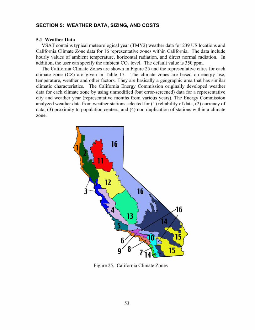
SECTION 5: WEATHER DATA, SIZING, AND COSTS 5.1 Weather Data

VSAT contains typical meteorological year (TMY2) weather data for 239 US locations and California Climate Zone data for 16 representative zones within California. The data include hourly values of ambient temperature, horizontal radiation, and direct normal radiation. In addition, the user can specify the ambient CO2 level. The default value is 350 ppm.

The California Climate Zones are shown in Figure 25 and the representative cities for each climate zone (CZ) are given in Table 17. The climate zones are based on energy use, temperature, weather and other factors. They are basically a geographic area that has similar climatic characteristics. The California Energy Commission originally developed weather data for each climate zone by using unmodified (but error-screened) data for a representative city and weather year (representative months from various years). The Energy Commission analyzed weather data from weather stations selected for (1) reliability of data, (2) currency of data, (3) proximity to population centers, and (4) non-duplication of stations within a climate zone.

Figure 25. California Climate Zones

53

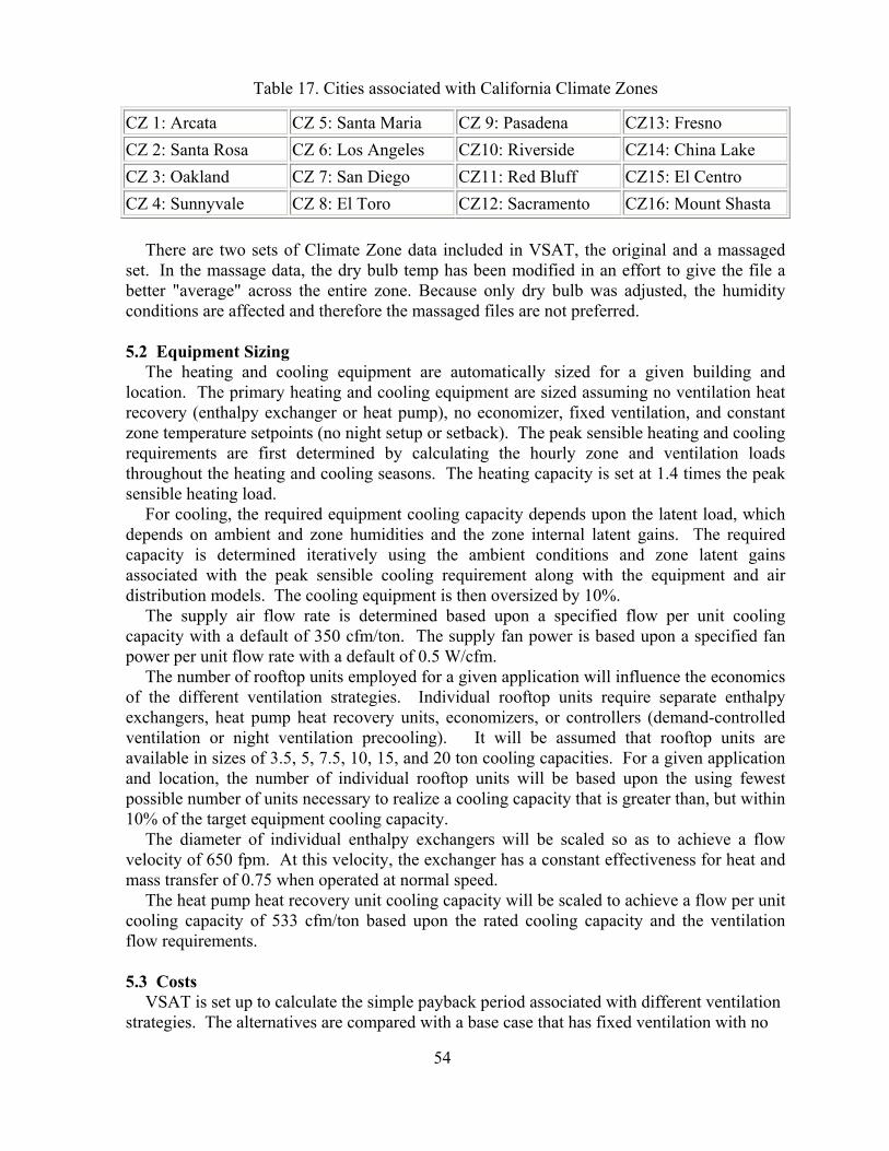
Table 17. Cities associated with California Climate Zones

CZ 1: Arcata CZ 5: Santa Maria CZ 9: Pasadena CZ13: Fresno CZ 2: Santa Rosa CZ 6: Los Angeles CZ10: Riverside CZ14: China Lake CZ 3: Oakland CZ 7: San Diego CZ11: Red Bluff CZ15: El Centro CZ 4: Sunnyvale CZ 8: El Toro CZ12: Sacramento CZ16: Mount Shasta

There are two sets of Climate Zone data included in VSAT, the original and a massaged

set. In the massage data, the dry bulb temp has been modified in an effort to give the file a better "average" across the entire zone. Because only dry bulb was adjusted, the humidity conditions are affected and therefore the massaged files are not preferred. 5.2 Equipment Sizing

The heating and cooling equipment are automatically sized for a given building and location. The primary heating and cooling equipment are sized assuming no ventilation heat recovery (enthalpy exchanger or heat pump), no economizer, fixed ventilation, and constant zone temperature setpoints (no night setup or setback). The peak sensible heating and cooling requirements are first determined by calculating the hourly zone and ventilation loads throughout the heating and cooling seasons. The heating capacity is set at 1.4 times the peak sensible heating load.

For cooling, the required equipment cooling capacity depends upon the latent load, which depends on ambient and zone humidities and the zone internal latent gains. The required capacity is determined iteratively using the ambient conditions and zone latent gains associated with the peak sensible cooling requirement along with the equipment and air distribution models. The cooling equipment is then oversized by 10%.

The supply air flow rate is determined based upon a specified flow per unit cooling capacity with a default of 350 cfm/ton. The supply fan power is based upon a specified fan power per unit flow rate with a default of 0.5 W/cfm.

The number of rooftop units employed for a given application will influence the economics of the different ventilation strategies. Individual rooftop units require separate enthalpy exchangers, heat pump heat recovery units, economizers, or controllers (demand-controlled ventilation or night ventilation precooling). It will be assumed that rooftop units are available in sizes of 3.5, 5, 7.5, 10, 15, and 20 ton cooling capacities. For a given application and location, the number of individual rooftop units will be based upon the using fewest possible number of units necessary to realize a cooling capacity that is greater than, but within 10% of the target equipment cooling capacity.

The diameter of individual enthalpy exchangers will be scaled so as to achieve a flow velocity of 650 fpm. At this velocity, the exchanger has a constant effectiveness for heat and mass transfer of 0.75 when operated at normal speed.

The heat pump heat recovery unit cooling capacity will be scaled to achieve a flow per unit cooling capacity of 533 cfm/ton based upon the rated cooling capacity and the ventilation flow requirements. 5.3 Costs

VSAT is set up to calculate the simple payback period associated with different ventilation strategies. The alternatives are compared with a base case that has fixed ventilation with no

54

economizer or other ventilation strategy. For any alternative k, the simple payback period is calculated as

k

kpb S

CN = (5.1)

where Sk is the annual savings in utility costs associated with the ventilation strategy as compared with the base case and Ck is the installed cost associated with implementing the ventilation strategy.

The annual utility costs associated with operating the HVAC system are calculated according to

( )∑∑

=

=

=

⋅+⋅+

⋅+⋅+⋅=

12

11

,,,,,,

,,,,,,,,,,,,m

m

N

imimigmimie

moffpeakmoffdmmidpeakmmiddmonpeakmond

HVAC m

GrWr

WrWrWrC

&&&

(5.2)

where m is the month, i is the hour, Nm is the number of hours in month m, and for each month m: rd,on,m, rd,mid,m and rd,off,m are the utility rates for electricity demand during the on-peak, mid-peak and off-peak periods ($/kW) and W , and are the peak power consumption for the HVAC equipment during the on-peak, mid-peak and off-peak periods; and for each hour i of month m: r

monpeak ,,&

mmidpeakW ,,&

moffpeakW ,,&

e is the utility rate for electricity usage ($/kWh), W is the electricity usage (kWh), rg is the utility rate for natural gas usage ($/therm), G is the gas usage (therm).

The electricity costs include both energy ($/kWh) and demand charges ($/kW) for on-peak, off-peak, and mid-peak periods. Gas energy usage does not vary with time of the day. However, the user can enter different electric and gas rates for summer and winter periods.

The default rates and periods incorporated in VSAT are given in Table 18, Table 19, and Table 20. The default electric utility rates incorporated in VSAT are based upon Pacific, Gas and Electric Company (PG&E) Schedule E-19. The default natural gas rates are based on PG&E Schedule G-NR1.

Table 18. Default time periods for utility rates

PG&ESummer: May 1 - Oct. 31 Winter: Nov. 1 - April 30On-Peak 12:00 - 6:00, M - F On-Peak N/AMid-Peak 8:30 AM - 12:00 & Mid-Peak 8:30 AM - 9:30 PM, M - F

6:00 PM - 9:30 PM, M - FOff-Peak 9:30 PM - 8:30 AM, all week Off-Peak 9:30 PM - 8:30 AM, all week

Table 19. Default natural gas rates in VSAT

PG&E Schedule G-NR1, CA Climate Zones 1, 2, 3, 4, 11, 12, 13, 1Summer Season $0.67355Winter Season $0.74220

55

Table 20: Default electric rates in VSAT

PG&E Schedule E-19, CA Climate Zones 1, 2, 3, 4, 5, 11, 12, 13Energy Charge - $/kWhSummer Season On-Peak $0.08773

Mid-Peak $0.05810Off-Peak $0.05059

Winter Season On-Peak N/AMid-Peak $0.06392Off-Peak $0.05038

Time Related Demand Charge - $kWSummer Season On-Peak $13.35

Mid-Peak $3.70Off-Peak $2.55

Winter Season On-Peak N/AMid-Peak $3.65Off-Peak $2.55

56

Zhipng Zhong

This table is Kevin’s Origin one, I add CZ10 and CZ15 as separate ones because I have the data. Some other difference as I said in the above table.

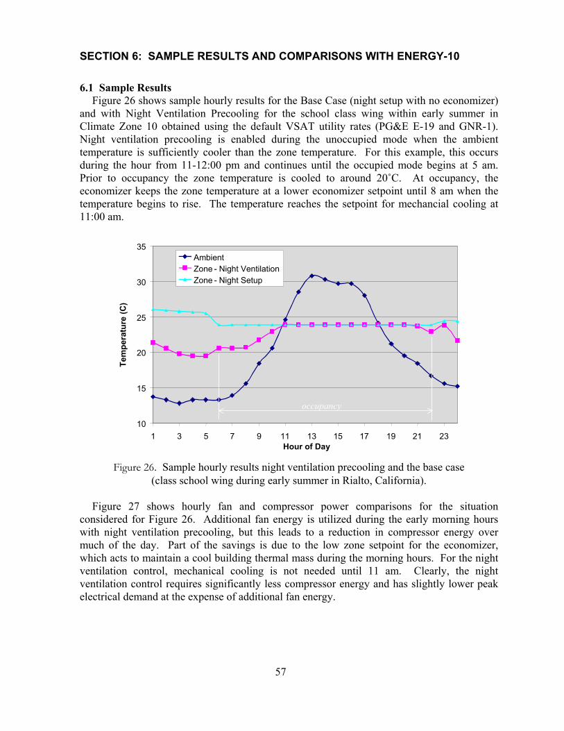
SECTION 6: SAMPLE RESULTS AND COMPARISONS WITH ENERGY-10 6.1 Sample Results

Figure 26 shows sample hourly results for the Base Case (night setup with no economizer) and with Night Ventilation Precooling for the school class wing within early summer in Climate Zone 10 obtained using the default VSAT utility rates (PG&E E-19 and GNR-1). Night ventilation precooling is enabled during the unoccupied mode when the ambient temperature is sufficiently cooler than the zone temperature. For this example, this occurs during the hour from 11-12:00 pm and continues until the occupied mode begins at 5 am. Prior to occupancy the zone temperature is cooled to around 20˚C. At occupancy, the economizer keeps the zone temperature at a lower economizer setpoint until 8 am when the temperature begins to rise. The temperature reaches the setpoint for mechancial cooling at 11:00 am.

10

15

20

25

30

35

1 3 5 7 9 11 13 15 17 19 21 23Hour of Day

Tem

pera

ture

(C)

AmbientZone - Night VentilationZone - Night Setup

occupancy

Figure 26. Sample hourly results night ventilation precooling and the base case

(class school wing during early summer in Rialto, California).

Figure 27 shows hourly fan and compressor power comparisons for the situation considered for Figure 26. Additional fan energy is utilized during the early morning hours with night ventilation precooling, but this leads to a reduction in compressor energy over much of the day. Part of the savings is due to the low zone setpoint for the economizer, which acts to maintain a cool building thermal mass during the morning hours. For the night ventilation control, mechanical cooling is not needed until 11 am. Clearly, the night ventilation control requires significantly less compressor energy and has slightly lower peak electrical demand at the expense of additional fan energy.

57

0

5000

10000

15000

20000

25000

30000

35000

0 2 4 6 8 10 12 14 16 18 20 22 24Hour of Day

Pow

er (W

)

Compressor - Night VentilationCompressor - Night SetupFan - Night VentilationFan - Night Setup

Figure 27: Simulated hourly power for night ventilation precooling and the base case (class school wing during early summer in California Climate Zone 10).

Figure 28 gives annual electrical energy usage for the class school wing in California

Climate Zone 10 for three ventilation strategies: 1) a base case with a night setup thermostat, 2) case 1 with the addition of a differential enthalpy-based economizer, and 3) case 2 with the addition of the night ventilation precooling algorithm. Compared to the base case, the economizer results in a savings in compressor energy of 17.4%. The combined compressor and fan savings are about 11.1%. Compared to the economizer, the addition of the night ventilation algorithm leads to an additional savings of about 14.0% in compressor energy. However, the fan energy increases by about 14.2%, and because the compressor energy is the major consumption, the energy saved in compressor is more than the additional comsumption by fan, the combined savings about 2.6% is achieved compared to the economizer only.

58

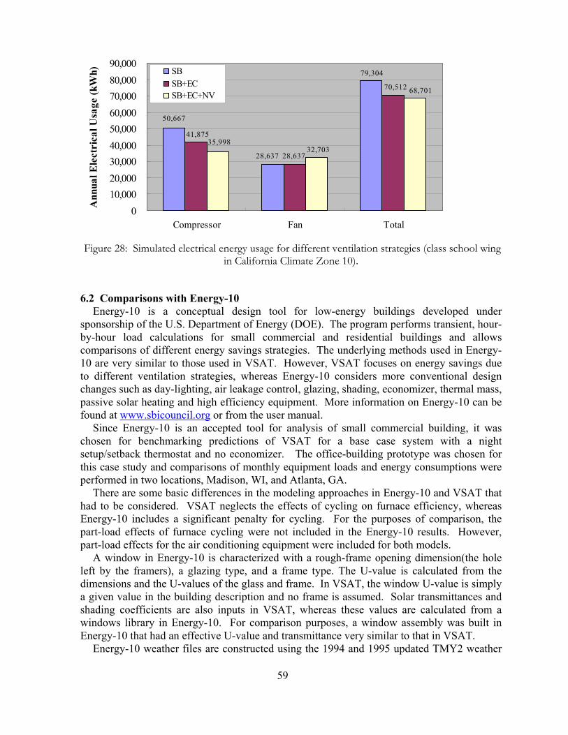
50,667

79,304

28,637

41,875

70,512

28,63732,703

35,998

68,701

010,00020,00030,00040,00050,00060,00070,00080,00090,000

Compressor Fan Total

Ann

ual E

lect

rica

l Usa

ge (k

Wh) SB

SB+ECSB+EC+NV

Figure 28: Simulated electrical energy usage for different ventilation strategies (class school wing in California Climate Zone 10).

6.2 Comparisons with Energy-10 Energy-10 is a conceptual design tool for low-energy buildings developed under

sponsorship of the U.S. Department of Energy (DOE). The program performs transient, hour-by-hour load calculations for small commercial and residential buildings and allows comparisons of different energy savings strategies. The underlying methods used in Energy-10 are very similar to those used in VSAT. However, VSAT focuses on energy savings due to different ventilation strategies, whereas Energy-10 considers more conventional design changes such as day-lighting, air leakage control, glazing, shading, economizer, thermal mass, passive solar heating and high efficiency equipment. More information on Energy-10 can be found at www.sbicouncil.org or from the user manual.

Since Energy-10 is an accepted tool for analysis of small commercial building, it was chosen for benchmarking predictions of VSAT for a base case system with a night setup/setback thermostat and no economizer. The office-building prototype was chosen for this case study and comparisons of monthly equipment loads and energy consumptions were performed in two locations, Madison, WI, and Atlanta, GA.

There are some basic differences in the modeling approaches in Energy-10 and VSAT that had to be considered. VSAT neglects the effects of cycling on furnace efficiency, whereas Energy-10 includes a significant penalty for cycling. For the purposes of comparison, the part-load effects of furnace cycling were not included in the Energy-10 results. However, part-load effects for the air conditioning equipment were included for both models.

A window in Energy-10 is characterized with a rough-frame opening dimension(the hole left by the framers), a glazing type, and a frame type. The U-value is calculated from the dimensions and the U-values of the glass and frame. In VSAT, the window U-value is simply a given value in the building description and no frame is assumed. Solar transmittances and shading coefficients are also inputs in VSAT, whereas these values are calculated from a windows library in Energy-10. For comparison purposes, a window assembly was built in Energy-10 that had an effective U-value and transmittance very similar to that in VSAT.

Energy-10 weather files are constructed using the 1994 and 1995 updated TMY2 weather

59

http://www.sbicouncil.org/

files. This update is based on 30 years of data, rather than 20 years, and incorporates new and improved solar radiation information from the 1992 National Solar Radiation Data Base. The weather data in VSAT used for comparison purposes is TMY data.

The prototypical office was modeled in both Madison and Atlanta. The air-conditioner and furnace equipment models assumed a rated EER of 11 and efficiency of 85%, respectively. In VSAT, the supply fan power was assumed to be 0.5 W/cfm. This value corresponds to a fan efficiency of 11.78% and 0.5 inches H2O system static pressure as entered in Energy-10. Infiltration was neglected for both models. The occupied zone set point for cooling was 23.89°C with a night setup to 29.44°C. The occupied zone set point for heating was 21.11°C with a night setback to 15.56°C.

Table 21 gives equipment sizing determined by VSAT for Madison and Atlanta. These equipment sizes were specified in Energy-10.

Table 21: Equipment Sizing Results from VSAT Office - Madison, WI Office - Atlanta, GA

AC Rated Total Cap., Btu/h 210180 210260AC Rated Sens. Cap., Btu/h 153064 162822Furnace Rated Cap., Btu/h 252924 148583Total Air Flow, cfm 6130 6133Ventilation Air Flow, cfm 924 924Office Floor Area, ft2 6600 6600

Figures 29 – 31 give monthly electricity for the condensing units (compressors and condenser fans), furnace gas input, and supply fan power for both VSAT and Energy-10 in Atlanta, GA. Figures 32 – 34 give similar results for Madison, WI. The trends and absolute magnitudes are very similar for predictions obtained with VSAT and Energy-10. In general, VSAT tends to give slightly higher condensing unit energy and lower gas input energy than Energy-10. Tables 22 and 23 gives tabulated results along with percentage differences between Energy-10 and VSAT for Atlanta and Madison.

60

0

1000

2000

3000

4000

5000

Jan Feb M

ar A

pr M

ay Jun Jul A

ug Sep O

ct N

ov D

ec

kWh Energy-10

VSAT

Figure 29. Monthly Electrical Consumption for Cooling – Atlanta, GA

0

500

1000

1500

2000

2500

3000

Jan Feb M

ar A

pr M

ay Jun Jul A

ug Sep O

ct N

ov D

ec

kWh Energy-10

VSAT

Figure 30. Monthly Furnace Gas Input – Atlanta, GA

0

200

400

600

800

1000

1200

Jan Feb M

ar A

pr M

ay Jun Jul A

ug Sep O

ct N

ov D

ec

kWh Energy-10

VSAT

Figure 31. Monthly Supply Fan Power Consumption – Atlanta, GA

61

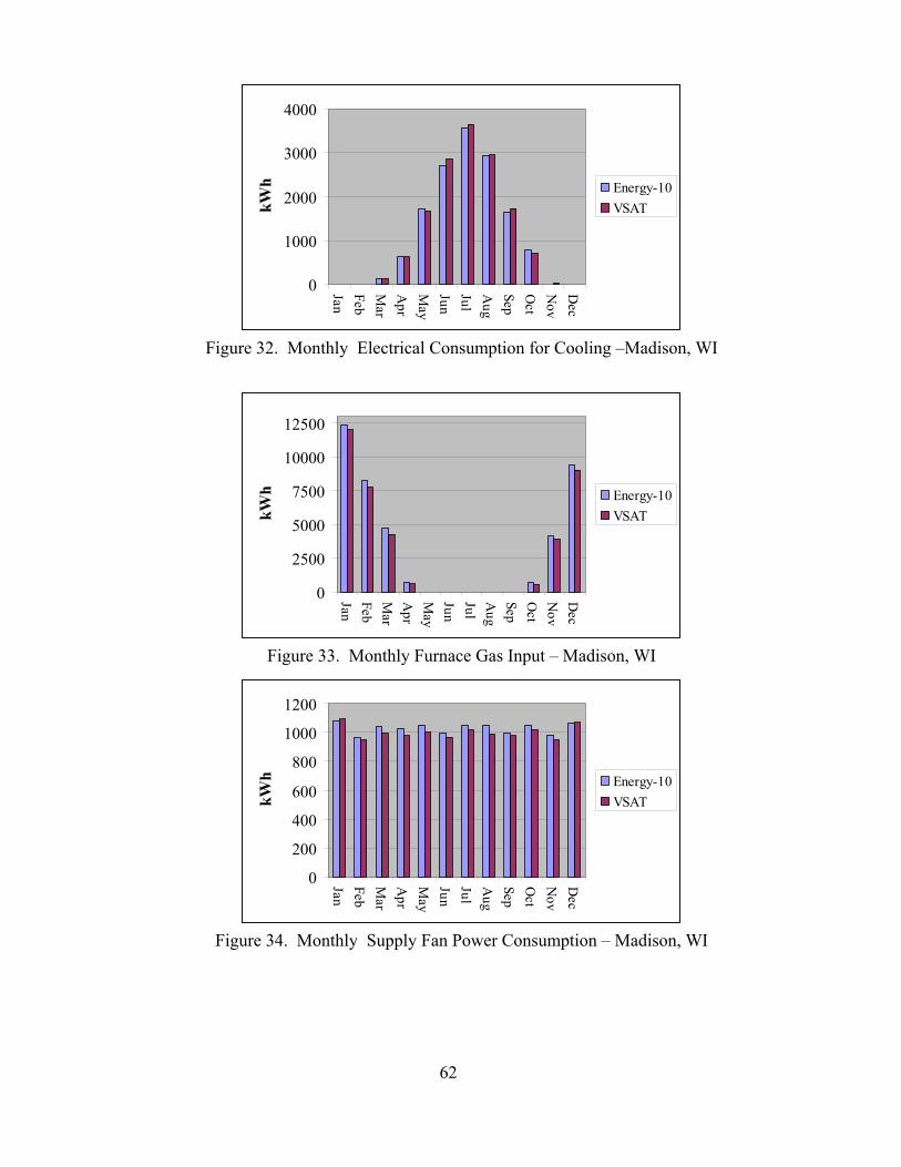
0

1000

2000

3000

4000

Jan Feb M

ar A

pr M

ay Jun Jul A

ug Sep O

ct N

ov D

ec

kWh Energy-10

VSAT

Figure 32. Monthly Electrical Consumption for Cooling –Madison, WI

0

2500

5000

7500

10000

12500

Jan Feb M

ar A

pr M

ay Jun Jul A

ug Sep O

ct N

ov D

ec

kWh Energy-10

VSAT

Figure 33. Monthly Furnace Gas Input – Madison, WI

0

200

400

600

800

1000

1200

Jan Feb M

ar A

pr M

ay Jun Jul A

ug Sep O

ct N

ov D

ec

kWh Energy-10

VSAT

Figure 34. Monthly Supply Fan Power Consumption – Madison, WI

62

Table 22: VSAT and Energy-10 Results – Atlanta, GA

AC kWhr Furnace kWhr Fan kWhr Month Energy-10 VSAT Energy-10 VSAT Energy-10 VSAT

Jan 168 139 2712 2589 1038 1020 Feb 397 407 1851 1738 937 909 Mar 968 849 171 142 1037 987 Apr 1828 1878 78 74 1031 981 May 2905 3021 0 0 1053 1003 Jun 3474 3790 0 0 1000 966 Jul 4448 4570 0 0 1054 1018

Aug 4050 4173 0 0 1054 987 Sep 3144 3398 0 0 999 981 Oct 1898 1905 0 0 1053 1018 Nov 662 650 332 345 982 951 Dec 330 258 2118 1815 1037 1018 Yr 24272 25038 7262 6703 12275 11839

AC error 3.06% Furnace error -8.35% Fan error -3.68%

Table 23: VSAT and Energy-10 Results – Madison, WI AC kWhr Furnace kWhr Fan kWhr

Month Energy-10 VSAT Energy-10 VSAT Energy-10 VSAT Jan 0 0 12378 12018 1082 1092 Feb 5 0 8247 7779 960 948 Mar 110 128 4779 4264 1039 994 Apr 622 618 711 622 1030 981 May 1716 1664 11 12 1053 1002 Jun 2705 2852 0 0 998 966 Jul 3561 3636 0 0 1054 1018

Aug 2934 2943 0 0 1053 987 Sep 1650 1728 0 18 998 981 Oct 766 687 694 523 1053 1018 Nov 2 20 4178 3927 982 951 Dec 0 0 9414 9023 1065 1070 Yr 14070 14276 40412 38186 12367 12008

AC error 1.44% Furnace error -5.83% Fan error -2.99%

63

SECTION 7: REFERENCES

ASHRAE. 2000. ASHRAE Handbook: HVAC Systems and Equipment, Atlanta: American Society of Heating, Refrigerating and Air-Conditioning Engineers, Inc.

ASHRAE. 1999. “ANSI/ASHRAE Standard 62-1999, “Ventilation for Acceptable Indoor Air Quality”, Atlanta: American Society of Heating, Refrigerating and Air-Conditioning Engineers, Inc.

ASHRAE. 1993. ASHRAE Handbook: Fundamentals, Atlanta: American Society of

Heating, Refrigerating and Air-Conditioning Engineers, Inc. Brandemuehl, M.J. and Braun, J.E., “The Impact of Demand-Controlled and Economizer

Ventilation Strategies on Energy Use in Buildings, ASHRAE Transactions, Vol. 105, Pt. 2, pp. 39-50, 1999.

Brandemuehl, M.J., Gabel, S., and Andresen, I. 1993. HVAC2 Toolkit: Algorithms and

Subroutines for Secondary HVAC System Energy Calculations. American Society of Heating, Refrigerating, and Air Conditioning Engineers, Inc., Atlanta, GA.

Braun, J.E. and Brandemuehl, M.J. 2002. Savings Estimator Technical Reference

Manual. Carrier Corporation. 1999. “Product Data: 62AQ Energy$Recycler Energy Recovery

Accessory For 3 to 12.5 Ton Rooftops”, Form 62AQ-1PD. Syracuse, New York.

Carnes Company. 1989. “Energy Recovery Wheel Design Manual,” Verona, WI. Chaturvedi, N. and Braun, J.E. “An Inverse Gray-Box Model for Transient Building Load

Prediction,” International Journal of Heating, Ventilating, Air-Conditioning and Refrigeration Research, Vol. 8, No. 1, pp. 73-100, 2002.

Duffie, J.A. and Beckman, W.A., Solar Engineering of Thermal Processes, Wiley—

Interscience, 1980. DOE-2. 1982. Engineer’s Manual, Version 2.1A. Lawrence Berkeley Laboratory and

Los Alamos National Laboratory.

Huang, Y.J., Akbari, H., Rainer, L., and Ritschard, R.L. 1990. 481 Prototypical Commercial Buildings for Twenty Urban Market Areas (Technical documentation of building loads data base developed for the GRI Cogeneration Market Assessment Model). LBL Report 29798, Lawrence Berkley National Laboratory, Berkley CA.

Huang, Y.J., and E. Franconi. 1995. Commercial Heating and Cooling Loads Component Analysis. LBNL Report 38970, Lawrence Berkeley National Laboratory, Berkeley,

CA.

64

65

Kays, W.M., and M.E. Crawford. 1980. Convective Heat and Mass Transfer. New York: McGraw-Hill.

Klein, H., Klein, S.A., and Mitchell, J.W., 1990, “Analysis of regenerative enthalpy

exchangers,” International Journal of Heat and Mass Transfer, Vol. 33, No.4, pp. 735-744.

Maclaine-cross, I.L. 1974. A Theory of Combined Heat and Mass Transfer in

Regenerators. Ph.D. Thesis in Mechanical Engineering, Monash University, Australia.

Seem, J.E., Klein, S.A., Beckman, W.A., and Mitchell, J.W., 1989, “Transfer functions for

efficient calculations of multi dimensional heat transfer,” Journal of Heat Transfer- Transactions of the ASME, Vol. 111, No.1, pp. 5-12.

Stiesch, G., S.A. Klein, J.W. Mitchell. 1995. Performance of Rotary Heat and Mass

Exchangers. HVAC&R Research 1(4): 308-324. TRNSYS. 2000. TRNSYS Users Guide: A Transient Simulation Program. Solar Energy

Laboratory, University of Wisconsin-Madison.

VENTILATION STRATEGY ASSESSMENT TOOL · SECTION 1: INTRODUCTION This report describes a simulation...

Documents

Transcript of VENTILATION STRATEGY ASSESSMENT TOOL · SECTION 1: INTRODUCTION This report describes a simulation...