Vehicle Tracking and Motion Prediction in Complex Urban Scenarios

Christoph Hermes, Julian Einhaus, Markus Hahn, Christian Wohler and Franz Kummert

Abstract— The recognition of potentially hazardous situa-tions on road intersections is an indispensable skill of futuredriver assistance systems. In this context, this study focuseson the task of vehicle tracking in combination with a long-term motion prediction (1–2 s into the future) in a dynamicscenario. A motion-attributed stereo point cloud obtained usingcomputationally efficient feature-based methods represents thescene, relying on images of a stereo camera system mounted on avehicle. A two-stage mean-shift algorithm is used for detectionand tracking of the traffic participants. A hierarchical setupdepending on the history of the tracked object is applied forprediction. This includes prediction by optical flow, a standardkinematic prediction, and a particle filter based motion patternmethod relying on learned object trajectories. The evaluationshows that the proposed system is able to track the road usersin a stable manner and predict their positions at least oneorder of magnitude more accurately than a standard kinematicprediction method.

I. INTRODUCTION

Future driver assistance systems will have to be able to

interpret complex traffic situations and will therefore have to

estimate and predict the position and motion state of the ego-

vehicle and other vehicles surrounding it over time intervals

of several seconds. Such information will e.g. allow to assess

the risk of an upcoming situation.

A long-term prediction method requires adequate motion

history knowledge for each vehicle in the scene. Especially

for noisy 3D point data from a stereo camera system (cf.

Fig. 1(b)) the application of a tracking method is favourable

for minimising the effects of noise over time. It is common

to use a Kalman filter approach [1] with a manually defined

motion model for the prediction part, but this approach often

lacks adaptation speed when the object rapidly changes its

driving behaviour. Instead, we apply a modification of the

particle filter framework proposed in [2], where the motion

model is defined by recorded motion patterns, and extend

this method by the simultaneous detection of several objects,

such that the particle filter is able to track several motion

hypotheses for each traffic participant in parallel.

For this contribution, we have chosen a roundabout as a

test scenario as it includes several different motion patterns

normally found in urban traffic: For traffic participants at

large distances to the sensor (about 30–50 m), small errors

in the stereo point cloud computation lead to a considerable

C. Hermes and F. Kummert are with the Faculty ofTechnology, Bielefeld University, Bielefeld, Germany, {chermes,franz}@techfak.uni-bielefeld.de

J. Einhaus and M. Hahn are with Daimler AG, Group Research, Ulm, Ger-many, {Julian.Einhaus, Markus.Hahn}@daimler.com

C. Wohler is with the Image Analysis Group, Dort-mund University of Technology, Dortmund, Germany,christian.woehler@tu-dortmund.de

(a) Left image from stereo camera setup.

(b) Corresponding motion-attributed 3D point cloud (top view).

Fig. 1. Roundabout scenario.

amount of noise [3]. Additionally, the vehicles often occlude

each other. Objects passing by in front of the camera are

visible only for short periods of time, about 3–4 s. In this

case, a tracking algorithm based on temporal filtering has

very little time to settle its parameters. Turning vehicles yield

high dynamics compared to a simple turn at intersections,

which tends to be difficult to follow for a standard filter.

The issue of vehicle tracking has been addressed by many

researchers in the past decades and a complete overview

would be out of the scope of this paper. For the interested

reader in the field of object tracking in general, we refer

to the excellent surveys by Lepetit and Fua [4] and by

Yilmaz et al. [5]. Numerous works in the domain of vehicle

tracking deal with the Kalman filter approach [1] and its

common extensions like the Extended Kalman filter (EKF)

or the Unscented Kalman filter (UKF). Various features are

used for tracking. Melli et al. [6] detect stopping vehicles

with two-dimensional boxes in images based on an extension

of the Kalman filter. Background and shadow classification

are handled separately. A multiple filter setup is used by

Barth and Franke [7], where each three-dimensional object

point is assigned an individual Kalman filter and is tracked

over time. A vehicle is represented by such a point cloud

and segmented based on a cuboid model. Active contours

and silhouettes are also widely used for vehicle tracking.

Yokoyama and Poggio [8] combine edge features and optical

flow for object tracking with active contours. Similarly,

Luo and Bhandarkar [9] present a tracking approach based

on regions and contours, where velocity fields are used in

order to approximate the object contour by B-spline surfaces

combined with a Kalman filter.

Other works in the field of vehicle tracking include

the tracking-by-detection method [3] and tracking of non-

parametric probability densities. For example, Comaniciu

et al. [10] use histograms together with a mean-shift algo-

rithm on RGB color features to track people in dynamic

scenes. Heisele [11] uses colour and optical flow features

for tracking clusters in images. These clusters are used to

form motion trajectories for generating object hypotheses.

Schiele [12] finds homogeneous regions in images by using

a k-means clustering in color space. Objects or object parts

are combined and tracked with a Viterbi-based tracking

algorithm for similarly moving regions. A vehicle tracking

method based on 3D models is presented in [13], [14].

Relying on the association of edge elements and optical flow,

the models are applied to vehicles appearing small in images

acquired with a traffic surveillance camera. Support Vector

Machines (SVMs) are used by Avidian [15] for a stable

tracking of vehicle rear ends in traffic. The classification

is performed in images taken with a monocular camera

mounted on the ego-vehicle.

Hidden Markov Models (HMMs) are another well-

established state estimation and tracking method for vehicles.

Fraile and Maybank [16] estimate discrete states of the

vehicle for classifying the movement of the tracked object.

Yin et al. [17] use a HMM for vehicle part detection and

track them in congested traffic over time.

A few researchers have addressed the topic of vehicle state

prediction based on previously observed motion patterns:

Johnson and Hogg [18] represent a set of pedestrian tra-

jectories using a neural network combined with vector quan-

tisation. They suggest an event recognition and prediction

method using probability densities which are determined by

the distribution of the prototype vectors. Sumpter et al. [19]

propose a long-term spatio-temporal prediction method for

a flock of animals in the presence of a predator based on

observed trajectories and flock shapes. Similar to [18], the

authors utilise a neural network combined with vector quanti-

sation to cluster the motion data. The prediction is performed

by a recursive loop where in each iteration the winning

neuron is predicted into the next time step by the network.

Hu et al. [20] determine image-based trajectories of vehicles

Fig. 2. System overview.

using foreground classification and a exponential smoothing-

based prediction method. A hierarchical clustering algorithm

is applied to retrieve typical motion patterns from a given

set of trajectories. Each motion pattern is represented by a

chain of Gaussian distributions which are used for statistical

anomaly detection and behaviour prediction.

An overview of the tracking and prediction method pro-

posed in this study is shown in Fig. 2. A 3D bounding box

model represents a vehicle in the scene (cf. Section II). The

environment of the observer is represented by a motion-

attributed 3D point cloud. New objects entering the scene are

detected by graph-based clustering and verified for further

time steps by a two-step mean-shift algorithm (cf. Sec-

tion III). For tracking, we apply a hierarchical prediction

method depending on the length of the observed motion his-

tory (cf. Section IV). The tracking and long-term prediction

approaches are evaluated quantitatively in Section V.

II. OBJECT AND MOTION MODEL

The ego-vehicle observes the environment with a stereo

camera sensor. Each traffic participant (e.g. vehicles and

bicycles) is assumed to be a rigid object, i.e. shape defor-

mations do not occur during tracking. Pedestrians are not

considered in the proposed method because their motion

is difficult to predict even by a human driver. An object

is represented as a three-dimensional bounding box Φ =[cx,cz,sx,sy,sz]

T covering the rough shape of the object.

The dimensions x, y and z denote the lateral, elevation,

and longitudinal axis, respectively, according to the camera

coordinate system. The box model includes the projected

centre c = [cx,cz]T to the ground and is aligned parallel to

the image plane of the camera system. Therefore the object

dimension [sx,sy,sz]T denotes the spatial extension according

to the camera coordinate axes.

In this study, motion patterns from a training set are com-

pared with the observed history of a tracked object. Similar

to [2], a motion pattern is represented as a trajectory T which

consists of ordered tuples T = ((Φ(1),t1), . . . ,(Φ(N),tN)).This combines the object state Φ(id) with a time stamp t(id).

The object orientation (yaw angle) and higher derivatives

like the yaw rate and velocity can be inferred from the first

two dimensions of the object state Φ over time by numerical

computation of the temporal derivatives.

III. OBJECT DETECTION

The idea behind the tracking system is to extract the

motion patterns of all moving objects in the observed scene.

For this purpose their 3D positions and motion states have

to be estimated (cf. Section III-A). We use a standard stereo

two-camera setup with a baseline of 220 mm for three-

dimensional environment perception. The stereo camera sys-

tem is calibrated and the images are rectified to standard

epipolar geometry. When a vehicle enters the scene, the

proposed system sets up a new tracking model based on

an initially detected object (cf. Section III-B). Additionally,

the system generates a “target model” for tracking the

object both in the camera images (image-based mean-shift,

cf. Section III-C) and in the 3D point cloud (point cloud-

based mean-shift, cf. Section III-D).

A. Sparse Scene Flow

Object detection and 3D tracking are based on a sparse

scene flow field. We use a combination of sparse correlation-

based stereo and sparse optical flow. Both algorithms are

based on the computationally efficient correspondence esti-

mation method described by Stein [21], where corresponding

feature points in the images of the left and the right camera

are used to obtain the 3D points and the current and previous

camera images are used to compute the optical flow field.

The optical flow field vectors are assigned to the 3D points

by computing the mean velocity in a small neighbourhood

(2 pixels radius) of the spatial points in the image plane. This

results in a motion-attributed point cloud, better known as the

scene flow field (Fig. 3(a)). Therefore, each scene flow point

si = [si,x,si,y,si,z, si,x, si,y]T has a spatial part [si,x,si,y,si,z]

T

and a velocity part [si,x, si,y]T . In contrast to classical scene

flow [22], the longitudinal velocity part si,z of the stereo

points is not determined. This drawback is compensated

by the high computational efficiency of the correspondence

estimation method.

A graph based clustering algorithm according to [23] is

used to separate differently moving groups of 3D points from

each other. First the moving objects are separated from the

stationary ones by taking only those points from the scene

flow point set S = {s1, . . . ,sM} with a velocity ‖[si,x, si,y]T‖>

εv relative to the stationary environment, which results in a

reduced scene flow point set Sεv ⊆ S. Objects standing still

when entering the sensors field of view will be considered as

stationary objects. A cluster A⊆ Sεv can be defined as a point

set with maximum similarity whereas the similarity between

different clusters is minimised. For each point si ∈ Sεv\A a δ -

vicinity exists such that si is added to A if ∃s j ∈A : d(s j,si)<δ , where d(·, ·) denotes the Euclidean distance metric and δis a distance threshold. This procedure is repeated for all

si ∈ Sεv until no point can be added to A any more. The next

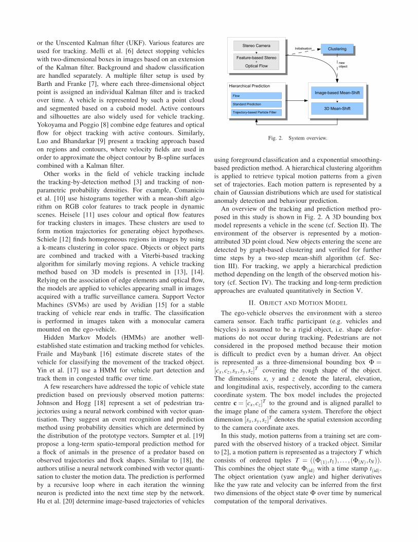
clusters are computed correspondingly. For illustration, the

colour of each 3D point in Fig. 3(b) is chosen according to

its cluster assignment.

Tracked vehicles may reduce their speed or stop com-

pletely, especially at intersections. Hence, a cluster will not

always be detected, such that it cannot be used as the only

(a) 3D point cloud (blue) and as-signed velocities (green).

(b) Clustering result.

Fig. 3. Scene flow and clustering result (top view).

tracking feature. We therefore use the image grey values as

additional tracking features.

B. Model Initialisation

For each object in the scene, the tracking system requires

an initial pose. This step is necessary when a previously

unseen object enters the scene or when the track is lost

because of multiple mutual occlusions, such that the object

appears at unexpected locations. For this purpose we apply

the clustering method at each time step: When a cluster is

found which cannot be assigned to an existing tracked object,

i.e. the distance value exceeds a threshold dobj, a new model

Φ(id)(t0) is set for this cluster and tracked over the following

time steps t > t0. The cluster centre projected to the ground

serves as the model centre and the initial model dimensions

are determined by a bounding box around a cluster.

As mentioned before, the cluster method is not suitable to

serve as the only tracking feature due to the fact that clusters

are missing over several frames. In addition, the objects are

tracked both in the camera images and in the original point

cloud, where the image grey values are used to weight each

3D point. This weighting is based on a target model q(id) for

each object (id) consisting of a grey value histogram with

256 bins. Assuming that all three-dimensional points on the

model Φ(id) have the same depth value, a three-dimensional

model projection onto the camera images simplifies to the

projection of a parallel plane. This means that each visible

three-dimensional model point can be projected efficiently

into the camera images. The histogram q(id) is first computed

by the projection of the initial model Φ(id)(t0) into each

camera image and is updated incrementally in the following

time steps using

q′(id)(t + 1) = α · q(id)(t)+ (1−α) · q(id)(t + 1). (1)

The target model is normalised such that ∑256j=1 q

( j)i = 1 and

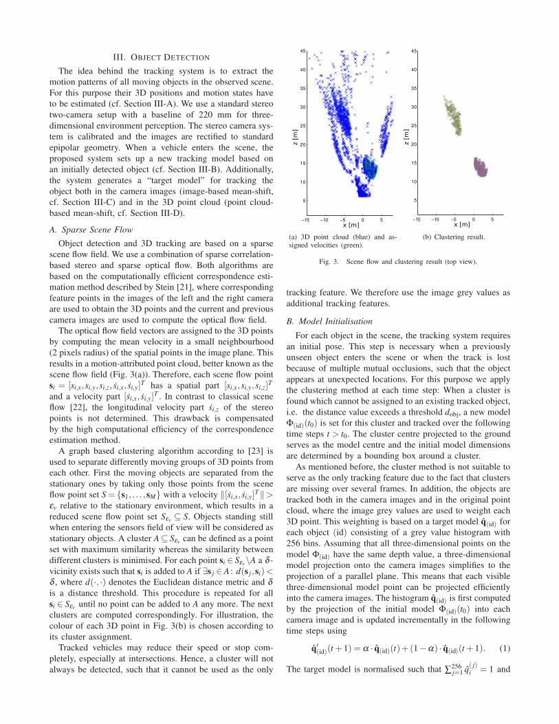
Fig. 4. Image-based mean-shift: 3D grid parallel to stereo image layers.Each grid cell is projected into the stereo images and weighted with thecorresponding grey values.

is interpreted as an occurrence probability for each grey

value. An image-based mean-shift algorithm looks for the

most likely image region in the following time steps by

comparing the grey value histograms. Since the histogram

contains no spatial information, the object tracking is robust

against object rotations and illumination changes.

C. Image-based Mean-shift

A target model q(id)(t) of the corresponding object model

Φ(id)(t) is used to guide a mean-shift algorithm inside a

search window to the object centre. This method is based

on the CAMShift algorithm proposed by Bradski [24], but

instead of specifying the search window to be in image co-

ordinates, we look for the mean object centre in 3D space by

defining a grid parallel to the image plane as shown in Fig. 4.

The three-dimensional cell size of the grid corresponds to the

projected pixel size in both camera images. For each grid cell

gCelli(xi) with mean centre xi an intensity value is assigned

by projecting xi into both camera images I(1,2), yielding the

image coordinates ui, and taking the mean grey value:

gCelli(xi) =1

2[I1(ui)+ I2(ui)]. (2)

A look-up in the target model histogram results in an

occurrence probability qi(gCelli) for each grid cell gCelli.

The 3D centre point c is estimated with the mean-shift

procedure using a geometric rectangle model. This mean-

shift state allows only for an update of the lateral pose of

the tracked object, since the probability grid is parallel to

the image plane. No information from the scene flow field is

used, such that a pose update of the rectangle is computed

even if there is no new 3D information available.

D. Point Cloud based Mean-shift

In this stage all moving 3D points of the scene flow field

are used to update the 3D pose of the tracked box. At the

first iteration j = 1 of the mean-shift procedure the box centre

c j=1 is initialised with the estimated 3D centre point c of the

image-based mean-shift stage. For all subsequent iterations,

the box model is moved to the new position

c j+1 =∑N

n=1 sn ·g(sn,c j) · q(id)(gCelli(sn))

∑Nn=1 g(sn,c j) · q(id)(gCelli(sn))

(3)

where c j is the previous centre position. In the mean-shift

procedure we use a truncated Gaussian kernel [25]

g(sn,c j) =

{

e−β ||sn−c j ||2

if ||sn − c j||2 ≤ λ

0 otherwise(4)

where β denotes the kernel width and λ defines the maxi-

mum allowed distance of ||sn − c j||2 and is typically chosen

such that∫ λ

0 e−β ||sn−c j ||2

covers 99% of the area under the

Gaussian kernel function.

Our mean-shift based 3D tracking approach incorporates

an appearance weighting q(id)(gCelli(sn)) obtained by look-

ing up the appearance probability of the moving 3D point

sn in the target model q(id), such that a 3D point with an

appearance similar to the target appearance is assigned a

higher weight.

IV. OBJECT TRACKING

For a driver assistance system not only the position of

other traffic participants but also their future behaviour is im-

portant, i.e. where the other objects will be in the subsequent

time steps. In this context, our previous work [2] presents

a long-term (∼ 2 s ahead) behaviour prediction method,

but it is assumed that a motion history (≥ 30 frames) has

already been observed. This assumption cannot be directly

applied here, because new objects entering the scene have

no observed motion history. Therefore, we extend the work

in [2] by a hierarchical prediction method whose application

depends on the length of the motion history. For newly

detected objects a simple flow-based prediction is applied

(cf. Section IV-A). Once the history length of a tracked

object exceeds a predefined threshold l1 we use a so-called

kinematic prediction (cf. Section IV-B), which yields the

approximate motion direction. Similarly, the trajectory-based

prediction method (cf. Section IV-C) is applied when the

history length is larger than a threshold l2 with l2 > l1 and

is used for the prediction step in the tracking system as well

as for a long-term prediction of the object state. In general,

the prediction becomes more stable with increasing length

of the motion history.

For each traffic participant a new tracker instance is

created when the system detects an object. Because the stereo

cameras have a similar field of view as the driver, mutual

occlusions between the traffic participants often occur. Es-

pecially when an object passes a row of vehicles in the rear

area of the observed scene, the object cannot be found by

the detector. Therefore we set an occlusion flag when an

object is hidden, which causes the tracker to disable the

object detection step for the corresponding frame.

A. Flow-Based Prediction

The flow-based prediction utilises the velocity information

from the scene flow field. An object Φ(id)(t−1) is predicted

to the current time step t using the linear equation

Φ(id)(t) = Φ(id)(t −1)+ [vi ·∆t,0,0,0]T , (5)

where vi is the median velocity of all scene flow points si

inside the box model Φ(id)(t − 1) and ∆t denotes the time

difference between two successive frames. Zero values in (5)

indicate the absence of change in the box model dimensions.

Note that vi is a two-dimensional vector parallel to the

camera image planes because the optical flow yields no depth

information. It is assumed that the point cloud based mean-

shift can handle the depth adjustment sufficiently well.

B. Kinematic Prediction

The kinematic prediction is an extrapolation technique

assuming constant acceleration and curve radius with respect

to the current vehicle state. This prediction yields a circular

path on which the vehicle performs a constantly accelerated

motion. Although the acceleration based on the tracked

object path is sensitive to noise, the curve radius has more

influence on the kinematic prediction model since it affects

the motion direction. This simple kinematic model allows

good predictions for time intervals of a few tenths of a second

but yields unrealistic and inaccurate results when performing

a long-term prediction for time intervals of several seconds.

C. Trajectory Particle Filter

The trajectory-based prediction utilises a set of previ-

ously observed motion patterns (i.e. reference trajectories)

and finds the most probable hypotheses (sub-trajectories)

to represent the current object motion history based on the

longest common subsequence (LCS) [26]. Each hypothesis

is weighted by the quaternion-based rotationally invariant

longest common subsequence (QRLCS) metric [2]. This

metric compares the difference between two trajectories and

finds the best matching subsequence in each compared tra-

jectory while preserving the optimal transformation (rotation

and translation in the 2D plane) of one sub-trajectory to the

other.

The LCS can be computed with the dynamic programming

(DP) algorithm using tables in which partial (optimal) results

of the algorithm are stored. The optimal, partial translation

and rotation is obtained by regarding the trajectories as two

point sets in which the point-to-point assignments are given

by the DP table. Hence, the rotation angle and the mean

values for each point set are computed incrementally.

The best translation of a trajectory A to a trajectory B can

be obtained using the mean values µa and µb. The mean µa

of point set {ai} is computed incrementally by

µa,T =(T −1)

Tµa,T−1 +

1

TaT (6)

with T as the number of point assignments (analogous for

point set {bi}). For the optimal rotation, a closed-form solu-

tion for the least-squares problem of absolute orientation with

quaternions is given in [27]. A quaternion can be considered

as a complex number with three different imaginary parts

or the combination of a scalar with a 3D Cartesian vector,

q = q0 + iqx + jqy + kqz ≡ [q0,q]. It can be used as a rota-

tion operator on a three-dimensional vector x according to

[0,xR] = q[0,x]q−1, where vectors are treated as quaternions

with zero scalar component. A rotation quaternion can be

constructed based on the rotation angle θ and the three-

dimensional rotation vector n:

q =

√

1 + cosθ

2+

sinθ√

2(1 + cosθ )(inx + jny + knz) (7)

Because of the reasonable flat-world assumption the rotation

vector can be set to the fixed value n = [0,0,1]. For the

rotation in a plane, the rotation vector is constructed in [27]

from two given point sets using

sinθ = S/√

S2 +C2 cosθ = C/√

S2 +C2. (8)

By rotating the point sets (trajectories) up to an assignment

T around their mean centres µa,T and µb,T , the auxiliary

variables S and C become

ST =

⟨(

T

∑t=1

(at ×bt)−T (µa,T × µb,T )

)

,n

⟩

(9)

CT =T

∑t=1

〈at ,bt 〉−T⟨

µa,T ,µb,T

⟩

, (10)

where 〈·, ·〉 and × denote the dot product and the cross prod-

uct, respectively. As a result, only the incremental parts µa,T

and µb,T (Eq. (6)), ∑Tt=1(at ×bt) (Eq. (9)), and ∑T

t=1 〈at ,bt〉(Eq. (10)) have to be stored for each assignment test in the

DP table to guarantee the best rotation and translation.

Similar parts of the reference trajectories are taken as

hypotheses and tracked over time by a particle filter frame-

work. The prediction step is then a simple lookup in the

future trajectory point of the corresponding hypothesis. This

results in multiple object state predictions, where for a single

prediction the mean value of the predictions of all hypotheses

is taken. This method is also applied to obtain predictions

for longer time intervals into the future.

The reference trajectories incorporate all information

about the object state Φ at each trajectory element. For this

reason there is no need for an explicit motion model since

the observed trajectories also cover the state noise. This set

of motion patterns is obtained by tracking traffic participants

while they are inside the field of view without using the

trajectory-based prediction step.

V. EVALUATION

The evaluation of the proposed tracking system is based

on eight sequences of rectified stereo image pairs of a

roundabout. Each sequence is recorded with a frame rate of

42.0 ms/frame and has an approximate length of 250 frames.

To be able to track such relatively long sequences, the

observing vehicle with the mounted stereo camera system

stands in front of the roundabout. For a moving vehicle, ego-

motion compensation e.g. according to [7] would have to be

Fig. 5. Motion patterns extracted by our approach.

applied. We take six sequences for motion pattern extraction

from non-occluded traffic participants for the training set

of the trajectory-based particle filter. The remaining two

sequences (in the following labelled as A and B) are used

for testing and contain 1127 object positions to be tracked in

500 frames. The motion pattern extraction makes use of the

previously described two-stage mean-shift algorithm with the

flow-based and kinematic prediction method. This results in

44 trajectories (cf. Fig. 5) for the training set. Each trajectory

point represents the box model φ i.

In the tracking system, we use an update rate α = 0.2(Eq. (1)), a velocity threshold εv = 2.3 m/s for clustering,

and a δ -vicinity value of 0.5 m. We set the Gaussian kernel

width to β = 0.8 ·min{sx,sy,sz}, i.e. its value depends on

the tracked object dimension. In the hierarchical prediction

method, we apply the flow-based prediction if the trajectory

history is shorter than 5 frames (0.21 s), the kinematic

prediction is applied to a trajectory history in the range

5–30 frames (0.21–1.26 s), and the particle filter is used

for history lengths ≥ 30 frames (1.26 s) with 200 particles,

where only the last 30 frames are taken into account.

The evaluation consists of two parts, where first the

tracking performance is compared with manually labelled

ground truth, and then the prediction capability for several

time steps ahead is shown for the trajectory particle filter.

A. Tracking Results

3D ground truth of the objects in the scene is not available,

i.e. their distance to the camera is unknown. For an adequate

quality assessment of the proposed tracking system, the

object positions are labelled manually as bounding boxes,

resulting in the centre of the object and its dimensions in

the two-dimensional image plane. The 3D object model Φ(id)

detected by the tracking system is then projected into the

camera images and compared with the manually labelled

boxes. At time step t, we define the tracking quality as a

function of the overlap in the horizontal direction according

to

E(Φ(id)(t),O(id)(t))=

{

1 ifoverlap(O(id)(t),Φ(id)(t))

min{w(O(id)(t)),w(Φ(id)(t))}> εo

0 otherwise,(11)

Fig. 6. Tracking quality function example for a manually labelled objectO(id) (yellow) and a tracked object Φ(id) (green).

where O(id) is the manually assigned ground truth of the

tracked object Φ(id), overlap(·, ·) denotes the horizontal over-

lap in pixel units of the boxes, and w(·) is the horizontal

dimension (width) of the bounding box in image coordinates.

The overlap threshold εo is set to 0.1. An example is

depicted in Fig. 6. The tracking results differ depending on

the kind of motion at the roundabout as mentioned in the

introduction. We divide our test set of motion trajectories

into three categories depending on their general motion type

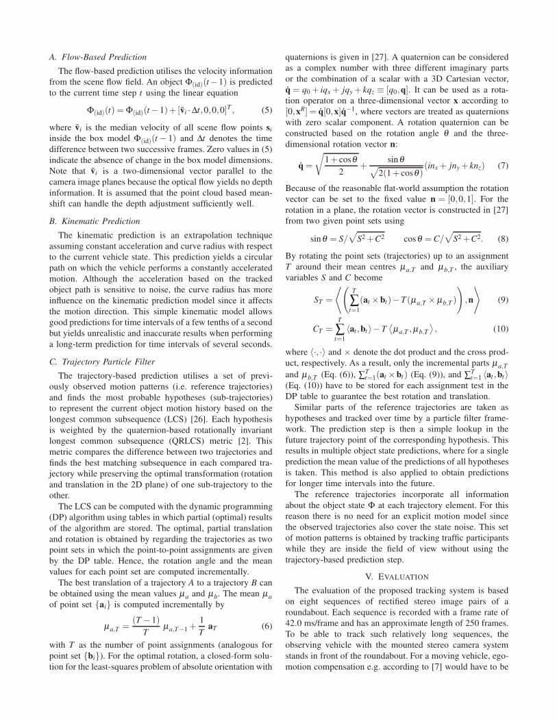
(cf. Fig. 7):

• Category I: Objects which enter the roundabout ∼ 40–

50 m ahead in the left side of the image and drive

closely along the observing vehicle by moving towards

the right side of the image. (6 cars, 1 cyclist)

• Category II: Objects driving from the right to the left

side ∼ 35 m ahead. (8 cars)

• Category III: Objects which enter the scene on the

right side of the image and follow the path through the

roundabout. (3 cars)

We evaluate the proposed tracking system in each category

and in both test sequences A and B for two prediction

methods. The objects are tracked over time by the flow-

based and kinematic prediction method (“kin.” in Table I) and

by all predictions methods, including the trajectory particle

filter (PF). Table I shows the median tracking percentage per

object with the corresponding 25% and 75% quantiles.

Between the categories and sequences there is no major

difference in the median tracking result. However, using the

trajectory particle filter method often leads to a reduction of

the tracking error, which means that the objects are tracked

in a more stable manner. In sequence B, the objects of

category II cannot be tracked. This is due to the fact that

especially in this sequence objects are occluded by objects

from category I most of the time, which means that the

tracking system is not able to build up a stable motion

history, such that hardly any measurements are provided by

the object detection stage and no sufficiently long motion

history is available for a stable tracking.

In sequence A, objects of category I are tracked only

half of the time they are present in the scene for both

prediction approaches used in the tracking system. In this

case, a queue of cars enters from the left hand side at

a distance of approximately 40 m, where the cars follow

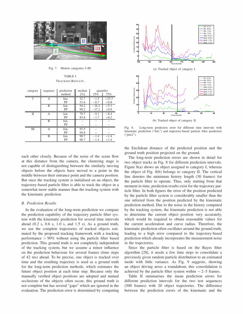
Fig. 7. Motion categories I–III.

TABLE I

TRACKING RESULTS.

category sequence prediction median quantilesmethod [%] 25% 75%

I A kin. 52.7 −1.5 +23.3PF 51.6 −0.7 +0.8

B kin. 94.2 −16.2 +5.1PF 99.2 −17.1 +0.9

II A kin. 79.7 −9.1 +8.4PF 83.8 −1.7 +8.2

B kin. – – –PF – – –

III A kin. 93.5 – –PF 94.8 – –

B kin. 98.7 −1.4 +1.4PF 98.7 −1.4 +1.4

each other closely. Because of the noise of the scene flow

at this distance from the camera, the clustering stage is

not capable of distinguishing between the similarly moving

objects before the objects have moved to a point in the

middle between their entrance point and the camera position.

But once the tracking system is initialised on an object, the

trajectory-based particle filter is able to track the object in a

somewhat more stable manner than the tracking system with

the kinematic prediction.

B. Prediction Results

In the evaluation of the long-term prediction we compare

the prediction capability of the trajectory particle filter sys-

tem with the kinematic prediction for several time intervals

ahead (0.2 s, 0.6 s, 1.0 s, and 1.5 s). As a ground truth,

we use the complete trajectories of tracked objects esti-

mated by the proposed tracking framework with a tracking

performance > 90% without using the particle filter based

prediction. This ground truth is not completely independent

of the tracking system, but we assume a minor influence

on the prediction behaviour for several frames (time steps

of 42 ms) ahead. To be precise, one object is tracked over

time and the resulting trajectory is used as a ground truth

for the long-term prediction methods, which estimates the

future object position at each time step. Because only the

manually verified object positions are adopted and mutual

occlusions of the objects often occur, this ground truth is

not complete but has several “gaps” which are ignored in the

evaluation. The prediction error is determined by computing

(a) Tracked object of category I.

(b) Tracked object of category II.

Fig. 8. Long-term prediction error for different time intervals withkinematic prediction (“kin.”) and trajectory-based particle filter prediction(“prtcl.”).

the Euclidean distance of the predicted position and the

ground truth position projected on the ground.

The long-term prediction errors are shown in detail for

two object tracks in Fig. 8 for different prediction intervals.

Figure 8(a) shows an object assigned to category I, whereas

the object of Fig. 8(b) belongs to category II. The vertical

line denotes the minimum history length (30 frames) for

the particle filter to operate. Thus, only starting from that

moment in time, prediction results exist for the trajectory par-

ticle filter. In both figures the error of the position predicted

by the particle filter system is considerably smaller than the

one inferred from the position predicted by the kinematic

prediction method. Due to the noise in the history computed

by the tracking system, the kinematic prediction is not able

to determine the current object position very accurately,

which would be required to obtain reasonable values for

the current acceleration and curve radius. Therefore, the

kinematic prediction often oscillates around the ground truth,

leading to a high error compared to the trajectory-based

prediction which already incorporates the measurement noise

in the trajectories.

Since the particle filter is based on the Bayes filter

algorithm [28], it needs a few time steps to consolidate a

previously given random particle distribution to an estimated

mode with little variance. As Fig. 9 suggests, showing

an object driving aross a roundabout, this consolidation is

achieved by the particle filter system within ∼ 2–5 frames.

Table II summarises the mean prediction errors for

different prediction intervals for the two test sequences

(500 frames) with 20 object trajectories. The difference

between the prediction errors of the kinematic and the

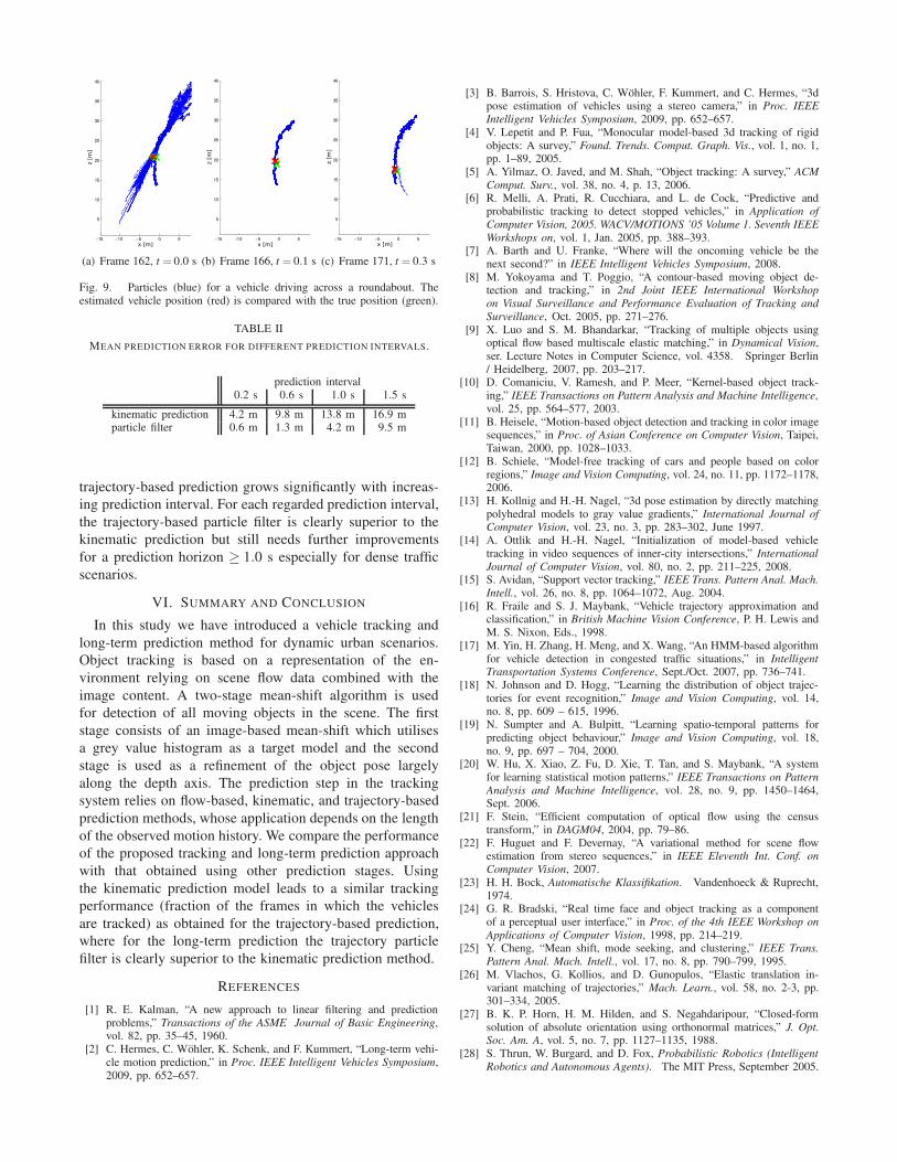
(a) Frame 162, t = 0.0 s (b) Frame 166, t = 0.1 s (c) Frame 171, t = 0.3 s

Fig. 9. Particles (blue) for a vehicle driving across a roundabout. Theestimated vehicle position (red) is compared with the true position (green).

TABLE II

MEAN PREDICTION ERROR FOR DIFFERENT PREDICTION INTERVALS.

prediction interval0.2 s 0.6 s 1.0 s 1.5 s

kinematic prediction 4.2 m 9.8 m 13.8 m 16.9 mparticle filter 0.6 m 1.3 m 4.2 m 9.5 m

trajectory-based prediction grows significantly with increas-

ing prediction interval. For each regarded prediction interval,

the trajectory-based particle filter is clearly superior to the

kinematic prediction but still needs further improvements

for a prediction horizon ≥ 1.0 s especially for dense traffic

scenarios.

VI. SUMMARY AND CONCLUSION

In this study we have introduced a vehicle tracking and

long-term prediction method for dynamic urban scenarios.

Object tracking is based on a representation of the en-

vironment relying on scene flow data combined with the

image content. A two-stage mean-shift algorithm is used

for detection of all moving objects in the scene. The first

stage consists of an image-based mean-shift which utilises

a grey value histogram as a target model and the second

stage is used as a refinement of the object pose largely

along the depth axis. The prediction step in the tracking

system relies on flow-based, kinematic, and trajectory-based

prediction methods, whose application depends on the length

of the observed motion history. We compare the performance

of the proposed tracking and long-term prediction approach

with that obtained using other prediction stages. Using

the kinematic prediction model leads to a similar tracking

performance (fraction of the frames in which the vehicles

are tracked) as obtained for the trajectory-based prediction,

where for the long-term prediction the trajectory particle

filter is clearly superior to the kinematic prediction method.

REFERENCES

[1] R. E. Kalman, “A new approach to linear filtering and predictionproblems,” Transactions of the ASME Journal of Basic Engineering,vol. 82, pp. 35–45, 1960.

[2] C. Hermes, C. Wohler, K. Schenk, and F. Kummert, “Long-term vehi-cle motion prediction,” in Proc. IEEE Intelligent Vehicles Symposium,2009, pp. 652–657.

[3] B. Barrois, S. Hristova, C. Wohler, F. Kummert, and C. Hermes, “3dpose estimation of vehicles using a stereo camera,” in Proc. IEEE

Intelligent Vehicles Symposium, 2009, pp. 652–657.[4] V. Lepetit and P. Fua, “Monocular model-based 3d tracking of rigid

objects: A survey,” Found. Trends. Comput. Graph. Vis., vol. 1, no. 1,pp. 1–89, 2005.

[5] A. Yilmaz, O. Javed, and M. Shah, “Object tracking: A survey,” ACM

Comput. Surv., vol. 38, no. 4, p. 13, 2006.[6] R. Melli, A. Prati, R. Cucchiara, and L. de Cock, “Predictive and

probabilistic tracking to detect stopped vehicles,” in Application of

Computer Vision, 2005. WACV/MOTIONS ’05 Volume 1. Seventh IEEE

Workshops on, vol. 1, Jan. 2005, pp. 388–393.[7] A. Barth and U. Franke, “Where will the oncoming vehicle be the

next second?” in IEEE Intelligent Vehicles Symposium, 2008.[8] M. Yokoyama and T. Poggio, “A contour-based moving object de-

tection and tracking,” in 2nd Joint IEEE International Workshop

on Visual Surveillance and Performance Evaluation of Tracking and

Surveillance, Oct. 2005, pp. 271–276.[9] X. Luo and S. M. Bhandarkar, “Tracking of multiple objects using

optical flow based multiscale elastic matching,” in Dynamical Vision,ser. Lecture Notes in Computer Science, vol. 4358. Springer Berlin/ Heidelberg, 2007, pp. 203–217.

[10] D. Comaniciu, V. Ramesh, and P. Meer, “Kernel-based object track-ing,” IEEE Transactions on Pattern Analysis and Machine Intelligence,vol. 25, pp. 564–577, 2003.

[11] B. Heisele, “Motion-based object detection and tracking in color imagesequences,” in Proc. of Asian Conference on Computer Vision, Taipei,Taiwan, 2000, pp. 1028–1033.

[12] B. Schiele, “Model-free tracking of cars and people based on colorregions,” Image and Vision Computing, vol. 24, no. 11, pp. 1172–1178,2006.

[13] H. Kollnig and H.-H. Nagel, “3d pose estimation by directly matchingpolyhedral models to gray value gradients,” International Journal ofComputer Vision, vol. 23, no. 3, pp. 283–302, June 1997.

[14] A. Ottlik and H.-H. Nagel, “Initialization of model-based vehicletracking in video sequences of inner-city intersections,” International

Journal of Computer Vision, vol. 80, no. 2, pp. 211–225, 2008.[15] S. Avidan, “Support vector tracking,” IEEE Trans. Pattern Anal. Mach.

Intell., vol. 26, no. 8, pp. 1064–1072, Aug. 2004.[16] R. Fraile and S. J. Maybank, “Vehicle trajectory approximation and

classification,” in British Machine Vision Conference, P. H. Lewis andM. S. Nixon, Eds., 1998.

[17] M. Yin, H. Zhang, H. Meng, and X. Wang, “An HMM-based algorithmfor vehicle detection in congested traffic situations,” in IntelligentTransportation Systems Conference, Sept./Oct. 2007, pp. 736–741.

[18] N. Johnson and D. Hogg, “Learning the distribution of object trajec-tories for event recognition,” Image and Vision Computing, vol. 14,no. 8, pp. 609 – 615, 1996.

[19] N. Sumpter and A. Bulpitt, “Learning spatio-temporal patterns forpredicting object behaviour,” Image and Vision Computing, vol. 18,no. 9, pp. 697 – 704, 2000.

[20] W. Hu, X. Xiao, Z. Fu, D. Xie, T. Tan, and S. Maybank, “A systemfor learning statistical motion patterns,” IEEE Transactions on Pattern

Analysis and Machine Intelligence, vol. 28, no. 9, pp. 1450–1464,Sept. 2006.

[21] F. Stein, “Efficient computation of optical flow using the censustransform,” in DAGM04, 2004, pp. 79–86.

[22] F. Huguet and F. Devernay, “A variational method for scene flowestimation from stereo sequences,” in IEEE Eleventh Int. Conf. on

Computer Vision, 2007.[23] H. H. Bock, Automatische Klassifikation. Vandenhoeck & Ruprecht,

1974.[24] G. R. Bradski, “Real time face and object tracking as a component

of a perceptual user interface,” in Proc. of the 4th IEEE Workshop on

Applications of Computer Vision, 1998, pp. 214–219.[25] Y. Cheng, “Mean shift, mode seeking, and clustering,” IEEE Trans.

Pattern Anal. Mach. Intell., vol. 17, no. 8, pp. 790–799, 1995.[26] M. Vlachos, G. Kollios, and D. Gunopulos, “Elastic translation in-

variant matching of trajectories,” Mach. Learn., vol. 58, no. 2-3, pp.301–334, 2005.

[27] B. K. P. Horn, H. M. Hilden, and S. Negahdaripour, “Closed-formsolution of absolute orientation using orthonormal matrices,” J. Opt.Soc. Am. A, vol. 5, no. 7, pp. 1127–1135, 1988.

[28] S. Thrun, W. Burgard, and D. Fox, Probabilistic Robotics (Intelligent

Robotics and Autonomous Agents). The MIT Press, September 2005.