Vegetation Mapping - California State Parks · PDF fileVegetation Mapping Primer California...
54
Vegetation Mapping Primer California Department of Parks and Recreation - Inventory, Monitoring, and Assessment Program Page 1 Vegetation Mapping A Primer For The California State Park System October 2002 Inventory, Monitoring, and Assessment Program Natural Resources Division
Transcript of Vegetation Mapping - California State Parks · PDF fileVegetation Mapping Primer California...

Vegetation Mapping Primer California Department of Parks and Recreation - Inventory, Monitoring, and Assessment Program
Page 1
Vegetation Mapping
A Primer For The California State Park System
October 2002 Inventory, Monitoring, and Assessment Program
Natural Resources Division

Vegetation Mapping Primer California Department of Parks and Recreation - Inventory, Monitoring, and Assessment Program
Page 2
This primer was prepared by Roy A. Woodward (916-651-6940, [email protected]). The following persons performed reviews or provided suggestions regarding this primer: Laurie Archambault, James Barry, Kim Marsden, Cynthia Roye, David Shaari, Jim Suero, and Gary Walter.

Vegetation Mapping Primer California Department of Parks and Recreation - Inventory, Monitoring, and Assessment Program
Page 3
Table of Contents 1. Objectives of Vegetation Mapping ..................................................................................... 5 2. purposes of Vegetation Mapping ....................................................................................... 8
2.1. Classification of Vegetation............................................................................................ 8 2.2. Understanding Spatial Structure of Vegetation Patterns ................................................ 8 2.3. Showing Distribution of a Specific Vegetation Unit ...................................................... 8 2.4. Successional Studies & Trend Assessment ..................................................................... 8 2.5. Predicting Wildlife Use................................................................................................... 9 2.6. Fire Management ............................................................................................................ 9 2.7. Basis for Locating Inventory & Monitoring Sample Points ........................................... 9 2.8. Providing a Framework for Research ............................................................................. 9 2.9. Modeling Effects of Management Actions ................................................................... 10 2.10. Education/Interpretation............................................................................................ 10 2.11. Environmental Compliance....................................................................................... 10 2.12. Habitat Linkages and Acquisition............................................................................. 10
3. Vegetation Characteristics ................................................................................................ 11 3.1. Plant Distribution in California..................................................................................... 11 3.2. Vegetation Patterns ....................................................................................................... 12
3.2.1. ‘Stands’ ................................................................................................................. 12 3.2.2. Potentially Problematic Vegetation Patterns: Zones and Ecotones ..................... 12 3.2.3. Seasonal Changes in Vegetation Pattern............................................................... 13
4. Vegetation Classification Systems .................................................................................. 14 4.1. Manual of California Vegetation (include table & list of types) .................................. 14 4.2. Wildlife Habitat Relationships...................................................................................... 15 4.3. Other Systems ............................................................................................................... 16
5. Types of Vegetation Maps ................................................................................................ 18 5.1. Individual Plant Maps ................................................................................................... 18 5.2. Plant Species Maps ....................................................................................................... 18 5.3. Wildlife Habitat Map .................................................................................................... 19 5.4. Wetlands........................................................................................................................ 20 5.5. Land Use ....................................................................................................................... 22 5.6. Forest Site Map ............................................................................................................. 22 5.7. Soils and Geology ......................................................................................................... 22 5.8. Historical Vegetation .................................................................................................... 23 5.9. Potential Vegetation...................................................................................................... 24 5.10. Existing Vegetation................................................................................................... 24
6. Map Basics.......................................................................................................................... 25 6.1. Scale .............................................................................................................................. 25 6.2. Minimum Mapping Unit ............................................................................................... 25 6.3. Setting Map Boundaries................................................................................................ 26 6.4. Role of Geographic Information Systems..................................................................... 26 6.5. Role of Global Positioning Systems ............................................................................. 27
7. Special Issues ..................................................................................................................... 29 7.1. What about burned or disturbed areas?......................................................................... 29

Vegetation Mapping Primer California Department of Parks and Recreation - Inventory, Monitoring, and Assessment Program
Page 4
7.2. How are exotic species (weeds) classified and mapped?.............................................. 29 7.3. What about landscaped areas and agriculture areas? .................................................... 29 7.4. What about unvegetated or sparsely vegetated areas? .................................................. 30 7.5. What can I do with previously produced vegetation maps for my park? ..................... 30
8. How to Produce a Vegetation Map.................................................................................. 31 8.1. Determine the Area to Map........................................................................................... 31 8.2. Perform Field Reconnaissance...................................................................................... 32 8.3. Map Design Decisions .................................................................................................. 32 8.4. Obtain Aerial Photographs............................................................................................ 33
8.4.1. Black & White, Color, or Infrared ........................................................................ 34 8.4.2. Satellites & Advanced Technologies .................................................................... 34 8.4.3. Digital Orthophoto Quarter Quads........................................................................ 35 8.4.4. Use of Outdated Aerial Photographs .................................................................... 35
8.5. Set Vegetation Classification Rules .............................................................................. 36 8.6. Mapping Technique Selection ...................................................................................... 36
8.6.1. Computer Aided Mapping .................................................................................... 37 8.6.2. Manual Method of Mapping ................................................................................. 39
8.7. Field Check Polygons ................................................................................................... 40 8.7.1. Rapid Vegetation Assessment ............................................................................... 41 8.7.2. Number of field samples to perform..................................................................... 42
8.8. Statistical Analysis of Quantitative Field Data ............................................................. 42 8.9. Reclassify Vegetation & Redraw Polygons .................................................................. 43 8.10. Produce Final Vegetation Map ................................................................................. 43
9. Glossary............................................................................................................................... 44 References and Links.................................................................................................................... 46 Table 4-1 A hierarchal vegetation classification system 47 Table 4-2 California Wildlife Habitat Relationships system habitat types 48 Table 5-1 Crosswalk of various vegetation classification systems 51 Table 6-1 Map scale comparison table 52 Figure 8-1 Vegetation map procedure flow chart 53 Attachment 8-1 CNPS Vegetation Rapid Assessment Protocol 54

Vegetation Mapping Primer California Department of Parks and Recreation - Inventory, Monitoring, and Assessment Program
Page 5
1. OBJECTIVES OF VEGETATION MAPPING This primer is intended as an introduction to vegetation mapping for ecologists and planners working in the California State Park System. It can serve as a ‘how to’ manual for those who will conduct vegetation mapping projects, but also is intended as an introduction to the topic for those who may never construct a vegetation map but who want to become familiar with the principles. Certain standards are presented in this primer; however, the art and science of vegetation mapping is ever advancing and improved mapping criteria will be distributed as they become available. It is seldom practicable to map every individual plant growing in a park, though on occasion this is done for rare or significant species such as endangered species or old growth trees. Instead of mapping every individual plant it is usually necessary to combine or ‘classify’ the plants into groups (for vegetation classification and mapping purposes these groups are called ‘stands’) based on the most dominant species present (this may be one or many species.) Dominance is based on the amount of land surface covered by plant stems or canopy and/or the total number of individuals of a plant species. The justification for combining plant species into consistent stands is based on the observation that plant species do not occur randomly across the landscape, but naturally occur in stands based on environmental factors such as soil type or amount of precipitation. A stand is a group of plant species wherein the dominant plant species are similar in size (height, diameter, cover) and abundance (density, basal area, number of canopy layers.) Stands of vegetation can be designated by names or symbols (referred to as ‘vegetation types’) and presented on a map in a consistent and logical fashion; this is the basis for vegetation mapping. Vegetation maps generally present a bird’s-eye-view of stands of plant species as they occur across the landscape, somewhat akin to a portrait of the landscape at that particular time. Vegetation maps typically consider only terrestrial vascular plants (trees, shrubs, forbs, and grasses) and do not attempt to map mosses, liverworts, lichens, or purely aquatic plants including algae/kelp, though in some instances these elements may be mapped. Stands of vegetation generally form a mosaic of types across the landscape, and it is possible to delineate individual stands of vegetation on a base map, such as a U.S.G.S. topographic quadrangle map, by drawing a line around the boundary of each vegetation stand. Individual vegetation stands are identified and mapped by visual differences of color, texture, or size based on examination of aerial photographs. The observed differences between stands visible on aerial photographs are usually caused by changes in plant species composition, height of the vegetation, and/or amount of plant cover. The boundary lines around separate stands of vegetation form a group of irregularly shaped polygons, with each polygon containing a different stand of vegetation. Some polygons may be small and others quite large depending on how common various vegetation types are in the area. Also, some vegetation types may occur as a single polygon in one part of the map, while other vegetation types have many polygons scattered across the map. Section 6 discusses methods for deciding

Vegetation Mapping Primer California Department of Parks and Recreation - Inventory, Monitoring, and Assessment Program
Page 6
where to draw the polygon boundary lines and how small of an area to consider when defining polygons. Polygons of vegetation stands are almost never square or round, but their outline is usually very uneven and after vegetation polygons are drawn on a base map they often look like pieces of a jigsaw puzzle. A vegetation map consists of polygons of stands of plants, with each polygon designated by a unique color or symbol that is linked to a legend or description of the specific vegetation type. Other map elements, such as roads, streams, and park boundaries are often added as reference points on the map. Two major questions immediately arise when designing a vegeta tion map, (1) What system should I use to combine or classify the plant species into stands? and, (2) What size of area should be included in each stand?, or generally best considered as, ‘How small of an area do I want my smallest stand of plants to encompass?”. Decision rules must be followed to decide how various stands of plants, especially stands with mixtures of many species, will be named (classified.) There are different methods of classifying vegetation, and most methods are hierarchal, that is they range from general types of vegetation (‘forest’) to very specific classifications (‘Monterey pine series’.)1 To be meaningful the vegetation should be classified before it is mapped, and there is a discussion of vegetation classification in Section 4 of this primer. Mapping methods and tools are also discussed in this primer (Section 6.) Decisions must be made early in the mapping process regarding map scale, minimum mapping units, and what you want the final product to look like. Vegetation maps can show floristic (what taxa are present) and physiognomic (the ‘appearance’ of the vegetation, i.e., its life form and architecture) information in a manner useful for resource assessment. The types of plants present in a park, their abundance, and their distribution can be clearly presented by a well-constructed vegetation map. To be most useful vegetation maps should be produced at a scale and resolution that easily conveys the intended information. Also, the map should contain a key of the names of the vegetation types shown on the map, and the best maps are accompanied by tables of quantitative vegetation data, such as cover and density and size, obtained from sampling the mapped stands in the field to collect quantitative data about each stand. This primer discusses the considerations of these various decisions and proposes standards for designing vegetation maps for state parks. In some cases vegetation maps may be used as a tool for assessing wildlife habitat (i.e. to determine what wildlife species are present and/or to what uses animals might be putting an area); however, animal distribution has been shown to vary greatly based on both the structural variables in the landscape (e.g., number of snag trees, sources of drinking water, amount of debris on the forest floor) and not solely on the plant species
1 Hierarchy systems commonly used in California follow the Federal Geographic Data Committee guidelines. This hierarchy, from largest to smallest, contains the following categories: Order, Class, Subclass, Group, Formation, Alliance (also called a Series), and Community Association (also called Plant Community.)

Vegetation Mapping Primer California Department of Parks and Recreation - Inventory, Monitoring, and Assessment Program
Page 7
composition. Therefore, an effective ‘cross-walk’ between vegetation maps, which generally consider only limited structural components, and wildlife habitat does not exist for many wildlife species. Also, areas of isolated wildlife habitat, especially in small parks with no or tenuous connections to other habitat areas, may not be inhabited by all of the wildlife species that might be expected to occur there even if all of the correct habitat elements appear to be present because the wildlife may have been extirpated for some unknown reason and have been unable to reinhabit the area. In September 2000 the Department of Parks and Recreation signed a Memorandum of Understanding with other state and federal agencies regarding consistent standards for vegetation mapping in California.2 It benefits the Department to cooperate with other agencies when conducting vegetation-mapping projects, and to ensure that data is collected uniformly and can be electronically shared. This primer is designed to be consistent with this MOU.
2 See http://ceres.ca.gov/biodiversity/vegmou.html

Vegetation Mapping Primer California Department of Parks and Recreation - Inventory, Monitoring, and Assessment Program
Page 8
2. PURPOSES OF VEGETATION MAPPING The following are brief explanations of the major uses of vegetation maps for State Park System units.
2.1. Classification of Vegetation A vegetation map serves as an easy way to portray the existing status of vegetation across the park landscape. Some groupings of plants, such as ‘forest’ or ‘grassland’, are obvious, but most plant associations occur more subtly yet they have a profound influence on the environment and character of the park. A vegetation map is one of the most useful ways to obtain a ‘big picture’ view of the natural environment of a park, and is the basis for any rapid assessment of the condition of a park.
2.2. Understanding Spatial Structure of Vegetation Patterns
Plants and groupings of plants do not occur randomly over the landscape. Vegetation maps provide a means of studying where plant groupings occur, and are a starting point for determining what factors have produced the existing vegetation spatial structure. Studying vegetation can serve as a surrogate for measuring other environmental factors that may be more difficult to assess, such as climate or soil/geology. Also, the rarity or local significance of stands of vegetation can be evaluated by analysis of vegetation maps.
2.3. Showing Distribution of a Specific Vegetation Unit A vegetation map serves as a tool to locate specific vegetation types (groupings of plants) in a park. These groupings may be significant because they contain noteworthy plants, such as old growth trees, or because the groupings of plants provide wildlife habitat or enhance the visitor’s experience. This is important when planning restoration/revegetation projects and understanding where significant stands of vegetation occur that should be protected from disturbance.
2.4. Successional Studies & Trend Assessment Vegetation maps created at different times can be compared to assess the status and trend of the condition of vegetation, and by association wildlife habitat and wildlife. Adaptive management of parklands can be based on plant changes detected on vegetation maps constructed at different times. Fire history of the park and outbreaks of disease or pests can be studied by comparison of vegetation maps over time.

Vegetation Mapping Primer California Department of Parks and Recreation - Inventory, Monitoring, and Assessment Program
Page 9
2.5. Predicting Wildlife Use The species of wildlife that occur in parks, and the types of uses they make of a park, such as feeding or breeding, is generally correlated with vegetation type. Mapping vegetation assists wildlife biologists to predict what wildlife species may be present, and where the most critical areas of habitat exist.
2.6. Fire Management
Vegetation maps can be used to help model fuels that in conjunction with slope, aspect and weather information can be input into models to predict the rate and direction of spread of wildfires. Also, public and firefighter safety can be assessed by examination of vegetation maps before and during wildfires. Planning prescribed burn priorities to treat the most critical vegetation types, and protect the most sensitive areas, requires a vegetation map. Vegetation maps can also be useful to track post-fire recovery of burned areas in relation to non-burned areas.
2.7. Basis for Locating Inventory & Monitoring Sample Points It is impossible to measure and count each natural feature in a park to assess the condition of the resources; therefore, a subsample of the total must be selected for measurement. Subsamples are selected based on statistical principles that define how much data must be collected in order to obtain a given amount of confidence in the results. An important element of scientific studies is to increase efficiency of inventory and monitoring by stratifying the sampling area based on existing environmental conditions, such as topography, soil type, or vegetation type. A vegetation map is an important tool for selecting sampling points for inventory, monitoring, and designing scientific studies to assess park resources.
2.8. Providing a Framework for Research
Under natural conditions plants are generally distributed according to rainfall, temperature, aspect/elevation, and soil/geology type. Also, past land uses and barriers to plant dispersal is expressed in the existing flora of an area. Moreover, wildlife is commonly associated with certain vegetation types. A vegetation map efficiently integrates all of these factors by presenting a picture of the park showing the areas of occurrence of the most dominant plant species, and thereby providing information about abiotic factors and wildlife as well. Researchers seeking to answer questions about the environment inside of a park may rely heavily on vegetation maps to indicate existing and past conditions to begin to identify causal relationships.

Vegetation Mapping Primer California Department of Parks and Recreation - Inventory, Monitoring, and Assessment Program
Page 10
2.9. Modeling Effects of Management Actions A key element of park planning includes an understanding of what vegetation communities are present, and how various park management actions may affect the vegetation, which allows for specific planning regarding the place and time of year that many recreational activities can best take place to have the minimum impact on natural resources. Several park management issues can be effectively addressed by reference to vegetation maps including planning locations of facilities, locating rare species associated with a particular vegetation type, or modeling occurrences of plants or wildlife based on habitat needs. By understanding vegetation patterns and natural selection it becomes possible to better understand the results of management decisions. For example, the successfulness of locating and constructing trails away from sensitive resources, such as wetlands or meadows, can be best determined by understanding how vegetation in the entire affected area has responded.
2.10. Education/Interpretation Informing park visitors about locations of park resources is much more efficient when vegetation maps are available for a park. For example, birders can quickly determine where the best areas to practice their sport occur after examining a vegetation map. Interpretation of cultural and historical resources is also aided when reference can be made to vegetation maps. An added value of vegetation mapping is helping the public and park decision makers see the ‘big picture’ of what resources are available in a park and how significant they are on a regional scale. Also, a more complete plant species list for a park is generally developed during field-checking when a vegetation map is created for a park.
2.11. Environmental Compliance A vegetation map can be used to assist completion of environmental compliance documents, such as during the CEQA (California Environmental Quality Act) process, by effectively giving an overview of existing park conditions, and helping to put things in perspective when describing potential affects of proposed park management activities.
2.12. Habitat Linkages and Acquisition
Ecosystem models have shown that corridors providing linkages that allow for genetic exchange between isolated park units are necessary for long-term viability of many wildlife and plant populations. Any assessment for determining if sufficient linkages exist or potentially exist, and what areas should have highest priority for acquisition requires a vegetation assessment. A park-wide vegetation map that includes surrounding areas is a useful tool for determining the importance of any park acquisition.

Vegetation Mapping Primer California Department of Parks and Recreation - Inventory, Monitoring, and Assessment Program
Page 11
3. VEGETATION CHARACTERISTICS This section provides a brief discussion of vegetation patterns commonly observed in California.
3.1. Plant Distribution in California California has approximately 6,300 native vascular plant species, and hundreds of species of non-native plants, distributed on over 104,000,000 acres (165,000 square miles.) Some species are very restricted in range with an entire population consisting of only a few individuals occupying a few acres, whereas other species can be found in almost every county. Annual species are herbaceous and many annual species germinate, flower, and die within a few short weeks, with some species laying dormant in the soil as seed for many years until a soil disturbance or adequate rainfall stimulates germination. Perennial species live for more than one year following germination or sprouting, including some individual forest trees and desert shrubs known to be thousands of years old. These thousands of species grow where they do because of complex ecological factors, sometimes influenced by humans, including rainfall, temperature, soil type and hydrology, geology, land disturbance/erosion, fire, barriers to movement, light/sunshine, pests, disease, pollinators, fog, salt air, grazing/herbivory, and competition with one another. Year-to-year changes in the size of individual plants, especially annual species, and thus the area of ground covered by these species is largely caused by variable rainfall; regular recurring rainfall cycles in California caused by El Niño and La Niña effects are well documented. The most dramatic changes occur in the deserts, where areas may lay barren for many years, but become totally covered by vegetation a short time after a rainstorm. Wildfire, logging, or livestock grazing can also change the species composition and/or cover of vegetation year-to-year. Other factors, such as the introduction of a new weed species or natural succession, may slowly cause the vegetation of an area to change from one type to another. Of course, an acute impact, such as development, causes permanent conversion from natural vegetation to non-vegetated, agricultural, or landscaped types. Vegetation classification and mapping is largely concerned with identifying the types of plants that dominate an area at a given moment in time (usually the moment when an aerial photograph is taken or a field check is performed.) Therefore, the species of plants and their number and size are what determine the vegetation type of an area.

Vegetation Mapping Primer California Department of Parks and Recreation - Inventory, Monitoring, and Assessment Program
Page 12
3.2. Vegetation Patterns
3.2.1. ‘Stands’
Vegetation classification and mapping are possible because plant species occur in groups or ‘stands’ of plants wherein each individual species is responding to similar ecological factors in a given area. Stands are variable in size and shape and can be less than an acre or cover thousands of continuous acres.3 Many types of stands often occur in close proximity to each other in mosaic patterns based on ecological factors and stand history. Stands with similar plant species and site histories will be classified and mapped alike. Individual plant species can have broad adaptations to ecological factors, so that two distinct vegetation stands dominated by two quite different species may have a third species that readily occurs with both of them as a co-dominant. This situation is easily mapable as long as the vegetation classification system is robust enough to allow for such variability.
3.2.2. Potentially Problematic Vegetation Patterns: Zones and Ecotones
A common vegetation pattern observed in nature is a zone or belt. Zones typically form whenever plant species are responding to an environmental gradient and may be massive in scale, such as the bands of different conifer species encountered as elevation increases up a mountain range, or be micro in scale such as rings of flowering species that can be seen blooming around individual vernal pools in springtime. An example of a vegetation belt is riparian vegetation that occurs along the banks of waterbodies, or a band of non-shade tolerant shrub or tree species that sometimes occur at the margins between forests and grasslands. Often the ecological factors causing the gradient where different plant species grow in zones or belts are not completely known. It is not difficult to distinguish forest from grassland, but deciding exactly where the edge of the forest begins and where the edge of the grassland ends can be a more difficult decision because these transitions often occur very gradua lly, or perhaps the area is a true savannah with a climax mixture of trees and grasses and there is no true edge. The transition area between different vegetation types is referred to as an ‘ecotone’. Ecotones may be so narrow they do not affect vegetation classification because the boundary between two vegetation types is abrupt, but if the ecotone is broad and species changes occur gradually vegetation classification becomes more difficult. If ecotones are large enough they may be classified as a separate distinct vegetation type, or described and mapped as a mixture of two vegetation types, for example California Annual Grassland Series-Valley Oak Series.
3 Note: Stand size can be observed and measured on the landscape and is not the same as ‘minimum mapping unit’ (MMU), which is a decision by the designer of a vegetation map based on several factors.
Vegetation Mapping Primer California Department of Parks and Recreation - Inventory, Monitoring, and Assessment Program
Page 13
Classification of zones and ecotones is one of the most highly subjective tasks when classifying and mapping vegetation because the vegetation types are not discrete and easily defined. In most cases only very detailed research projects would attempt to classify and map micro-scale vegetation zones, and vegetation classification systems typically do not deal with vegetation at this scale (i.e., areas less than 0.5 acres in size.) Occasional outliers, such as an occasional forest tree growing in an otherwise grassland area, are best ignored and the area can be consistently mapped as ‘grassland’ if that is what truly dominates the area. Small-scale vegetation mapping always promotes generalizations because there is just too much information to fit into small mapping units. If stands of vegetation can be identified and delineated at a large enough scale, for example the Alliance level, then classification and mapping can generally proceed without much fretting about how to combine diverse vegetation types.
3.2.3. Seasonal Changes in Vegetation Pattern Seasonal changes of vegetation are another complicating factor of vegetation classification and mapping in some vegetation types, especially those dominated by annual species. Obviously, the ideal time to classify vegetation is when leaves/foliage are present during the peak growing season, and aerial photographs taken at these times of year should be used for classification and mapping. However, some vegetation types do not have a single peak growing period because the many different plant species that grow in some area are responding to short-term rainfall events, such as in the desert, or successive waves of plants grow and dominate sites for short periods of times over the growing season, such as annual grassland areas that may have a phase of domination by wildflowers, then grasses, then tarweeds over the course of several months. The best thing to do is to classify and map these types according to the dominant species encountered at the time of the classification effort and be sure the written vegetation descriptions that accompany the vegetation map include an explanation of the changing nature of the area. On some occasions it may be desirable to map only perennial vegetation, so the effort would use air photos taken when annuals were dormant, and field checking might ignore the annual vegetation layer altogether.

Vegetation Mapping Primer California Department of Parks and Recreation - Inventory, Monitoring, and Assessment Program
Page 14
4. VEGETATION CLASSIFICATION SYSTEMS In California the standard system that is used in most vegetation classification and mapping situations is the Manual of California Vegetation (MCV.) The following section briefly describes the MCV and some other vegetation classification systems that might be encountered in California.
4.1. Manual of California Vegetation (include table & list of types)
The first edition of the Manual of California Vegetation (MCV4) was published in 1995 authored by John Sawyer, a Professor at CSU Humboldt, and Dr. Todd Keeler-Wolf, a vegetation ecologist with the California Department of Fish and Game. A committee of professional plant ecologists chaired by Professor Michael Barbour, UC Davis, and organized by the California Native Plant Society developed the classification system described in the MCV over several years. The MCV contains taxonomic keys to vegetation types based on species composition, written descriptions of each vegetation type with extensive citations regarding each type, and representative photographs of many vegetation types. The MCV was designed to be consistent with on-going national vegetation classification efforts.5 The MCV vegetation classification system follows a hierarchy that is floristically based (i.e., names of vegetation types are derived from the names of the prominent plant species rather than the geographic location or physiognomic structure of stands), and gives fine-scale descriptions of vegetation types at the ‘series’ (alliance) and ‘association’ (plant community) levels (see Table 4-1.)6 Examples of vegetation alliances (also called ‘series’) used in the MCV are ‘fourwing saltbush series’, ‘purple needlegrass series’, ‘red fir series’, and ‘tecate cypress stands’. The vegetation series and associations described in the system are from published field efforts by the authors and many others, in addition to thousands of hours of field surveys throughout California to visit and describe the existing vegetation of the state and understand where different plant species grow and how these species are associated with other plant species. A hallmark of the MCV vegetation classification system is reliance on quantitative sampling of vegetation stands in the field to establish species composition and cover values. The MCV describes a technique for quantifying vegetation cover using plots and plotless methods. Recent refinements of the quantitative method have resulted in the California Native Plant Society – Vegetation Rapid Assessment Protocol.7
4 See http://davisherb.ucdavis.edu/CNPSActiveServer/Index.html or http://www.cnps.org/vegetation/vegmanual.htm 5 See http://esa.sdsc.edu/vegwebpg.htm 6 In a broad sense any assemblage of vegetation can be termed a ‘plant community’, and the term plant community is often used by ecologists in general discussions to refer to different vegetation stands at different levels of the vegetation classification hierarchy. For purposes of this primer ‘plant community’ is used solely to refer to vegetation stands classified at the Association level. 7 For a copy of the protocol and field data form see http://www.cnps.org/vegetation/protocol.htm

Vegetation Mapping Primer California Department of Parks and Recreation - Inventory, Monitoring, and Assessment Program
Page 15
The 1995 edition of the MCV describes 275 different vegetation types, and discusses the existence of other problematic categories called ‘unique stands’, ‘habitats’, and ‘vernal pools’. These 275 types define approximately 240 different ‘alliances’,8 and 625 ‘associations’.9 Also, if ecologists discover new vegetation types not described in the MCV classification system these new types can be named (and mapped) based on their dominant species. If new vegetation types are described, information about the site, along with plant species composition and cover values, should be submitted to the California Department of Fish and Game and/or California Native Plant Society for possible inclusion in future editions of the MCV. The California Department of Fish and Game and California Native Plant Society maintain a computer database, named California Vegetation Information System (CVIS), of quantitative data collected for any vegetation type in California, and they encourage submission of any such data for inclusion in this system.10 A second edition of the MCV that includes the latest vegetation type descriptions and expands the effort to clarify the problematic categories is anticipated for publication in 2003, and is expected to more than double the number of different vegetation types in the state based largely on work in recent years in the deserts. Dr. Keeler-Wolf has estimated that at least 2,000 plant associations may eventually be described for California.
4.2. Wildlife Habitat Relationships According to the California Department of Fish and Game the California Wildlife Habitat Relationships (CWHR)11 system is “a comprehensive information system for California wildlife that describes, models, and predicts: (1) habitat relationships and requirements; (2) management status; (3) geographic distribution; (4) life history; and (5) responses to habitat changes of wildlife species in the system”. Models have been developed in the CWHR for over 675 of the more than 930 known vertebrate wildlife species in California. The CWHR was developed by an interagency task group of wildlife biologists with the first edition of A Guide to Wildlife Habitats of California, edited by Kenneth Mayer and William Laudens layer, published in 1988; subsequent versions of the database portion of the system have been released on computer disk as they were developed with the most recent being Version 7 released in 1999 (Version 8 is expected for release in late 2002.)
8 As defined by Dr. Todd Keeler-Wolf an alliance is defined as “a uniform group of associations which share one or more diagnostic species that are usually found in the uppermost layer of the vegetation.” An example of an alliance is ‘coast redwood forest type’. 9 As defined by Dr. Todd Keeler-Wolf an association is “the most basic unit in the classification system – defined as a uniform group of vegetation stands that share one or more diagnostic species in the overstory and understory. The species and structure of each association occur repeatably across the landscape and are generally found in similar environmental conditions.” An example of an association is ‘coast redwood/swordfern type’. 10 To submit data to CVIS contact vegetation ecologist Julie Evens ([email protected]) or Todd Keeler-Wolf ([email protected]). 11 See http://www.dfg.ca.gov/whdab/html/cwhr.html

Vegetation Mapping Primer California Department of Parks and Recreation - Inventory, Monitoring, and Assessment Program
Page 16
The CWHR describes 59 different habitat types in California (see Table 4-2) that are largely based on vegetation type, although CDFG points out that the CWHR habitat types are “not a vegetation classification system per se”. Unfortunately, there is not a complete correspondence between the CWHR and the MCV, so that one area may be named two different ways. This is somewhat obvious considering the MCV has over 275 types and the CWHR only 59 types, but the problem is the MCV types cannot be rolled-up into the 59 CWHR types consistently. It is possible to classify park areas according to CWHR type and map these areas, and in some cases this may be done; however, for most park purposes it is more useful to classify vegetation according to the MCV.
4.3. Other Systems Several other vegetation classification systems have been used in California in the past, and it might be useful to know how these may have been applied to produce earlier vegetation maps for some parks. The following discusses only the most prominent of these systems, though vegetation ecologists beginning in the early 1900’s have developed many different systems. The major floras (reference books containing taxonomic keys used to consistently identify p lant species) used in California for the past forty years have been A California Flora (Munz 1959) and The Jepson Manual (Hickman 1993.) Each of these floras contains a discussion of plant habitats, particularly as they relate to plant distribution, e.g., a species might be described as occurring in “sagebrush” or “serpentine”, and maps were provided with The Jepson Manual showing California floristic provinces. Neither of these manuals was intended as a guide for classifying vegetation, but they provided general names of plant associations to help persons using the manuals to more easily identify individual plant species by knowing which species commonly occur together. There has been no known attempt to map vegetation based on the descriptions in either of these manuals. The first attempts to map the entire vegetation of California were done by A.E. Wieslander in the 1930s. Wieslander had been a student of Willis Linn Jepson at UC Berkeley, and Professor Jepson had initiated vegetation mapping projects as early as 1914 (Jepson, Beidleman, and Ertter 2000.) The first widely distributed vegetation map that mapped ‘natural vegetation’, titled, “Natural Vegetation of California”, was produced by A. W. Küchler in 1977 and published in Terrestrial Vegetation of California (Barbour and Major 1977.) The map included with the book was printed 40” X 48” and is notable because it can still be found hanging on the walls of many ecologist’s offices in California. The map was done at 1:1,000,000 scale and contained 54 vegetation types for the entire state, which are described in Barbour’s and Major’s book.
Vegetation Mapping Primer California Department of Parks and Recreation - Inventory, Monitoring, and Assessment Program
Page 17
A system developed by the California Department of Fish and Game in 1986 for the California Natural Diversity Data Base12 and derived from earlier work by Cheatham and Haller (1975), and often referred to as the Holland system (after its chief author Dr. Robert Holland), was never published but gained widespread use. The system does not have consistent criteria for naming or identifying vegetation types so that some types are named after the most prominent plant species, while other names may be based on the location of the vegetation type or the geologic substrate or soil type it occurs on. Many park inventories completed in the late 1980s and early 1990s describe vegetation based on the Holland system. The Holland system served as the chief forerunner to development of the MCV. California Senior State Park Resource Ecologist Dr. James Barry also developed a vegetation classification system in the mid-1980s based on his wide breadth of experience in the State Park System. This system was never published outside of the Department of Parks and Recreation and never widely adopted for use by the Department. Dr. Barry still infrequently updates the system with the most recent version being Version 4.6, October 2000. Copies of this system can be obtained directly from Dr. Barry (California Department of Parks and Recreation, P.O. 942896, Sacramento, CA 94296-0001.) At some levels Dr. Barry’s system and the MCV have converged and there is consistency when using either system to classify/map vegetation. Several federal agencies and the California Department of Forestry and Fire Protection Fire and Resources Assessment Program (FRAP)13 have also developed vegetation mapping schemes principally aimed at management of forest and rangelands. The FRAP has produced maps of plant species groupings that include tree size and tree canopy closure with a minimum mapping unit of 2.5 acres. These systems do not generally have broad application for state parks. The National Vegetation Classification system, and the Federal Geographic Data Committee have developed mapping standards that the MCV seeks to follow, so use of the MCV should result in uniformity with these efforts.
12 See http://www.dfg.ca.gov/whdab/html/cnddb.html 13 See http://frap.cdf.ca.gov/

Vegetation Mapping Primer California Department of Parks and Recreation - Inventory, Monitoring, and Assessment Program
Page 18
5. TYPES OF VEGETATION MAPS Various types of vegetation maps are described here, along with their uses and some considerations that affect development of these maps. An interesting list of vegetation and plant distribution maps with links to those maps has been compiled by Claire Englander and Philip Hoehn at UC Berkeley and is available online at http://www.lib.berkeley.edu/EART/vegmaps3.html#noamer.
5.1. Individual Plant Maps In some instances maps have been developed that show the locations of all individuals of a particular plant species. Technically this is not a ‘vegetation’ map but an ‘individual plant’ map. These maps have typically been developed for old growth or significant forest stands (such as Sierra redwood or Monterey pine), for endangered species, or for special areas of parks such as around historical structures. Often these maps show the size of individual tree canopies or basal areas as well as plant locations. These maps are useful for assessing changes in plant density or cover over time, studying associations of the species with the environmental setting such as soil type or aspect, or for planning specific projects inside of vegetation stands that require avoidance of individual plants. There is no need to classify the vegetation when mapping individual plants, but some decisions are still required, such as how to map seedlings or standing dead trees, that will be based on the intended uses of the map. Mapping individual plants is time consuming and not practical for all species or for widespread rare species in large parks. No particular guidance is suggested at this time for mapping individual species other than it is recommend that maps be based on standard Department of Parks and Recreation base maps using existing Department of Parks and Recreation GIS standards.14
5.2. Plant Species Maps In some cases, especially for special status species such as exotic plants (weeds), species maps may be created that show the general distribution of a species in a park and some portrayal of the extent of the species, such as cover or density.15 Unlike a map for an ‘individual plant’ each individual plant is not mapped for a species map, but groups of the plant are classified into polygons or zones depending upon the changing cover or density of the species. This type of map has limited use as a vegetation map because the distributions of only one or a few species are mapped, and the associations of these species with other species are ignored. However, these maps 14 See http://naturalresources.team.parks.ca.gov/IMAP/ 15 ‘Cover’, usually presented as a percentage, refers to the aerial extent of foliage and stems and is a common measure of plant dominance. ‘Density’, usually presented as the number of plants per given area (e.g., 100/acre), refers to the actual number of plants per given area and is a measure of plant abundance. The species with the highest ‘density’ is not always the species with the highest ‘cover’, so when selecting one or the other it is important to explain why it was chosen as an indicator.

Vegetation Mapping Primer California Department of Parks and Recreation - Inventory, Monitoring, and Assessment Program
Page 19
can be useful for designing and tracking progress of weed-control programs or revegetation success. At this time there are not commonly accepted mapping classification schemes for exotic species, i.e., names or designations for zones of cover or density are not standardized and can be chosen arbitrarily by the person creating the map. This can be a problem if the zones are not quantified, because areas designated as ‘high’ zones for cover on one map cannot be related to ‘high’ zones on other maps that may have used a different set of criteria for determining what is ‘high’. If plant density or cover is quantified, then this data can be consistently classified into zones that reflect this data and are easily mapped, for example: Zone 1 = 0-10% cover, Zone 2 = 11-25% cover, and so forth. An effort is underway to develop mapping standards for weeds by the National Association of Weed Management Agencies. An issue when mapping some exotic species is their patchy occurrence; i.e., a species is not widespread over the park, but where it occurs it is in very dense stands. Mapping these stands often requires a relatively large-scale map with high resolution because the stands are often quite small but ecologically significant because of the high-impact they have on that spot and their potential to spread seed/propagules to other areas. Processes for mapping exotics and other species is under development for State Parks. On-going programs can utilize existing park base maps and GIS technology, and newly developed classification schemes and mapping processes will be made available as they are developed.
5.3. Wildlife Habitat Map The California Interagency Wildlife Task Group and the California Department of Fish and Game have developed a wildlife habitat classification scheme called the California Wildlife Habitat Relationships System (CWHR).16 This system has collected habitat data for over 675 species of wildlife in California and identified 59 different large-scale habitat types in the state that are generally based on dominant plant species (see Table 4-2.) In general, the CWHR should not be used to classify vegetation in areas smaller than 40 acres because it violates the rules of the CWHR model. It is possible to compare these 59 habitat types with other vegetation classification systems and discover where the systems overlap or are different, and in this manner it would be possible to produce a ‘cross-walk’ between two different classification systems so that different categories of classification units could be compared. Existing vegetation classification systems are generally hierarchal, and can match quite well with the CWHR at high or mid levels of classification (e.g., the CWHR habitat type ‘Annual Grassland’ corresponds well with the California Manual of Vegetation (MCV) ‘California
16 See: http://www.dfg.ca.gov/whdab/html/habitats.html and http://www.dfg.ca.gov/whdab/html/cwhr.html
Vegetation Mapping Primer California Department of Parks and Recreation - Inventory, Monitoring, and Assessment Program
Page 20
Annual Grassland Series’.) However, at the lower levels, i.e., finest scale, of classification most vegetation classification systems use many more categories, e.g., the MCV has 275 different types of classifications for vegetation compared to the 59 habitat types for CWHR. It is not always possible to role-up the more finely classified categories of a system such as MCV into the larger habitat types of the CWHR because some of the finer categories could potentially be placed in more than one of the larger classes (e.g., the MCV has a single classification named ‘Blue Oak Series’, while the CWHR has two categories named ‘Blue Oak Woodland’ and ‘Blue Oak-Foothill Pine’. Placing a stand into the single MCV ‘blue oak’ category and mapping it as such makes it impossible to determine where the stand belongs under the CWHR classification scheme unless there is more extensive quantitative data available describing the stand.) Also, vegetation classification considers all of the species in a stand before determining what species dominate, based on cover or density, whereas the CWHR has fixed categories for dominant species so any type of vegetation must be fit into one of the existing 59 habitat types rather than creating a new vegetation type (the MCV allows creation of newly discovered vegetation types if they can be adequately described by quantitative assessments of the species present.) Additionally, without quantitative data of plant cover and density a subjective decision must be made about how to place a particular stand in a classification category so there can be great ambiguity among different wildlife habitat and vegetation classification schemes. Whereas vegetation maps are largely concerned with the distribution and extent of cover of living plants, wildlife habitat classifications consider other environmental elements including soils, caves, cliffs, presence of forage (e.g., leaves, fruit, flowers), trees with loose bark and cavities, nearness and types of waterbodies, manmade elements (e.g., nest boxes, transmission lines, agricultural fields), and dead and decaying vegetation such as snags, brush piles, and downed logs. Only at the higher levels of classification does it appear possible to have a close link between vegetation types and precise wildlife habitat types (see Table 5-1.)
5.4. Wetlands The U.S. Army Corps of Engineers 1987 Wetlands Delineation Manual defines a wetland as:
“Those areas that are inundated or saturated by surface or ground water at a frequency and duration sufficient to support, and that under normal circumstances do support, a prevalence of vegetation typically adapted for life in saturated soil conditions. Wetlands generally include swamps, marshes, bogs, and similar areas.”
Determination of whether a given area is a wetland is based upon the characteristics of three components, viz. (1) hydrology, (2) soil, and (3) plant species. Standard wetland delineation performed using the U.S. Army Corps of Engineers 1987 Wetlands Delineation Manual considers the presence of certain plant species that have been

Vegetation Mapping Primer California Department of Parks and Recreation - Inventory, Monitoring, and Assessment Program
Page 21
designated as ‘wetland indicator species’, and lists of these species and their value in determining if an area is a wetland have been prepared for each individual state.17 At this time there are no designated ‘wetland vegetation types’, but only wetland indicator plant species for delineating a wetland. Some vegetation types composed largely of wetland indicator plant species appear to occur only in areas that consistently have hydrological conditions and soil types that would cause the area to be delineated as a wetland. Large-scale wetlands mapping efforts take advantage of this fact by often relying solely on aerial or satellite photographs to determine what areas are wetlands based on the key characteristic of cover by certain dominant plant species. For example, an area dominated by cattail (Typha sp.) or bulrush (Scirpus sp.) would almost always be automatically classified as a wetland. One of the large wetland mapping efforts for the entire United States is the National Wetlands Inventory project of the U.S. Fish & Wildlife Service.18 Also, hydrologic maps have been created by government agencies for various purposes, and some of these may contain information about vegetation and plant species. Therefore, maps of wetlands may also serve as maps of certain plant species, though in many cases the total vegetation of the area has not been classified using any widely recognized classification system. Wetland maps often name the vegetation based on only a few dominant wetland indicator species and, because they are constructed with a different aim in mind they do not necessarily follow vegetation classification rules used by vegetation classification systems such as the Manual of California Vegetation, and the wetlands mapping scheme may not be used interchangeably with other vegetation maps. An issue associated with wetland mapping is riparian area mapping. The term ‘riparian’ is used in different ways in California and can refer to the large tree-dominated stands of oak, walnut, sycamore, maple, willow, and cottonwood that line many of the state’s streams (or at least that lined them at one time), it can refer to any vegetation that occurs next to the shoreline of a waterbody (stream or lake), or it is used to refer to a category of wildlife habitat that encompasses many vegetation types. The distance that a riparian area extends away from the edge of a wate rbody is quite variable, based on topography, soil, and hydrology, so there is no firm rule for determining the size of a riparian area. In most cases, overlaying a waterbody map with a vegetation map (constructed using a standard vegetation classification system) can suffice as a ‘riparian map’ with the potential user of these two combined maps deciding where they want the riparian area to begin and end.
17 For a list of wetland indicator plants see http://www.nwi.fws.gov/bha/ 18 See http://wetlands.fws.gov/

Vegetation Mapping Primer California Department of Parks and Recreation - Inventory, Monitoring, and Assessment Program
Page 22
5.5. Land Use Land use maps are designed to show the existing types of land uses by humans in an area, such as urban or agriculture. Detailed land use maps may even distinguish very fine levels of land use, such as separating out different types of crops in agricultural areas or distinguishing between commercial and residential portions of urban areas. Some land use maps show a designated or zoned land use of an area, such as ‘commercial development’, even though the area may not actually be used for that purpose at the present time. Land use maps are often less concerned with land uses in undeveloped areas and often classify non-urban/non-agricultural areas into a single use category, such as ‘wildland’ or ‘forest’ without regard for the types of vegetation present. However, some land use maps do attempt to classify these areas based on their vegetation cover, and may at least distinguish between timberlands, grasslands, and chaparral (shrublands.) Some attempts of land use mapping in California have sought to incorporate data from vegetation maps. For some recent examples of efforts at land use mapping in California see http://www.gsd.harvard.edu/studios/brc/report/08_landuse.html, http://gis.ucsc.edu/Projects/cogan/cogan.htm, http://phobos.lab.csuchico.edu/projects.html, and http://www.consrv.ca.gov/dlrp/FMMP/index.htm.
5.6. Forest Site Map
Site maps are generally created for forested areas to determine the capability of the area to grow trees for commercial harvest. Better sites generally have better soil and water conditions and thus produce better quality wood in a shorter amount of time when compared to poorer sites. Site quality is usually determined by studying soils and the growth rate of trees growing in the area (often measured by examination of tree rings so that an annual growth rate can be calculated.) Site maps may be used to predict when trees in a stand will be large enough to harvest or which sites may benefit most from weed control or fertilization. Site maps can contain a lot more information about the condition of the forest than is generally needed to classify the vegetation. For example, a site map may classify stands of trees based on their volume (ft3/ac or m3/ha) and age. Forest site maps may convey some information about plant species other than commercial tree species (generally conifers), but this is often not quantified and only marginally useful for vegetation classification.
5.7. Soils and Geology
The U.S.D.A. Natural Resources Conservation Service (NRCS, formerly the SCS or Soil Conservation Service) has systematically prepared soils maps for most of California.
Vegetation Mapping Primer California Department of Parks and Recreation - Inventory, Monitoring, and Assessment Program
Page 23
These maps are prepared on a county-by-county basis by teams of soil scientists, and they are available from the NRCS West Regional Office in Davis, California.19 These maps contain information about plant species cover, even in non-agricultural areas and can be very useful when preparing more detailed vegetation maps. Also, the boundary between different vegetation stands can often be better delineated after examination of the soils map. Geologic maps have also been prepared for California by the California Department of Conservation and are available through them.20 Geologic maps can be useful for vegetation mapping to help define boundaries between vegetation types and understand changes in vegetation cover between areas.
5.8. Historical Vegetation Historical vegetation maps attempt to depict the plant species and cover of vegetation that existed in an area at some time in the past. Major break-points that are often used when creating historical vegetation maps in California are prior to 1500 (extensive European entry to the Americas), prior to 1770 (extensive foreign entry to California), or prior to 1850 (statehood and a time when the human population boomed.) The entry of humans to North America and California ecosystems resulted in major changes to vegetation cover because of the introduction of exotic plant species, timber harvesting, introduction of livestock, changes to fire regimes, and changes of land use (particularly agriculture.) Historical vegetation maps may use state-of-the-art vegetation classification systems, though modifications may be necessary where it is thought that some vegetation types may have been extirpated or have radically changed from their previous condition. These maps rely on the best estimations of their designer, based on the designer’s knowledge of ecosystems and plant biology, studies of historical documents, field sampling for tell-tale signs such as stumps or opal phytoliths 21 to assign classified vegetation polygons to an area. However, the vegetation cover the designer seeks to describe may no longer exist, and there may not be any documentation, such as a journal description or old photograph, about the actual vegetation in an area in the past, so historical vegetation maps always have some order of approximation associated with them. Generally these maps are not created for small areas (an exception being studies performed in several state parks), but are designed to show large-scale vegetation changes over large areas, such as changes of old-growth forest or loss of native grassland areas.
19 See http://www.rcw.nrcs.usda.gov/ or call 530-792-5700 20 See http://www.consrv.ca.gov/cgs/ 21 Opal phytoliths are silica minerals formed inside of plant cells, with different species or types of plants forming uniquely shaped phytoliths. Ecologists can study soil samples and determine what types of plants may have grown in an area at various times in the past. See http://archaeology.about.com/library/weekly/aa082700a.htm and http://archaeology.about.com/library/weekly/aa091700a.htm for additional information.

Vegetation Mapping Primer California Department of Parks and Recreation - Inventory, Monitoring, and Assessment Program
Page 24
5.9. Potential Vegetation
Potential vegetation maps consider environmental conditions of an area and the biology of plants that could potentially be grown under those conditions and predicts what vegetation could potentially exist in that area in the future. The design may consider environmental conditions directly modified by humans, such as removing existing vegetation with prescribed fires or adding irrigation to an area, or potential changes to natural vegetation resulting from future predicted conditions such as global warming. At one time some federal agencies developed maps of this type when they were practicing vegetation type conversions from one forest type to another following harvest, such as logging mixed conifer stands in the mid-elevation Sierra forest and replanting only with Ponderosa pine, or when chaining/burning pinyon pine/juniper woodlands to convert the areas to grasslands for grazing. It is important to be aware when evaluating maps of potential vegetation that the maps do not necessarily reflect historical conditions, i.e., the areas will not necessarily revert to the vegetation present prior to some human intervention, but the maps are based on a professional judgment about how vegetation will respond to some future environmental condition.
5.10. Existing Vegetation
Maps of existing vegetation are the most useful for park management, and are the main focus of this primer. These maps consider the plant species and their structure at the present time. In most cases the maps of existing vegetation are based on a standard vegetation classification system, such as the Manual of California Vegetation, to determine the names of vegetation types that will be mapped. The mapping effort usually consists of a combination of visits to the mapping site by qualified ecologists who will examine the different types of plant species present and how they are assembled into stands, including collection of quantified data for plant species cover and plant size, and examination of aerial photographs. To have the existing vegetation map be as accurate as possible the most recent aerial photographs available should be used when constructing the map. A rule of thumb is to use aerial photographs no older than five years, but if an area is rapidly changing because of development or recent events, such as wildfires, then the vegetation map will be imperfect if based on even five year old aerial photographs. The legend of an existing vegetation map should always indicate what year(s) of data, field visits, and aerial photographs the map is based on. Some units of the State Park System contain stands of planted vegetation that have cultural significance (an example is non-native locust trees at Malakoff Diggins State Historic Park.) Plantings such as these should be mapped separately as it may be important to identify the location and possibly the extent of culturally significant stands or even individual plants.

Vegetation Mapping Primer California Department of Parks and Recreation - Inventory, Monitoring, and Assessment Program
Page 25
6. MAP BASICS This section discusses various basic considerations of designing and constructing a vegetation map.
6.1. Scale
Scale refers to the ratio of a unit of distance on a map or aerial/satellite photograph and the corresponding distance on the ground. A scale of 1:24,000 (the scale of a U.S.G.S. 7.5 minute quad map) means that 1-inch on the map equals 24,000-inches (2,000 feet) on the ground. Large-scale maps, generally those with scale less than 1:24,000, show more detail than small-scale maps (an example of a small-scale map is a 1:62,500 = U.S.G.S. 15 minute quad map.) Decreasing the scale, i.e., going from large-scale to small-scale, always results in generalizations of the data so that detail is lost. Table 6-1 shows scales and corresponding accuracies on the ground. Note how map scale can affect accuracy; for example, a line depicting a road on a 7.5 min quad map (1:24,000 scale) may be off by as much as 40 feet one way or the other, whereas the same line on a 1:2,400 scale map would generally be no more than 6.67 feet inaccurate. These inaccuracies occur not because of errors necessarily (the data regarding the location of the road may be surveyed to a high degree of precision), but because the physical width of lines on small-scale maps must cover such large areas so that they can be seen (i.e., the line itself covers many feet of area from side to side on the map), and projections of small-scale maps become more and more flawed as scale decreases because of having to ‘smooth over’ topographic irregularities and the curvature of the earth.
6.2. Minimum Mapping Unit The minimum mapping unit (MMU) refers to the smallest area that will be delineated as a vegetation stand. When designing a vegetation map one of the first decisions that must be made is the size of the MMU (e.g., a typical MMU for highly detailed vegetation maps is 1 acre on a 1:24,000 scale map.) The size of the MMU depends upon the scale of the final vegetation map because polygons of vegetation stands that are very small cannot be drawn on small-scale maps, but at best could only be represented by small, unlabelled dots or X’s, which defeats the purpose of classifying and mapping vegetation types in the first place. If the purpose of the map is management of a single plant species then it may be required that the map be highly detailed with high resolution and clarity. Another consideration for selecting MMU size is the accuracy of the information (data) available about the vegetation types. If vegetation polygons are initially drawn from aerial photographs that have poor resolution then it may be impossible to distinguish changes between similar looking vegetation types that are smaller than a few acres in size, so rather than guess where subtle changes occur vegetation is lumped into larger stands which increases the MMU. Poor resolution of the air photos can result from lack of clarity (e.g., out of focus, flaws in lens or film or exposure) or be influenced by scale because the printed photo exceeds the capability of
Vegetation Mapping Primer California Department of Parks and Recreation - Inventory, Monitoring, and Assessment Program
Page 26
the film/lens used. There is also an administrative dimension when selecting the MMU; the smaller the MMU the more vegetation polygons that will be delineated. Delineating more vegetation polygons requires more time studying aerial photographs, more time digitizing the polygons in a geographic information system, and more time in field checking the results. In general, the smallest MMU practically used for different scales of maps are:
Map Scale MMU 1:2,400 ¼ acre 1:9,600 ½ acre 1:24:000 1 acre 1:62,500 2.5 acres
6.3. Setting Map Boundaries
Obviously the resources over which State Parks has jurisdiction lie within State Park unit boundaries. However, when mapping vegetation it is generally not practical to limit the initial mapping effort to the boundaries of the park because many park boundaries are very sinuous and do not follow natural features that might be logical perimeters for vegetation polygons, such as ridge lines or stream banks. Also, to understand the context of different vegetation types present in a park it may be necessary to examine the vegetation of the surrounding area to determine the kinds of variation that may be occurring and the factors that are affecting plant distribution (e.g., a wildfire may have burned adjacent areas but only barely entered the park, or irrigation of a field adjacent to the park is seeping into the park and affecting vegetation growth.) When initial vegetation polygons are delineated on aerial photographs many polygons or parts of polygons may lie outside of the park boundary. In general, field checking of vegeta tion types and collection of quantified vegetation data will occur only within park boundaries. Later refinements of the vegetation map and final draft may only include vegetation data within the park boundary.
6.4. Role of Geographic Information Systems A geographic information system (GIS) is a computer-based program that allows entry, maintenance, and analysis of spatial (map) and tabular (numbers and other data) information. The ‘information’ in a GIS must be georeferenced, i.e., mappable using a ‘real world’ coordinate system to locate positions. Aerial photography should be orthorectified so that distortions in the air photo of known locations on the ground are corrected prior to the delineation of the vegetation map. See the document on the IMAP share point page - http://naturalresources.team.parks.ca.gov/imap/Shared Documents1/IMAGGID.PDF for a more detailed discussion. The advantage of a GIS is that it keeps track of many types of data; viz. numbers, photographs, locations on the ground including lines, points, and polygons, and the important information about this data such as when it was collected, who collected it, and why/how. The standard

Vegetation Mapping Primer California Department of Parks and Recreation - Inventory, Monitoring, and Assessment Program
Page 27
software used for GIS in the Parks Department is ArcView and ArcInfo, produced by ESRI (Environmental Systems Research Institute, Inc.22.) GIS is the primary mapping tool used to produce vegetation maps. Aerial views of the site to be mapped can be digitized (put into a form the computer can show on a screen), and the ecologist constructing the vegetation map can use computer tools to draw the lines around the various vegetation polygons directly into the GIS, thus making editing much easier. It is still necessary to rely on high-resolution aerial photographs and field checking to ensure the accuracy of the polygons. Each park District or unit is responsible for maintaining the accuracy of the information in their GIS. The GIS teams at the Service Centers and Sacramento HQ are available to provide support for these efforts.
6.5. Role of Global Positioning Systems A global positioning system (GPS) is a technology that uses a portable, often handheld, receiving device to obtain signals from orbiting satellites to fix a precise location on the ground. Under many circumstances, the GPS device is accurate to within 30 feet or better of the true location of the point.23 GPS has revolutionized mapping because with general position accuracy of 30 feet it is possible to precisely map points and boundaries, such as perimeters of vegetation polygons, with an accuracy suitable for most State Park purposes. Many types of handheld GPS units are available commercially, and many of these units have the ability to store large amounts of data collected in the field that can later be directly downloaded to a computer for use in a GIS. GPS can be used during vegetation mapping in several ways:
• Coordinates of points within selected vegetation polygons, obtained from topographic quadrangle maps, can be programmed into GPS units in the office before entering the field. The unit can then be used to guide ecologists to these points in the field so that the plant species composition and plant cover of these vegetation polygons can be checked. This is particularly useful in difficult terrain when it is difficult to determine on the ground, even when referring to aerial photographs, if you’re in the correct spot that you wanted to field check.
• Another way to map vegetation polygons, rather than pre-drawing the polygons into a computer GIS, is to go to the area to be mapped and actually walk the perimeter of each area that is determined to be a separate vegetation polygon with a GPS unit recording continuous positioning data. The GPS can automatically record thousands of points while the perimeter of the polygon is
22 See: http://www.esri.com/ 23 For a more complete discussion on how GPS works and what factors affect GPS accuracy refer to: http://www.aero.org/publications/GPSPRIMER/index.html or http://www.trimble.com/gps/

Vegetation Mapping Primer California Department of Parks and Recreation - Inventory, Monitoring, and Assessment Program
Page 28
traversed, and these points can be downloaded to a computer and a GIS used to draw polygons based on the GPS coordinates that were collected. This method of drawing polygons can be very accurate, but is also very time consuming. Also, GPS signals from the satellites must be continuous to obtain an accurate boundary for the polygon, but this is often impossible to obtain in forested areas or where steep canyon walls block satellite signa ls.
• Another use of GPS is to obtain a reference-point (often the approximate center-point) of a vegetation polygon after the polygon is mapped. This point can be used to refer others to the site, using a GPS device to relocate the point, if they should want to examine for themselves what the mapped vegetation type looks like in the field. Easy relocation of mapped stands is also valuable for training purposes when teaching others how to construct vegetation maps or for anyone learning the vegetation of an area.

Vegetation Mapping Primer California Department of Parks and Recreation - Inventory, Monitoring, and Assessment Program
Page 29
7. SPECIAL ISSUES The following are special issues to consider when preparing a vegetation map.
7.1. What about burned or disturbed areas?
Vegetation maps aim to map existing vegetation at a given point in time, but the existing vegetation may have been considerably altered by some recent event, such as a wildfire or a landslide. In order to produce consistent vegetation maps vegetation should always be mapped as it occurs at the time of the map effort, i.e., based on the aerial photos or field visits used to classify the vegetation. Guessing or estimating the composition of the vegetation in the past or how succession might occur in the future will generally not produce a vegetation map useful for making management decisions or tracking trends in the vegetation. Areas with bare soil should be mapped as ‘bare soil’ and some explanation provided in the written description that accompanies the vegetation map.
7.2. How are exotic species (weeds) classified and mapped? There is no standard classification system for classifying or mapping exotic species in California, though the California Department of Food and Agriculture is leading a multi-agency group to develop minimum standards for information to be gathered. In order to produce exotic species maps at a scale that shows sufficient detail to capture the exact location of the weedy species and detect changes to the species occurrence it is necessary to map individual plants or clumps of plants for each individual species at a very large scale, generally 1:2,400 or 1:4,800. Obtaining high-resolution aerial photographs for producing maps at these large scales can be very expensive, and it may be better to map occurrences directly in the field with a GPS unit. Because individual plants or groups of plants of a single species are being mapped there is no need to classify the vegetation prior to the effort. Exotic species dominate some stands of vegetation and can be mapped on standard vegetation maps after the stands are classified. For example, a stand could be identified as ‘pampas grass/coyote brush’ type and named as such (a mixture of an exotic species and a native species), or pure stands of an exotic species that are at least as large as the minimum mapping unit (often 1 acre) could be mapped as a single species occurrence, for example, ‘eucalyptus’ type.
7.3. What about landscaped areas and agriculture areas? Many parks have areas that are landscaped, leased for agricultural production, or contain culturally significant settings, such as historic fruit orchards. These types do not generally fit existing categories in the MCV classification system, and it is not recommended that great efforts be made to develop a classification system for them,

Vegetation Mapping Primer California Department of Parks and Recreation - Inventory, Monitoring, and Assessment Program
Page 30
nor to quantitatively sample them in order to name them as a vegetation type. For purposes of vegetation mapping these areas could simply be shown as ‘landscaped’, ‘agricultural’, ‘cultivated’, or ‘historic orchard’, without further descriptions about the precise species being grown or the cover or structure of the vegetation; it is not accurate to map these areas as ‘bare’ or ‘open’.
7.4. What about unvegetated or sparsely vegetated areas?
Developed areas of each park, including roads and parking lots should be indicated on vegetation maps as to what they are. Vegetation in campgrounds and picnic areas should normally be classified per the MCV and mapped accordingly. Bare areas, e.g., sand dunes, dry lakebeds, or rock outcrops, should be mapped as such if they are as large or larger than the minimum mapping unit. Areas with very sparse vegetation could be classified and mapped according to the dominant plant species present, but the fact that the ground cover of vegetation is very low (i.e., the area is mostly unvegetated open space, such as many desert or beach areas) should be presented in the written description of the vegetation type.
7.5. What can I do with previously produced vegetation maps for my park? Many ecologists may be in possession of vegetation maps that were produced using vegetation classification systems other than MCV, or at a resolution or scale that is not very useful for park management purposes, or for which there is little meta-data available so that the minimum mapping unit or types of field checking employed are unknown. Some of these maps may no t have been produced using computers and may only be available in paper form. Under no circumstances should these maps be discarded. Even though there is no systematic system-wide effort at this time to compile or digitize these maps they are an important part of the Unit Data File and should be preserved. Depending upon the information contained on the maps and their age these maps could be valuable for tracking changes to occurrences of plant species, introductions of exotic species, and vegetation.

Vegetation Mapping Primer California Department of Parks and Recreation - Inventory, Monitoring, and Assessment Program
Page 31
8. HOW TO PRODUCE A VEGETATION MAP This section describes how to produce a vegetation map for a state park. Please refer to Figure 8-1.
8.1. Determine the Area to Map Selecting the area that will be included in the final vegetation map is a primary decision to begin the mapping process. Generally the intent is to map all of the area within a park’s boundaries, but some decisions must be made about what to include and exclude because most park boundaries are very irregular in shape, there can be many in-holdings of land that are not part of the park inside of park boundaries, and the park may have satellite tracts that are not contiguous with each other. For better efficiency and improved quality of vegetation classification it is generally better to initially classify vegetation and map a single large block of land, regardless of ownership or land use, using natural boundaries such as streams or watershed borders as boundaries. Finer level classification and mapping, including collection of quantitative data of vegetation in the field, can be later confined to the area strictly within park boundaries. Another consideration for determining what area will be mapped is the availability of aerial photographs. DPR has a program that obtains aerial photographs for each park at least once every ten years as 9” X 9” contact prints, reconnaissance level (not registered to sites on the ground), true color, 60% overlap for stereo viewing, at 1:6,000 to 1:12,000 scale. Classifying and mapping vegetation takes a lot of effort so it is always desirable to use the most recent aerial photography available, and photos that are up to 10 years old may not provide reliable information because of changing vegetation and land uses. In many cases, more recent or higher resolution aerial photographs are available from commercial sources or other government agencies; however, these may be expensive to obtain or may not cover the exact area for which a map is planned. Generally, contracting a commercial company for over-flights to produce up-to-date high-resolution photographs can be done, but may be cost prohibitive. When beginning a mapping project check to see what aerial photographs are available and ensure they meet the needs of the classification and mapping project. Obviously, the complexity of vegetation varies in different areas of the state, but for example’s sake the following are findings from a recent (1996-1998) vegetation mapping project at Anza-Borrego Desert State Park (Natural Heritage Division-CDFG, 1998):
• 928,090 acres were mapped (including areas outside of park boundaries); • The minimum mapping unit was 5 acres, except for riparian/wetlands where it
was 1 acre; • 95 different mapping units (i.e., different types of vegetation plus other cover
types) were defined;

Vegetation Mapping Primer California Department of Parks and Recreation - Inventory, Monitoring, and Assessment Program
Page 32
• 8 of the defined mapping units were non-vegetated (e.g., development, open water, mudhills);
• 21 of the 87 vegetated mapping units contained vegetation series that were not in the 1995 edition of the Manual of California Vegetation (Sawyer and Keeler-Wolf, 1995), these will be added to future editions of the MCV;
• 23,000 separate vegetation polygons (mostly different types of vegetation stands) were delineated for the 95 mapping units.
8.2. Perform Field Reconnaissance
It is always valuable to conduct a reconnaissance trip to the planned mapping area to scout out what general vegetation types occur and any special conditions, such as recent fires, that may affect the vegetation classification. The reconnaissance trip may consist of a windshield survey if access to the site by vehicle is adequate, or short hikes into less accessible areas; if much of the area is hard to access then this will affect the size of the area that can be classified/mapped and the amount of field checking that will later be applied to increase confidence in the classification/map. During the reconnaissance the surveyor should make notes about the types and structure of major plant species in different vegetation types and make collections of any unknown dominant species for later identification. It is often useful to take photographs of various vegetation types to accompany the field notes. The reconnaissance should be performed during the same season of the year that the aerial photographs of the area were taken so that problematic areas of the photos, such as patches of dormant or flowering plants, can be more easily interpreted. The field reconnaissance is important to confirm that the area selected for mapping can be successfully approached and the mapping project accomplished in the time/budget allowed.
8.3. Map Design Decisions
After defining the area to map the final map product can be designed. The first decision is to select a map scale because this will determine the size of vegetation stand that can be drawn on the map. For most park units a scale of 1:9,600 with a minimum mapping unit (vegetation stand size) of 1 acre is sufficient. Next, the way in which vegetation stands will be represented on the initial map can be selected. Generally, each vegetation stand is shown on the map by completely filling each vegetation polygon with a different color with polygons of like vegetation types all being colored the same way (most vegetation maps that use this method resemble abstract art because of their colored mosaic.) The number of different colors will depend on the vegetation classification scheme used and the diversity of the vegetation. The different vegetation stands or polygons can also be designated by hash-marks or stippling, but maps that use this method are often very hard on the eyes if they contain many different vegetation types. A third method is to label each polygon with the name of the
Vegetation Mapping Primer California Department of Parks and Recreation - Inventory, Monitoring, and Assessment Program
Page 33
vegetation type (e.g., Coast Redwood) or a unique code for the vegetation type (e.g., CR); these maps are not so dramatic in appearance but are very functional and can be reproduced and used in black and white if color printing/copying is unavailable. If codes are used for different vegetation types and the data is entered into a GIS, then the GIS can be used to color-code the polygons automatically, so draft vegetation maps generally use codes to identify polygons. It is a good practice to use codes to label polygons, even on color-coded maps with a legend, to make it easier to use the map and just in case the map must be copied in black and white. For any of these schemes small special interest stands of plants, such as occurrence of an endangered species, can be shown with an ‘X’ or some other symbol. A legend accompanies the map to show the vegetation type name of each color or code used on the map. More detailed descriptions of each vegetation type, including on-the-ground photographs and quantitative data, should accompany the vegetation map in a separate report. Some map legends contain more than just the vegetation type name and attempt to give additional information about the vegetation type, but this depends upon the space available and is generally unnecessary. It is useful for the map title box to explicitly state what area the vegetation map covers (e.g., Wilder Ranch State Park or East Acquisition Area at Red Rock Canyon State Park), the scale of the map, the date the map was constructed, the year(s) of data the map is based upon (i.e., the year aerial photographs were taken and/or ground surveys performed), the vegetation classification scheme used (e.g., Manual of California Vegetation), and the name of the map’s digital computer file. Determine what other data layers, such as park boundaries, streams, roads, or topographic lines, will also be shown on the final map. Showing too many other features on an already busy vegetation map can make the map inconvenient to use and only a minimum amount of additional information for easy reference is usually needed. The final decision is regarding the final size of the map, which depends on the intended uses. Vegetation maps that are shrunken down to brochure size are often not very useful unless the printing is very high quality, generally in color. Most vegetation maps in the parks Department are printed at least 2’ X 3’, and often much larger if intended for use at public meetings.
8.4. Obtain Aerial Photographs
Aerial photographs are available for each park unit from a variety of commercial and governmental sources. This section discusses some considerations of obtaining aerial photography.

Vegetation Mapping Primer California Department of Parks and Recreation - Inventory, Monitoring, and Assessment Program
Page 34
8.4.1. Black & White, Color, or Infrared Aerial photographs taken from aircraft (rather than satellites) are generally available as true color prints and/or digital files (digital files can be viewed or edited on a computer; it is common practice to scan aerial photos to produce a digital file.) The true color negatives can also be used to produce black and white prints/files, though the resolution (quality) of black and white prints produced from color negatives is generally not as good as black and white prints produced from black and white film. Infrared (IR) prints/files can be made if IR film was used for the original photographs; if IR film was not used there is no simple way to convert color or black and white photos into IR photos. IR film records reflectance of IR that is outside the human visual spectrum so the photos have no ‘color’ of their own, but the IR film is often used to produce prints that are ‘false-colored’ so that differences in vegetation and other ground features can be viewed with the human eye (characteristically, on IR photos vegetation appears red and water appears black.) Sometimes overflights take simultaneous photos using different cameras with different types of film. Aerial photographs are taken at a certain scale, depending upon the altitude flown and quality of the camera/lens, and this is independent of the scale of the vegetation map that will be produced from them. Typically, aerial photos of each State Park System unit are obtained once every 10 years that are 1:6,000 (1 inch = 500 feet) or 1:12,000 (1 inch = 1,000 feet) scale. These are taken with film that has 9” X 9” negatives, and generally the photos can be enlarged many times to show significant detail on the ground (it is possible to easily distinguish a 3’ X 3’ individual shrub on a good quality 1:6,000 air photo, though maybe not to species.) Aerial photographs are most useful if they have been registered to fixed positions on the ground so that distortions caused by topography or a slightly tilted camera can be removed. Also, it is useful if the photographs are taken with sufficient overlap for stereo viewing (requires using a stereoscope with printed versions of the photos.) Overlap of the photos also ensures distortion at the edges of the photos is not so great a factor while interpreting the photo scenes; a 60% overlap will guarantee that every part of a scene occurs near the center of a photo. Obviously, the season of the year, time of day, and sky conditions at the time the photos were taken also determines their usefulness. It is arguable which type of photograph (color, black and white, IR) is best for vegetation mapping. Each type of scene shows different aspects of the vegetation and detail of ground features. An ideal mapping project may use all three types of photography, but this is often cost prohibitive, so park vegetation mapping projects almost always rely solely on true color aerial photographs.
8.4.2. Satellites & Advanced Technologies
Satellites are regularly acquiring images that encompass the units of the State Park System as a normal part of on-going government and commercial data-gathering programs. In addition to true color, black and white, and infrared some satellites are equipped with advanced sensors that gather data over a wide band of the spectrum with

Vegetation Mapping Primer California Department of Parks and Recreation - Inventory, Monitoring, and Assessment Program
Page 35
very fine wavelength resolution, and are called hyperspectral devices. This reflectance data is collected digitally so that during computer image processing reflectance patterns from different types of vegetation or other ground features can be automatically identified and classified. Also, some devices (many are also available on special aircraft) do not rely solely on natural reflectance but transmit an active signal to the ground, such as radar, sonar, or laser light (known as LIDAR), and then capture the reflectance that returns from the ground, with different types of vegetation and ground features returning different types of signals. There are also thermal sensors used in conjunction with other sensors, e.g., Landsat thematic mapper ETM collects multispectral at 30 m, panchromatic at 15 m, and thermal at 60 m resolutions. At this time little use is made of satellite and advanced technology data for vegetation mapping in state parks. The data is available commercially and depending upon budgets and future image processing capabilities of the Department more use may be made of this type of data.
8.4.3. Digital Orthophoto Quarter Quads
A digital orthophoto is a digital image of a high-altitude aerial photograph where the displacements caused by the camera tilt and surface relief of the photographed terrain have been removed so that all ground features are displayed in their true ground position. The corrections applied to the aerial photos make it possible to use digital orthophotos for the direct measurement of distances, areas, angles, and positions because they have the same geometric properties as paper maps. Typically several photos are combined digitally in a computer to create a view that covers one quarter of a 7.5 minutes quadrangle map, hence the common name of digital orthophoto quarter quad (DOQQ, in some instances ‘ortho’ is simply used in place of ‘orthophoto’.) DOQQs can be used in GIS applications either alone or with other digital data, such as digital elevation models (DEMs.)
The USGS began to produce DOQQ's in 1991 and coverage of the conterminous United States by the USGS is expected by the year 2004. Thereafter, the DOQQ's will be updated on a 10-year cycle for most areas, and on a 5-year cycle in areas where land use change is more rapid.24 Currently, DOQQs are available for the State Park System as black and white digital files with false-color infrared available in limited cases at one-meter resolution.
8.4.4. Use of Outdated Aerial Photographs A common issue that arises is what to do when the only available aerial photographs are several years old and there are discrepancies with actual vegetation conditions in the field because land use has changed or a wildfire, logging, or grazing has occurred. The best way to address this issue is to use the aerial photographs to draw the best
24 For additional information about DOQQs see http://mapping.usgs.gov/www/ndop/
Vegetation Mapping Primer California Department of Parks and Recreation - Inventory, Monitoring, and Assessment Program
Page 36
polygons possible around vegetation stands as they occur on the aerial photos, then make adjustments to the map based on field checking of the polygons. The California Department of Forestry is leading a change-detection program that may help develop standards for dealing with old aerial photography.
8.5. Set Vegetation Classification Rules At this point in the mapping process it is necessary to select a vegetation classification system. For most purposes in the State Park System, including general planning and assessing condition and trend (Inventory, Monitoring, and Assessment Program projects) the system that will be used is described in the Manual of California Vegetation (Sawyer and Keeler-Wolf 1995 edition and any later available editions.) The Manual of California Vegetation (MCV) system is specific to California vegetation types and a standing committee of plant ecologists from the private sector and government strives to keep the information in the MCV up-to-date and consistent with other vegetation, wildlife, and wetland/riparian classification systems. See Section 4.1 for additional information about use of the MCV. Once a vegetation classification system is selected, other rules must be developed describing how to apply the system because no system can conceivably cover every vegetation stand or situation that may be encountered in the field. These rules will include:
• How to classify developed areas, agricultural fields, and landscaping; • Special designations to assign to stands, for example should old growth be
classified separately from second growth forest; • How to classify sparse vegetation patches, i.e., what is the minimum of
amount of vegetation cover that you are willing to accept and still call the area vegetated?;
• What to do about areas that are inaccessible and for which no field checks may be possible;
• What to do about drastically altered areas, i.e., abandoned agricultural fields that have not regained natural vegetation cover.
It is imperative that these rules (classification system, map scale, minimum mapping unit, and others) be written down, modifying them as necessary, so that everyone involved in the mapping project can refer to them, and they can be included in the final report describing how the vegetation map was developed.
8.6. Mapping Technique Selection
Image interpretation is the next step and this can be done manually without the aid of computers, or entirely computer based. Either way, the first steps are selecting a base to work from and then drawing lines around vegetation stands that are deemed to be

Vegetation Mapping Primer California Department of Parks and Recreation - Inventory, Monitoring, and Assessment Program
Page 37
different vegetation types. When drawing the initial polygons usually only a cursory attempt is made to name the different vegetation types. It is more important to perform a careful examination of the aerial photographs to separate different stands of vegetation, which can later be named according to the vegetation classification system based on field checks.
8.6.1. Computer Aided Mapping The standard software used for computer aided mapping in the State Park System is ArcView 8.1 and ArcInfo 8.1. Ways in which this software can be used to draw polygons representing boundaries of vegetation stands are described below.25
8.6.1.1. Select Digital Base
The digital base serves as the background while the vegetation polygons are being drawn. By examining the background the mapmaker determines the boundaries of different vegetation stands. This background is generally digitized aerial photographs or DOQQs, but may also be a digitized topographic map or soil/geology map, and display other thematic layers for reference such as streams, roads, trails, and buildings. While drawing vegetation polygons the map layers used for a digital base do not necessarily have to be included in the final vegetation map; they are aids to make the mapping process more convenient and accurate. Experience has shown that digitized DOQQs often do not have the resolution necessary to allow the mapmaker to distinguish similarly appearing vegetation stands at the alliance (series) level, so while DOQQs may be used as a digital base there must be considerable field checking or reference to higher-quality aerial photographs to produce an accurate vegetation map.
8.6.1.2. Digitizing Polygons on Computer
Polygons may be drawn around the boundaries of vegetation stands using the GIS software in two ways; (1) heads-up digitizing involves drawing the boundary lines with the computer while examining the digital base displayed on the screen and referring to notes from field checks, or (2) first drawing the boundary lines on a paper/acetate map or aerial photograph and then in a second step digitizing the lines into the computer. Heads-up digitizing is the most efficient and accurate method if the background digital base has good resolution so that all of the different types of vegetation stands can be distinguished on the computer screen.
8.6.1.3. GPS Digitizing
25 No attempt is made in this primer to provide training in the technical use of the GIS; such training is available from several sources and generally requires several days of classroom instruction followed by practical experience.
Vegetation Mapping Primer California Department of Parks and Recreation - Inventory, Monitoring, and Assessment Program
Page 38
A GPS unit (see Section 6.5) can be used to record coordinates of boundaries around vegetation stands in the field. This data can be directly downloaded into a GIS. The GIS can then draw polygons based on the coordinates. Even though a digital base is not required to draw GPS-generated polygons it is always a good idea to compare the polygons with a base to make sure the vegetation stand boundaries are drawn correctly and are in the correct spatial relationship.
8.6.1.4. Automated Computer Digitizing
Different stands of vegetation are distinguished on aerial photographs based on differences in shades of color (or black and white) and the ‘texture’ of the stands (how the patterns of colors are arranged.) These differences in shades occur because light is reflected differently by different plant species, different sizes of plants, from plants at different seasons of the year, and different soil/geology substrates where vegetation does not cover one hundred percent of the ground surface. Also, the natural lighting condition at the time the photograph was taken (clear versus partly cloudy) affects the image quality and surface reflectance. Vegetation mapping is possible using aerial photographs because the mapmaker can distinguish differences in shade or texture of different vegetation types, and based on their knowledge of the area gained from reconnaissance inspections and examination of other information such as stereo photos or soils/geology maps the mapmaker can draw boundary lines around different vegetation stands. There is computer software available that will examine digital images and draw boundary lines (polygons) around different parts of the image based on rules provided by the mapmaker. This process is known as image segmentation. There are a few different segmentation techniques. Described here is just one type of segmentation technique, i.e., image classification, but edge-based, region-based, shape-based, and hybrids of these techniques can also be used. A computer algorithm attempts to isolate homogeneous stands of vegetation guided by several different parameters, including a maximum and minimum number of raster pixels to include in each stand. For example, the mapmaker may specify that a certain shade of color represents a certain vegetation type, e.g., dark green on the photograph is always coast redwood forest. The computer will then automatically search the entire image to identify all areas that have that shade of green (based on a digital reflectance signal from individual pixels) and draw polygons around them. The mapmaker can select what shades of color represent various vegetation types based on an examination of the aerial photograph and field checks and pre-program this into the software program so the computer can search the digital image and delineate polygons based on the specifications the mapmaker designates for all areas of the photograph, or the computer can be assigned the task of drawing polygons wherever a differences in shades of color on the image is identified. With this approach the polygon boundaries will conform to the underlying rasterized shape of the pixels giving a stair-stepped pattern which is visible at larger scales. This pattern can be softened by ‘splining’ or smoothing the boundary line in a GIS software package.

Vegetation Mapping Primer California Department of Parks and Recreation - Inventory, Monitoring, and Assessment Program
Page 39
Splining may cause a slight offset in the location of the boundary that may or may not be an issue for the user. There are advantages and disadvantages to either method, but with fine-tuning the computer image-processing software can be very reliable in some vegetation mapping projects. In addition to simple image processing, computer software can also be programmed to recognize patterns from other information about a site, such as soil/geology substrate, slope and aspect, elevation, and nearness to waterbodies to determine how polygon lines should be drawn. Software packages for image processing and automatic digitizing are becoming common and sophisticated for some applications. At this time, vegetation maps for state parks do not generally utilize automatic image processing and the Department does not have direct access to this software.
8.6.2. Manual Method of Mapping Maps can be created without the aid of computers, and this may be necessary or adequate in some instances where computers and/or software are limited.
8.6.2.1. Select Photo Base for Acetate Overlays
A first step in manual mapping is to select the photo base for the map construction. The mapmaker may also refer to other sources of information, such as soil/geology maps. The typical photo base used for vegetation mapping in state parks are true-color aerial photographs. The aerial photos are overlain with a solid sheet of clear acetate or equivalent plastic so that drawing directly on them does not ruin the photos. Photocopies of the photos can be made and drawn on, but photocopying can result in a loss of resolution, variation in the color of the photo, and may change the size of the photo slightly. A fine pointed pen is used to draw boundary lines around vegetation stands onto the acetate sheet based on examination of the underlying aerial photograph.
8.6.2.2. Stereoscopic views
A very useful technique for manual vegetation mapping is examination of stereoscopic views of the scene, obtained from overlapping aerial photographs. Stereo viewing provides the mapmaker a sense of the structure of the vegetation (e.g., trees versus shrubs), and of slope and aspect of the area, which can affect the plant species composition of many sites. The photo base map used as the basis for drawing polygons need not be in stereo, but the mapmaker can refer to separate stereo photos of the site to confirm polygon boundaries observed on the base photo.
8.6.2.3. Initial Drawing of Vegetation Polygons
The mapmaker, based on their knowledge of the site and appearance of different vegetation stands on the photographic base, identifies the boundaries of vegetation stands. Vegetation polygons are drawn as the mapmaker traces with a pen on the

Vegetation Mapping Primer California Department of Parks and Recreation - Inventory, Monitoring, and Assessment Program
Page 40
acetate/mylar overlay what they determine to be the edges of different vegetation stands. Eventually the polygons can be digitized into a computer GIS, scanned to produce a digital file, or transferred manually to a base map. A word of caution: If several different photos are scanned problems can arise because of inadequate ortho-rectification so that once the photos are ‘stitched’ together into a single map the boundaries must be stretched to match and the true location of ground features becomes distorted. Each polygon is labeled as to vegetation type, based on the names in the Manual of California Vegetation (Sawyer and Keeler-Wolf 1995), according to the best professional judgment of the mapmaker/ecologist; these will later be checked in the field for accuracy. There are several drawbacks to manual mapping in this fashion. Even small mistakes may be difficult to correct without blotting the entire overlay sheet. And more importantly, the scale of the map cannot be easily changed to accommodate different base maps (a flatbed scanner can be used to shrink/stretch a final map to fit a different base map, but some distortion can occur.)
8.7. Field Check Polygons After initial vegetation stands have been identified, tentatively classified with names, and polygons drawn onto a base it is necessary to field check the draft vegetation map to ensure the vegetation polygons accurately correspond to actual stands of vegetation. This may simply consist of visiting each vegetation stand, or a random subsample of the stands, identifying the dominant plant species that are present, and comparing the boundaries of that vegetation type with the boundaries that were drawn on the initial vegetation map. Notes about plant species composition and photographs of the stands can also be taken at this time. A copy of the Manual of California Vegetation (Sawyer and Keeler-Wolf 1995) should be used in the field to classify the vegetation stands and select names that will be used in the map legend for the mapped vegetation polygons. Note: A vegetation ecologist should perform the assessment of plant species dominance and taxonomy because it is easy for inexperienced persons to make incorrect judgments about which plant species are the most dominant, especially in vegetation types with many different overstory and understory species. Realignments of boundary lines of initial vegetation polygons is common after examination of vegetation types firsthand in the field, and can be performed in the field by drawing new lines and writing notes on a paper copy of the initial vegetation map. Later on the new lines can be digitized to the GIS and the vegetation map updated. GPS can also be used to plot the location of new boundaries. It is generally very helpful to have copies of aerial photographs of the mapped area with you when performing field checks so you can more easily identify boundaries and reference points (color photocopies or even black and white photocopies of the aerials are also useful and much less costly.)

Vegetation Mapping Primer California Department of Parks and Recreation - Inventory, Monitoring, and Assessment Program
Page 41
8.7.1. Rapid Vegetation Assessment The best method of assessing the accuracy of the initial vegetation polygons is to perform quantitative sampling of the vegetation stands. Ideally every polygon could be visited and sampled, but this is seldom economical so a subsample of polygons must be selected. There are several ways to select polygons including randomly having the GIS select GPS coordinate mid-points for each polygon (i.e., UTMs or latitude-longitude coordinates) and then selecting a random sample, or overlaying the vegetation map with a coordinate grid and selecting the polygons that underlies randomly selected intercept points. It is generally most efficient to use stratified-random sampling to select the polygons that will be field checked based on their accessibility (proximity to roads/trails) and the confidence of the mapmaker in making the delineation from the aerial photos in the first place. Ideally, the subsample of polygons that are field checked would be large enough to produce a statistically sound sample. In fact, the number of samples that would be needed generally exceeds the cost and schedule of most mapping projects. For example, the vegetation map for Anza-Borrego Desert State Park identified 23,000 mapping units or polygons, and an analysis of the number of polygons that should be field checked for an adequate sample size to obtain high statistical validity for all vegetation types was over 1,500 samples. In actuality, only 500 samples were collected for that vegetation mapping project, which represented an effort of over 100 person days (a team of two persons could check and collect data from about ten polygons a day in the desert.) A general rule of thumb to follow is 80% of the vegetation polygons are determined to be the correct classification at the 90% statistical confidence level. That is, a vegetation map is deemed complete when data from field checks is compared to the results from the initial polygons and found to be less than 20% different using a statistical significance of 90% (i.e., there is less than a 1 in 10 chance of those results being achieved by chance.) Field checks may use the California Native Plant Society – Vegetation Rapid Assessment Protocol (November 5, 2001, revised February 25, 2002, version is attached as Attachment 8-1 or see http://www.cnps.org/vegetation/protocol.htm). The Manual of California Vegetation (Sawyer and Keeler-Wolf 1995) contains a field sampling protocol that utilizes fixed transects and plots, but the newly developed Rapid Assessment Protocol uses a more general sampling structure based on variable plot sizes determined by the person(s) conducting the field check and is now more commonly used; this technique is also known as a ‘relevé method’. A quantitative estimate of percentage of vegetation cover for each species is made by an ocular estimate. This protocol also defines the metadata requirements that should accompany each sample (see that attached method.)
Vegetation Mapping Primer California Department of Parks and Recreation - Inventory, Monitoring, and Assessment Program
Page 42
8.7.2. Number of field samples to perform Based on guidance from the National Park Service (NPS 1994) the typical minimum number of vegetation polygons of each type to sample in the field to validate the vegetation map is 10. If there are fewer than 10 polygons of a vegetation type then all of the polygons of that vegetation type should be sampled. If the number of polygons for a particular vegetation type is much greater than 10, and the environment is quite variable where these vegetation polygons have been delineated, then at least 2 polygons should be sampled for every environmental type identified, with at least 10 total for the vegetation type.
8.8. Statistical Analysis of Quantitative Field Data Statistical analysis of the data collected during field checking can lead to higher confidence in the final vegetation mapping product; however, statistical analysis is unnecessary and mapping projects can be successfully completed without this step. Field checking using the Vegetation Rapid Assessment Protocol produces data regarding the plant species present in each delineated polygon or stand. This data is essentially a table of plant names and associated quantifiable characteristics, such as cover, height, diameter, or number of individuals per area. Several computer programs are available that perform statistical analysis that can compare data from numerous vegetation stands and cluster them according to their similarity (or the converse ‘dissimilarity’.) These computer programs perform multivariate analyses by assessing several factors at one time, generally based on weightings determined by the ecologist (e.g., the ecologist may program the computer to more closely group stands based on their total species composition rather than the percentage of cover of a few dominate species.) Most of these programs, such as TWINSPAN, DECORANA, or other cluster-analysis programs, are not difficult to use, but the underlying statistical assumptions, the manner in which the programs assess different types of vegetation data, and how to interpret the results should be understood before attempting to perform such analyses. Developing an error matrix (also known as a contingency table or confusion matrix) is another option for checking map accuracy (see Lillesand and Kiefer 1994 for information regarding this technique.) The results from these programs are charts or tables of significance levels that indicate how closely all of the vegetation stands are related. Very seldom are two vegetation stands exactly alike, but the ecologist can pre-set a significance-level for clustering similar stands, for example stands must be 75% similar in dominant species composition and cover to be mapped as the same vegetation type. Stands that are not determined to be similar by the computer program should be mapped as different vegetation types on the vegetation map. Greater confidence that vegetation stands have been mapped consistently is obtained by statistical analysis of the field data.

Vegetation Mapping Primer California Department of Parks and Recreation - Inventory, Monitoring, and Assessment Program
Page 43
The California Vegetation Information System (CVIS) is a computer database maintained by the California Department of Fish and Game and the California Native Plant Society for storing and analyzing vegetation data.26 Field data collected from State Park System units can be submitted to this system for analysis and comparison of similarities among the sampled vegetation stands. The analysis can also compare these stands with data from other stands throughout California to achieve a better understanding of the significance of local vegetation types.
8.9. Reclassify Vegetation & Redraw Polygons Following field checks of the original vegetation polygons it may be necessary to draw new boundary lines for some polygons, including even adding some new vegetation stands or types. Also, some vegetation types may need to be completely reclassified because they were mistakenly identified (e.g., redwood forest was misidentified as Douglas fir forest); this is not an unusual occurrence because many types of vegetation appear similar even on high quality aerial photographs. Once this task is complete then another round of field checking should be performed to make sure these new polygons are accurate. This step of field checking generally can stop after one-round and need not go on ad infinitum.
8.10. Produce Final Vegetation Map Once the final vegetation polygons have been drawn the final vegetation map can be prepared. A uniform legend that clearly describes the vegetation polygons shown on the map should be designed, and the map block information prepared, i.e., what area the map covers, when it was prepared, what dates of data it is based upon. The final map can be printed or made available as digital GIS files. A report describing the methods used to construct the map, more detailed descriptions of the vegetation types including photographs, and the field-check vegetation data and analysis should be prepared and linked to the map. By-products of the vegetation mapping effort, such as new plant species lists and GPS coordinates for important park features discovered during field checks, such as cultural sites, should be included in the written report and passed-on to appropriate individuals.
26 See http://www.dfg.ca.gov/whdab/html/by_program.html#CWHR

Vegetation Mapping Primer California Department of Parks and Recreation - Inventory, Monitoring, and Assessment Program
Page 44
9. GLOSSARY Annual species A plant species whose typical lifecycle
consists of germination, flowering, and death in less than a year.
Cluster Analysis A statistical treatment of vegetation stand data, such as species cover and abundance, that detects relationships among stands of vegetation and ‘clusters’ them together in such a manner that similar stands can be lumped for classification purposes with a known level of mathematical precision.
Cover The extent of ground surface covered by living stem or foliage of plants. Cover can be measured in several ways , and typically different heights of vegetation, if they exist, are measured separately as overstory, mid-canopy, and understory (also called tree, shrub, and ground layer, though there may be small trees or shrubs in the lower layers.)
Dominant A plant species that has the greatest cover and abundance. Sometimes two or more species are co-dominant.
GIS A computerized system for the storage, management, retrieval, and analysis of spatial data. GIS can be used to ‘draw’ a vegetation map using data entered by the mapmaker/ecologist.
GPS A navigation system based on a system of orbiting satellites. Handheld devices can provide position fixes accurate enough for most vegetation mapping purposes.
Meta data The information that accompanies data. Meta data explains the who, what, when, where, why, and how of data collection.
Minimum mapping unit The smallest individual feature or area of ground that is classified and mapped. Typically, for a 7.5 minute quad map, features smaller than 40 feet across cannot be distinguished and polygons less than one acre in size are indistinguishable
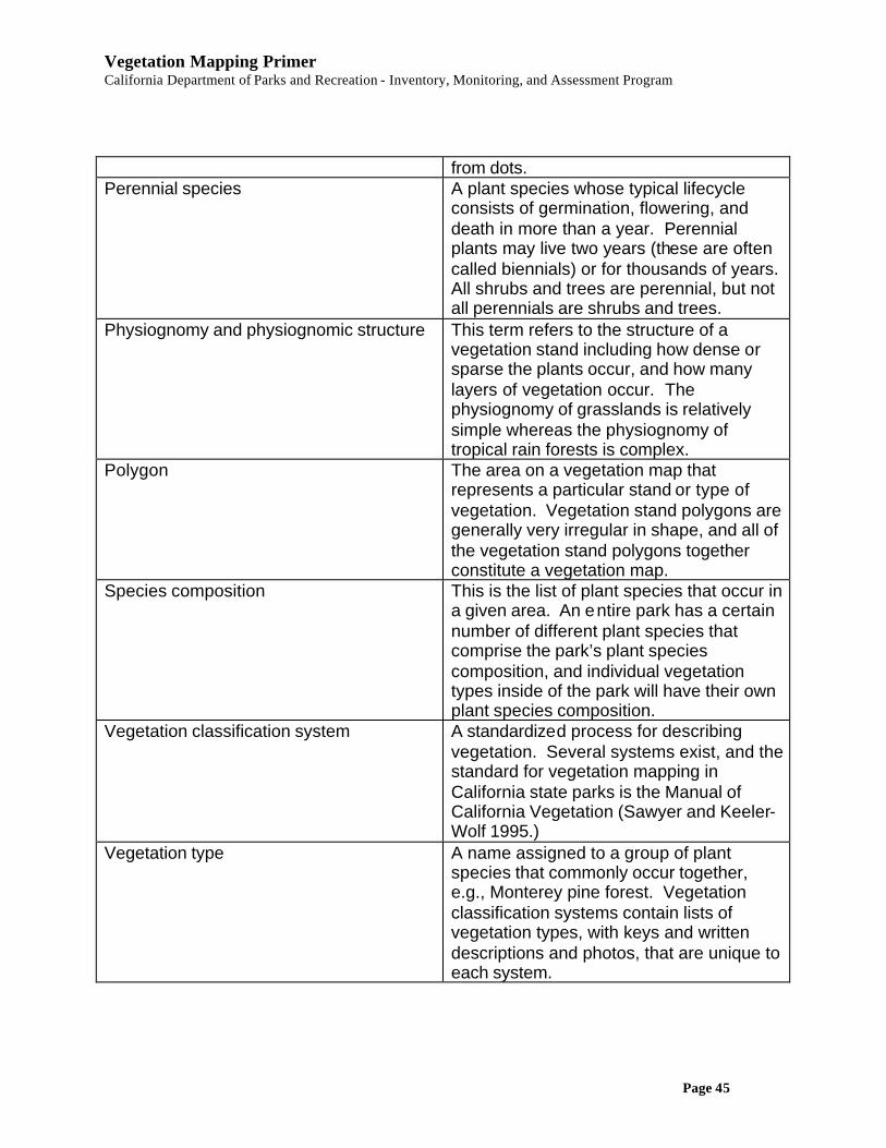
Vegetation Mapping Primer California Department of Parks and Recreation - Inventory, Monitoring, and Assessment Program
Page 45
from dots. Perennial species A plant species whose typical lifecycle
consists of germination, flowering, and death in more than a year. Perennial plants may live two years (these are often called biennials) or for thousands of years. All shrubs and trees are perennial, but not all perennials are shrubs and trees.
Physiognomy and physiognomic structure This term refers to the structure of a vegetation stand including how dense or sparse the plants occur, and how many layers of vegetation occur. The physiognomy of grasslands is relatively simple whereas the physiognomy of tropical rain forests is complex.
Polygon The area on a vegetation map that represents a particular stand or type of vegetation. Vegetation stand polygons are generally very irregular in shape, and all of the vegetation stand polygons together constitute a vegetation map.
Species composition This is the list of plant species that occur in a given area. An entire park has a certain number of different plant species that comprise the park’s plant species composition, and individual vegetation types inside of the park will have their own plant species composition.
Vegetation classification system A standardized process for describing vegetation. Several systems exist, and the standard for vegetation mapping in California state parks is the Manual of California Vegetation (Sawyer and Keeler-Wolf 1995.)
Vegetation type A name assigned to a group of plant species that commonly occur together, e.g., Monterey pine forest. Vegetation classification systems contain lists of vegetation types, with keys and written descriptions and photos, that are unique to each system.

Vegetation Mapping Primer California Department of Parks and Recreation - Inventory, Monitoring, and Assessment Program
Page 46
REFERENCES AND LINKS Cheatham, N.H. and J.R. Haller. An annotated list of California habitat types. University of California Natural Land and Water Reserves System, 1975. Ecological Society of America Panel on Vegetation Classification http://esa.sdsc.edu/vegwebpg.htm Federal Geographic Data Committee Vegetation subcommittee: http://biology.usgs.gov/fgdc.veg/ Jepson, W.L., R. Beidleman, and B. Ertter. 2000. Willis Linn Jepson’s “Mapping in forest botany”. Madrono 47(4)269-272. Lillesand, T.M. and R.W. Kiefer. 1994. Remote sensing and image interpretation. John Wiley & Sons, Inc., New York, ISBN 0-471-57783-9. 750 p. List of vegetation maps: http://www.lib.berkeley.edu/EART/vegmaps3.html#noamer Mayer, Kenneth E. and William F. Laudenslayer. 1988. A Guide to Wildlife Habitats of California. California Department of Fish and Game, Sacramento, California. 168 p. Natural Heritage Division, California Department of Fish and Game. 1998. Vegetation mapping of Anza-Borrego Desert State Park and environs: A report to the California Department of Parks and Recreation. Sacramento, CA. 165 p. National Park Service, 1994. http://biology.usgs.gov/npsveg/standards.html Sawyer, John O. and Todd Keeler-Wolf. 1995. A Manual of California Vegetation. California Native Plant Society, Sacramento, California. ISBN 0-943460-26-2. 471 p. Terrestrial Vegetation of the United States - The National Vegetation Classification System: Volumes I and II http://www.abi.org/publications/icec/

Vegetation Mapping Primer California Department of Parks and Recreation - Inventory, Monitoring, and Assessment Program
Page 47
Table 4-1. A hierarchal vegetation classification system. United States National Vegetation Classification (USNVC) - The Association for Biodiversity’s vegetation classification system. It is the basis for the Federal Geographic Data Committee National Vegetation Classification Standard and the Manual of California Vegetation. See table below for comparison. ABI USNVC FGDC NVCS Example
Physiognomic Levels
System Terrestrial
Division Vegetated
Order Tree
Class Class Woodland
Subclass Subclass Evergreen Woodland
Group Group Temperate or subpolar needle-leaved evergreen woodland
Subgroup Subgroup Natural or semi-natural vegetation
Formation Formation Rounded-crowned temperate or subpolar needle-leaved evergreen woodland
Floristic Levels
Alliance = series
Alliance (not finally adopted)
Juniperus scopularum Woodland
Association = plant community
Association (not finally adopted)
Juniperus scopularum/Oryzopsis micrantha Woodland

Vegetation Mapping Primer California Department of Parks and Recreation - Inventory, Monitoring, and Assessment Program
Page 48
Table 4-2. California Wildlife Habitat Relationships system habitat types.27
There are 59 terrestrial and aquatic wildlife habitat types in the CWHR system -- 27 tree types, 12 shrub types, 6 herbaceous types, 9 agricultural and developed habitats, 4 aquatic types, and 1 non-vegetated type. The original 53 habitat types are described in detail in the CWHR publication entitled:
A Guide to Wildlife Habitats of California. 1988. Edited by Kenneth E. Mayer and William F. Laudenslayer, Jr. State of California, Resources Agency, Department of Fish and Game, Sacramento, CA. 166 pp.
HABITAT TYPE
DOMINANT SPECIES or
DOMINANT ASSOCIATED SPECIES
1 Alkali Desert Scrub (ASC) Saltbush, Sagebrush, Creasotebush
2 Alpine Dwarf-Shrub (ADS) Creambush Oceanspray, Greene Goldenweed, Mountain White Heather
3 Annual Grassland (AGS) Wild Oats, Soft Chess, Brome
4 Aspen (ASP) Willows, Alders, Black Cottonwood
5 Barren (BAR) Rock, Pavement, Sand
6 Bitterbrush (BBS) Big Sagebrush, Rabbitbrush, Mormon Tea
7 Blue Oak Woodland (BOW) Live Oak, Valley Oak, Juniper
8 Blue Oak-Foothill Pine (BOP) Interior Live Oak, Valley Oak, California Buckeye
9 Chamise-Redshank Chaparral (CRC) Toyon, Ceanothus, Sugar Sumac
10 Closed Cone Pine-Cypress (CPC)
Tecate Cypress, Cuyamaca, Foothill Pine
11 Coastal Oak Woodland (COW) White Oak, California Black Oak, Engelmann Oak
12 Coastal Scrub (CSC) Lupine, Coyotebush, Sagebrush
13 Deciduous Orchard (DOR) Almonds, Walnuts, Peaches
14 Desert Riparian (DRI) Tamarisk, Velvet Ash, Mesquite
27 See http://www.dfg.ca.gov/whdab/html/habitats.html

Vegetation Mapping Primer California Department of Parks and Recreation - Inventory, Monitoring, and Assessment Program
Page 49
HABITAT TYPE
DOMINANT SPECIES or
DOMINANT ASSOCIATED SPECIES
15 Desert Scrub (DSC) Creasotebush, Catclaw Acacia, Desert Agave
16 Desert Succulent Shrub (DSS) Octillo, Mojave Yucca, Desert Agave
17 Desert Wash (DSW) Paloverde, Desert Ironwood, Mesquite
18 Douglas Fir (DFR) Live oak, Tanoak, Ponderosa Pine
19 Dryland Grain Crops (DGR) Cereal Rye, Barley, Wheat
20 Eastside Pine (EPN) Ponderosa Pine, Jeffrey Pine, White Fir
21 Estuarine (EST) Plankton, Algae, Eel Grass
22 Eucalyptus (EUC) Blue Gum, Red Gum
23 Evergreen Orchard (EOR) Oranges, Avocados, Lemons
24 Fresh Emergent Wetland (FEW) Big Leaf Sedge, Bulrush, Redroot NutGrass
25 Irrigated Grain Crops (IGR) Corn, Dry Beans, Safflower
26 Irrigated Hayfield (IRH) Alfalfa, Hay
27 Irrigated Row and Field Crops (IRF) Tomatoes, Cotton, Lettuce
28 Jeffrey Pine (JPN) Ponderosa Pine, Coulter Pine, Sugar Pine
29 Joshua Tree (JST) Juniper, Singleleaf Pinyon, Mojave Yucca
30 Juniper (JUN) White Fir, Jeffrey Pine, Ponderosa Pine
31 Klamath Mixed Conifer (KMC) White Fir, Douglas-Fir, Ponderosa Pine
32 Lacustrine (LAC) Plankton, Duckweed, Water Willies
33 Lodgepole Pine (LPN) Aspen, Mountain Hemlock, Red Fir
34 Low Sage (LSG) Rabbitbrush, Bitterbrush, Winter Fat
35 Marine (MAR) Plankton, Algae, Kelp
36 Mixed Chaparral (MCH) Oaks, Ceanothus, Manzanita
37 Montane Chaparral ((MCP) Ceanothus, Manzanita, Bitter Cherry
38 Montane Hardwood (MHW) Canyon Live Oak, Douglas Fir, Knobcone Pine
39 Montane Hardwood-Conifer (MHC)
Ponderosa Pine, Douglas Fir, Incense Cedar
40 Montane Riparian (MRI) Black Cottonwood, White Alder, Bigleaf
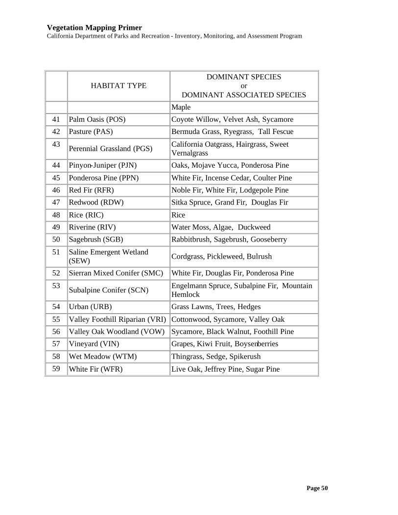
Vegetation Mapping Primer California Department of Parks and Recreation - Inventory, Monitoring, and Assessment Program
Page 50
HABITAT TYPE
DOMINANT SPECIES or
DOMINANT ASSOCIATED SPECIES
Maple
41 Palm Oasis (POS) Coyote Willow, Velvet Ash, Sycamore
42 Pasture (PAS) Bermuda Grass, Ryegrass, Tall Fescue
43 Perennial Grassland (PGS) California Oatgrass, Hairgrass, Sweet Vernalgrass
44 Pinyon-Juniper (PJN) Oaks, Mojave Yucca, Ponderosa Pine
45 Ponderosa Pine (PPN) White Fir, Incense Cedar, Coulter Pine
46 Red Fir (RFR) Noble Fir, White Fir, Lodgepole Pine
47 Redwood (RDW) Sitka Spruce, Grand Fir, Douglas Fir
48 Rice (RIC) Rice
49 Riverine (RIV) Water Moss, Algae, Duckweed
50 Sagebrush (SGB) Rabbitbrush, Sagebrush, Gooseberry
51 Saline Emergent Wetland (SEW) Cordgrass, Pickleweed, Bulrush
52 Sierran Mixed Conifer (SMC) White Fir, Douglas Fir, Ponderosa Pine
53 Subalpine Conifer (SCN) Engelmann Spruce, Subalpine Fir, Mountain Hemlock
54 Urban (URB) Grass Lawns, Trees, Hedges
55 Valley Foothill Riparian (VRI) Cottonwood, Sycamore, Valley Oak
56 Valley Oak Woodland (VOW) Sycamore, Black Walnut, Foothill Pine
57 Vineyard (VIN) Grapes, Kiwi Fruit, Boysenberries
58 Wet Meadow (WTM) Thingrass, Sedge, Spikerush
59 White Fir (WFR) Live Oak, Jeffrey Pine, Sugar Pine

Vegetation Mapping Primer California Department of Parks and Recreation - Inventory, Monitoring, and Assessment Program
Page 51
Table 5-1. Crosswalk of various vegetation classification systems. The following table is a crosswalk developed by the California Department of Fish and Game. The names of habitat types described in the California Wildlife Habitat Relationships System are crossed with other vegetation classification systems including Calveg (CAL), Holland (HOL), Manual of California Vegetation (MCV), UNESCO (UNE), and Cheatham and Haller (CHH).

Vegetation Mapping Primer California Department of Parks and Recreation - Inventory, Monitoring, and Assessment Program
Page 52
Table 6-1. Map scale comparison table.
Scale
Engineering Scale
U.S. National Map Accuracy
Standard (at given scale)
Note
1:1,200 1" = 100' +/- 3.33 feet Large Scale 1:2,400 1" = 200' +/- 6.67 feet 1:4,800 1" = 400' +/- 13.33 feet 1:9,600 1" = 800' +/- 26.67 feet 1:10,000 1” = 833’ +/- 27.78 feet 1:12,000 1" = 1000' +/- 33.33 feet 1:24,000 1" = 2000' +/- 40.00 feet 7.5 min quad 1:62,500 1” = 5,197’ +/- 100.00 feet 15 min quad 1:63,360 1" = 1.0 mile +/- 105.60 feet 1:100,000 1” = 1.6 mile +/- 166.67 feet Small Scale Longitude 1 degree at equator =
69.172 miles; 1 minute = 1.15± miles = 6076.113 feet or 1 nautical mile; 1 second = 101± feet; (1 knot/hr = 1 degree)
Longitude distance per degree decreases as you move north or south of the equator, 1º at 32º 30’ north (the Mexico/California border) = 58± miles, 1º at 42º north (Oregon/Calif border) = 51± miles.
Latitude 1 degree = 68.704 miles 1 minute = 1.15± miles 1 second = 101± feet
The difference in 1º latitude distance from the equator to the north/south pole is only 0.698 miles.
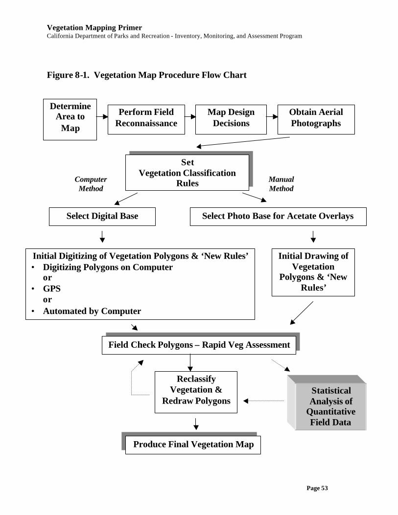
Vegetation Mapping Primer California Department of Parks and Recreation - Inventory, Monitoring, and Assessment Program
Page 53
Figure 8-1. Vegetation Map Procedure Flow Chart
Determine Area to
Map
Perform Field Reconnaissance
Obtain Aerial Photographs
Map Design Decisions
Set Vegetation Classification
Rules
Select Digital Base Select Photo Base for Acetate Overlays
Initial Drawing of Vegetation
Polygons & ‘New Rules’
Initial Digitizing of Vegetation Polygons & ‘New Rules’ • Digitizing Polygons on Computer
or • GPS
or • Automated by Computer
Field Check Polygons – Rapid Veg Assessment
Statistical Analysis of
Quantitative Field Data
Reclassify Vegetation &
Redraw Polygons
Produce Final Vegetation Map
Computer Method
Manual Method

Vegetation Mapping Primer California Department of Parks and Recreation - Inventory, Monitoring, and Assessment Program
Page 54
Attachment 8-1 CNPS Vegetation Rapid Assessment Protocol.