Vector AutoRegression Model/Eduardo Rossi -...
34
Universit` a di Pavia Vector AutoRegression Model Eduardo Rossi
-
Upload
duonghuong -
Category
Documents
-
view
224 -
download
0
Transcript of Vector AutoRegression Model/Eduardo Rossi -...

Universita di Pavia
Vector AutoRegression Model
Eduardo Rossi

VAR
Vector autoregressions (VARs) were introduced into empirical
economics by C.Sims (1980), who demonstrated that VARs provide a
flexible and tractable framework for analyzing economic time series.
Identification issue: since these models don’t dichotomize variables
into “endogenous” and “exogenous”, the exclusion restrictions used to
identify traditional simultaneous equations models make little sense.
A Vector Autoregression model (VAR) of order p is written as:
yt = c+Φ1yt−1 + . . .+Φpyt−p + ǫt
yt : (N × 1) Φi : (N ×N) ∀i, ǫt : (N × 1)
E(ǫt) = 0 E(ǫtǫ′τ ) =
Ω t = τ
0 t 6= τ
Ω positive definite matrix.
Eduardo Rossi c© - Time Series Econometrics 11 2

VAR(p)
A VAR is a vector generalization of a scalar autoregression.
The VAR is a system in which each variable is regressed on a
constant and p of its own lags as well as on p lags of each of the other
variables in the VAR.
[IN −Φ1L− · · · −ΦpLp]yt = c+ ǫt
Φ(L)yt = c+ ǫt
with
Φ(L) = [IN −Φ1L− · · · −ΦpLp]
Φ(L) (N ×N) matrix polynomial in L.
Eduardo Rossi c© - Time Series Econometrics 11 3

VAR(p) - Stationarity
The element (i, j) in Φ(L) is a scalar polynomial in L
δij − φ(1)ij L− φ
(2)ij L2 − . . . φ
(p)ij Lp
δij =
1 i = j
0 i 6= j
Stationarity: A vector process is said covariance stationary if its
first and second moments, E[yt] and E[yty′t−j ] respectively, are
independent of the date t.
Eduardo Rossi c© - Time Series Econometrics 11 4

VAR(1)
yt = c+Φ1yt−1 + ǫt
First equation:
y1t = c1 + φ(1)11 y1t−1 + φ
(1)12 y2t−1 + . . .+ φ
(1)1NyNt−1 + ǫ1t
yt = c+Φ1 [c+Φ1yt−2 + ǫt−1] + ǫt
= c+Φ1c+Φ21yt−2 + ǫt +Φ1ǫt−1
yt = . . .
yt = c+Φ1c+ . . .+Φk−11 c+Φk
1yt−k + ǫt +Φ1ǫt−1 + . . .+Φk−11 ǫt−k+1
E[yt] =k−1∑
j=0
Φj1c+Φk
1E[yt−k]
The value of this sum depends on the behavior of Φj1 as j increases.
Eduardo Rossi c© - Time Series Econometrics 11 5

Stability of VAR(1)
Let λ1, λ2, . . . , λN be the eigenvalues of Φ1, the solutions to the
characteristic equation
|Φ1 − λIN | = 0
then, if the eigenvalues are all distinct
Φ1 = QMQ−1
Φk1 = QMkQ−1
Mk = diag(λk1 , λ
k2 , . . . , λ
kN )
If |λi| < 1, i = 1, . . . , N
Φk → 0, k → ∞
If |λi| ≥ 1, ∀i then one or more elements of Mk are not vanishing,
and may be tending to ∞.
Eduardo Rossi c© - Time Series Econometrics 11 6

VAR(P) Companion form
VAR(p):
yt = Φ1yt−1 + . . .+Φpyt−p + ǫt
as a VAR(1) (Companion Form):
ξt = Fξt−1 + vt
ξt =
yt
...
yt−p+1
(Np× 1) ξt−1 =
yt−1
...
yt−p
(Np× 1)
Eduardo Rossi c© - Time Series Econometrics 11 7

VAR(P) Companion form
F =
Φ1 Φ2 . . . Φp−1 Φp
IN 0 . . . 0 0
0 IN . . . 0 0...
......
...
0 0 . . . IN 0
(Np×Np) vt =
ǫt
0...
0
(Np×1)
E[vtv′τ ] =
Q t = τ
0 t 6= τQ =
Ω 0 . . . 0
0 0 . . . 0
......
...
0 0 . . . 0
(Np×Np)
Eduardo Rossi c© - Time Series Econometrics 11 8
Stability of VAR(p)
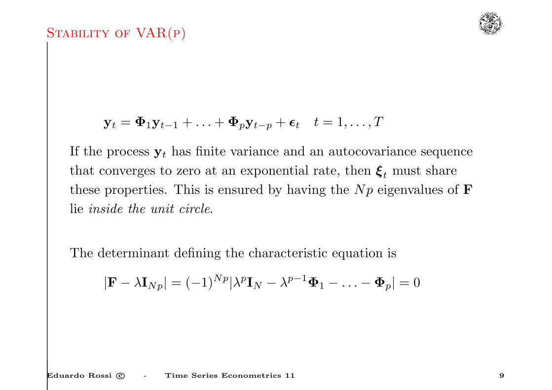
yt = Φ1yt−1 + . . .+Φpyt−p + ǫt t = 1, . . . , T
If the process yt has finite variance and an autocovariance sequence
that converges to zero at an exponential rate, then ξt must share
these properties. This is ensured by having the Np eigenvalues of F
lie inside the unit circle.
The determinant defining the characteristic equation is
|F− λINp| = (−1)Np|λpIN − λp−1Φ1 − . . .−Φp| = 0
Eduardo Rossi c© - Time Series Econometrics 11 9

Stability of VAR(p)
The required condition is that the roots of the equation
|λpIN − λp−1Φ1 − . . .−Φp| = 0
a polynomial of order Np must lie inside the unit circle.
Stability condition can also be expressed as the roots of
|Φ(z)| = 0
lie outside the unit circle, where Φ(z) is a (N ×N) matrix
polynomial in the lag operator of order p.
Eduardo Rossi c© - Time Series Econometrics 11 10

Stability of VAR(p)
When p = 1, the roots of
|IN −Φ1z| = 0
outside the unit circle, i.e. |z| > 1, implies that the eigenvalues of Φ1
be inside the unit circle. Note that the eigenvalues, roots of
|Φ1 − λIN | = 0, are the reciprocal of the roots of |IN −Φ1z| = 0.
Eduardo Rossi c© - Time Series Econometrics 11 11

Stability of VAR(p)
Three conditions are necessary for stationarity of the VAR(p) model:
• Absence of mean shifts;
• The vectors ǫt are identically distributed, ∀t;
• Stability condition on F.
If the process is covariance stationary we can take the expectations of
both sides of
yt = c+Φ1yt−1 + . . .+Φpyt−p + ǫt
µ = c+Φ1µ+ . . .+Φpµ
µ = [IN −Φ1 . . .−Φp]−1c
= Φ(1)−1c
Eduardo Rossi c© - Time Series Econometrics 11 12
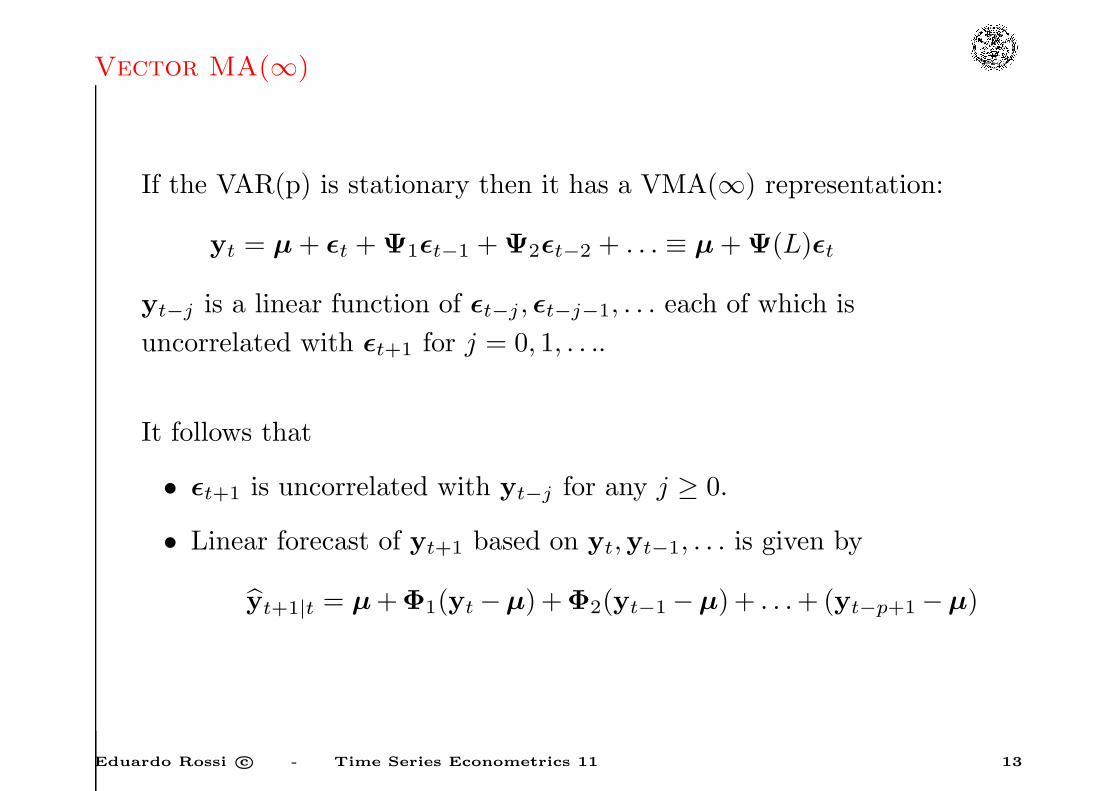
Vector MA(∞)
If the VAR(p) is stationary then it has a VMA(∞) representation:
yt = µ+ ǫt +Ψ1ǫt−1 +Ψ2ǫt−2 + . . . ≡ µ+Ψ(L)ǫt
yt−j is a linear function of ǫt−j , ǫt−j−1, . . . each of which is
uncorrelated with ǫt+1 for j = 0, 1, . . ..
It follows that
• ǫt+1 is uncorrelated with yt−j for any j ≥ 0.
• Linear forecast of yt+1 based on yt,yt−1, . . . is given by
yt+1|t = µ+Φ1(yt −µ) +Φ2(yt−1 −µ) + . . .+ (yt−p+1 −µ)
Eduardo Rossi c© - Time Series Econometrics 11 13

Forecasting with VAR
ǫt+1 can be interpreted as the fundamental innovation in yt+1, that
is the error in forecasting yt+1 on the basis of a linear function of a
constant and yt,yt−1, . . ..
A forecast of yt+s on the basis of yt,yt−1, . . . will take the form
yt+s|t = µ+F(s)11 (yt−µ)+F
(s)12 (yt−1−µ)+ . . .+F
(s)1p (yt−p+1−µ)
The moving average matrices Ψj can be calculated as:
Ψ(L) = [Φ(L)]−1
Ψ(L)Φ(L) = IN
Eduardo Rossi c© - Time Series Econometrics 11 14

VMA coefficient matrices
[IN +Ψ1L+Ψ2L2 + . . .][IN −Φ1L−Φ2L
2 + . . .−ΦpLp] = IN
Setting the coefficient on L1 equal to the zero matrix,
Ψ1 −Φ1 = 0
on L2
Ψ2 = Ψ1Φ1 +Φ2
In general for Ls
Ψs = Φ1Ψs−1 + . . .+ΦpΨs−p s = 1, 2, . . .
Ψ0 = IN , Ψs = 0 s < 0
Eduardo Rossi c© - Time Series Econometrics 11 15

VMA coefficient matrices
The innovation in the MA(∞) representation is ǫt, the fundamental
innovation for y.
There are alternative MA representation based on VWN processes
other than ǫt.
Let H be a nonsingular (N ×N) matrix
ut ≡ Hǫt
ut ∼ VWN .
yt = µ+H−1Hǫt +Ψ1H−1Hǫt−1 + . . .
= µ+ J0ut + J1ut−1 + J2ut−2 + . . .
Js ≡ ΨsH−1
Eduardo Rossi c© - Time Series Econometrics 11 16

VMA coefficient matrices
For example H can be any matrix that diagonalizes Ω, the var-cov of
ǫt,
HΩH′ = D
the elements of ut are uncorrelated with one another.
It is always possible to write a stationary VAR(p) process as a
convergent infinite MA of a VWN whose elements are mutually
uncorrelated.
To obtain the MA representation for the fundamental innovations, we
must impose Ψ0 = IN (while J0 is not the identity matrix).
Eduardo Rossi c© - Time Series Econometrics 11 17

Assumptions implicit in a VAR
• For a covariance stationary process, the parameters c,Φ1, . . . ,Φp
could be defined as the coefficients of the projections of yt on
1,yt−1,yt−2, . . . ,yt−p.
• ǫt is uncorrelated with yt−1, . . . ,yt−p by the definition of
Φ1, . . . ,Φp.
• The parameters of a VAR can be estimated consistently with n
OLS regressions.
• ǫt defined by this projection is uncorrelated with
yt−p−1,yt−p−2, . . .
• The assumption of yt ∼ V AR(p) is basically the assumption that
p lags are sufficient to summarize the dynamic correlations
between elements of y.
Eduardo Rossi c© - Time Series Econometrics 11 18
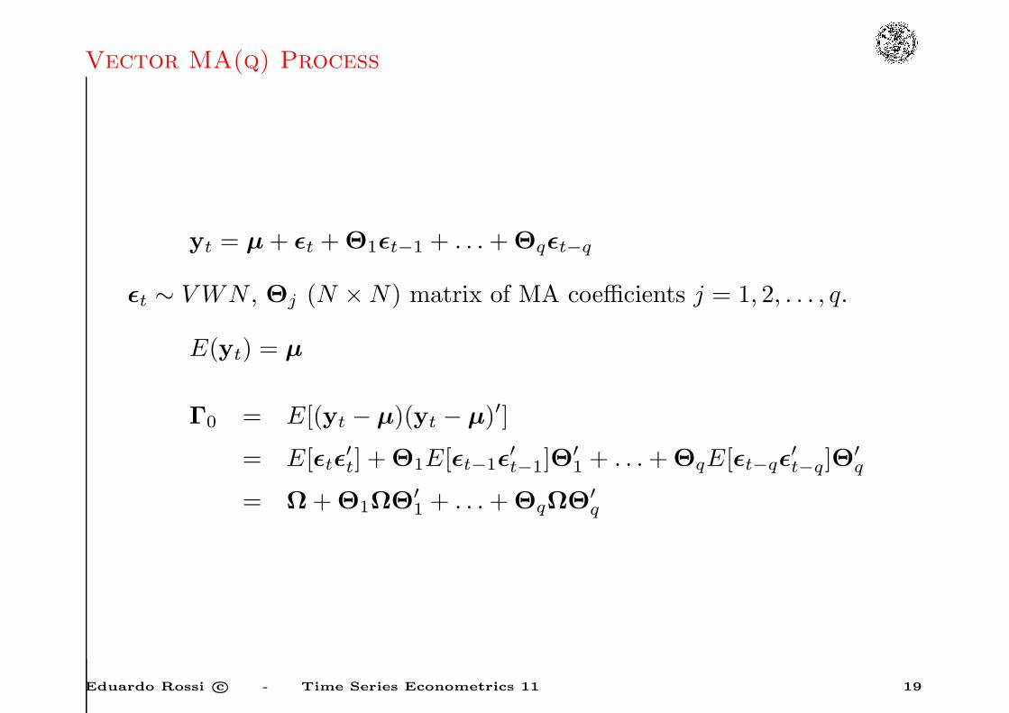
Vector MA(q) Process
yt = µ+ ǫt +Θ1ǫt−1 + . . .+Θqǫt−q
ǫt ∼ VWN , Θj (N ×N) matrix of MA coefficients j = 1, 2, . . . , q.
E(yt) = µ
Γ0 = E[(yt − µ)(yt − µ)′]
= E[ǫtǫ′t] +Θ1E[ǫt−1ǫ
′t−1]Θ
′1 + . . .+ΘqE[ǫt−qǫ
′t−q]Θ
′q
= Ω+Θ1ΩΘ′1 + . . .+ΘqΩΘ′
q
Eduardo Rossi c© - Time Series Econometrics 11 19

Vector MA(q) Process
Γj = E[(ǫt +Θ1ǫt−1 + . . .+Θqǫt−q)(ǫt−j +Θ1ǫt−j−1 + . . .+Θqǫt−j−q)′]
Γj =
ΘjΩ+Θj+1ΩΘ′1 +Θj+2ΩΘ′
2 + . . .+ΘqΩΘ′q−1 j = 1, . . . , q
ΩΘ′−j +Θ1ΩΘ′
−j+1 + . . .+Θq+jΩΘ′q j = −1, . . . ,−q
0 |j| > q
Θ0 = IN . Any VMA(∞) is covariance stationary.
Eduardo Rossi c© - Time Series Econometrics 11 20
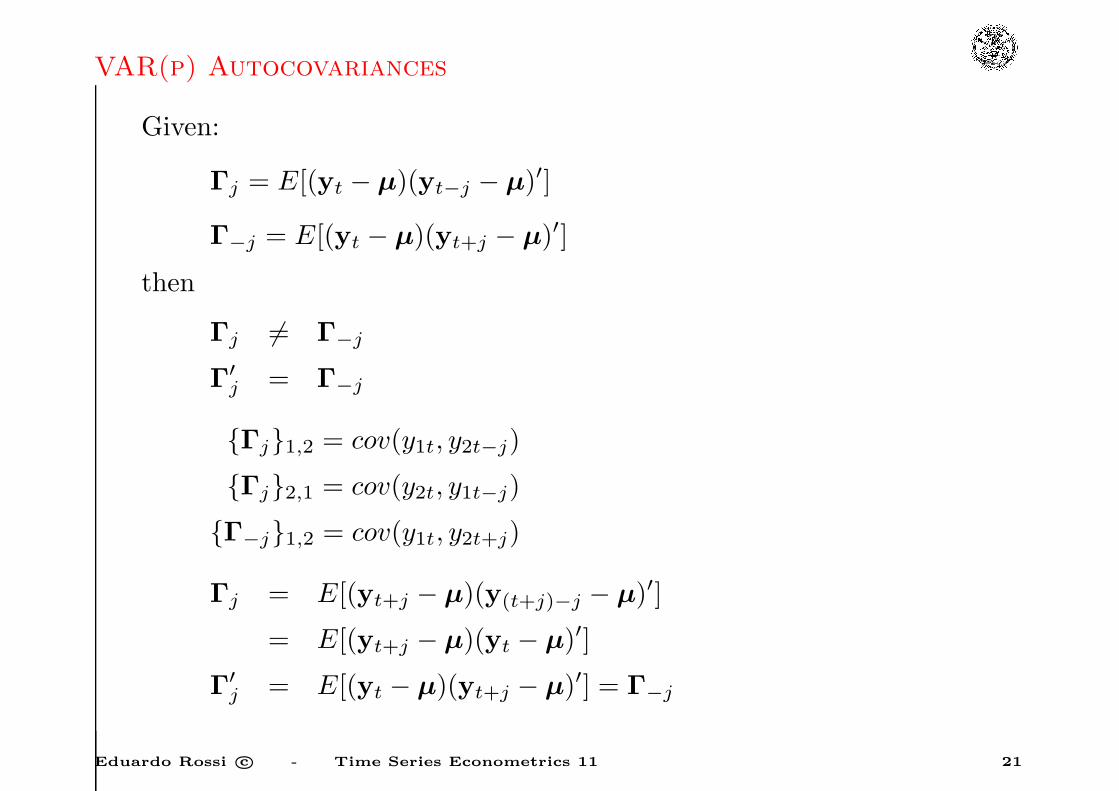
VAR(p) Autocovariances
Given:
Γj = E[(yt − µ)(yt−j − µ)′]
Γ−j = E[(yt − µ)(yt+j − µ)′]
then
Γj 6= Γ−j
Γ′j = Γ−j
Γj1,2 = cov(y1t, y2t−j)
Γj2,1 = cov(y2t, y1t−j)
Γ−j1,2 = cov(y1t, y2t+j)
Γj = E[(yt+j − µ)(y(t+j)−j − µ)′]
= E[(yt+j − µ)(yt − µ)′]
Γ′j = E[(yt − µ)(yt+j − µ)′] = Γ−j
Eduardo Rossi c© - Time Series Econometrics 11 21

VAR(p) Autocovariances
Companion form:
ξt = Fξt−1 + vt
Σ = E[ξtξ′t]
Σ = E
yt − µ
yt−1 − µ
...
yt−p+1 − µ
[(yt − µ)′ . . . (yt−p+1 − µ)′]
=
Γ0 Γ1 . . . Γp−1
Γ′1 Γ0 . . . Γp−2
......
Γ′p−1 Γ′
p−2 . . . Γ0
(Np×Np)
Eduardo Rossi c© - Time Series Econometrics 11 22

VAR(p) Autocovariances
E[ξtξ′t] = E[(Fξt−1 + vt)(Fξt−1 + vt)
′]
= FE(ξt−1ξ′t−1)F
′ + E(vtv′t)
where FE(ξt−1v′t) = 0.
Σ = FΣF′ +Q
vec(Σ) = vec(FΣF′) + vec(Q)
vec(Σ) = vec(FΣF′) + vec(Q)
vec(Σ) = (F⊗ F)vec(Σ) + vec(Q)
= [I(Np)2 − (F⊗ F)]−1vec(Q)
The eigenvalues of (F⊗ F) are all of the form λjλj where λi and λj
are eigenvalues of F. Since |λi| < 1, ∀i, it follows that all eigenvaluesof (F⊗ F) are inside the unit circle |I(Np)2 − (F⊗ F)| 6= 0.
Eduardo Rossi c© - Time Series Econometrics 11 23

VAR(p) Autocovariances
The j -th autocovariance of ξt is
E[ξtξ′t−j ] = FE[ξt−1ξ
′t−j ] + E[vtξ
′t−j ]
Σj = FΣj−1
Σj = FjΣ j = 1, 2, . . .
The j -th autocovariance of yt is given by the first rows and n
columns of Σj
Γj = Φ1Γj−1 + . . .+ΦpΓj−p
Eduardo Rossi c© - Time Series Econometrics 11 24

Maximum Likelihood Estimation
yt = c+Φ1yt−1 + . . .+Φpyt−p + ǫt (1)
ǫt ∼ i.i.d.N(0,Ω)
(T + p) observations. Conditioning on the first p observations we
estimate using the last T observations.
Conditional likelihood:
fYT ,YT−1,...,Y1|Y0,...,Y1−p(yT , . . . ,y1|y0, . . . ,y1−p; θ)
Eduardo Rossi c© - Time Series Econometrics 11 25

Maximum Likelihood Estimation
θ = (c′, vec(Φ1)′, vec(Φ2)
′, . . . , vec(Φp)′, vech(Ω)′)′
yt|yt−1, . . . ,y−p+1 ∼ N(c+Φ1yt−1 + . . .+Φpyt−p,Ω)
xt =
1
yt−1
...
yt−p
(Np+ 1)× 1
Π′ ≡[c Φ1 Φ2 . . . Φp
](N × (Np+ 1))
E(yt|yt−1, . . . ,y−p+1) = Π′xt
Eduardo Rossi c© - Time Series Econometrics 11 26

Maximum Likelihood Estimation
fYt|Yt−1,...,Y1−p(yt|yt−1, . . . ,y1−p; θ) =
(2π)−n2 |Ω−1| 12 exp
(−1
2(yt −Π′xt)
′Ω−1(yt −Π′xt)
)
The joint density, conditional on the y0, . . . ,y1−p
fYt,...,Y1|Y0,...,Y1−p(yt, . . . ,y1|y0, . . . ,y1−p; θ) = fYt|Yt−1,...,Y1−p
(θ)×fYt−1,...,Y1|Y0,...,Y1−p
(θ)
Eduardo Rossi c© - Time Series Econometrics 11 27

Maximum Likelihood Estimation
Recursively, the likelihood function for the full sample, conditioning
on y0, . . . ,y1−p, is the product of the single conditional densities:
fYT ,...,Y1|Y0,...,Y1−p=
T∏
t=1
fYt|Yt−1,...,Y1−p(yt|yt−1, . . . ,y1−p; θ)
The log likelihood function:
L(θ) = −TN
2log (2π)+
T
2log |Ω−1|−1
2
T∑
t=1
[(yt −Π′xt)
′Ω−1(yt −Π′xt)]
Eduardo Rossi c© - Time Series Econometrics 11 28

Maximum Likelihood Estimation
The ML estimate of Π:
Π′ =
[T∑
t=1
ytx′t
][T∑
t
xtx′t=1
]−1
The j -th row of Π′ is:
u′jΠ
′ = u′j
[T∑
t=1
ytx′t
][T∑
t
xtx′t
]−1
This is the estimated coefficient vector from an OLS regression of yjton xt. ML estimates are found by an OLS regression of yjt on a
constant and p lags of all the variables in the system.
The ML estimate of Ω is given by:
Ω =1
T
T∑
t=1
ǫtǫ′t
Eduardo Rossi c© - Time Series Econometrics 11 29

Maximum Likelihood Estimation
Asymptotic distribution of Π
The ML estimates Π and Ω will give consistent estimates of the
population parameters even if the true innovations are non-gaussian:
Φ(L)yt = ǫt
ǫt ∼ i.i.d.(0,Ω)
E[ǫitǫjtǫltǫmt] < ∞ ∀i, j, l,m
the roots of
|IN −Φ1z − . . .−Φpzp| = 0
Let K ≡ N · p+ 1, x′t (1×K):
x′t = [1 ,y′
t ,y′t−1 , . . . ,y
′t−p]
πT = vec(ΠT )
Eduardo Rossi c© - Time Series Econometrics 11 30

Maximum Likelihood Estimation
πT =
π1,T
...
πN,T
πi,t =
(∑
t
xtx′t
)−1(∑
t
xtyit
)
ΩT =1
T
∑
t
ǫtǫ′t
ǫit = yit − x′tπi,T
Eduardo Rossi c© - Time Series Econometrics 11 31

Maximum Likelihood Estimation
Then,
1
T
∑
t
xtx′t
p→ Q = E (xtx′t)
πTp→ π
ΩTp→ Ω
√T (πT − π)
d→ N(0, (Ω⊗Q−1))√T (πi,T − π)
d→ N(0, (σ2iQ
−1))
σ2i = E(ǫ2it)
σ2i =
1
T
∑
t
ǫ2itp→ σ2
i
Eduardo Rossi c© - Time Series Econometrics 11 32
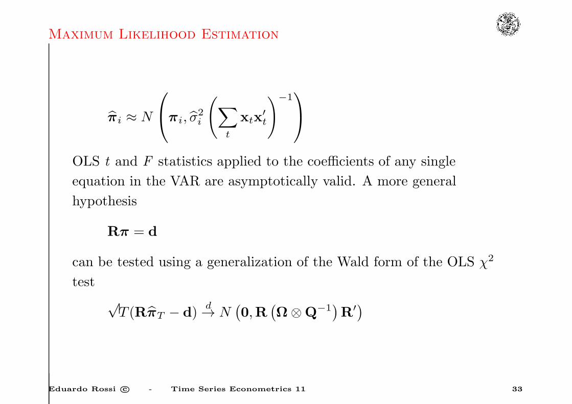
Maximum Likelihood Estimation
πi ≈ N
πi, σ
2i
(∑
t
xtx′t
)−1
OLS t and F statistics applied to the coefficients of any single
equation in the VAR are asymptotically valid. A more general
hypothesis
Rπ = d
can be tested using a generalization of the Wald form of the OLS χ2
test
√T (RπT − d)
d→ N(0,R
(Ω⊗Q−1
)R′)
Eduardo Rossi c© - Time Series Econometrics 11 33

Maximum Likelihood Estimation
ξ2(m) = T (RπT − d)′[R(ΩT ⊗ Q−1
T
)R′]−1
(RπT − d)
= (RπT − d)′[R(ΩT ⊗ (T QT )
−1)R′]−1
(RπT − d)
= (RπT − d)′
R
ΩT ⊗
(∑
t
xtx′t
)−1R′
−1
(RπT − d)
Eduardo Rossi c© - Time Series Econometrics 11 34