JOURNAL OF GEOMETRIC MECHANICS doi:10.3934/jgm.2012.4.xxc©American Institute of Mathematical SciencesVolume 4, Number 2, June 2012 pp. X–XX

VARIATIONAL INTEGRATORS FOR HAMILTONIZABLE

NONHOLONOMIC SYSTEMS

Oscar E. Fernandez

Department of MathematicsWellesley College

Wellesley, MA 02482, USA

Anthony M. Bloch

Department of Mathematics

University of MichiganAnn Arbor, MI 48109, USA

Peter J. Olver

School of MathematicsUniversity of Minnesota

Minneapolis, MN 55455, USA

Abstract. We report on new applications of the Poincare and Sundman time-transformations to the simulation of nonholonomic systems. These transfor-

mations are here applied to nonholonomic mechanical systems known to be

Hamiltonizable (briefly, nonholonomic systems whose constrained mechanicsare Hamiltonian after a suitable time reparameterization). We show how

such an application permits the usage of variational integrators for these non-

variational mechanical systems. Examples are given and numerical results arecompared to the standard nonholonomic integrator results.

Introduction. It is well known that the dynamical equations of motion of uncon-strained mechanical systems follow from a variational principle, namely Hamilton’sprinciple of stationary action [1, 26]. In the 1970s and 1980s several researchersdiscretized this continuous variational principle and developed the discrete Euler-Lagrange equations (see [27] and references therein for a historical account). Likeits continuous counterpart, this discrete variational mechanics preserves many ofthe constants of motion between timestep increments, such as the energy and mo-mentum, as well as the symplectic form, under appropriate assumptions [21, 27].The resulting numerical integrators, termed mechanical integrators, have found ap-plication in molecular dynamics simulations [34, 24, 23] and planetary motion [23],as well as in satellite dynamics [23]. For fixed timesteps, it was shown in [18] thata mechanical integrator for a non-integrable mechanical system with symmetry canat best preserve two of the three quantities mentioned above. For this reason, fixedtimestep mechanical integrators are named according to what invariants they dopreserve. In particular, mechanical integrators preserving the discretized symplec-tic form and momentum are known as variational integrators.

2000 Mathematics Subject Classification. Primary: 37J60; Secondary: 34K28.Key words and phrases. Nonholonomic Systems, Hamiltonization, Variational Integrators.

1

2 OSCAR E. FERNANDEZ, ANTHONY M. BLOCH AND PETER J. OLVER

Variational integrators for mechanical systems with position constraints (knownas holonomic constraints) were developed shortly after the formulation of discretevariational mechanics (see [32] and Section 3.4 of [27] and references therein). How-ever, for mechanical systems subject to non-integrable constraints on the velocities(known as nonholonomic systems), developing corresponding integrators remaineda challenge for some time. The inherent difficulty arises from the fact that theequations of motion of a general nonholonomic system on a symplectic manifold(T ∗Q,ω) (here ω is the symplectic form) follow not from Hamilton’s principle, butinstead from the Lagrange-d’Alembert principle [1]. The most immediate conse-quence is that the nonholonomic flow does not preserve the symplectic form ([8],Section 3.4.1). Thus, the basis of discrete variational mechanics (the discretizationof Hamilton’s principle) does not apply to nonholonomic systems. Despite this diffi-culty, the development of a “nonholonomic integrator” was achieved more recentlyin [9]. The authors discretized the Lagrange-d’Alembert principle to arrive at amechanical integrator which preserves the evolution of the discretized symplecticform ω under the nonholonomic flow. In addition, for a nonholonomic system withsymmetry, their nonholonomic integrator satisfies a discrete version of the nonholo-nomic momentum equation1.

Historically, although the fact that nonholonomic mechanics is not variational(meaning the governing equations of motion do not follow from Hamilton’s prin-ciple) was proved as early as 1899 by Korteweg [22], there have since been manyattempts to “Hamiltonize” nonholonomic systems. In light of Korteweg’s result, thisis impossible to accomplish for the “full” nonholonomic system, which is generally acoupled set of first-order kinematic equations (in the simplest case of linear homoge-neous nonholonomic constraints) and second-order dynamical equations. However,under certain symmetry conditions the kinematic equations decouple from the dy-namics, in which case one can investigate the possibility of “Hamiltonizing” thesecond-order dynamical equations. The most successful early attempts to do sowere made by the Russian mathematician S.A. Chaplygin in 1903, motivating thename Chaplygin System [1] (Section 5.4). In [6, 7] he showed that for nonholo-nomic systems in two degrees of freedom (q1, q2) which preserve a scaled symplecticform f(q1, q2)ω for some multiplier f ∈ C2(Q) one can define the time reparame-terization dτ = f(q) dt such that the nonholonomic equations become the Euler-Lagrange equations of the time-reparameterized nonholonomic Lagrangian. Thisresult is known as the Chaplygin Reducing Multiplier Theorem, and has been thesubject of recent renewed interest (see [15] and references therein). It has recentlybeen applied to nonholonomic Hamilton-Jacobi theory [31], and to the study of theintegrability of rolling bodies (see [4] and references therein).

In this paper we apply Chaplygin’s theorem to develop two new mechanicalintegrators for Chaplygin nonholonomic systems for which Chaplygin’s theoremapplies (termed Chaplygin Hamiltonizable). The mechanical integrators developed,in contrast to the nonholonomic integrator discussed above, are variational, that is,they are developed by discretizing Hamilton’s principle. The examples developedin Section 5 suggest that, in general, the new algorithms accurately simulate thesecond-order dynamics of the Chaplygin Hamiltonizable system, and in some casesoutperform the results obtained by the nonholonomic integrator. These results

1Unlike unconstrained mechanics, infinitesimal symmetries of nonholonomic systems do notnecessarily lead to momentum conservation laws. Instead, the corresponding momentum maps

evolve according to the nonholonomic momentum equation [1] (Section 5.5).

VARIATIONAL INTEGRATORS FOR HAMILTONIZABLE NONHOLONOMIC SYSTEMS 3

confirm earlier studies [29] showing that the combination of Hamiltonization andvariational integrators can lead to superior numerical schemes for simulating thedynamics of many of the relevant nonholonomic systems.

The paper is organized as follows. We begin with a review of nonholonomicmechanics in Section 1, followed by a review of variational and nonholonomic inte-grators in Section 2. We discuss Chaplygin’s theorem in more detail in Section 3in preparation for the introduction of the new integrators in Section 4. In Section4.1 we introduce the Hamiltonized discrete Euler-Lagrange algorithm, an integra-tor which proceeds in discretized τ -time. In Section 4.2 we introduce the Poincaretransformed Hamiltonized discrete Euler-Lagrange algorithm, which proceeds in t-time, and makes use of the so-called Poincare transformation [23] (Chapter 9).Finally, we compare the performance of the two new integrators with that of thenonholonomic integrator for three examples in Section 5, and indicate possible ap-plications and directions for future research in the Conclusion.

1. Nonholonomic Chaplygin systems. Consider a mechanical system on an n-dimensional Riemannian configuration manifold Q with metric g and with regularLagrangian L : TQ → R. We assume that L = T − V , where T : TQ → R isthe kinetic energy given by T (q, q) = 1

2gij qiqj , i, j = 1, . . . , n, where gij are the

components of g, and V : Q → R is the potential energy (we identify V with itslift to TQ). We note that we will adhere to the Einstein summation convention forrepeated indices throughout.

Suppose that we now define a constraint distribution D ⊂ TQ by the one-formsωaka=1, k < n, as

D = v ∈ TQ |ωa(v) = 0, a = 1, . . . , k. (1)

We will assume that the constraints are linear and homogeneous, so that locallyωa(v) = caj (q)qj , and that D has constant rank. Then the triple (Q,L,D) is knownas a nonholonomic mechanical system [1].

Now, suppose that a k-dimensional Lie group G acts on Q such that M := Q/Gis a manifold; this happens, for example, if G acts freely and properly on Q. Let gbe the Lie algebra of G, and ξQ the infinitesimal generator on Q corresponding toξ ∈ g. We assume that its lifted action leaves L and D invariant, and that at eachq ∈ Q, the tangent space TqQ can be decomposed as

TqQ = gQ ⊕Dq, where gQ|q = ξQ(q) | ξ ∈ g (2)

is the tangent to the orbit through q ∈ Q [1] (Section 2.8). Then we will call(Q,L,D, G) a Chaplygin nonholonomic system [1]. This setup gives rise to a princi-pal bundle π : Q→M , with principal connection A : TQ→ g such that kerA = D.This connection can then be used to decompose any tangent vector vq ∈ TqQ intohorizontal and vertical parts:

vq = hor(vq) + ver(vq), (3)

where hor(vq) = vq − (Aq(vq))Q(q), ver(vq) = (Aq(vq))Q(q).

We can now form the reduced velocity phase space TQ/G, and the LagrangianL induces the reduced Lagrangian l : TQ/G → R satisfying L = l πTQ, whereπTQ : TQ→ TQ/G is the standard projection. Furthermore, the decomposition (3)gives rise to the reduced constrained Lagrangian lc : TM → R given by lc(r, r) :=

4 OSCAR E. FERNANDEZ, ANTHONY M. BLOCH AND PETER J. OLVER

L(q,hor(q)), where r = π(q) and r = Tqπ(q). Locally, we will write the reducedconstrained Lagrangian as

lc(r, r) =1

2Gαβ(r)rαrβ − V (r), (4)

where henceforth Greek indices will range from 1 to m :=dim M = n−k, the indicesa, b, c will range from 1 to k = dim G, and where V : M → R is defined by V = V π.Since we will be dealing exclusively with the reduced constrained Lagrangian, wewill drop the overbar on V henceforth. The Gαβ are the components of the metric onthe reduced space M induced by g according to Gr(vr, wr) := gq(hor(vq),hor(wq)),where r = π(q).

To arrive at the local equations of motion of a Chaplygin nonholonomic systemwe pick a local trivialization, where Q = Q/G×G and the action of G is given byleft translation on the second factor, and choose coordinates r for the first factorand a basis ea of the Lie algebra g of G. The equations of motion then consist of asystem of second-order ordinary differential equations on M , together with a systemof first-order constraint equations [1]:

d

dt

∂lc∂rα− ∂lc∂rα

= −(∂l

∂ξa

)∗Baαβ rβ , (5)

ξa = −Aaα(r)rα. (6)

Here the star indicates that we have substituted the constraints (6) into (5) afterdifferentiation, and

Baαβ =∂Aaβ∂rα

− ∂Aaα∂rβ

− CabcAbαAcβ (7)

are the components of the curvature of A, where Cabc are the structure constants ofthe Lie algebra defined by [ea, eb] = Cabc.

As discussed in the Introduction, the full equations of motion, (5)-(6), cannotin general be derived from Hamilton’s principle [1, 17, 22]. In other words, non-holonomic mechanics is not variational, or said yet another way, (5)-(6) are notthe Euler-Lagrange equations for any Lagrangian, or of the canonical Hamiltonianequations for any Hamiltonian (unless of course Baαβ = 0, in which case the system

in actually holonomic)2.

2. Geometric integrators. As discussed in the Introduction, the discretizationof Hamilton’s principle produces a variational integrator while discretizing theLagrange-d’Alembert principle produces a nonholonomic integrator. Let us brieflyreview these discretizations.

2.1. Variational integrators. Suppose that one is interested in simulating thedynamics of a Hamiltonian system between the two times t = a and t = b. Beginby specifying the time steps a = t0 < t1 < . . . < tN = b with fixed step sizeh := ti+1− ti, i = 0, . . . , N−1, and define the discrete trajectory to be the sequence

qj0, . . . , qjN ∈ Q, j = 1, . . . , n, where qji ≈ qj(ti). Then, define the smooth map

2We should mention, however, that the full system (5)-(6) can in some cases be embedded, ina non-trivial way, in a larger system which is variational [14, 2].

VARIATIONAL INTEGRATORS FOR HAMILTONIZABLE NONHOLONOMIC SYSTEMS 5

Ld : Q×Q→ R which will approximate the action over each time step3:

Ld(qi, qi+1) ≈∫ ti+1

ti

L(q(t), q(t)) dt. (8)

One can then define the discrete action sum Sd(q0, . . . , qN ) by:

Sd(q0, . . . , qN ) =

N−1∑i=0

Ld(qi, qi+1) ≈∫ b

a

L(q(t), q(t)) dt. (9)

Then, taking variations of the discrete path (with fixed endpoints) leads to thediscrete Euler-Lagrange (DEL) equations [27]:

D1Ld(qi, qi+1) +D2Ld(qi−1, qi) = 0, i = 1, . . . , N − 1, (10)

where D1, D2 denote differentiation with respect to the first and second arguments,respectively, and where q = (q1, . . . , qn) on Q. The DEL equations (10), underappropriate regularity assumptions (see Section 7.2 in [8]), define the discrete timeevolution of the system via the map Φv : Q × Q → Q × Q given by Φv(qi−1, qi) =(qi, qi+1) (where the superscript reminds us that this is a variational integratoralgorithm). The explicit formula for Φv is only available when the DEL algorithm(10) is “explicit,” in the sense that one can explicitly solve for qi+1 = F (qi−1, qi)).This happens, for example, when the Lagrangian L has a constant kinetic energymetric g [27]. Otherwise, the algorithm (10) will be implicit, and one must useimplicit numerical solvers (such as a Newton method) to implement it.

One can show that the algorithm Φv preserves the discrete canonical symplecticform

ΩLd(q0, q1) =∂2Ld

∂qi0∂qj1

dqi0 ∧ dqj1. (11)

Moreover, provided the discrete Lagrangian is invariant under the action of G onQ, the algorithm also preserves the discrete momentum map Jd : Q×Q→ g∗ givenby

〈Jd(q, q′), ξ〉 = 〈D2Ld(q, q′), ξQ(q′)〉; (12)

for details see [27] (Section 1.3.2 and Theorem 1.3.3).Now, although L admits many discretizations, we will restrict ourselves here to

symmetrized discrete Lagrangians

Lsym,εd (qi, qi+1) =1

2

(Lεd(qi, qi+1) + L1−ε

d (qi, qi+1)), (13)

where Lεd(qi, qi+1) := hL

((1− ε)qi + εqi+1,

qi+1 − qih

).

The reason for using this particular discretization is that it produces second-ordervariational integrators for any ε ∈ [0, 1]; see Section 2.3 of [27].

3We will choose the same discretization for each time interval [ti, ti+1]. Although one cancertainly drop this restriction (see [27]), for simplicity we will continue using this assumption

henceforth.

6 OSCAR E. FERNANDEZ, ANTHONY M. BLOCH AND PETER J. OLVER

2.2. Nonholonomic integrators. The discretization of nonholonomic mechanicsbegins again with the discrete Lagrangian Ld, but now adds a discrete constraintspace Dd ⊂ Q × Q having the same dimension as D, and containing the diagonal:(q, q) ∈ Dd for all q ∈ Q. The solution sequence qi is then restricted by (qi, qi+1) ∈Dd through the discretization of the constraint one-forms ωa which define D:

ωa,ε,symd (qi, qi+1) =1

2

(ωa,εd (qi, qi+1) + ωa,1−εd (qi, qi+1)

), (14)

ωa,εd (qi, qi+1) := ωa(

(1− ε)qi + εqi+1,qi+1 − qi

h

)= caj ((1− ε)qi + εqi+1)

qi+1 − qih

.

The ωa,εd : Q × Q → R, a = 1, . . . , k, are the functions whose annihilation definesDd, meaning that (qi, qi+1) ∈ Dd if and only if ωa,εd (qi, qi+1) = 0.

Taking variations of the discrete action (9) (with fixed endpoints) and enforcingthe conditions δqi ∈ Dqi , along with (qi, qi+1) ∈ Dd, yields the discrete Lagrange-d’Alembert (DLA) algorithm [9]:

D1Ld(qji , q

ji+1) +D2Ld(q

ji−1, q

ji ) = λac

aj (qi), (15)

ωad(qji , qji+1) = 0. (16)

Here Ld, ωad are unsymmetrized, ε = 0, and λa are Lagrange multipliers.

We will also refer to (15)-(16) as the nonholonomic integrator, and will denotethe discrete time evolution map it defines by Φnh. We remark that, as pointed outin Section 7.3 of [8], one should apply the same discretization technique for both Land ωa, meaning that if L is symmetrized according to (13), then the ωa should besymmetrized according to (14).

Example: As our running example, let us consider the motion of a free particlein Q = R3 subjected to a particular nonholonomic constraint—the so-called “non-holonomic” free particle [1]. Supposing the particle has unit mass, the Lagrangianand constraint are given by:

L =1

2

(x2 + y2 + z2

), z + xy = 0. (17)

For this system, q = (x, y, z), n = 3, k = 1, c11 = c13 = 0 and c12 = x. The discrete

Lagrangian Lεd(qji , q

ji+1) and discrete constraint ωεd(q

ji , q

ji+1) are given by:

Lεd(qji , q

ji+1) =

h

2

((xi+1 − xi

h

)2

+

(yi+1 − yi

h

)2

+

(zi+1 − zi

h

)2), (18)

ωεd(qji , q

ji+1) =

zi+1 − zih

+ ((1− ε)xi + εxi+1)

(yi+1 − yi

h

). (19)

Returning to the theory, we note that the DLA algorithm is designed to approxi-mate the discrete trajectory for the full nonholonomic problem (reduced mechanicstogether with constraint kinematics). However, Chaplygin Hamiltonization, dis-cussed in Section 3, is performed on the reduced system (5). The resulting non-holonomic integrator which discretizes the reduced mechanics leads to the reduceddiscrete Lagrange-d’Alembert algorithm (RDLA).

Following [8] (Section 7.5.3), one begins by noting that locally Q can be iden-tified with M × G, which we will coordinatize by qi = (ri, gi). Moreover, the

VARIATIONAL INTEGRATORS FOR HAMILTONIZABLE NONHOLONOMIC SYSTEMS 7

discretized constraints (16) allow Dq to be identified with M × M × G locallythrough (ri, gi, ri+1, gi+1) ∈ Dq → (ri, ri+1, gi) since gi+1 is uniquely determinedby the discretized constraint forms ωa,εd (ri, gi, ri+1, gi+1) = 0. Then we can defineLcd : Dq → R, the restriction of the discrete Lagrangian Ld to Dq. This leads to thereduced discrete Lagrangian L∗d : M ×M → R defined by

L∗d(rk, rk+1) = Lcd(rk, rk+1, e). (20)

The DLA algorithm then reduces to the RDLA algorithm on M (see Section 7.5.3of [8]):

D1L∗d(r

αi , r

αi+1) +D2L

∗d(r

αi−1, r

αi ) = F−(rαi , r

αi+1) + F+(rαi−1, r

αi ), (21)

where F+, F− are the discretizations of the right-hand-side force in (5) (see Section7.5.3 of [8] for more details):

F−(qi, qi+1) =∂ld

∂fi,i+1(ri, ri+1, fi,i+1)

∂gi+1

∂rβi(ri, ri+1)eb

−R∗fi,i+1

∂ld∂fi,i+1

(ri, ri+1, fi,i+1)Abβ(ri)eb, (22)

F+(qi−1, qi) =∂ld

∂fi−1,i(ri−1, ri, fi−1,i)

∂gi

∂rβi(ri−1, ri)eb

+U∗gi(ri−1,ri)

∂ld∂fi−1,i

(ri−1, ri, fi−1,i)Abβ(ri)eb, (23)

fi,i+1 = g−1i gi+1 = gi+1(ri, ri+1), ld(ri, ri+1, fi,i+1) = Ld(ri, e, ri+1, g−1i gi+1).

Here Rg, Ug denote right and left multiplication in the Lie group by g ∈ G, and ebis a basis for g. We will also symmetrize the RDLA, as in (13) in what follows, andindicate that by the ε, sym superscript. In addition, if we denote the right-hand-side of (5) by Fα(r, r), then for g abelian, as in the case of the classical Chaplyginsystems where G = Ri × Tk−i, the (symmetrized) discrete forces become

F−,sym,εα (qi−1, qi) =1

2

(F εα(ri−1, ri) + F 1−ε

α (ri−1, ri)), (24)

F+,sym,εα (qi, qi+1) =

1

2

(F εα(ri, ri+1) + F 1−ε(ri, ri+1)

), (25)

where F εα(ri, ri+1) = Fα

((1− ε)ri + εri+1,

ri+1 − rih

).

Example: To continue our example, we first note that the system (17) is abelianChaplygin since it is translationally invariant in the z-direction, so that G = R.Thus we have r = (x, y), g = z, q = (x, y, z), and the resulting constrained La-grangian is:

lc(r, r) =1

2

(x2 + (1 + x2)y2

). (26)

Now, with Azy = x, a simple computation shows that Bzxy = −1 is the only non-zero curvature component. Thus, the constraint reaction forces F1, F2, and theirdiscretizations are given by:

F1 = −xy2, F2 = xy2, F εα = ±h ((1− ε)xi + εxi+1)

(yi+1 − yi

h

)2

, (27)

8 OSCAR E. FERNANDEZ, ANTHONY M. BLOCH AND PETER J. OLVER

where F ε2 carries the positive sign and F ε1 the negative one. Moreover, the discrete

constrained Lagrangian L∗,εd (rji , rj+1i+1 ) (20) is given by

L∗,εd (rji , rji+1) =

h

2

[(xi+1 − xi

h

)2

+(

1 + ((1− ε)xi + εxi+1)2)(yi+1 − yi

h

)2],

(28)which is just the discretization of (26).

Like the variational integrator, the DLA and RDLA nonholonomic integratorshave geometric invariance properties. In the continuous setting, under the action ofa Lie group G on Q which leaves L and D invariant, the associated momentum mapJ is in general not conserved. Instead, along the integral curves of the nonholonomicequations, it satisfies a nonholonomic momentum equation [1] (Section 5.5). If thisinvariance passes to the discrete setting, so that Ld,Dd are again invariant under theaction of G on Q, then the DLA and RDLA algorithms satisfy a discrete versionof the nonholonomic momentum equation [8] (Section 7.5). In addition, the twoalgorithms also preserve the discrete evolution of the canonical symplectic formunder the nonholonomic flow [9] (Section 5). Thus, these nonholonomic integratorsare not variational integrators, meaning that they do not follow from a discretizationof Hamilton’s principle. It would seem then that applying variational integratorsto simulate nonholonomic systems would be impossible.

3. Chaplygin Hamiltonization. As noted in the Introduction, the reduced me-chanics of Chaplygin Hamiltonizable nonholonomic systems are Hamiltonian after asuitable reparameterization of time. Let us now discuss this in more detail.

Suppose that a two degree of freedom (dim M = 2) nonholonomic Chaplyginsystem possesses an invariant measure with density f(r1, r2), meaning that the Liederivative of the two form fΩ along the nonholonomic flow vanishes, where Ω isthe canonical symplectic form on T ∗M . Then, in [7] it was shown that the reducedequations of motion (5) are Hamiltonian in the new time defined by the reparame-terization dτ = f(r1, r2) dt. Moreover, it also follows that if a nonholonomic systemcan be written in Hamiltonian form after the time reparameterization dτ = f(r) dt,then the original system has an invariant measure with density f(r)m−1, [10], wherem = dim M . As mentioned in the Introduction, these two results are collectivelyknown as Chaplygin’s Reducibility Theorem, and the function f is known as thereducing multiplier, or simply the multiplier; see [10] and references therein. If fhas zeros, then the results only hold locally on open subsets of M .

Chaplygin’s Theorem has been expanded and generalized beyond the two de-gree of freedom case, [15], and the process of finding a Hamiltonian form for thereduced mechanics of a nonholonomic system via a reparameterization of time isnow called Chaplygin Hamiltonization4. Fortunately, the class of Chaplygin Hamil-tonizable nonholonomic systems is large (see Tables 1 and 2 in [3], [4], and [15] fora list of examples), and, given a nonholonomic system, one can check its ChaplyginHamiltonizability directly by solving a system of first-order linear partial differentialequations for f , [15] (Theorem 1). For Chaplygin systems, the relevant equationsdepend on the metric G and curvature B.

4There are other methods of Hamiltonizing a nonholonomic system which do not require a timereparameterization, see [12]

VARIATIONAL INTEGRATORS FOR HAMILTONIZABLE NONHOLONOMIC SYSTEMS 9

Once the Chaplygin Hamiltonization has been achieved, one then has a Hamil-tonian system (relative to the reparameterized time τ) to which one can apply anyof the known techniques applicable to Hamiltonian systems. In particular, one cannow simulate the dynamics of this (Hamiltonized) system and then “undo” theHamiltonization to arrive at a simulation of the reduced mechanics of the originalChaplygin system. Let us now give the details.

4. Variational integrators for Chaplygin Hamiltonizable nonholonomicsystems. For the remainder of this section, suppose that we have already succeededin Chaplygin Hamiltonizing a Chaplygin system. Then, by the chain rule we have

r′(τ) =dr

dτ(τ) =

1

f(r(t(τ)))r(t(τ)).

Using this we can define the reduced constrained Hamiltonized Lagrangian

Lc(r, r′) := lc(r, r = f(r)r′) =1

2f(r)2Gαβ(r)r′αr′β − V (r).

Supposing that Lc is regular, then we can define the momenta P = ∂Lc/∂r′and the “Hamiltonized Hamiltonian” Hc(r, P ) via the usual Legendre transform.We can now apply a variational integrator to our Hamiltonized system, and thenundo the Hamiltonization to arrive at approximations for the actual reduced non-holonomic trajectories. However, doing so requires the discretization of the inversetransformation τ 7→ t given by:

t(τ) =

∫ τ

0

1

f(r(τ))dτ , (29)

where we have set, without loss of generality, t0 = τ0 = 0, and where hereafterwe shall assume f 6= 0, unless otherwise noted. We shall discuss the discretizationof (29) in Section 4.1 below, but note briefly here the obvious: such a quadraturerule will introduce an error δti, producing rα(ti + δti) as the approximation forrα(ti) For this reason, in Section 4.2 below we will introduce an alternative methodwhich does not require that one invert the transformation, thus avoiding this error.However, there we shall see that other challenges arise.

Example: Returning to our running example, one can show that the nonholonomicfree particle is a Chaplygin Hamiltonizable system, with f given by f(x) = (1 +x2)−1/2 [15]. The time reparameterization dτ = f(x) dt then leads to x′ = (1+x2)xand y′ = (1 + x2)y, and the Hamiltonized Lagrangian is given by

Lc(r, r′) =1

2

[x′2

1 + x2+ y′2

], where r = (x, y). (30)

This Lagrangian is regular, and by calculating the momenta

Px = (1 + x2)−1/2x′, Py = y′,

the Hamiltonized Hamiltonian corresponding to (30) is

Hc(r, P ) =1

2

[(1 + x2)P 2

x + P 2y

]. (31)

10 OSCAR E. FERNANDEZ, ANTHONY M. BLOCH AND PETER J. OLVER

4.1. Integrators via time reparameterization. First, let us begin by definingthe symmetrized discrete Hamiltonized Lagrangian Lsym,εc from (13):

Lsym,εd (ri, ri+1) =1

2

(Lεd(ri, ri+1) + L1−ε

d (ri, ri+1)), (32)

where Lεd(ri, ri+1) := hτLc(

(1− ε)ri + εri+1,ri+1 − ri

hτ

), hτ := τi+1 − τi.

We can then apply the DEL algorithm (10) to arrive at our first new integrator.

Definition 4.1. The Hamiltonized discrete Euler-Lagrange equations (HDEL) aredefined by

D1Lsym,εd (ri, ri+1) +D2Lsym,εd (ri−1, ri) = 0, i = 1, . . . , Nτ − 1, (33)

where Nτ is the total number of iterations.

These discrete equations approximate the trajectories according to rα(τi) ≈ rαi .However, to compare to the RDLA algorithm (21) we need to calculate the discretet-values from the discrete τ -values according to

ti =

∫ τi

0

F (r(τ)) dτ , i = 0, . . . , Nτ , where F (r(τ)) :=1

f(r(τ)). (34)

This requires that we apply a quadrature rule to each integral in (34). For sim-plicity, we will choose to apply the same Newton-Cotes quadrature rule to eachintegral5. The simplest of such rules is the trapezoidal rule, which yields the ap-proximations:

ti ≈

hτ2

(F (0) + F (τ1)) , i = 1,

hτ2

(F (0) + F (τi) + 2

i−1∑l=1

F (lhτ )

), i = 2, . . . , Nτ .

(35)

These approximations produce an error δti in the assignment of a t-value toeach τ -value that the HDLA algorithm (33) uses. More specifically, we have thefollowing.

Proposition 1. Suppose that there exist Ci ∈ R, i = 1, . . . , Nτ such that |F ′′(r(τ))| ≤Ci for all τ ∈ (τi−1, τi). Then the errors δti in making the approximations (35) arebounded by

|δti| ≤h3τ12

i∑l=1

Cl, i = 1, . . . , Nτ . (36)

Proof. We can write the integral (34) as

ti =

i∑l=1

∫ τl

τl−1

F (r(τ)) dτ , i = 1, . . . , Nτ . (37)

It is well known that there exist ηi−1,i ∈ (τi−1, τi) such that the error ∆ti in ap-proximating the integral

∫ τiτi−1

F (r(τ)) dτ by the trapezoidal rule is given by

∆ti = −h3τ

12F ′′(ηi−1,i). (38)

5Since we require the timestep to be fixed, we will not discuss the application of Gaussianquadrature formulas. Although Gaussian quadrature gives better accuracy for a given order,

the non-constant timesteps it requires would necessitate the usage of asynchronous variationalintegrators.

VARIATIONAL INTEGRATORS FOR HAMILTONIZABLE NONHOLONOMIC SYSTEMS 11

Therefore, approximating each integral in (37) by the trapezoidal rule produces theglobal error (see Theorem 7.16 in [16])

δti = −h3τ

12

i∑l=1

F ′′(ηl−1,l), i = 1, . . . , Nτ . (39)

The claim then follows from the hypotheses on F ′′(r).

Thus, due to Proposition 1, although the HDLA algorithm (33) produces second-order approximations to rα(τj), when converted to t-time this yields the second-order approximation rα(tj + δtj) to rα(tj). We note that one could decrease theerror δti by using a higher-order Newton-Cotes formula, like Simpson’s or Boole’srule, but for simplicity we will only discuss the trapezoidal rule here.

Remark 1: In practice, since we are using the HDEL algorithm to compute second-order approximations to rα(τi), we will not have a priori an explicit expression forrα(τ) with which we can compute the bounds Ci. Instead, we must first express r′′

as a function of r, r′ through the Euler-Lagrange equations for Lc, so that (rα)′′ =gα(r, r′). Then, after differentiating F ′′(r(τ)) with the chain rule, we can writeF ′′(r(τ)) = g(r, r′, r′′) = g(r, r′)). We can then finally use the discrete trajectoryvalues rαi computed from the HDEL algorithm to find the bounds Ci. We willillustrate this in Section 5 below.

Let us note that although the HDLA uses the constant step size hτ , for f 6= const.the corresponding step size hi = ti+1 − ti varies once the approximations (37) aremade. Although this is a shortcoming of this method, if one is merely interestedin the geometry of the trajectories, then one can avoid the approximations (37)altogether by choosing one of the rα as a new independent variable and plotting (inτ -time) the other rβ against it. We shall illustrate this strategy in Section 5 below.

Given some of the difficulties presented by the need to approximate the integrals(34), we will discuss an alternative method which avoids the need to invert the timetransformation altogether in the next section. Before doing so, let us illustrate thediscretization (32).

Example: Returning to our running example, we discretize the Hamiltonized La-grangian (30) by first computing Lεd:

Lεd(ri, ri+1) =hτ2

[1

1 + ((1− ε)xi + εxi+1)2

(xi+1 − xi

hτ

)2

+

(yi+1 − yi

hτ

)2],

(40)and then computing Lsym,εd according to (32). Then, the HDEL equations followfrom (33), where r = (x, y). Numerical results will follow in Section 5.1.

4.2. Integrators via Poincare transformations. The time reparameterizationdτ = f(r) dt, apart from its usage in the Hamiltonization of nonholonomic systems,is also well-known from the theory of adaptive geometric integrators. In fact, inChapter 9 of [23] the reparameterization is called a Sundman transformation, andhas been used in computational astronomy to vary an integrator’s timestep6. Analternative which achieves the same objective is known as a Poincare transformation[23] (Chapter 9).

6As [19] notes, this nomenclature dates back to Levi-Civita’s treatment of the three body

problem.

12 OSCAR E. FERNANDEZ, ANTHONY M. BLOCH AND PETER J. OLVER

To construct this transformation, we follow Section 9.1 of [23], and first define the

Hamiltonian Hc(r, P ) := f(r) (Hc(r, P )− E), where E := Hc(r0, P0). We can then

view r(τ), P (τ), Hc as functions of t via (29). The canonical equations of motion

for Hc, written in terms of Hc, are

drα

dt= f(r)

∂Hc∂Pα

, (41)

dPαdt

= −f(r)∂Hc∂rα

− (Hc(r, P )− E)∂f

∂rα. (42)

Now, since the system (41)-(42) is Hamiltonian, Hc is conserved in time, and

in particular equal to its initial value, so that Hc(r(t), P (t)) = Hc(r(0), P (0)) =f(r) (Hc(r(0), P (0))− E). If we now choose the initial conditions r(0) = r0, P (0) =

P0, then Hc(r0, P0) = 0, and hence Hc(r(t), P (t)) = 0, which gives Hc(r(t), P (t)) =E. With this choice of initial conditions the parenthetical term in (42) vanishes andthe system (41)-(42) reduces to the system

drα

dt= f(r)

∂Hc∂Pα

,dPαdt

= −f(r)∂Hc∂rα

. (43)

This is significant because in Section 4 we defined the Hamiltonian Hc(r, P ) fromLc(r, r′) according to Hc(r, P ) = r′αPα − Lc(r, r′). By using dτ = f(r) dt and thechain rule to rewrite r′, P ′, as well as (29), the canonical equations of motion ofHc are transformed into precisely (43). Thus, the non-Hamiltonian system (43) canbe represented as the Hamiltonian system (41)-(42) provided we choose the initial

conditions such that Hc(r0, P0) = 0. More precisely, one can easily show that giventhe same initial condition the solutions to (41)-(42) and (43) are identical, up tothe reparameterization (29) [19] (Lemma 1).

To apply the Poincare transformation in practice, one chooses the initial condi-tions r(0), P (0) and then constructs Hc(r, P ) by inserting the value E = Hc(r0, P0).Before proceeding to the discretization of the system (41)-(42), let us first find the

corresponding Lagrangian Lc (since we will need it to apply the DEL algorithm).

Proposition 2. The Poincare Lagrangian Lc(r, r) is given by

Lc(r, r) = f(r) (lc(r, r) + E) =f(r)

2Gαβ(r)rαrβ − f(r)(V (r)− E). (44)

Proof. By definition, we have

Lc(r, r) = rαPα − Hc(r, r)

= rα(f(r)Gαβ(r)rβ)− f(r)

(1

2(f(r))2Gαβ(r)(f(r))2rαrβ + V (r)− E

)=

f(r)

2Gαβ(r)rαrβ − f(r)(V (r)− E) = f(r) (lc(r, r) + E) . (45)

We can then define the symmetrized discrete Poincare transformed HamiltonizedLagrangian Lsym,εd (ri, ri+1) by (32), where we replace Lc by Lc from (44), and hτby h. We can then apply the DEL algorithm (10) to arrive at our second integrator.

VARIATIONAL INTEGRATORS FOR HAMILTONIZABLE NONHOLONOMIC SYSTEMS 13

Definition 4.2. The Poincare transformed Hamiltonized discrete Euler-Lagrangeequations (PTHDEL) are defined by

D1Lsym,εd (ri, ri+1) +D2Lsym,εd (ri−1, ri) = 0, i = 1, . . . , N − 1. (46)

The algorithm (46) proceeds in discretized t-time, versus the algorithm (33)which proceeds in discretized τ -time. Thus, (46) has the advantage of avoidingthe problematic discretization of (29) in order to recover the t-time approximationsfrom (33). However, the discrete energy behavior of the algorithm (46) depends onf(r). To see this, we note that for a general regular Lagrangian L, its associatedenergy function EL(t) is defined by

EL(t) = rα∂L

∂rα− L(r(t), r(t)), (47)

and for the Lagrangians lc and Lc we have

Elc(t) = lc(r(t), r(t)) + 2V (r(t)), (48)

ELc(t) = f(r(t)) (lc(r(t), r(t)) + 2V (r(t))− E) = f(r(t))(Elc(t)− E) (49)

From (49) it follows immediately that

Elc(t) = E + F (r(t))ELc , (50)

where we remind the reader that F (r) = (f(r))−1.

In the continuous case, since the chosen initial conditions result in Hc = 0 = ELcfor all t (as discussed following the system (43)), it follows from (50) that the energyof the constrained reduced nonholonomic mechanics Elc is conserved. Once we

discretize Lc, like any fixed timestep variational integrator the PTHDEL algorithm(46) will not exactly conserve the discrete energies (ELc)d(ri, ri+1). By (50), the

deviations in Elc − E at each timestep, as [23] (pg. 237) points out, will dependon f . If f is bounded or grows (so that F is bounded or decays) we expect thePTHDEL algorithm to inherit the good long-term behavior of the discrete energies(ELc)d. We will see this in Section 5.

Example: Let us now illustrate the Poincare transformation for our running ex-ample. Using the reduced constrained Lagrangian (26) we can define the Poincare

transformed Lagrangian Lc from (44) by:

Lc(r, r) =1

2

[x2√

1 + x2+√

1 + x2 y2]

+E√

1 + x2. (51)

We then construct the symmetrized discrete Lagrangian corresponding to (51) ac-

cording to (32), where Lεd is given by:

Lεd(ri, ri+1) =h

2√

1 + ((1− ε)xi + εxi+1)2

(xi+1 − xi

h

)2

+h

2

√1 + ((1− ε)xi + εxi+1)2

(yi+1 − yi

h

)2

+E√

1 + ((1− ε)xi + εxi+1)2. (52)

The PTHDEL algorithm then proceeds according to (46), where r = (x, y).

14 OSCAR E. FERNANDEZ, ANTHONY M. BLOCH AND PETER J. OLVER

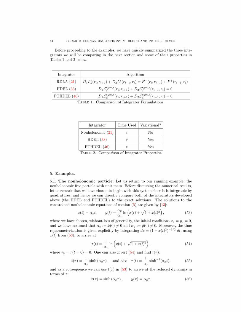
Before proceeding to the examples, we have quickly summarized the three inte-grators we will be comparing in the next section and some of their properties inTables 1 and 2 below.

Integrator Algorithm

RDLA (21) D1L∗d(ri, ri+1) +D2L

∗d(ri−1, ri) = F−(ri, ri+1) + F+(ri−1, ri)

HDEL (33) D1Lsym,εd (ri, ri+1) +D2Lsym,εd (ri−1, ri) = 0

PTHDEL (46) D1Lsym,εd (ri, ri+1) +D2Lsym,εd (ri−1, ri) = 0

Table 1. Comparison of Integrator Formulations.

Integrator Time Used Variational?

Nonholonomic (21) t No

HDEL (33) τ Yes

PTHDEL (46) t Yes

Table 2. Comparison of Integrator Properties.

5. Examples.

5.1. The nonholonomic particle. Let us return to our running example, thenonholonomic free particle with unit mass. Before discussing the numerical results,let us remark that we have chosen to begin with this system since it is integrable byquadratures, and hence we can directly compare both of the integrators developedabove (the HDEL and PTHDEL) to the exact solutions. The solutions to theconstrained nonholonomic equations of motion (5) are given by [13]:

x(t) = αxt, y(t) =αyαx

ln(x(t) +

√1 + x(t)2

), (53)

where we have chosen, without loss of generality, the initial conditions x0 = y0 = 0,and we have assumed that αx := x(0) 6= 0 and αy := y(0) 6= 0. Moreover, the time

reparameterization is given explicitly by integrating dτ = (1 + x(t)2)−1/2 dt, usingx(t) from (53), to arrive at

τ(t) =1

αxln(x(t) +

√1 + x(t)2

), (54)

where τ0 = τ(t = 0) = 0. One can also invert (54) and find t(τ):

t(τ) =1

αxsinh (αxτ) , and also τ(t) =

1

αxsinh−1(αxt), (55)

and as a consequence we can use t(τ) in (53) to arrive at the reduced dynamics interms of τ :

x(τ) = sinh (αxτ) , y(τ) = αyτ. (56)

VARIATIONAL INTEGRATORS FOR HAMILTONIZABLE NONHOLONOMIC SYSTEMS 15

From (56) it follows that

x = sinh

(αxαyy

), (57)

which we will use to compare the performance of the two integrators developedabove.

Let us now turn to the numerical simulations. We have chosen αx = αy = 1,h = hτ = 0.05 and N = 200. Thus, the simulation time hN is 10 seconds. Withour choice of initial conditions the energy E = 1, and we will use the symmetrizedversions of the Lagrangians (28), (52), and (40) with ε = 0.5 as the symmetrizationparameter. Also, since from (54) we see that τ(10) ≈ 2.998, then 200 iterationsin t-time corresponds to τ(10)/hτ ≈ 60 iterations in τ -time. Thus, to more easilycompare the nonholonomic (RDLA) and HDEL integrators, we will choose Nτ = 60.We also wish to note that all of our numerical calculations were done using MAPLE.

Figure 1 below shows a comparison of the root mean square deviation (rmsd) ofthe discrete values computed by each algorithm from the known solutions (53) forthe RDLA and PTHDEL algorithms and (56) for the HDEL algorithm. This error is

defined by√

(xi − x(ti))2 + (yi − y(ti))2 for the RDLA and PTHDEL algorithms,and an analogous expression, with t replaced by τ for the HDEL algorithm. Thermsd error is smallest for the RDLA algorithm (of order 10−4), followed by theHDEL algorithm (of order 10−3) and finally the PTHDEL algorithm (of order 10−2).

(a) (b)

(c)

Figure 1. Nonholonomic Particle: rmsd errors for the (a) RDLA,(b) HDEL, and (c) PTHDEL algorithms.

16 OSCAR E. FERNANDEZ, ANTHONY M. BLOCH AND PETER J. OLVER

The difference of two orders of magnitude in the rmsd errors between the PTHDELand RDLA algorithms is explained by looking at how well they preserve the discreteenergy. Figure 2 (parts (a)-(c)) below shows a comparison of the deviation of thediscrete energies from one for each algorithm. While the RDLA and HDEL algo-rithms both have stable errors of order 10−4 (Figure 2 (a) and (b), respectively),Figure 2(c) shows that the PTHDEL algorithm’s discrete energy values seem togrow linearly away from one. This is expected since, although the PTHDEL al-gorithm results in good long-term behavior for ELc (Figure 2(d)), since (50) here

reads (recall F (r) = (f(r))−1)

Elc(t) = 1 +√

1 + x2ELc ,

as x(t) increases, since ELc remains roughly constant at C ≈ 5.2× 10−4, the t-time

energy Elc(t) − 1 ≈ C√x2(t) = Ct, using (53). Such an increase in the energy

contributes to the rmsd error over the long-term as well (Figure 1(c)).

(a) (b)

(c) (d)

Figure 2. Nonholonomic Particle: deviation from one of the dis-crete energies for the (a) RDLA, (b) HDEL, and (c) PTHDELalgorithms, and (d) deviation from zero of the discrete energy ELcfor the PTHDEL algorithm.

VARIATIONAL INTEGRATORS FOR HAMILTONIZABLE NONHOLONOMIC SYSTEMS 17

Figure 3 shows a comparison of the deviation from zero of each algorithm’sdiscrete constraint values7. The constraint preservation error is smallest for theHDEL algorithm, of order 10−9, followed by the RDLA and PTHDEL algorithms(both of order 10−8).

(a) (b)

(c)

Figure 3. Nonholonomic Particle: constraint errors for the (a)RDLA, (b) HDEL, and (c) PTHDEL algorithms.

Lastly, let us illustrate the application of Proposition 1. From (56), it followsthat F ′′(x(τ)) = cosh(τ). However, as discussed in Remark 1, one would not knowthis before running the HDEL algorithm. Therefore, let us discuss how one can findthe bounds Ci of Proposition 1 using only the numerical results from the HDELalgorithm.

First, we note that from the x Euler-Lagrange equation of Lc, it follows that

x′′ =xx′2

1 + x2. (58)

Then, after finding F ′′(x(τ)) using the chain rule, we can substitute in (58) to arriveat

F ′′(x(τ)) =(x′(τ))2√1 + (x(τ))2

. (59)

7We have constructed this for each of the three integrators by plotting the discretization of theconstraint z + xy, using the exact solution for z and the algorithm solution for x, y.

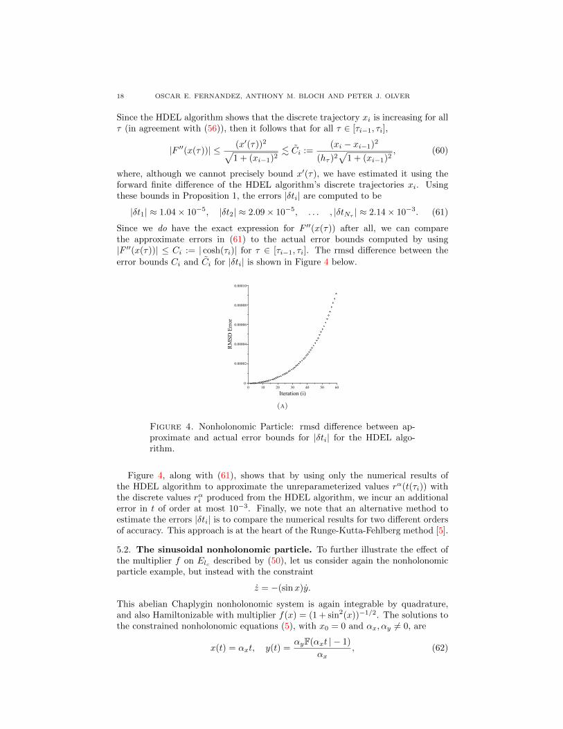
18 OSCAR E. FERNANDEZ, ANTHONY M. BLOCH AND PETER J. OLVER

Since the HDEL algorithm shows that the discrete trajectory xi is increasing for allτ (in agreement with (56)), then it follows that for all τ ∈ [τi−1, τi],

|F ′′(x(τ))| ≤ (x′(τ))2√1 + (xi−1)2

. Ci :=(xi − xi−1)2

(hτ )2√

1 + (xi−1)2, (60)

where, although we cannot precisely bound x′(τ), we have estimated it using theforward finite difference of the HDEL algorithm’s discrete trajectories xi. Usingthese bounds in Proposition 1, the errors |δti| are computed to be

|δt1| ≈ 1.04× 10−5, |δt2| ≈ 2.09× 10−5, . . . , |δtNτ | ≈ 2.14× 10−3. (61)

Since we do have the exact expression for F ′′(x(τ)) after all, we can comparethe approximate errors in (61) to the actual error bounds computed by using|F ′′(x(τ))| ≤ Ci := | cosh(τi)| for τ ∈ [τi−1, τi]. The rmsd difference between the

error bounds Ci and Ci for |δti| is shown in Figure 4 below.

(a)

Figure 4. Nonholonomic Particle: rmsd difference between ap-proximate and actual error bounds for |δti| for the HDEL algo-rithm.

Figure 4, along with (61), shows that by using only the numerical results ofthe HDEL algorithm to approximate the unreparameterized values rα(t(τi)) withthe discrete values rαi produced from the HDEL algorithm, we incur an additionalerror in t of order at most 10−3. Finally, we note that an alternative method toestimate the errors |δti| is to compare the numerical results for two different ordersof accuracy. This approach is at the heart of the Runge-Kutta-Fehlberg method [5].

5.2. The sinusoidal nonholonomic particle. To further illustrate the effect ofthe multiplier f on Elc described by (50), let us consider again the nonholonomicparticle example, but instead with the constraint

z = −(sinx)y.

This abelian Chaplygin nonholonomic system is again integrable by quadrature,and also Hamiltonizable with multiplier f(x) = (1 + sin2(x))−1/2. The solutions tothe constrained nonholonomic equations (5), with x0 = 0 and αx, αy 6= 0, are

x(t) = αxt, y(t) =αyF(αxt | − 1)

αx, (62)

VARIATIONAL INTEGRATORS FOR HAMILTONIZABLE NONHOLONOMIC SYSTEMS 19

where F(t|m) is the elliptic integral of the first kind [30] (Section 19). After Hamil-tonization, the solutions (62) become

x(τ) =1

αxam

(αxτ

αy,−1

), y(τ) = αyτ (63)

in τ -time, where am(τ,m) is the Jacobi amplitude function [30] (Section 22.16).

Because |F (x)| =

∣∣∣∣√1 + sin2(x)

∣∣∣∣ ≤ 2, we expect that the PTHDEL algorithm

will have better long-term energy tracking than in the previous example, since by(50) this would lead to energy errors Elc of roughly the same order as that ofELc . Using the same initial conditions as in the previous example, and again with

ε = 0.5, N = Nτ = 200, h = hτ = 0.5, and the initial energy E = 1, Figure 5(c)below confirms this8. As the figure shows, for the sinusoidal nonholonomic particlesystem all three integrators have comparable long-term energy behavior, with errorsof order 10−4.

(a) (b)

(c) (d)

Figure 5. Sinusoidal Nonholonomic Particle: deviation from oneof the discrete energies for the (a) RDLA, (b) HDEL, and (c)PTHDEL algorithms, and (d) deviation from zero of the discreteenergy ELc for the PTHDEL algorithm.

8In fact, from (50) we can estimate the maximum error in Elc . Using the fact that the maximum

error in ELc is 0.0006 (Figure 5(d)), along with |F | ≤√

2, we estimate that Elc−1 ≤ (0.0006)√

2 ≈0.00085, in agreement with the maximum error in Figure 5(c).

20 OSCAR E. FERNANDEZ, ANTHONY M. BLOCH AND PETER J. OLVER

The corresponding rmsd errors are shown in Figure 6 below. The improvedenergy behavior of the PTHDEL algorithm has led to errors of the same order ofmagnitude as the RDLA algorithm by the end of the computation time (compareFigure 6, parts (a) and (c)). Figure 6(b) shows that the HDEL algorithm has thebest long-term rmsd error behavior of the three algorithms.

(a) (b)

(c)

Figure 6. Sinusoidal Nonholonomic Particle: rmsd error for the(a) RDLA, (b) HDEL, and (c) PTHDEL algorithms.

Finally, Figure 7 below shows a comparison of the deviation from zero of eachalgorithm’s discrete constraint values. Once again the HDEL algorithm producesthe smallest errors (of order 10−9) of the three algorithms (Figure 7(b)). The RDLAand PTHDEL algorithms both have comparable errors of order 10−8 (Figure 7, parts(a) and (c), respectively).

5.3. The knife edge on an inclined plane. Consider a plane slanted at an angleα from the horizontal and let (x, y) denote the position of the point of contact of aknife edge on the plane with respect to a fixed Cartesian coordinate system on theplane, see [1] (Section 1.6). Moreover, let ϕ represent the orientation of the knifeedge with respect to the xy-axis. The Lagrangian and constraints are then givenby

L =1

2

(x2 + y2 + ϕ2

)+ x sinα, y − x tanϕ = 0, (64)

VARIATIONAL INTEGRATORS FOR HAMILTONIZABLE NONHOLONOMIC SYSTEMS 21

(a) (b)

(c)

Figure 7. Sinusoidal Nonholonomic Particle: constraint errors forthe (a) RDLA, (b) HDEL, and (c) PTHDEL algorithms.

where we have set all parameters (mass, moment of inertia, and the gravitationalacceleration) equal to one for simplicity. The system is again Chaplygin Hamil-tonizable with f(ϕ) = cosϕ, [13]. Now, although f has zeros, this will not preventthe application of the results obtained thus far. Indeed, we have that

Lc =1

2(x′2 + cos2 ϕϕ′2) + x sinα.

The reduced equations of motion are once again integrable by quadrature [13],and taking ϕ(0) = x(0) = 0 and ω := ϕ(0) 6= 0 yields the nonholonomic solutions

x(t) =sinα

2ω2sin2(ϕ(t)) +

κ

ωsinϕ(t), ϕ(t) = ωt, (65)

where κ := x(0). The time reparameterization dτ = f(ϕ) dt = cos(ϕ(t)) dt canonce again be integrated explicitly to obtain

τ(t) =1

ωsin(ϕ(t)), (66)

where we have again set τ(t = 0) = 0 for simplicity. We can invert this to obtainthe τ -time version of the solutions (65):

x(τ) =sinα

2τ2 + κτ, ϕ(τ) = arcsin(ωτ), (67)

22 OSCAR E. FERNANDEZ, ANTHONY M. BLOCH AND PETER J. OLVER

where we choose the branch of the inverse sine function based on the values of ϕ(t).Moreover, since (66) shows that |τ(t)| ≤ 1

ω , we conclude that although the solutions

(67) are only defined for τ ∈ [− 1ω ,

1ω ], the change in branch cut for the inverse sine

function as ϕ crosses π2 implies that (67) represents periodic motion, in agreement

with the t-time solutions (65).For our numerical simulations of the knife edge on the inclined plane, we chose

the initial conditions x(0) = ϕ(0) = 0 and κ = ω = 1, and set the incline angleα = 5. We again selected to symmetrize the Lagrangians used, with ε = 0.5, andchose N = 100, h = hτ = 0.07. Thus, our total simulation time in t-time is hN = 7seconds.

Now, since f(ϕ) has roots this means that the corresponding simulation time inτ -time is τ(hN) = τ(7), which is approximately 0.66 seconds, computed from (66).Thus, we have chosen Nτ = N = 100 for the number of iterations in τ -time.

The comparison of the rmsd errors is shown in Figure 8 below. The RDLAalgorithm leads to the smallest rmsd error (of order 10−3), followed by the HDELalgorithm (of order 10−3) and finally the PTHDEL algorithm (of order 10−2). Theabrupt behavior encountered by all the algorithms near iteration numbers i = 23and i = 68 is a result of the fact that ϕ(23h) ≈ π

2 and ϕ(68h) ≈ 3π2 . Near these

values lc, which depends on secϕ, becomes singular. Similarly, since the LagrangiansLc and Lc for the knife edge are

Lc =1

2

(x′2 + (cos2 ϕ)ϕ′2

)+ x sinα

Lc =1

2

((secϕ)x2 + (cosϕ)ϕ2

)+ cosϕ(x sinα+ 1), (68)

near those two iteration points the numerical solver is again attempting to continuethe algorithm despite approaching a singularity (as is the case for Lc, Figure 8(c)),

or approaching a vertical tangent at arcsin(±1) (as is the case for Lc, Figure 8(b)).Figure 9 below shows a comparison of the discrete energy errors for the three

algorithms. The PTHDEL algorithm has the best long-term performance, witherrors of order 10−2 (although these errors increase as the algorithm approachesthe aforementioned iteration values i = 23 and i = 68). The RDLA and HDELalgorithms both have errors of order 10−1. Figure 10 below compares how wellthe three algorithms numerically preserve the nonholonomic constraint. All threealgorithms lead to errors of order 10−9.

6. Conclusion. We have developed two new numerical algorithms to simulatethe mechanics of Chaplygin Hamiltonizable nonholonomic systems, the HDEL andPTHDEL algorithms defined by (33) and (46), respectively. The development ofthese two new integrators was based on the assumption that the underlying non-holonomic system was Chaplygin Hamiltonizable. Although it is certainly not truethat every nonholonomic system is Chaplygin Hamiltonizable, in [2] necessary andsufficient conditions were derived in the form of a coupled set of linear first-orderpartial differential equations for f whose solution, if there is one, determines themultiplier, up to a constant. Practically speaking then, given a nonholonomic sys-tem one can check its Chaplygin Hamiltonizability (using a symbolic software pack-age, like MAPLE), find f , and then apply one of the two integrators developed

VARIATIONAL INTEGRATORS FOR HAMILTONIZABLE NONHOLONOMIC SYSTEMS 23

(a) (b)

(c)

Figure 8. Knife Edge on Inclined Plane: rmsd error for the (a)RDLA, (b) HDEL, and (c) PTHDEL algorithms.

herein. By then exploiting the Hamiltonian form of the time reparameterized re-duced nonholonomic equations, these new algorithms allow the application of vari-ational integrators to non-Hamiltonian nonholonomic systems which are ChaplyginHamiltonizable.

The HDEL algorithm (33) proceeds in the reparameterized time τ , and our nu-merical examples above indicate that it generally leads to superior long-term discreteconstraint preservation behavior relative to the RDLA nonholonomic integrator.The examples also suggest that the long-term discrete energy behavior compareswell with the RDLA algorithm. Moreover, the fact that the HDEL algorithm pro-ceeds in τ -time does not affect its usefulness. As the Example 5.1 showed, for smallenough timesteps h these errors δti can be very small. As an alternative, instead ofinsisting on a smaller timestep to improve this error one can always apply a higher-order quadrature rule to (34) to reduce the error in assigning a discrete t value toeach discrete τ value used in the algorithm.

However, in case one is interested in attempting to preserve the equal timestepsin t-time, a possibility for future research would be to add the holonomic constraintsh =

∫ τi+1

τiF (r(τ)) dτ , i = 1, . . . , Nτ − 1, to the unconstrained Hamiltonian system

defined by the Hamiltonized Lagrangian Lc. By defining the box functions χi,i+1(τ)to be equal to unity for τ ∈ [i, i+ 1] ⊂ [0, N ] and zero otherwise, one could express

24 OSCAR E. FERNANDEZ, ANTHONY M. BLOCH AND PETER J. OLVER

(a) (b)

(c) (d)

Figure 9. Knife Edge on Inclined Plane: deviation from one of thediscrete energies for the (a) RDLA, (b) HDEL, and (c) PTHDELalgorithms, and (d) deviation from zero of the discrete energy ELcfor the PTHDEL algorithm.

these constraints as h =∫ Nτ0

χi,i+1(τ)F (r(τ)) dτ , i = 1, . . . , Nτ − 1. These con-straints then take the form of isoperimetric constraints (see Section 4.3.2 of [33]).One could then apply a holonomic variational integrator, [27], to the new system,and expect the resulting integrator to have roughly fixed timesteps h without theneed (but also without the freedom) of selecting a quadrature rule for (34).

The PTHDEL algorithm, a new application of the Poincare transformation tononholonomic mechanics, also seems to compare well with the RDLA nonholonomicintegrator for multipliers f which are either bounded or show long-term growth. Forthis class of multipliers, the PTHDEL algorithm inherits the favorable long-termdiscrete energy behavior from the variational integrator it is based on. Moreover,as the knife edge example shows, the PTHDEL algorithm may even have superiorlong-term behavior relative to the RDLA integrator for multipliers with roots.

Let us conclude by indicating two more intriguing directions for future research.We note first that despite the requirement that the nonholonomic system underconsideration be Chaplygin Hamiltonizable in order to apply the new integratorsdeveloped here, different techniques exist for the Hamiltonization of nonholonomicsystems [12]. In particular, in [2], Hamiltonization is accomplished by directly

VARIATIONAL INTEGRATORS FOR HAMILTONIZABLE NONHOLONOMIC SYSTEMS 25

(a) (b)

(c)

Figure 10. Knife Edge on Inclined Plane: constraint errors forthe (a) RDLA, (b) HDEL, and (c) PTHDEL algorithms.

solving the inverse problem of the calculus of variations. This method of Hamil-tonization is then used in [29] to simulate the dynamics of a class of nonholonomicsystems using variational integrators. It is within the realm of possibility that onecould combine the results of [2] with the results of [15, ] on Chaplygin Hamil-tonizability to enlarge the class of Hamiltonizable nonholonomic systems. The ideawould be to solve the inverse problem of the calculus of variations for a suitablyreparameterized reduced nonholonomic system, where the reparameterization func-tion f need not be what we have hitherto called the multiplier. As in [2], one wouldexpect a family of Lagrangians as solutions. This freedom to choose the Lagrangiancould be used to develop more accurate and efficient numerical methods for theseHamiltonized systems. In addition, for nonholonomic systems on Lie groups, ananalogous process to Hamiltonization called Poissonization, discussed in [15], couldbe used to develop variational integrators applicable to Poissonizable nonholonomicsystems. A comparison of these results with the works of [11, 20, 28] would beinteresting.

Finally, we wish to mention that although we have restricted ourselves here inbasing the development of our two new integrators on the simplest quadrature rulefor the Lagrangian (13), one could certainly use more advanced quadrature rules as

26 OSCAR E. FERNANDEZ, ANTHONY M. BLOCH AND PETER J. OLVER

a starting point. In particular, the quadrature rules used in the Galerkin Hamil-tonian Variational Integrators and Symplectic Partitioned Runge-Kutta methods,discussed recently in [25], appear to be promising and worth pursuing.

Acknowledgments. The research of OEF was supported by the Institute forMathematics and its Applications through its Postdoctoral Fellowship Program.AMB was supported through NSF grants DMS-0907949, DMS-0806756 and DMS-1207693. PJO was supported through NSF grant DMS-0807317. OEF wouldalso like to thank Alexander Alekseenko and Tom Mestdag for helpful discussionsthroughout the preparation of the paper.

REFERENCES

[1] A. M. Bloch, “Nonholonomic Mechanics and Control,” Interdisciplinary Applied Mathemat-

ics, 24, Systems and Control, Springer-Verlag, New York, 2003.

[2] A. M. Bloch, O. E. Fernandez and T. Mestdag, Hamiltonization of nonholonomic systemsand the inverse problem of the calculus of variations, Rep. Math. Phys., 63 (2009), 225–249.

[3] A. V. Borisov and I. S. Mamaev, Rolling of a rigid body on plane and sphere. Hierarchy ofdynamics, Reg. Chaotic Dyn., 7 (2002), 177–200.

[4] A. V. Borisov and I. S. Mamaev, Conservation laws, hierarchy of dynamics and explicit

integration of nonholonomic systems, Reg. Chaotic Dyn., 13 (2008), 443–490.[5] R. L. Burden and J. D. Faires, “Numerical Analysis,” 8th edition, Thomson Brooks/Cole,

Belmont, CA, 2005.

[6] S. A. Chaplygin, On a ball’s rolling on a horizontal plane, (in Russian), Mat. Sbornik, 24(1903), 139–168; (in English), Reg. Chaotic Dyn., 7 (2002), 131–148.

[7] S. A. Chaplygin, On the theory of motion of nonholonomic systems. The reducing-multiplier

theorem, (in Russian), Mat. Sbornik, 28 (1911), 303–314; (in English), Reg. Chaotic Dyn.,13 (2008), 369–376.

[8] J. Cortes Monforte, “Geometric, Control and Numerical Aspects of Nonholonomic Systems,”

Lecture Notes in Mathematics, 1793, Springer-Verlag, Berlin, 2002.[9] J. Cortes Monforte and S. Martınez, Nonholonomic integrators, Nonlinearity, 14 (2001),

1365–1392.[10] Y. N. Fedorov and B. Jovanovic, Quasi-Chaplygin systems and nonholonomic rigid body

dynamics, Lett. Math. Phys., 76 (2006), 215–230.

[11] Y. N. Fedorov and D. V. Zenkov, Discrete nonholonomic LL systems on Lie Groups, Non-linearity, 18 (2005), 2211–2241.

[12] O. E. Fernandez, “The Hamiltonization of Nonholonomic Systems and its Applications,”

Ph.D. Thesis, The University of Michigan, 2009.[13] O. E. Fernandez and A. M. Bloch, The Weitzenbock connection and time reparameterization

in nonholonomic mechanics, J. Math. Phys., 52 (2011), 012901, 18 pp.

[14] O. E. Fernandez and A. M. Bloch, Equivalence of the dynamics of nonholonomic and vari-ational nonholonomic systems for certain initial data, J. Phys. A, 41 (2008), 344005, 20

pp.

[15] O. E. Fernandez, T. Mestdag and A. M. Bloch, A generalization of Chaplygin’s reducibilitytheorem, Reg. Chaotic Dyn., 14 (2009), 635–655.

[16] P. Fitzpatrick, “Advanced Calculus,” 2nd edition, Thomson Brooks/Cole, Belmont, CA, 2006.

[17] M. R. Flannery, The enigma of nonholonomic constraints, Am. J. of Phys., 73 (2005), 265–272.

[18] Z. Ge and J. E. Marsden, Lie-Poisson Hamilton-Jacobi theory and Lie-Poisson integrators,Phys. Lett. A, 133 (1988), 134–139.

[19] E. Hairer, Variable time step integration with symplectic methods, Appl. Numer. Math., 25(1997), 219–227.

[20] D. Iglesias, J. C. Marrero, D. M. de Diego and E. Martınez, Discrete nonholonomic Lagrangiansystems on Lie groupoids, J. Nonlinear Sci., 18 (2008), 221–276.

[21] M. Kobilarov, J. E. Marsden and G. S. Sukhatme, Geometric discretization of nonholonomicsystems with symmetries, Discrete and Continuous Dynamical Systems, Series S, 3 (2010),61–84.

VARIATIONAL INTEGRATORS FOR HAMILTONIZABLE NONHOLONOMIC SYSTEMS 27

[22] D. Korteweg, Uber eine ziemlich verbreitete unrichtige Behandlungsweise eines Problemesder rollenden Bewegung und insbesondere uber kleine rollende Schwingungen um eine Gle-

ichgewichtslage, Nieuw Archiefvoor Wiskunde, 4 (1899), 130–155.

[23] B. Leimkuhler and S. Reich, “Simulating Hamiltonian Dynamics,” Cambridge Monographson Applied and Computational Mathematics, 14, Cambridge Univ. Press, Cambridge, 2004.

[24] B. Leimkuhler and R. Skeel, Symplectic numerical integrators in constrained Hamiltoniansystems, J. Computational Phys., 112 (1994), 117–125.

[25] M. Leok and J. Zhang, Discrete Hamiltonian variational integrators, IMA J. Numerical Anal-

ysis, 31 (2011), 1497–1532.[26] J. E. Marsden and T. S. Ratiu, “Introduction to Mechanics and Symmetry. A Basic Exposition

of Classical Mechanical Systems,” 2nd edition, Texts in Applied Mathematics, 17, Springer-

Verlag, New York, 1999.[27] J. E. Marsden and M. West, Discrete mechanics and variational integrators, Acta Numerica,

10 (2001), 357–514.

[28] R. McLachlan and M. Perlmutter, Integrators for nonholonomic mechanical systems, J. Non-linear Sci., 16 (2006), 283–328.

[29] T. Mestdag, A. M. Bloch and O. E. Fernandez, Hamiltonization and geometric integration

of nonholonomic mechanical systems, in “Proc. 8 th Nat. Congress on Theor. and AppliedMechanics,” Brussels, Belgium, (2009), 230–236, arXiv:1105.5223.

[30] F. W. J. Olver, D. W. Lozier, R. F. Boisvert and C. W. Clark, eds., “NIST Handbook ofMathematical Functions,” U.S. Department of Commerce, National Institute of Standards

and Technology, Washington, DC; Cambridge Univ. Press, Cambridge, MA, 2010.

[31] T. Ohsawa, O. E. Fernandez, A. M. Bloch and D. V. Zenkov, Nonholonomic Hamilton-Jacobitheory via Chaplygin Hamiltonization, J. Geometry and Phys., 61 (2011), 1263–1291.

[32] J. Ryckaert, G. Ciccotti and H. Berendsen, Numerical integration of the cartesian equations

of motion of a system with constraints: Molecular dynamics of n-alkanes, J. ComputationalPhs., 23 (1977), 327–341.

[33] B. van Brunt, “The Calculus of Variations,” Universitext, Springer-Verlag, New York, 2004.

[34] L. Verlet, Computer experiments on classical fluids, Phys. Rev., 159 (1967), 98–103.

Received May 2011; revised October 2011.

E-mail address: ofernand@wellesley.edu

E-mail address: abloch@umich.edu

E-mail address: olver@umn.edu