Variational inequalities for marketable pollution permits with technological investment...
25
Pergamon M&l. Comput. Modelling Vol. 26, No. 2, pp. l-25, 1997 Copyright@1997 Elaevier Science Ltd Printed in Great Britain. All righta resewed PII: SOS957177(97)00119-Z 08957177/97 $17.00 + 0.00 Variational Inequalities for Marketable Pollution Permits with Technological Investment Opportunities: The Case of Oligopolistic Markets A. NAGURNEY AND K. K. DHANDA* Department of Finance and Operations Management School of Management, University of Massachusetts Amherst, MA 01003, U.S.A. (Received May 1997; accepted June 1997) Abstract-In this paper, we develop a variational inequality framework for the modeling, qualita tive analysis, and computation of equilibrium patterns in multiproduct, multipollutant oligopolistic markets with marketable pollution permits along with opportunities for investment in production technology and/or emission-abatement technology. The model deals explicitly with spatial diieren- tiation and also guarantees that the imposed environmental standards are met through the initial allocation of licenses. An algorithm is proposed, with convergence results, to compute the profit- maximized quantities of oligopoliitic firms’ products and the quantities of emissions, along with the equilibrium allocation of licenses and their prices, ss well ss the optimal investments in the technolo gies. Numerical examples are presented to illustrate the model and the algorithm. Keywords-Environmental policy, Pollution permits, Variational inequalities, Ghgpolistic mar- kets, Technology inveetment. 1. INTRODUCTION Environmental pollution occurs when firms in a region emit pollutants in excess of the amount that can be absorbed by the atmosphere. This is due to the fact that there is no cost attached to the emission of pollutants nor is there any incentive for the reduction of emissions. This problem is further exacerbated since firms are reluctant to invest in technology aimed at the reduction of pollutant emissions. One policy instrument that proposes an incentive to reduce pollution is the marketable permit system, in particular, the ambient-based permit system (APS). In this system, a target level of environment quality is established by the governmental regulatory authority with the level of pollution being defined in terms of total allowable emissions. Subsequently, pollution permits, the entitlement of which would enable the holder to emit a specified amount of pollution, are allocated to the firms. Prom then on, these firms have a choice between reducing emissions through the employment of some emission-abatement technology or by purchasing permits from other emitters holding excess permits in the market. *This research wss supported by a National Science Foundation Faculty Award for Women, NSF Grant No. DMS 9924071.
-
Upload
tien-nguyen -
Category
Education
-
view
37 -
download
0
Transcript of Variational inequalities for marketable pollution permits with technological investment...
Pergamon M&l. Comput. Modelling Vol. 26, No. 2, pp. l-25, 1997
Copyright@1997 Elaevier Science Ltd Printed in Great Britain. All righta resewed
PII: SOS957177(97)00119-Z 08957177/97 $17.00 + 0.00
Variational Inequalities for Marketable Pollution Permits with Technological
Investment Opportunities: The Case of Oligopolistic Markets
A. NAGURNEY AND K. K. DHANDA* Department of Finance and Operations Management School of Management, University of Massachusetts
Amherst, MA 01003, U.S.A.
(Received May 1997; accepted June 1997)
Abstract-In this paper, we develop a variational inequality framework for the modeling, qualita tive analysis, and computation of equilibrium patterns in multiproduct, multipollutant oligopolistic markets with marketable pollution permits along with opportunities for investment in production technology and/or emission-abatement technology. The model deals explicitly with spatial diieren- tiation and also guarantees that the imposed environmental standards are met through the initial allocation of licenses. An algorithm is proposed, with convergence results, to compute the profit- maximized quantities of oligopoliitic firms’ products and the quantities of emissions, along with the equilibrium allocation of licenses and their prices, ss well ss the optimal investments in the technolo gies. Numerical examples are presented to illustrate the model and the algorithm.
Keywords-Environmental policy, Pollution permits, Variational inequalities, Ghgpolistic mar- kets, Technology inveetment.
1. INTRODUCTION
Environmental pollution occurs when firms in a region emit pollutants in excess of the amount
that can be absorbed by the atmosphere. This is due to the fact that there is no cost attached to
the emission of pollutants nor is there any incentive for the reduction of emissions. This problem
is further exacerbated since firms are reluctant to invest in technology aimed at the reduction of
pollutant emissions.
One policy instrument that proposes an incentive to reduce pollution is the marketable permit
system, in particular, the ambient-based permit system (APS). In this system, a target level of
environment quality is established by the governmental regulatory authority with the level of
pollution being defined in terms of total allowable emissions. Subsequently, pollution permits,
the entitlement of which would enable the holder to emit a specified amount of pollution, are
allocated to the firms. Prom then on, these firms have a choice between reducing emissions
through the employment of some emission-abatement technology or by purchasing permits from
other emitters holding excess permits in the market.
*This research wss supported by a National Science Foundation Faculty Award for Women, NSF Grant No. DMS 9924071.

2 A. NAGURNEY AND K. K. DHANDA
The system of marketable pollution permits was given credibility as an economic incentive- based environmental regulation approach to address pollution by Title IV of the 1990 amendments to the Clean Air Act (CAAA). Under Title IV, for example, electric generating facilities can trade allowances or permits for the emissions of sulfur dioxide. In a seminal paper, Montgomery (11 established the theoretical basis of such a system in which the marginal cost of pollution abate- ment is equalized across polluting firms by having them purchase a permit or a license to pollute a prespecified unit of emissions. The regional environmental standards are achieved through the initial allocation of licenses.
The strongest appeal of the economic incentive approach versus the traditional command and control approach is that the former system encourages firms to employ pollution control tech- nologies. For example, a firm participating in a permit market may install emission reducing technologies, lower its level of emissions, and sell the excess entitlements of permits for revenue. Indeed, Burtraw f2] notes that under Title IV, besides allowance/permit trade, a variety of mech- anisms have been employed to achieve compliance. He mentions fuel switching, fuel blending, installing scrubbers, retiring plants, repowering plants, conserving energy, reducing utilization, and substituting among facilities.
There has also been some analysis to determine the incentives to promote technological change. Milliman and Prince [3] explore firm incentives to promote technological change in pollution
control under five regulatory regimes: direct controls, emission subsidies, emission taxes, free marketable permits, and auctioned marketable permits. Their findings suggest that auctioned permits and emission taxes provide the highest firm incentives for technological change. Jung, Krutilla, and Boyd [4] extend the work of Milliman and Prince [3] to analyze pollution abatement technology at an industry level. They compute aggregate profit gain to conclude that auctioned permits provide the maximum incentive for pollution abatement technology.
Previously, the work done by Levin and Reiss [5] analyzed policies for both process and product research and development (R & D). Spence [6] examined problems of appropriability and states that an increase in spillovers would reduce the incentives for a firm to invest in process R & D. De Bondt, Slaets, and Cassiman [7] analyze the interaction between production cost and the cost of innovation for new technology. N&o [S] also explores this linkage and concludes that the cost of production falls as the stock of accumulated knowledge rises. All the previous work has been devoted to product or process R & D aimed at the production process. Magat [9] explored the possibility of R & D funds allocated to two technologies, one aimed at improvement in abatement technology and the other aimed at improvement in production technology.
In this paper, we model multiproduct, multipollutant oligopolistic firms engaged in markets in ambient-based pollution permits. Besides facing production costs and emission costs, the firms also invest in technology aimed at increasing product quantities and at decreasing emission levels. The licenses in excess of initial allocations can be purchased by the firms in order to fulfill the allowance of emissions. If, on the other hand, the firm has met the emissions constraint, it has the option of selling the share of its excess licenses in the market,
We focus on oligopolistic firms, rather than on perfectly-competitive firms, since many of the major polluting generating firms are oligopolistic in their output markets, such as the power plants in the Midwest of the United States, which generate a considerable amount of air pollution. We * sssume further that the firms are perfectly-competitive in the permit markets. More specifically, each source of pollution takes the price of the license to pollute a particular pollutant at a certain point as given, since each source in a region is small relative to the entire economy. The model also deals explicitly with spatial differentiation through the use of a diffusion matrix that maps emissions from sources to receptor points that are dispersed in space.
In order to remain competitive both in the short run and the long run, a firm needs to update the level of technology employed that is aimed at improving its production process. Whereas, some large firms can choose to invest in research and development (R & D) devoted to the innovation of new technology or to invest in the improvement of existing technology, some smaller firms

Variational Inequalities 3
may have the option of purchasing the new improved technology in the market. The employment
of improved technology would result in more efficient production processes that yield increased levels of production. But in the presence of regulatory controls, for example, in the case of environmental emission limits, the firms need to incorporate technology that would also comply
with the regulatory controls set by the regulatory agency. Besides striving for a higher production
output, the firms need to contain the levels of pollutants emitted. In a market-based system such as Title IV of the 1990 CAAA, the development of emissions-abatement technology is encouraged since the firms that succeed in lowering the levels of emissions have the option to sell the excess entitlements of permits for revenue.
The mathematical framework that is chosen for the formulation, qualitative analysis, and com- putation of the equilibrium pattern in markets for pollution control in the presence of investment in technology is that of finite-dimensional variational inequality theory. Hecently, variational inequality theory has been used in environmental economic policy modeling in the context of ambient-based pollution permit markets in oligopolistic markets but only in the case of single product, single pollutant oligopolistic firms, and in the absence of technology costs (cf. [lo]). Hence, this paper extends the earlier work to a more general setting with the inclusion of produc- tion enhancing technology and emission-abatement technology. Moreover, we emphasize that, to-date, no general computational procedure or model has been developed to handle technology choices in such a setting.
For a plethora of additional equilibrium problems in both economics and operations research that have been studied as variational inequality problems, see the book by Nagurney [ll].
Our model applies the theory of variational inequalities to yield the profit-maximized quantities of multiple products, the optimal quantities of the various emissions, the optimal investments in production technology and in emission-abatement technology, the equilibrium allocation of the pollution licenses, and the prices of the licenses. We aim to make a contribution in the direction of environmental economics since the use of variational inequality theory to this field has yet to be fully explored.
The paper is organized as follows. In Section 2, we develop the optimization problem faced by the individual firm in the presence of investment in technology. Subsequently, we present the economic conditions governing the market model and then derive the variational inequality formulation of the equilibrium conditions. In addition, we also provide the qualitative properties of the equilibrium pattern. In Section 3, we propose an algorithm for the computation of the equilibrium pattern and provide conditions for convergence. This algorithm yields variational inequality subproblems of very simple structure, each of which can then be solved explicitly and in closed form. This algorithm is then applied to compute solutions to several numerical examples in Section 4 of increasing complexity. Last, we summarize our results and present conclusions in Section 5.
2. THE MARKET MODEL WITH INVESTMENTS IN TECHNOLOGY
In this section, we develop the multiproduct, multipollutant market model with ambient-baaed pollution permits in which the firms can invest in resources to improve the production technology and/or the emission-abatement technology. As environmental standards get more stringent, the tail-end solutions to reduce emissions, such as the installation of scrubbers, may not remain feasi- ble. The firms that intend to remain competitive in the long run may need to invest in resources in order to incorporate production technology along with the emission abatement technology to improve the production possibilities and to reduce the emissions simultaneously.
We consider m sources of industrial pollution in the region, which are fixed in location, with a typical source denoted by i. There are n receptor points, with a typical receptor point denoted by j. Also, let there be T different pollutants emitted by the sources, with a typical pollutant

4 A. NAGURNEY AND K. K. DHANDA
denoted by t. Let et denote the amount of pollutant t emitted by firm i and group the firm’s emissions into a vector ei E R’,. We group then all the firms’ emissions into the vector e E Ry .
We assume, as given, an r x m x n diffusion matrix H, where the component ht denotes the contribution that one unit of emission by source i makes to average pollutant concentration of type t at receptor point j. Montgomery [l] proposed the idea that the emissions vector ei can be mapped into concentrations by the diffusion matrix so that the resultant emissions do not exceed the externally set standard. Here, we prove this result in our more general model.
Let a permit denote a license, the possession of which will allow a source to pollute a specific pollutant at some specific receptor point. Each polluter, hence, will have to hold a portfolio
of licenses to cover all of the relevant monitored receptor points. Let It denote the number of licenses for pollutant t at point j held by source i and group the licenses for each firm i into a vector li E R3f. We assume throughout that some initial allocation of licenses 18; i = 1,. . . , m; j = l,..., 7-b; t = l,..., r, has been made by the regulatory agency and we group this initial
allocation of licenses into a vector 1: E R 3’. We then further group all the licenses of the firms
into the vector 1 E R;tnr. Furthermore, let pi denote the price of the license for pollutant t that affects receptor point j
and group the prices of the licenses into the vector p E RI;n. Also, assume that the market in pollution licenses is perfectly competitive, that is, each source of pollution takes the price of the license to pollute at a specific point as given and cannot affect the price itself, since each source is small relative to the entire economy.
Let there be s distinct products that are produced by the firms in a noncooperative manner, with a typical output denoted by d and the quantity of product d produced by firm i denoted by Qid. These quantities are first grouped into the vector qi E R$ and then further into the
ms vector q E R+ . Each of the products is assumed to be homogeneous, that is, the consumers are indifferent as to which firm wss the producer.
It is essential for the firms that aim to be competitive in the long run to invest in resources devoted to incorporating new technologies or to improving the presently employed technologies. Let Aid denote the investment of resources, for example, dollars, by firm i to improve its pro duction possibilities for the product d. Group the firm’s investment in production technologies into a vector Ai E R$_. Further group all the firms such investments into the vector A E RI;“. Similarly, let Bit denote the investment of resources by firm i to improve its emission-abatement technologies aimed at the reduction of emissions level for pollutant t. Group the firm’s invest- ment in emission-abatement technologies into a vector Bi E R’+ and all such investments of all the firms into the vector B E RT.
The basic idea behind the market in pollution permits is that firms or sources of pollution must be encouraged to trade permits. A typical firm participating in a permit market has to take into account various costs, such as the cost of production, the cost of emission-abatement, the cost of purchasing pollution licenses, and, finally, the costs involved in the adoption of technology, both for production and emission-abatement purposes.
Each firm i in the oligopoly is faced with a cost _fi of producing the vector of quantities qi, where
.fi = fi(qi, Ai), (1)
that is, this cost is dependent upon the vector of quantities produced by the firm and the amount of investment in production technology employed by the firm.
Each firm i in the region is faced with a cost Gi of emitting the vector of emissions ei, where
Gi = Gi(ei,qi, Bi). (2)
This cost is dependent upon the vector of emissions, the vector of production quantities, and the amount of investment in emission-abatement technology employed by the firm.

Variational Inequalities 5
Since we assume that the firms are oligopolistic in their output markets, they affect the prices of their outputs. Hence, if we denote the price of product d by pd, we can write
(3)
Consequently, each firm i acquires a revenue of
Since the regulatory body bestows upon the firm i a portfolio of an initial allocation of li- censes 1:, the value of a firm’s initial endowment of licenses is given by C&r Cc1 $I$, where $ denotes the given price of a license to pollute for the specific pollutant t at receptor point j, which, under the assumption of perfect competition in the license markets, is assumed given.
Also, the cost of purchasing licenses for a specific pollutant t that affects receptor point j for source i is given by
n
(5) j=l
We assume that each firm in the oligopoly is profit-maximizing and, thus, can be characterized by a utility function that measures its profit or net revenue. The utility function ui faced by each such firm i; i = 1,. . . , m, can, hence, be expressed as the difference between total revenue acquired and the total cost incurred by the firm:
- G(ei, Qi, Bi) - c Aid - c Bi - c c # (it _ $) . d=l t=1 t=l j=l
An oligopolistic firm’s optimization problem is then expressed as
Maximize ui (q,ei,Ai,&,li) 7
subject to: ht.& <I?. rj 1 - 83 7 t=1,.*., T, j=l,..., n,
(7)
(8)
and the normegativity constraints
Qid 1 0, ht.et Qr- > 0 1 htjA+d 2 0, htB,” L 0, ht$. ij *, - > 0 9 d = 1,. . . s,
, hijt=l,...,r, h$= l,...,n. (9)
Constraint (8) states that each firm is allowed to have an average rate of emission that produces no more pollution at any point than the amount which the firm is licensed to cause at that point.
Let Xzj denote the Lagrange multiplier associated with the tjth constraint, and let Xi denote the vector of Lagrange multipliers in Rqn. Finally, group the vectors Xi into the vector X E RTm. Note that Xt may be interpreted as a shadow price and, henceforth, we term this Lagrange multiplier as the marginal abatement cost.
As stated earlier, the oligopolistic firms are assumed to operate in a noncooperative manner in their product markets, where the governing equilibrium concept is that of Nash-Cournot, and is defined as follows.

6 A. NAGURNEY AND K. K. DHANDA
DEFINITION 1. NASH EQUILIBRIUM. A Nash equilibrium is a vector of production outputs q* E q, emission quantities e* E R;_“, production technology investments A* E Ry , emission- abatement technology investments B’ E R;t’, and licenses 1’ E Rqmn, such that
ui q~,~~,e~,Af,Bf,lf (
) 2 ui (qi,P;‘,ei,Ai,Bi,li),
Vqi E Rd,, Vei E R;, VAi E R$, VBi E R’,, Vii E Rl;T, (10)
satisfying (8) and (9) for all firms i, where i; = (q;, . . . ,ql_l,qi;l,. . . ,q&).
In other words, the rationality postulate here is that each firm selects its production outputs so
that its utility is maximized, given the production output vector decisions of other oligopolistic
firms, and also its emissions, its investment in production and emission-abatement technology,
and licenses.
Optimality Condition for a Firm
If we assume that the utility function ui(q, ei, Ai, Bi, ii), for each firm i is concave with respect
to its arguments, and is continuously differentiable, the necessary and suEcient conditions for
an optimal firm-specific product, emission, investment in production technology, investment in
emission-abatement technology, license, and marginal abatement cost pattern
(qz,ez,Af,Bf,I;,Xt),
given (~9) is that this pattern is nonnegative and satisfies the inequality
+ G(eT,qf,Bf) _ @d(cz19;)
%id &id q;d - pd x kid - &I
n + C XiTht
j=l 1 x [et - et*]
1 X [Aid - &] + 1 1 x [Bit - B:*]
(11)
t=l j=l t=l j=l
vqid 2 0, et 2 0, Aid 2 0, B; 2 0, 16 2 0, X~j 2 0,
d= l,...,s, j=l n, ,***, t = l,...,T.
Note that a similar inequality needs to hold for each of the other oligopolistic firms (see also,
e.g., [W.
Market Clearing Conditions for Licenses
We now describe the system of equalities and inequalities governing the quantities and prices
of licenses in the region at equilibrium. Mathematically, the economic system conditions governing market clearance in pollution per-
mits are: for each pollutant t; t = 1,. . . , r, and for each receptor point j; j = 1, . . . , n:
~0, ifpt*>O g [I:.? - “‘;I { > 0 - 1 if i* _ 0 3-’
02)
The system (12) states that: if the price of a license for pollutant t at a point j is positive,
then the market for licenses at that point must clear; if there is an excess supply of licensee for a
particular pollutant t at a receptor point, then the price of a license at that point must be zero.

Variational Inequalities 7
DEFINITION 2. MARKET EQUILIBRIUM. A vector of production outputs, emissions, production, and emission-abatement technology, licenses, associated marginal costs of abatement, and license
prices (**, e*, A*, B’, I*, X*,p*) E R2738+27?W+2WWI+m
is an equilibrium point of the multiproduct, multipollutant oligopoly with ambient-based pollu-
tion permits developed above if and only if it satisfies inequality (11) for alI firms i = 1, . . . , m, and the system of equalities and inequalities (22) for all receptor points: j = 1, . . . , TZ, and for all
pollutants: t = 1,. . . , r.
We now derive the variational inequality formulation of the equilibrium conditions for the above
market model.
THEOREM 1. A vector of firm production outputs, emissions, production, and emission-abate- ment technology investments, licenses, and associated shadow prices,
(**, e*, A’, B’, 1’) ),*, p*) E R2mS+2mr+2Tmn+Tn
is an equilibrium point if and only if it satisfies the variational inequality problem
afi (qt, 4) + G (et7 !& B,‘) aPd cc:, &d>
hid a&d - hid x hid - ‘$d]
n + C Xi;ht x [ei - eF*]
j=l 1 X [Aid - A$]
+eiI i=l t=1
+E i=l d=l
+22 i=l t=1
+3 i=l t=1
+c t=1 j=l
(13)
aGi ($%&f& Bf) + 11 x [BE _ Bi”*]
*
n r n
C [py - Ai;] X [Zij - l$] + C C [IiT - hte:‘] x [Xij - AiT] j=l t=l j=l
V (q, e, A, B, 1, X,p) E R~ms+2mr+2rmn+m.
PROOF. Assume that (q’, e*, A*, B’, I’, X*,p*) E R2ma+2mr+2rmn+m is an equilibrium. Note that inequality (11) holds for all firms i = 1, . . . , m. Hence, summing (11) over all firms, we
obtain
+ 2 f: [ afifiidAT) + 11 x [Aid - AH] i=l d=l
aGi (et,q;, B;) aB;
+ 1 1 x [B; - Bf*]
(14

8 A. NAGURNEY AND K. K. DHANDA
+ 2 2 g [I:; - hijet’] X [Xtj - $1 2 0, *cl fix1 j=l
V (q, e, A, B, 1, X) E R$ms+2mr+2mn.
Also, from the system (12), we can conclude that the equilibrium must satisfy
(14) (cont.)
(15)
Finally, summing (14) and (15), one obtains variational inequality (13).
We now establish the converse of the proof, that is the solution to (13) also satisfies (11)
and (12).
Let (q*,e*,A*,B*,l*,X*,p*) E R 2ms+2mr+2mn+m be a solution of (13). If one lets Qjd = &,
for all i, d; eF = e:“, for ah i, t; Aid = A* id, for all i, d; Bit = B:*, for all i, t; It = l$, for all i, j, t;
At = A$, for ail i, j, t, and substitutes these values into (13), one obtains
which implies the system-conditions (12).
Similarly, if one lets pi = p? for all j, t, and substitutes these values into (13), one obtains
afi k&A;) + aGi (ef,t,W _ %'d cc:, q;cf> aqid @id a&d
&d - L’d x [%d - &]
aGi (e;, qz, Bf) ae:
+ 2 Xi;hij j=l 1 x [e: - ey]
+ 2 f: [ afi!$;dAt’ + 11 X [Aid - Ard]
i=l drl (17)
i=l t=l j=l
+ 2 2 2 [It; - hijef+] X [Xij - ~tj*] 2 0, +l t=l j=l
V (q, e, A, B, I, X) E R:!s+2mr+2rmn,
which implies that (11) must hold for ail the firms. The proof is complete.
We now put variationsl inequality (13) into standard form (cf. 1111). Define the column vector
X E (q, e, A, B, X, p) E R~me+2mr+2rmn+m and F(X) as the row vector consisting of the row vec-
tors: (G(X), E(X), o(X), P(X), L(X), h(X), J’(X)), w h ere G(X) is the ms-dimensional vector with component id given by -2, E(X) is the mr-dimensional vector with component it given by
-$$+& Xijhij, a(X) is the ms-dimensional vector with component id given by ,w+l,
p(X) is the nar-dimensional vector with component it given by v + 1, L(X) is the
Variational Inequalities 9
mnr-dimensional vector with component ijt given by pi - At, A(X) is the mnr-dimensional vector with component ijt given by It - hte:, and P(X) is the m--dimensional vector with jtth component given by C%,(I$’ - 1ij).
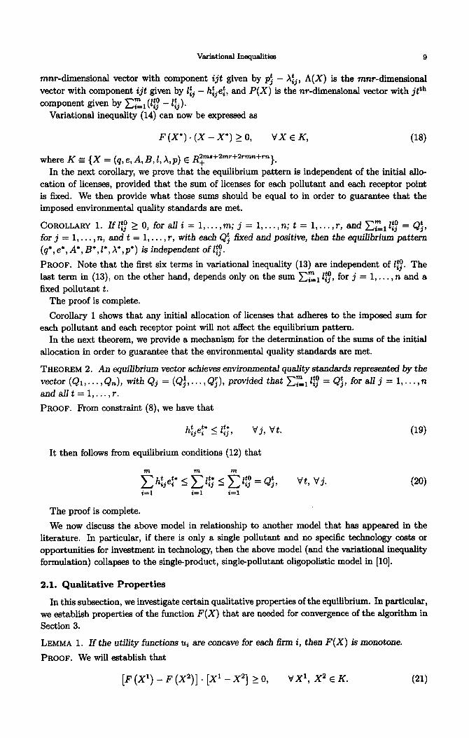
Variational inequality (14) can now be expressed as
F (x*) * (X - x*) 2 0, VXEK, (18)
where K c (X = (q, e, A, B, 1, X,p) E R~!a+2mr+2tmn+cn}. In the next corollary, we prove that the equilibrium pattern is independent of the initial allo-
cation of licenses, provided that the sum of licenses for each pollutant and each receptor point is fixed. We then provide what those sums should be equal to in order to guarantee that the imposed environmental quality standards are met.
COROLLARY 1. If1$‘> 0, foralli = l,..., m; j = l,..., n; t = l,..., T, and C&Z:! = Q$, forj=l,..., n,andt=l,..., r, with each Qi fixed and positive, then the equilibrium pattern (q’, e*, A*, B*, I*, X*,p*) is independent of l$‘.
PROOF. Note that the first six terms in variational inequality (13) are independent of 1:;. The last term in (13), on the other hand, depends only on the sum CL, l$‘, for j = 1,. . . , n and a fixed pollutant t.
The proof is complete.
Corollary 1 shows that any initial allocation of licenses that adheres to the imposed sum for each pollutant and each receptor point will not affect the equilibrium pattern.
In the next theorem, we provide a mechanism for the determination of the sums of the initial allocation in order to guarantee that the environmental quality standards are met.
THEOREM 2. An equilibrium vector achieves environmental quality standards represented by the
vector (QI,. . . , Qn), with Qj = (Q),..., Q:), provided that Czll$ = Qj, ford j = l,...,n
andallt=l,...,r.
PROOF. From constraint (8), we have that
Vj, Vt. (19)
It then follows from equilibrium conditions (12) that
The proof is complete.
We now discuss the above model in relationship to another model that has appeared in the literature. In particular, if there is only a single pollutant and no specific technology costs or opportunities for investment in technology, then the above model (and the variational inequality formulation) collapses to the single-product, single-pollutant oligopolistic model in [lo].
2.1. Qualitative Properties
In this subsection, we investigate certain qualitative properties of the equilibrium. In particular, we establish properties of the function F(X) that are needed for convergence of the algorithm in Section 3.
LEMMA 1. If the utility functions ui are concave for each firm i, then F(X) is monotone.
PROOF. We will establish that
[F (Xl) -F (X2)] . [X1 -X2] > 0, VX’, X2 E K. (21)

10 A. NAGURNFX AND K. K. DHANDA
In view of the definition of F(X) in the above model, (21) takes the form
azLi (q’,et,Af,B,‘,Zf ) hi (q2, ef, A:, Bf, 1:) hid - hid I x [dd - q?d]
(22)
i=l t=l j=l
+ 2 g 2 (1;; - 1;;) - (I;; - z$) x [pjl -#I . t=l j=l 1 i=l 1
After combining and simplifying terms, the expression (22) reduces to
(23)
aGi (ef, qf’, Bf)
aB; x [B:’ - Bi2] .
But under the assumption that the utility functions are concave, we know that minus the gradient of the utility function is monotone (cf. [ll]) and, hence, the expression in (23) must be greater than or equal to zero. The proof is complete.
LEMMA 2. The function F(X) is Lipschitz continuous, that is, there exists a positive constant L,
such that IIF (xi) - F (x2) I] I L [[xi - x2]] , vxl, x2 E K, (24)
under the assumption that the utility functions have bounded second-order derivatives.
PROOF. Follows from the same arguments as the proof of [ll, Lemma 8.11. We now provide an existence result, but first recall the definition of coercivity.
DEFINITION 3. A function F(z), from a feasible set K to Rn is said to be coercive, if
w - ; y,, ,; (2 - 4 --t o. X Xl
, (25)
as llxll + 00 for z E K, and for some x1 E K.
Variational Inequa.lities 11
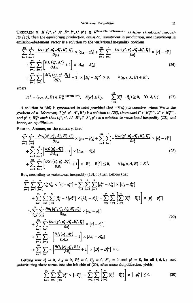
THEOREM 3. If (q’, e*, A*, B' , I*, A’, p*) E R2ms+2mr+2rmn+m satisfies variational inequal- ity (13), then the equilibrium production, emission, investment in production, and investment in
emission-abatement vector is a solution to the variational inequality problem
*
ICC &,(q*,ef,Af,Bz,If)
&d x Iqid _ qrdl + 2 2 _hi (q*,e;eCBf,If) x [e: - er]
i=l d=l i=l kl t
+ 2 f: [ ahfi;dAf) + 11 x [Aid - A;] i=l d=l
+ee[ aGi (er q’ B;)
i=l t=1
&;’ +I] x [B:-B,“*] 20, V(q,e,A,B)EK’, ,
(26)
where
K1 = (q, e, A, B) E RT+2rmn+m, hijet < It, F(l:;” - l&) 2 0, Vi, d, t, j. (27) i=l
A solution to (26) is guaranteed to exist provided that -Vu(.) is coercive, where Vu is the gradient of u. Moreover, if (q’, e*, A*, B’) is a solution to (26), there exist I’ E RI;““, X* E Rkrnn, andp* E R’+” such that (q*,e*,A*,B*,l*,X*,p*) is a solution to variational inequality (13), and
hence, an equilibrium.
PROOF. Assume, on the contrary, that
ICE ’ azl,(q*,ef,At,Bf,If) - @id
x [qid _ q;j + 2 2 _ &i (Cl*? “teff 3 Bf9 Cl x [e: _ e;*]
i=l d=l i=l t=1 I
+ 2 2 [ afit)dAf) + I] X [Aid - Azd]
i=l d=l
aGi (et, q!, Br) aBi
+ 1 1 x [B; - B;*] 5 0, V (q, e, A, B) E K’.
(28)
But, according to variational inequality (13), it then follows that
~~~X~;h~jX [e: - eF*] + 2 2 2 [py - $1 X [lij - 1$] i=l t=1 j=l is1 t=1 jE1
i=l t=1 j=l
222 L&(q*,ef,Ai,B,*,lf)
i=l d=l &id X
+Fk azli(q*,ey,Af,Bt,Zt)
i=l t=1 ae:
t=1 j=l Liz1 J
[‘&d - !$dl
x [ei - ep]
(29)
m s
+cc- i=l d=l m +
i=l t=1
Letting now e: =
ah (q:> 4) aAid
+ 1 I X [Aid - A;d]
dGi (et,@, Bf)
dBi + 1 1 x [Bt” - B;*] 2 0.
0, Aid = 0, B: = 0, It = 0, X~j = 0, and p; = 0, for all t, d, i, j, and
substituting these terms into the left-side of (29), after some simplification, yields
(30)

12 A. NACWRNEY AND K. K. DHANDA
Thus, we have established a contradiction to (28). Therefore, variational inequality (26) must be satisfied.
Moreover, under the coercivity condition on -Vu, the existence of a solution to (26) is guar- anteed from the standard theory of variational inequalities (cf. [ll]). Finally, according to the Lagrange Multiplier Theorem, there exist nonnegative multipliers X’ and p’ corresponding to the linear equality constraints in K’, which must satisfy (13). The proof is complete.
Note that a coercivity condition on the utility functions of the firms in an oligopolistic market was also imposed by Gabay and Moulin [12] in order to obtain an existence result.
3. THE ALGORITHM
In thii section, we present an algorithm for the solution of variational inequality (18), equiv- alently (13), governing the market equilibrium model for pollution permits in the presence of technological investment opportunities. The algorithm resolves the variational inequality prob- lem into very simple subproblems, each of which can be solved explicitly and in closed form.
The algorithm that we propose for the computation of the equilibrium pattern is the modified projection method of [13]. The algorithm is guaranteed to converge, provided that F satisfies only the monotonicity condition and the Lipschitz continuity condition, assuming that a solution exists.
The statement of the modified projection method is as follows.
STEP 0. INITIALIZATION. Set X0 E K. Let ,L!l = 1 and let a be a scalar such that 0 < a < l/L, where L is the Lipschitz continuity constant (cf. (24)).
STEP 1. COMPUTATION. Compute Xp by solving the variational inequality subproblem
[ Xfl + CxF (X@-l)T - x+1] T * [x - q 2 0, for all X E K.
STEP 2. ADAPTATION. Compute Xp by solving the variational inequality subproblem
(31)
[ X@ + aF (P)’ - x+1] T * [x - x0] 10, for all X E K. (32)
STEP’ 3. CONVERGENCE VERIFICATION. If max ]X/ - Xf-‘] 5 c, for all I, with E > 0, a prespecified tolerance, then stop; else, set p = p + 1, and go to Step 1.
For completeness, we now state the above algorithm in which F(X) is in expanded form for our specific model.
STEP 0. INITIALIZATION. Set (q”, e”, A”,Bo, lo, X”,po) E R~m6+2mr+2rmn+m. Let p = 1 ad
set a so that 0 < (Y < l/L.
STEP 1. COMPUTATION. Compute (@, d, @, BP, la, Ao,$) E Rtm6+2mr+2nnn+nr by solving the variational inequality subproblem
(33)

Variational Inequalities 13
V (q, e, A, B, I, X, p) E R~ms+2mr+2rmn+m.
STEP 2. ADAPTATION. Compute (qp, e@, AP, BP, lp, Xp,$) E R~ms+2mr+2rmn+nr by solving the variational inequality subproblem
(34)
V (q, e, A, B, 1, X, p) E R~ms+2mr+2rmn+m,
STEP 3. CONVERGENCE VERIFICATION. If maxid Iq$ - qf,-'l 5 E; maxit Ie:” - ei’-‘I I e;
maxid IA& -A$‘1 _ < E; maxit IBf - Bf-l I 5 c; mwjt Ilk - l$’ I 5 e; maxijt /.A$ - .A$-’ I 5 e;
majt I$ - p7-l I 5 E; for all i, j, d, t, with e > 0, a prespecified tolerance, then stop; else, set p = p + 1, and go to Step 1.
We now discuss the modified projection method more fully. We first recall the definition of the projection of z, on the closed convex set, K, with respect to the Euclidean norm, and denoted
by PKX, as
y = PKx = mzfmmn llz - zll. (35)
In particular, we note that, (cf. [ll, Theorem 1.21) xfl generated by the modified projection method as the solution to the variational inequality subproblem (31) is actually the projection

14 A. NAGURNEY AND K. K. DHANDA
of (XP-’ - aF(X fl-‘)T) on the closed convex set K, where K here is simply the nonnegative orthant. In other words,
P ZPK [ Xp-1 - crF (xP-1) ‘1 . (36)
Similarly, Xfl generated by the solution to variational inequality subproblem (32) is the projection of x+’ - ~#(a~)~ on the nonnegative orthant, that is,
x0 = PK [x0- - CYF (X@)‘] . (37)
Since, the feasible set here is of box type, the above projections immediately decompose across the coordinates of the feasible set. In fact, the solution of each of the variables encountered in (33) and (34) amounts to projecting onto R+ separately.
Consequently, we can provide closed-form expressions for the solution of problems (33) and (34). In particular, we have that (33) can be solved as follows.
For all firms i; i = 1, . . . , m, and all products d; d = 1,. . . , s, set
and for firms i; i = l,..., m, and all pollutants t; t = 1,. . . , T,
I$” = msx aui qp-1, ,$-l, A?l, BP-‘, if-l n 0 I
ae: c X%‘h?. $3
j=l
Forallfirmsi;i=l,..., m,andaIlproductsd;d=l,..., s,set
For all firms i; i = 1, . . . , m, and all pollutants t; t = 1,. . . , T, set
- G (ef-‘, qf-‘, Bfel) _ 1
aBi
(38)
(39)
(40)
(41)
For all firms i; i = 1, . . . , m, all receptor points j; j = 1,. . . , n, and all pollutants t; t = 1,. . . , r,
set
and
Finally, for all receptor points j; j = 1,. . . , n, and all pollutants t; t = 1,. . . , r, set
Variational inequality subproblem (34) can be solved explicitly in closed form in a similar manner.
Convergence is given in the following.
THEOREM 2. The modifkd projection method described above converges to the solution of vari- ational inequality (18) under the assumptions that the utility functions have bounded second order derivatives and are concave.
PROOF. It follows from Lemmas 1 and 2 that the function F(X) is both monotone and Lips&& continuous, under the stated assumptions. Hence, as established in [13, Theorem 21, the modiied projection method is guaranteed to converge under these conditions.

Variational InequaIities 15
4. NUMERICAL EXAMPLES
In this section, we present numerical examples illustrating the model presented in Section 2,
along with the performance of the algorithm of Section 3.
We present five examples of increasing complexity. All the examples have quadratic production
cost and emission cost functions.
Each firm i in each example faces a production cost function of the form
(45)
with the specific terms for the parameters reported along with the examples.
The demand price function for product d in each example was given by
(46)
Each firm i in each example also faced an emission cost function of the form
(47)
with the specific terms for the parameters reported along with the examples.
The initial allocation of the licenses, the I@, were set as 1:; = 1, for all i, j,t, The difbrsion
matrix H terms, the ht’s were set as follows. For t = 1: h$ = l.(i/j), if i <= j; and hij =
0.5(i/j), otherwise, for all i, j. For t = 2: hij = 2(i/j), if i C= j; and ht = O.l(i/j), otherwise,
for all i, j. The initial values for the quantities were set as follows: & = 30, if i <= d; and qFd = 50,
otherwise. The initial values for the emissions were set as follows: ef = 20, for all i, t. The initial
values for the investment in production enhancing technology were set as follows: AL = 15, for
all i, d. The initial values for the investment in emission abatement technology emissions were
set as follows: B: = 5, for all i, t.
All other initial variables were initialized to 1.
The convergence tolerance E was set to 0.0001 and the parameter o was set to 0.1 in the
algorithm for all the examples.
The algorithm was coded in FORTRAN 77. The system used was the IBM SP2 located at the
Cornell Theory Center at Cornell University. In addition to the number of iterations required for
convergence of the modified projection method, we also report the CPU time, exclusive of input
and output and setup times.
Finally, for each example, we also provide the following information, the total investment in
production technology for all firms, which is denoted by TA, and is given by
TA = 2 f: Aid, (43) i=l dzl
as well as the total investment in emission-abatement technology, which is denoted by TB, and
is given by
TB = 2 &. (49) i=l t=l
EXAMPLE 1. In this example, the oligopoly consisted of two firms that produce two outputs and
emit two pollutants, which, in turn, affect two receptor points. Refer to Table 1 for the production

16 A. NAGURNEY AND K. K. DHANDA
Table 1. Example l-production co& and technology invwtment parameters.
Firllli 4hl 442 422il F&2 4% +3i2 Of1 C2fl
1 0.12 0.18 8.0 3.0 2.0 5.0 1.0 4.0 2 0.15 0.20 6.0 3.0 4.0 7.0 2.0 1.0
Table 2. Example l-emission cost and technology inve8tment p8mme-tere.
cost and production technology investment parameters and to Table 2 for the emission cost and emission technology investment parameters. In this example, as well ss in all of the subsequent ones, we set Cla = 0.01 and 71: = 0.01 for all i,d,t.
The algorithm converged in 29938 iterations and 2.30 seconds of CPU time and yielded the equilibrium production vector for Firms 1 and 2, respectively,
q; = (45.406,41.196),
q; = (41.599,37.175),
the equilibrium emission vector for Firms 1 and 2, respectively,
e; = (4.000,1.051),
e; = (0.000,9.490),
the equilibrium investment in production enhancing technology vector for Firms 1 and 2, respeo
tively,
A; = (0.000,149.996),
A; = (49.999,0.000),
the equilibrium investment in emission reducing technology vector for Firms 1 and 2, respectively,
B; = (0.000,49.999),
B; = (149.996,99.998),
the equilibrium licenses for Firms 1 and 2, respectively,
1” 11 = 2.000, 6:; = 0.104, 1:; - - 2 . 000 , z:; = 1.051,
1;; = 0.000, 1;; = 1.897, 1;; = 0.090, 1;; = 0.949,
the equilibrium marginal costs of abatement for Firms 1 and 2, respectively,
A” 11 = 36.630, A:; = 92.763, Xi; = 27.370, A:; = 24.673,
Xii = 26.348, A$ = 92.763, A$; = 17.862, Xg = 24.673,
and the equilibrium prices for licenses affecting receptor point 1 and receptor point 2, respectively,
Pi’ = 36.630, py = 92.763,
P; = 27.370, pr = 24.673.
Variational Inequalities 17
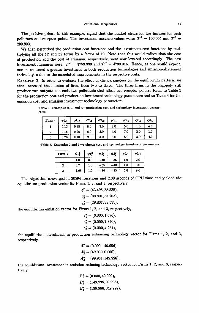
The positive prices, in this example, signal that the market clear8 for the licenses for each
pollutant and receptor point. The investment measure value8 were: TA = 199.995 and TB = 299.993.
We then perturbed the production co8t, functions and the investment cost function8 by mul-
tiplying all the 62 and q2 terms by a factor of 10. Note that this would reflect that the cost
of production and the cost, of emission, respectively, were now lowered accordingly. The new
investment measure8 were: T A = 3799.939 and TB = 4799.916. Hence, as one would expect,
one encountered a greater investment in both production technologies and emission-abatement
technologies due to the associated improvements in the respective costs.
EXAMPLE 2. In order to evaluate the effect of the parameters on the equilibrium pattern, we
then increased the number of firm8 from two to three. The three firm8 in the oligopoly still
produce two outputs and emit, two pollutant8 that affect two receptor points. Refer to Table 3
for the production cost and production investment technology parameter8 and to Table 4 for the
emission cost and emission investment technology parameters.
Table 3. Examples 2, 3, and 4-production cost and technology investment param- eters.
Table 4. Examples 2 and 3-emission cc& and technology investment parameters.
The algorithm converged in 20594 iterations and 2.30 seconds of CPU time and yielded the
equilibrium production vector for Firm8 1, 2, and 3, respectively,
q; = (43.495,38.535),
q; = (38.801,33.203),
q; = (29.837,38.535),
the equilibrium emission vector for Firm8 1, 2, and 3, respectively,
e; = (6.000,1.576),
e; = (0.000,7.840),
eg = (0.000,4.261),
the equilibrium investment in production enhancing technology vector for Firm8 1, 2, and 3,
respectively,
A; = (0.000,149.996),
A; = (49.999,0.000),
A; = (99.981,149.996),
the equilibrium investment in emission reducing technology vector for Firm8 1, 2, and 3, respec-
tively,
B; = (0.000,49.999),
B; = (149.996,99.998),
B; = (199.996,349.992),

18 A. NAGURNEYAND K.K. DHANDA
the equilibrium licenses for Firm 1:
1;; = 3 * 000 , 1;; = 0 * 158 , 1:; = 3.000,
the equilibrium licenses for Firm 2:
1;; = 0 * 000 I 1;; = 1 * 567 t 1;; = 0.000,
the equilibrium licenses for Firm 3:
1;; = 0 * 000 I 1;; = 1 * 277 , 1;; - -* 0 000 ,
and the equilibrium marginal costs of abatement for Firm 1:
Xii = 33 * 569 I X3; = 110.401, xi; = 22 * 431 ,
and the equilibrium marginal costs of abatement for Firm 2:
Xii = 26.376, Gi = 110.401, A;; = 17.673,
and the equilibrium marginal costs of abatement for Firm 3:
Xii = 15.998, Ai; = 110.401, A;; = 8.940,
1:; = 1 * 576 ,
1;; = 0 * 784 f
1,“; = 0 * 639 ,
x:; = 22 * 384 9
A;; = 22.384,
Af; = 22.384,
and the price vector for licenses afIecting receptor point 1, receptor point 2, and receptor point 3,
respectively,
p;‘ = 33.569, pT* = 110.401,
pi* = 22.431, pi* = 22.384.
Note, that in this example, the markets in licenses for each pollutant and receptor point also
cleared and, hence, the prices were positive.
The investment measure values were: TA = 449.990 and TB = 849.982. Since there are more
participants in the permit market, the investment measure for both production and emission-
abatement technologies increased.
We then conducted the same type of simulation as in Example 1 by perturbing the <2’s and 772’s
by a factor of 10. The new investment measure values were: TA = 7199.878 and T* = 11199.794.
Hence, as one would expect, one encountered a greater investment in both production technologies
and emission-abatement technologies due to the associated improvements in the respective costs.
EXAMPLE 3. In order to evaluate the effect of the parameters on the equilibrium pattern, we
then increased the number of receptor points from two to three. The three Gms in the oligopoly still produce two outputs and emit two pollutants. Refer to Table 3 for the production cost and
production investment technology parameters and to Table 4 for the emission cost and emission
investment technology parameters.
The algorithm converged in 18294 iterations and 2.42 seconds of CPU time and yielded the
equilibrium production vector for Firms 1, 2, and 3, respectively,
q; = (43.495,38.535),
q; = (38.801,33.203),
q; = (29.837,38.535),

Variationel Inequalities 19
the equilibrium emission vector for Firms 1, 2, and 3, respectively,
e; = (6.000,1.578),
e; = (0.000, .789),
eg = (0.000,8.945),
the equilibrium investment in production enhancing technology vector for Firms 1, 2, and 3,
respectively,
A; = (0.000,149.996),
A; = (49.991,0.000),
A; = (99.998,149.996),
the equilibrium investment in emission reducing technology vector for Firms 1, 2, and 3, respec-
tively,
Bi = (0.000,49.991),
B; = (149.996,99.981),
B; = (199.996,349.992),
the equilibrium licenses for Firm 1:
1:; = 3 * 000 , 1:; - -* 0 157 , 1;; = 3 * 000 > 1;; = 1 - 577 > 1:; = 2 - 305 9 1:; = 1 * 051 9
the equilibrium licenses for Firm 2:
2:: = 0 * 000 , I,“; = 0 * 157 , 1:; = 0 * 000 , 1;; = 0.079, I;; = 0 * 274 , 1;; - -* 1 052 3
the equilibrium licenses for Firm 3:
1;; = 0 * 000 9 1,“; = 2.688, 1;; = 0 * 000 7 1;; = 1 * 344 , 1;; = 0 * 217 7 1;; = 0 * 896 9
and the equilibrium marginal costs of abatement for Firm 1:
A;; = 32 - 438 7 x:; = 77 * 513 , A;; = 23 * 562 9
A:; = 14 * 960 , x;; = 0 * 000 ? A:; = 16 * 083 I
and the equilibrium marginal costs of abatement for Firm 2:
A;; = 26 * 765 , x;; = 77 * 513 , A;; = 16 ’ 503 ?
A;; = 14.960, A& = 0 * 000 , A;; = 16 * 083 >
and the equilibrium marginal costs of abatement for Firm 3:
A;; = 15.636, xi; = 77 * 513 , A;; = 8 * 737 ,
A;; = 14 * 960 , A& = 0 * 217 9 A;; - - 16 ’ 083 9
and the price vector for licenses affecting receptor point 1, receptor point 2, and receptor point 3,
respectively,
pi* = 32.438, p:’ = 77.413,
Pli = 23.562, pp = 14.960,
pi* = 0.000, pi* = 16.083.

20 A. NACURNEY AND K. K. DHANDA
Note, that in this example, the markets in licenses for each pollutant and receptor point also cleared, and hence, the prices were positive.
The investment measure values were T A = 449.990 and TB = 849.982. We note that the investment measure for both production and emission-abatement technologies remains the same as in the last example. This leads us to conclude that a change in the number of receptor points in the permit market does not directly impact the investment measures for a firm, at least in this particular example.
We then changed the [2 and 712 terms in the same manner ss in the preceding two examples. The new investment measure values were: TA = 7199.878 and TB = 11199.794. Hence, as one would expect, one encountered a greater investment in both production technologies and emission-abatement technologies due to the associated improvements in the respective costs but, as stated above, this measure is the same as the one in the previous example.
EXAMPLE 4. In order to evaluate the effect of the parameters on the equilibrium pattern, we now increased the number of pollutants from two to three. The three firms in the oligopoly still produce two outputs and emit pollutants that affect three receptor points. Refer to Table 3 for the production cost and production investment technology parameters and to Table 5 for the emission cost and emission investment technology parameters.
Table 5. Examples 4 and 5-emission cost and technology investment parameters.
The algorithm converged in 18294 iterations and 3.15 seconds of CPU time and yielded the equilibrium production vector for Firms 1, 2 and 3, respectively,
Qi = (43.495,38.535),
q; = (38.801,33.203),
q; = (29.837,38.535),
the equilibrium emission vector for Firms 1, 2, and 3, respectively,
ei = (6.000,1.577,20.000),
e; = (0.000,0.789,25.000),
eg = (0.000,8.962,17.647),
the equilibrium investment in production enhancing technology vector for Firms 1, 2, and 3, respectively,
Af = (0.000,149.996),
A; = (49.999,0.000),
A; = (99.998,149.996),
the equilibrium investment in emission reducing technology vector for Firms 1, 2, and 3, respec- tively,
Bi = (0.000,49.999,99.998),
B; = (149.996,99.998,149.996),
B; = (199.996,349.992,249.996),
Variational Inequalities 21
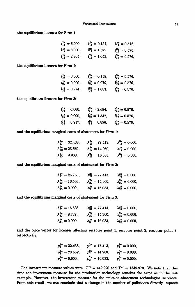
the equilibrium licenses for Firm 1:
1” 11 = 3.000,
11’1 = 3.000,
1:; = 2.305,
the equilibrium licenses for Firm 2:
1” 21 = o.ooo,
1;; = 0.000,
1” 23 = 0.274,
the equilibrium licenses for Firm 3:
1;; = 0.000,
1;; = 0 - 000 ,
l& = 0 * 217 ,
12’ 11 = 0.157,
12’ 12 = 1.579,
1:; = 1053 * ,
1;; = 0 - 158 ,
1;; = 0 * 079 ,
1;; = 1 * 053 ,
I;; = 2.684,
13: = 1.342,
1% = 0.896,
z3* 11 = 0.576,
1;; = 0.576,
1:; = 0 * 576 9
cr = 0.576,
1;; = 0.576,
1:; = 0.576,
1,“; = 0.576,
1;; = 0.576,
1;; = 0 - 576 ,
and the equilibrium marginal costs of abatement for Firm 1:
A:; = 32.438, A:; = 77 413 * , A;; = 0.000,
A;; = 23.562, x:; = 14 960 * 3 x;; = 0 000 * 9
x:; =oooo * , A:; = 16.083, x:; = 0.000,
and the equilibrium marginal costs of abatement for Firm 2:
+A:; = 26.765, Ai; - 77 413 - * , A:; = 0 000 * ,
A;; = 16 503 * , A;; = 14 960 * 9 xi; = 0.000,
x;; - 0 000 -* 7 x2* 23 = 16.083, x;; = 0.000,
and the equilibrium marginal costs of abatement for Firm 3:
Xii = 15 636 * , X3; = 77.413, XSjf = 0 000 * ,
A;; = 8 737 * , A;; = 14.960, xi; = 0 000 - ,
x;; = 0.000, A;; = 16 083 * 9 xi; = 0 000 * ,
and the price vector for licenses affecting receptor point 1, receptor point 2, receptor point 3, respectively,
Pi’ = 32.438, pp = 77.413, pp = 0.000,
pp = 23.562, pp = 14.960, p? = 0.000,
pi* = 0.000, p;’ = 16.083, p? = 0.000.
The investment measure values were: TA = 449.990 and TB = 1349.973. We note that thii time the investment measure for the production technology remains the same as in the last example. However, the investment measure for the emission-abatement technologies increases. From this result, we can conclude that a change in the number of pollutants directly impacts
22 A. NAGURNFX AND K. K. DHANDA
the investment measures in emission-abatement technology but it does not directly impact the investment measures in production technology.
We then increased the CZ terms and the 772 terms in the same manner as in the preceding example simulations. Recall that such a change reflects a reduction in the production and emission cost functions. The new investment measure values were T* = 7199.878 and TB = 17549.674. Hence, as one would expect, one encountered a greater investment in both production technologies and emission-abatement technologies due to the associated improvements in the respective costs.
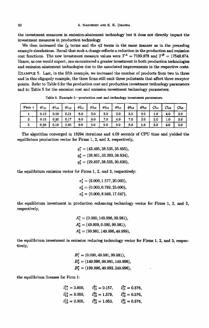
EXAMPLE 5. Last, in the fifth example, we increased the number of products from two to three and in this oligopoly example, the three firms still emit three pollutants that affect three receptor points. Refer to Table 6 for the production cost and production investment technology parameters and to Table 5 for the emission cost and emission investment technology parameters.
Table 6. Example 5-production cost and technology investment parameters.
Firm i 4161 4liZ 4li3 4‘41 &i2 &i3 @il &i2 43i3 @iI C2i2 C2t3
1 0.12 0.18 0.21 8.0 3.0 5.0 2.0 5.0 3.0 1.0 4.0 3.0
2 0.15 0.20 0.17 6.0 3.0 7.0 4.0 7.0 2.0 2.0 1.0 3.0
3 0.20 0.18 0.30 9.0 3.0 5.0 3.0 5.0 1.0 3.0 4.0 2.0
The algorithm converged in 18294 iterations and 4.09 seconds of CPU time and yielded the equilibrium production vector for Firms 1, 2, and 3, respectively,
q; = (43.495,38.535,35.855),
q; = (38.801,33.203,38.834),
q; = (29.837,38.535,30.836),
the equilibrium emission vector for Firms 1, 2, and 3, respectively:
e; = (6.000,1.577,20.000),
e; = (0.000,0.789,25.000),
eZJ = (0.000,8.948,17.647),
the equilibrium investment in production enhancing technology vector for Firms 1, 2, and 3, respectively,
A; = (0.000,149.996,99.981),
A; = (49.999,0.000,99.981),
A; = (99.981,149.996,49.999),
the equilibrium investment in emission reducing technology vector for Firms 1, 2, and 3, respec- tively,
B; = (0.000,49.991,99.981),
B; = (149.996,99.981,149.996),
B3+ = (199.996,49.992,249.996),
the equilibrium licenses for Firm 1:
1;; = 3 * 000 , 1;; - -* 0 157 7 1;; = 0.576,
z:; = 3.000, 12’ 12 = 1.579, 1;; = 0.576,
I;; = 2.305, 1:; = 1.053, 1% = 0.576,

Variational Inequalities
the equilibrium licenses for Firm 2:
23
1;; = 0 * 000 9 I!;; = 0.158, 1,“; = 0.576,
1:; = 0 * 000 I 1;; - -* 0 079 , 1;; = 0.576,
1;; = 0.274, 1;; = 1.053, 1:; = 0.576,
the equilibrium licenses for Firm 3:
Gi = 0.000, 1:; = 2.684, 1,“; = 0 * 576 ?
1;; = 0 * 000 7 1;; = 1 * 342 , 1;; = 0.576,
1;; = 0 * 217 > 1;; = 0 * 895 9 1;; = 0 * 576 9
and the equilibrium marginal costs of abatement for Firm 1:
Xii = 32 * 438 I Xfi = 77.413, ATi = 0 * 000 ,
A;; = 23 ’ 562 3 A;; = 14 * 960 > x;; = 0 * 000 ,
xi; = 0.000, A:; = 16.083, A:; = 0.000,
and the equilibrium marginal costs of abatement for Firm 2:
Ai; = 26.765, XX; = 77.413, Ai; = 0.000,
A;; = 16 * 503 > A;; = 14 - 960 I xx; = 0.000,
x;; = 0.000, A;; = 16 * 083 9 xx; = 0.000,
and the equilibrium marginal costs of abatement for Firm 3:
Ai; = 15 * 636 9 A$ = 77 * 413 9 A,“; = 0 * 000 ,
xi; = 8.737, A;; = 14.960, xi; = 0 * 000 3
xi; = 0 * 000 9 A;; = 16.083, A;; = 0 * 000 ,
aud the price vector for licenses affecting receptor point 1, receptor point 2, receptor point 3, respectively,
pi* = 32.438, p:* = 77.413, pp = 0.000,
p;* = 23.562, pp = 14.958, pp = 0.000,
p? = 0.000, p? = 16.083, pp = 0.000.
The investment measure values were TA = 699.985 and TB = 1349.973. We note that this time the investment measure for emission-abatement technology remains the same as in the last example. However, the investment measure for production technology increases. From this result we can conclude that a change in the number of products directly impacts the investment measures in production technology but it does not impact the investment measure in emission- abatement technology. We then changed the c2 and 72 values as in the preceding examples by increasing them by a factor of 10. The new investment meaSure values were TA = 11049.802 and TB = 17549.674. Hence, as one would expect, one encountered a greater investment in both production technologies and emission-abatement technologies due to the associated improvements in the respective costs.
24 A. NAGURNEY AND K. K. DHANDA
These examples illustrate the effect of the various parameters, such as the number of firms, products, receptor points, pollutants, and changes in investment cost parameters, on the invest- ment measures for production and emission-abatement technology. Specifically, we note that a decrease in the investment costs led to an increased measure of investment. Furthermore, the investment measures for both production and emission-abatement technology are most signifi- cantly impacted by the number of firms participating in the permit market. Also, the investment measure for production technology is affected by the number of products and the investment measure for emission abatement technology is affected by the number of pollutants.
The above numerical examples highlight the variety of multiproduct, multipollutant oligopoly problems with marketable pollution permits that can be solved in the presence of investment opportunities in both production technologies and emission-abatement technologies. Although the algorithm requires a large number of iterations for convergence, each iteration of the algorithm is remarkably simple and computationally very efficient since closed form expressions are used. Moreover, the computed solutions are very accurate.
5. SUMMARY AND CONCLUSIONS
In this paper, we have presented a variational inequality framework for the formulation, qualita- tive analysis, and computation of equilibria in multiproduct, multipollutant oligopolistic markets with marketable pollution permits and with opportunities for investment in technology. In par- ticular, two kinds of technology are considered-production enhancing technology and emission- abatement technology. The model significantly extends those that have been presented in the literature to-date.
Also, we proposed an algorithm, the modified projection method, along with convergence results. In the context of the model developed here, the algorithm resolves the equilibrium problems into very simple subproblems, which can then be solved explicitly and in closed form. Finally, to illustrate both the model and the algorithm, we presented several numerical examples to provide both insight into the model as well as the performance of the algorithm.
Additional research in the future will include the modeling of noncompliant firms, that is, firms that emit pollutants above that allowed by their permit holdings, ss well as the incorporation of dynamics into the models developed by us thus far.
REFERENCES 1. W.D. Montgomery, Markets in licensee and efficient pollution control programs, Jounurl of Economic Theory
5, 395-418, (1972). 2. D. Burtraw, The SO2 emissions trading program: Co& savings without allowance trades, Contemponarg
Economic Pokey 2, 79-94, (1996). 3. S. Millii and R. Prince, Firm incentives to promote technological change in pollution control, Journal of
Environmental Economics and Management 17, 247-265, (1989). 4. C. Jung, K. Krutilla and R. Boyd, Incentives for advanced pollution abatement technology at the industry
level: An evaluation of policy alternatives, Journal of Environmental Economics and Management SO, 95- 111, (1978).
5. R.C. Levin and P.C. Reii, Cc&-reducing and demand-creating R & D with spillovers, RAND Journal of Economics 10, 538-556, (1988).
6. M. Spence, Cost reduction, competition, and industry performance, Econometrica 52, 101-121, (1984). 7. R. De Bond& P. Slaets and B. Caaeiman, The degrw of epillm and the number of rivala for maximum
effective R & D, International Joumal of Industrial Organization 10,35-54, (1992). 8. T. Nakao, Co&reducing R&D in oligopoly, Journal of Economic Behavior and Organization 12, 131-48,
(1989). 9. W. Magat, Pollution control and technological advance: A dynamic model of the tlrm, Journal of Envtmn-
mental Economics and Management 5, l-25, (1996). 10. A. Nagurney and K. Dhanda, A variational inequality approach for marketable pollution permits, Computa-
tional Economics 0, 360-384, (1996). 11. A. Nagurney, Network Economics: A Variational Inequality Approach, Kluwer Academic Publishers, Boston,
MA, (1993).

Variational Inequalities 25
12. D. Gabay and I-I. Mouh, On the uniqueness and stability of Nash equilibria in noncooperative games, In Applied Stochohic Control in Econometrica and Management Science, (Edited by A. Bensousean, P.S. Kleindorfer and C.S. ‘I&&o), North-Holland, Amsterdam, The Netherlands, (1980).
13. G.M. Korpekvich, The extragradient method for finding saddle pointa and other problems, Matekon 13, 35-49, (1977).