Submitted byMario Gobrial

Submitted atInstitute ofComputationalMathematics

SupervisorO.Univ.-Prof. Dipl.-Ing.Dr. Ulrich Langer

Co-SupervisorDr. Ioannis Toulopoulos

August 2020

JOHANNES KEPLERUNIVERSITY LINZAltenbergerstraße 694040 Linz, Osterreichwww.jku.atDVR 0093696

Variational Inequalitiesand Their Finite ElementDiscretization

Master Thesis

to obtain the academic degree of

Diplom-Ingenieur

in the Master’s Program

Industriemathematik

Abstract

Contact problems are quite frequently phenomena occurring in mechanical applications. Itquickly turned out that variational inequalities are an appropriate tool to precisely characterizecontact problems. Unfortunately, variational inequalities involve a lot of computational diffi-culties when solving them numerically. Over the past years, a large amount of methods forthe numerical computation of variational inequalities has been developed. Depending on thetype and complexity of the contact problem, different kinds of variational inequalities have beenevolved. The Signorini problem is a famous contact problem describing the touching between anelastic body and a rigid frictionless foundation. However, frictional contact exhibit in realisticproblems. Thus, the investigations of the classical Signorini problem expanded to the exam-ination of the Signorini problem with so-called Coulomb friction. This thesis introduces theclassical frictionless Signorini problem, and we will derive its variational inequality. We deeplyanalyze abstract variational inequalities, distinguishing between inequalities derived from mini-mization problems and general inequalities, where the question about the existence of a uniquesolution will be answered for both cases. As an extension, we analyze hemi-variational inequali-ties, which are associated with frictional contact problems. The Finite Element discretization issubsequently considered for both types of inequalities, variational and hemi-variational, wherethe convergence of the approximate solutions is investigated. Additionally, we obtain theoreti-cal error estimates, which are finally verified with the outcomes of numerical examples for thesimplified Signorini problem and the obstacle problem.

I

Zusammenfassung

Kontaktprobleme sind haufig auftretende Phanomene in mechanischen Anwendungen. Es stell-te sich schnell heraus, dass variationelle Ungleichungen ein geeignetes Hilfsmittel fur die genaueCharakterisierung von Kontaktproblemen darstellen. Unglucklicherweise treten bei der nume-rischen Berechnung von variationallen Ungleichungen viele Schwierigkeiten auf. In den letztenJahren hat sich eine große Anzahl an Methoden fur die numerische Berechnung von varia-tionellen Ungleichungen entwickelt. Unterschiedliche Arten von variationellen Ungleichungenentstanden in Abhangigkeit vom Typ und der Komplexitat des Kontaktproblems. Das Signo-rini Problem ist ein bekanntes Kontaktproblem, dass den Kontakt zwischen einem elastischenKorper und einem staaren reibungslosen Fundament beschreibt. Allerdings tritt Reibung inrealistischen Problemen haufig auf, sodass die Forschung des Singorini Problems sich auf dieUntersuchung des Signorini Problems mit sogenannter Coulombscher Reibung erweiterte. Indieser Arbeit wird das klassische reibungslose Signorini Problem eingefuhrt und dessen va-riationelle Ungleichung hergeleitet. Es werden abstrakte variationelle Ungleichungen vertieftanalysiert. Dabei unterscheidet man variationelle Ungleichungen, die von Minimierungsproble-men abgeleitet werden und allgemeine Ungleichungen. In beiden Fallen wird die Frage uberdie Existenz einer eindeutigen Losung beantwortet. Desweiteren werden hemi-variationelle Un-gleichungen analysiert, die mit reibungsbehafteten Kontaktproblemen in Verbindnung gebrachtwerden. Die Finite Elemente Diskretisierung von beiden Ungleichungstypen, sowohl variationelals auch hemi-variationel, wird betrachtet und die Konvergenz von Naherungslosungen wird un-tersucht. Zusatzlich werden theoretische Fehlerschatzer hergeleitet, die schließlich anhand vonErgebnissen numerischer Beispiele fur das vereinfachte Signorini Problem und das HindernisProblem verifiziert werden.

II

Acknowledgments

First, I would like to extend my sincere thanks to my supervisor Prof. Dip.-Ing. Dr. UlrichLanger for the scientific discussions, for the continuous guidance and for providing me a placeat the Institute of Computational Mathematics to write this thesis.

I would like to emphasize my deepest gratitude to Prof. Dipl.-Ing. Dr. Andreas Pauschitz,the general director of AC2T research GmbH, Austrian Center of Tribology, for the financialsupport of this thesis and for giving me the opportunity to be a part of valuable discussionswith other great members of AC2T research GmbH, especially DI. Dr.techn. Georg Vorlauferand Dipl.-Ing.(FH) Stefan Krenn, MSc.

I would also like to express my special thanks to my co-supervisor Dr. Ioannis Toulopoulosfor introducing me this topic, the scientific guidance, and the encouragement and support forthis work. I appreciate his effort, the cooperation and his valuable time for proofreading thethesis.

In addition, I would like to thank Prof. Dipl.-Ing. Dr Walter Zulehner for his valuable timeand annotations for this work.

Finally, I want to express my sincerest appreciation and thanks to my family for supportingme endlessly all the time and to my friends for their encouragement and the enjoyable timeover the last years.

This work was supported by the project COMET K2 InTribology 872176, partly carried outat ”Excellence Center of Tribology” AC2T research GmbH, 2700 Wiener Neustadt, Austria.

Mario GobrialLinz, August 2020

III

Contents

1 Introduction 1

2 Preliminaries 32.1 Notations . . . . . . . . . . . . . . . . . . . . . . . . . . . . . . . . . . . . . . . 32.2 Function spaces . . . . . . . . . . . . . . . . . . . . . . . . . . . . . . . . . . . . 52.3 Important theorems . . . . . . . . . . . . . . . . . . . . . . . . . . . . . . . . . . 7

3 Linear Elasticity 93.1 Eulerian and Lagrangian coordinates and deformation . . . . . . . . . . . . . . . 93.2 Displacement, velocity and acceleration . . . . . . . . . . . . . . . . . . . . . . . 113.3 Strain tensor . . . . . . . . . . . . . . . . . . . . . . . . . . . . . . . . . . . . . 123.4 Forces and stresses . . . . . . . . . . . . . . . . . . . . . . . . . . . . . . . . . . 133.5 Conservation laws . . . . . . . . . . . . . . . . . . . . . . . . . . . . . . . . . . . 15

3.5.1 Conservation of mass . . . . . . . . . . . . . . . . . . . . . . . . . . . . . 153.5.2 Conservation of linear momentum . . . . . . . . . . . . . . . . . . . . . . 163.5.3 Equilibrium equation . . . . . . . . . . . . . . . . . . . . . . . . . . . . . 173.5.4 Conservation of angular momentum . . . . . . . . . . . . . . . . . . . . . 17

3.6 Constitutive laws . . . . . . . . . . . . . . . . . . . . . . . . . . . . . . . . . . . 17

4 Signorini and Obstacle Problem 194.1 Classical Signorini problem . . . . . . . . . . . . . . . . . . . . . . . . . . . . . . 19

4.1.1 Linearized contact conditions . . . . . . . . . . . . . . . . . . . . . . . . 204.1.2 Classical form . . . . . . . . . . . . . . . . . . . . . . . . . . . . . . . . . 244.1.3 Variational form . . . . . . . . . . . . . . . . . . . . . . . . . . . . . . . 25

4.2 Simplified Signorini problem . . . . . . . . . . . . . . . . . . . . . . . . . . . . . 294.3 Obstacle problem . . . . . . . . . . . . . . . . . . . . . . . . . . . . . . . . . . . 33

5 Analysis of Variational Inequalities 345.1 Introductory examples . . . . . . . . . . . . . . . . . . . . . . . . . . . . . . . . 345.2 Variational inequalities in Rd . . . . . . . . . . . . . . . . . . . . . . . . . . . . . 355.3 Elliptic variational inequalities in Hilbert spaces . . . . . . . . . . . . . . . . . . 38

5.3.1 Minimization problems of elliptic variational inequalities . . . . . . . . . 395.3.2 Existence and uniqueness results of variational inequalities . . . . . . . . 44

5.4 Elliptic hemi-variational inequalities . . . . . . . . . . . . . . . . . . . . . . . . . 505.4.1 Application of hemi-variational inequalities: Contact problems with Coulomb

friction . . . . . . . . . . . . . . . . . . . . . . . . . . . . . . . . . . . . . 54

6 Finite Element Discretization 606.1 Discretization of elliptic variational inequalities . . . . . . . . . . . . . . . . . . 606.2 Discretization of elliptic hemi-variational inequalities . . . . . . . . . . . . . . . 68

IV

7 Numerical results 747.1 Numerical results for the obstacle problem . . . . . . . . . . . . . . . . . . . . . 74

7.1.1 Dual methods . . . . . . . . . . . . . . . . . . . . . . . . . . . . . . . . . 757.1.2 Penalty methods . . . . . . . . . . . . . . . . . . . . . . . . . . . . . . . 78

7.2 Numerical results for the simplified Signorini problem . . . . . . . . . . . . . . . 827.3 A more realistic example . . . . . . . . . . . . . . . . . . . . . . . . . . . . . . . 83

8 Conclusion and Outlook 878.1 Conclusion . . . . . . . . . . . . . . . . . . . . . . . . . . . . . . . . . . . . . . . 878.2 Outlook . . . . . . . . . . . . . . . . . . . . . . . . . . . . . . . . . . . . . . . . 88

Bibliography 91

V

Chapter 1

Introduction

In the early nineteenth century, many engineers, physicists and mathematicians have started arigorous investigation about contact problems of solid bodies after the establishment of the fun-damental principles of continuum mechanics. In fact, the first treatment with deformable bodieshas been considered within the framework of continuum mechanics and was later transferredto problems involving contact. Surprisingly, there is no consistent definition of the contact.However, many people describe the contact of two bodies as the touching of the surface of thetwo bodies at a certain time. The first successful contribution about contact problems in elas-ticity, where a linear elastic body comes in touch with a rigid and frictionless foundation, wasachieved by A. Signorini towards the end of the 1950s. Some years later, his student G. Ficheracontinued the examination on Signorini’s problem and represented the first result about theexistence and uniqueness of a solution for variational inequalities arising from minimization offunctionals on convex subsets of Banach spaces. He named this type of contact problem afterhis teacher as an honor, calling it the Signorini problem. Fichera’s work was the starting pointfor many scientific researchers to indulge in deep analysis of abstract variational inequalities,which are not necessarily related to minimization problems. However, variational inequalitiesare often connected to problems defined on convex sets. Hence, the convexity is an essentialproperty for deducing some special results. In 1967, J. Lions and G. Stampacchia [44] publishedastonishing results about the theory of variational inequalities, followed by G. Duvaut and J.Lions [9] in 1972, associating variational inequalities with mechanical applications. After thesecontributions, many other works from prestigious authors of this area as K. Atkinson and W.Han [1], D. Kinderlehrer and G. Stampacchia [19], R. Glowinski [13], R. Glowinski, J. Lions andR. Tremolieres [14] and N. Kikuchi and T. Oden [18], to name just a few, have been presented.

Contact problems are inherently nonlinear, such that many difficulties must be dealt withwhen solving the mathematical problem numerically. Over the past years it turned out thatvariational inequalities are the most effective mathematical models to describe and solve con-tact problems, since they appropriately handle the conditions and restrictions on the contactboundary. Nowadays, contact problems are immediately associated with variational inequalitiesand conversely. Additionally, a wide range of numerical methods for computing approximatesolutions of variational inequalities have been developed and many different techniques areprovided depending on the structure and level of difficulty of the variational form.

Although the Signorini problem covers various applications of contact problems, there isstill a large amount of problems, which require different descriptions. The classical Signoriniproblem involves the contact of an elastic body with a rigid frictionless foundation. However,frictional contact problems are a frequently discussed topic in mechanical applications, butcause severe difficulties during the computation of solutions. The first investigations of contactproblem with dry friction are due to G. Duvaut and J. Lions [9], where the contact of an elasticbody with a rigid foundation was considered. In the literature, such problems are usually called

1

Signorini problem with Coulomb friction, since the physical friction laws are derived from thephysician C. Coulomb. Frictional problems require more general observations of variationalinequalities, so-called quasi- or hemi-variational inequalities. These type of inequalities involveenormous mathematical complications, where some of them have not been resolved until now.Important first results in this direction have been published by J. Necas, J. Jarusek, J. Haslinger[46]. This release opened the door for many other researchers to deeply study the theory offrictional contact problems and their related quasi- or hemi-variational inequalities. Somerelevant publications are published by J.T. Oden and E. Pires [48], L. Demkowicz and J.T.Oden [33] and M. Cocu [32], to name just a few. The contributions by K. Atkinson andW. Han [1], R. Glowinski [13], R. Glowinski, J.L. Lions, R. Tremolieres [14], N. Kikuchi andT. Oden [18], I. Hlavacek, J. Haslinger, J.Necas, J. Lovısek [16], P.D. Panagiotopoulos [24],A.R. Capatina, M. Cocu [31] and A. Capatina, M. Cocou, M. Raous [30] about the numericalapproximations of variational and hemi-variational inequalities highly enriched the theory offrictional contact problems. Recent results about the approximation of variational inequalitieswere obtained by A. Capatina [6], W. Han [34], S. Migorski, S. Zeng [45], R. Krause [41], R.Krause and B. Wohlmuth [43] and W. Han, M. Sofonea [35].

The motivation of this thesis is the detailed examination of the Signorini problem andits derived variational inequality. We consider an abstract form of variational inequalities andexamine the relation of variational inequalities and minimization problems. As an extension, weconsider more general variational inequalities, not necessarily related to minimization problems,and tackle the question about the existence of a unique solution. We extend our investigationsto hemi-variational inequalities, which can be connected to frictional contact, and present aresult about the existence and uniqueness of a solution as well. Moreover, we analyze theFinite Element discretization of both types of inequalities, variational and hemi-variational.The convergence of the discrete solution is of special importance. We derive error estimatesdependent on the mesh size for certain simplified contact problems, which will be verifiedwith numerical results. A more realistic frictional contact problem will be introduced and weinvestigate the connection between the deformation of the elastic body and the friction. Thestructure of the remainder of this work is the following:

Chapter 2 introduces the basic notations and important mathematical concepts and theo-rems which will be used throughout this thesis. In Chapter 3, we give a short description aboutthe well known linear elasticity theory, which serves as a fundamental foundation for our con-tact problems. The classical Signorini problem is pictured in Chapter 4, where the (linearized)contact conditions are precisely described. Additionally, we derive its variational form andformulate a simplified version of the Signorini problem and another contact problem, called theobstacle problem. We observe an abstract form of variational inequalities, given in Chapter 5,and differentiate between inequalities coming from two different natures. On the one hand, wecan derive variational inequalities arising from minimization problems, which inherently havegood properties that are used for the numerical computation. On the other hand, there aregeneral variational inequalities, not necessarily related to minimization problems, where suffi-ciently good properties need to be forced in order to have a profit in numerical approximations.For both types, we answer the question about the existence of a unique solution. The endof Chapter 5 is devoted to hemi-variational inequalities and to an application of the Signoriniproblem with Coulomb friction. In Chapter 6, we describe the numerical approximation ofvariational and hemi-variational inequalities and obtain mesh size dependent error estimatesfor the simplified Signorini problem and obstacle problem. These theoretical error estimatesare verified with numerical examples using different methods in Chapter 7. Furthermore, weintroduce a more realistic frictional contact problem, where we investigate the connection be-tween the displacement of an elastic body and the friction coefficients. This work ends withChapter 8 giving some conclusion and providing a possible outlook to future work.

2

Chapter 2

Preliminaries

This chapter introduces the basic notations and definitions, which will be used throughoutthis work. Furthermore, we define appropriate spaces, such that the weak formulations of ourproblems are well defined. The contribution of this chapter are based on [3, Chapter 2], [4,Chapter 1, Chapter 2], [12, Chapter 5], [15, Chapter 3] and [18, Chapter 5].

2.1 Notations

In this section, the basic notations are introduced, which will be used in the sequel of thisthesis.

Notation. The inner product in the Euclidean space Rd is denoted by

x · y =d∑i=1

xiyi,

for x, y ∈ Rd. The Euclidean norm is defined by

|x| =

(d∑i=1

x2i

)1/2

,

for x ∈ Rd.

For our purpose, we define a tensor as a linear transformation from Rd to Rd. If we fix aorthonormal basis eidi=1, then for any tensor σ, a matrix σ = (σij)

di,j=1 ∈ Rd×d is associated,

i.e. the linear transformation σ : Rd → Rd is a tensor if and only if σ is written as a matrixσ ∈ Rd×d for a fixed orthonormal basis eidi=1, which is denoted by the same symbol. Notethat changing the basis does not affect the tensor while a matrix will modify its entries.

Notation. The tensor-vector product is defined by

(σ · x)i =d∑j=1

σijxj for all i = 1, ..., d,

where σ ∈ Rd×d and x ∈ Rd.

Notation. We define the scalar product for tensors by

σ : ϵ =d∑

i,j=1

σijϵij,

for σ, ϵ ∈ Rd×d.

3

Notation. The partial derivative of a function u : Rd → R is defined by

Dαu(X) =∂|α|u

∂α1X1 · · · ∂αdXd

,

where α = (α1, . . . , αd) is the so-called multiindex and integers |α| = α1 + · · ·+ αd for αi ≥ 0,i = 1, . . . , d.

Furthermore, we need the definition of the gradient for scalar functions and vector fields.We denote the space of non-negative real numbers as R+ and associate R+ with the time.

Definition 2.1. The gradient for a sufficiently smooth scalar function u : Rd × R+ → R isdefined by

∇Xu(X, t) =

(∂u

∂X1

, · · · , ∂u∂Xd

)T.

If u : Rd × R+ → Rd is a sufficiently smooth vector field, then the gradient of u is given bythe tensor field

∇Xu(X, t) =

⎛⎜⎜⎜⎝∂u1∂X1

· · · ∂u1∂Xd

∂u2∂X1

· · · ∂u2∂Xd

... · · · ...∂ud∂X1

· · · ∂ud∂Xd

⎞⎟⎟⎟⎠ .

The divergence of the vector field u is defined by

div u(X, t) =d∑i=1

∂ui∂Xi

.

The divergence of a tensor field σ : Rd × R+ → Rd is defined by

div σ(X, t) = ∇X · σ =

⎛⎜⎜⎜⎝∂σ11∂X1

+ · · ·+ ∂σ1d∂Xd

∂σ21∂X1

+ · · ·+ ∂σ2d∂Xd

...∂σd1∂X1

+ · · ·+ ∂σdd∂Xd

⎞⎟⎟⎟⎠ .

In addition, we use the following notation for the spaces of continuous functions.

Notation.

C(Ω) = v : Ω → R | v is continuous on Ω,Ck(Ω) = v ∈ C(Ω) | Dαv ∈ C(Ω) for all |α| ≤ k,C∞(Ω) = v ∈ C(Ω) | v is infinitely differentiable,C∞

0 (Ω) = v ∈ C∞(Ω) | v has compact support,

where the support of a function is supp(v) = X ∈ Ω | v(X) = 0. The space of continuousfunctions for vector fields is

[C(Ω)]d = v : Ω → Rd | vi ∈ C(Ω) for i = 1, . . . , d.

4

2.2 Function spaces

In the upcoming chapters, we will formulate a mathematical model for the Signorini problemand derive its variational or weak form. For this purpose, we introduce Sobolev spaces, suchthat the variational formulations of our problems are well defined. We need the definition ofthe weak or generalized derivative in order to define the Sobolev spaces.

Definition 2.2. Let w : Rd → R be a integrable function. We say u is the weak derivative ofw if ∫

Ω

uDαφ dx = (−1)|α|∫Ω

wφ dx for all φ ∈ C∞0 (Ω). (2.1)

We often use the notation w = Dαu for the weak derivative, but consider it as in (2.1).

Remark 2.3. Applying the weak derivative (2.1) to the gradient of Definition 2.1, we obtainthe (spatial) weak or generalized gradient. For a function w : Rd ×R+ → R, the weak gradientu : Rd × R+ → Rd is defined by∫

Ω

u(X, t) · φ(X, t) dX = −∫Ω

w(X, t) div φ(X, t) dX for all φ ∈ [C∞0 (Ω)]d+1,

also denoted by ∇w = u.

We are now in the position to introduce the Lebesgue-measurable spaces Lp(Ω). From nowon, we assume Ω ⊂ Rd to be a bounded Lipschitz domain, i.e. the boundary can be describedby a Lipschitz continuous parametrization, c.f. [12, Chapter 5].

Definition 2.4. Let Ω ⊂ Rd and 1 ≤ p < ∞. The Lebesgue space Lp(Ω) of measurablefunctions is defined by

Lp(Ω) =

v :

∫Ω

|v(x)|p dx < +∞,

with the norm

∥v∥Lp(Ω) =

(∫Ω

|v(x)|p dx)1/p

.

The space of essentially bounded, i.e. bounded up to a set of measure zero, functions is denotedby

L∞(Ω) =

v : ess sup

x∈Ω|v(x)| < +∞

,

with norm

∥v∥L∞(Ω) = ess supx∈Ω

|v(x)|.

Theorem 2.5. Let 1 ≤ p ≤ ∞. The Lebesgue space (Lp(Ω), ∥ · ∥Lp(Ω)) is a Banach space, i.e.complete normed vector space. In addition, L2(Ω) equipped with the inner product

(u, v)L2(Ω) =

∫Ω

u(x)v(x) dx,

for u, v ∈ L2(Ω), is a Hilbert space, i.e. a Banach space with a norm induced by a inner product(c.f. [12, Chapter 5]).

5

Proof. See [8, Chapter 4].

Remark 2.6. Note that the two functions u, v ∈ Lp(Ω) are equal in Lp(Ω) if ∥u− v∥Lp(Ω) = 0.This means, if u and v have different values only on sets with measure zero, then they would betreated equally in the Lp-sense and we would say, that u and v are identical almost everywhere.The boundary ∂Ω of Ω is a set of measure zero, hence the boundary values of functions in theLp(Ω) space are not well defined. We will later overcome this problem with the concept of traces.

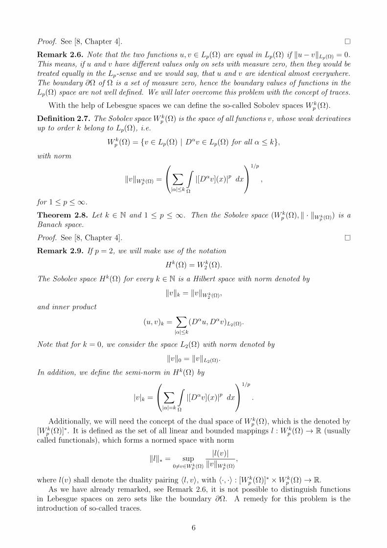
With the help of Lebesgue spaces we can define the so-called Sobolev spaces W kp (Ω).

Definition 2.7. The Sobolev spaceW kp (Ω) is the space of all functions v, whose weak derivatives

up to order k belong to Lp(Ω), i.e.

W kp (Ω) = v ∈ Lp(Ω) | Dαv ∈ Lp(Ω) for all α ≤ k,

with norm

∥v∥Wkp (Ω) =

⎛⎝∑|α|≤k

∫Ω

|[Dαv](x)|p dx

⎞⎠1/p

,

for 1 ≤ p ≤ ∞.

Theorem 2.8. Let k ∈ N and 1 ≤ p ≤ ∞. Then the Sobolev space (W kp (Ω), ∥ · ∥Wk

p (Ω)) is aBanach space.

Proof. See [8, Chapter 4].

Remark 2.9. If p = 2, we will make use of the notation

Hk(Ω) = W k2 (Ω).

The Sobolev space Hk(Ω) for every k ∈ N is a Hilbert space with norm denoted by

∥v∥k = ∥v∥Wk2 (Ω),

and inner product

(u, v)k =∑|α|≤k

(Dαu,Dαv)L2(Ω).

Note that for k = 0, we consider the space L2(Ω) with norm denoted by

∥v∥0 = ∥v∥L2(Ω).

In addition, we define the semi-norm in Hk(Ω) by

|v|k =

⎛⎝∑|α|=k

∫Ω

|[Dαv](x)|p dx

⎞⎠1/p

.

Additionally, we will need the concept of the dual space of W kp (Ω), which is the denoted by

[W kp (Ω)]

∗. It is defined as the set of all linear and bounded mappings l : W kp (Ω) → R (usually

called functionals), which forms a normed space with norm

∥l∥∗ = sup0=v∈Wk

p (Ω)

|l(v)|∥v∥Wk

p (Ω)

,

where l(v) shall denote the duality pairing ⟨l, v⟩, with ⟨·, ·⟩ : [W kp (Ω)]

∗ ×W kp (Ω) → R.

As we have already remarked, see Remark 2.6, it is not possible to distinguish functionsin Lebesgue spaces on zero sets like the boundary ∂Ω. A remedy for this problem is theintroduction of so-called traces.

6

Theorem 2.10 (Trace theorem). Let Ω be a bounded domain with Lipschitz boundary Γ = ∂Ω.Then there exists a bounded linear operator

T : W 1p (Ω) → Lp(Γ)

and a constant c > 0 not depended on u, such that

i) Tu = u|Γ for u ∈ W 1p (Ω) ∩ C(Ω), and

ii)

∥Tu∥Lp(Γ) ≤ c∥u∥W 1p (Ω),

for all u ∈ W 1p (Ω).

Proof. See [12, Chapter 5].

The operator T is called trace operator and Tu is the trace of u ∈ W 1p (Ω) on Γ = ∂Ω. The

image of this mapping defines as new function space on the boundary Γ. For our purpose, it isenough to consider the case p = 2,

T (H1(Ω)) = H1/2(Γ) ⊂ L2(Γ). (2.2)

Thus, we can define H1/2(Γ) as the following space

H1/2(Γ) = w ∈ L2(Γ) | ∃v ∈ H1(Ω) : w = Tv.

The norm in H1/2(Γ) is defined by

∥w∥H1/2(Γ) = inf∥v∥1 | v ∈ H1(Ω), w = Tv.

The dual space of H1/2(Γ) is given by H−1/2(Γ) and its norm is

∥g∥H−1/2(Γ) = supw∈H1/2(Γ)

|g(w)|∥w∥H1/2(Γ)

.

A very important space for our framework is H1(Ω), whose elements have zero trace on theboundary. We denote this space by

H10 (Ω) = v ∈ H1(Ω) | Tv = v|Γ = 0 on Γ = ∂Ω.

Remark 2.11. For the special case p = 2 and zero trace zero trace on the boundary, i.e.W k

2,0(Ω) = Hk0 (Ω), the dual space is denoted by H−k(Ω).

2.3 Important theorems

We close this chapter with important theorems, which we frequently use throughout this work.Considering the fundamental theorem of calculus, we can state the Gauss theorem.

Theorem 2.12 (Gauss theorem). Let Ω ⊂ Rd be a bounded Lipschitz domain and let v : Ω → Rbe a scalar field, φ : Ω → Rd a vector field and σ : Ω → Rd×d a tensor field, all of themsufficiently smooth. Then we have the following identities:∫

∂Ω

v(x)n(x) ds =

∫Ω

∇v(x) dx, (2.3)

∫∂Ω

φ(x) · n(x) ds =∫Ω

div φ(x) dx, (2.4)

∫∂Ω

σ(x) · n(x) ds =∫Ω

div σ(x) dx, (2.5)

where n(x) is the unit outer normal on the boundary ∂Ω.

7

Immediately, we can deduce the following integration by parts formula from Theorem 2.12.

Corollary 2.13. Under the assumptions of Theorem 2.12 the subsequent identities are valid:∫Ω

v(x) div φ(x) dx = −∫Ω

∇v(x) · φ(x) dx+∫∂Ω

v(x)(φ(x) · n(x)) ds, (2.6)

∫Ω

φ(x) div σ(x) dx = −∫Ω

∇φ(x) : σ(x) dx+∫∂Ω

φ(x)(σ(x) · n(x)) ds. (2.7)

Lastly, an important theorem is Banach’s fixed point theorem, which will be used in thesequel to prove existence results of a solution for variational inequalities.

Theorem 2.14 (Banach’s fixed point theorem). Let K be a nonempty closed set in a Banachspace V and let B : K → K be a contraction, i.e. a mapping such that

∥B(u)−B(v)∥V ≤ α∥u− v∥V for all u, v ∈ K,

with a constant α ∈ [0, 1). Then there exists a unique u ∈ K, such that

B(u) = u,

called the fixed point of B. In addition, for any u0 ∈ K, the sequence unn≥0 ⊂ K, defined byB(un) = un+1, converges to the fixed point u, i.e.

∥un − u∥V → 0 as n→ ∞.

Moreover, the following bounds are valid:

∥un − u∥V ≤ α∥un−1 − u∥V ≤ · · · ≤ αn∥u0 − u∥V ,

∥un − u∥V ≤ αn

1− α∥u0 − u1∥V .

Proof. See [1, Chapter 5].

8

Chapter 3

Linear Elasticity

The aim of this chapter is to derive the well known model of linear elasticity and to associatethe equations of the model with their physical meaning. For our purpose, we consider solidelastic materials, which have the essential characteristic that on every part of the body the samephysical properties can be obtained. Usually, external forces are applied to the surface of thematerial, which lead to a deformation of the material body. In the framework of elasticity, thebody returns to its original shape if the external loads are removed, otherwise we fall into thetheory of plasticity. We call the original state of the body the reference configuration and denoteit by Ω0 ⊂ Rd, d = 1, 2, 3, throughout this chapter. Applying forces to the surface (boundary) ofthe material, the body changes its shape to Ωt ⊂ Rd after some time t ∈ R+, which is called thedeformed configuration. Indeed, a broad range of problems for solids are described by linearelasticity realistically. We only consider macroscopic, i.e. large scale, behavior of materialsfor the elasticity problem since it is appropriate for almost all engineering purposes and weignore the microscopic, or small scale, behavior. The goal is now to derive the mathematicalmodel describing the displacement of a so-called elastic St.Venant-Kirchhoff material after thedeformation based on the work of [2, Chapter 3], [3, Chapter 9], [4, Chapter 6], [7, Chapter4], [40] and [49]. The equations of the model will be derived from general physical principlessuch as conservation laws, on one hand and from constitutive laws, which describe the materialproperties, on the other hand.

3.1 Eulerian and Lagrangian coordinates and

deformation

In general, it is important to differentiate between the material points of the body in thereference configuration and the deformed configuration. For this purpose, we define the Eulerianand Lagrangian coordinates, respectively.

Definition 3.1. The Lagrangian coordinates describe the position of the material points in thereference configuration (at time t = 0), which is given by

X =d∑i=1

Xiei, (3.1)

where Xi are the coefficients of the position vector in the reference configuration and ei are theunit vectors of Rd.

Definition 3.2. The spatial or Eulerian coordinates describe the position of the material points

9

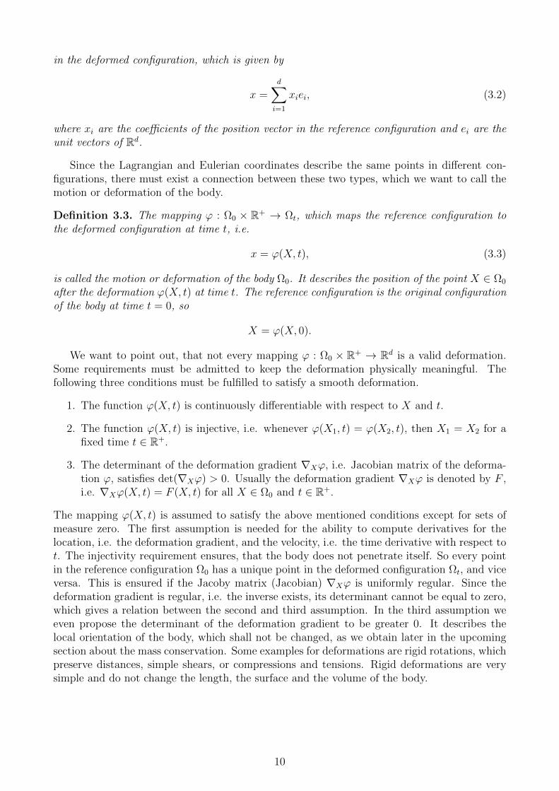
in the deformed configuration, which is given by

x =d∑i=1

xiei, (3.2)

where xi are the coefficients of the position vector in the reference configuration and ei are theunit vectors of Rd.

Since the Lagrangian and Eulerian coordinates describe the same points in different con-figurations, there must exist a connection between these two types, which we want to call themotion or deformation of the body.

Definition 3.3. The mapping φ : Ω0 × R+ → Ωt, which maps the reference configuration tothe deformed configuration at time t, i.e.

x = φ(X, t), (3.3)

is called the motion or deformation of the body Ω0. It describes the position of the point X ∈ Ω0

after the deformation φ(X, t) at time t. The reference configuration is the original configurationof the body at time t = 0, so

X = φ(X, 0).

We want to point out, that not every mapping φ : Ω0 × R+ → Rd is a valid deformation.Some requirements must be admitted to keep the deformation physically meaningful. Thefollowing three conditions must be fulfilled to satisfy a smooth deformation.

1. The function φ(X, t) is continuously differentiable with respect to X and t.

2. The function φ(X, t) is injective, i.e. whenever φ(X1, t) = φ(X2, t), then X1 = X2 for afixed time t ∈ R+.

3. The determinant of the deformation gradient ∇Xφ, i.e. Jacobian matrix of the deforma-tion φ, satisfies det(∇Xφ) > 0. Usually the deformation gradient ∇Xφ is denoted by F ,i.e. ∇Xφ(X, t) = F (X, t) for all X ∈ Ω0 and t ∈ R+.

The mapping φ(X, t) is assumed to satisfy the above mentioned conditions except for sets ofmeasure zero. The first assumption is needed for the ability to compute derivatives for thelocation, i.e. the deformation gradient, and the velocity, i.e. the time derivative with respect tot. The injectivity requirement ensures, that the body does not penetrate itself. So every pointin the reference configuration Ω0 has a unique point in the deformed configuration Ωt, and viceversa. This is ensured if the Jacoby matrix (Jacobian) ∇Xφ is uniformly regular. Since thedeformation gradient is regular, i.e. the inverse exists, its determinant cannot be equal to zero,which gives a relation between the second and third assumption. In the third assumption weeven propose the determinant of the deformation gradient to be greater 0. It describes thelocal orientation of the body, which shall not be changed, as we obtain later in the upcomingsection about the mass conservation. Some examples for deformations are rigid rotations, whichpreserve distances, simple shears, or compressions and tensions. Rigid deformations are verysimple and do not change the length, the surface and the volume of the body.

10

Ω0

Ω1

Ω2

Ω3

X

x = ϕ(X,2)

ϕ(∙,3)

ϕ(∙,2)

ϕ(∙,1)

u(X,2) = ϕ(X,2) - X

Figure 3.1: Deformation of body Ω0 at time t = 1, 2, 3 and the displacement u of a point X.

3.2 Displacement, velocity and acceleration

Next, we describe the displacement, which plays an important role in the equations of themathematical model of elasticity. Shortly, we give the definitions of the velocity and theacceleration, but we recommend [21, Chapter 2] for detailed description and their physicalproperties. We want to start with the definition of the displacement.

Definition 3.4. The displacement u ∈ Rd of a material point X ∈ Ω0 is the difference betweenthe current position x ∈ Ωt and the original position of the point X and is defined by

u(X, t) = x−X = φ(X, t)−X = φ(X, t)− φ(X, 0). (3.4)

Figure 3.1 illustrates the deformation of a body Ω0 and the displacement of a point X. Thevelocity and the acceleration in the Lagrangian coordinates are the following.

Definition 3.5. The velocity V : Ω0 × R+ → Rd in Lagrangian coordinates is defined by

V (X, t) =∂

∂tφ(X, t) =

∂

∂tu(X, t), (3.5)

which is the rate of change of the position for a fixed material point X ∈ Ω.The acceleration A : Ω0 × R+ → Rd in Lagrangian coordinates is defined by

A(X, t) =∂

∂tv(X, t) =

∂2

∂t2u(X, t), (3.6)

which is the rate of change of the velocity for a fixed material point X ∈ Ω.

It is possible to obtain the velocity and the acceleration in terms of the spatial coordinates.For this reason we will make use of the chain rule.

11

Definition 3.6. The velocity v : Ωt × R+ → Rd in spatial coordinates is defined by

v(x, t) = V (φ−1(x, t), t). (3.7)

The acceleration a : Ωt × R+ → Rd in spatial coordinates is given by

a(x, t) = A(φ−1(x, t), t). (3.8)

Remark 3.7. Note that the time derivatives are usually called material derivatives. Further-more, the following relation in spatial coordinates holds.

a(x, t) =D

Dtv(x, t) =

D

Dtv(φ(X, t), t) =

∂

∂tv(x, t) + v · ∇Xv, (3.9)

where the last term is called the transport term and is defined by v · ∇Xv =d∑i=1

vi∂v(x,t)∂xi

. The

last equality in (3.9) follows from the chain rule.

3.3 Strain tensor

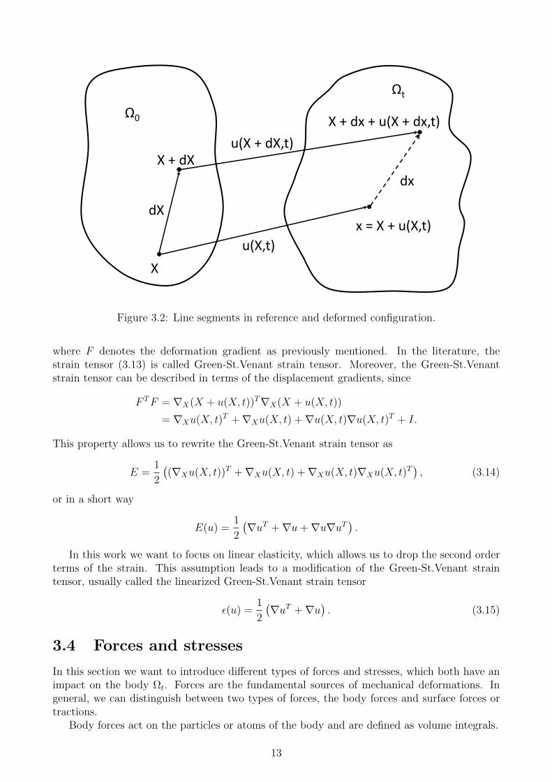
A very important quantity in Continuum mechanics is the so-called strain measure. It is themeasure of deformation representing the displacement between two particles in the deformedbody relative to a reference length in the reference configuration. Figure 3.2 illustrates thisincident, where the reference length is denoted by dX in the reference configuration and therelative length in deformed configuration is denoted by dx. The mostly common strain measurein connection with Continuum mechanics is the so-called Green strain E.

Definition 3.8. The Green strain tensor E is defined by

dx2 − dX2 = 2 dX · E · dX, (3.10)

where dx2 is the squared length of a line segment after the deformation with original squaredlength dX2.

The tensor E measures the strain in an element dX as the original coordinates of a pointX are moved to new coordinates x by

x = X + u. (3.11)

Considering the line segments in the infinitesimal case and differentiating (3.11) gives

dx =∂x

∂XdX = ∇Xφ dX =

∂(X + u)

∂XdX. (3.12)

Substitution of (3.12) into the definition of the Green strain tensor (3.10) gives

dX · (∇Xφ(X, t)T∇Xφ(X, t)− I − 2E) · dX = 0,

which can be rewritten as

E =1

2(∇Xφ(X, t)

T∇Xφ(X, t)− I) =1

2(F TF − I), (3.13)

12

Ω0

Ωt

X

X + dX

dX

X + dx + u(X + dx,t)

u(X + dX,t)

u(X,t)

x = X + u(X,t)

dx

Figure 3.2: Line segments in reference and deformed configuration.

where F denotes the deformation gradient as previously mentioned. In the literature, thestrain tensor (3.13) is called Green-St.Venant strain tensor. Moreover, the Green-St.Venantstrain tensor can be described in terms of the displacement gradients, since

F TF = ∇X(X + u(X, t))T∇X(X + u(X, t))

= ∇Xu(X, t)T +∇Xu(X, t) +∇u(X, t)∇u(X, t)T + I.

This property allows us to rewrite the Green-St.Venant strain tensor as

E =1

2

((∇Xu(X, t))

T +∇Xu(X, t) +∇Xu(X, t)∇Xu(X, t)T), (3.14)

or in a short way

E(u) =1

2

(∇uT +∇u+∇u∇uT

).

In this work we want to focus on linear elasticity, which allows us to drop the second orderterms of the strain. This assumption leads to a modification of the Green-St.Venant straintensor, usually called the linearized Green-St.Venant strain tensor

ϵ(u) =1

2

(∇uT +∇u

). (3.15)

3.4 Forces and stresses

In this section we want to introduce different types of forces and stresses, which both have animpact on the body Ωt. Forces are the fundamental sources of mechanical deformations. Ingeneral, we can distinguish between two types of forces, the body forces and surface forces ortractions.

Body forces act on the particles or atoms of the body and are defined as volume integrals.

13

Definition 3.9. The body forces Fb ∈ Rd acting on a part of a body B ⊂ Ωt are defined as

Fb(B) =

∫B

f(x, t) dx, (3.16)

where f : Ωt × R+ → Rd is called the body force density.

The counterpart of body forces are surface forces, which act only on the surface of the bodyor parts of it. These forces depend not only on the points on the surface, i.e. location, but alsoon the normal vector of the points on the surface.

Definition 3.10. Let Σ = y ∈ Rd | ∥y∥ = 1 be the set of all directions. The surface forcesFc ∈ Rd acting on a part of a body B ⊂ Ωt are defined as

Fc(B) =

∫∂B

t(x, t, n(x)) ds, (3.17)

where t : Ωt×R+×Σ → Rd is called the surface force density and n(x) ∈ Σ is the unit outwardnormal vector at x ∈ ∂B.

The total forces Fg ∈ Rd acting on a part of a body B ⊂ Ωt are the sum of the body forcesand surface forces,

Fg(B) = Fb(B) + Fc(B). (3.18)

The stress is a measure for the force on a surface of a body or parts of it on which externalforces (body or surface forces) are applied. In this work we introduce the Cauchy stress σ. Theexistence of the Cauchy stress is the result of Cauchy’s Theorem.

Theorem 3.11 (Cauchy’s Theorem). Let t be as in Definition 3.10 and continuously differ-entiable in every component and variable. Then there exists a tensor field σ, continuouslydifferentiable in every component and variable, called the Cauchy tensor, such that

σ(x, t)T · n(x) = t(x, t, n(x)) for all x ∈ Ωt, t ∈ R+ and n ∈ Σ. (3.19)

Remark 3.12. We will see that the Cauchy stress tensor is symmetric which follows from theconservation of angular momentum in the next section. In the literature, another stress measurecan be found which we refer to as the (second) Piola-Kirchhoff stress tensor. It is defined interms of the Cauchy stress tensor by

ΣT2 (X, t) = det(F (X, t))F−1(X, t) σ(φ(X, t)) F−T (X, t) for all X ∈ Ω0,

where F = ∇Xφ(X, t). By this representation the symmetry of the Piola-Kirchhoff stress tensorfollows inherently from the symmetry of the Cauchy stress tensor. For detailed description ofthese two stress measures we give [2, Chapter 3] as a reference.

Due to the symmetry of Cauchy stress tensor σ, (3.19) can be rewritten as

σ · n = t. (3.20)

For the remainder of this work we will only consider the Cauchy stress tensor σ.

14

3.5 Conservation laws

The purpose of this section is to present the conservation laws, which give a part of the fun-damental equations of continuum mechanics. These laws must be always satisfied in physicalsystems. The relevant laws are the conservation of mass, conservation of linear momentumand conservation for angular momentum. For a detailed description of the conservation lawswe refer to [2, Chapter 3], [4, Chapter 6] and [40]. In order to derive these laws, fundamentaltheorems are needed. The first one is the already introduces Gauss Theorem 2.12. Anotherfundamental theorem is Reynolds Transport Theorem. It describes the rate of change for amaterial domain.

Theorem 3.13 (Reynolds Transport Theorem). Let f : Ωt ×R+ → Rd be a piece-wise contin-uously differentiable function. Then the following relation holds:

D

Dt

∫Ωt

f(x, t) dx =

∫Ωt

∂f(x, t)

∂t+ div (v(x, t)f(x, t)) dx, (3.21)

where v is the velocity of the body.

Proof. See [10, Chapter 5].

With the help of these two fundamental theorems we can derive the mathematical equationsfor the conservation laws of interest. We want to start with the mass conservation.

3.5.1 Conservation of mass

The mass m(B) for any part B of continuum mechanical body Ωt is given by

m(B) =

∫B

ρ(x, t) dx, (3.22)

where ρ : Ωt × R+ → R+ is the mass density of the body. The conservation of mass demandsthat the mass of any part of the body is constant, i.e. the mass does not change, since no masscan be added or removed from the boundary. Mathematically, the conservation of mass can bedescribed as

Dm

Dt=

D

Dt

∫B

ρ(x, t) dx = 0. (3.23)

Using Reynolds Transport Theorem 3.13, we deduce from (3.23) that∫B

(∂ρ(x, t)

∂t+ div (ρ(x, t)v(x, t))

)dx = 0. (3.24)

Since the mass conservation holds for any part B of the body Ωt, it follows from (3.24) that

∂ρ(x, t)

∂t+ div (ρ(x, t)v(x, t)) = 0 in Ωt. (3.25)

Equation (3.25) is the mass conservation equation, also called continuity equation.

15

3.5.2 Conservation of linear momentum

In this subsection we derive the equations of linear momentum, also known as momentumconservation principle or balance of momentum. The linear momentum p : Ωt × R+ → Rd

characterizes the status of motion of a body and is defined as the product of the mass andvelocity of the body Ωt, i.e.

p(x, t) =

∫Ωt

ρ(x, t)v(x, t) dx, (3.26)

where ρ is the density of Ωt, v the velocity and ρv is the linear momentum per unit volume.The conservation of linear momentum states, that the material time derivative of the linear

momentum is equal to the total force (3.18), which can be written as

D

Dtp(x, t) = Fg(Ωt),

or equivalently

D

Dt

∫Ωt

ρ(x, t)v(x, t) dx =

∫Ωt

f(x, t) dx+

∫∂Ωt

t(x, t, n(x)) ds. (3.27)

Using now Reynolds Transport Theorem 3.13 for the material derivative in (3.27), we get that

D

Dt

∫Ωt

ρv dx =

∫Ωt

∂(ρv)

∂t+ div

(v(ρv)T

)dx

=

∫Ωt

ρ∂v

∂t+ v

∂ρ

∂t+ div

(v(ρv)T

)dx,

(3.28)

where the product rule has been used in the last step. Furthermore, we can use the obviousproperty that, div

(v(ρv)T

)= (∇v)(ρv)T + v div (ρv) to obtain∫

Ωt

ρ∂v

∂t+ v

∂ρ

∂t+ div

(v(ρv)T

)dx

=

∫Ωt

ρ∂v

∂t+ v

∂ρ

∂t+ (∇v)(ρv)T + v div (ρv) dx,

such that (3.28) reduces due to the mass conservation (3.25) to

D

Dt

∫Ωt

ρv dx =

∫Ωt

ρ∂v

∂t+ (∇v)(ρv)T dx. (3.29)

With the help of (3.29) we can rewrite (3.27) as∫Ωt

ρ∂v

∂t+ (∇v)(ρv)T dx =

∫Ωt

f dx+

∫∂Ωt

t ds. (3.30)

Considering now Cauchy’s Theorem 3.11 and the Gauss Theorem 2.12 for the boundary ex-pression, we deduce from (3.30) the conservation of linear momentum in the integral form∫

Ωt

ρ∂v

∂t+ (∇v)(ρv)T dx =

∫Ωt

f dx+

∫Ωt

div σ dx,

16

which is equivalent to ∫Ωt

(ρ∂v

∂t+ (∇v)(ρv)T − f − div σ

)dx = 0,

and therefore we get the equation of the conservation of linear momentum

ρD

Dtv = ρ

(∂v

∂t+ (∇v)v

)= f + div σ. (3.31)

Remark 3.14. In fact, the conservation of linear momentum is equivalent to Newton’s secondlaw, which states that the product of mass and acceleration equals the force of a body.

3.5.3 Equilibrium equation

The equilibrium equation is a consequence of the conservation of linear momentum equation(3.31), since in many problems the loads are applied slowly and hence, the acceleration can beneglected. The equilibrium equation reads as

f + div σ = 0 or − div σ = f. (3.32)

3.5.4 Conservation of angular momentum

The angular momentum can be obtained by taking the cross product of each term in (3.27)with the position vector x. Its integral from is therefore

D

Dt

∫Ωt

x× ρv dx =

∫Ωt

x× f dx+

∫∂Ωt

x× t ds. (3.33)

As it is mentioned before, the conservation of angular momentum yields the symmetry of thestress tensor. We want to state this property as a theorem.

Theorem 3.15. Let ρ, v, f and t be sufficiently smooth and let the conservation of linearmomentum (3.31) and the conservation of angular momentum (3.33) hold. Then the stresstensor σ is symmetric.

Proof. [10, Chapter 5].

3.6 Constitutive laws

The section before has given a quick overview about the physical laws that any material mustsatisfy in continuum mechanics. In this section we want to specify the material properties,which are described by so-called constitutive or material laws. The constitutive equationscharacterize the material and give a relation between the stress and the deformation historyof the body in terms of the so-called response function. We briefly give the material equationfor an elastic, St.Venant-Kirchhoff material. For a more detailed description we refer to [2,Chapter 5], [10, Chapter 5] and [40].

We start with the definition of an elastic body.

17

Definition 3.16 (Elastic material). A material is said to be elastic if the stress σ dependson the material point and the deformation gradient, i.e. there exists a function T , called theresponse function, such that

σ(x, t) = T (X,∇Xφ(X, t)). (3.34)

The elastic material is called homogeneous if the stress only depends on the deformation gradientand not on the reference points, i.e. σ = T (∇Xφ(X, t)). Otherwise, the material is said to beheterogeneous.

Not every response function of an elastic material describes a real physical body. In order tohandle this incidence we require that the constitutive equation shall not depend on the choiceof coordinate system. This kind of requirement is also known as the material frame indifferenceor objectivity. We always assume that the response function fulfills this requirement and referto [2, Chapter 3] for the complete description.

Finally, we need a relation between the stress and the strain, which falls into the frameworkof the constitutive laws. A linear strain-stress relation is the so-called Hooke’s law.

Definition 3.17 (Hooke’s law). The stress-strain relation of an elastic material can be describedby Hooke’s law, which is

σ = CE(u) or σij(u) =d∑

k,l=1

CijklEkl(u) for i, j = 1, ..., d. (3.35)

where C = (Cijkl)di,j,k,l=1 ∈ Rd×d×d×d is a tensor of forth order with the symmetry property

Cijkl = Cjikl = Cklij.

Remark 3.18. Note, that Hooke’s law for the linearized strain tensor reads as

σ = Cϵ(u) or σij(u) =d∑

k,l=1

Cijklϵkl(u) for i, j = 1, ..., d. (3.36)

Summarizing all the conservation laws and taking the constitutive laws into account we arenow able to give the mathematical model for the deformation of an elastic St.Venant-Kirchhoffmaterial. We assume that the body is clamped on a certain part of the surface ΓD and we onlyapply the tractions on the rest of the surface ΓF , i.e. |ΓD| > 0, ΓD∪ΓF = ∂Ω and ΓD∩ΓF = ∅.The problem is: Find the displacement u, such that

−div σ(u) = f in Ω, (3.37a)

u = 0 on ΓD, (3.37b)

σ(u) · n = t on ΓF , (3.37c)

σ(u) = Cϵ(u), (3.37d)

ϵ(u) =1

2

(∇u+ (∇u)T

). (3.37e)

Remark 3.19. Hooke’s law for an isotropic material under consideration of the frame indif-ference and the Rivlin-Ericksen Theorem (cf. [27]) can be written as

σ(u) = 2µϵ(u) + λtr(ϵ(u))I,

where µ and λ are called the Lame parameters. The Lame coefficients can be also described interms of Young’s Modulus E and Poisson’s ration ν by

µ =E

2(1 + ν), λ =

Eν

(1 + ν)(1− 2ν). (3.38)

18

Chapter 4

Signorini and Obstacle Problem

The aim of this chapter is to formulate the classical Signorini problem and give the mathemat-ical model with its corresponding physical background. The Signorini problem is the basis forcontact problems in solid mechanics and describes the contact of a linearly elastic body with africtionless rigid foundation. We kick of this chapter with the introduction of the contact con-ditions and the raising of classical mathematical PDE model following the ideas of [16, Chapter2], [18, Chapter 2] and [42, Chapter 2]. The variational formulation of this problem leads toa variational inequality, whose analysis will be the topic of the next chapter. The end of thischapter addresses a simplified version of the Signorini problem, also called simplified Signoriniproblem, and a special obstacle problem. Just as the classical Signorini problem, each of theseproblems involves the contact between a linearly elastic body and a rigid foundation. We referto [13, Chapter 2], [14, Chapter 4], [28, Chapter 1] and [39] for their detailed description.

We assume small deformations throughout this chapter, such that the previously describedlinear elasticity theory will be a part of the model for contact problems. In fact, the rigidfoundation plays the role of a constraint on the boundary of the body, which can be seen inthe upcoming section.

4.1 Classical Signorini problem

The Signorini problem investigates the deformation of an elastic body when it comes into con-tact with a rigid foundation. The contact boundary depends on the displacement of the elasticbody, which makes it to an unknown variable in the model. Due to fact that the contact sur-face is a-priori unknown, the Signorini problem is highly nonlinear and non-differentiable withrespect to the displacement. We start this section with the description of the contact condi-tions, where the focus lies on the linearized contact. With the help of the contact conditions,we can formulate the classical model of the Signorini problem and conclude this section withits variational form. We will see that the variational form leads to variational inequalities byreason of the contact conditions. The contribution of this section is based on [16, Chapter 2],[18, Chapter 2] and [42, Chapter 2].

As we have introduced in the chapter before, we describe the particles of the body Ω0 ⊂ R3 inreference configuration by Lagrangian coordinates X = (X1, X2, X3). The body is set in motionand changes its location and shape in every time step t, where the position x = (x1, x2, x3)of the particles of the deformed body Ωt ⊂ R3 can be described by the deformation φ, i.e.x = φ(X, t). The deformation φ satisfies the conditions in Definition 3.3 as well as the belowrequirements for a smooth deformation. The displacement of a point X ∈ Ω0 is given as in(3.4), i.e. u(X, t) = φ(X, t)−X.

From now on, we consider the deformation of the body only for one time step or ratherfor a fixed time t1. This consideration allows us to ignore the dependence on the time t.

19

Consequently, the reference configuration will be denoted by Ω and the deformation by φ(X).The displacement u is then given as

u(X) = φ(X)−X. (4.1)

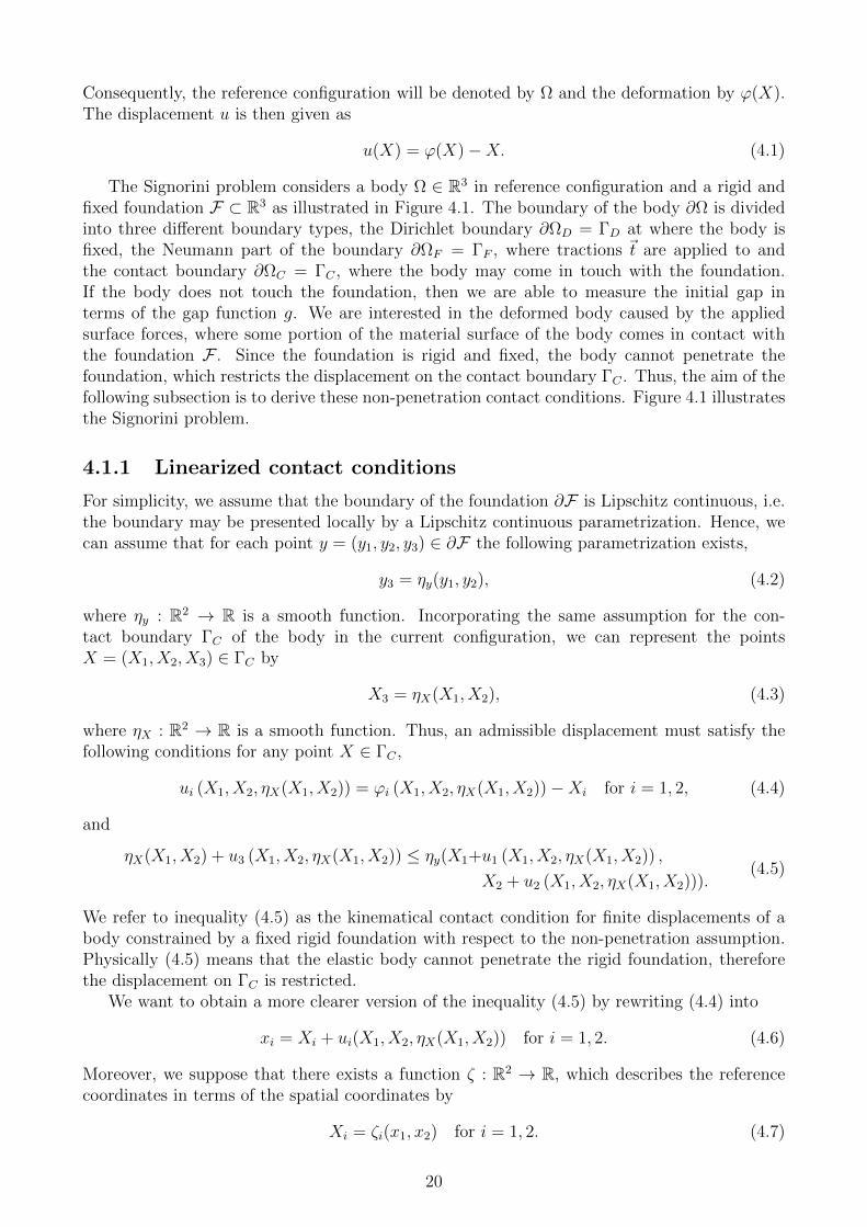
The Signorini problem considers a body Ω ∈ R3 in reference configuration and a rigid andfixed foundation F ⊂ R3 as illustrated in Figure 4.1. The boundary of the body ∂Ω is dividedinto three different boundary types, the Dirichlet boundary ∂ΩD = ΓD at where the body isfixed, the Neumann part of the boundary ∂ΩF = ΓF , where tractions t are applied to andthe contact boundary ∂ΩC = ΓC , where the body may come in touch with the foundation.If the body does not touch the foundation, then we are able to measure the initial gap interms of the gap function g. We are interested in the deformed body caused by the appliedsurface forces, where some portion of the material surface of the body comes in contact withthe foundation F . Since the foundation is rigid and fixed, the body cannot penetrate thefoundation, which restricts the displacement on the contact boundary ΓC . Thus, the aim of thefollowing subsection is to derive these non-penetration contact conditions. Figure 4.1 illustratesthe Signorini problem.

4.1.1 Linearized contact conditions

For simplicity, we assume that the boundary of the foundation ∂F is Lipschitz continuous, i.e.the boundary may be presented locally by a Lipschitz continuous parametrization. Hence, wecan assume that for each point y = (y1, y2, y3) ∈ ∂F the following parametrization exists,

y3 = ηy(y1, y2), (4.2)

where ηy : R2 → R is a smooth function. Incorporating the same assumption for the con-tact boundary ΓC of the body in the current configuration, we can represent the pointsX = (X1, X2, X3) ∈ ΓC by

X3 = ηX(X1, X2), (4.3)

where ηX : R2 → R is a smooth function. Thus, an admissible displacement must satisfy thefollowing conditions for any point X ∈ ΓC ,

ui (X1, X2, ηX(X1, X2)) = φi (X1, X2, ηX(X1, X2))−Xi for i = 1, 2, (4.4)

and

ηX(X1, X2) + u3 (X1, X2, ηX(X1, X2)) ≤ ηy(X1+u1 (X1, X2, ηX(X1, X2)) ,

X2 + u2 (X1, X2, ηX(X1, X2))).(4.5)

We refer to inequality (4.5) as the kinematical contact condition for finite displacements of abody constrained by a fixed rigid foundation with respect to the non-penetration assumption.Physically (4.5) means that the elastic body cannot penetrate the rigid foundation, thereforethe displacement on ΓC is restricted.

We want to obtain a more clearer version of the inequality (4.5) by rewriting (4.4) into

xi = Xi + ui(X1, X2, ηX(X1, X2)) for i = 1, 2. (4.6)

Moreover, we suppose that there exists a function ζ : R2 → R, which describes the referencecoordinates in terms of the spatial coordinates by

Xi = ζi(x1, x2) for i = 1, 2. (4.7)

20

Rigid Foundation ℱ

g

ΓD

Ω

ΓC

ΓF

Ԧ𝑡

Figure 4.1: Contact between the body Ω and a rigid foundation F .

Then the kinematical contact condition (4.5) can be rewritten as

ηX(x1, x2) + u3(x1, x2) ≤ ηy(x1, x2), (4.8)

where

ηX(x1, x2) = ηX (ζ1(x1, x2), ζ2(x1, x2)) ,

u3(x1, x2) = u3 (ζ1(x1, x2), ζ2(x1, x2), ηX(ζ1(x1, x2), ζ2(x1, x2))) ,

ηy(x1, x2) = ηy(X1 + u1, X2 + u2).

Condition (4.8) is derived just as (4.5) from kinematical observations. However, it also mustbe compatible with the stress condition on the contact surface ΓC . We emphasize at this point,that no external tractions are applied on ΓC . Nevertheless stress is developed if the elasticbody touches the rigid foundation. For this purpose, let σ = σ(x1, x2, x3) be the Cauchy stresstensor of particle X ∈ Ω whose position is x = (x1, x2, x3) and let n = (n1, n2, n3) be the unitouter normal of ΓC . The normal and tangential components of the stress vector σ · n at theboundary of the body ∂Ω = Γ are (σ ·n)n and (σ ·n)T as illustrated in Figure 4.2, respectively,where

(σ · n)n = ((σ · n) · n)n,(σ · n)T = σ · n− (σ · n)n.

(4.9)

Usually, the quantities

σn(x) = σij(x)ni(x)nj(x),

σTi(x) = σij(x)nj(x)− σn(x)ni(x),1 ≤ i, j ≤ 3, (4.10)

are used in the literature, where x = φ−1(X) ∈ ΓC and σn denotes the length of (σ · n)n. Inthe sequel we will call σn the normal component of the stress and σTi the i− th coordinate oftangential component of the stress.

21

𝜎 ∙ 𝑛

𝑥 ∈ Γ𝐶 𝜎𝑇

𝜎𝑛𝑛

Figure 4.2: Normal and tangential component of stress σ · n at point x ∈ ΓC .

We can make physical observations analyzing these components of the stress tensor. Firstly,if there is no contact between the body and the foundation, then there is no stress at all,therefore σn = 0. On the other hand, if the body is in touch with the foundation on ΓC , thennormal stress σn must be developed on ΓC . Secondly, the tangential stress σTi must be zero onΓC , since the foundation surface ∂F is frictionless. The mathematical interpretation of thesephysical observations is

σn(x) = 0 if ηX(x1, x2) + u3(x1, x2) < ηy(x1, x2),

σn(x) ≤ 0 if ηX(x1, x2) + u3(x1, x2) = ηy(x1, x2),

σTi(x) = 0,

(4.11)

for 1 ≤ i ≤ 3 and for all x = φ−1(X) ∈ ΓC . Considering condition (4.8) and the first twoconditions in (4.11), it results the following relation for the normal vector,

σn(x) (ηX(x1, x2) + u3(x1, x2)− ηy(x1, x2)) = 0, (4.12)

for all x ∈ ΓC . Gathering all the considerations for the contact between the body and the rigidfoundation, we deduce the general contact conditions in the frictionless case

ηX(x1, x2) + u3(x1, x2) ≤ ηy(x1, x2),

σn(x) ≤ 0,

σTi(x) = 0,

σn(x) (ηX(x1, x2) + u3(x1, x2)− ηy(x1, x2)) = 0,

(4.13)

for all x ∈ ΓC and 1 ≤ i ≤ 3.The goal is now to derive the linearized contact conditions from (4.13) in terms of the refer-

ence configuration Ω. For this reason, we assume that the body makes ”small” displacements

22

relative to its initial position. Consequently, the distance between the body and the rigid foun-dation is rather short, which allows us to consider them to be essentially parallel in the sensethat the unit normal vector n and the normalized gap function g can be obtained in terms ofthe body surface ΓC . In addition, we assume that the parametrizations ηX and ηy have at leastcontinuous first partial derivatives and bounded second partial derivatives everywhere in theirrespective domains. Then we receive that

xi = Xi + ui(X1, X2, X3) = Xi + ui(X1, X2, ηX(X1, X2))

= Xi + ui(x1 +X1 − x1, x2 +X2 − x2, ηX(x1, x2) + ηX(X1, X2)− ηX(x1, x2))

= Xi + ui(x1 − u1, x2 − u2, ηX(x1, x2)− u3).

(4.14)

Making use of the Taylor expansion (c.f. [23, Chapter 4]) yields

xi = Xi + ui(x1, x2, ηX(x1, x2)) +O(|ui|2, |ui,j|2) for i = 1, 2, 3, (4.15)

where O(·) denotes the higher order terms of u and corresponding partial derivatives. Sincewe want to linearize condition (4.15), we drop the higher order terms and keep the linearexpressions, which lead to

xi = Xi + ui(x1, x2, ηX(x1, x2)), (4.16)

for x ∈ ΓC . Similarly, we conclude that

ηX(X1, X2) = ηX(x1 +X1 − x1, x2 +X2 − x2) = ηX(x1 − u1, x2 − u2). (4.17)

Using again the Taylor expansion and dropping the higher order terms yields

ηX(X1, X2) = ηX(x1, x2)−∂ηX(x1, x2)

∂x1u1 −

∂ηX(x1, x2)

∂x2u2. (4.18)

Likewise, we obtain by retaining the linear terms that

u3(X1, X2, ηX(X1, X2)) = u3(x1, x2, ηX(x1, x2)). (4.19)

We can insert now the linearized conditions (4.16), (4.18) and (4.19) into the kinematicalcontact condition (4.5) to deduce the linearized kinematical contact condition

ηX(x1, x2)−∂ηX(x1, x2)

∂x1u1 −

∂ηX(x1, x2)

∂x2u2 + u3(x1, x2, ηX(x1, x2)) ≤ ηy(x1, x2). (4.20)

Defining now the direction n(x) =(−∂ηX(x1,x2)

∂x1,−∂ηX(x1,x2)

∂x2, 1), we can equivalently rewrite

(4.20) as(−∂ηX(x1, x2)

∂x1,−∂ηX(x1, x2)

∂x2, 1

)· (u1, u2, u3)T ≤ ηy(x1, x2)− ηX(x1, x2), (4.21)

for all x ∈ ΓC . The direction vector n(x) is defined as the outward normal vector for the point

x on the contact boundary ΓC . Dividing (4.21) by ∥n∥ =

√12 +

(∂ηX(x1,x2)

∂x1

)2+(∂ηX(x1,x2)

∂x2

)2we obtain the normalized and linearized contact condition

u(x) · n(x) ≤ g(x) for all x ∈ ΓC , (4.22)

23

where

n(x) =n(x)

∥n(x)∥,

g(x) =ηy(x1, x2)− ηX(x1, x2)

∥n(x)∥.

The function g : R3 → R denotes the normalized initial gap between the surface of the founda-tion ∂F and ΓC . Due to the assumptions of small displacement and the close initial positionsof the surfaces of the body and the rigid foundation, i.e.

ηy − ηX = O(|u3|),u(X) · n(X) = u(x) · n(x) +O(|un,i| · |un|),

g(X) = g(x) +O(|u3| · |u3,i|),

we can write condition (4.22) in terms of particle X ∈ ΓC in the reference configuration withrespect to its outer normal n(X) , which is

un(X)− g(X) ≤ 0, (4.23)

where un(X) = u(X) · n(X). Finally, we can derive from (4.13) the fully linearized contactconditions in the frictionless case,

un(X)− g(X) ≤ 0,

Tn(X) ≤ 0,

TTi(X) = 0,

Tn(X) (un(X)− g(X)) = 0,

(4.24)

for all X ∈ ΓC , where T shall to be understood as the Cauchy stress tensor measured in thereference configuration, i.e. Tn(X) = σn(φ(X)) and TTi(X) = σTi(φ(X)), and Tn and TTi aredefined as in (4.10).

4.1.2 Classical form

With the help of the linearized contact conditions, we are now able to formulate the Signoriniproblem in its classical form by terms of differential equations. For the rest of this chapter, wealways consider the framework of linear elasticity. For this reason we act on the assumption ofthe reference configuration Ω and denote its particles by x ∈ Ω. The Cauchy stress T measuredin the reference configuration as in (4.24) will be denoted as σ, i.e. T = σ. Note that thelinearized contact conditions (4.24) are described with respect to the particles X = x. If wetake Hook’s law (3.36) for the linear strain tensor into account, then the stress can be writtenas σ(x) = σ(x, u) = σ(u). Thus, (4.24) is still valid for the stress tensor σ(u) described in termsof the displacement u.

As already mentioned, we assume the body Ω to be clamped along a part of the boundaryΓD and surface tractions t are applied to a certain part of the body ΓF . The contact surface,where the body may come in touch with the rigid foundation F , is denoted by ΓC . The actualcontact surface is not known in advance but it is assumed to be a subset of ΓC . The initial gap gbetween the body and the rigid foundation is known. Recalling the equilibrium equation (3.32)and taking the boundary conditions into account, we are able formulate the component-wiseclassical frictionless Signorini problem in linear elasticity for elastic and homogeneous materials

24

given by Hooke’s law (3.36): Find the displacement u, such that

− ∂

∂xjσij(u) = fi in Ω, (4.25a)

ui = 0 on ΓD, (4.25b)

σij(u)nj = ti on ΓF , (4.25c)

σTi(u) = 0,

σn(u)(un − g) = 0,

un − g ≤ 0,

σn(u) ≤ 0,

⎫⎪⎪⎪⎬⎪⎪⎪⎭ on ΓC , (4.25d)

σij(u) =3∑

k,l=1

Cijklϵij(u), (4.25e)

ϵij(u) =1

2

(∂ui∂xj

+∂uj∂xi

), (4.25f)

where

σn(u) = σij(u)ninj,

σTi(u) = σij(u)nj − σn(u)ni, for 1 ≤ i, j ≤ 3.

4.1.3 Variational form

In this section, we want to derive the variational form of the classical Signorini problem. Furthis purpose, let V = v ∈ [H1(Ω)]3 | v = 0 on ΓD be the vector-valued Hilbert space, whichdenotes the set of virtual displacements. We assume, that the functions v ∈ V are sufficientlysmooth in the sense that every operation we want to do is well defined. Particularly, this meansthat the virtual work

∫Ωσ(u) : ϵ(u) is well defined for all u, v ∈ V . For any given positive gap

function g : ΓC → R, the contact conditions can be incorporated by the convex subset K ⊂ Vdefined as the set of admissible displacements satisfying the kinematic contact conditions,

K = v ∈ V | vn − g ≤ 0 on ΓC. (4.26)

It turns out that the variational formulation of the Signorini problem is indeed a variationalinequality. It can be formulated as: Find u ∈ K, such that

a(u, v − u) ≥ ⟨F, v − u⟩ for all v ∈ K, (4.27)

where

a(u, v) =

∫Ω

σij(u)∂vi∂xj

dx,

⟨F, v⟩ =∫Ω

fivi dx+

∫ΓF

tivi ds.

The next theorem confirms that a solution of the classical form the Signorini problem can becharacterized by the variational inequality and conversely.

Theorem 4.1. Let u ∈ K be a sufficiently smooth solution of the classical form of the Signoriniproblem (4.25). Then u solves the variational inequality (4.27). On the other hand, if u ∈ Ksolves (4.27) and is sufficiently smooth, then it is also a solution of (4.25).

25

Proof. Firstly, we prove that a solution u ∈ K of (4.25) solves (4.27). For this purpose, letv ∈ K be an arbitrary element. We multiply (4.25a) with the test function v − u ∈ K andintegrate over the domain Ω to obtain

−∫Ω

∂σij(u)

∂xj(vi − ui) dx =

∫Ω

fi(vi − ui) dx. (4.28)

Using integration by parts on the left hand side of (4.28) , we receive

−∫Ω

∂σij(u)

∂xj(vi − ui) dx =

∫Ω

σij(u)∂

∂xj(vi − ui) dx−

∫∂Ω

σij(u)nj(vi − ui) ds. (4.29)

The boundary ∂Ω of the body is decomposed into the three disjoint parts ΓD,ΓF ,ΓC , whichgives ∫

∂Ω

σij(u)nj(vi − ui) ds =

∫ΓD

σij(u)nj(vi − ui) ds+

∫ΓF

σij(u)nj(vi − ui) ds

+

∫ΓC

σij(u)nj(vi − ui) ds.

(4.30)

Since v−u vanishes on ΓD and (4.25c) holds on ΓF , we can conclude from (4.28) with the helpof (4.29) and (4.30) that∫

Ω

σij(u)∂

∂xj(vi − ui) dx =

∫Ω

fi(vi − ui) dx+

∫ΓF

ti(vi − ui) ds+

∫ΓC

σij(u)nj(vi − ui) ds.

(4.31)

Now, splitting the stress on ΓC up into the normal and tangential component alike (4.10) andconsidering the frictionless case and the contact conditions (4.25d), we get

σij(u)nj(vi − ui) = (σTi(u) + σn(u)ni)(vi − ui)

= 0 + σn(u)(vn − un)

= σn(u)(vn − un + g − g)

= σn(u)(vn − g).

Since σn(u) ≤ 0 and (vn − g) ≤ 0 due to (4.25d) and (4.26), respectively, σn(u)(vn − g) ≥ 0and finally (4.31) changes to∫

Ω

σij(u)∂

∂xj(vi − ui) dx ≥

∫Ω

fi(vi − ui) dx+

∫ΓF

ti(vi − ui) ds. (4.32)

Thus, u ∈ K solves (4.27).Conversely, let u ∈ K be the solution of (4.27) and sufficiently smooth. We want to show

that u solves (4.25). Since C∞0 (Ω) ⊂ K, we can choose v = u± w, such that wi ∈ C∞

0 (Ω) andv ∈ K. Inserting v = u+ w in (4.27) gives a(u,w)− ⟨F,w⟩ ≥ 0, or equivalently∫

Ω

σij(u)∂wi∂xj

dx−∫Ω

fiwi dx−∫ΓF

tiwi ds ≥ 0. (4.33)

26

Integrating the first term of (4.33) by parts yields

−∫Ω

σij(u)

∂xjwi dx−

∫Ω

fiwi dx−∫ΓF

tiwi ds+

∫∂Ω

σij(u)njwi ds ≥ 0. (4.34)

Since wi ∈ C∞0 (Ω) the integrals vanish on ∂Ω and ΓF ⊂ ∂Ω, which gives

−∫Ω

σij(u)

∂xjwi dx−

∫Ω

fiwi dx ≥ 0,

or rather ∫Ω

(σij(u)

∂xj+ fi

)wi dx ≤ 0. (4.35)

Choosing now v = u − w and insert it into (4.27), we obtain by repeating the same steps asbefore ∫

Ω

(σij(u)

∂xj+ fi

)wi dx ≥ 0,

which gives together with (4.35) that∫Ω

(σij(u)

∂xj+ fi

)wi dx = 0. (4.36)

Since (4.36) is valid for all v ∈ K, hence for every wi ∈ C∞0 (Ω), we deduce the equilibrium

equation (4.25a).Condition (4.25b) is naturally satisfied, due to the fact that the definition of the set of

admissible displacements K incorporates the Dirichlet boundary condition.To derive (4.25c), we consider again (4.34) for the choice v = u±w ∈ K. Using now (4.36)

and the fact that ΓF ⊂ ∂Ω, it follows that

−∫ΓF

tiwi ds+

∫ΓF

σij(u)njwi ds ≥ 0

for v = u+ w, and

−∫ΓF

tiwi ds+

∫ΓF

σij(u)njwi ds ≤ 0

for v = u− w, which gives together

−∫ΓF

tiwi ds+

∫ΓF

σij(u)njwi ds = 0. (4.37)

Since (4.37) is valid for all v ∈ K, hence for every wi ∈ C∞0 , (4.25c) follows.

It remains to deduce kinematical contact conditions (4.25d) on the contact boundary ΓC .Since (4.25a) is already valid, we multiply it with the test function v − u ∈ K, integrate overthe domain Ω and use integration by parts to obtain∫

Ω

σij(u)∂

∂xj(vi − ui) dx =

∫Ω

fi(vi − ui) dx+

∫∂Ω

σij(u)nj(vi − ui) ds. (4.38)

27

Since u ∈ K is the solution of the variational inequality (4.27), it follows from (4.38) that

a(u, v − u) =

∫Ω

fi(vi − ui) dx+

∫∂Ω

σij(u)nj(vi − ui) ds ≥∫Ω

fi(vi − ui) dx+

∫ΓF

ti(vi − ui) ds,

therefore ∫∂Ω

σij(u)nj(vi − ui) ds ≥∫ΓF

ti(vi − ui) ds. (4.39)

Due to the definition of K, v−u ∈ K vanishes on the Dirichlet boundary ΓD and due to (4.37),the inequality (4.39) reduces to ∫

ΓC

σij(u)nj(vi − ui) ds ≥ 0. (4.40)

Dividing the stress into its normal and tangential component as in (4.10), we can rewrite (4.40)equivalently as ∫

ΓC

(σTi(u) + σn(u)ni) (vi − ui) ds ≥ 0. (4.41)

Let again v = u ± w ∈ K for w ∈ C∞0 (Ω) and we choose w, such that wn = wini = 0 on ΓC .

Then (4.41) becomes to∫ΓC

σTi(u)(±wi) + σn(u)ni(±wi) ds =∫ΓC

σTi(u)(±wi) ≥ 0,

which implies

σTi(u) = 0 on ΓC , (4.42)

in (4.25d). The condition un − g ≤ 0 is naturally satisfied, since u is an element in K. Toverify σn(u) ≤ 0, we choose for v = u+w the element w, such that wn = ψ ≤ 0. Hence, (4.41)together with (4.42) gives

0 ≤∫ΓC

σn(u)wn ds =

∫ΓC

σn(u)ψ ds for all ψ ≤ 0.

Since the integral is positive, the integrand must be positive, therefore it must hold σn(u) ≤ 0.The last contact condition, which is σn(u)(un−g) = 0, can be derived as follows. Let un−g < 0at a point x ∈ ΓC . Then there exists a smooth function ψ ≥ 0 on ΓC , such that ψ(x) > 0and un − g + ψ ≤ 0 on ΓC . Also, an element w ∈ V exists, such that wn = ψ on ΓC , hencev = u+ w ∈ K. Condition (4.41) together with σn(u) ≤ 0 and (4.42) implies

0 ≤∫ΓC

σn(u)wn ds =

∫ΓC

σn(u)ψ ds for ψ > 0.

Hence, it follows

σn(u) = 0,

and, as a consequence, σn(u)(un − g) = 0. Thus, (4.25d) follows.

28

Remark 4.2. At this point we want to emphasize that we have used many fundamental prop-erties about the theory of Sobolev spaces, weak formulations and trace theory in the latest proof.A small introduction has been done in Chapter 2 and we refer the reader to [4, Chapter 2], [12,Chapter 5], [15, Chapter 3] and [18, Chapter 5] for more detailed description.

Remark 4.3. The variational inequality (4.27) can be also written in the form of

a(u, v − u) + j(v)− j(u) ≥ ⟨F, v − u⟩,

where the functional j : V → R is defined as

j(v) =

0 if v ∈ K,+∞ if v ∈ V \K.

In the case of contact with friction, j turns to a non-differentiable functional as we will see inthe next chapter.

The question about the existence of a unique solution for the Signorini problem (4.25) orrather (4.27) is left for the next chapter. However, we may forestall, that two approaches arepresented to handle this question. Firstly, we will investigate how variational inequalities arerelated to minimization problems and answer the question about the existence of a uniquesolution in terms of results from known applications of minimization problems. The secondapproach is to observe a general variational inequality and prove the existence and uniquenessof a solution under specific assumptions.

As a next step, we turn our attention to a simplified version of the Signorini problem, whichwill be later considered for numerical experiments.

4.2 Simplified Signorini problem

This section gives a simplified model of the Signorini problem, also known as the simplifiedSignorini problem. We refer to [9], [13, Chapter 2] and [14] for a detailed analysis of thesimplified version of the Signorini problem. The aim is to examine the characterization betweenthe classical model and the variational formulation. The simplified Signorini problem can bedescribed in the following classical form: Find u ∈ C2(Ω) ∪ C1(Ω ∪ Γ) ∪ C(Ω), such that

−∆u+ u = f in Ω, (4.43a)

u ≥ 0 on Γ, (4.43b)

∂u

∂n≥ g on Γ, (4.43c)

u

(∂u

∂n− g

)= 0 on Γ, (4.43d)

where f and g shall be sufficiently smooth and Γ = ∂Ω. The corresponding variational form ofthis problem is described as: Find u ∈ K = v ∈ V | v ≥ 0 on Γ = ∂Ω ⊂ V = H1(Ω), suchthat

a(u, v − u) ≥ ⟨F, v − u⟩ for all v ∈ K, (4.44)

where

a(u, v) =

∫Ω

∇u · ∇v + uv dx,

⟨F, v⟩ =∫Ω

fv dx+

∫Γ

gv ds.

29

As in the section before, we can show that a solution of the classical form is indeed a solutionof the variational inequality and conversely. In order to show this characterization, we needdefinition of a convex cone and the help of an auxiliary Lemma.

Definition 4.4. Let X be a vector space, and let C ⊂ X be a subset and x ∈ C. Then C is acone with vertex at x if for all y ∈ C and t ≥ 0, also x+ t(y− x) ∈ C holds. Moreover, we calla cone C convex if for all u, v ∈ C and λ ∈ [0, 1], the relation λx+ (1− λ)y ∈ C holds.

Lemma 4.5. Let V be a real Hilbert space, a : V × V → R a bilinear form, l ∈ V ∗ a linearand bounded functional and C ⊂ V a convex cone in V with vertex at 0. Then every solutionof: Find u ∈ C, such that

a(u, v − u) ≥ l(v − u) for all v ∈ C, (4.45)

is also a solution of: Find u ∈ C, such that

a(u, v) ≥ l(v) for all v ∈ C, (4.46)

a(u, u) = l(u), (4.47)

and conversely.

Proof. We first assume that u ∈ C is a solution of (4.45). Due to the linearity of the bilinearform a and the functional l, we can rewrite (4.45) as

a(u, v)− a(u, u) ≥ l(v)− l(u) for all v ∈ C. (4.48)

Now, (4.47) is valid, since for v = 0 ∈ C in (4.45),

a(u, 0− u) ≥ l(0− u),

or rather

a(u, u) ≤ l(u) (4.49)

holds, and for v = 2u ∈ C in (4.45),

a(u, u) ≥ l(u) (4.50)

holds. (4.49) and (4.50) together imply (4.47). Using (4.47) in (4.48) finally gives (4.46).On the other hand, we assume that u ∈ C is a solution of (4.46) and (4.47). We subtract

l(u) on both sides in (4.46) and obtain

a(u, v)− l(u) ≥ l(v)− l(u) for all v ∈ C.

Since (4.47) holds, we get

a(u, v)− a(u, u) ≥ l(v)− l(u) for all v ∈ C.

Using the linearity of the bilinear form a and the linear functional l, (4.45) follows.

With this auxiliary Lemma we are now able to prove the characterization of the solutionbetween the classical and the variational form of the simplified Signorini problem.

Theorem 4.6. Let V = H1(Ω), K = v ∈ V | v ≥ 0 on Γ ⊂ V and let f, g be sufficientlysmooth. Then K is a nonempty, closed and convex cone with vertex at 0 and if u ∈ K solves theclassical problem of the simplified Signorini problem (4.43), then it is a solution of its variationalinequality (4.44) and conversely.

30

Proof. We can easily obtain that K is a nonempty, closed and convex cone with vertex at 0.Indeed K is nonempty, since 0 ∈ K (actually H1

0 (Ω) ⊂ K). Let y ∈ K and t ≥ 0, then

ty ∈ K,

since ty ≥ 0 on Γ. In order to prove the convexity of K, we assume that x, y ∈ K and letλ ∈ [0, 1]. Then

λx+ (1− λ)y ∈ K,

since λ, 1−λ ≥ 0 and λx, (1−λ)y ∈ V , such that λx, (1−λ)y ≥ 0 on Γ. In order to prove that Kis closed, we assume that the sequence (vn)n ⊂ K converges to v ∈ H1(Ω), i.e. vn → v ∈ H1(Ω).Since the trace operator T in Theorem 2.10 is continuous, we obtain Tvn → Tv. Now vn ≥ 0on Γ, since vn ∈ K. Thus, v ≥ 0 on Γ, therefore v ∈ K, which shows that K is closed.

Firstly, we assume that u ∈ K is a solution of the variational form (4.44). With the help ofLemma 4.5 we can rewrite the variational inequality as

a(u, v) ≥ ⟨F, v⟩ for all v ∈ K,a(u, u) = ⟨F, u⟩.

Since C∞0 (Ω) ⊂ K, we can choose v = ±w for w ∈ C∞

0 (Ω) to obtain

a(u,w) =

∫Ω

(∇u · ∇w + uw) dx ≥∫Ω

fw dx+

∫Γ

gw ds

⏞ ⏟⏟ ⏞= 0

= ⟨F,w⟩ for all w ∈ C∞0 , (4.51)

and

a(u,w) ≤ ⟨F,w⟩ for all w ∈ C∞0 . (4.52)

(4.51) and (4.52) together gives

a(u,w) = ⟨F,w⟩ for all w ∈ C∞0 . (4.53)

Applying integration by parts to the main part of the bilinear form a gives∫Ω

∇u · ∇w dx = −∫Ω

∆uw dx+

∫Γ

uw ds

⏞ ⏟⏟ ⏞= 0

,

which changes (4.53) to∫Ω

−∆uw + uw dx =

∫Ω

fw dx for all w ∈ C∞0 . (4.54)

Since (4.54) is valid for every w ∈ C∞0 , (4.43a) follows. (4.43b) is naturally satisfied due to the

definition of the subset K.To verify (4.43c), let v ∈ K. We multiply (4.43a) with v and use integration of parts to obtain

a(u, v) =

∫Ω

fv dx+

∫Γ

∂u

∂nv ds for all v ∈ K. (4.55)

31

Using now (4.46) we deduce from (4.55) that∫Ω

fv dx+

∫Γ

∂u

∂nv ds = a(u, v) ≥

∫Ω

fv dx+

∫Γ

gv ds for all v ∈ K,

which implies ∫Γ

(∂u

∂n− g

)v ds ≥ 0 for all v ∈ K. (4.56)

Since the integral in (4.56) is non-negative, also the integrand must be non-negative. Becausev ≥ 0 on Γ, it follows that

∂u

∂n− g ≥ 0 on Γ,

therefore (4.43c) holds.For the last boundary condition (4.43d), we consider (4.55) with the choice v = u and useproperty (4.47) to get∫

Ω

fu dx+

∫Γ

∂u

∂nu ds = a(u, u) =

∫Ω

fu dx+

∫Γ

gu ds,

which leads to ∫Γ

(∂u

∂n− g

)u ds = 0. (4.57)

Since u ≥ 0 on Γ and ∂u∂n

− g ≥ 0 on Γ, it follows from (4.57) that(∂u

∂n− g

)u = 0 on Γ.

This shows, that a solution u ∈ K of (4.44) is also a solution of (4.43).On the other hand, we assume that u ∈ K is a solution of the classical problem (4.43) and

we want to prove that u solves the variational form (4.44). Starting from (4.43a), we multiplythe equation with a test function v−u ∈ K, integrate over the domain and use Green’s formulato obtain∫

Ω

∇u · ∇(v − u) + u(v − u) dx =

∫Ω

f(v − u) dx+

∫Γ

∂u

∂n(v − u) ds for all v ∈ K.

Using the boundary condition (4.43c), we get∫Ω

∇u · ∇(v − u) + u(v − u) dx ≥∫Ω

f(v − u) dx+

∫Γ

g(v − u) ds for all v ∈ K,

and therefore (4.44) holds.

For completeness we want to give the minimization problem of the simplified Signoriniproblem. It can be easily proven that the solution of variational form of the simplified Sig-norini problem (4.44) may be characterized by a minimization problem and conversely. Theminimization problem is: Find u ∈ K, such that

E(u) = infv∈K

E(v), (4.58)

where

E(v) =

∫Ω

(1

2(|∇v|+ v)2 − fv

)dx−

∫Γ

gv ds.

32

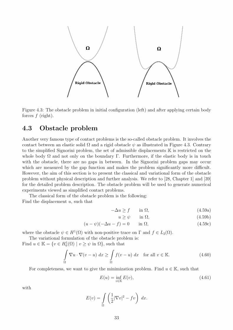
Figure 4.3: The obstacle problem in initial configuration (left) and after applying certain bodyforces f (right).

4.3 Obstacle problem

Another very famous type of contact problems is the so-called obstacle problem. It involves thecontact between an elastic solid Ω and a rigid obstacle ψ as illustrated in Figure 4.3. Contraryto the simplified Signorini problem, the set of admissible displacements K is restricted on thewhole body Ω and not only on the boundary Γ. Furthermore, if the elastic body is in touchwith the obstacle, there are no gaps in between. In the Signorini problem gaps may occurwhich are measured by the gap function and makes the problem significantly more difficult.However, the aim of this section is to present the classical and variational form of the obstacleproblem without physical description and further analysis. We refer to [28, Chapter 1] and [39]for the detailed problem description. The obstacle problem will be used to generate numericalexperiments viewed as simplified contact problems.

The classical form of the obstacle problem is the following:Find the displacement u, such that

−∆u ≥ f in Ω, (4.59a)

u ≥ ψ in Ω, (4.59b)

(u− ψ)(−∆u− f) = 0 in Ω, (4.59c)

where the obstacle ψ ∈ H1(Ω) with non-positive trace on Γ and f ∈ L2(Ω).The variational formulation of the obstacle problem is:

Find u ∈ K = v ∈ H10 (Ω) | v ≥ ψ in Ω, such that∫

Ω

∇u · ∇(v − u) dx ≥∫Ω

f(v − u) dx for all v ∈ K. (4.60)

For completeness, we want to give the minimization problem. Find u ∈ K, such that

E(u) = infv∈K

E(v), (4.61)

with

E(v) =

∫Ω

(1

2|∇v|2 − fv

)dx.

33

Chapter 5

Analysis of Variational Inequalities

The intent of this chapter is to present an analysis of variational inequalities in an abstract andgeneral form. As a motivation, we described the Signorini problem in the previous chapter,which led to a variational inequality. As a matter of fact, most contact problems in continuummechanics can be characterized by variational inequalities as well. The goal is to answerthe question about the existence of a unique solution for a wide range of different contactproblems obtaining general variational inequalities. Since many variational forms are related tominimization problems, we will investigate the characterization by minimization problems asa first step. We begin with introductory examples in the finite dimensional case following theideas of [19, Chapter 1]. Consequentially, we extend the observations of the finite dimensionalcase to an analysis on Hilbert spaces motivated by [1, Chapter 11], [13, Chapter 1], [18, Chapter3], [19, Chapter 3] and [26]. Using some results from the theory about minimization problems,a first statement about the existence and uniqueness of a solution can be derived. We extendour investigation to so-called elliptic variational inequalities, which are not necessarily relatedto minimization problems and answer the question about the unique solution as in [1, Chapter11] and [13, Chapter 1]. However, elliptic variational inequalities do not describe by far allkinds of contact problems, which gives us the opportunity to examine elliptic hemi-variationalinequalities. For this kind of problems, we refer to [6, Chapter 4], [11], [16, Chapter 2] and [34].The end of this chapter is left for an application of a contact problem with friction using theideas of hemi-variational inequalities, motivated by [6, Chapter 8] and [18, Chapter 10].

5.1 Introductory examples

We want to start with introductory examples in the finite dimensional case and we verify howminimization problems are related to variational inequalities. We refer to [19, Chapter 1] for avery clear introduction of variational inequalities.

Example 5.1. We consider the problem: Find x0 ∈ I = [a, b], such that

f(x0) = minx∈I

f(x),

where f is a real-valued smooth function. In order to find this minimum, three possible casescan occur:

1. If a < x0 < b, then f ′(x0) = 0.

2. If x0 = a, then f ′(x0) ≥ 0.

3. If x0 = b, then f ′(x0) ≤ 0.

34

These three possible cases can be easily summarized to

f ′(x0)(x− x0) ≥ 0 for all x ∈ I. (5.1)

We may call (5.1) a variational inequality in the finite dimensional case.

A further example for the d-dimensional case is the following.

Example 5.2. Let f be a smooth and real-valued function defined on the nonempty, closedand convex set K of the Euclidean d-dimensional space Rd. Again, we seek for x0 ∈ K, suchthat

f(x0) = minx∈K

f(x).

We assume that x0 ∈ K is the minimum point and let x ∈ K. Since K is convex, the segment(1− t)x0 + tx = x0 + t(x− x0) for t ∈ [0, 1], is also in K. Defining the function

ψ(t) = f(x0 + t(x− x0)), 0 ≤ t ≤ 1,

we can see, that the minimum is reached at t = 0. Therefore,

ψ′(0) = ∇f(x0) · (x− x0) ≥ 0 for any x ∈ K.

As a consequence, the point x0 satisfies the variational inequality: Find x0 ∈ K, such that

∇f(x0) · (x− x0) ≥ 0 for any x ∈ K. (5.2)

These examples were presented to give the first idea how to derive variational inequalitiesfrom minimization problems in the finite dimensional case.

5.2 Variational inequalities in Rd

In this section, we want to examine variational inequalities in the d-dimensional case. A bunchof nonlinear problems arising from variational inequalities can be solved by means of fixed pointapplications.

Definition 5.3. Let S be an arbitrary set and let F : S → S be a mapping on S. A pointx ∈ S is called fixed point of F , if

F (x) = x (5.3)

Usually, fixed point problems as (5.3) are solved in terms of contractions.

Definition 5.4. Let (S,m) be a metric space with metric function m. A mapping F : S → Sis a contraction mapping, if

m(F (x), F (y)) ≤ α m(x, y) for all x, y ∈ S, (5.4)

and for α ∈ [0, 1). If α = 1, the mapping is called non-expansive.

Only in terms of the contraction property we are able to guarantee a fixed point in completemetric spaces.

Theorem 5.5 (Contraction mapping theorem). Let S be a complete metric space and letF : S → S be a contraction mapping. Then there exists a unique fixed point of F .

35

Proof. See [22].

Remark 5.6. If F is non-expansive, Theorem 5.5 is generally not true. For example, rigidbody rotations do not have any fixed points, where S = [0, 1]× [0, 1]× [0, 1] and F (x) = Qx+ cfor all x ∈ S, with a constant rotation matrix Q (i.e. QTQ = I, det Q > 0) and a constantvector c.

Another fundamental theorem is Brouwer’s theorem, which ensures the existence of a fixedpoint on a closed ball.

Theorem 5.7 (Brouwer). Let F : B → B be a continuous mapping on a closed ball B ⊂ Rd.Then F admits at least one fixed point.

Proof. See [22].

Recalling Example 5.2, we receive from (5.2) that the minimum x0 fulfills

⟨∇f(x0), x− x0⟩ ≥ 0 for all x ∈ K,

where K is a nonempty, closed and convex subset in Rd and ⟨·, ·⟩ : (Rd)∗×Rd → R is the dualitypairing in Rd. In fact, the problem that we want to solve in the finite dimensional case is thefollowing.

Problem 5.8. Find x ∈ K, such that

⟨F (x), y − x⟩ ≥ 0 for all y ∈ K, (5.5)

where K ⊂ Rd is a nonempty, closed and convex subset and F : K → (Rd)∗ is continuous.

Remark 5.9. The dual space of any finite dimensional space Rd is the space itself, i.e. (Rd)∗ =Rd.

At this point, we are able to formulate a first statement about the uniqueness of variationalinequalities of the from (5.5). In general, the solution of a variational inequality need not to beunique.

Theorem 5.10. Let x and x′ be two different solutions of (5.5). If the condition

⟨F (x)− F (x′), x− x′⟩ > 0, (5.6)

is satisfied, then the solution of the variational inequality (5.5) in Rd is unique.

Proof. Let x, x′ ∈ K be two distinct solutions of (5.5), i.e.

⟨F (x), y − x⟩ ≥ 0, for all y ∈ K,⟨F (x′), y − x′⟩ ≥ 0, for all y ∈ K.

Choosing y = x′ and y = x and adding these two inequalities, we obtain that

⟨F (x)− F (x′), x− x′⟩ ≤ 0.

Since condition (5.6) holds with x = x′, we deduce that, there cannot be two different solutions.

In fact, condition (5.6) is used to define a strictly monotone mapping.

36

Definition 5.11. A mapping F : K → (Rd)∗ is monotone if

⟨F (x)− F (x′), x− x′⟩ ≥ 0 for all x, x′ ∈ K.

The mapping is called strictly monotone, if equality holds only for x = x′, i.e.

⟨F (x)− F (x′), x− x′⟩ > 0 for all x, x′ ∈ K and x = x′.

As we have seen in Theorem 5.10, the strict monotonicity guarantees the uniqueness of asolution of the variational inequality (5.5). Thus, for more general problems, e.g. variationalinequalities in Hilbert spaces, we need the monotonicity as a requirement for the uniquenessand, as we will see later, even for the existence. We want to investigate now, how variationalinequalities in Rd are related to minimization problems. As we have seen in the introductoryexamples, finding a minimum can be rewritten as a variational inequality.

Theorem 5.12. Let K ⊂ Rd be a nonempty, closed and convex subset, let f ∈ C1(K) and letx ∈ K be the solution of the minimization problem

f(x) = miny∈K

f(y). (5.7)

Then x ∈ K is also a solution of the variational inequality: Find x ∈ K, such that

(∇f(x), y − x) ≥ 0 for all y ∈ K. (5.8)

Proof. See Example 5.2.

With the help of convexity, we can prove the converse direction.

Theorem 5.13. Let f ∈ C1(K) be convex and let x ∈ K satisfy the inequality (5.8). Thenx ∈ K solves the minimization problem (5.7).

Proof. Let x ∈ K be a solution of (5.8). Since f is convex, we have by definition that

f(ty + (1− t)x) ≤ tf(y) + (1 + t)f(x) for all y ∈ K, t ∈ [0, 1]. (5.9)

Rewriting (5.9) yields

f(x+ t(y − x)) ≤ f(x) + t(f(y)− f(x)),

which gives

f(y) ≥ f(x) +f(x+ t(y − x))− f(x)

t, for all t ∈ (0, 1].

It follows that

f(y) ≥ f(x) + (∇f(x), y − x), (5.10)

as t→ 0. Since (5.8) holds, we deduce from (5.10) that

f(y) ≥ f(x) for all y ∈ K,

which concludes the proof.

By means of the convexity it can be shown that the gradient of a function is monotone.

37

Theorem 5.14. Let S ⊂ Rd be a open subset and let f : S → R be a continuously differen-tiable and convex (or strictly convex) function. Then F (x) = ∇f(x) is monotone (or strictlymonotone).

Proof. See [19, Chapter 1].

We want to conclude this section with a slightly changed version of Brouwer’s theorem usingthe property of the convexity.

Theorem 5.15 (Brouwer). Let K ⊂ Rd be a nonempty, compact and convex subset and letF : K → K be continuous. Then F admits a fixed point.

Proof. See [19, Chapter 1].

We will see later, that the fixed point theory is needed to prove the existence of a solutionfor variational inequalities as in (5.5). The proof will be done in the upcoming section for moregeneral variational inequalities, which covers the finite dimensional case as a consequence.

5.3 Elliptic variational inequalities in Hilbert spaces

In this section, we consider variational inequalities defined on a Hilbert space V . Throughoutthis chapter, we consider V to be a real Hilbert space, e.g. H1(Ω). As in [19, Chapter 1],we shortly want to examine projections on a nonempty, closed and convex subset K ⊂ V .Afterwards, we turn our attention to elliptic variational inequalities which represent one of themain parts of this work.

Lemma 5.16. Let K be a nonempty, closed and convex subset of V . Then for each x ∈ Vthere is a unique y ∈ K, called the projection point of x, such that

∥x− y∥ = infη∈K

∥x− η∥. (5.11)

The projection point can be written as

y = PKx.

Proof. See [19, Chapter 1].

The next theorem gives a characterization of the projection.

Theorem 5.17. Let K ⊂ V be a nonempty, closed and convex subset and let x ∈ V . Theny = PKx ∈ K is the projection of x on K if and only if

(y, η − y) ≥ (x, η − y) for all η ∈ K. (5.12)

Proof. See [19, Chapter 1].

As a consequence it can be obtained, that projection mapping is non-expansive.

Corollary 5.18. Let K ⊂ V be a nonempty, closed and convex subset and let x ∈ V . Then theprojection operator PK is non-expansive, i.e.

∥PKx− PKx′∥ ≤ ∥x− x′∥ for all x, x′ ∈ V.

Proof. See [19, Chapter 1].

38

5.3.1 Minimization problems of elliptic variational inequalities

We turn now our attention now to elliptic variational inequalities and want to determine howthey are related to minimization problems. In this section, we will follow the ideas of [1,Chapter 11], [13, Chapter 1], [18, Chapter 3] and [26]. We begin with some basic definitions,which denotes the properties of the linear functional F : K → R, and give a statement aboutthe connection between variational inequalities and minimization problems. As in the sectionbefore, we always consider K ⊂ V to be a nonempty, closed and convex subset of a Hilbertspace V and V ∗ denotes the dual space of V .

Definition 5.19 (Convexity). A functional F : K → R is called convex if and only if

F (tu+ (1− t)v) ≤ tF (u) + (1− t)F (v), (5.13)

for all u, v ∈ K and for all t ∈ [0, 1]. We say F is strictly convex if and only if

F (tu+ (1− t)v) < tF (u) + (1− t)F (v), (5.14)

for all u, v ∈ K with u = v and for all t ∈ (0, 1).

Definition 5.20 (Gateaux-differentiability). Let D be a normed space. A mapping F : K → Dis G-differentiable (or Gateaux-differentiable) at a point u ∈ K, if there exists a linear functionalDF (u) ∈ V ∗, such that

⟨DF (u), v⟩ = limt→0

F (u+ tv)− F (u)

t, (5.15)

for all v ∈ K, where ⟨·, ·⟩ denotes the duality paring on V ∗ × V . We call DF (u) the Gateauxderivative (G-derivative) of F at u and ⟨DF (u), v⟩ the Gateaux derivative of F at point u indirection v. The second Gateaux derivative is defined as

⟨D2F (u)(v), w⟩ = limt→0

⟨DF (u+ tv), w⟩ − ⟨DF (u), w⟩t

,

for all u, v, w ∈ K.

Definition 5.21 (Lower and upper semi-continuity). A functional F : K → R is called lowersemi-continuous on K if for any sequence uk ⊂ K with the property that uk converges tou ∈ K, i.e. ∥uk − u∥ → 0 as k → ∞, we have

lim infk→∞

F (uk) ≥ F (u). (5.16)

The function is called upper semi-continuous if

lim supk→∞

F (uk) ≤ F (u), (5.17)

for any uk → u ∈ K. If F is lower and upper semi-continuous, then F is continuous. Replacingthe strong convergence of the sequence uk by the weak convergence, i.e.

limk→∞

⟨f, uk⟩ = ⟨f, u⟩ for all f ∈ V ∗,

then we call F weakly lower or weakly upper semi-continuous, respectively.

Remark 5.22. The lower or upper semi-continuity implies the weakly lower or weakly uppersemi-continuity.

39

The next two theorems clarify the connection between the definitions we introduced andgive some helpful properties we may use later.

Theorem 5.23. Let F : K → R satisfy the following conditions:

i) F is convex.

ii) F is G-differentiable on K.

Then F is weakly lower semi-continuous on K.

Proof. See [20, Chapter 3].

Theorem 5.24. Let F : K → R be G-differentiable. Then the following statements are equiv-alent.

i) F is convex.

ii) ⟨DF (u)−DF (v), u− v⟩ ≥ 0, for all u, v ∈ K.

iii) F (v) ≥ F (u) + ⟨DF (u), v − u⟩, for all u, v ∈ K.

Moreover, if F is twice G-differentiable, then the above statements are also equivalent to

iv) ⟨D2F (u)(v), v⟩ ≥ 0, for all v ∈ K.

Proof. See [11, Chapter 1].

Remark 5.25. In fact, we have proven the equivalence of statement i) and iii) of Theorem5.24 in the proof of Theorem 5.13 for the finite dimensional case.

We are now able to present the relation between variational inequalities and minimizationproblems in terms of the above definitions and theorems.

Theorem 5.26. Let K be a nonempty, closed and convex subset of V and let F : K → R be aG-differentiable functional. If u ∈ K is a minimizer of F in K, i.e. F (u) = minv∈K F (v), thenu may be characterized in one of the following ways:

i) u ∈ K is a solution of the variational inequality

⟨DF (u), v − u⟩ ≥ 0 for all v ∈ K.

ii) If u is in the interior of K, i.e. u ∈ int K, then it solves

⟨DF (u), v⟩ = 0 for all v ∈ K.

iii) If K is a nonempty, closed and convex cone with vertex w, then u solves

⟨DF (u), u− w⟩ = 0 and ⟨DF (u), v − w⟩ ≥ 0 for all v ∈ K.

iv) If K is a linear subspace of V , then u solves

⟨DF (u), v⟩ = 0 for all v ∈ K.

Proof. Follows from Theorem 5.27 with j = 0.

40

The latter theorem can be formulated for more general variational inequalities. For thispurpose, we extend the variational inequality with an functional j : K → R.

Theorem 5.27. Let K be a nonempty, closed and convex subset of V , let F : K → R andj : K → R be two convex functionals and let F be G-differentiable. Then u ∈ K solves theminimization problem

F (u) + j(u) = infv∈K

[F (v) + j(v)] , (5.18)

if and only if u ∈ K solves

⟨DF (u), v − u⟩+ j(v)− j(u) ≥ 0 for all v ∈ K, (5.19a)

⟨DF (v), v − u⟩+ j(v)− j(u) ≥ 0 for all v ∈ K. (5.19b)

Moreover, if K is a subspace of V and j = 0 almost everywhere, then the inequality (5.19a)reduces to an equality, i.e. u ∈ K solves

⟨DF (u), v⟩ = 0 for all v ∈ K. (5.20)

Proof. First, we want to prove that a solution of (5.18) solves (5.19a). Let u ∈ K be the solutionof (5.18). Due to the convexity of K we have that tv + (1 − t)u = u + t(v − u) ∈ K for anyv ∈ K and any t ∈ (0, 1). Hence,

F (u) + j(u) ≤ F (u+ t(v − u)) + j(u+ t(v − u))

= F (u+ t(v − u)) + j((1− t)u+ tv)

≤ F (u+ t(v − u)) + (1− t)j(u) + tj(v),

where the last inequality follows from the convexity of j. Subtracting the left hand side fromthe right hand side gives

F (u+ t(v − u))− F (u) + tj(u) + tj(v) ≥ 0. (5.21)

Dividing (5.21) by t yields

F (u+ t(v − u))− F (u)

t+ j(u) + j(v) ≥ 0 for all t ∈ (0, 1).

Letting t→ 0 and using the fact that F is G-differentiable we obtain (5.19a).The other way round, we assume that u ∈ K is a solution of (5.19a). Since F is convex, we

can write with the help of Theorem 5.24 that

F (v) ≥ F (u) + ⟨DF (u), v − u⟩ for all v ∈ K.

Thus,

F (v) + j(v) ≥ F (u) + j(v) + ⟨DF (u), v − u⟩. (5.22)

Since u satisfies (5.19a), we can write j(v) + ⟨DF (u), v − u⟩ ≥ j(u) . Hence, it follows from(5.22) that

F (v) + j(v) ≥ F (u) + j(u) for all v ∈ K,

which gives (5.18).

41

If j = 0 almost everywhere, (5.19a) becomes to

⟨DF (u), v − u⟩ ≥ 0.

If K is a subspace we can choose v = w + u for any w ∈ K, which gives

⟨DF (u), w⟩ ≥ 0 for all w ∈ K. (5.23)

Due to the fact that K is a subspace of V , for any w ∈ K also −w ∈ K, therefore

⟨DF (u), w⟩ ≤ 0 for all w ∈ K. (5.24)

(5.23) and (5.24) together yield (5.20).It remains to show the characterization of (5.19a) and (5.19b), which directly follows from

the Minty Lemma 5.48 with A = DF .

Remark 5.28. As we can see in the last proof, the convexity of K is essential. However, theexistence of a solution has been assumed. In order to formulate an existence and uniquenessstatement about the solution of variational inequalities stronger assumptions must be required,which will be the topic of the next section.

At this point we can use a result from minimization theory to give a first statement aboutthe unique solution of the minimization problem (5.18). An adjusted version of the generalizedWeierstrass theorem indicates a good result.

Theorem 5.29 (Generalized Weierstrass minimization theorem). Let F : K → R be a convexand lower semi-continuous functional defined on a nonempty, closed and convex subset K ⊂ V .Moreover, let one of the following conditions holds:

i) K is bounded.

ii) F is coercive on K, i.e.

lim∥v∥→∞

F (v) = +∞.

Then the problem: Find u ∈ K, such that

F (u) = infv∈K

F (v),

has at least one solution. Furthermore, if F is strictly convex, then the solution is unique.

Proof. [47, Chapter 1]

Remark 5.30. For a bunch of problems, the subset K is unbounded and, therefore, in mostsituations the second property must be proven. In order to show that F is coercive on K, anestimate of the form

F (v) ≥ C0∥v∥α − C1∥v∥β, (5.25)

with C0, C1 > 0 and α > β can be used.

The generalized Weierstrass minimization theorem gives the existence of a solution for theminimization problem (5.18) if we are able to guarantee one of the assumptions. In addition, itfollows directly from Theorem 5.27 that the variational inequality (5.19a) admits a solution too.Considering now problems with a bilinear form a we can make use of the latest two theoremsto show the following result.

42

Theorem 5.31. Let K ⊂ V be a nonempty, closed and convex subset. Assume that a : V ×V →R is a bounded, symmetric and V -elliptic bilinear form, l ∈ V ∗ and j : K → R is convex andlower semi-continuous on K. Then the minimization problem: Find u ∈ K, such that

E(u) = infv∈K

E(v), (5.26)

with

E(v) =1

2a(v, v) + j(v)− l(v),

has a unique solution. Moreover, u ∈ K is a solution of the minimization problem if and onlyif u ∈ K is a solution of

a(u, v − u) + j(v)− j(u) ≥ l(v − u) for all v ∈ K. (5.27)

Proof. Follows from Theorem 5.29, since condition ii) is valid for elliptic bilinear forms withthe help of Lemma 5.45 and Theorem 5.27 with ⟨DF (u), v − u⟩ = a(u, v − u) − l(v − u). Seealso [1, Chapter 11].

Remark 5.32. In the latest proof, the auxiliary Lemma 5.45 is needed for the functional j, inorder to guarantee property ii) of Theorem 5.29. Lemma 5.45 will be introduced in the sequel.

At this point, we want to apply Theorem 5.31 on the two examples, which we have in-troduced in the previous chapter. We start with the obstacle problem and move on with thesimplified Signorini problem.

Example 5.33 (Obstacle problem). We have already seen that the set of admissible displace-ments of the obstacle problem (4.59) is defined as

K = v ∈ H10 (Ω) | v ≥ ψ in Ω ⊂ V = H1

0 (Ω),

which is nonempty, since the function max0, ψ is an element in K with ψ ∈ H1(Ω) withnon-positive trace, c.f. [28, Chapter 4]. This set is also closed and convex, c.f. [13, Chapter 2].The bilinear form of the obstacle problem is defined as

a(u, v) =

∫Ω

∇u · ∇v dx.

Indeed, it is bounded, symmetric and elliptic with respect to H10 (Ω). The right hand side of

the obstacle problem is

l(v) =

∫Ω

fv dx.

In fact, l is bounded and l ∈ V ∗. Furthermore, j(v) = 0 for all v ∈ H10 (Ω). Thus, we can apply

Theorem 5.31 to obtain that the variational inequality: Find u ∈ K, such that∫Ω

∇u · ∇(v − u) dx ≥∫Ω

f(v − u) dx for all v ∈ K,

and the corresponding minimization problem: Find u ∈ K, such that

E(u) = infv∈K

E(v),

with

E(v) =

∫Ω

(1

2|∇v|2 − fv

)dx,

have a unique solution.

43

Example 5.34 (Simplified Signorini problem). We similarly conclude, that the set of admissibledisplacements K = v ∈ H1(Ω) | v ≥ 0 on Γ = ∂Ω ⊂ V = H1(Ω) of the simplified Signoriniproblem (4.25) is nonempty, closed and convex. Furthermore, the bilinear form

a(u, v) =

∫Ω

∇u · ∇v + uv dx

is bounded, symmetric and elliptic with respect to H1(Ω), the right hand side

l(v) =

∫Ω

fv dx+

∫Γ

gv ds,

is bounded and l ∈ V ∗, and j(v) = 0 for all v ∈ H1(Ω). Hence, by Theorem 5.31, the variationalinequality: Find u ∈ K, such that∫

Ω

∇u · ∇(v − u) + u(v − u) dx ≥∫Ω

f(v − u) dx+

∫Γ

g(v − u) ds for all v ∈ K,

and the corresponding minimization problem: Find u ∈ K , such that

E(u) = infv∈K

E(v),

where

E(v) =

∫Ω

(1

2(|∇v|+ v)2 − fv

)dx−

∫Γ

gv ds,

have a unique solution.

5.3.2 Existence and uniqueness results of variational inequalities

In Theorem 5.31 the variational inequality (5.27) is associated with minimization problems.The aim of this section is to prove the existence and uniqueness of a solution for variationalinequalities not necessarily related to minimization problems following the ideas of [1, Chapter11] and [13, Chapter 1]. For this purpose, let V be a real Hilbert space with inner product(·, ·) and norm ∥ · ∥ and let K ⊂ V be a nonempty, closed and convex subset. We consider thefollowing variational inequality.

Problem 5.35. Find u ∈ K, such that

(A(u), v − u) + j(v)− j(u) ≥ (f, v − u) for all v ∈ K, (5.28)

where A : V → V is an operator, j : K → R is a functional and f ∈ V .

The operator needs to satisfy some conditions in order to prove the existence and uniquenessof (5.28).

Definition 5.36 (Monotonicity). Let V be a real Hilbert space. An operator A : V → V iscalled monotone if

(A(u)− A(v), u− v) ≥ 0 for all u, v ∈ V.

The operator A is strongly monotone if there is exists a constant c0 > 0, such that

(A(u)− A(v), u− v) ≥ c0∥u− v∥2 for all u, v ∈ V.

44

Definition 5.37 (Lipschitz continuity). Let V be a real Hilbert space. An operator A : V → Vis Lipschitz continuous if there exists a constant L > 0, such that

∥A(u)− A(v)∥ ≤ L∥u− v∥ for all u, v ∈ V.

We are now ready to formulate and prove the main theorem ensuring a unique solution ofthe variational inequality (5.28).

Theorem 5.38. Let V be a real Hilbert space and K ⊂ V a nonempty, closed and convex subset.Moreover, let A : V → V be strongly monotone and Lipschitz continuous and let j : K → R bea convex and lower semi-continuous functional. Then the elliptic variational inequality (5.28),i.e.: Find u ∈ K, such that

(A(u), v − u) + j(v)− j(u) ≥ (f, v − u) for all v ∈ K,

has a unique solution for any f ∈ V and the solution is Lipschitz continuously depending on f .

Proof. Firstly, we prove the uniqueness of the solution. Assume that there are two solutionsu1, u2 ∈ K for (5.28). If we choose v = u2 for the first inequality and v = u1 for the secondinequality, then the following holds.

(A(u1), u2 − u1) + j(u2)− j(u1) ≥ (f, u2 − u1),

(A(u2), u1 − u2) + j(u1)− j(u2) ≥ (f, u1 − u2).

Adding these two inequalities yields

−(A(u1)− A(u2), u1 − u2) ≥ 0,

or equivalently

(A(u1)− A(u2), u1 − u2) ≤ 0. (5.29)

Since A is a strongly monotone operator, we deduce from (5.29) that

0 ≥ (A(u1)− A(u2), u1 − u2) ≥ c0∥u1 − u2∥2 ≥ 0, (5.30)

for c0 ≥ 0. It follows from (5.30) that

∥u1 − u2∥ = 0,

from where we deduce that u1 = u2, which proves the uniqueness.In order to prove the existence of a solution, we convert the variational inequality into an

equivalent fixed-point problem. For any θ > 0, the equivalent fixed point problem is: Findu ∈ K, such that

(u,v − u) ≥ (u, v − u) + θ ((f, v − u)− (A(u), v − u)− j(v) + j(u)) , (5.31)

for all v ∈ K. Problem (5.31) can be equivalently rewritten as: Find u ∈ K, such that

(u, v − u) + θj(v)− θj(u) ≥ (u, v − u)− θ(A(u), v − u) + θ(f, v − u), (5.32)

for all v ∈ K. Now, for any u ∈ K we consider the problem: Find w ∈ K, such that

(w, v − w) + θj(v)− θj(w) ≥ (u, v − w)− θ(A(u), v − w) + θ(f, v − w) for all v ∈ K.(5.33)

45

(5.33) is equivalent to the minimization problem: For a given u ∈ K, find w ∈ K, such that

E(w) = infv∈K

E(v), (5.34)

where

E(v) =1

2∥v∥2 + θj(v)− (u, v) + θ(A(u), v)− θ(f, v).

By the auxiliary Lemma 5.45, there exists a continuous functional lj ∈ V ∗ and a constantcj > 0, such that

j(v) ≥ lj(v) + cj for all v ∈ V.

Applying Theorem 5.31, where

a(w, v − w) = (w, v − w),

j(w) = θj(w),

l(v − w) = (u, v − w)− θ(A(u), v − w) + θ(f, v − w),

we obtain that (5.34), and hence (5.33), has a unique solution w ∈ K, since property ii) is validdue to the coercivity of a and Lemma 5.45.We define now for each θ > 0, the mapping Pθ : K → K by w = Pθu, where w is the uniquesolution of (5.33). Obviously, a fixed point of the mapping Pθ is a solution of our problem(5.32). We want to prove, that for sufficiently small θ > 0, Pθ : K → K is a contraction and,therefore, by the Banach’s fixed point theorem 2.14, the inequality (5.32) has a unique solution.For any u1, u2 ∈ K, let w1 = Pθu1 and w2 = Pθu2. Then

(w1, w2 − w1) + θj(w2)− θj(w1) ≥ (u1, w2 − w1)− θ(A(u1), w2 − w1) + θ(f, w2 − w1),

(w2, w1 − w2) + θj(w1)− θj(w2) ≥ (u2, w1 − w2)− θ(A(u2), w1 − w2) + θ(f, w1 − w2).(5.35)

Adding the two inequalities in (5.35) and simplifying yields

∥w1 − w2∥2 ≤ (u1 − u2 − θ(A(u1)− A(u2)), w1 − w2).

By the Cauchy-Schwarz inequality we get

∥w1 − w2∥ ≤ ∥u1 − u2 − θ(A(u1)− A(u2))∥. (5.36)

We see that

∥u1 − u2 − θ(A(u1)− A(u2))∥2

= ∥u1 − u2∥2 − 2θ(A(u1)− A(u2), u1 − u2) + θ2∥A(u1)− A(u2)∥2

≤ (1− 2c0θ + L2θ2)∥u1 − u2∥2,(5.37)

where the last estimate follows from the strong monotonicity with negative sign and the Lips-chitz continuity of A. Thus, (5.36) yields with the help of (5.37) that

∥Pθu1 − Pθu2∥ = ∥w1 − w2∥ ≤ (1− 2c0θ + L2θ2)12∥u1 − u2∥.

Hence, the mapping Pθ is a contraction for θ ∈ (0, 2c0L2 ) and therefore, by Banach’s fixed point

theorem, Pθ has a unique fixed point, i.e. u = Pθu. Consequently, (5.31) has a unique fixedpoint, which means that the equivalent variational inequality (5.28) has a unique solution u ∈ K.

46

Lastly, we want to prove the Lipschitz continuous dependency of f . Therefore, let f1, f2 ∈ Vand let u1, u2 ∈ K denote the corresponding solutions of the variational inequality (5.28). Thenchoosing v = u2 for the first inequality and v = u1 for the second inequality we get

(A(u1), u2 − u1) + j(u2)− j(u1) ≥ (f1, u2 − u1),

(A(u2), u1 − u2) + j(u1)− j(u2) ≥ (f2, u1 − u2).

Adding these two inequalities yields

(A(u1)− A(u2), u1 − u2) ≤ (f1 − f2, u1 − u2).

Using again the strong monotonicity and the Lipschitz continuity of A gives

∥u1 − u2∥ ≤ L

c0∥f1 − f2∥,

which means that the solution depends Lipschitz continuously on f.

Remark 5.39. Following the proof of Theorem 5.38, it can be seen that the assumptions onthe operator A can be weakened. Firstly, the strong monotonicity and the Lipschitz continuityneed only to be assumed on the subset K and not over the whole space V . Nevertheless, thereis usually a natural extension of A to an operator A0 on V which fulfills the conditions on thewhole space.

Remark 5.40. The results about the solution in Theorem 5.38 are valid for elliptic variationalinequalities of the form (5.28), i.e. with a special right hand side (f, v) for f ∈ V . By theRiesz representation theorem, c.f. [6, Chapter 4], there exists a unique f ∈ V , such that forany l ∈ V ∗

l(v) = (f, v) for all v ∈ V.

This makes Theorem 5.38 valid for elliptic variational inequalities of the form

(A(u), v − u) + j(v)− j(u) ≥ l(v − u) for all v ∈ K. (5.38)

In the literature, variational inequalities are grouped into two popular characterizations.We differentiate between elliptic variational inequalities of the first kind and elliptic variationalinequalities of the second kind. If the functional j(v) = 0 for all v ∈ V , then the variationalinequality reduces to a first kind inequality,

(A(u), v − u) ≥ (f, v − u) for all v ∈ K. (5.39)

The obstacle problem (4.60) is an example of elliptic variational inequalities of the first kind.Moreover, they are characterized by the feature that the problem is posed over a convex subsetK. In fact, if K is a subspace of V , then the variational inequality becomes to a variationalequality, as we have similarly seen in Theorem 5.27. As a corollary of Theorem 5.38 we havethe following result for elliptic variational inequalities of the first kind.

Corollary 5.41. Let K ⊂ V be a nonempty, closed and convex subset and let A : V → Vbe strongly monotone and Lipschitz continuous. Then for any f ∈ V , the elliptic variationalinequality (5.39) has a unique solution u ∈ K, which depends Lipschitz continuously on f .

Remark 5.42. Corollary 5.41 is a generalization of the Lax-Milgram Lemma.

47

The functional j in (5.28) is defined on the subset K. However, we can extend the functionalj to V , using the same symbol for its extension. The extension is

j(v) =

j(v) if v ∈ K,+∞ if v ∈ V \K.

(5.40)

Furthermore, we need the property of a proper functional.

Definition 5.43. Let V be a real Hilbert space. We call a functional j : V → R = R ∪ ±∞proper if j(v) > −∞ for all v ∈ V and j(v) = +∞ for at least one v ∈ V .

Remark 5.44. The extension j : V → R is lower semi-continuous if and only if K ⊂ V isclosed and j : K → R is lower semi-continuous.

Theorem 5.38 can be now stated without using a convex subset K explicitly. If we use theextension of j (5.40), then the variational inequality (5.28) changes to an elliptic variationalinequality of the second kind: Find u ∈ V , such that

(A(u), v − u) + j(v)− j(u) ≥ (f, v − u) for all v ∈ V. (5.41)

We need the following assisting lemma in order to ensure a unique solution for the variationalinequality of the second kind (5.41).

Lemma 5.45. Let V be a normed space and let j : V → R be a proper, convex and lowersemi-continuous functional. Then there exists a continuous linear functional lj ∈ V ∗ and aconstant cj ∈ R such that

j(v) ≥ lj(v) + cj for all v ∈ V.

Proof. See [1, Chapter 11]

Corollary 5.46. Let A : V → V be strongly monotone and Lipschitz continuous and letj : V → R be a proper, convex and lower semi-continuous functional on V . Then for anyf ∈ V , the elliptic variational inequality of the second kind (5.41) has a unique solution.

Remark 5.47. Usually, the functional j is a non-differential functional and causes difficultieswhen it comes to solving the variational inequality numerically. As an example, variationalinequalities derived from frictional contact problems contain non-differential expressions. Wewant to give an example about a contact problem with friction at the end of this chapter.

An important property for variational inequalities is the so called Minty Lemma, whichalready occurred in the proof of Theorem 5.27. This Lemma can be seen as a symmetrystatement about variational inequalities. In addition, the Minty Lemma is very useful forconvergence results of numerical solutions, which we will examine in the next chapter.

Theorem 5.48 (Minty Lemma). Let K ⊂ V be a nonempty, closed and convex subset. More-over, let A : V → V be strongly monotone and Lipschitz continuous and let j : K → R be convexand lower semi-continuous. Then u ∈ K is a solution of the variational inequality (5.28) if andonly if u ∈ K is a solution of

(A(v), v − u) + j(v)− j(u) ≥ (f, v − u) for all v ∈ K. (5.42)

48

Proof. We first assume that u ∈ K satisfies (5.28). The monotonicity of A yields

(A(u)− A(v), u− v) ≥ c0∥u− v∥2 ≥ 0,

which means that

(A(u), u− v) ≥ (A(v), u− v),

or equivalently

(A(v), v − u) ≥ (A(u), v − u),

for all v ∈ K. Hence, u satisfies (5.42).Conversely, assume that u ∈ K is a solution of (5.42). For any v ∈ K and t ∈ (0, 1), also

u+ t(v − u) ∈ K. Using now u+ t(v − u) instead of v in (5.42), we get

(A(u+ t(v − u)), u+ t(v − u)− u) + j(u+ t(v − u))− j(u) ≥ (f, u+ t(v − u)− u),

from where we get

t(A(u+ t(v − u)), v − u) + j(tv + (1− t)u)− j(u) ≥ t(f, v − u). (5.43)

Applying the convexity of the functional j on (5.43), we deduce that

t(A(u+ t(v − u)), v − u) + tj(v)− tj(u) ≥ t(f, v − u),

which is equivalent to

(A(u+ t(v − u)), v − u) + j(v)− j(u) ≥ (f, v − u).

As t→ 0, we obtain (5.28).

In many applications the operator A corresponds to a bilinear form on the space V , whichallows us to write

(A(u), v) = a(u, v) for all u, v ∈ V.

Using the Ritz functional l ∈ V ∗, we deduce the following corollary about variational in-equalities with bilinear forms as a consequence of Theorem 5.38.

Corollary 5.49. Let K ⊂ V be a nonempty, closed and convex subset. Moreover, let a :V × V → R be a continuous and V -elliptic bilinear form, let l ∈ V ∗ and let j : K → R bea convex and lower semi-continuous functional. Then each of the following elliptic variationalinequalities: Find u ∈ K, such that

a(u, v − u) + j(v)− j(u) ≥ l(v − u) for all v ∈ K; (5.44)

Find u ∈ K, such that

a(u, v − u) ≥ l(v − u) for all v ∈ K; (5.45)

Find u ∈ V , such that

a(u, v − u) + j(v)− j(u) ≥ l(v − u) for all v ∈ V, (5.46)

has a unique solution. In addition, the solution depends Lipschitz continuously on l.

We have already seen that the obstacle problem (4.60) and the simplified Signorini problem(4.44) can be solved uniquely. With the help of Theorem 5.49 the existence and uniquenessof these problems are guaranteed without knowing the corresponding minimization problemexplicitly.

49

5.4 Elliptic hemi-variational inequalities

We have always spoken about elliptic variational inequalities of the form (5.28) so far. Infact, many applications require more general observations of variational inequalities, where onetype is called elliptic hemi-variational inequalities. For example, contact problems with frictionrequire the usage of elliptic hemi-variational inequalities. This kind of inequalities allow thefunctional j to depend explicitly on the solution of the convex subsetK. As in the section before,we want to give an statement about a unique solution of elliptic hemi-variational inequalitiesfollowing the ideas of [6, Chapter 4] and [34].

Remark 5.50. In the literature, the variational inequality (5.28) is also referred to as ellipticquasi-variational inequality. However, we want to stick to our introduced designation throughoutthis chapter.

As before, let V and V ∗ denote a Hilbert space and its dual space, e.g. V = H1(Ω) andV ∗ = H−1(Ω), with their respective norms ∥ · ∥ and ∥ · ∥∗. The set K is a nonempty, closed andconvex subset of V . Furthermore, we consider an operator A : V → V ∗ defined on V into thedual space of V ∗. Throughout this section, we consider the following elliptic hemi-variationalinequality: Find u ∈ K, such that

⟨A(u), v − u⟩+ j(u, v)− j(u, u) ≥ l(v − u) for all v ∈ K, (5.47)

where j : V × V → (−∞,+∞] is a functional, l ∈ V ∗ and ⟨·, ·⟩ : V ∗ × V → R is the dualityproduct between V ∗ and V . Note that we mean the duality product ⟨l, v⟩ when we write l(v)for l ∈ V ∗.

Remark 5.51. Note that for the variational inequality (5.28) in the previous chapter, theoperator A : V → V is defined on the Hilbert space V and not on its dual space V ∗. However,by the Riesz representation theorem, c.f. [6, Chapter 4], there is an isomorphism R : V ∗ → V ,called the Riesz mapping, such that

A = RA

where A : V → V ∗ is defined on the dual space V ∗. Thus, the statements in the previouschapter are also valid for the operator A (with technical adaptions). In the sequel, we use forelliptic variational inequalities of the form (5.28) the operator A defined on V , i.e. A : V → V .For elliptic hemi-variational inequalities (5.47), we use the operator A, denoting it by A, i.e.A : V → V ∗.

In order to answer the question about a unique solution of elliptic hemi-variational inequal-ities (5.47) we need to introduce some essential definitions.

Definition 5.52 (Hemi-continuity). An operator A : V → V ∗ is called hemi-continuous if forall u, v ∈ V and t ∈ [0, 1] the mapping

t→ ⟨A((1− t)u+ tv), u− v⟩ (5.48)

is continuous.

Definition 5.53. An operator A : V → V ∗ is called monotone if

⟨A(u)− A(v), u− v⟩ ≥ 0 for all u, v ∈ V.

The operator A is called strongly monotone if there exists a constant c0 > 0, such that

⟨A(u)− A(v), u− v⟩ ≥ c0∥u− v∥2 for all u, v ∈ V.

50

Furthermore, we need some essential properties for the functional j : V × V → (−∞,+∞]in order to guarantee a unique solution of (5.47). Firstly, we assume that there exists a constantk < c0, such that

|j(u1, v1) + j(u2, v2)− j(u1, v2)− j(u2, v1)| ≤ k∥u1 − u2∥∥v1 − v2∥, (5.49)

for all u1, u2, v1, v2 ∈ K, where c0 is the constant coming from the strong monotonicity of A. Inaddition, we always consider the functional j(u, ·) : V → (−∞,+∞] to be proper, convex andlower semi-continuous for every u ∈ V .

Before we state the main theorem about the existence of a unique solution for (5.47), werecall the generalized Weierstrass Minimization Theorem 5.29 and give an adjusted version ofit, called the Coercivity Theorem.

Theorem 5.54 (Coercivity Theorem). Let K ⊂ V be a nonempty, closed and convex subset,let j : K → R = R∪−∞,+∞ be a proper, lower semi-continuous and convex functional andlet A : V → V ∗ be a monotone and hemi-continuous operator. If one of the following conditionsis satisfied

K is bounded, (5.50)

or, there exists a v0 ∈ K, such that

lim∥v∥→+∞v∈K

⟨A(v), v − v0⟩+ j(v)− j(v0)

∥v∥= +∞, (5.51)

then there exists at least one solution u ∈ K of the variational inequality

⟨A(u), v − u⟩+ j(v)− j(u) ≥ l(v − u) for all v ∈ K. (5.52)

In addition, if the functional j is strictly convex, i.e.

j(tu+ (1− t)v) < tj(u) + (1− t)j(v) for all u, v ∈ V, t ∈ (0, 1), and u = v, (5.53)

or A is strictly monotone, i.e.

⟨A(u)− A(v), v − u⟩ > 0 for all u, v ∈ V, and u = v, (5.54)

then the solution of the elliptic variational inequality (5.52) is unique.

Proof. See [6, Chapter 4].

As a consequence of the Coercivity Theorem 5.54 the following statement holds.

Lemma 5.55. Let K ⊂ V be a nonempty, closed and convex subset, let j : K → R be a proper,lower semi-continuous and convex functional and let A : V → V ∗ be a strongly monotone andhemi-continuous operator. Then the elliptic variational inequality (5.52) has a unique solutionu ∈ K.

Proof. See [6, Chapter 4].

Lastly, we need an auxiliary lemma, which is comparable to Lemma 5.45.

Lemma 5.56. Let V be a normed space and let j : V × V → (−∞,+∞] be a functional, suchthat for every u ∈ V , the functional j(u, ·) : V → (−∞,+∞] is proper, convex and lower semi-continuous. Then there exists a continuous linear functional lj = lj(u) ∈ V ∗ and a constantcj ∈ R, such that

j(u, v) ≥ lj(v) + cj for all v ∈ V.

51

Proof. See [6, Chapter 4]

Now we are able to state the existence and uniqueness theorem for hemi-variational inequal-ities of the form (5.47).

Theorem 5.57. Let V be a real Hilbert space and K ⊂ V a nonempty, closed and convexsubset. Moreover, let A : V → V ∗ be a strongly monotone and hemi-continuous operator andlet j : V × V → (−∞,+∞] be a functional, such that (5.49) is satisfied and for every u ∈ V ,the functional j(u, ·) : V → (−∞,+∞] is proper, convex and lower semi-continuous. Then theelliptic hemi-variational inequality (5.47), i.e.: Find u ∈ K, such that

⟨A(u), v − u⟩+ j(u, v)− j(u, u) ≥ l(v − u) for all v ∈ K,

has a unique solution for any l ∈ V ∗, which depends Lipschitz continuously on l.

Proof. Firstly, we prove the uniqueness of the solution u ∈ K for the elliptic hemi-variationalinequality (5.47). Assume that there exist two different solutions u1, u2 ∈ K for (5.47). If wechoose v = u2 for the first inequality and v = u2 for the second inequality, then the followingholds.

⟨A(u1), u2 − u1⟩+ j(u1, u2)− j(u1, u1) ≥ l(u2 − u1),

⟨A(u2), u1 − u2⟩+ j(u2, u1)− j(u2, u2) ≥ l(u1 − u2).(5.55)

Adding the two inequalities in (5.55) yields

−⟨A(u1)− A(u2), u1 − u2⟩ − j(u1, u1)− j(u2, u2) + j(u1, u2) + j(u2, u1) ≥ 0,

which is equivalent to

⟨A(u1)− A(u2), u1 − u2⟩+ j(u1, u1) + j(u2, u2)− j(u1, u2)− j(u2, u1) ≤ 0. (5.56)

Using the strong monotonicity of A and property (5.49) of j in (5.56) gives for c0 < k

0 ≥ ⟨A(u1)− A(u2), u1 − u2⟩+ j(u1, u1) + j(u2, u2)− j(u1, u2)− j(u2, u1)

≥ ⟨A(u1)− A(u2), u1 − u2⟩ − |j(u1, u1) + j(u2, u2)− j(u1, u2)− j(u2, u1)|≥ c0∥u1 − u2∥2 − k∥u1 − u2∥2 = (c0 − k)∥u1 − u2∥2 ≥ 0.

Hence,

0 ≥ ∥u1 − u2∥2 ≥ 0,

therefore

∥u1 − u2∥ = 0,

holds, which proves the uniqueness of the solution.Secondly, we prove that there exists a solution for the hemi-variational inequality (5.47) by

using the Coercivity Theorem 5.54. We want to verify condition (5.51) of Theorem 5.54. Forthis purpose, let v, v0 ∈ K. Then

⟨A(v), v − v0⟩∥v∥

=⟨A(v)− A(v0) + A(v0), v − v0⟩

∥v∥=

⟨A(v)− A(v0), v − v0⟩∥v∥

+⟨A(v0), v − v0⟩

∥v∥

≥ c0∥v − v0∥2

∥v∥− ∥A(v0)∥∗∥v∥+ ∥A(v0)∥∗∥v0∥

∥v∥,

(5.57)

52

where the last estimate follows from the strong monotonicity of the operator A and the Cauchy-Schwarz inequality with negative sign. Further, we have for the last expression in (5.57) that

c0∥v − v0∥2

∥v∥− ∥A(v0)∥∗∥v∥+ ∥A(v0)∥∗∥v0∥

∥v∥

=c0∥v∥2 − 2c0∥v∥∥v0∥+ c0∥v0∥2

∥v∥− ∥A(v0)∥∗∥v∥

∥v∥+

∥A(v0)∥∗∥v0∥∥v∥

= c0∥v∥ − 2c0∥v0∥ − ∥A(v0)∥∗ +c0∥v0∥2

∥v∥− ∥A(v0)∥∗∥v0∥

∥v∥.

(5.58)

(5.57) and (5.58) together yield

⟨A(v), v − v0⟩∥v∥

≥ c0∥v∥ − 2c0∥v0∥ − ∥A(v0)∥∗ +c0∥v0∥2

∥v∥− ∥A(v0)∥∗∥v0∥

∥v∥, (5.59)

for all v, v0 ∈ K. Hence,

lim∥v∥→+∞

⟨A(v), v − v0⟩∥v∥

= +∞. (5.60)

Using now Lemma 5.56 we deduce that there exists a functional lj ∈ V ∗ and a constant cj ∈ R,such that for any w ∈ K

j(w, v) ≥ lj(v) + cj ≥ −∥lj∥∗∥v∥+ cj for all v ∈ K. (5.61)

Thus, with the help of (5.60) and (5.61) it follows that

lim∥v∥→+∞

⟨A(v), v − v0⟩+ j(w, v)− j(w, v0)

∥v∥= +∞,

for all w, v0 ∈ K. Therefore, the coercivity condition (5.51) of the left hand side in (5.47) holdsand by Theorem 5.54 and the fact that j(u, ·) is proper, convex and lower semi-continuous, wededuce, that there is at least one solution of the elliptic hemi-variational inequality (5.47).

Lastly, we want to prove the dependency of the solution for any l ∈ V ∗. For this reason,assume that u1 and u2 ∈ K are solutions of (5.47) with the respective right sides l1 and l2 ∈ V ∗.Then choosing v = u2 for the first inequality and v = u1 for the second inequality we get

⟨A(u1), u2 − u1⟩+ j(u1, u2)− j(u1, u1) ≥ l1(u2 − u1),

⟨A(u2), u1 − u2⟩+ j(u2, u1)− j(u2, u2) ≥ l2(u1 − u2).

Adding these two inequalities yields

−⟨A(u1)− A(u2), u1 − u2⟩+ j(u1, u2) + j(u2, u1)− j(u1, u1)− j(u2, u2) ≥ −(l1 − l2)(u1 − u2).(5.62)

We reorder (5.62) to obtain

(l1 − l2)(u1 − u2) + j(u1, u2) + j(u2, u1)− j(u1, u1)− j(u2, u2) ≥ ⟨A(u1)− A(u2), u1 − u2⟩.(5.63)

Using now property (5.49) of the functional j, the strong monotonicity of A and the fact thatl ∈ V ∗, we deduce from (5.63) that

∥l1 − l2∥∗∥u1 − u2∥+ k∥u1 − u2∥∥u2 − u1∥≥ (l1 − l2)(u1 − u2) + j(u1, u2) + j(u2, u1)− j(u1, u1)− j(u2, u2)

≥ ⟨A(u1)− A(u2), u1 − u2⟩ ≥ c0∥u1 − u2∥2,

53

which finally gives

∥l1 − l2∥∗ + k∥u1 − u2∥ ≥ c0∥u1 − u2∥,

or equivalently

∥u1 − u2∥ ≤ 1

c0 − k∥l1 − l2∥∗,

with 1/(c0 − k) > 0. This completes the proof.

Remark 5.58. Theorem 5.57 is also valid for the restriction of functional j on the convexsubset K, i.e. j : K × K → (−∞,+∞]. However, further assumptions need to be made toguarantee the existence of a unique solution which are particularly described in [6, Chapter 4].

If the operator A : V → V ∗ can be related to a bilinear form a : V × V → R, i.e.⟨A(u), v⟩ = a(u, v) for all u, v ∈ V , then the following statement follows from Theorem 5.57 asa consequence.

Corollary 5.59. Let K ⊂ V be a nonempty, closed and convex subset, let a : V × V → R bea bounded and V -elliptic bilinear form and let j : V × V → (−∞,+∞] be a functional, suchthat (5.49) is satisfied and for every u ∈ V , the functional j(u, ·) : V → (−∞,+∞] is proper,convex and lower semi-continuous. Then the elliptic hemi-variational inequality: Find u ∈ K,such that

a(u, v − u) + j(u, v)− j(u, u) ≥ l(v − u) for all v ∈ K,

has a unique solution for any l ∈ V ∗ which is Lipschitz continuously depended on l.

5.4.1 Application of hemi-variational inequalities: Contact prob-lems with Coulomb friction

Hemi-variational inequalities are commonly used to set up the model for contact problems withfriction. In the preceding chapter of this work we have introduced the Signorini problem in thefrictionless case (4.25). We have seen that the tangential component of the stress σT = 0, sinceno friction occurred. In this section we introduce the Signorini problem with so-called Coulombfriction in the static case following the ideas of [9, Chapter 5], [16, Chapter 2], [18, Chapter10] and [20, Chapter 4]. For this purpose, we consider the contact of two bodies, where one ofthe bodies is a totally rigid foundation and the other one is elastic, denoted by F and Ω ⊂ R3

respectively. The boundary of the elastic body is Lipschitz continuous and is divided into threedisjoint parts ∂Ω = Γ = ΓD ∪ ΓF ∪ ΓC , where ΓD is assumed to be nonempty. As well as theSignorini problem in the frictionless case, the body Ω ⊂ R3 is fixed at the Dirichlet boundaryΓD, i.e. u = 0 on ΓD, and tractions are only applied on ΓF , i.e. σ(u) · n = t. In addition, weimpose Coulomb’s friction law on the contact boundary ΓC . However, we need to introduce thedefinition of friction and we must identify how friction acts on the surface between the bodies.

In a mechanical point of view, it is important to distinguish between the contact of twodry solid surfaces and the contact of other, not necessarily dry, materials. We take the firstcase into account, i.e. dry friction, and give the physical and mathematical definition in ashort way. In general, the occurrence of friction between two bodies is a highly complicatedphysical phenomenon. Nevertheless, dry friction between two solid bodies can be describedby Coulomb’s law of friction. For a complete physical description of Coulomb friction werecommend [25, Chapter 10]. Coulomb investigated that dry frictional force Fk between twobodies which are pressed together with normal force Fn is proportional to this normal force Fn

54

𝐹 𝐹

-𝐹𝑛

𝐹𝑛𝐹𝑛

𝐹𝑘

Ω Ω

Figure 5.1: An example of a body Ω pulled with force F along a rigid plane and has normalforce Fn. The friction Fk acts in the opposite direction of F .

and practically independent from the speed of slippage. Basically, Coulomb friction indicatestwo kinds of friction, static friction Fs on one hand and kinetic friction Fk on the other hand.Whereas the static friction must be overcome to set a body already touching another rigid solidin motion , the kinetic friction acts resistingly on the body in motion, when the static frictionhas been overcome. Figure 5.1 captures how the friction acts resistingly, i.e. in the oppositedirection of the force with which the body is pulled. Coulomb’s law states that both, the staticas well as the kinetic friction, are proportional to the normal force with which the bodies arepressed together. Mathematically, this can be described as the following.

Definition 5.60. There exist two constants νs, νk > 0, such that

Fs = νsFn,

Fk = νkFn,

where Fs and Fk are the static and kinetic frictional forces respectively, and Fn is the normalforce with which the two bodies are pressed together. The constants νs and νk are the so-calledstatic and kinetic friction coefficients, respectively.

Additionally, Coulomb’s law of friction maintains that the kinetic friction coefficient isapproximately equal to the static friction coefficient, i.e.

νs ≈ νk.

Thus, it is convenient not to distinguish between the different friction coefficients and to keeponly one notation,

Fk = νFFn. (5.64)

Further assumptions following from Coulomb’s law of friction are that the kinetic friction hasno extensive dependence on the contact area or roughness of the surface and that the kineticfriction is practically independent on the sliding velocity. Taking now Coulomb’s law of frictioninto account, we are in the position to impose the contact conditions on ΓC for the Signoriniproblem with Coulomb friction.

55

Contrary to the Signorini problem in the frictionless case, the tangential component of thestress σT does not vanish. Considering now Coulomb’s friction, the following cases can occuron the contact boundary ΓC .

1. The elastic body is not in contact with rigid foundation, i.e. un < g on ΓC , then

σn(u) = 0 and σT (u) = 0 on ΓC . (5.65)

2. The elastic body is in touch with the rigid foundation, i.e. un = g on ΓC , then

σn(u) ≤ 0 on ΓC , (5.66)

as we have derived in (4.11). If the magnitude of the tangential stress is below the criticalvalue νF |σn(u)|, then there is not enough force to overcome the static friction and nosliding happens, which means

uT = 0 if |σT (u)| < νF |σn(u)|, (5.67)

where uT = u − unn is the tangential component of the displacement on ΓC . If thetangential force overcomes the static friction, meaning that the critical value is reached,then sliding is developed from the kinetic friction in the opposite direction of σT , i.e.there exits λ ≥ 0, such that

uT = −λσT (u) if |σT (u)| = νF |σn(u)|. (5.68)

It is possible to combine the contact conditions (5.67) and (5.68) to receive

|σT (u)| < νF |σn(u)|, (νF |σn(u)| − |σT (u)|)uT = 0. (5.69)

We recall the equilibrium equation (3.32), the constitutive law (3.35) for linearized strain andthe linearized kinematical contact condition (4.24) considering the frictional force to completethe classical form of the Signorini problem with Coulomb friction. Find the displacement u,such that

−σij(u)∂xj

= fi in Ω, (5.70a)

σij(u) =3∑

k,l=1

Cijklϵij(u) in Ω, (5.70b)

ui = 0 on ΓD, (5.70c)

σij(u)nj = ti on ΓF , (5.70d)

σn(u) = 0 and σT (u) = 0 if un < gσn(u) ≤ 0 if un = g

uT = 0 if un = g and |σT (u)| < νF |σn(u)|uT = −λσT (u) if un = g and |σT (u)| = νF |σn(u)|

⎫⎪⎪⎬⎪⎪⎭ on ΓC , (5.70e)

where

un = u · n,uT = u− unn,

σn(u) = σij(u)ninj,

σT (u) = σ(u) · n− σn(u)n,

νF ∈ L∞(ΓC),

λ ≥ 0,

Cijkl ∈ L∞(Ω),

Cijkl(x)ϵijϵkl ≥ αϵijϵij for an α > 0.

56

The classical form of the Signorini problem with Coulomb friction can be characterized bya hemi-variational inequality. We consider the following setting.

Ω ∈ R3 and ∂Ω is sufficiently smooth,

V = v ∈ [H1(Ω)]3 | v = 0 on ΓD,K = v ∈ V | vn − g ≤ 0 on ΓC , vn − g ∈ H1/2(ΓC),fi ∈ L2(Ω), ti ∈ L2(ΓF ), for i = 1, 2, 3.

(5.71)

Indeed the set of the admissible displacement K is a nonempty, closed and convex subsetof V . Moreover, we define the bilinear form a : V × V → R, the functional l ∈ V ∗ and thenonlinear functional j : V × V → R as follows.

a(u, v) =

∫Ω

σ(u) : ϵ(v) dx, (5.72)

l(v) =

∫Ω

f · v dx+∫ΓF

t · v ds, (5.73)

j(u, v) =

∫ΓC

νF |σn(u)||vT | ds, (5.74)

(5.75)

for all u, v ∈ K.The variational form of the Signorini problem with Coulomb friction reads as: Find the

displacement u ∈ K, such that

a(u, v − u) + j(u, v)− j(u, u) ≥ l(v − u) for all v ∈ K. (5.76)

Theorem 5.61. Let u ∈ K be a sufficiently smooth solution. If u is a solution of (5.76), thenit also solves (5.70) and conversely.

Proof. See [18, Chapter 10].

Unfortunately, the hemi-variational inequality (5.76) involves a lot of difficulties when itcomes to examine a unique solution. For example, the functional j(u, u) is non-convex and non-differentiable which makes Theorem 5.57, hence Corollary 5.59, not applicable for the Signoriniproblem with Coulomb friction, see [18, Chapter 10]. Furthermore, if u ∈ V = [H1(Ω)]3 satisfies(5.70a) for f ∈ [L2(Ω)]

3, then σn(u) is only a distribution and |σn(u)| has no mathematicalmeaning on the boundary ΓC . In fact, it is known that σn(u) ∈ H−1/2(ΓC), hence |σn(u)| hasno mathematical meaning on ΓC . However, there are some existence results for very specificproblems given in [46]. Another approach for determining a unique solution of (5.76) is tosimplify or rather reduce the hemi-variational inequality. This attempt is presented in theworks of [1, Chapter 11], [6, Chapter 4], [13, Chapter 2] and [18, Chapter 10].

Remark 5.62. A possibility to overcome the difficulties of the functional j, i.e. the difficultieson the boundary ΓC, is presented in [6, Chapter 8]. For this purpose, we suppose that u ∈ H2(Ω)and that there exists a regularization σ∗

n(u) for σn(u), such that

σ∗n(u) ∈ L2(ΓC), (5.77)

and

∥σ∗n(w)− σ∗

n(v)∥L2(ΓC) ≤ c∥w − v∥ for all w, v ∈ V, (5.78)

57

where c > 0. The functional defined by the regularization σ∗n(u) is denoted by

j∗(u, v) =

∫ΓC

νF |σ∗n(u)||vT | ds. (5.79)

In addition, for every u ∈ V , the functional j∗(u, ·) : V → (−∞,∞] is proper, convex and lowersemi-continuous. Then with the help of the regularization (5.77), we are able to apply Theorem5.57 on the following regularized Signorini problem with friction.

Proposition 5.63. Let the assumptions in (5.71) hold and let Cijkl ∈ L∞(Ω) in (5.70b), suchthat Cijkl(x)ϵijϵkl ≥ αϵijϵij for an α > 0. In addition, let νF ∈ L∞(ΓC), νF ≥ 0 on ΓC and(5.77) hold. Then there exists ν1 > 0, such that for any νF ∈ L∞(ΓC) with νF ≥ 0 on ΓC and∥νF∥L∞(ΓC) ≤ ν1, the problem: Find u ∈ K, such that

a(u, v − u) + j∗(u, v)− j∗(u, u) ≥ l(v − u) for all v ∈ K, (5.80)

has a unique solution.

Proof. We apply Corollary 5.59 in order to obtain the existence of a unique solution. Indeed,the subset K is convex, closed and nonempty. Also, the bilinear form a is bounded and V -elliptic, c.f. [4, Chapter 3] or [50], and l ∈ V ∗. The functional j∗ satisfies for every u ∈ V , thatj∗(u, ·) : V → (−∞,∞] is proper, convex and lower semi-continuous by our assumption. Itonly remains to show property (5.49) for j∗. For this reason, let u1, u2, v1, v2 ∈ V and consider

|j∗(u1, v1) + j∗(u2, v2)− j∗(u1, v2)− j∗(u2, v1)|

=

∫ΓC

νF [(|σ∗n(u1)| − |σ∗

n(u2)|)(|v1T | − |v2T |)] ds

≤∫ΓC

νF |σ∗n(u1)− σ∗

n(u2)||v1T − v2T | ds,

(5.81)

where we used the triangle inequality in the last step. Since (5.77) holds, we can use theCauchy-Schwarz inequality in L2(ΓC) to obtain from (5.81) that

∫ΓC

νF |σ∗n(u1)− σ∗

n(u2)||v1T − v2T | ds

≤ ∥νF∥L∞(ΓC) ∥σ∗n(u1)− σ∗

n(u2)∥L2(ΓC) ∥v1T − v2T∥[L2(ΓC)]3 .

(5.82)

Using now (5.78) and the fact that the trace operator from V = [H1(Ω)]3 into [L2(ΓC)]3 is

continuous, we deduce from (5.82) that there exists a constant C2 = C2(Ω,ΓC), such that

∥νF∥L∞(ΓC) ∥σ∗n(u1)− σ∗

n(u2)∥L2(ΓC) ∥v1T − v2T∥[L2(ΓC)]3

≤ C2∥νF∥L∞(ΓC) ∥u1 − u2∥ ∥v1 − v2∥,(5.83)

for all u1, u2, v1, v2 ∈ V . Hence, (5.49) is satisfied for k = C2∥νF∥L∞(ΓC). Therefore, if we chooseν1, such that

0 < ν1 <α

C2

, (5.84)

we obtain that for any νF ∈ L∞(ΓC) with νF ≥ 0 on ΓC and ∥νF∥L∞(ΓC) ≤ ν1, we have k < α.Hence, we can use Corollary 5.59 and it follows that (5.80) has a unique solution.

58

Remark 5.64. In [6, Subsection 4.2.3] a similar contact problem to the Signorini problem withCoulomb friction (5.70) is given. It is investigated by hemi-variational inequalities with potentialoperators, which is an other observation of elliptic hemi-variational inequalities involving thedefinition of a generalized solution. For the readers interest, the description of variationalinequalities with differential operators is given in [6, Chapter 4].

59

Chapter 6

Finite Element Discretization

In this chapter, we study the numerical approximations of elliptic variational inequalities (5.38)and elliptic hemi-variational inequalities (5.47) using the Finite Element discretization. In thepast, many different Finite Element techniques have bean developed for solving variational in-equalities in terms of formulating the problem as saddle point problems or penalization formu-lations, which are described in [18, Chapter 4] precisely. Other methods, such as regularizationtechniques or optimization methods, are introduced in [1] or [24], respectively. We start thischapter with the discretization of the variational inequality (5.38) and give some convergenceresults following the ideas of [1, Chapter 11] and [18, Chapter 4]. The second part of this chap-ter describes the discretization and the convergence analysis for the elliptic hemi-variationalinequality (5.47) as given in [6, Chapter 7].

6.1 Discretization of elliptic variational inequalities

In this section, we consider the discretization of the variational inequality (5.38) and we wantto give some convergence results following the ideas of [1, Chapter 11], [6, Chapter 7] and [18,Chapter 4]. Recalling (5.38), we have: Find u ∈ K, such that

(A(u), v − u) + j(v)− j(u) ≥ l(v − u) for all v ∈ K. (6.1)

We assume throughout this section that

• V is a real Hilbert space with norm ∥·∥ = (·, ·)1/2, e.g. V = H1(Ω), and (·, ·) : V ×V → Ris the inner product in V ,

• K ⊂ V is a nonempty, closed and convex subset of V ,

• A : V → V is strongly monotone and Lipschitz continuous,

• j : K → R is a convex and lower semi-continuous functional,

• l ∈ V ∗.

With this assumptions the elliptic variational inequality (6.1) has a unique solution u ∈ Kprovided by Theorem 5.38.

Before we examine the discretization of (6.1), we want to mention at this point, that thefunctional j : K → R can be seen as a restriction of another functional j0 : V → (−∞,+∞] onK, where j0 is also a convex and l.s.c. functional, i.e.

j0(v) =

j(v) v ∈ K,+∞ v ∈ K.

(6.2)

60

This restriction is usually naturally satisfied. We will use this assumption on the functional jthroughout this section. In order to formulate the discrete problem of (6.1), we need to choosea proper finite dimensional subspace Vh ⊂ V . The subset Kh ⊂ Vh is a nonempty, closed andconvex subset of Vh. The finite element approximation of the problem is: Find uh ∈ Kh, suchthat

(A(uh), vh − uh) + j0(vh)− j0(uh) ≥ l(vh − uh) for all vh ∈ Kh. (6.3)

Applying Theorem 5.38 to (6.3) under the assumptions on the discrete data, we deduce thatthe discrete elliptic variational inequality (6.3) has a unique solution.

The next theorem is a general convergence statement about the discrete solution. However,the convergence rate is not provided by this theorem.

Theorem 6.1. Let K ⊂ V be a nonempty, closed and convex subset. Moreover, let A : V → Vbe strongly monotone and Lipschitz continuous and let j : K → R be a convex and lowersemi-continuous restriction of j0 : V → (−∞,+∞], where j0 is a continuous, convex and lowersemi-continuous functional. Further, we say that Khh approximates the set K in the followingsense:

i) For any v ∈ K and for every h, there exists a vh ∈ Kh, such that ∥vh−v∥V → 0 as h→ 0,i.e. strong convergence in V .

ii) For every sequence vhh ⊂ Kh weakly convergent to v ∈ V , i.e. vh v in V as h → 0,we have v ∈ K.

Then we have the convergence ∥u − uh∥V → 0 as h → 0, where u and uh are the solutions of(6.1) and (6.3), respectively.

Proof. The proof is divided into three steps. First, we want to show the boundedness of theset uhh in V . We fix a v0 ∈ K and choose v0,h ∈ Kh, such that v0,h → v0 in V as h→ 0 as inassumption i). Let vh = v0,h in (6.3), then

(A(uh)− A(v0,h),uh − v0,h) ≤ (A(v0,h)− A(v0), v0,h − uh)

+ (A(v0), v0,h − uh) + j0(v0,h)− j0(uh)− l(v0,h − uh).(6.4)

We use the strong monotonicity of A in the left hand side of the inequality (6.4) to obtain

c0∥uh − v0,h∥2 ≤ (A(uh)− A(v0,h), uh − v0,h). (6.5)

If we use the Cauchy-Schwarz inequality and apply Lemma 5.45 on −j0(uh), i.e. −j0(uh) ≤∥lj0∥∗∥uh∥+ |cj0|, in the right hand side of (6.4), we get that

(A(v0,h)− A(v0), v0,h − uh) + (A(v0), v0,h − uh)

+ j0(v0,h)− j0(uh)− l(v0,h − uh) + [j0(v0)− j0(v0)]

≤ (∥A(v0,h)− A(v0)∥+ ∥A(v0)∥+ ∥l∥∗)∥uh − v0,h∥+ |j0(v0,h)− j0(v0)|+ j0(v0)

+ |cj0 |+ ∥lj0∥∗∥uh − v0,h + v0,h − v0 + v0∥≤ (∥A(v0,h)− A(v0)∥+ ∥A(v0)∥+ ∥l∥∗ + ∥lj0∥∗)∥uh − v0,h∥

+ |j0(v0,h)− j0(v0)|+ j0(v0) + |cj0|+ ∥lj0∥∗(∥v0,h − v0∥+ ∥v0∥),

(6.6)

where the last estimate follows from the triangle inequality. Property (6.5) and (6.6) togethergive

c0∥uh − v0,h∥2 ≤ (∥A(v0,h)− A(v0)∥+ ∥A(v0)∥+ ∥l∥∗ + ∥lj0∥∗)∥uh − v0,h∥+ |j0(v0,h)− j0(v0)|+ j0(v0) + |cj0|+ ∥lj0∥∗(∥v0,h − v0∥+ ∥v0∥).

(6.7)

61

As h→ 0, since ∥v0,h−v0∥ → 0, we know that ∥A(v0,h)−A(v0)∥ → 0 and |j0(v0,h)−j0(v0)| → 0due to the Lipschitz continuity of A and the continuity of j0, respectively. So, additionally withthe help of Lemma 5.45, ∥uh − v0,h∥h is bounded and, therefore, with the choice v0 = 0,∥uh∥h is bounded. Thus, for a subsequence of a bounded sequence uhh, still denoted byuhh, and for some w ∈ V , we have the weak convergence

uh w in V,

since bounded sequences in Hilbert spaces have weakly convergent subsequences, c.f. [17,Chapter 21]. By assumption ii) we get that w ∈ K.

Secondly, we want to prove that the weak limit w is the solution of the problem (6.1). Fromthe Minty Lemma 5.48, which is also valid for the discrete formulation (6.3), we deduce thatthe discrete problem (6.3) is equivalent to: Find uh ∈ Kh, such that

(A(vh), vh − uh) + j0(vh)− j0(uh) ≥ l(vh − uh) for all vh ∈ Kh. (6.8)

By assumption i) we can choose for any fixed v ∈ K, a vh ∈ Kh such that vh → v in V ash→ 0. Then

A(vh) → A(v),

(A(vh), vh − uh) → (A(v), v − w),

j0(vh) → j0(v),

l(vh − uh) → l(v − w),

(6.9)

as h → 0, which follows from the continuity in every line. From the lower semi-continuity ofj0, we know that

j0(w) ≤ lim infh→0

j0(uh).

Thus, taking the limit h→ 0 in (6.8) and using the fact that j0 = j on K, we get the problem:Find w ∈ K, such that

(A(v), v − w) + j(v)− j(w) ≥ l(v − w) for all v ∈ K.

Applying the Minty Lemma again, we see that w ∈ K is the solution of the elliptic variationalinequality (6.1). Since (6.1) has a unique solution u, we conclude that w = u.

Lastly, we want to prove that uh converges strongly to u. Therefore we choose uh ∈ Kh,such that uh → u in V as h→ 0. By the strong monotonicity of A, we get

c0∥u− uh∥2 ≤ (A(u)− A(uh), u− uh)

= (A(u), u− uh)− (A(uh), uh − uh)− (A(uh), u− uh).(6.10)

It follows by (6.3) that

−(A(uh), uh − uh) ≤ j0(uh)− j0(uh)− l(uh − uh),

which can be used in (6.10) to obtain

c0∥u− uh∥2 ≤ (A(u), u− uh) + j0(uh)− j0(uh)− l(uh − uh)− (A(uh), u− uh). (6.11)

Now as h→ 0, we have that

(A(u), u− uh) ≤ ∥A(u)∥∥u− uh∥ → 0 (6.12)

62

by assumption i),

l(uh − uh) = l(uh − u+ u− uh) ≤ ∥l∥∗∥uh − u∥∥u− uh∥ → 0 (6.13)

by assumption i) and uh → u, and

(A(uh), u− uh) ≤ ∥A(uh)∥∥u− uh∥ → 0 (6.14)

because uh → u. Moreover, we have

limh→0

j0(uh) = j0(u),

lim suph→0

(−j0(uh)) ≤ −j0(u).(6.15)

Thus, we get from (6.11) with the help of (6.12) - (6.15) that

lim suph→0

c0∥u− uh∥2 ≤ 0,

and therefore uh converges strongly to u as h→ 0.

Remark 6.2. Note that the latter theorem is a general convergence result based on strongassumptions. There are no statements about any convergence rates yet.

Generally, a standard error estimation can be derived by Cea’s Lemma. Our next goal isto find a generalized and adapted Theorem of Cea’s Lemma for elliptic variational inequalities.For this purpose, we will introduce the concept of a certain error bound.

Definition 6.3. The error bound R : V × V → R of the variational inequality (6.1) withsolution u ∈ K is defined as

R(v, w) = (A(u), v − w) + j0(v)− j0(w)− l(v − w). (6.16)

We are now in the position to give an error estimate for the solutions of the continuousproblem (6.1) and the discrete problem (6.3).

Theorem 6.4. The error can be estimated as

c02∥u− uh∥2 ≤ inf

v∈KR(v, uh) + inf

vh∈Kh

[R(vh, u) +

L2

2c0∥u− vh∥2

], (6.17)

where u and uh are the solutions of (6.1) and (6.3), and c0 and L are the constants of the strongmonotonicity and Lipschitz continuity of A, respectively.

Proof. We consider our variational inequality

0 ≤ (A(u), v − u) + j0(v)− j0(u)− l(v − u) for all v ∈ K,

and the discrete variational inequality

0 ≤ (A(uh), vh − uh) + j0(vh)− j0(uh)− l(vh − uh) for all vh ∈ Kh.

Furthermore, we use the strong monotonicity of A to obtain

c0∥u− uh∥2 ≤ (A(u)− A(uh), u− uh). (6.18)

63

Adding now the general and discrete variational inequality on the right hand side of (6.18) andusing the linearity of the inner product and the functional l, we get

c0∥u− uh∥2 ≤ (A(u)− A(uh), u− uh) + (A(u), v − u) + j0(v)− j0(u)− l(v − u)

+ (A(uh), vh − uh) + j0(vh)− j0(uh)− l(vh − uh)

= (A(u), u− uh)− (A(uh), u− uh) + (A(u), v − u) + (A(uh), vh − uh)

+ j0(v)− j0(uh)− l(v) + l(uh) + j0(vh)− j0(u)− l(vh) + l(u)

= (A(u), v − uh) + (A(uh), vh − u) + j0(v)− j0(uh)− l(v − uh)

+ j0(vh)− j0(u)− l(vh − u)

= R(v, uh) + (A(uh)− A(u) + A(u), vh − u) + j0(vh)− j0(u)− l(vh − u)

= R(v, uh) +R(vh, u) + (A(uh)− A(u), vh − u).

(6.19)

The last term of (6.19) can be bounded by the Cauchy-Schwarz inequality and Lipschitz con-tinuity of the operator A, which gives

(A(uh)− A(u), vh − u) ≤ L∥uh − u∥∥u− vh∥.

Using Young’s inequality ab ≤ a2

2+ b2

2, yields

L

√c0√c0∥uh − u∥∥u− vh∥ ≤ c0

2∥uh − u∥2 + L2

2c0∥u− vh∥2,

which gives in (6.19) the upper estimate

c02∥uh − u∥2 ≤ R(v, uh) +R(vh, u) +

L2

2c0∥u− vh∥2.

Since this estimate is valid for every v ∈ K and for every vh ∈ Kh, it is also valid for theirinfima, which finally yields (6.17).

Remark 6.5. Note that the error estimate of Theorem 6.4 can be rewritten as

∥u− uh∥2 ≤ c

infv∈K

R(v, uh) + infvh∈Kh

[R(vh, u) + ∥u− vh∥2

], (6.20)

where c = max2/c0,max1, L2/c0.

Remark 6.6. In many applications, Kh ⊂ K. Hence, it is essential to consider the infima of theerror bound (6.17) on K and Kh explicitly. In the case that Kh ⊂ K, the first term inf

v∈KR(v, uh)

of (6.17) vanishes and the general Lemma of Cea for variational inequalities reduces to

∥u− uh∥ ≤ c infvh∈Kh

[∥u− vh∥+ |R(vh, u)|1/2

], (6.21)

which is also known as the internal approximation of the elliptic variational inequality.

Remark 6.7. Note that for variational equalities, we have

R(v, w) = 0 for all v, w ∈ V.

Hence, the Lemma of Cea for elliptic variational equalities

∥u− uh∥ ≤ c infvh∈Vh

∥u− vh∥,

can be obtained.

64

Remark 6.8. In many problems the operator A can be associated with a bilinear form a(·, ·)on V , i.e. (A(u), v) = a(u, v). The variational inequality (6.1) becomes to: Find u ∈ K, suchthat

a(u, v − u) + j(v)− j(u) ≥ l(v − u) for all v ∈ K, (6.22)

and the discrete variational inequality (6.3) becomes to: Find uh ∈ Kh, such that

a(uh, vh − uh) + j0(vh)− j0(uh) ≥ l(vh − uh) for all vh ∈ Kh. (6.23)

The error bound (6.16) changes to

R(v, w) = a(u, v − w) + j0(v)− j0(w)− l(v − w). (6.24)

We want to apply now Theorem 6.4 to the obstacle problem (4.60) and to the simplifiedSignorini problem (4.44). Furthermore, we will observe for these problems how the errors inthe L2-norm and H1-norm depend on the mesh size h. We start with the obstacle problem.

Example 6.9. We assume that Ω is a polygonial domain and u, ψ ∈ H2(Ω), where ψ denotesthe obstacle function. Further, we assume that Ω is divided in a shape regular triangulationTh, c.f. [4, Chapter 2], and we use linear elements on the mesh of triangles, i.e. P1-elements,where P1(T ) = a0 + a1x | x ∈ T for the triangle T ∈ Th. The discrete admissible set is

Kh = vh ∈ H10 (Ω) | vh is piecewise linear, vh(xnode) ≥ ψ(xnode) for any node xnode of Th.

As we have remarked before, Kh need not to be a subset of K. For any u ∈ H2(Ω) and for anyv, w ∈ H1

0 (Ω), the error bound of the obstacle problem is

R(v, w) =

∫Ω

[∇u · ∇(v − w)− f(v − w)] dx. (6.25)

Using integration by parts for the first expression in (6.25) we receive

R(v, w) =

∫Ω

− div(∇u)(v − w) dx+

∫∂Ω

∂u

∂n(v − w) ds−

∫Ω

f(v − w) dx.

Since div∇ = ∆ and v, w = 0 on the boundary ∂Ω, therefore v − w = 0 on ∂Ω, we get

R(v, w) =

∫Ω

−∆u(v − w)− f(v − w) dx =

∫Ω

(−∆u− f)(v − w) dx. (6.26)

By Theorem 6.4 we obtain with (6.26) the following error bound,

∥u− uh∥1 ≤ c

∥ −∆u− f∥1/20 inf

v∈K∥v − uh∥1/20

+ infvh∈Kh

[∥ −∆u− f∥1/20 ∥u− vh∥1/20 + ∥u− vh∥1

],

(6.27)

where the Cauchy-Schwarz inequality and (a+ b)1/2 ≤ a1/2 + b1/2, for a, b ≥ 0, were used in thelast step.

We want to make further estimations on the error and examine the dependency on themesh size h. For this purpose, we assumed u ∈ H2(Ω) in order to use helpful estimates for the

65

interpolant of u, which we denote by Πhu ∈ Kh. Choosing vh = Πhu ∈ Kh, the second term ofthe error estimation (6.27) can be estimated as follows:

infvh∈Kh

[∥ −∆u− f∥1/20 ∥u− vh∥1/20 + ∥u− vh∥1

]≤ ∥ −∆u− f∥1/20 ∥u− Πhu∥1/20 + ∥u− Πhu∥1.

Following the interpolation error estimates by [5, Chapter 4], we get

∥ −∆u− f∥1/20 ∥u− Πhu∥1/20⏞ ⏟⏟ ⏞≤(ch2|u|2)1/2

+ ∥u− Πhu∥1⏞ ⏟⏟ ⏞≤ch|u|2

≤ ch[∥ −∆u− f∥1/20 |u|1/22 + |u|2

]. (6.28)

It remains to identify the dependency of h for the first expression in (6.27), which reads as

∥ −∆u− f∥1/20 infv∈K

∥v − uh∥1/20 .

For this reason we define

uh,∗ = maxuh, ψ.

First, we must show that uh,∗ is always in our region K. Since uh, ψ ∈ H1(Ω), it follows thatuh,∗ ∈ H1(Ω), [28, Chapter 4]. By the definition of uh,∗, we always have uh,∗ ≥ ψ. Now, sinceψ ≤ 0 and uh = 0 on the boundary ∂Ω, we have uh,∗ = uh = 0 on ∂Ω. So we can deduce thatuh,∗ ∈ K.Let Ω∗ be the set of points, which are not in K, i.e.

Ω∗ = x ∈ Ω | uh(x) < ψ(x).

Then over Ω \ Ω∗ we have uh,∗ = uh and therefore

infv∈K

∥v − uh∥20 ≤ ∥uh,∗ − uh∥20 =∫Ω∗

|uh − ψ|2 dx. (6.29)

We use again the interpolant to obtain interpolation error estimates. This time we use thecontinuous and piece-wise linear interpolant of ψ, which is denoted as Πhψ. We know that atany node xnode, uh ≥ ψ = Πhψ, so uh ≥ Πhψ in Ω. Over Ω∗ we have

0 < |uh − ψ| = ψ − uh ≤ ψ − Πhψ = |ψ − Πhψ|.

Thus, it follows from (6.29) that

infv∈K

∥v − uh∥20 ≤∫Ω∗

|uh − ψ|2 dx ≤∫Ω∗

|ψ − Πhψ|2 dx ≤∫Ω

|ψ − Πhψ|2 dx = ∥ψ − Πhψ∥20.

With the interpolation error estimate from [5, Chapter 4], we get

infv∈K

∥v − uh∥1/20 ≤ ∥ψ − Πhψ∥1/20 ≤ ch|ψ|1/22 . (6.30)

Finally, we obtain with (6.28) and (6.30) an optimal error estimate

∥u− uh∥1 ≤ c∥ −∆u− f∥1/20 |ψ|1/22 + ∥ −∆u− f∥1/20 |u|1/22 + |u|2

h = c(u)h. (6.31)

The next example shows the application of Theorem 6.4 for the simplified Signorini problem(4.44) and gives an error bound dependent on the mesh size h.

66

Example 6.10. We assume that Ω is a polygonial domain and u ∈ H2(Ω)∩ K. Furthermore,we assume that the boundary ∂Ω = Γ is divided into line segments Γi, i.e. Γ =

⋃mi=1 Γi, where

Γi for i = 1, ...,m denote the line segments only on the boundary Γ. Also, we assume for everyΓi, that u|Γi

∈ H2(Γi) and ∂u/∂n ∈ L∞(Γi). We can interpret the boundary assumptions asthe boundedness of the trace of u on Γi and of its first derivative in the direction of the sideΓi. Further, we consider Ω to be divided into a shape regular triangulation Th and define theFE space Vh and the discrete admissible set Kh as

Vh = v ∈ C(Ω) | v|T ∈ P1(T ) for all T ∈ Th ⊂ V = H1(Ω)

Kh = vh ∈ Vh | vh(xnode) ≥ 0 for any node xnode of ∂Th.

In this particular case, Kh ⊂ K and we can consider the reduced error estimate (6.21). For anyu ∈ H2(Ω)∩K and for any v, w ∈ H1(Ω), the error bound for the simplified Signorini problem(4.44) is

R(v, w) =

∫Ω

[∇u · ∇(v − w) + u(v − w)− f(v − w)] dx−∫Γ

g(v − w) ds. (6.32)

Using integration by parts for the first expression in (6.32) we deduce

R(v, w) =

∫Ω

(−∆u+ u− f)(v − w) dx+

∫Γ

(∂u

∂n− g

)(v − w) ds. (6.33)

Considering now the reduced error bound (6.21) in Theorem 6.4 we obtain with (6.33), theCauchy-Schwarz inequality and (a+ b)1/2 ≤ a1/2 + b1/2 the following error bound,

∥u− uh∥H1(Ω) ≤ c

infvh∈Kh

[∥ −∆u+ u− f∥1/2L2(Ω)∥u− vh∥1/2L2(Ω)

+

∂u

∂n− g

1/2L2(Γ)

∥u− vh∥1/2L2(Γ)+ ∥u− vh∥H1(Ω)

],

(6.34)

or summarized

∥u− uh∥H1(Ω) ≤ c(u) infvh∈Kh

[∥u− vh∥H1(Ω) + ∥u− vh∥1/2L2(Ω) + ∥u− vh∥1/2L2(Γ)

](6.35)

In order to obtain the dependency of the error on the mesh size h we choose for vh the Lagrangeinterpolant denoted by Πhu ∈ Kh, which gives in (6.35) that

infvh∈Kh

[∥u− vh∥H1(Ω) + ∥u− vh∥1/2L2(Ω) + ∥u− vh∥1/2L2(Γ)

]≤ ∥u− Πhu∥H1(Ω) + ∥u− Πhu∥1/2L2(Ω) + ∥u− Πhu∥1/2L2(Γ)

Following the interpolation error estimates by [5, Chapter 4], we get

∥u− Πhu∥H1(Ω)⏞ ⏟⏟ ⏞≤ch|u|2

+ ∥u− Πhu∥1/2L2(Ω)⏞ ⏟⏟ ⏞≤(ch2|u|2)1/2

+ ∥u− Πhu∥1/2L2(Γ)⏞ ⏟⏟ ⏞≤(ch2|u|2)1/2

≤ c(u)h, (6.36)

due to the assumptions for u on Ω and on the boundary Γ. Finally, we can estimate the errorin (6.34) with the help of (6.36) by

∥u− uh∥H1(Ω) ≤ c(u)h. (6.37)

Remark 6.11. Another error estimate for the simplified Signorini problem is given in [16,Chapter 1]. It shows the same result as in (6.37), but under stronger assumptions imposed onthe solution u.

67

6.2 Discretization of elliptic hemi-variational inequali-

ties

Similar to the section before, we want to give an overview about the discretization of elliptichemi-variational inequalities in this section. The contribution of this section is based on thework of [6, Chapter 7]. For more detailed description we refer to [30] and [31]. Recalling thehemi-variational inequality (5.47), we consider the problem: Find u ∈ K, such that

⟨A(u), v − u⟩+ j(u, v)− j(u, u) ≥ l(v − u) for all v ∈ K, (6.38)

where A : V → V ∗ is an operator, j : V × V → (−∞,+∞] is a functional and l ∈ V ∗. Thegoal is to find an error estimate for hemi-variational inequalities (6.38), as in Theorem 6.4 forvariational inequalities of the form (6.1). We assume the following throughout this section.

• V and V ∗ denote a real Hilbert space and its dual with respective norms ∥ · ∥ and ∥ · ∥∗,e.g. V = H1(Ω) and V ∗ = H−1(Ω), and ⟨·, ·⟩ : V ∗ × V → R is the duality product.

• K ⊂ V is a nonempty, closed and convex subset.

• A : V → V ∗ is strongly monotone and Lipschitz continuous.

• j : V × V → (−∞,+∞] satisfies for every u ∈ V that j(u, ·) : V → (−∞,+∞] is proper,convex and lower semi-continuous. Moreover, we assume that there exists k < c0, suchthat

|j(u1, v1) + j(u2, v2)− j(u1, v2)− j(u2, v1)| ≤ k∥u1 − u2∥∥v1 − v2∥, (6.39)

for all u1, u2, v1, v2 ∈ K, where c0 is the constant of the strong monotonicity of A.

Considering these assumptions for the operator A and the functional j, we conclude that theelliptic hemi-variational inequality has a unique solution by Theorem 5.57.

Remark 6.12. The functional j in the previous section is defined on the subset K and weconsidered it to be the restriction of another functional j0, naturally existing, defined on V . Inthis section, the functional j is already defined on V . In order to keep the notation up, we writej0 = j.

We are now in the position to formulate the discrete analogue of problem (6.38). Forthis purpose, we choose an appropriate finite dimensional subspace Vh ⊂ V and a nonempty,closed and convex subset Kh ⊂ Vh. The discrete variational inequality of (6.38) reads as: Finduh ∈ Kh, such that

⟨A(uh), vh − uh⟩+ j0(uh, vh)− j0(uh, uh) ≥ l(vh − uh) for all vh ∈ Kh. (6.40)

Applying Theorem 5.57 on (6.40) under these assumptions on the discrete data, we deduce thatthe discrete elliptic hemi-variational inequality (6.38) has a unique solution.

As a next step, we want to give a general convergence statement of the discrete solutioncomparable to Theorem 6.1 for elliptic variational inequalities (6.1). However, the proof requiresmore technical treatment. Therefore, we will give a part of the proof as a Lemma and refer to[6, Chapter 7] for the complete proof.

Lemma 6.13. Let K ⊂ V be a nonempty, closed and convex subset. Moreover, let A : V → V ∗

be strongly monotone and Lipschitz continuous and let j0 : V × V → R be a proper, convexand lower semi-continuous functional in the second argument satisfying (6.39). Further, weconsider a family Vhh of finite dimensional closed subspaces of V and a family Khh ofclosed and convex subsets of Vh, which approximates K in the following sense:

68

i) For every v ∈ K, there exists a vh ∈ Kh, such that ∥vh − v∥ → 0 as h → 0, i.e. strongconvergence in V .

ii) For every vh ∈ Kh with vh v in V as h→ 0, then v ∈ K.

Then the sequence unhn, defined by

unh = Thun−1h , n ≥ 1, (6.41)

which approximates the solution uh of (6.40) with the mapping Th : Kh → Kh, is bounded.

Proof. The proof is divided into three steps. First, we show the mapping Th is a contraction.For this purpose, we consider for every wh ∈ Kh the auxiliary problem of (6.40): Find uwh

∈ Kh,such that

⟨A(uwh), vh − uwh

⟩+ j0(wh, vh)− j0(wh, uwh) ≥ l(vh − uwh

) for all vh ∈ Kh. (6.42)

We define the mapping Th : Kh → Kh, which associates every wh ∈ Kh with the unique solutionof

Thwh = uwh. (6.43)

The set of all fixed points coincides with the set of all solutions of (6.40), therefore the existenceof a unique solution of (6.40) is equivalent to the existence of a unique fixed point of (6.43). Weshow that Th : Kh → Kh is a contraction and deduce from Banach’s fixed point theorem 2.14,that Th admits a unique fixed point. For this purpose, let w1,h, w2,h ∈ Kh and let uw1,h

, uw2,hbe

the corresponding solutions obtained by (6.42), i.e.

⟨A(uw1,h), vh − uw1,h

⟩+ j0(w1,h, vh)− j0(w1,h, uw1,h) ≥ l(vh − uw1,h

) for all vh ∈ Kh,

⟨A(uw2,h), vh − uw2,h

) + j0(w2,h, vh⟩ − j0(w2,h, uw2,h) ≥ l(vh − uw2,h

) for all vh ∈ Kh.

Choosing vh = uw2,hin the first inequality and vh = uw1,h

in the second inequality and addingthe resulting inequalities we deduce

⟨A(uw1,h)−A(uw2,h

), uw1,h− uw2,h

⟩ ≤j0(w1,h, uw2,h

)− j0(w1,h, uw1,h) + j0(w2,h, uw1,h

)− j0(w2,h, uw2,h).

Using the strong monotonicity of A and property (6.39) of j0, we get that

c0∥uw1,h− uw2,h

∥2 ≤ k∥w1,h − w2,h∥∥uw1,h− uw2,h

∥,

which gives

∥uw1,h− uw2,h

∥ ≤ k

c0∥w1,h − w2,h∥,

with kc0< 1. Recalling the definition of Th in (6.43), we deduce that Th is a contraction. Since a

solution uh ∈ Kh of (6.40) is also a solution of (6.42) with wh = uh, it follows that Thuh = uh. Souh is a fixed point and therefore (6.40) has a unique solution by Banach’s fixed point theorem.

Secondly, we prove that the sequence of solutions uhh of (6.40) is bounded. For thisreason, let v0 ∈ K and v0,h ∈ Kh, such that v0,h → v0 strongly in V as h → 0 following fromassumption i). Taking vh = v0,h in (6.40), we obtain

⟨A(uh), v0,h − uh⟩+ j0(uh, v0,h)− j0(uh, uh) ≥ l(v0,h − uh),

69

which is equivalent to

−⟨A(uh), v0,h − uh⟩ ≤ j0(uh, v0,h)− j0(uh, uh)− l(v0,h − uh). (6.44)

Using now the strong monotonicity of A and (6.44) we obtain

c0∥uh − v0,h∥2 ≤ ⟨A(uh)− A(v0,h), uh − v0,h⟩ = ⟨A(v0,h), v0,h − uh⟩ − ⟨A(uh), v0,h − uh⟩≤ ⟨A(v0,h), v0,h − uh⟩+ j0(uh, v0,h)− j0(uh, uh)− l(v0,h − uh)

= ⟨A(v0,h), v0,h − uh⟩+ j0(uh, v0,h)− j0(uh, uh) + j0(u, uh)− j0(u, v0,h)

− j0(u, uh) + j0(u, v0,h)− l(v0,h − uh).

(6.45)

Due to the lower semi-continuity of j0, i.e. limh→0

j0(u, v0,h) = j0(u, v0) for all v0 ∈ K, we have

that |j0(u, v0,h)| < C1(u), where C1(u) is independent of h. Moreover, the sequence v0,hhis bounded and from the Lipschitz continuity of A we have that ∥A(v0,h)∥∗ ≤ C2(v0), whereC2(v0) is independent of h. Using now the last bounds, property (6.39) and Lemma 5.56 in theinequality (6.45), we get that

c0∥uh − v0,h∥2 − ∥lj0∥∗∥uh∥ − |cj0| ≤ ⟨A(uh)− A(v0,h), uh − v0,h⟩+ j0(u, uh)

≤ C2(v0)∥v0,h − uh∥+ k∥uh − u∥∥v0,h − uh∥+ C1(u) + ∥l∥∗∥v0,h − uh∥.(6.46)

Applying the triangle inequalities

∥lj0∥∗∥uh∥ ≤ ∥lj0∥∗∥uh − v0,h∥+ ∥lj0∥∗∥v0,h∥,k∥uh − u∥ ≤ k∥uh − v0,h∥+ k∥u− v0,h∥,

and then Young’s inequality 2ϵa1ϵb ≤ ϵ2a2 + 1

ϵ2b2 on (6.46), we obtain(

c0 − k − kϵ1 + ϵ2 + ϵ32

)∥uh − v0,h∥2

≤ ∥lj0∥∗2ϵ2

+ ∥v0,h∥∥lj0∥∗ +k

2ϵ1∥v0,h − u∥2 + (C2(v0) + ∥l∥∗)2

2ϵ2+ C1(u) + |cj0| ≤ C∗,

(6.47)

with C∗ independent of h and ϵ1, ϵ2, ϵ3 > 0 are chosen, such that c0 − k − kϵ1+ϵ2+ϵ32

> 0.Therefore, according to the choice of v0,hh we conclude that uh−v0,hh is bounded and thusthe sequence uhh is bounded as well.

Lastly, we consider the mapping Th : Kh → Kh which is defined through an iterativeprocedure, i.e. Thu

n−1h = unh. Thus, we can rewrite (6.42) as: Find unh ∈ Kh, such that

⟨A(unh), vh − unh⟩+ j0(un−1h , vh)− j0(u

n−1h , unh) ≥ l(vh − unh) for all vh ∈ Kh. (6.48)

The problem (6.48) is an iterative approximation of the discrete elliptic hemi-variational in-equality (6.40). This means, that the solution uh in (6.40) is approximated by the sequence ofsolutions unhn computed by (6.48). Since uh is a fixed point of Th, i.e. Thuh = uh, and usingthe contraction property, we have

∥unh − uh∥ = ∥Thun−1h − Thuh∥ ≤ k

c0∥un−1

h − uh∥ =k

c0∥Thun−2

h − Thuh∥ ≤(k

c0

)2

∥un−2h − uh∥,

which gives after n steps that

∥unh − uh∥ ≤(k

c0

)n∥u0h − uh∥, with

(k

c0

)n→ 0 for n→ ∞. (6.49)

70

Thus, we can deduce from the boundedness of uhh and (6.49), that

∥unh − u0h∥ ≤ Cqn,

with q = kc0< 1 and C > 0 independent of h and n. Hence, for every ϵ > 0 there exists n0(ϵ),

such that

∥unh − uh∥ ≤ ϵ,

for all n > n0(ϵ) and h > 0, i.e. unhn is bounded.

With the help of Lemma 6.13 it is possible to prove the next important result.

Theorem 6.14. Let K ⊂ V be a nonempty, closed and convex subset. Moreover, let A : V →V ∗ be strongly monotone and Lipschitz continuous and let j0 : V × V → R be a proper, convexand lower semi-continuous functional in the second argument satisfying (6.39). Further, weconsider a family Vhh of finite dimensional closed subspaces of V and a family Khh ofclosed and convex subsets of Vh, which approximates K in the following sense:

i) For every v ∈ K, there exists a vh ∈ Kh, such that ∥vh − v∥ → 0 as h → 0, i.e. strongconvergence in V .

ii) For every vh ∈ Kh with vh v in V as h→ 0, then v ∈ K.

Then we have the convergence ∥u − uh∥V → 0 as h → 0, where u and uh are the solutions of(6.38) and (6.40), respectively.

Proof. See [6, Chapter 7] and Lemma 6.13.

Remark 6.15. Note that the latter theorem is a general convergence result based on strongassumptions. There are no statements about any convergence rates yet.

We close this chapter with an error approximation estimate for elliptic hemi-variationalinequalities (6.38), which is comparable to Cea’s Lemma for variational equalities. For thispurpose, we introduce two more Hilbert spaces H and U in addition to V , where we can thinkof V = H1(Ω), H = L2(Ω) and U = H1(Ω) in mechanical applications.

Theorem 6.16. Let V be a real Hilbert space and let the assumptions from Theorem 6.14 hold,where u and uh are the solutions of (6.38) and (6.40), respectively. Moreover, we suppose thatthere exist two Hilbert spaces (H, ∥ · ∥H) and (U, ∥ · ∥U), such that V is densely embedded in H,i.e. V → H dense, V ⊂ U and

A(u)− l ∈ H, (6.50)

|j0(u, vh)− j0(u, v)| ≤ c1∥vh − v∥V for all vh ∈ Kh, v ∈ K, (6.51)

where c1 is a positive constant independent of h. Then there exists a positive constant c inde-pendent of h, such that the estimate

∥u− uh∥ ≤ c

infvh∈Kh

(∥u− vh∥2 + ∥A(u)− l∥H∥u− vh∥H + c1∥u− vh∥U

)+ inf

v∈K(∥A(u)− l∥H∥uh − v∥H + c1∥uh − v∥U)

12

(6.52)

holds.

71

Proof. We use the strong monotonicity of A to obtain

c0∥uh − u∥2 ≤ ⟨A(uh)− A(u), uh − u⟩ = ⟨A(uh), uh − u⟩ − ⟨A(u), uh − u⟩= ⟨A(uh), uh − u+ (vh − vh)⟩ − ⟨A(u), uh − u+ (v − v)⟩= −⟨A(uh), vh − uh⟩+ ⟨A(uh), vh − u⟩+ ⟨A(u), v − uh⟩ − ⟨A(u), v − u⟩

(6.53)

Using the inequalities (6.38) and (6.40) and rewriting them as

−⟨A(u), v − u⟩ ≤ j0(u, v)− j0(u, u)− l(v − u) for all v ∈ K,−⟨A(uh), vh − uh⟩ ≤ j0(uh, vh)− j0(uh, uh)− l(vh − uh) for all vh ∈ Kh,

we get by inserting them into (6.53) that

c0∥uh − u∥2 ≤ ⟨A(uh), vh − u⟩ − ⟨A(u), vh − u⟩+ ⟨A(u), vh − u⟩+ ⟨A(u), v − uh⟩+ j0(uh, vh)− j0(uh, uh) + j0(u, v)− j0(u, u)− l(v − u+ vh − uh)

= ⟨A(u)− l, v − uh + vh − u⟩⏞ ⏟⏟ ⏞T1

+ ⟨A(uh)− A(u), vh − u⟩⏞ ⏟⏟ ⏞T2

+j0(uh, vh)− j0(uh, uh) + j0(u, v)− j0(u, u)⏞ ⏟⏟ ⏞T3

.

(6.54)

Considering now the Cauchy-Schwarz and triangle inequality for T1 and the Cauchy-Schwarzinequality and the Lipschitz continuity for T2, we obtain

⟨A(u)− l, v − uh + vh − u⟩+ ⟨A(uh)− A(u), vh − u⟩≤ ∥A(u)− l∥H(∥v − uh∥H + ∥vh − u∥H) + L∥u− uh∥∥vh − u∥.

(6.55)

Using (6.39) and (6.51) for T3 yields

j0(uh, vh)− j0(uh, uh) + j0(u, v)− j0(u, u)

≤ |j0(uh, vh)− j0(uh, uh) + j0(u, uh)− j0(u, vh)|+ |j0(u, vh)− j0(u, u)|+ |j0(u, v)− j0(u, uh)|≤ k∥uh − u∥∥vh − uh∥+ c1 (∥vh − u∥U + ∥v − uh∥U) .

(6.56)

The last line in (6.56) can be further estimated by

k∥uh − u∥∥vh − uh∥+ c1 (∥vh − u∥U + ∥v − uh∥U)= k∥uh − u∥∥vh − u+ u− uh∥+ c1 (∥vh − u∥U + ∥v − uh∥U)≤ k∥uh − u∥2 + k∥uh − u∥∥vh − u∥+ c1 (∥vh − u∥U + ∥v − uh∥U) .

(6.57)

Hence, it follows from (6.54) with the help of (6.55) and (6.57) that

(c0 − k)∥uh − u∥2 ≤(L+ k)∥uh − u∥∥vh − u∥+ ∥A(u)− l∥H(∥v − uh∥H + ∥vh − u∥H)+ c1 (∥vh − u∥U + ∥v − uh∥U) .

(6.58)

If we use now Young’s inequality ab ≤ ϵa2

2+ b2

2ϵ, for ϵ = c0−k

L+k, where c0 > k, we obtain from

(6.58) that

c0 − k

2∥uh − u∥2 ≤ L+ k

2(c0 − k)∥vh − u∥2 + ∥A(u)− l∥H(∥v − uh∥H + ∥vh − u∥H)

+ c1 (∥vh − u∥U + ∥v − uh∥U) ,(6.59)

72

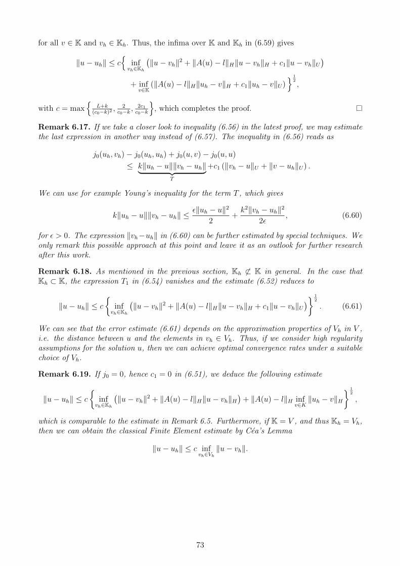
for all v ∈ K and vh ∈ Kh. Thus, the infima over K and Kh in (6.59) gives

∥u− uh∥ ≤ c

infvh∈Kh

(∥u− vh∥2 + ∥A(u)− l∥H∥u− vh∥H + c1∥u− vh∥U

)+ inf

v∈K(∥A(u)− l∥H∥uh − v∥H + c1∥uh − v∥U)

12,

with c = max

L+k(c0−k)2 ,

2c0−k ,

2c1c0−k

, which completes the proof.

Remark 6.17. If we take a closer look to inequality (6.56) in the latest proof, we may estimatethe last expression in another way instead of (6.57). The inequality in (6.56) reads as

j0(uh, vh)− j0(uh, uh) + j0(u, v)− j0(u, u)

≤ k∥uh − u∥∥vh − uh∥⏞ ⏟⏟ ⏞T

+c1 (∥vh − u∥U + ∥v − uh∥U) .

We can use for example Young’s inequality for the term T , which gives

k∥uh − u∥∥vh − uh∥ ≤ ϵ∥uh − u∥2

2+k2∥vh − uh∥2

2ϵ, (6.60)

for ϵ > 0. The expression ∥vh−uh∥ in (6.60) can be further estimated by special techniques. Weonly remark this possible approach at this point and leave it as an outlook for further researchafter this work.

Remark 6.18. As mentioned in the previous section, Kh ⊂ K in general. In the case thatKh ⊂ K, the expression T1 in (6.54) vanishes and the estimate (6.52) reduces to

∥u− uh∥ ≤ c

inf

vh∈Kh

(∥u− vh∥2 + ∥A(u)− l∥H∥u− vh∥H + c1∥u− vh∥U

) 12

. (6.61)

We can see that the error estimate (6.61) depends on the approximation properties of Vh in V ,i.e. the distance between u and the elements in vh ∈ Vh. Thus, if we consider high regularityassumptions for the solution u, then we can achieve optimal convergence rates under a suitablechoice of Vh.

Remark 6.19. If j0 = 0, hence c1 = 0 in (6.51), we deduce the following estimate

∥u− uh∥ ≤ c

inf

vh∈Kh

(∥u− vh∥2 + ∥A(u)− l∥H∥u− vh∥H

)+ ∥A(u)− l∥H inf

v∈K∥uh − v∥H

12

,

which is comparable to the estimate in Remark 6.5. Furthermore, if K = V , and thus Kh = Vh,then we can obtain the classical Finite Element estimate by Cea’s Lemma

∥u− uh∥ ≤ c infvh∈Vh

∥u− vh∥.

73

Chapter 7

Numerical results

The aim of this chapter is to perform numerical tests for the obstacle problem (4.60) thesimplified Signorini problem (4.44) and validate the estimates, which have been presented inExample 6.9 and Example 6.10, respectively. Many effective different methods have beendeveloped to compute Finite Element solutions for variational inequalities. The first section isdedicated to the obstacle problem and we solve its discrete problem in terms of dual problemsfollowing the ideas of [37] and [38] and penalization methods referring to [13, Chapter 1], [18,Chapter 4] and [19, Chapter 4]. We compare the different methods and analyze the errorsof the discrete solutions and the convergence rates. For the simplified Signorini problem, weonly use the penalization technique to compute numerical solutions and compare the resultswith Example 6.10. The last section of this chapter is dedicated to a more realistic frictionproblem, analyzing the displacements of an elastic body in frictional contact with a rigid platefor different friction coefficients. The numerical examples have been performed using the freeFinite Element software FreeFem++, see [36].

7.1 Numerical results for the obstacle problem

Recalling the variational form of the obstacle problem (4.59), we have:Find u ∈ K = v ∈ H1

0 (Ω) | v ≥ ψ in Ω, such that∫Ω

∇u · ∇(v − u) dx ≥∫Ω

f(v − u) dx for all v ∈ K, (7.1)

where f and ψ are sufficiently smooth and ψ ≤ 0 on ∂Ω. The discrete formulation is:Find uh ∈ Kh = vh ∈ Vh | vh(xnode) ≥ ψ(xnode) in every node xnode, such that∫

Ω

∇uh · ∇(vh − uh) dx ≥∫Ω

f(vh − uh) dx for all vh ∈ Kh. (7.2)

We always consider the unit square Ω = [0, 1]× [0, 1] as the computational domain and use a

triangulation Th = T1, T2, . . . , TM of Ω, where Ti = T i are triangular elements andM⋃i

Ti = Ω,

c.f. [4, Chapter 2]. Further, we choose the finite dimensional space Vh ⊂ V as

Vh = vh ∈ C(Ω) | vh|T ∈ P1 for all T ∈ Th and vh = 0 on Γ = ∂Ω, (7.3)

where

P1 = v(x, y) =∑i+j≤1i,j≥0

aijxiyj, aij ∈ R.

74

For the fundamental Finite Element theory we highly recommend [4, Chapter 2] and do notgo further into detail. Since our problem is a variational inequality, we cannot convert thevariational formulation into a linear system directly. Instead, we introduce two different tech-niques, the saddle point problem (dual method) and the penalty method, and formulate thevariational inequality as an equality, where additional terms must be added in order to satisfythe inequality.

7.1.1 Dual methods

We start with a dual method and consider the saddle point problem for the obstacle problem asdescribed in [36]. We do not go into the theory of dual problems, but we just use the algorithmin [36] in order to compare it with the penalty method in the upcoming subsection. For themathematical description and analysis of saddle point problems we refer to [37] and [38]. Thevariational form (7.1) can be rewritten as a saddle point problem: Find u ∈ H1

0 (Ω), λ ∈ L2(Ω)such that

maxλ∈L2(Ω)λ≥0

minu∈H1

0 (Ω)L(u, λ) = 1

2

∫Ω

[∇u · ∇v − fu+ λ(ψ − u)+

]dx, (7.4)

where (ψ − u)+ = max(0, ψ − u). This saddle point problem is equivalent to:Find u ∈ H1

0 (Ω), λ ∈ L2(Ω), such that∫Ω

[∇u · ∇v + λv+

]dx =

∫Ω

fv dx for all v ∈ H10 (Ω),∫

Ω

µ(ψ − u)+ dx = 0 for all µ ∈ L2(Ω), µ ≥ 0, λ ≥ 0.

(7.5)

A possible algorithm to solve (7.5) is the following, c.f. [36], [37] and [38].

Algorithm 1: Solve saddle point problem (7.5)

k = 0, kmax = 100, choose λ0 ∈ H−1(Ω), choose penalty parameter c large enough;for k = 0, 1, ..., kmax do

Set Ik = x ∈ Ω | λk + c(ψ − uk+1) ≤ 0 ;Set Vψ,k+1 = v ∈ H1

0 (Ω) | v = ψ on Ik ;Set V0,k+1 = v ∈ H1

0 (Ω) | v = 0 on Ik ;Find uk+1 ∈ Vψ,k+1 and λk+1 ∈ H−1(Ω), such that∫

Ω

∇uk+1 · ∇vk+1 dx =

∫Ω

fvk+1 dx for all vk+1 ∈ V0,k+1,

⟨λk+1, v⟩ =∫Ω

∇uk+1 · ∇v − fv dx for all v ∈ H10 (Ω)

end

We solve the saddle point problem (7.5) with Algorithm 1 for two different values for f andψ.

Example 7.1. Let f = −2 and ψ = (x−x2)(y−y2). First, we compute the reference solution,meaning that we compute the solution via Algorithm 1 on a very fine triangular mesh andchoose higher order polynomials for the shape functions. In our case, Ω is divided into a mesh

75

Figure 7.1: Zoomed computational domain Ω = [0, 1]× [0, 1], which is divided into a triangularmesh with 200× 200 grid points.

with 200× 200 grid points, see Figure 7.1, and we use P2-elements, where

P2 = v(x, y) =∑i+j≤2i,j≥0

aijxiyj, aij ∈ R.

We solve now the variational inequality (7.2) with Algorithm 1 for different meshes sizeshj = (1/2)j, j = 1, ..., 8, and with P1-elements, where these solutions are referred to as discretesolutions uh. The errors of the discrete solutions uh with respect to the reference solution uand the convergence rates can be observed with respect to the H1-norm and L2-norm, as givenin Table 7.1. We compute the numerical convergence rates ri by using the formula

ri =log(ej+1

ej

)log(hj+1

hj

) , j = 1, 2, . . . , 8, (7.6)

where ej = ∥u− uh∥i for mesh size hj and i = 1, 2.

dof h ∥u− uh∥1 r1 ∥u− uh∥0 r09 0.5 0.278838 0.045433325 0.25 0.159107 0.809433 0.0143888 1.6588181 0.125 0.0829626 0.939463 0.00386289 1.89719289 0.0625 0.0420212 0.981344 0.000986677 1.969031089 0.03125 0.0210929 0.994358 0.000248258 1.990744225 0.015625 0.0105597 0.998188 6.21819e-05 1.9972716641 0.0078125 0.0052813 0.999607 1.55539e-05 1.9992266049 0.00390625 0.00264053 1.00006 3.88889e-06 1.99984

Table 7.1: Errors for different mesh sizes h and their convergence rates ri for f = −2 andψ = (x− x2)(y − y2) with respect to H1- norm and L2-norm, respectively.

76

Figure 7.2: Iso-values of the reference solution u for f = −2 and ψ = (x−x2)(y−y2) computedby means of the saddle point problem.

Recalling the error estimate (6.31) of Example 6.9, i.e.

∥u− uh∥1 ≤ ch,

∥u− uh∥0 ≤ ch2,

we observe from Table 7.1, that the dependency on the mesh size h of the error agrees with thecomputed error of the numerical example in the respective norms.

Furthermore, we investigate the iso-values of the reference solution and compare them withthe discrete solutions. Figure 7.2 shows the values of the reference solution u. We can see fromFigure 7.3, that the discrete solution uh converges to u as h → 0. In addition, the iso-valuesof uh agrees with the ones of the reference solution u as h→ 0. We will compare this examplewith itself but computed by a different method, i.e. the penalty method.

Example 7.2. Let f = −x and ψ = −0.5. As in the previous example, we first compute thereference solution u and investigate the dependency on the mesh size h of the error. Table 7.2shows the error and the convergence rates in theH1-norm and L2-norm, respectively. Analyzingthe error and convergence rates in Table 7.2, we observe that the dependency of the mesh sizeh in the error agrees with the a-priori estimates in Example 6.9, i.e. ∥u − uh∥1 ≤ ch and∥u− uh∥0 ≤ ch2. Figure 7.4 shows the iso-values of the reference solution u.

77

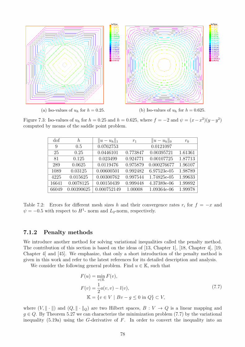
(a) Iso-values of uh for h = 0.25. (b) Iso-values of uh for h = 0.625.

Figure 7.3: Iso-values of uh for h = 0.25 and h = 0.625, where f = −2 and ψ = (x−x2)(y−y2)computed by means of the saddle point problem.

dof h ∥u− uh∥1 r1 ∥u− uh∥0 r09 0.5 0.0762753 0.012109725 0.25 0.0446101 0.773847 0.00395721 1.6136181 0.125 0.023499 0.924771 0.00107725 1.87713289 0.0625 0.0119476 0.975879 0.000276677 1.961071089 0.03125 0.00600501 0.992482 6.97523e-05 1.987894225 0.015625 0.00300762 0.997544 1.74825e-05 1.9963316641 0.0078125 0.00150439 0.999448 4.37389e-06 1.9989266049 0.00390625 0.000752149 1.00008 1.09364e-06 1.99978

Table 7.2: Errors for different mesh sizes h and their convergence rates ri for f = −x andψ = −0.5 with respect to H1- norm and L2-norm, respectively.

7.1.2 Penalty methods

We introduce another method for solving variational inequalities called the penalty method.The contribution of this section is based on the ideas of [13, Chapter 1], [18, Chapter 4], [19,Chapter 4] and [45]. We emphasize, that only a short introduction of the penalty method isgiven in this work and refer to the latest references for its detailed description and analysis.

We consider the following general problem. Find u ∈ K, such that

F (u) = minv∈K

F (v),

F (v) =1

2a(v, v)− l(v),

K = v ∈ V | Bv − g ≤ 0 in Q ⊂ V,

(7.7)

where (V, ∥ · ∥) and (Q, ∥ · ∥Q) are two Hilbert spaces, B : V → Q is a linear mapping andg ∈ Q. By Theorem 5.27 we can characterize the minimization problem (7.7) by the variationalinequality (5.19a) using the G-derivative of F . In order to convert the inequality into an

78

Figure 7.4: Iso-values of the reference solution u for f = −x and ψ = −0.5.

equality we must introduce the penalty term P : V → R, P (v) = 12∥(Bv − g)+∥Q, where

(f)+ = max(0, f). The penalty term is large the constraint of the set K is not satisfied. Thus,we rewrite the minimization problem (7.7) as: Find uκ ∈ V , such that

Fκ(uκ) = minv∈V

Fκ(v),

Fκ(v) = F (v) +1

κP (v),

(7.8)

where κ > 0 and F (v) as in (7.7). In order to apply Theorem 5.27 on (7.8), we suppose thatthe penalization term P is (weakly) lower semi-continuous and G-differentiable. Furthermore,P has only an impact if the constraint of K is not satisfied, i.e.

P (v) ≥ 0, P (v) = 0 if and only if v ∈ K.

With this assumptions on P , we can apply Theorem 5.27, where the G-derivative of the pe-nalization term must be computed. Following the steps of [18, Chapter 3] we obtain, that theminimization problem (7.8) can be characterized by the variational form:Find uκ ∈ V , such that

a(uκ, v) +1

κ[j(Buκ − g)+, Bv] = l(v) for all v ∈ V, (7.9)

where j : Q → Q∗ is the Riesz map, Q∗ is the dual space of Q and [·, ·] : Q∗ × Q → R is theduality paring in Q∗×Q. We choose the finite dimensional subspace Vh ⊂ V as in (7.3). Hence,the discrete formulation of (7.9) reads as: Find uh in Vh, such that

a(uh, vh) +1

κ[j(Buh − g)+, Bvh] = l(vh) for all vh ∈ Vh. (7.10)

We will use the penalty method to solve the same problems as in Example 7.1 and Example7.2.

79

Example 7.3. As in Example 7.1, we set f = −2 and ψ = (x− x2)(y − y2). In this case, theHilbert space Q = V = H1

0 (Ω), B = I and g = ψ. We compute a reference solution u on afine mesh, again 200 × 200 grid, using P2-elements. With the help of the reference solutionswe can compute the error and convergence rates with the solutions for different mesh sizes andP1-elements, see Table 7.3. We discover that the mesh size dependency of the error agreeswith the obtained error estimates of Example 6.9, i.e. ∥u − uh∥1 ≤ ch and ∥u − uh∥0 ≤ ch2.Furthermore, it can be seen that the errors obtained using the penalty methods are very similarto the errors computed by means of the saddle point problems. Hence, both methods give quitethe same result. This result can be also detected by comparing the iso-values of the solutionsin Figure 7.5 and Figure 7.6 with Figure 7.2 and Figure 7.3.

dof h ∥u− uh∥1 r1 ∥u− uh∥0 r09 0.5 0.278836 0.045433325 0.25 0.159111 0.809383 0.0143888 1.6588181 0.125 0.0829578 0.939585 0.00386289 1.89719289 0.0625 0.04202 0.9813 0.000986671 1.969041089 0.03125 0.0210991 0.993894 0.000248262 1.99074225 0.015625 0.0105598 0.9986 6.21993e-05 1.9968916641 0.0078125 0.00527925 1.00018 1.57638e-05 1.9802866049 0.00390625 0.0026413 0.999083 5.54499e-06 1.50736

Table 7.3: Errors for different mesh sizes h and their convergence rates ri with respect to H1-norm and L2-norm, respectively.

Remark 7.4. The convergence rate r0 in the last line with respect to the L2-norm in Table 7.3is 1.50736, which does not agree with the rates above. The reason is, that the error as well as theconvergence rates are computed in terms of the reference solution, which is an approximationof the exact solution as well. Thus, the approximate solution uh may have the same accuracyas the reference solution u, such that the errors and convergence rates give unexpected values.

Example 7.5. Next, we want to investigate the penalty method with the data as in Example7.2, f = −x and ψ = −0.5. The errors and convergence rates can be observed in Table 7.4and agree with the theory in Example 6.9. The error values and convergence rates are quitesimilar to Table 7.2. The iso-values of the reference solution are even equal to Figure 7.4. Asexplained in Remark 7.4, the convergence rate r0 in the last line of Table 7.4 does not give anexpected value due to the accuracy issues.

dof h ∥u− uh∥1 r1 ∥u− uh∥0 r09 0.5 0.0762746 0.012109725 0.25 0.0446117 0.773778 0.0039572 1.6136181 0.125 0.0234975 0.924918 0.00107725 1.87713289 0.0625 0.0119473 0.975818 0.00027669 1.9611089 0.03125 0.00600719 0.991926 6.97688e-05 1.987624225 0.015625 0.00300765 0.998052 1.74899e-05 1.9960616641 0.0078125 0.00150362 1.0002 4.39397e-06 1.9929366049 0.00390625 0.000752668 0.998355 1.55686e-06 1.49688

Table 7.4: Errors for different mesh sizes h and their convergence rates ri with respect to H1-norm and L2-norm, respectively.

80

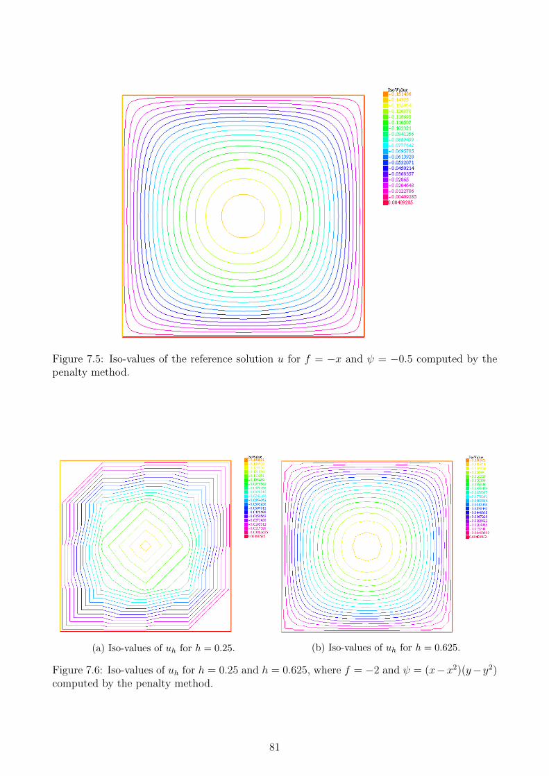
Figure 7.5: Iso-values of the reference solution u for f = −x and ψ = −0.5 computed by thepenalty method.

(a) Iso-values of uh for h = 0.25. (b) Iso-values of uh for h = 0.625.

Figure 7.6: Iso-values of uh for h = 0.25 and h = 0.625, where f = −2 and ψ = (x−x2)(y−y2)computed by the penalty method.

81

7.2 Numerical results for the simplified Signorini prob-

lem

In this section, we turn our attention to the numerical results for the simplified Signoriniproblem (4.25). Recalling the variational form of the simplified Signorini problem (4.27), wehave: Find u ∈ K = v ∈ H1(Ω) | v ≥ 0 on Γ = ∂Ω, such that∫

Ω

∇u · ∇(v − u) + u(v − u) dx ≥∫Ω

f(v − u) dx+

∫Γ

g(v − u) ds for all v ∈ K, (7.11)

where f and g are sufficiently smooth. The discrete formulation is:Find uh ∈ Kh = vh ∈ Vh | vh(xnode) ≥ 0 for every node xnode on the boundary Γ, such that∫Ω

∇uh · ∇(vh − uh) + uh(vh − uh) dx ≥∫Ω

f(vh − uh) dx+

∫Γ

g(vh − uh) ds for all vh ∈ Kh.

(7.12)

We solve the simplified Signorini problem only with the help of the penalty method. For ourexample, we choose f = −2x2 − 2y2 + x2y2 − xy and g = 0. This time, the Hilbert space Q in(7.7) denotes the space L2(Γ). The computational domain is the unit square Ω = [0, 1]× [0, 1].As a slight simplification, we fixed two boundary sides of the domain, i.e. u = 0, and computedthe reference solution on a 250 × 250 grid using P2-elements. Solving the discrete problem(7.12) with the penalty method for different mesh sizes h and with P1-elements, we can observein Table 7.5 the errors and convergence rates with respect to the reference solution u.

dof h ∥u− uh∥1 r1 ∥u− uh∥0 r09 0.5 0.216582 0.021047325 0.25 0.123927 0.805414 0.00525725 2.0012681 0.125 0.0663637 0.90103 0.00139896 1.90995289 0.0625 0.0341887 0.956877 0.000364405 1.940741089 0.03125 0.0172744 0.984879 0.000102346 1.832094225 0.015625 0.00866511 0.995348 5.91655e-05 0.79062816641 0.0078125 0.00434309 0.996497 5.76312e-05 0.037906566049 0.00390625 0.00218799 0.989117 5.81437e-05 -0.0127735

Table 7.5: Errors for different mesh sizes h and their convergence rates ri for f = −2x2−2y2+x2y2 − xy and g = 0 with respect to H1- norm and L2-norm, respectively.

From Table 7.5 it can be deduced that the dependency on the mesh size h of the error agreeswith the a-priori estimates of Example 6.10, i.e. ∥u − uh∥1 ≤ ch and ∥u − uh∥0 ≤ ch2. Theerror and convergence rates with respect to the L2-norm in the last three lines of Table 7.5 donot give expected values due to the accuracy issue as explained in Remark 7.4. Lastly, we plotthe reference solution u in Figure 7.8 and the discrete solutions uh for different mesh sizes hin Figure 7.7. It can be observed that the discrete solution converges to the reference solutionand that the iso-values are very close to each other.

82

(a) Iso-values of uh for h = 0.25. (b) Iso-values of uh for h = 0.625.

Figure 7.7: Iso-values of uh for h = 0.25 and h = 0.625, where f = −2x2 − 2y2 + x2y2 − xy andg = 0 computed by the penalty method.

Figure 7.8: Iso-values of the reference solution u for f = −2x2 − 2y2 + x2y2 − xy and g = 0computed by the penalty method.

7.3 A more realistic example

The aim of this section is to use the mathematical model (5.70) for frictional contact, or rather,its variational formulation (5.76), to consider the contact of a more realistic three-dimensionalproblem. We investigate the contact between an elastic body Ω and a rigid medium F (rigidplate). The elastic body Ω has a cube shape with edge side length A equal to A = 2 · 10−4

and is centered at the origin of the axes. The rigid plate F has the shape of a parallelepiped

83

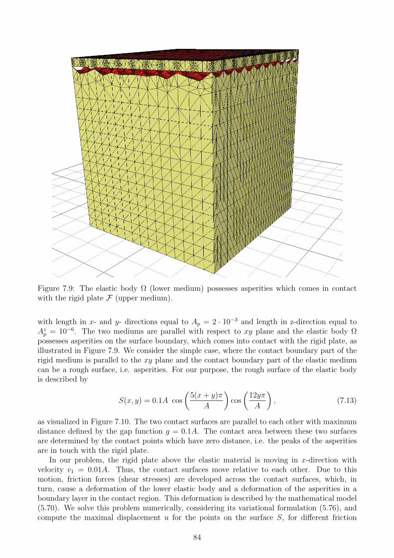
Figure 7.9: The elastic body Ω (lower medium) possesses asperities which comes in contactwith the rigid plate F (upper medium).

with length in x- and y- directions equal to Ap = 2 · 10−3 and length in z-direction equal toAzp = 10−6. The two mediums are parallel with respect to xy plane and the elastic body Ωpossesses asperities on the surface boundary, which comes into contact with the rigid plate, asillustrated in Figure 7.9. We consider the simple case, where the contact boundary part of therigid medium is parallel to the xy plane and the contact boundary part of the elastic mediumcan be a rough surface, i.e. asperities. For our purpose, the rough surface of the elastic bodyis described by

S(x, y) = 0.1A cos

(5(x+ y)π

A

)cos

(12yπ

A

), (7.13)

as visualized in Figure 7.10. The two contact surfaces are parallel to each other with maximumdistance defined by the gap function g = 0.1A. The contact area between these two surfacesare determined by the contact points which have zero distance, i.e. the peaks of the asperitiesare in touch with the rigid plate.

In our problem, the rigid plate above the elastic material is moving in x-direction withvelocity v1 = 0.01A. Thus, the contact surfaces move relative to each other. Due to thismotion, friction forces (shear stresses) are developed across the contact surfaces, which, inturn, cause a deformation of the lower elastic body and a deformation of the asperities in aboundary layer in the contact region. This deformation is described by the mathematical model(5.70). We solve this problem numerically, considering its variational formulation (5.76), andcompute the maximal displacement u for the points on the surface S, for different friction

84

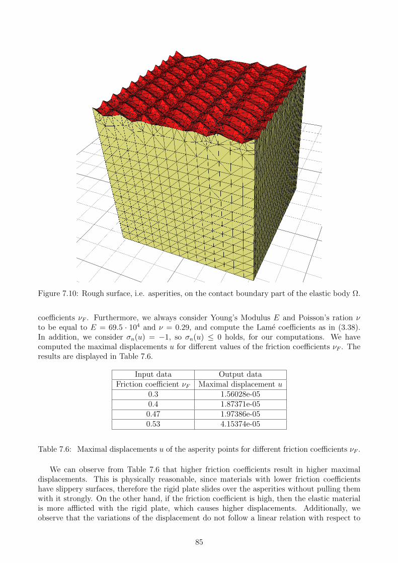
Figure 7.10: Rough surface, i.e. asperities, on the contact boundary part of the elastic body Ω.

coefficients νF . Furthermore, we always consider Young’s Modulus E and Poisson’s ration νto be equal to E = 69.5 · 104 and ν = 0.29, and compute the Lame coefficients as in (3.38).In addition, we consider σn(u) = −1, so σn(u) ≤ 0 holds, for our computations. We havecomputed the maximal displacements u for different values of the friction coefficients νF . Theresults are displayed in Table 7.6.

Input data Output dataFriction coefficient νF Maximal displacement u

0.3 1.56028e-050.4 1.87371e-050.47 1.97386e-050.53 4.15374e-05

Table 7.6: Maximal displacements u of the asperity points for different friction coefficients νF .

We can observe from Table 7.6 that higher friction coefficients result in higher maximaldisplacements. This is physically reasonable, since materials with lower friction coefficientshave slippery surfaces, therefore the rigid plate slides over the asperities without pulling themwith it strongly. On the other hand, if the friction coefficient is high, then the elastic materialis more afflicted with the rigid plate, which causes higher displacements. Additionally, weobserve that the variations of the displacement do not follow a linear relation with respect to

85

the variations of the friction coefficients. In Figure 7.11 we can see the initial configuration ofthe elastic body Ω and its deformed configuration after the movement of the rigid plate.

Figure 7.11: The elastic body Ω deforms relative to the movement of the rigid plate for νF = 0.3.Both, the original and deformed shape of Ω are illustrated for comparison.

86

Chapter 8

Conclusion and Outlook

8.1 Conclusion

In this thesis, we focused on the analysis of abstract elliptic variational and hemi-variationalinequalities. The motivation was the classical Signorini problem (4.25), where we derivedits variational formulation (4.27). We saw that the contact conditions led to restrictions inthe mathematical model, which turned out to be in the form of inequalities and defining thesolution on an admissible set. Furthermore, we obtained a generalized form of variationalinequalities (5.35). We successfully answered the question about the existence of a uniquesolution under strong assumptions as strong monotonicity for the operator A and convexityand lower semi-continuity for the functional j, see Theorem 5.38. Additionally, we providedan analysis of variational inequalities derived from minimization problems, c.f. Theorem 5.31.The variational formulation (5.35) can be associated with frictionless or simplified frictionalcontact problems. However, in order to provide frictional contact problems, hemi-variationalinequalities are essential. They are characterized by the dependence of the functional j on thesolution. We introduced elliptic hemi-variational inequalities (5.47) and answered the questionabout a unique solution as well, see Theorem 5.57. For this purpose, we considered a strongassumption imposed on the functional j, which was (5.49). We examined an application ofhemi-variational inequalities (5.70), where we discovered that frictional problems are by far nosimply solvable problems and that under very strong assumptions on the data a solution canfound. In many works, c.f. [6], [16] and [18], this problem has been investigated and they faceda lot of difficulties.

In addition, we considered the Finite Element discretization of elliptic variational and hemi-variational inequalities. For both cases, we obtained the convergence of the discrete solutionto the exact solution, c.f. Theorem 6.1 and Theorem 6.14, and derived discretization errorestimates in Theorem 6.4 and Theorem 6.16. Unfortunately, solving the variational inequalitynumerically is associated with lots of computational difficulties. Hence, the elaborated conver-gence theory is hard to verify. Recent works of [34], [35], [41] and [45] address this problem andintroduce different methods for solving variational inequalities efficiently.

Lastly, we considered simplified contact problems, i.e. the obstacle problem (7.1) and thesimplified Signorini problem (7.11). We verified the error dependency on the mesh size h derivedin Example 6.9 and Example 6.10 for each problem. We introduced two different numericalmethods, i.e. the dual method by means of saddle point problems and the penalty method. Weobserved similar results for the error behavior solving the obstacle problem with these methods.The last numerical example was dedicated to a more realistic frictional contact problem, wherewe investigated the connection between the displacement and friction coefficient using themathematical model for the Signorini problem with Coulomb friction (5.70).

87

8.2 Outlook

Considering this thesis, there are many possibilities for future work and research. Firstly, wealways considered the contact between an elastic body and a rigid medium. In the litera-ture, this type of contact is usually called unilateral contact. If both bodies are elastic, thenthe deformation of both bodies must be considered and the contact condition becomes morecomplicated. However, this type of contact problem can be also characterized by variationalinequalities.

The analysis of variational inequalities presented in this work has been done for real-valuedHilbert spaces. It is possible to extend this analysis to vector-valued spaces, in order to de-scribe realistic three-dimensional contact problems. However, as we have already remarked,the numerical treatment of more-dimensional contact problems involves a lot of mathematicaldifficulties for complicated contact conditions such as friction. In general, frictional contactproblems are of special interest and many researchers focus on the numerical simulation ofthese type of contact problems. Numerical methods for solving hemi-variational inequalitiesrequire deep mathematical investigation. The computation of an appropriate solution for non-simplified contact problems is still an open research field.

Another possible outlook is to extend the analysis of this work for another types of contact.In terms of tribology, not only firctional contact is of special importance, but also lubrication orwear are essential in engineering applications. Similar mathematical models can be introducedand it is possible to find analogies to this thesis.

In this work, we did not go into detail about Finite Element solvers for variational inequal-ities. We used well known methods as the penalty method or the dual method by means ofthe saddle point problem, for solving the variational inequalities. A direct continuation to thiswork would be the investigation of different Finite Element solvers and an approach to combineparallelization or adaptive methods with the Finite Element method.

Furthermore, the examination of variational inequalities can be enlarged by considering timedependent contact problems, i.e. hyperbolic variational inequalities. Time-dependent problemsdo not only complicate the mathematical model, but also involve more numerical difficultiescompared to elliptic variational inequalities.

Finally, due to the actual research about Artificial Intelligence (AI), there are several ap-proaches to combine the Finite Element methods with AI systems. A possible experimentwould be to go into this direction and solve variational inequalities by Finite Element methodsin terms of AI systems. However, this requires the correct connection between the mathematicalfoundation and the AI systems.

88

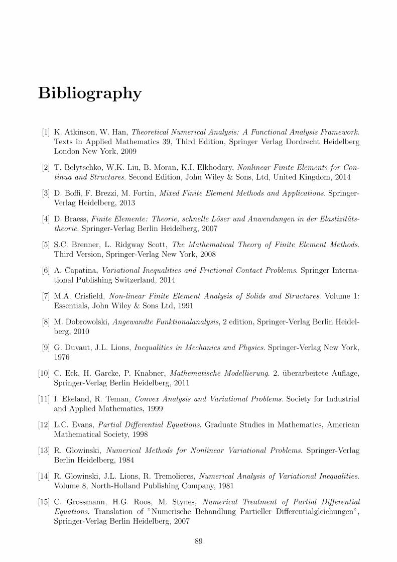
Bibliography

[1] K. Atkinson, W. Han, Theoretical Numerical Analysis: A Functional Analysis Framework.Texts in Applied Mathematics 39, Third Edition, Springer Verlag Dordrecht HeidelbergLondon New York, 2009

[2] T. Belytschko, W.K. Liu, B. Moran, K.I. Elkhodary, Nonlinear Finite Elements for Con-tinua and Structures. Second Edition, John Wiley & Sons, Ltd, United Kingdom, 2014

[3] D. Boffi, F. Brezzi, M. Fortin, Mixed Finite Element Methods and Applications. Springer-Verlag Heidelberg, 2013

[4] D. Braess, Finite Elemente: Theorie, schnelle Loser und Anwendungen in der Elastizitats-theorie. Springer-Verlag Berlin Heidelberg, 2007

[5] S.C. Brenner, L. Ridgway Scott, The Mathematical Theory of Finite Element Methods.Third Version, Springer-Verlag New York, 2008

[6] A. Capatina, Variational Inequalities and Frictional Contact Problems. Springer Interna-tional Publishing Switzerland, 2014

[7] M.A. Crisfield, Non-linear Finite Element Analysis of Solids and Structures. Volume 1:Essentials, John Wiley & Sons Ltd, 1991

[8] M. Dobrowolski, Angewandte Funktionalanalysis, 2 edition, Springer-Verlag Berlin Heidel-berg, 2010

[9] G. Duvaut, J.L. Lions, Inequalities in Mechanics and Physics. Springer-Verlag New York,1976

[10] C. Eck, H. Garcke, P. Knabner, Mathematische Modellierung. 2. uberarbeitete Auflage,Springer-Verlag Berlin Heidelberg, 2011

[11] I. Ekeland, R. Teman, Convex Analysis and Variational Problems. Society for Industrialand Applied Mathematics, 1999

[12] L.C. Evans, Partial Differential Equations. Graduate Studies in Mathematics, AmericanMathematical Society, 1998

[13] R. Glowinski, Numerical Methods for Nonlinear Variational Problems. Springer-VerlagBerlin Heidelberg, 1984

[14] R. Glowinski, J.L. Lions, R. Tremolieres, Numerical Analysis of Variational Inequalities.Volume 8, North-Holland Publishing Company, 1981

[15] C. Grossmann, H.G. Roos, M. Stynes, Numerical Treatment of Partial DifferentialEquations. Translation of ”Numerische Behandlung Partieller Differentialgleichungen”,Springer-Verlag Berlin Heidelberg, 2007

89

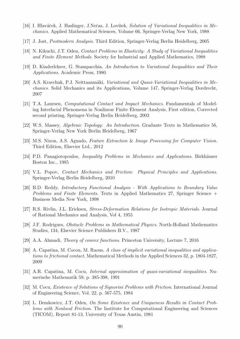
[16] I. Hlavacek, J. Haslinger, J.Necas, J. Lovısek, Solution of Variational Inequalities in Me-chanics. Applied Mathematical Sciences, Volume 66, Springer-Verlag New York, 1988

[17] J. Jost, Postmodern Analysis. Third Edition, Springer-Verlag Berlin Heidelberg, 2005

[18] N. Kikuchi, J.T. Oden, Contact Problems in Elasticity: A Study of Variational Inequalitiesand Finite Element Methods. Society for Industrial and Applied Mathematics, 1988

[19] D. Kinderlehrer, G. Stampacchia, An Introduction to Variational Inequalities and TheirApplications. Academic Press, 1980.

[20] A.S. Kravchuk, P.J. Neittaanmaki, Variational and Quasi-Variational Inequalities in Me-chanics. Solid Mechanics and its Applications, Volume 147, Springer-Verlag Dordrecht,2007

[21] T.A. Laursen, Computational Contact and Impact Mechanics. Fundamentals of Model-ing Interfacial Phenomena in Nonlinear Finite Element Analysis, First edition, Correctedsecond printing, Springer-Verlag Berlin Heidelberg, 2003

[22] W.S. Massey, Algebraic Topology: An Introduction. Graduate Texts in Mathematics 56,Springer-Verlag New York Berlin Heidelberg, 1967

[23] M.S. Nixon, A.S. Aguado, Feature Extraction & Image Processing for Computer Vision.Third Edition, Elsevier Ltd., 2012

[24] P.D. Panagiotopoulos, Inequality Problems in Mechanics and Applications. BirkhauserBoston Inc., 1985

[25] V.L. Popov, Contact Mechanics and Friction: Physical Principles and Applications.Springer-Verlag Berlin Heidelberg, 2010

[26] B.D. Reddy, Introductory Functional Analysis - With Applications to Boundary ValueProblems and Finite Elements. Texts in Applied Mathematics 27, Springer Science +Business Media New York, 1998

[27] R.S. Rivlin, J.L. Ericksen, Stress-Deformation Relations for Isotropic Materials. Journalof Rational Mechanics and Analysis, Vol 4, 1955

[28] J.F. Rodrigues, Obstacle Problems in Mathematical Physics. North-Holland MathematicsStudies, 134, Elsevier Science Publishers B.V., 1987

[29] A.A. Ahmadi, Theory of convex functions. Princeton University, Lecture 7, 2016

[30] A. Capatina, M. Cocou, M. Raous, A class of implicit variational inequalities and applica-tions to frictional contact. Mathematical Methods in the Applied Sciences 32, p. 1804-1827,2009

[31] A.R. Capatina, M. Cocu, Internal approximation of quasi-variational inequalities. Nu-merische Mathematik 59, p. 385-398, 1991

[32] M. Cocu, Existence of Solutions of Signorini Problems with Friction. International Journalof Engineering Science, Vol. 22, p. 567-575, 1984

[33] L. Demkowicz, J.T. Oden, On Some Existence and Uniqueness Results in Contact Prob-lems with Nonlocal Friction. The Institute for Computational Engineering and Sciences(TICOM), Report 81-13, University of Texas Austin, 1981

90

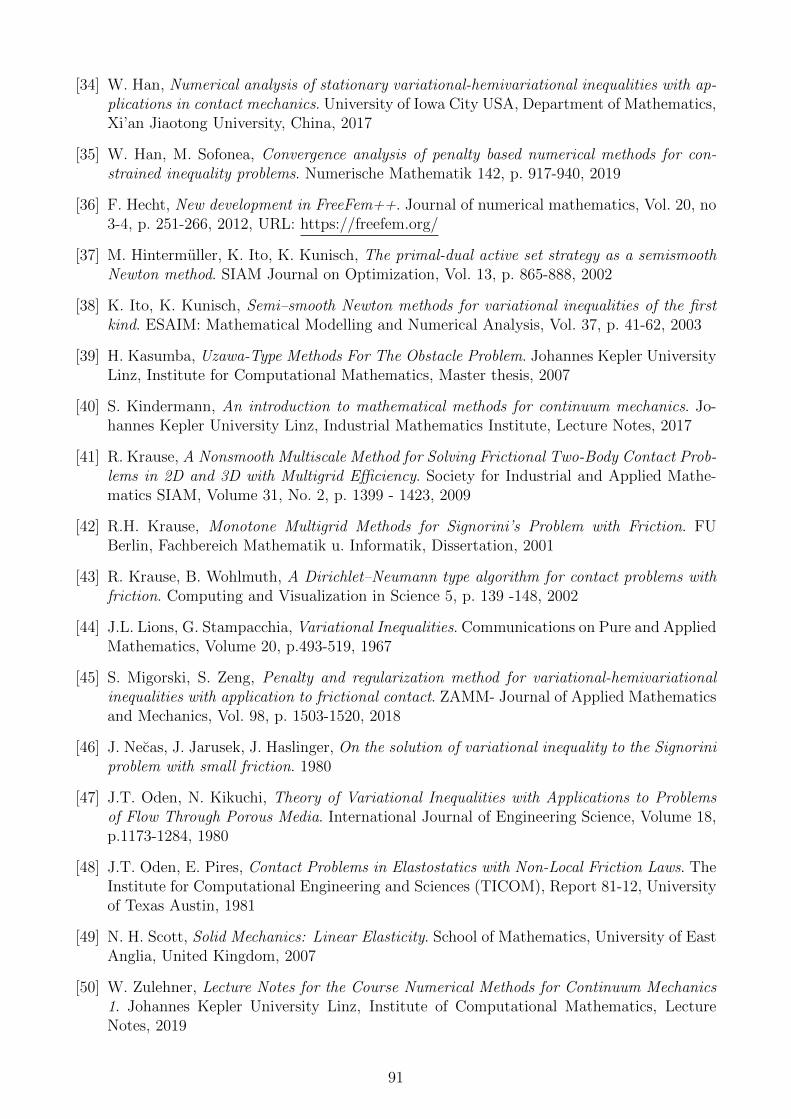
[34] W. Han, Numerical analysis of stationary variational-hemivariational inequalities with ap-plications in contact mechanics. University of Iowa City USA, Department of Mathematics,Xi’an Jiaotong University, China, 2017

[35] W. Han, M. Sofonea, Convergence analysis of penalty based numerical methods for con-strained inequality problems. Numerische Mathematik 142, p. 917-940, 2019

[36] F. Hecht, New development in FreeFem++. Journal of numerical mathematics, Vol. 20, no3-4, p. 251-266, 2012, URL: https://freefem.org/

[37] M. Hintermuller, K. Ito, K. Kunisch, The primal-dual active set strategy as a semismoothNewton method. SIAM Journal on Optimization, Vol. 13, p. 865-888, 2002

[38] K. Ito, K. Kunisch, Semi–smooth Newton methods for variational inequalities of the firstkind. ESAIM: Mathematical Modelling and Numerical Analysis, Vol. 37, p. 41-62, 2003

[39] H. Kasumba, Uzawa-Type Methods For The Obstacle Problem. Johannes Kepler UniversityLinz, Institute for Computational Mathematics, Master thesis, 2007

[40] S. Kindermann, An introduction to mathematical methods for continuum mechanics. Jo-hannes Kepler University Linz, Industrial Mathematics Institute, Lecture Notes, 2017

[41] R. Krause, A Nonsmooth Multiscale Method for Solving Frictional Two-Body Contact Prob-lems in 2D and 3D with Multigrid Efficiency. Society for Industrial and Applied Mathe-matics SIAM, Volume 31, No. 2, p. 1399 - 1423, 2009

[42] R.H. Krause, Monotone Multigrid Methods for Signorini’s Problem with Friction. FUBerlin, Fachbereich Mathematik u. Informatik, Dissertation, 2001

[43] R. Krause, B. Wohlmuth, A Dirichlet–Neumann type algorithm for contact problems withfriction. Computing and Visualization in Science 5, p. 139 -148, 2002

[44] J.L. Lions, G. Stampacchia, Variational Inequalities. Communications on Pure and AppliedMathematics, Volume 20, p.493-519, 1967

[45] S. Migorski, S. Zeng, Penalty and regularization method for variational-hemivariationalinequalities with application to frictional contact. ZAMM- Journal of Applied Mathematicsand Mechanics, Vol. 98, p. 1503-1520, 2018

[46] J. Necas, J. Jarusek, J. Haslinger, On the solution of variational inequality to the Signoriniproblem with small friction. 1980

[47] J.T. Oden, N. Kikuchi, Theory of Variational Inequalities with Applications to Problemsof Flow Through Porous Media. International Journal of Engineering Science, Volume 18,p.1173-1284, 1980

[48] J.T. Oden, E. Pires, Contact Problems in Elastostatics with Non-Local Friction Laws. TheInstitute for Computational Engineering and Sciences (TICOM), Report 81-12, Universityof Texas Austin, 1981

[49] N. H. Scott, Solid Mechanics: Linear Elasticity. School of Mathematics, University of EastAnglia, United Kingdom, 2007

[50] W. Zulehner, Lecture Notes for the Course Numerical Methods for Continuum Mechanics1. Johannes Kepler University Linz, Institute of Computational Mathematics, LectureNotes, 2019

91