Variaonal)principles)) )) Op%mality)in)nature)
34
Varia%onal principles and Op%mality in nature Andrej Cherkaev Department of Mathema%cs University of Utah [email protected] USAG November 2013.
Transcript of Variaonal)principles)) )) Op%mality)in)nature)

Varia%onal principles and
Op%mality in nature
Andrej Cherkaev Department of Mathema%cs University of Utah
USAG November 2013.

Components of applied math
Op%miza%on
Numerical Methods
Differen%al equa%ons Math
Modeling
Sta%s%cs approx
Applied math
Physics, or biologogy, or chemisty, or ..
Why study applied math? • Applied Math is one of the most pres%gious and favored
profession. Everyone needs applied math.
• The applied math problems are inspired by a nature phenomenon or a social need. The phenomena is modeled and rigorously inves%gated. This work combines social value, elegance and beauty.
• Study of applied problems lead to development of calculus, linear algebra, geometry, probability, etc.
• And, yes, we can also teach. In academia, we work on our own problems and collaborate with our colleagues in departments of science, engineering, mining, finances, and medicine.

Op%mality The desire for op%mality (perfec%on) is inherent for human race. The
search for extremes inspires mountaineers, scien%sts, mathema%cians, and the rest of the human race.
• Dante: All that is superfluous displeases God and Nature All that displeases God and Nature is evil.
In engineering, op%mal projects are considered beau%ful and ra%onal, and the far-‐from-‐op%mal ones are called ugly and meaningless. Obviously, every engineer tries to create the best project and he/she relies on op%miza%on methods to achieve the goal.
Two types of op%miza%on problems: 1. Find an op%mal solu%on (engineering) 2. Understand op%mality of a natural phenomenon (science)

Beginning: Geometry Isoperimetric Problem (Dido Problem)
• Probably the first varia%onal problem (isoperimetric problem) has been solved by wise Dido, founder and queen of Carthage the mighty rival of Rome:
• What is the area of land of maximum area that can be encircled by a rope of given length?
• Four hinges proof by Jacob Steiner
• 1. The domain is convex • 2. In the perimeter is cut in half, the area is cut too. • 3. The hinge argument

Search for op%mality in Nature
• The general principle by Pierre Louis Maupertuis (1698-‐1759) proclaims: If there occur some changes in nature, the amount of ac;on necessary for this change must be as small as possible. This principle proclaims that the nature always finds the "best" way to reach a goal.”
• Leonhard Euler: "Since the fabric of the Universe is most perfect and is the work of a most wise Creator, nothing whatsoever takes place in the Universe in which some rela%on of maximum and minimum does not appear."
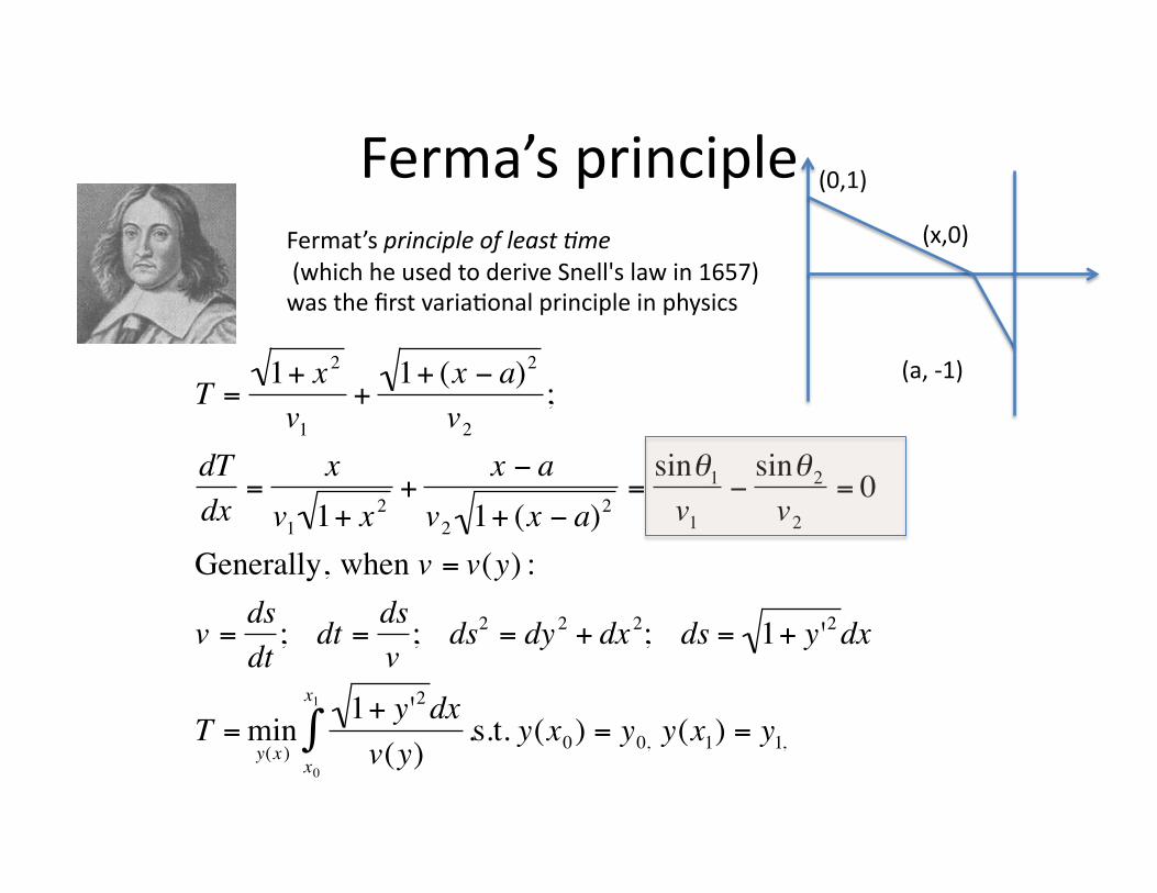
Ferma’s principle
€
T =1+ x 2
v1+
1+ (x − a)2
v2;
dTdx
=x
v1 1+ x 2+
x − av2 1+ (x − a)2
=sinθ1
v1−
sinθ2
v2= 0
Generally, when v = v(y) :
v =dsdt
; dt =dsv
; ds2 = dy 2 + dx 2; ds = 1+ y '2dx
T = miny(x )
1+ y'2dxv(y)
.s.t. y(x0) = y0,x0
x1
∫ y(x1) = y1,
Fermat’s principle of least ;me (which he used to derive Snell's law in 1657) was the first varia%onal principle in physics
(0,1)
(a, -‐1)
(x,0)

Brachistochrone
• Johann Bernulli challenge: (June 1696): Find the shape of the curve down which a bead sliding from rest and accelerated by gravity will slip (without fric<on) from one point to another in the least <me.
• … it is known with certainty that there is scarcely anything which more greatly excites noble and ingenious spirits to labors which lead to the increase of knowledge than to propose difficult and at the same ;me useful problems through the solu;on of which, as by no other means, they may aCain to fame and build for themselves eternal monuments among posterity.
• Five solu%ons were obtained by: Johann Bernulli himself, Leibniz, L'Hospital, Newton, and Jacob Bernoulli.

Brachistochrone
• Brachistochrone is the same Fermat problem, but the speed is defined from the conserva%on of energy law:
€
12mv 2 = mgy⇒ v = 2gy
T = miny(x )
1+ y'2dxv(y)x0
x1
∫ = miny(x )
1+ y '2dx2gyx0
x1
∫
s.t. y(x0) = y0,,y(x1) = y1,
€
x = C(θ − sinθ) +C1,y = C(1− cosθ )
Solu%on: an inverted cycloid
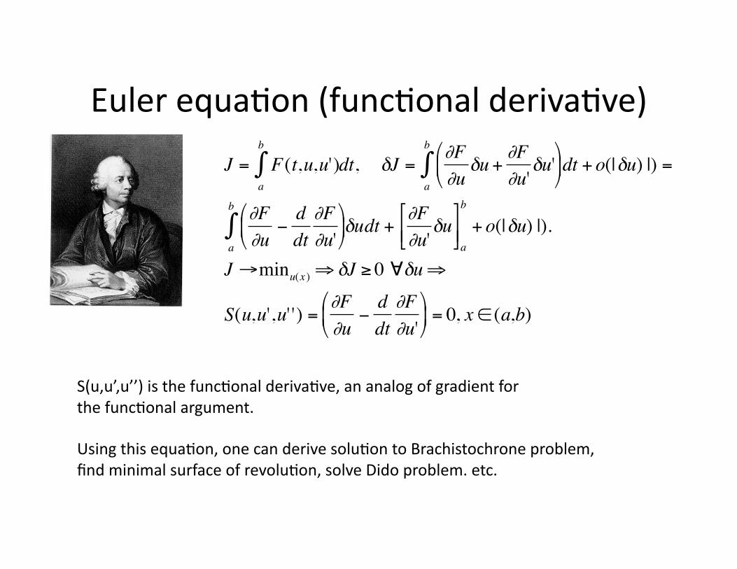
Euler equa%on (func%onal deriva%ve)
€
J = F(t,u,u')a
b
∫ dt, δJ =∂F∂u
δu+∂F∂u'
δu'⎛
⎝ ⎜
⎞
⎠ ⎟ dt
a
b
∫ + o(|δu) |) =
∂F∂u
−ddt∂F∂u'
⎛
⎝ ⎜
⎞
⎠ ⎟ δudt +
a
b
∫ ∂F∂u'
δu⎡
⎣ ⎢ ⎤
⎦ ⎥ a
b
+ o(|δu) |).
J →minu(x ) ⇒δJ ≥ 0 ∀δu⇒
S(u,u',u' ') =∂F∂u
−ddt∂F∂u'
⎛
⎝ ⎜
⎞
⎠ ⎟ = 0, x ∈ (a,b)
S(u,u’,u’’) is the func%onal deriva%ve, an analog of gradient for the func%onal argument.
Using this equa%on, one can derive solu%on to Brachistochrone problem, find minimal surface of revolu%on, solve Dido problem. etc.

Lagrangian • Lagrange applied Euler equa%on to
reformulate Newton law of mo%on:
€
mu' '= f (*)
δ12a
b
∫ m u'( )2dx⎛
⎝ ⎜
⎞
⎠ ⎟ = (mu' ')δu
δ V (u)a
b
∫ dx⎛
⎝ ⎜
⎞
⎠ ⎟ =V 'δu ( f =V ')
(*)⇒δ (K −V )a
b
∫ dx⎛
⎝ ⎜
⎞
⎠ ⎟ = 0
K =12m u'( )2
Lagrange, Mécanique analy%que
"The admirers of the Analysis will be pleased to learn that Mechanics became one of its new branches”
The reader will find no figures in this work. The methods which I set forth do not require either construc%ons or geometrical or mechanical reasoning: but only algebraic opera%ons, subject to a regular and uniform rule of procedure.
Why minus?

Lagrangian
Is Newton law of mo%on equivalent to minimiza%on of ac%on K-‐V ?
If so, then our world is indeed "the best of all possible worlds" according to Golried Leibniz (1710)
Examples:
€
mu' '+cu = 0⇔δ (K −V∫ )dx = 0
K =12m(u')2, V =
12c(u)2
Oscillator Celes%al mechanics
€
K =12
mi(ρi ')2,
i∑
V =12
Gmim j
| ρi − ρ j |i, j∑
ρi ' '=Gm j
| ρi − ρ j |3
i, j∑ (ρi − ρ j )

Oops! Jacobi varia%on. • The Euler equa%on is the sta%onarity condi%on.
Does it correspond to a local minimum? • Look at second varia%on. Assume that S(u)=0, then
€
δ 2J =∂ 2F∂u2⎡
⎣ ⎢
⎤
⎦ ⎥ (δu)2 +
∂ 2F∂u'2⎡
⎣ ⎢
⎤
⎦ ⎥ (δu')2 +
∂ 2F∂u'∂u
δu'∂u⎛
⎝ ⎜
⎞
⎠ ⎟ dt
a
b
∫ + o(|δu)2 |)
J →minu(x ) ⇒δJ = 0, δ 2J ≥ 0 ∀δuExample
€
K =12m(u')2, V =
12c(u)2
δ 2J = m(δu')2 − c(δu)2( )dt0
b
∫
Take δu = ε t(b − t). δ 2J = εb3c30
b2 −10mc
⎛
⎝ ⎜
⎞
⎠ ⎟ , δ 2J < 0 if b >
10mc
For long trajectories, the second varia%on changes its sign! (Newton law is an instant rela%on_.

Saving the natural minimal principle through
unnatural geometry • In Minkowski geometry, the %me axis is imaginary, the
distance is computed as
• If we replace t = i τ, kine%c energy changes its sign, T-‐> -‐T and ac%on becomes the nega%ve of sum of kine%c and poten%al energies.
• L is s%ll real because the of double differen%a%on. • The sta%onary equa%ons are the same, but the energy in
Minkovsky geometry reaches its maximum.
€
ds2 = dx 2 + dy 2 + dz2 − dt 2
€
ddt
=didτ, K = −
m2
dudτ⎛
⎝ ⎜
⎞
⎠ ⎟ 2
, L = −(K +V )
€
L = −m2
dudτ⎛
⎝ ⎜
⎞
⎠ ⎟ 2
−c2u2 S(u) = m du2
dτ 2⎛
⎝ ⎜
⎞
⎠ ⎟ + cu = 0; −m du2
dt⎛
⎝ ⎜
⎞
⎠ ⎟ + cu = 0
€
δ 2J = − c(δu)2 +m(δu')2( )dta
b
∫ ≤ 0 (max)
Example: An oscillator
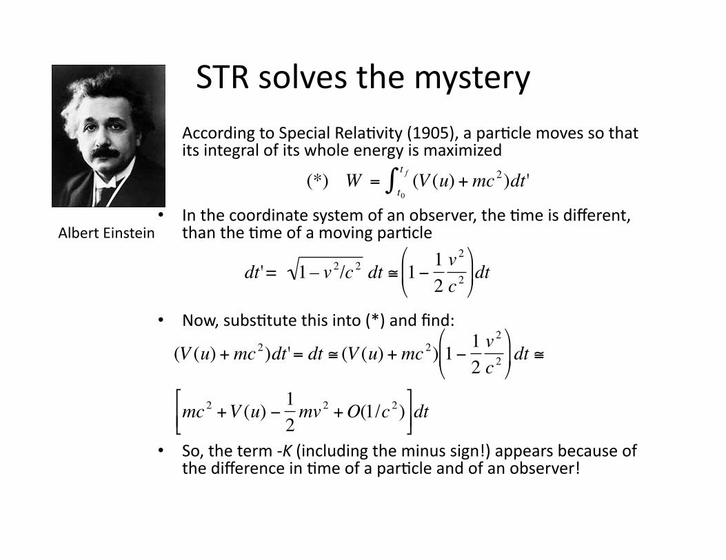
STR solves the mystery • According to Special Rela%vity (1905), a par%cle moves so that
its integral of its whole energy is maximized
• In the coordinate system of an observer, the %me is different, than the %me of a moving par%cle
• Now, subs%tute this into (*) and find:
• So, the term -‐K (including the minus sign!) appears because of the difference in %me of a par%cle and of an observer!
€
(*) W = (V (u) +mc 2t0
t f∫ )dt '
€
dt' = 1– v 2/c 2 dt ≅ 1− 12v 2
c 2
⎛
⎝ ⎜
⎞
⎠ ⎟ dt
€
(V (u) +mc 2)dt'= dt ≅ (V (u) +mc 2) 1− 12v 2
c 2⎛
⎝ ⎜
⎞
⎠ ⎟ dt ≅
mc 2 +V (u) − 12mv 2 +O(1/c 2)
⎡
⎣ ⎢ ⎤
⎦ ⎥ dt
Albert Einstein

Other (contemporary) varia%onal principles in con%nua
A stable equilibrium is always a local minimum of the energy Systems with many equilibria lead to a chao%c mo%on or jerky transi%ons
between them (proteins, crash of a construc%on).
• The principle of maximal energy release rate in cracking • The principle of maximal energy dissipa%on • Minimum entropy principle in chemical reac%ons
• Biological principles: The mathema%cal method: evolu%onary games that model animal or
human behavior models, establishing their evolu%onary usefulness

Op%mality of evolu%on R. A. Fisher's Fundamental theorem of natural selec<on,
in Gene;cal theory of natural selec;on (1930)
The rate of increase in fitness of any organism at any ;me is equal to its gene;c variance in fitness at that ;me. A living being maximizes Inclusive fitness – the probability to send its genes to the next genera%on
Fisher’s example: • Between two groups (male and female) of different sizes s1 and s2, s1 < s2,
the probabili%es p1 and p2 to find a mate from the opposite group are, respec%vely:
The smaller group s1 is in a berer posi%on, therefore, its size increases, and is grows faster. The equilibrium is reached when s1=s2.
• Why the elec;on results are always close? €
p1 =s2
s1 + s2, p2 =
s1s1 + s2
, p1 > p2.
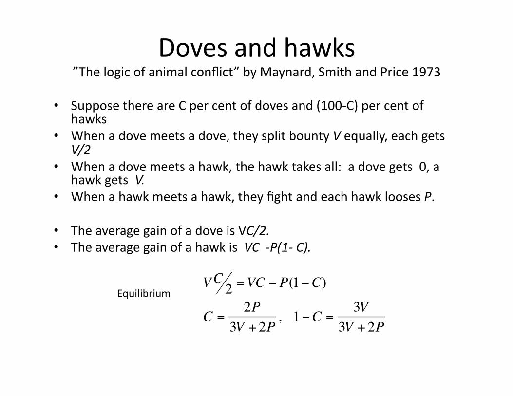
Doves and hawks ”The logic of animal conflict” by Maynard, Smith and Price 1973
• Suppose there are C per cent of doves and (100-‐C) per cent of hawks
• When a dove meets a dove, they split bounty V equally, each gets V/2
• When a dove meets a hawk, the hawk takes all: a dove gets 0, a hawk gets V.
• When a hawk meets a hawk, they fight and each hawk looses P.
• The average gain of a dove is VC/2. • The average gain of a hawk is VC -‐P(1-‐ C).
Equilibrium
€
VC 2 =VC − P(1−C)
C =2P
3V + 2P, 1−C =
3V3V + 2P
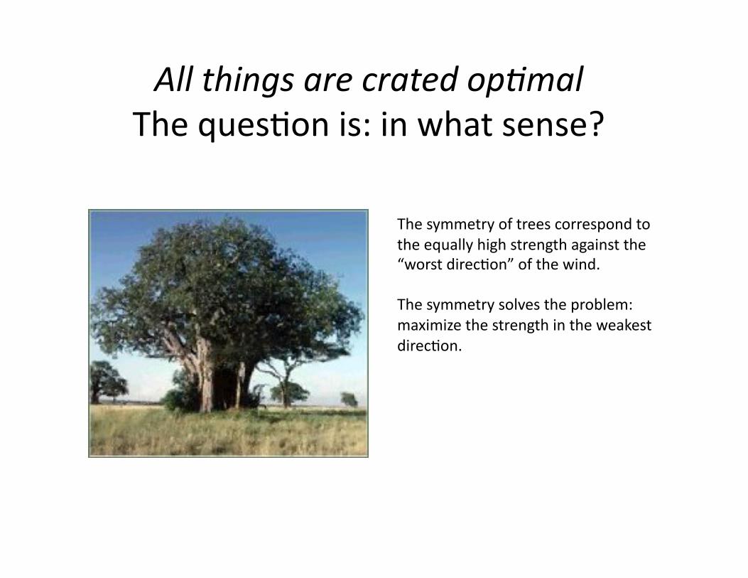
All things are crated op;mal The ques%on is: in what sense?
The symmetry of trees correspond to the equally high strength against the “worst direc%on” of the wind.
The symmetry solves the problem: maximize the strength in the weakest direc%on.

Mistery of spriral trees math.utah.edu/~cherk/spiral-‐trees/story.html
• Why do they spiral? • Postulate: If a natural design becomes
more complex, there is a reason behind. • Problem: find the goal func%onal that
reaches its minimum at realis%c angles (about 45o of spiraling).
• The answer is not unique. Spiraling allow to keep the symmetry when roots at one side die. It is a compromise between the length of the path along the thread from a root to a brunch, and flexibility due to spiraling.
• S. Leelavanishkul and A. Ch. 2004, 2009

Novel branches of varia%onal calculus Problems without solu%ons
• infinitely oscilla%ng minimizing sequence (Laurence Young, 1905-‐2000)
€
J =u(x ):u(0)=0,u(1)=0
inf R(u), R(u) = (u')2 −1( )2+ u2[ ]
0
1
∫ dx
R(u) ≥ 0∀u; find a minimizing sequence u s : limJ( u s) = 0.
1. | u s ' |=1⇒ R( u s) = us2[ ]
0
1
∫ dx
2. u s(x) =x, if x ∈ 0, 1
2s[ )1
2s − x, if x ∈ 12s, 1
s[ )⎧
⎨ ⎪
⎩ ⎪ , u s(x) is 1
s - periodic
u(x) u’(x)

Mul%dimensional problem: Op%mal composite
Problem: Find materials’ layout that minimizes the energy of the system (the work of applied forces) plus the total cost of materials.
Feature: Infinite fast alterna%ons, the faster the berer. This %me, the solu%on also depends on geometrical shape of mixing the subdomains of pure materials, because of boundary condi%ons: normal stress and tangent deforma%on stay con%nuous at the boundary between several materials:
Maximal s%ffness Minimal s%ffness
€
Ceff = m1C1 +m2C2
€
Ceff =m1C1
+m2
C2
⎛
⎝ ⎜
⎞
⎠ ⎟
−1

Two-‐material op%mal structures adapt to an anisotropy of a loading
Hydrosta%c stresss
Unidirec%onal stress Pure shear
Color code: orange – strong material blue -‐-‐ weak material, white -‐-‐ void.
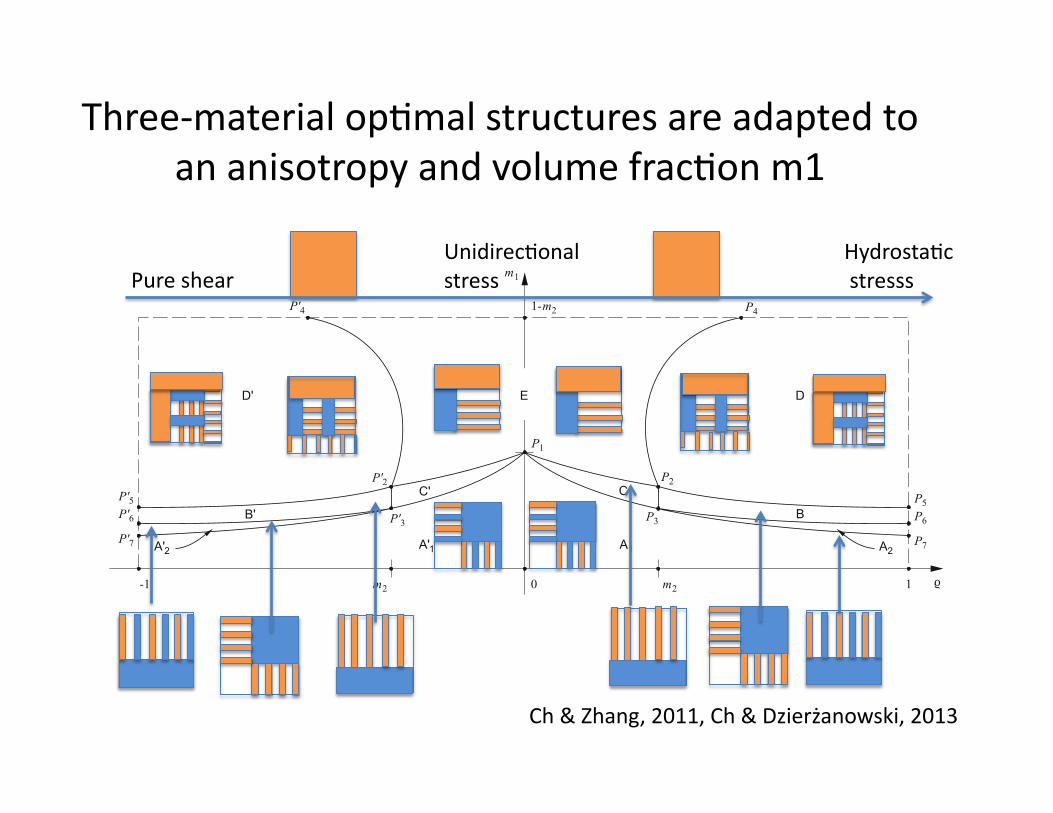
Three-‐material op%mal structures are adapted to an anisotropy and volume frac%on m1
Hydrosta%c stresss
Unidirec%onal stress Pure shear
Ch & Zhang, 2011, Ch & Dzierżanowski, 2013

Op%mal geometries are not unique. Isotropic wheel assemblages
Hashin-‐Shtrikman type assembly
Elements, in dependence on volume frac<on of the best (white field) material.
A.Cherkaev, 2011 strong – white, intermediate – gray, void – black.

Lower cost g2: structures
A{er the first transi%on, P1 always enters the 1-‐2-‐3 structures (gray areas) via 1-‐3 laminate.
No%ce that the op%mal structures for more intensive fields correspond to P1-‐P2 composites.

Special case of the materials’ cost
The graph shows the op%mal structures in dependence of eigenvalues of the external stress field. Large stresses correspond to the op%mality of pure s%ff material. Gray fields show three–material structures.
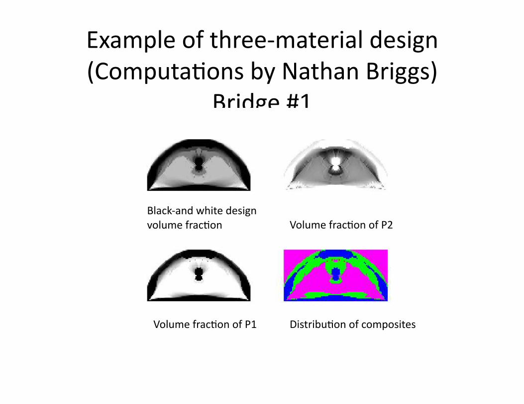
Example of three-‐material design (Computa%ons by Nathan Briggs)
Bridge #1
Black-‐and white design volume frac%on
Volume frac%on of P1
Volume frac%on of P2
Distribu%on of composites

Bridge #2, smaller total weight

Can%lever, loaded at the middle

Can%lever, loaded at the the edge

Thank you!

A{er physics, op%mality of evolu%on • Instead of ac%on, a living being maximizes Inclusive fitness –
the probability to send its genes to the next genera%on. Selfish Gene by Richard Dawkins 1976.
• The mathema%cal method: evolu%onary games. • Example: • Between two groups (male and female) of different sizes s1 and
s2, s1 < s2, the probabili%es p1 and p2 to find a mate from the opposite group are:
• The smaller group is in a berer posi%on and its size increases, so is grows faster. The equilibrium is reached when s1=s2.
• • Why the elec;on results are always close? €
p1 =s2
s1 + s2, p2 =
s1s1 + s2
, p1 > p2.

Plan • Introduc%on: Extremal principles: Descrip%on through minimiza%on. Dido
problem. • History
– Fermat principle. – Calculus of varia%ons. Euler equa%on, Brachistochrone – Lagrange approch – Jacobi Columbus principle. – Special rela%vity. Minkowski geometry.
• Today: – Ra%onality of the evolu%on. – Male and Female newborns. Evolu%onary games – Op%mality of the spiral tree
• Problems without solu%on. – Minimal surface – much ado about nothing.