Studies in Business and Economics no. 14(1)/2019

- 208 -

DOI 10.2478/sbe-2019-0016 SBE no. 14(1) 2019

VARIANTS OF THE TRAVELING SALESMAN PROBLEM

PATTERSON Mike Dillard College of Business, Midwestern State University, USA

FRIESEN Daniel

University of North Texas, Dallas Campus, USA Abstract:

This paper includes an introduction to the concept of spreadsheet optimization and modeling as it specifically applies to combinatorial problems. One of the best known of the classic combinatorial problems is the “Traveling Salesman Problem” (TSP). The classic Traveling Salesman Problem has the objective of minimizing some value, usually distance, while defining a sequence of locations where each is visited once. An additional requirement is that the tour ends in the same location where the tour started. Variants of the classic Traveling Salesman Problem are developed including the Bottleneck TSP and the Variation Bottleneck TSP.

Key words: Optimization, Spreadsheet, Traveling Salesman, Combinatorial

1. Introduction

This paper includes a general introduction to the concept of spreadsheet

optimization and modeling as it specifically applies to combinatorial problems. One of the best known of the classic combinatorial problems is the “Traveling Salesman Problem” (TSP). In the definitive The Traveling Salesman Problem: A Guided Tour of Combinatorial Optimization (1985) Lawler et. al. introduce the Traveling Salesman Problem (TSP) as “a salesman, starting from his home city, is to visit exactly once each city on a given list and then return home, it is plausible for him to select the order in which he visits the cities so that the total of the distances traveled in his tour is as small as possible”. Cummings (June 2000) traces the roots of the problem to Karl Menger, who defined the problem, which he referred to as the “Messenger Problem” published “Das botenproblem” in Ergenbnisse eines Mathematischen Kolloquiums in 1932. In tracing the historical roots of the TSP Lawler et. al. (1985) credit Merrill Flood as being responsible for publicizing the conceptual basis for the TSP in the operations community. Robinson’s paper “On the Hamiltonian Game” (1949) is frequently cited as a seminal work. Lawler et. al. (1985) cite “Solution of a large-scale traveling-salesman problem by Dantzig, Fulkerson and Johnson (1954) as a

Studies in Business and Economics no. 14(1)/2019

- 209 -

critical event in the development of the TSP and combinatorial optimization in general. Dantzig, one of the giants in operations research, is frequently referred to as the “Father of Linear Programming” (Albers and Reid, 1986). Among the more popular combinatorial problems which have been subject to optimization include permutations, sequencing and scheduling, the minimal spanning tree, and the traveling salesman problem. Tuza (2001) provides a particularly comprehensive set of challenging and unsolved combinatorial problems.

2. General Model Description

The classic Traveling Salesman Problem has the objective of minimizing some

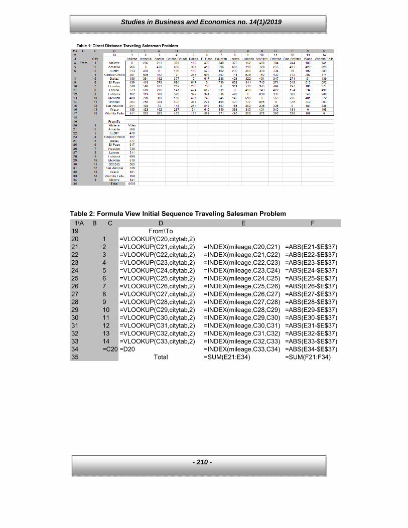
value, usually distance, while defining a sequence of locations where each is visited once. An additional requirement is that the tour ends in the same location where the tour started. The spreadsheet model utilized in this paper is patterned after a model developed by Patterson and Harmel (2003). The initial base problem is defined in Table 1, cells D4:R14. There are fourteen locations to be visited on the tour. The upper portion of Table 1 displays the direct distance between each of the locations. The lower portion of the spreadsheet (Cells D20:E34) display the distance between the cities when they are in the initial (i.e. alphabetical/random) sequence. The sum of the initial tour distance (5508) is also displayed.

Excel Solver was utilized as the software for development of this model. Solver is an add-in software tool in Excel for modeling general purpose linear and non-linear optimization problems. It was developed by Frontline Systems. Solver provides an option known as the “alldifferent” constraint, which is particularly useful in combinatorial problems, such as the traveling salesman problem. (Frontline Systems, n.d.)

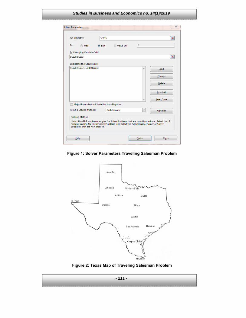
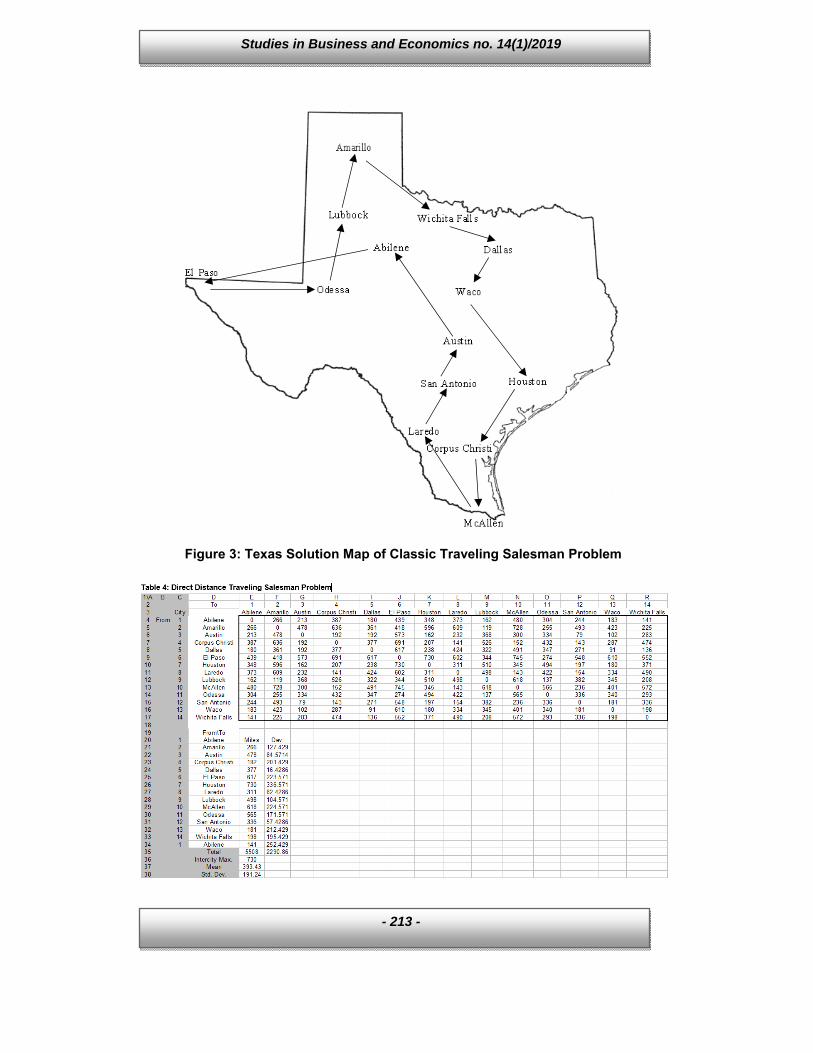
Table 2 displays the lower portion of the spreadsheet with the formula view. Figure 1 displays the Solver parameters for the classical traveling salesman problem. The objective is to minimize the total distance traveled. The constraints include that each city must be visited once and that the tour must end in the same city which it began. The alldifferent constraint efficiently defines these constraints. The standard evolutionary engine is required in order to utilize the alldifferent option required to satisfy the constraints. Figure 2 displays a visual of the problem. Table 3 displays the Solver solution to the classic Traveling Salesman Problem. The visual solution is shown in Figure 3. As indicated the total distance traveled for the suggested trip is 2,549 miles.

Studies in Business and Economics no. 14(1)/2019

- 210 -

Table 2: Formula View Initial Sequence Traveling Salesman Problem

1\A B C D E F19 From\To20 1 =VLOOKUP(C20,citytab,2)21 2 =VLOOKUP(C21,citytab,2) =INDEX(mileage,C20,C21) =ABS(E21-$E$37)22 3 =VLOOKUP(C22,citytab,2) =INDEX(mileage,C21,C22) =ABS(E22-$E$37)23 4 =VLOOKUP(C23,citytab,2) =INDEX(mileage,C22,C23) =ABS(E23-$E$37)24 5 =VLOOKUP(C24,citytab,2) =INDEX(mileage,C23,C24) =ABS(E24-$E$37)25 6 =VLOOKUP(C25,citytab,2) =INDEX(mileage,C24,C25) =ABS(E25-$E$37)26 7 =VLOOKUP(C26,citytab,2) =INDEX(mileage,C25,C26) =ABS(E26-$E$37)27 8 =VLOOKUP(C27,citytab,2) =INDEX(mileage,C26,C27) =ABS(E27-$E$37)28 9 =VLOOKUP(C28,citytab,2) =INDEX(mileage,C27,C28) =ABS(E28-$E$37)29 10 =VLOOKUP(C29,citytab,2) =INDEX(mileage,C28,C29) =ABS(E29-$E$37)30 11 =VLOOKUP(C30,citytab,2) =INDEX(mileage,C29,C30) =ABS(E30-$E$37)31 12 =VLOOKUP(C31,citytab,2) =INDEX(mileage,C30,C31) =ABS(E31-$E$37)32 13 =VLOOKUP(C32,citytab,2) =INDEX(mileage,C31,C32) =ABS(E32-$E$37)33 14 =VLOOKUP(C33,citytab,2) =INDEX(mileage,C32,C33) =ABS(E33-$E$37)34 =C20 =D20 =INDEX(mileage,C33,C34) =ABS(E34-$E$37)35 Total =SUM(E21:E34) =SUM(F21:F34)

Studies in Business and Economics no. 14(1)/2019

- 211 -

Figure 1: Solver Parameters Traveling Salesman Problem

Figure 2: Texas Map of Traveling Salesman Problem

Studies in Business and Economics no. 14(1)/2019

- 212 -

As stated previously, the primary purpose of this study is to present two alternative models to the TSP. The first variation to the classic Traveling Salesman Problem is the Bottleneck Traveling Salesman Problem (BTSP). Conceptually, the BTSP is quite similar to the TSP. The constraints are identical in that each location must be visited once. In other words, each location must be entered once and exited once. Also, the trip must end in the same city where it began. The only real formulation difference is that rather than minimizing the total distance of the trip, the objective is to minimize the distance of the single longest intercity trip (Lawler, et. al., 1985). With this one change to the objective function, the classic TSP is converted to a “minimax” problem where the objective is to minimize the maximum single distance between two cities. The second alteration to the TSP is to modify the objective function to minimize the degree of variation around the mean intercity trip difference. In other words, to the extent it is possible, we desire to make each intercity trip as close as possible to the mean distance. Once again the constraints are identical to the TSP. The difference is in the statement of the objective function. In our formulation we chose to minimize the standard deviation of the distances for the selected tour sequence. Table 4 displays the complete initial spreadsheet for the all three new models. Additional statistical calculations displayed include the intercity maximum value, the mean intercity distance and the standard deviation for the intercity distances. Table 5 displays the formula view for relevant cells. In addition, column F displays the deviation from the mean for each intercity trip.

Table 3: Solution to Traveling Salesman Problem

1\A B C D E19 From\To20 1 Abilene Miles21 3 Austin 21322 12 San Antonio 7923 8 Laredo 15424 10 McAllen 14325 4 Corpus Christi 15226 7 Houston 20727 13 Waco 18028 5 Dallas 9129 14 Wichita Falls 13630 2 Amarillo 22531 9 Lubbock 11932 11 Odessa 13733 6 El Paso 27434 1 Abilene 43935 Total 2549

Studies in Business and Economics no. 14(1)/2019

- 213 -

Figure 3: Texas Solution Map of Classic Traveling Salesman Problem

Studies in Business and Economics no. 14(1)/2019

- 214 -

Table 5: Formula View Initial Sequence Three Traveling Salesman Problem 1\A B C D E F

19 From\To20 1 =VLOOKUP(C20,citytab,2)21 2 =VLOOKUP(C21,citytab,2) =INDEX(mileage,C20,C21) =ABS(E21-$E$37)22 3 =VLOOKUP(C22,citytab,2) =INDEX(mileage,C21,C22) =ABS(E22-$E$37)23 4 =VLOOKUP(C23,citytab,2) =INDEX(mileage,C22,C23) =ABS(E23-$E$37)24 5 =VLOOKUP(C24,citytab,2) =INDEX(mileage,C23,C24) =ABS(E24-$E$37)25 6 =VLOOKUP(C25,citytab,2) =INDEX(mileage,C24,C25) =ABS(E25-$E$37)26 7 =VLOOKUP(C26,citytab,2) =INDEX(mileage,C25,C26) =ABS(E26-$E$37)27 8 =VLOOKUP(C27,citytab,2) =INDEX(mileage,C26,C27) =ABS(E27-$E$37)28 9 =VLOOKUP(C28,citytab,2) =INDEX(mileage,C27,C28) =ABS(E28-$E$37)29 10 =VLOOKUP(C29,citytab,2) =INDEX(mileage,C28,C29) =ABS(E29-$E$37)30 11 =VLOOKUP(C30,citytab,2) =INDEX(mileage,C29,C30) =ABS(E30-$E$37)31 12 =VLOOKUP(C31,citytab,2) =INDEX(mileage,C30,C31) =ABS(E31-$E$37)32 13 =VLOOKUP(C32,citytab,2) =INDEX(mileage,C31,C32) =ABS(E32-$E$37)33 14 =VLOOKUP(C33,citytab,2) =INDEX(mileage,C32,C33) =ABS(E33-$E$37)34 =C20 =D20 =INDEX(mileage,C33,C34) =ABS(E34-$E$37)35 Total =SUM(E21:E34) =SUM(F21:F34)36 Intercity Max. =MAX(E21:E34)37 Mean =AVERAGE(E21:E34)38 Std. Dev. =STDEV(E21:E34)

Figure 4: Solver Parameters Bottleneck Traveling Salesman Problem

Studies in Business and Economics no. 14(1)/2019

- 215 -

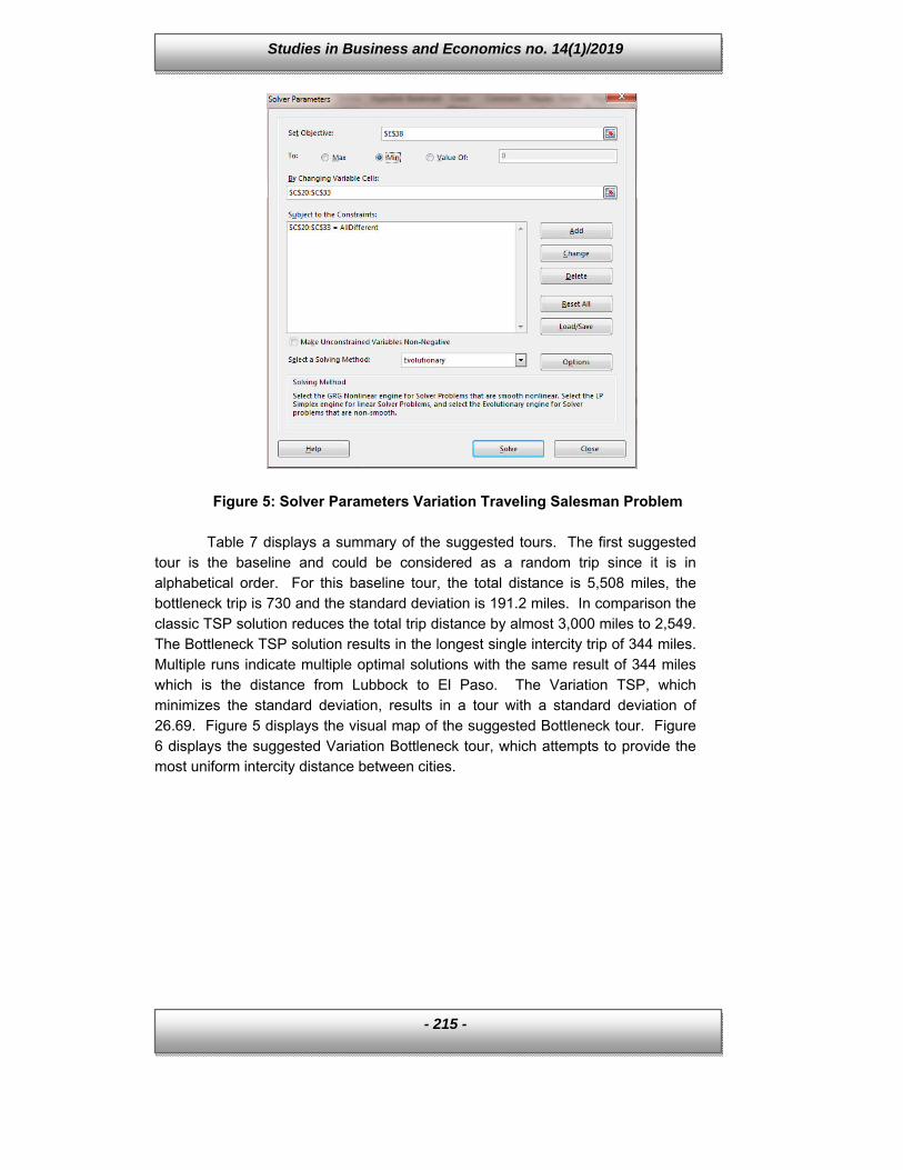
Figure 5: Solver Parameters Variation Traveling Salesman Problem

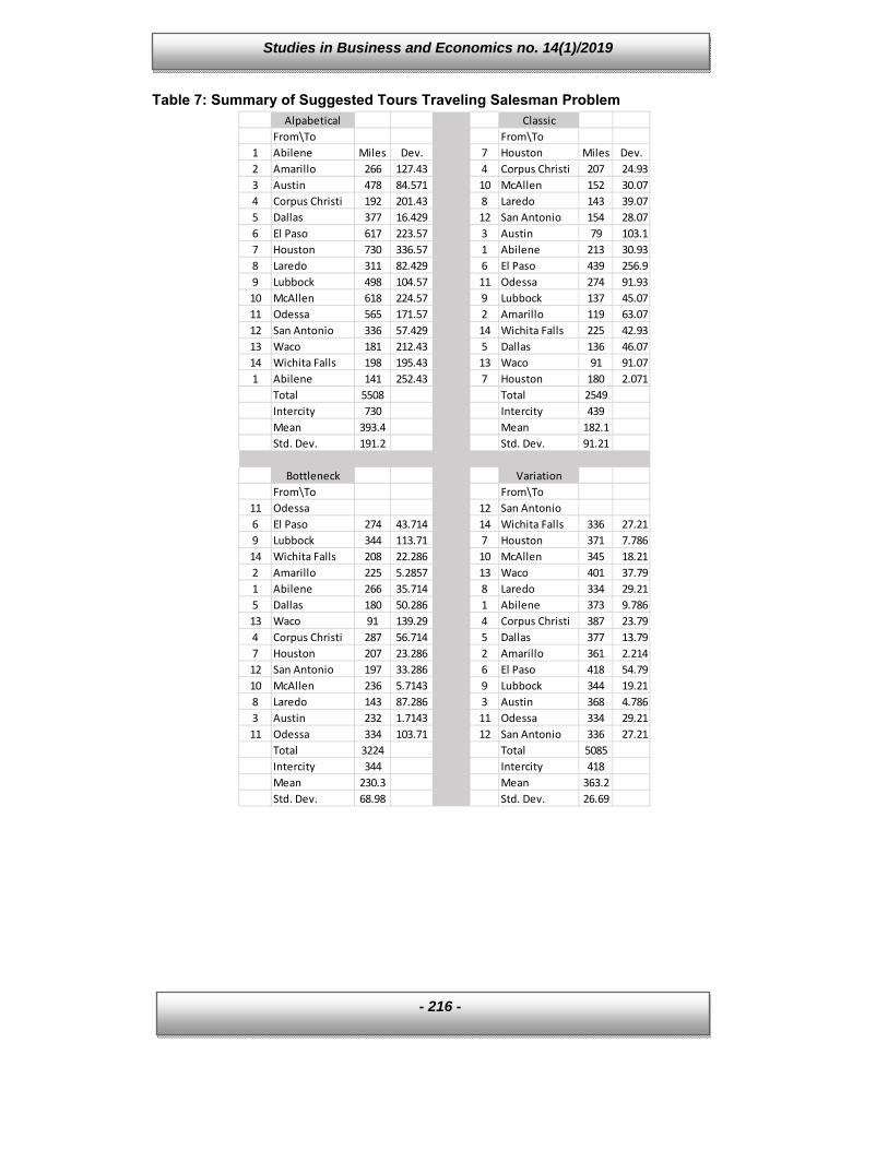
Table 7 displays a summary of the suggested tours. The first suggested tour is the baseline and could be considered as a random trip since it is in alphabetical order. For this baseline tour, the total distance is 5,508 miles, the bottleneck trip is 730 and the standard deviation is 191.2 miles. In comparison the classic TSP solution reduces the total trip distance by almost 3,000 miles to 2,549. The Bottleneck TSP solution results in the longest single intercity trip of 344 miles. Multiple runs indicate multiple optimal solutions with the same result of 344 miles which is the distance from Lubbock to El Paso. The Variation TSP, which minimizes the standard deviation, results in a tour with a standard deviation of 26.69. Figure 5 displays the visual map of the suggested Bottleneck tour. Figure 6 displays the suggested Variation Bottleneck tour, which attempts to provide the most uniform intercity distance between cities.

Studies in Business and Economics no. 14(1)/2019

- 216 -

Table 7: Summary of Suggested Tours Traveling Salesman Problem Alpabetical Classic

From\To From\To

1 Abilene Miles Dev. 7 Houston Miles Dev.

2 Amarillo 266 127.43 4 Corpus Christi 207 24.93

3 Austin 478 84.571 10 McAllen 152 30.07

4 Corpus Christi 192 201.43 8 Laredo 143 39.07

5 Dallas 377 16.429 12 San Antonio 154 28.07

6 El Paso 617 223.57 3 Austin 79 103.1

7 Houston 730 336.57 1 Abilene 213 30.93

8 Laredo 311 82.429 6 El Paso 439 256.9

9 Lubbock 498 104.57 11 Odessa 274 91.93

10 McAllen 618 224.57 9 Lubbock 137 45.07

11 Odessa 565 171.57 2 Amarillo 119 63.07

12 San Antonio 336 57.429 14 Wichita Falls 225 42.93

13 Waco 181 212.43 5 Dallas 136 46.07

14 Wichita Falls 198 195.43 13 Waco 91 91.07

1 Abilene 141 252.43 7 Houston 180 2.071

Total 5508 Total 2549

Intercity 730 Intercity 439

Mean 393.4 Mean 182.1

Std. Dev. 191.2 Std. Dev. 91.21

Bottleneck Variation

From\To From\To

11 Odessa 12 San Antonio

6 El Paso 274 43.714 14 Wichita Falls 336 27.21

9 Lubbock 344 113.71 7 Houston 371 7.786

14 Wichita Falls 208 22.286 10 McAllen 345 18.21

2 Amarillo 225 5.2857 13 Waco 401 37.79

1 Abilene 266 35.714 8 Laredo 334 29.21

5 Dallas 180 50.286 1 Abilene 373 9.786

13 Waco 91 139.29 4 Corpus Christi 387 23.79

4 Corpus Christi 287 56.714 5 Dallas 377 13.79

7 Houston 207 23.286 2 Amarillo 361 2.214

12 San Antonio 197 33.286 6 El Paso 418 54.79

10 McAllen 236 5.7143 9 Lubbock 344 19.21

8 Laredo 143 87.286 3 Austin 368 4.786

3 Austin 232 1.7143 11 Odessa 334 29.21

11 Odessa 334 103.71 12 San Antonio 336 27.21

Total 3224 Total 5085

Intercity 344 Intercity 418

Mean 230.3 Mean 363.2

Std. Dev. 68.98 Std. Dev. 26.69

Studies in Business and Economics no. 14(1)/2019

- 217 -

Figure 5: Texas Solution Map of Bottleneck Traveling Salesman Problem

Figure 6: Texas Solution Map of Variation Traveling Salesman Problem

Studies in Business and Economics no. 14(1)/2019

- 218 -

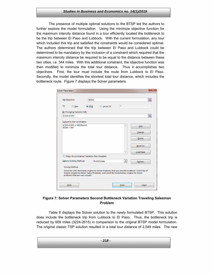
The presence of multiple optimal solutions to the BTSP led the authors to further explore the model formulation. Using the minimize objective function for the maximum intercity distance found in a tour efficiently located the bottleneck to be the trip between El Paso and Lubbock. With the current formulation, any tour which included this trip and satisfied the constraints would be considered optimal. The authors determined that the trip between El Paso and Lubbock could be determined to be mandatory by the inclusion of a constraint which required that the maximum intercity distance be required to be equal to the distance between these two cities, i.e. 344 miles. With this additional constraint, the objective function was then modified to minimize the total tour distance. Thus it accomplishes two objectives. First, the tour must include the route from Lubbock to El Paso. Secondly, the model identifies the shortest total tour distance, which includes the bottleneck route. Figure 7 displays the Solver parameters.

Figure 7: Solver Parameters Second Bottleneck Variation Traveling Salesman Problem

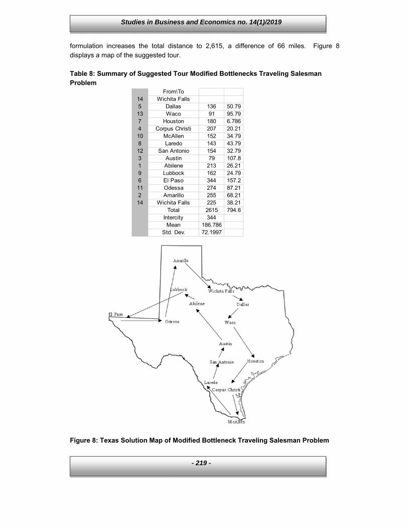
Table 8 displays the Solver solution to the newly formulated BTSP. This solution

does include the bottleneck trip from Lubbock to El Paso. Thus, the bottleneck trip is reduced by 609 miles (3224-2615) in comparison to the original BTSP model formulation. The original classic TSP solution resulted in a total tour distance of 2,549 miles. The new

Studies in Business and Economics no. 14(1)/2019

- 219 -

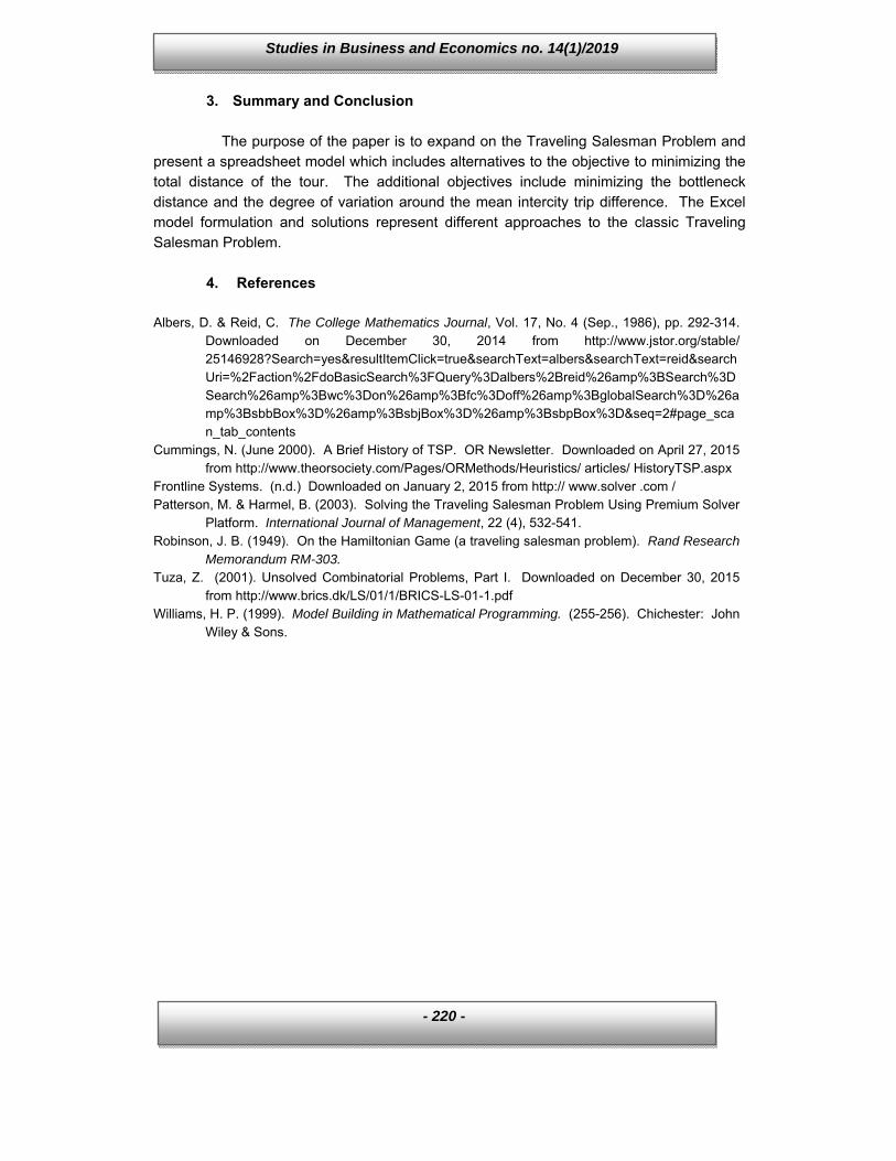
formulation increases the total distance to 2,615, a difference of 66 miles. Figure 8 displays a map of the suggested tour. Table 8: Summary of Suggested Tour Modified Bottlenecks Traveling Salesman Problem

From\To14 Wichita Falls5 Dallas 136 50.7913 Waco 91 95.797 Houston 180 6.7864 Corpus Christi 207 20.2110 McAllen 152 34.798 Laredo 143 43.7912 San Antonio 154 32.793 Austin 79 107.81 Abilene 213 26.219 Lubbock 162 24.796 El Paso 344 157.211 Odessa 274 87.212 Amarillo 255 68.2114 Wichita Falls 225 38.21

Total 2615 794.6Intercity 344Mean 186.786

Std. Dev. 72.1997

Figure 8: Texas Solution Map of Modified Bottleneck Traveling Salesman Problem

Studies in Business and Economics no. 14(1)/2019

- 220 -

3. Summary and Conclusion

The purpose of the paper is to expand on the Traveling Salesman Problem and present a spreadsheet model which includes alternatives to the objective to minimizing the total distance of the tour. The additional objectives include minimizing the bottleneck distance and the degree of variation around the mean intercity trip difference. The Excel model formulation and solutions represent different approaches to the classic Traveling Salesman Problem.

4. References

Albers, D. & Reid, C. The College Mathematics Journal, Vol. 17, No. 4 (Sep., 1986), pp. 292-314.

Downloaded on December 30, 2014 from http://www.jstor.org/stable/ 25146928?Search=yes&resultItemClick=true&searchText=albers&searchText=reid&searchUri=%2Faction%2FdoBasicSearch%3FQuery%3Dalbers%2Breid%26amp%3BSearch%3DSearch%26amp%3Bwc%3Don%26amp%3Bfc%3Doff%26amp%3BglobalSearch%3D%26amp%3BsbbBox%3D%26amp%3BsbjBox%3D%26amp%3BsbpBox%3D&seq=2#page_scan_tab_contents

Cummings, N. (June 2000). A Brief History of TSP. OR Newsletter. Downloaded on April 27, 2015 from http://www.theorsociety.com/Pages/ORMethods/Heuristics/ articles/ HistoryTSP.aspx

Frontline Systems. (n.d.) Downloaded on January 2, 2015 from http:// www.solver .com / Patterson, M. & Harmel, B. (2003). Solving the Traveling Salesman Problem Using Premium Solver

Platform. International Journal of Management, 22 (4), 532-541. Robinson, J. B. (1949). On the Hamiltonian Game (a traveling salesman problem). Rand Research

Memorandum RM-303. Tuza, Z. (2001). Unsolved Combinatorial Problems, Part I. Downloaded on December 30, 2015

from http://www.brics.dk/LS/01/1/BRICS-LS-01-1.pdf Williams, H. P. (1999). Model Building in Mathematical Programming. (255-256). Chichester: John

Wiley & Sons.