Variance Function Regressions for Studying Inequality

CitationWestern, Bruce and Deirdre Bloome. 2009. Variance function regressions for studying inequality. Working paper, Department of Sociology, Harvard University.

Permanent linkhttp://nrs.harvard.edu/urn-3:HUL.InstRepos:2645469

Terms of UseThis article was downloaded from Harvard University’s DASH repository, and is made available under the terms and conditions applicable to Open Access Policy Articles, as set forth at http://nrs.harvard.edu/urn-3:HUL.InstRepos:dash.current.terms-of-use#OAP

Share Your StoryThe Harvard community has made this article openly available.Please share how this access benefits you. Submit a story .

Accessibility

Variance Function Regressions for Studying Inequality

Bruce Western1 Deirdre Bloome

Harvard University

January 2009

1Department of Sociology, 33 Kirkland Street, Cambridge MA 02138. E-mail:western@wjh.harvard.edu. This research was supported by a grant from theRussell Sage Foundation.

Abstract

Regression-based studies of inequality model only between-group differ-ences, yet often these differences are far exceeded by residual inequality.Residual inequality is usually attributed to measurement error or the in-fluence of unobserved characteristics. We present a regression that in-cludes covariates for both the mean and variance of a dependent variable.In this model, the residual variance is treated as a target for analysis. Inanalyses of inequality, the residual variance might be interpreted as mea-suring risk or insecurity. Variance function regressions are illustrated inan analysis of panel data on earnings among released prisoners in the Na-tional Longitudinal Survey of Youth. We extend themodel to a decomposi-tion analysis, relating the change in inequality to compositional changes inthe population and changes in coefficients for the mean and variance. Thedecomposition is applied to the trend in US earnings inequality amongmale workers, 1970 to 2005.

In studying inequality, we can distinguish differences between groups

from differences within groups. Sociological theory usually motivates hy-

potheses about between-group inequality. For these hypotheses, interest

focuses on differences in group averages. For example, theories of labor

market discrimination predict whites earn more than blacks, and men

earn more than women. Human capital theory explains why college grad-

uates average higher earnings than high school dropouts. Such theories

are often tested with a regression where differences in groups means are

quantified by regression coefficients.

Although theory usually focuses on between-group differences, within-

group variance also contributes to inequality. Within-group inequality

can be measured by the residual variance of a regression. Typically the

residual is viewed as unexplained, and its variation is not treated as sub-

stantively interesting. Although it is often overlooked, residual hetero-

geneity may vary in substantively important ways. Some groups may be

more insecure than others, or vary more in unobserved characteristics.

The structure of within-group inequality may be especially important for

sociological analysis where the residual variance often greatly exceeds the

the between-group variance.

We present a statistical model of inequality that captures the effects

of covariates on within-group and between-group inequality. Called a

variance-function regression, the model features separate equations for

the mean and variance of the dependent variable. Regression coefficients

for the mean and variance can be estimated with specialized calculations,

though we show that they are well-approximated in large samples with

standard software.

Though variance function regression have a long history in economet-

1

rics and statistics (Park 1966; Harvey 1976; Cook and Weisberg 1983), we

use them to make three contributions to the sociological analysis of in-

equality. First, from a substantive viewpoint, a statistical model for the

residual variance challenges sociological theory to explain not just aver-

age differences between groups, but also differences in the heterogeneity

of groups. Large coefficients for the residual variance indicate large dif-

ferences in within-group inequality. Below we motivate interest in these

differences in within-group inequality with theories of economic insecu-

rity.

Second, a few studies have analyzed variation in the residual variance,

but only as a function of macro predictors (like metro areas or occupa-

tions), and only using ad hoc methods for estimation. We follow the statis-

tical literature by writing a likelihood that includes regression coefficients

for the conditional mean and the variance. This approach allows macro

and micro predictors for the residual variation and enables the joint esti-

mation of regression coefficients with smaller mean squared error than ad

hoc approaches. We apply the model in an analysis of panel data to test

the hypothesis that men released from prison experience greater earnings

insecurity (greater variance) in addition to the well-documented decline

in average earnings.

Finally, we apply the model to a standard decomposition of the change

in variance. This extension of the decomposition analysis offers a simple

way of studying the effects of individual independent variables on changes

in inequality. In our approach, changes in inequality may result from:

(1) changes in the distribution of an independent variable, (2) changes

in means across levels of an independent variable, or (3) changes in vari-

ances across levels of an independent variable. We also describe a Bayesian

2

approach to estimation that yields inferences for nonstandard quantities

from the variance decomposition, whose sampling uncertainty is usually

ignored. These methods are illustrated in an analysis of the trend in US

earnings inequality using data from the March Current Population Survey.

Between-Group and Within-Group Inequality in Sociology

In a very general sense, sociologists are pervasively interested in between-

group inequality. Most claims about variability in a population describe

average differences between groups. Of course, not all studies of between-

group difference are framed as analyses of inequality. But where inequal-

ity is the focus, it is generally conceived in between-group terms.

The emphasis on between-group inequality seems clearest in theories

emphasizing categorical inequalities—inequalities between categorically

defined groups (Tilly 1998; Massey 2007). In these accounts, out-groups

receive less because in-groups monopolize resources and restrict access to

opportunities. Average differences in incomes, well-being, and mobility

emerge as a result. The labor market theory of discrimination exemplifies

an account of categorical difference whosemain empirical implications are

for between-group inequality. Research on racial and gender discrimina-

tion thus estimates black-white differences, or female-male differences in

earnings, typically controlling for a large number of confounding factors

(Cancio, Evans, and Maume 1996; Budig and England 2001).

Regression provides a convenient framework for this analysis, where

the regression coefficients describe differences in group means. Of course,

regression also describes between-group differences with continuous pre-

dictors. In this case, groups are defined across the fine gradations of the

continuous variable.

3

Although between-group differences dominate sociological thinking

about inequality, the regression model also includes a term for within-

group differences. Write the regression for observation i,

yi = b0 + b1xi + ei,

with expected value yi = b0 + b1xi . With errors, ei , uncorrelated with the

predictors, xi , inequality in yi , measured by the variance, can be expressed

as the sum of the variance between groups and the variance within groups,

V (yi) = V (yi) + V (ei).

↑ ↑Between Within

Group Group

In a least squares regression, the empirical residuals are uncorrelated with

xi by construction, so the variance of yi mechanically equals the sum of the

residual variance and the variance of predicted values for the yi . The resid-

ual variance, V (ei), may reflect measurement error rather than an underly-

ing social process. Often, however, residuals are viewed as capturing real

but substantively uninteresting variation. For example, Blau and Duncan

(1967, 174) remark that residuals reflect a (thankfully) unpredictable so-

cial world, but the magnitude of residuals is unimportant for understand-

ing inequalities in educational attainment or occupational status. “The

relevant question about the residual,” they write, “is not really its size at

all, but whether the unobserved factors it stands for are properly repre-

sented as being uncorrelated with measured antecedent variables” (Blau

and Duncan 1967, 175). From this perspective, residuals are not intrinsi-

cally interesting, but may be helpful for discovering omitted variables.

4

In contrast to Blau and Duncan (1967), residual variability may be a

substantively important difference between groups. For example, among

children at age 10, boys are over-represented in the top tail of the distri-

bution of measured intelligence, and average slightly higher scores than

girls on intelligence tests. However, the over-representation of boys among

highly intelligent children is due significantly to the greater dispersion of

boy’s scores (Arden and Plomin 2006). Here, the salient difference be-

tween boys and girls is not just the location of their test score distributions,

but the spread of those distributions too. Comparing distributions across

groups helps enrich the account of group differences beyond stylized facts

about the difference of means.

In research on inequality, the substantive significance of the residual

was considered in Jencks’s discussion of the income distribution (Jencks et

al. 1972). For Jencks, the large residual variance in regressions on incomes

results fromworkers’ unmeasured skills and luck. An appealing personal-

ity and athletic talent are offered as examples of unmeasured skills. Luck

might include “chance acquaintances who steer you to one line of work

rather than another, the range of jobs that happen to be available in a

particular community when you are job hunting, . . . and a hundred other

unpredictable accidents” (Jencks et al. 1972, 227). The influence of luck

on income inequality might be reduced through insurance, Jencks argues,

suggesting that luck might also be described as income insecurity.

A similar interpretation of the residual variance is provided in recent

research on US income inequality. The growth of US inequality in the

1980s and 1990s was marked by a steady increase in the residual variance

in regressions of earnings on experience and schooling. Labor economists

argued that growth in within-group inequality reflected rising returns to

5

unobserved skills and compositional changes which multiplied the num-

bers of high-skill workers with highly variable incomes (Katz and Murphy

1992; Lemieux 2006). Others, sociologists and economists, countered that

increasing within-group inequality resulted from workers’ increasing ex-

posure to competitive forces in the labor market (DiNardo, Fortin, and

Lemieux 1996; Massey 2007). Institutions like the minimum wage, labor

unions, and the career ladders of large firms made income more secure

and sheltered wages frommarket forces. As these institutional protections

eroded through the 1970s and 1980s, within-group inequality in earnings

increased. McCall (2000) thus refers to the “deinstitutionalization” of the

American labor market, and Sørensen (2000) points to the elimination of

labor market rents as a source of increasing income insecurity. Consis-

tent perhaps with rising returns to unobserved skills and rising economic

insecurity, increased within-group inequality has also been found to be a

driver of inequality in China during the period of rapid market transition

from the late 1980s to the mid-1990s (Hauser and Xie 2005). Theories of

unobserved skill and labor market deinstitutionalization depart from ac-

counts of between-group inequality by claiming that the residual variance

is larger for some groups than others.

Sociological research on within-group inequality has taken residual

standard deviations and other measures of within-group inequality as de-

pendent variables for regression. McCall’s (2000) study of labor mar-

ket institutionalization took a two-stage approach, first regressing log in-

comes on demographic covariates. The residuals from this first-stage re-

gression were used to form residual standard deviations for metro areas

which were then regressed on metro-level measures of employment and

industry-structure. Sørensen and Sorenson (2007) also took a two-stage

6

approach in their analysis of Danish data. Obtaining residuals from a re-

gression on log wages, they calculated log residual standard deviations

for local areas which were regressed on measures of the competitiveness

of local product markets. In contrast to the small-area analysis, Kim and

Sakamoto (2008) regress Gini indexes of occupational wage inequality on

occupation-level predictors. In all these analyses, within-group inequality

is viewed as the product of macro-level predictors. Thus variables mea-

sured at the level of occupational groups or metro areas, for example,

have been written as predictors of within-group inequality. Estimation

proceeds in two stages where residuals are calculated from a first stage re-

gression, and residual dispersion is regressed on macro predictors in the

second stage.

We next introduce a model that jointly estimates the effects of predic-

tors on between-group and within-group inequality. Jointly fitting within-

group and between-group effects takes us beyond macro-level studies of

within-group inequality in two ways. First, our model allows for the ef-

fects of micro-level and macro-level variables on within-group inequal-

ity. Second, by jointly estimating between-group and within-group coeffi-

cients, inferences about one set of coefficients also incorporate uncertainty

about the other.

Formalizing and Estimating the Model

For observation i (i = 1, . . . ,n) on a dependent variable, yi , the variance

function regression writes the mean, yi , and the variance, σ2i , both as a

7

function of covariates,

yi = x′iβ

logσ2i = z′iλ,

where xi is a K ×1 vector of covariates for the mean, and zi is a J ×1 vectorof covariates (possibly equal to xi) for the variance.1 In this this model,

a coefficient βk has the usual interpretation, describing the average differ-

ence in y associated with a one unit change on an independent variable,

xk. Early proposals viewed the variance coefficients, λ, as a diagnostic for

heteroscedasticity (Cook and Weisberg 1983). In studying inequality, the

λ coefficients are substantively interesting, describing the association of

covariates with within-group inequality. A variance coefficient λj is inter-

preted as the difference in the log variance associated with a unit change in

zj . We are familiar with a single observation, yi having a conditional mean

given observations on independent variables, xi , but the idea of a condi-

tional variance for a single observation may be less intuitive. In this case,

the model describes not where yi will fall on average, but how far yi will

fall from this average value, given zi . From a substantive viewpoint, the

model formalizes the idea that values of xi and zi are associated not just

with high or low values of yi but are also associated with the variability or

unpredictability of yi .

The variance functionmodel clearly relaxes some of the assumptions of

the usual linear regression. Unlike the constant variance linear regression,

the variance function model is heteroscedastic, allowing the residual vari-

ance to depend on covariates. Though the variance function regression is1It is often useful to transform the dependent variable to the log scale yielding a scale

invariant measure of inequality, the variance of log yi . We discuss this in greater detailbelow.

8

relatively general, the model assumes that the mean and variance are lin-

ear functions of covariates. The mean and variance of yi are also assumed

to be independent, conditional on xi and zi . The yi are also assumed to

be independent. Each of these assumptions could be relaxed by allowing

for a more general functional form for the regression relationships, or by

specifying a more complex structure for the covariance matrix of yi . The

linearity of the mean and variance functions could be relaxed by adding

nonlinear terms to the regression or by writing the mean and variance as

nonlinear in the parameters. The independence assumption for yi could

be relaxed by allowing cross-correlation terms in the covariance matrix or

by adding random effects in the mean regression. Correlations between

the mean and variance could be allowed by writing the variance as a func-

tion of yi .

Variance function regressions have a relatively long history in statis-

tics and econometrics and were originally motivated by parametric tests

for heteroscedasticity (Anscombe 1961; Park 1966; Cook and Weisberg

1983). Joint maximum likelihood estimation of the mean and variance co-

efficients was developed in subsequent studies (Harvey 1976; Aitkin 1987;

Verbyla 1993). Though we know of no research with these models in so-

ciology, there are recent applications in the sciences and social sciences

which study the effects of covariates on the variance. Agricultural studies

have recently examined variability in the survival rates of fish popula-

tions, and modelled the variance of crop yields (Minto, Myers, and Blan-

chard 2008; Edwards and Jannink 2006). In the social sciences, economists

have studied predictors of retail prices and political scientists have ana-

lyzed the variance of vote choice in referenda (Lewis 2008; Selb 2008).

In all these studies, the structure heteroscedasticity was of key scientific

9

interest.

Estimation

Several methods have been proposed to estimate the variance function

regression. First, a simple two-stage approach uses standard software to

fit a linear regression, then a generalized linear model to the transformed

residuals (Nelder and Lee 1991). For this method:

1. Estimate β with a linear regression of yi on xi . Save the residuals,

ei = yi − x′iβ, where β is the least squares estimate.

2. Estimate λ with a gamma regression of the squared residuals, e2i , on

zi , using a log link function.

The gamma regression is a type of generalized linear model for positive

right-skewed dependent variables. The regression can be fit with standard

software such as the glm command in Stata or GENMOD in SAS. The point

estimates with this method are consistent, but the standard errors are in-

correct. In particular, the standard errors for the estimates of λ take no

account of the uncertainty in β, and estimates of β are inefficient because

they ignore heteroscedasticity in yi .

Second, maximum likelihood estimates are obtained by iterating the

two stage method (Aitkin 1987). In addition to the assumptions above, if

we assumed that yi is conditionally and independently normal with mean

yi and variance σ2i , the contribution of observation i to the log likelihood

is

L(β,λ;yi) = −12[log(σ2i ) + (yi − yi)2/σ2i ]= −12[z′iλ+ di exp(−z′iλ)],

10

where di is the squared residual, (yi − yi)2. To obtain the maximum likeli-hood estimates:

1. Fit a linear regression of yi on xi , yielding the estimated coefficients,

β, and residuals, ei = yi − x′iβ.

2. Fit a gamma regression with a log link of e2i on zi , yielding current

estimates λ. Save the fitted values, σ2i = exp(z′iλ).

3. Fit a weighted linear regression of yi on xi , with weights, 1/σ2i . Up-

date the residuals, ei , and evaluate the log likelihood.

4. Iterate steps 2 and 3 to convergence, updating β and ei from the

linear regression, and λ and σ2i from the gamma regression.

Like many generalized linear models, the gamma regression is commonly

fit by iteratively weighted least squares. If coefficients from the previous

iteration are used as start values, computation can be speeded by fitting

just one step of the gamma regression (Smyth, Huele, and Verbyla 2001,

164). Like the two-stage estimator, ML estimation can be performed with

standard software for generalized linear models. (A Stata macro is given

in Appendix 1.)

The maximum likelihood estimator may perform poorly in small sam-

ples because variance estimation does not adjust for degrees of freedom

and a biased score vector is used for estimation. A restricted maximum

likelihood (REML) estimator based on the marginal likelihood for λ pro-

duces estimates that are less biased in small samples (Smyth, Huele, and

Verbyla 2001). Unlike the two-stage and ML estimation, REML estima-

tion requires specialized calculations. Smyth (2002) describes an efficient

REML algorithm which has been implemented in R.

11

The variance-function regression can also be placed in a Bayesian frame-

work. Bayesian analysis offers two advantages. First in small samples,

the λ coefficients in the variance equation may be skewed and inference

based on the normal distribution will be inaccurate. Nonnormality in the

posterior distribution will be revealed by simulation from the Bayesian

posterior distribution. Second, some analyses, like the variance decompo-

sition below, will focus not on the model coefficients themselves, but on

nonlinear functions of the coefficients. Output from the Bayesian poste-

rior simulation can be used to construct inferences for these functions of

model parameters.

The Bayesian model combines the normal likelihood for yi with a prior

distribution for the coefficients, β, and a hierarchical prior for the variance

coefficients, λ. For a dependent variable, yi , with predictors xi for the

mean and zi for the variance, the Bayesian model can be written:

yi ∼ N(yi ,σ2i ), where

yi = x′iβ and logσ2i = ziλ

with prior distributions,

β ∼ N(b,V )

λ ∼ N(g,U)

Ujj ∼ Gamma−1(u0,u1)

A noninformative prior sets the prior mean vectors, b and g, all to zero.

The K × K prior covariance matrix, V , is diagonal with large prior vari-ances, say 106. To help ensure the sample data dominates estimation of the

variance coefficients, λ is given a hierarchical prior. The J × J covariancematrix, U, is diagonal and the prior variances follow an inverse Gamma

12

distribution with hyperparameters, u0 = .001 and u1 = .001. (We also ex-

perimented with a nonhierarchical prior on λ though this approach per-

formed poorly in small samples.) The Bayesian model can be estimated

with MCMC software like BUGS. (BUGS code is given in Appendix 2.)

Comparing Estimation Methods

The four estimation methods—two-step, ML, REML and Bayes—vary in

ease of application. The two-step and ML methods can be fit with stan-

dard software, while REML and Bayesian estimation require specialized

calculations. Do the four methods perform comparably?

We performed a Monte Carlo experiment to compare two-stage, ML,

and REML, and Bayesian estimators. This experiment was based on one

covariate, xq, a vector consisting of q replicates of x′ = [1,2, . . . ,10]. The

dependent variable, yi was generated from,

yi ∼N(yi ,σ2i ),

where yi = .1+ .1× xqi , and σ2i = exp(.3+ .3× xqi). We generated yi for q = 5and 50, corresponding to sample sizes n = 50 and 500. The four estimators

were applied to each data set of xqi and yi . Estimates were obtained for

2000 replications at each sample size.

The experimental results are reported in Table 1. With the small sam-

ple, n = 50, biases for all estimators are generally modest. However, for the

intercept of the variance function, λ0, bias of theMLE is larger than for the

other estimators by a factor of 2 to 5. Though we might expect the prior

distribution to influence estimates in small samples, bias in the Bayesian

analysis is similar to that for REML. The advantages of likelihood-based

approaches (including Bayes) can be seen by comparing the sampling vari-

13

Table 1. Results from a Monte Carlo experiment for two-stage, ML, REML, andBayesian estimators of a variance-function regression.

β0 β1 λ0 λ1Bias of point estimates, n = 50Two-stage -.024 .004 -.017 -.009ML -.009 .001 -.100 .003REML -.007 .000 -.045 .000Bayes -.011 -.001 -.042 .006

Sampling variance of point estimates, n = 50Two-stage .538 .030 .202 .005ML .312 .018 .212 .005REML .312 .018 .213 .005Bayes .312 .018 .213 .005

Coverage rate of 95% interval, n = 50Two-stage .986 .914 .918 .926ML .945 .939 .906 .917REML .939 .940 .945 .945Bayes .956 .960 .962 .969

Bias of point estimates, n = 500Two-stage .002 -.001 -.002 -.001ML .001 -.001 -.011 .000REML .001 -.001 -.004 .001Bayes -.001 -.001 -.001 .000

Sampling variance of point estimates, n = 500Two-stage .053 .003 .020 .001ML .029 .002 .020 .001REML .029 .002 .020 .001Bayes .029 .002 .020 .001

Coverage rate of 95% interval, n = 500Two-stage .989 .920 .938 .944ML .950 .944 .938 .942REML .950 .944 .943 .943Bayes .950 .945 .958 .950

Note: For each sample size, n = 50 and n = 500, 2000 Monte Carlo samples weredrawn. BUGS code for the Bayesian estimation is reported in the Appendix.

14

ance of point estimates. The sampling variance of β with the two-stage es-

timator is nearly twice as large as the other methods, unsurprising given

the inefficiency of OLS in the presence of heteroscedasticity. The per-

formance of inferential statistics is measured by how frequently nomi-

nal confidence intervals cover the known regression coefficients. Nominal

confidence intervals for the two-stage andML estimator are often too opti-

mistic in small samples, overstating coverage rates. REML and Bayes yield

uniformly more accurate frequentist inference in small samples. REML

standard errors are slightly optimistic, and Bayesian standard errors are

slightly pessimistic, with nominal intervals being long, given their cover-

age rates.

The performance of all the estimators improves as sample size gets

large. With n = 500, there is very little bias in the point estimates of either

β or λ. As sample sizes increase by a factor of 10, sampling variances de-

crease in similar proportion. The two-stage estimates of β (OLS estimates)

remain relatively inefficient compared to the other methods that account

for heteroscedasticity. The sampling variance of all estimators are similar

for the variance coefficients, λ. Standard errors and confidence intervals

also tend to be more accurate with large-sample sizes. Coverage rates for

the two-stage and ML estimators are slightly optimistic on average. By

contrast, nominal coverage rates for REML and Bayesian intervals are al-

most exactly equal to their true rates.

The Monte Carlo experiments show that Bayesian and REML estima-

tors, at these parameter values, perform better in small samples than ML

and two-stage methods. With n = 50, the two-stage estimator provides

poor estimates of themean coefficients, β, andmaximum likelihood poorly

estimates the variances coefficients, λ. The performance of all estima-

15

tors improves as sample size gets large, for n = 500. The two-stage es-

timator is clearly the most inefficient. It can be improved with an ad-

ditional weighted least squares step to estimate β with weights 1/σ2i , esti-

mated from the gamma regression on the log of the squared OLS residuals.

Bayes and REML perform consistently better than the other two methods.

Though the computational cost of Bayesian estimation is far higher than

all the other methods, outputs from the Bayesian posterior simulation al-

lows inference for a variety of quantities derived from the parameter esti-

mates. These inferences are illustrated in the decomposition below.

Application I: Incarceration and Earnings Insecurity

In the context of increasing incarceration rates in the United States, re-

searchers have recently examined the effects of imprisonment on the earn-

ings and employment of ex-offenders (Kling 2006; Western 2002; Pager

2003). Western (2006) examined the effects of incarceration on annual

earnings, using panel data from the 1979 cohort of the NLSY (NLSY79).

Previous research has generally studied whether earnings decline, on av-

erage, after an offender is released from prison. Because the formerly-

incarcerated mostly find work in the secondary sector of the labor market

in which job tenure is relatively short, incarceration likely affects not just

the average level of earnings, but also the variability of earnings.

We study this hypothesis with a variance function regression that mod-

els the mean and variance of log earnings for men who go to prison. We

analyze data on annual earnings from the NLSY79 for male respondents

who are interviewed in prison at some time from 1983 to 2000. Descrip-

tive statistics show that 517 male respondents were interviewed at least

once in prison after 1983 (Table 1). Log annual earnings is slightly lower

16

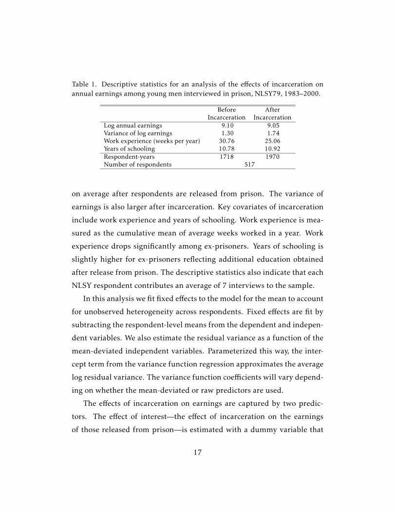
Table 1. Descriptive statistics for an analysis of the effects of incarceration onannual earnings among young men interviewed in prison, NLSY79, 1983–2000.

Before AfterIncarceration Incarceration

Log annual earnings 9.10 9.05Variance of log earnings 1.30 1.74Work experience (weeks per year) 30.76 25.06Years of schooling 10.78 10.92Respondent-years 1718 1970Number of respondents 517

on average after respondents are released from prison. The variance of

earnings is also larger after incarceration. Key covariates of incarceration

include work experience and years of schooling. Work experience is mea-

sured as the cumulative mean of average weeks worked in a year. Work

experience drops significantly among ex-prisoners. Years of schooling is

slightly higher for ex-prisoners reflecting additional education obtained

after release from prison. The descriptive statistics also indicate that each

NLSY respondent contributes an average of 7 interviews to the sample.

In this analysis we fit fixed effects to the model for the mean to account

for unobserved heterogeneity across respondents. Fixed effects are fit by

subtracting the respondent-level means from the dependent and indepen-

dent variables. We also estimate the residual variance as a function of the

mean-deviated independent variables. Parameterized this way, the inter-

cept term from the variance function regression approximates the average

log residual variance. The variance function coefficients will vary depend-

ing on whether the mean-deviated or raw predictors are used.

The effects of incarceration on earnings are captured by two predic-

tors. The effect of interest—the effect of incarceration on the earnings

of those released from prison—is estimated with a dummy variable that

17

Table 2. Variance function regression results for a fixed effects analysis of logearnings among incarcerated men, NLSY79, 1983–2000. (Standard errors inparentheses.)

REML Bayes

β λ β λIntercept .086 -.147 .085 -.149

(.018) (.027) (.018) (.025)

Previously Incarcerated -.326 .464 -.329 .435(.056) (.086) (.056) (.078)

Currently Incarcerated -.460 .196 -.462 .178(.050) (.076) (.051) (.071)

Years of Schooling .041 -.119 .038 -.107(.032) (.050) (.032) (.042)

Work Experience .010 -.017 .010 -.017(.003) (.004) (.003) (.004)

Note: Model for the mean and variance of log annual earnings also included theeffects of age, local area unemployment, enrollment status, region, urban resi-dence, drug use, union membership, public sector employment and 6 industrycategories. N = 3,688, from 517 respondents.

scores zero in all years up to release from prison, and one thereafter. Be-

cause self-reported earnings tend to be very low in the years a respondent

is incarcerated, we also introduce a dummy variable indicating current

incarceration status.

Like the Monte Carlo results, REML and Bayesian estimates of the re-

gression results are very similar in the NLSY (Table 2). Our interest fo-

cuses on the mean and variance of log earnings for men who have been

incarcerated. The REML estimate indicates incarceration reduces average

annual earnings by about 30 percent (1 − e−.326 = .278). The Bayesian es-timate of this effect and its standard error are almost identical. The vari-

ance function coefficients show that the residual variance in log earnings

is higher after incarceration than before. With the REML estimate, the

18

residual variance of earnings rises by about 60 percent (e0.464 = 1.590).

The Bayesian point estimate is somewhat smaller, but tells a similar sub-

stantive story, that men who have been incarcerated experience greater

variability in earnings.

Against the effects of incarceration, schooling and work experience,

which are associated with higher average earnings, are also associated

with less earnings variability for this sample of predominantly low-skill,

crime-involved, men. Point estimates suggest that each year of schooling

is associated with a 10 percent reduction in the residual variance of earn-

ings inequality. Each week of work experience is associated with a 1.7

percent reduction in the variability of earnings.

In sum, in this sample of incarcerated NLSY respondents, more skilled

respondents tend to have higher than average earnings and less earn-

ings variability. The very low-skilled, including the formerly-incarcerated,

have lower than average earnings and greater variability in earnings. These

results indicate greater earnings insecurity among the less-skilled and

less-experienced.

Decomposing Trends in Inequality

While the parameters of the variance function regression may be sub-

stantively interesting, they can also be used to study trends in inequality.

For a positive variable, Y (Y > 0), inequality is defined as the variance of

y = logY . In the log scale, the variance is a scale invariant measure of in-

equality: multiplying the raw variable by a constant, kY , adds a constant

on the log scale, k+ y, leaving the variance of y unchanged. With a regres-

sion on the log scale, on yi , the variance function coefficients are also scale

invariant. Multiplying Y by a constant shifts only the intercept, β0, of the

19

regression for themean in the log scale. The slope coefficients for themean

and the residuals are unchanged, leaving all the variance coefficients un-

changed by a change in scale. The variance of the log, V = V (logY ), is also

functionally related to several common measures of inequality including

the Gini index, G, where

G = 2Φ([V/2]1/2)− 1,

and Φ(·) is the cumulative distribution function of the standard normaldistribution (Allison 1978, 874). We explore the empirical relationship

between the variance of the log and the Gini index in the application be-

low.2

We use variance function regressions to study trends in inequality by

elaborating a standard variance decomposition recently applied by Lemieux

(2006) to men’s hourly wages. For this decomposition the data are orga-

nized in a table and each observation is assigned to a cell in the cross-

classification of all covariates. With k covariates, with levels c1, c2, . . . , ck,

the covariates define a total of C = c1×c2×. . . ck cells. For example, an earn-ings analysis might include covariates for educationmeasured at three lev-

els (say less than high school, high school, and greater than high school)

and work experience (less than 5 years, 5 to 15 years, and greater than

15 years). The population could then be described by an education-by-

experience table, defining 3 × 3 = 9 groups. With data configured in thisway, between-group inequality describes differences across education-experience

cells, andwithin-group inequality refers to heterogeneity within education-

experience cells.

2For log-normal data, Y ,√V is a general inequality parameter of the kind described

by Jasso and Kotz (2008)

20

More formally, for an outcome, yi = logYi , inequality is measured by

the variance, V . The variance can be expressed as a weighted sum of

group means and variances that yield between-group and within-group

components:

V = B+W,

=C∑

c=1

πcr2c +

C∑

c=1

πcσ2c ,

where the πc are cell proportions, rc = yc − y are deviations of the groupmeans from the grand mean, and the σ2c are the variances of yi for each

cell.

With data at two points in time, t = 0,1, we write the cell proportions,

πtc, cell residuals, rtc, and cell variances, σ2tc. The change in the variance of

y from t = 0 to t = 1 can be decomposed into changes in the between-group

and within-group variance. The change in the between-group variance

can be written,

B1 −B0 =C∑

c=1

(π1c −π0c)r21c +C∑

c=1

(r21c − r20c)π0c,

where the first term,∑c(π1c − π0c)r21c, describes a compositional effect—

the change in variance due to shifts in the relative size of population sub-

groups, π1c −π0c. The second term,∑c(r21c − r20c)π0c, is the between-group

effect—the change in the variance due to shifts in group means, r21c − r20c.The change in the within-group variance can similarly be written,

W1 −W0 =C∑

c=1

(π1c −π0c)σ21c +C∑

c=1

(σ21c −σ20c)π0c.

With these expressions, changes in the variance of y can be written as the

21

sum of three components:

V1 −V0 = δC + δB + δW

where the total compositional effect reflecting shifts in the size of popula-

tion subgroups is

δC =C∑

c=1

(π1c −π0c)(r21c +σ21c),

the between-group effect is,

δB =C∑

c=1

π0c(r21c − r20c),

and the within-group effect is,

δW =C∑

c=1

π0c(σ21c −σ20c).

With a time series, t = 0, . . . ,T , it is also useful to plot adjusted variances

that fix at t = 0 either the population proportions,

VCt =C∑

c=1

π0c(r2tc +σ2tc),

the group means,

VBt =C∑

c=1

πtc(r20c +σ2tc),

or the group variances,

VWt =C∑

c=1

πtc(r2tc +σ20c).

These adjusted variances can be interpreted as (1) the variance we would

observe, VCt , if the composition of the population had remained unchanged

22

from t = 0, (2) the variance, VBt , we would observe if group means were

unchanged, and (3) the variance we would observe, VWt , if within-group

variances remained unchanged. In principle, neither the variance decom-

position nor the adjusted variances require a regression model. As in

Lemieux’s (2006) decomposition, the analysis requires only cell propor-

tions, cell means, and cell variances for all years.

Variance function regressions develop the standard decomposition in

three ways. First, we are often interested in studying shifts in inequal-

ity associated with individual covariates. Indeed regression methods have

often been used to decompose the change in variance in this way (e.g.,

Hauser and Xie 2005; Lam and Levison 1992). The extension here in-

volves writing the residual variance as a function of covariates, allowing

the researcher to isolate changes in between-group and within-group in-

equality associated with individual variables. Second, data may be sparse,

so cells observed in some years may be unobserved in others. Regression

estimates can be used to impute means and variances for empty cells, en-

suring that adjusted variances are always defined. More generally, a model

for cells means and variances will smooth the data, reducing the influence

of outlying cells with few observations. Finally, with Bayesian posterior

simulation, bounds can easily be constructed for decomposition quanti-

ties. (Posterior simulation for the usual homoscedastic regression could

also be used to construct inferences for nonstandard decomposition quan-

tities.)

The effect of predictor x on changes in inequality in y can be quantified

with an adjusted variance that fixes a regression coefficient at its value at

the baseline, t = 0. At time t, we have an n × k matrix of covariates, Z t,and a variable of interest given by the n×1 vector, xt. With an n×1 vector

23

of observations on the dependent variable, yt = logYt, write a variance-

function model:

yt = Z tγt + βtxt, and

logσ2t = Z tθt +λtxt.

To assess the effects of x on between-group inequality, construct the ad-

justed variance:

Vβt =

C∑

c=1

πtc(r2tc +σ2tc).

With zc and xc indicating cell c, the adjusted between-group residual, rtc =

ytc − yt, is calculated from

ytc = z′cγt + β0xc.

Here, the adjusted between-group mean at time t is based on all coeffi-

cients at time t, except for the variable of interest, x, where we fix the

coefficient at the baseline, t = 0. The adjusted variance, V βt , can be inter-

preted as the variance we would observe if the between-group coefficient

for x had remained fixed at the baseline time point, t = 0. Similarly, an

adjusted variance that describes the effect of x on within-group inequality

is given by,

V λt =C∑

c=1

πtc(r2tc + σ2tc).

where σ2tc = exp(z′cθt+λ0xc). The adjusted variance, Vλt , can be interpreted

as the variance we would observe if the effects of x on within-group in-

equality had remained fixed at the baseline time point, t = 0. For ex-

ample, a large literature on increasing earnings inequality in the United

States examines the growth in relative earnings of college graduates. Ad-

justed variances, V βt , could show the contribution of the growth in relative

24

earnings of college graduates to the overall rise in inequality. Theories of

labor market deinstitutionalization predict increasing earnings inequal-

ity among poorly-educated workers (e.g., McCall 2000; Sørensen 2000).

Within-group inequality among low-skill workers could be studied with

V λt which fixes educational difference in residual variance at the baseline

time point.

The method can be generalized to study a wide range of effects. For

example, interest may focus on the effects of covariates on only between-

group or within-group inequality. In this case, just the relevant β or λ

coefficients would be fixed at the baseline time point. Adjusted variances

could also be constructed to study the effects of several covariates instead

of just one.

Compositional changes can be studied by fixing the marginal distribu-

tion of individual covariates at the baseline time point. At time t, for each

cell c, the covariate xt has marginal probability p(xtc) = ptc. For example,

let xt be a dummy variable with a mean of .7. Then ptc=.3 for cells in

which xtc = 0, and ptc = .7 for cells in which xtc = 1. The effects of com-

positional shifts in xt on inequality can be estimated by an adjusted set of

cell proportions,

π1c = (p0c/p1c)π1c.

Again, our analysis has parallels in Lemieux’s (2006) analysis of compo-

sitional effects on the residual variance of men’s wages. Lemieux (2006)

proposes a reweighting scheme based on the joint distribution of all co-

variates, not a single covariate of interest. In the current approach, ad-

justed cell proportions preserve the joint distribution of the population

conditional on xt, but inherit the marginal distribution of xt at t = 0. The

25

adjusted cell proportions are then used to form adjusted variances,

Vπt =C∑

c=1

πtc(r2tc +σ2tc).

Similar to the adjusted variances based on fixed regression coefficients, Vπtmight be interpreted as the inequality we would observe if the marginal

distribution of xt were unchanged from t = 0.

Application II: Decomposing Trends in Hourly Wages

A large research literature has examined the growth in inequality in men’s

hourly wages (for reviews and recent contributions see Acemoglu 2002;

Autor, Katz, and Kearney 2005; Lemieux 2006). In this application we

study inequality in the annual wage and salary income for men aged 25 to

55 using data from the March Current Population Survey. We count only

the earnings ofmenworking full-time and year-round, and only those who

report earning at least $100 in a given year. All earnings data have been

adjusted for inflation to 2001 dollars. Inequality in men’s annual earnings

from 1970 to 2005 is shown in Figure 1. In our variance-function analysis,

inequality is measured by the variance in log annual earnings. The vari-

ance of log earnings is compared to the ratio of 90th to the 10th percentile

in raw earnings. The variance and 90/10 ratios have been scaled to equal

1 in 1970. Earnings inequality increases in similar proportion with both

measures. The third series in Figure 1 shows the Gini index for annual

earnings. Because the Gini is a square root function of the variance of the

log, the variance increases more quickly than the Gini when sufficiently

large.3

3Analysis of the derivative, dG/dV shows that the variance increases more quicklythan the Gini (dG/dV < 1) when V > .075 approximately.

26

●

●

●

●

●

●

●●

● ● ●

●

●

●

●

●

●●

●

●

●

●

● ●●

●

●

●

●

●●

●

●

●

●

●

1970 1975 1980 1985 1990 1995 2000 2005

1.0

1.1

1.2

1.3

1.4

1.5

1.6

Earn

ings

Ineq

uality

●

●

●

●

● ●

●

●●

●

●

●●

●

●

●

●

●

●

●

● ● ●●

●

● ● ● ●

●

● ●

●●

● ●

●

●

Variance of Log Earnings90/10 Ratio of EarningsGini Index of Earnings

Figure 1. Trends in earnings inequality, full-time full-year men, aged 25 to 55,1970-2005, March Current Population Survey.

27

Research has focused on earnings inequality by levels of education and

the growth of the residual variance in earnings. Studies of educational

differences in incomes focus on the rising relative pay of college-educated

workers. In 1970, college graduates earned about 35 percent more than

high school graduates. By 2006, the wage advantage of college graduates

had increased to 60 percent. Much of the empirical research analyzed

trends in the education gradient, estimated with a regression of log earn-

ings on years of schooling, typically controlling for experience and other

covariates (Levy and Murnane 1992; Katz and Murphy 1992). The vari-

ance function analysis extends this research by calculating the contribu-

tions to overall earnings inequality of (1) between-group educational in-

equality in earnings, (2) within-group educational inequality in earnings,

(3) the educational composition of the labor force. Groups in this analysis

are defined by race, experience, and education. The analysis synthesizes

the emphasis in economic research on between-group inequality by levels

of education and sociological emphasis on within-group inequality among

low-education workers.

With survey data on year t (t = 1970,1971, . . . ,2005), a variance func-

tion regression on log earnings is written,

yti = x′tiγt + e′tiβt, and

logσ2ti = x′tiθt + e

′tiλt, where

xti is a vector of dummy variables indicating race and ethnicity, and ex-

perience categories, and eti is a 4× 1 vector of dummy variables coded for5 educational categories: (1) less than tenth grade, (2) tenth or eleventh

grade, (3) high school graduate or equivalent, (4) some college, and (5)

four-year degree or more. Four adjusted variances can be constructed with

28

this model to study the effects of education on the trend in earnings in-

equality. The first fixes between-group educational inequality in earnings

at the 1970 level:

Vβt =

C∑

c=1

πtc(r2tc +σ2tc), (1)

where rtc = ytc− yt, yct = x′cγt+e′cβ1970, and xc and ec are design vectors cor-responding to cell c of the race by experience by education table. The sec-

ond adjusted variance fixes within-group educational inequality in earn-

ings:

V λt =C∑

c=1

πtc(r2tc + σ2tc),

where log σ2tc = x′cθt + e′cλ1970. The third adjusted variance combines the

effects of educational inequalities in within-group and between-group in-

equalities:

Vβλt =

C∑

c=1

πtc(r2tc + σ2tc),

The fourth adjusted variance fixes the marginal distribution of education

at the 1970 level:

Vπt =C∑

c=1

πtc(r2tc +σ2tc),

where πtc = (p1970c/ptc)πtc where ptc is the marginal probability of educa-

tion in year t in cell c.

Figure 2 shows the effects of education on the trend in US earnings

inequality. The top panel compares three adjusted variances that fix edu-

cation coefficients at the 1970 level. Observed inequality in earnings in-

creases by 60 percent from 1970 to 2005, but the trend in V βt indicates

that inequality would have increased by only 45 percent if the educational

inequality in mean earnings had remained fixed at the 1970 level. Less

29

research has studied educational differences in within-group inequality

(though see Juhn, Murphy, and Pierce 1993; Lemieux 2006). Trends in

V λt show that differences in the within-group variance across levels of ed-

ucation have affected the rise in US earnings inequality in similar mag-

nitude to the growth in between-group inequality. If the within-group

and between-group effects of education are added together, trends in V βλtshow that they explain about half the growth in US earnings inequality.

Trends in Vπt illustrates the effect of the educational composition of the

workforce (Figure 2b). The adjusted variance tracks the observed vari-

ance, indicating that the great increase in high school graduation rates

and college attendance has had little net distributional effect.

Finally, Figure 3 shows the effects of trends in within-group inequal-

ity. In this case the adjusted variance is obtained by fixing all variance

coefficients, θ and λ, at their 1970 level. With this adjusted variance,

earnings inequality increases by just 25 percent compared to the observed

increase of 60 percent. The adjusted variance indicates that 60 percent,

(60−25)/60 = .58, of the increase in inequality in men’s earnings US is as-sociated with the growth in within-group inequality. In sum, although the

effect of education on between-group inequality has been the main focus

of research, the variance function analysis suggests that educational dif-

ferences in within-group inequality contributes at least as much, and the

overall growth in within-group explains more than half the rise inequality

from 1970 to 2005.

The decomposition analysis can be taken further by reporting infer-

ences about key quantities. Often, inferences are not provided in de-

composition analyses, though sampling error is certainly present. This

seems partly driven by convenience. Inferential statistics for the change

30

1970 1975 1980 1985 1990 1995 2000 2005

0.8

1.0

1.2

1.4

1.6

(a) Observed and Adjusted Variances

Tota

l Var

ianc

e

●

● ●●

●●

●

●

●●

●●

●

●

●●

● ●

●

● ●

●

●● ●

●

●

●

●●

●

●

●

●

●

●

●

●

●

●

● ●

●●

●●

●

●

●

●

●

●

●●

●

● ● ●●

●●

●

● ●

●

● ●

● ●

●

●

●

●

●

Observed varianceββe fixed at 1970λλe fixed at 1970ββe and λλe fixed at 1970

●

● ●

●

●●

●

●

●

●●

●

●

●

●●

● ●

●

●●

●

●●

●

●

●

●

●●

●

●

●

●

●

●

1970 1975 1980 1985 1990 1995 2000 2005

0.8

1.0

1.2

1.4

1.6

(b) Adjusted Variance with Fixed Weights

Tota

l Var

ianc

e

●

● ●

●

●●

●

●●

● ●

●

●

●

●

● ●●

● ●

●●

●

●

●

●

●

●

●

●

●

●

●

●

●

●

●

●

Observed variance1970 education weights

Figure 2. (a) Observed variance of log earnings, and adjusted variances fixingwithin-group and between-group education coefficients at 1970; (b) observedvariance of log earnings and adjusted variance fixing educational attainment atthe 1970, full-time full-year men, aged 25 to 55, 1970–2005.31

●

● ●

●

●●

●

●

●

●●

●

●

●

●●

● ●

●

●●

●

●●

●

●

●

●

●●

●

●

●

●

●

●

1970 1975 1980 1985 1990 1995 2000 2005

0.8

1.0

1.2

1.4

1.6

Tota

l Var

ianc

e

●● ● ●

● ● ● ●

● ●●

●

●●

● ●

●●

●●

● ●●

●

●

●

●

● ●● ●

● ● ●●

●

●

●

Observed variance1970 within−group variance

Figure 3. Observed variance in log earnings, and adjusted variance fixing vari-ance coefficients, λ, at 1970, full-time full-year men, aged 25 to 55, 1970–2005.

32

in adjusted variances are nonstandard calculations, unavailable in stan-

dard statistical packages. Still, the Bayesian analysis provides draws from

the posterior distributions for all the regression coefficients. Output from

posterior simulation can be used to construct standard errors and inter-

vals for the decomposition quantities.

Draws from the posterior distribution of coefficients can be plugged

into the decomposition equation to obtain standard errors and confidence

intervals for the adjusted variance. In equation (1) above, we could write

Vβt (γt,β1970) indicating the dependence of the adjusted variance on 1970

education coefficients and the race and experience coefficients for year t.

With draws from the posterior, written γ∗t and β∗1970, a draw from the

posterior adjusted variance is obtained with the simulated coefficients,

Vβt (γ∗t ,β

∗1970). MCMC output consisting of D draws from the posterior

distributions for the mean and variance regression coefficients yields D

draws from the posterior adjusted variance. The standard error of the

adjusted variance is estimated by the standard deviation of the D draws

from the posterior. Inferences for the adjusted variances, V λt and Vπt , can

be calculated in similar fashion, by plugging in the simulated values of

the regression coefficients, producing posterior draws from the adjusted

variance.

Table 3 reports the effects of the change in the education coefficients, β

and λ, the compositional effects of changes in educational attainment, and

the effects of changes in within-group inequality on the growth in earnings

inequality from 1970 to 20005. Standard errors calculated from posterior

simulation are reported in parentheses. The change in variance is obtained

by subtracting the observed 1970 variance from the 2005 observed and ad-

justed variance. To calculate inference for the change in variance, subtract

33

Table 3. Observed and adjusted variances, full-time, full-year men’s log annualearnings, CPS 1970-2005. Standard errors in parentheses are calculated withMCMC posterior simulation.

Change from Percent of2005 1970 to 2005 Change Explained

Observed Variance .481 .179 -(.004) (.004)

Adjusted variance, fixing at 1970:Education effects, β .432 .131 27.2

(.004) (.004)Education effects, β and λ .387 .085 52.5

(.006) (.006)Educational attainment .500 .199 -10.8

(.006) (.004)All within-group effects, θ and λ .371 .069 61.4

(.005) (.003)

the posterior draws from 1970 variance from the posterior draws from the

2005 variance. Results show that the standard errors are extremely small

compared to the change in variance indicating that the overall growth in

inequality and the growth attributable education effects and within group

inequality is unlikely to be due to sampling error.

Though our analysis is based on annual earnings for full-time full-

year male workers, different data and samples may yield different results.

For example, Lemieux (2006) reports large composition effects related to

workforce aging in his decomposition analysis of within-group inequality

in hourly wages in the Outgoing Rotation Group files of the CPS. We find

little evidence of the composition effects of schooling and larger effects of

schooling coefficients on between-group and within-group inequality in

the March CPS annual earnings data. This divergence suggests the sensi-

tivity of results to the range of plausible design choices.

34

Discussion

In this paper we proposed a variance function regression for studying

the level and trend in inequality. By writing a regression model for both

the mean and variance of a dependent variable, the variance function re-

gression treats within-group, or residual, inequality as a something to be

explained. In previous research on earnings, the within-group variance

was interpreted to reflect the influence of returns to unobserved charac-

teristics. Theories of inequality have also treated with-group inequality

as measuring risk or insecurity. Our analysis provides a way of explain-

ing variability in risk or insecurity in addition to the usual account of

between-group inequality. We also extended the model to a variance de-

composition of the change in inequality, where the variance function al-

lows us to study the effects of covariates on bothwithin-group and between-

group inequality.

The model can be estimated using standard software. A two-stage

estimator—consisting of a least squares fit for the mean and a gamma re-

gression on the log squared residuals—provides accurate point estimates.

Maximum likelihood estimates can be obtained by iterating between the

linear regression and the gamma regression. Bayesian MCMC estimation

yields draws from the full posterior distribution, producing inferences

about variance decomposition.

The model was illustrated in two applications: an analysis of earnings

among incarcerated respondents in the NLSY79, and an analysis of earn-

ings inequality among US male workers from 1970 to 2005. The analysis

of NLSY prisoners showed that incarceration was associated with not just

reduced earnings, but also an increase in the variability of earnings. Anal-

ysis of the 35-year trend in men’s earnings inequality showed that half

35

of the growth in inequality is due to rising between-group and within-

group inequality by levels of education. Half of the growth in inequality

is associated with the growth in within-group inequality. Changes in the

educational composition of the male workforce was found to contribute

very little to the growth in earnings inequality.

Variance function regressions offer a more complete model of inequal-

ity but researchers should carefully consider the model specification and

measurement for this two-equation analysis. Parameterizing the mean

and the variance multiplies misspecification errors. Specification errors in

themodel for themean—perhaps due to omitted variables or nonlinearities—

obviously results in biased estimates of the mean coefficients. In addition,

however, because the residuals are biased estimates of the true errors, co-

efficients for the variance will generally be biased as well, even if the vari-

ance equation is correctly specified. If the variance equation is misspec-

ified, but the mean equation is correctly specified, the standard errors of

mean regression coefficients will also be biased. However, point estimates

of the mean regression coefficients will be unbiased, despite misspecifi-

cation of the variance regression.4 Measurement error in the dependent

variable will also affect the interpretation of the results. In particular clas-

sical measurement error will bias the intercept of the variance equation,

though other coefficients will be unaffected. The variance coefficients will

be biased, of course, if measurement error in the dependent variable is

correlated with the independent variables. Indeed, the mean coefficients

would be biased too in this situation, just as in the usual linear regression.

The current model could be extended in several ways. In the analysis

4In a correctly specified model for the mean, the errors will have zero expectationensuring the unbiasedness of the ML estimates of β.

36

of discrete outcomes like counts or binary variables, the mean and vari-

ance are often assumed to be functionally related. For example, a binary

dependent variable, y, is often assumed to be Bernoulli where E(y) = p

and V (y) = p(1 − p). An overdispersion parameter is sometimes added tocapture extra-Bernoulli variation, V (y) = φp(1 − p). A variance-functionmodel with a discrete outcome might then write the overdispersion pa-

rameter, φ, as a function of covariates. The model could also be extended

in a Bayesian framework. The Bayesian model could be elaborated to add

random components for both the mean and the variance. Where data are

clustered in small areas like counties or census tracts for example, random

components in the variance function would allow variability in within-

group inequality beyond that explained by the covariates. Such models

could be estimated with MCMC methods for posterior simulation.

Regression analyses of inequality typically capture only differences be-

tween groups. In sociological applications, residual inequality tends to be

very large in comparison to between-group inequality. The substantive

significance of this large residual variance tends to be glossed either by

appealing to the importance of regression coefficients or dismissing resid-

ual variance as the combined effects of measurement error and uncorre-

lated omitted variables. If overall inequality—the overall spread of the

dependent variable—is really the main substantive interest, the variance

function regression provides a useful tool, making the residual variance

itself a target for analysis.

37

Appendix 1: Variance Function MLE’s in Stata

The following Stata code takes a dependent variable, Y, a local macro vari-able listing predictors for the mean, X, and another listing predictors forthe variance, Z. The code monitors the log likelihood and outputs the pa-rameter estimates.

reg Y ‘X’;predict R, r; * OLS resids;gen R2=Rˆ2; * squared resids for glm fit;glm R2 ‘Z’, family(gamma) link(log); * gamma reg on log(r2);predict S2, mu; * fitted variances, exp(Xb);gen LOGLIK=-.5*(ln(S2)+(R2/S2)); * evaluating log likelihood;egen LL0 = sum(LOGLIK); * summing log likelihood;di LL0;

* Updating beta and lambda coefficients;gen DLL=1; * initialize change in loglik;while DLL > .00001 {;drop R;quietly: reg Y ‘X’ [aw=1/S2]; * WLS with variances as weights;drop S2;predict R, r; * WLS resids;replace R2=Rˆ2; * squared resids for glm fit;est store BETA; * saving beta coefs;quietly:glm R2 ‘Z’, family(gamma) link(log); * gamma reg on log(r2);

predict S2, mu; * fitted variances, exp(Xb);est store LAMBDA; * saving lambda coefs;replace LOGLIK=-.5*(ln(S2)+(R2/S2)); * evaluating log likelihood;egen LLN = sum(LOGLIK); * summing log likelihood;di LLN;replace DLL=LLN-LL0; * assess convergence;replace LL0=LLN;drop LLN;

};est table BETA LAMBDA, b se; * table with coefs and se’s

38

Appendix 2: BUGS Code for Variance Function Regression

The following BUGS code was used in the Monte Carlo experiment re-ported in Table 2. The code fits a bivariate regression with dependentvariable, y, and a single predictor x, to simulate from the posterior distri-bution of the mean coefficients, b0 and b1 and the variance coefficients,lambda0 and lambda1.

model {for(i in 1:n) {y[i] ˜ dnorm(mu[i], tau.y[i])mu[i] <- b0 + b1*x[i]tau.y[i] <- 1/sigma2[i]log(sigma2[i]) <- lambda0 + lambda1*x[i]}

lambda0 ˜ dnorm(0, tau.lambda0)lambda1 ˜ dnorm(0, tau.lambda1)tau.lambda0 ˜ dgamma(0.001, 0.001)tau.lambda1 ˜ dgamma(0.001, 0.001)b0 ˜ dnorm(0, 1.0E-6)b1 ˜ dnorm(0, 1.0E-6)

}

39

References

Acemoglu, Daron. 2002. “Technical Change, Inequality, and the LaborMarket.” Journal of Economic Literature 40:70–72.

Aitkin, Murray. 1987. “Modelling Variance Heterogeneity in NormalRegression Using GLIM.” Applied Statistics 36:332–339.

Allison, Paul D. 1978. “Measures of Inequality.” American SociologicalReview 43:865–880.

Anscombe, F.J. 1961. “Examination of Residuals.” In Proceedings of theFourth Berkeley Symposium on Mathematical Statistics and Probability,volume 1, pp. 1–36, Berkeley, CA. University of California Press.

Arden, Rosalind and Robert Plomin. 2006. “Sex Differences in Varianceof Intelligence Across Childhood.” Personality and Individual Differ-ences 41:39–48.

Autor, David H., Lawrence F. Katz, and Melissa S. Kearney. 2005.“Trends in U.S. Wage Inequality: Re-Assessing the Revisionists.” Na-tional Bureau of Economic ResearchWorking Paper 11627, NationalBureau of Economic Research, Cambridge, MA.

Blau, Peter M. and Otis Dudley Duncan. 1967. The American Occupa-tional Structure. New York: Free Press.

Budig, Michelle J and Paula England. 2001. “The Wage Penalty forMotherhood.” American Sociological Review 66:204– 225.

Cancio, A. Silvia, T. David Evans, and David J. Maume. 1996. “Recon-sidering the Declining Significance of Race: Racial Differences inEarly Career Wages.” American Sociological Review 61:541–556.

Cook, R.D. and S. Weisberg. 1983. “Diagnostics for Heteroscedasticityin Regression.” Biometrika 76:1–10.

DiNardo, James, Nicole M. Fortin, and Thomas Lemieux. 1996. “La-bor Market Institutions and the Distribution of Wages, 1973-1992.”Econometrica 64:1001–44.

40

Edwards, Jode W. and Jean-Luc Jannink. 2006. “Bayesian Modellingof Heterogeneous Error and Genotypic × Environment InteractionVariables.” Crop Breeding Genetics and Cytology 46:820–833.

Harvey, Andrew C. 1976. “Estimating Regression Models with Multi-plicative Heteroscedasticity.” Econometrica 44:461–465.

Hauser, Seth M. and Yu Xie. 2005. “Temporal and regional variation inearnings inequality: urban China in transition between 1988 and1995.” Social Science Research 34:44–79.

Jasso, Guillermina and Samuel Kotz. 2008. “Two Types of Inequality:Inequality between Persons and Inequality Between Subgroups.” So-ciological Methods and Research 37:31–74.

Jencks, Christopher, Marshall Smith, Henry Acland, Mary Jo Bane, Bar-bara Heyns, and Stephan Michelson. 1972. Inequality: A Reassess-ment of the Effect of Family and Schooling in America. New York:Harper.

Juhn, Chinhui, Kevin M. Murphy, and Brooks Pierce. 1993. “Wage In-equality and the Rise in Returns to Skill.” Journal of Political Economy101:410–442.

Katz, Lawrence F. and Kevin M. Murphy. 1992. “Changes in RelativeWages, 1963–1987: Supply and Demand Factors.” Quarterly Journalof Economics 107:35–78.

Kim, Chang Hwan and Arthur Sakamoto. 2008. “The Rise of Intra-Occupational Wage Inequality in the United States, 1983 to 2002.”American Sociological Review 73:129–157.

Kling, Jeffrey R. 2006. “Incarceration Length, Employment, and Earn-ings.” American Economic Review 96:863–876.

Lam, David and Deborah Levison. 1992. “Age, Experience, and School-ing: Decomposing Earnings Inequality in the United States andBrazil.” Sociological Inquiry 62:220–245.

Lemieux, Thomas. 2006. “Increasing Residual Wage Inequality: Com-position Effects, Noisy Data, or Rising Demand for Skill?” AmericanEconomic Review 96:461–498.

Levy, Frank and Richard J. Murnane. 1992. “U.S. Earnings Levels and

41

Earnings Inequality: A Review of Recent Trends and Proposed Ex-planations.” Journal of Economic Literature 30:1333–1381.

Lewis, Matthew. 2008. “Price Dispersion and Competition with Differ-entialed Sellers.” Journal of Industrial Economics 56:654–678.

Massey, Douglas S. 2007. Categorically Unequal: the American Stratifica-tion System. New York, NY: Russell Sage Foundation.

McCall, Leslie. 2000. “Explaining Levels of Within-Group Wage In-equality in U.S. Labor Markets.” Demography 37:415–430.

Minto, Colin, Ransom A. Myers, and Wade Blanchard. 2008. “SurvivalVariability and Population Density.” Nature 452:344–348.

Nelder, John A. and Y. Lee. 1991. “Generalized Linear Models for theAnalysis of Taguchi-Type Experiments.” Applied Stochastic Modelsand Data Analysis 7:107–120.

Pager, Devah. 2003. “The Mark of a Criminal Record.” American Journalof Sociology 108:937–975.

Park, R.E. 1966. “Estimation with Heteroscedastic Error Terms.” Econo-metrica 34:888.

Selb, Peter. 2008. “Supersized Votes: Ballot Length, Uncertainty, andChoice in Direct Legislation Elections.” Public Choice 135:319–336.

Smyth, Gordon K. 2002. “An Efficient Algorithm for REML in Het-eroscedastic Regression.” Journal of Graphical and CompuationalStatistics 11:836–847.

Smyth, Gordon K., A. Frederik Huele, and Arunas P. Verbyla. 2001. “Ex-act and Approximate REML for Heteroscedastic Regression.” Statis-tical Modelling 1:161–175.

Sørensen, Aage B. 2000. “A Sounder Basis for Class Analysis.” AmericanJournal of Sociology 105:1523–1558.

Sørensen, Jesper B. and Olav Sorenson. 2007. “Corporate Demographyand Income Inequality.” American Sociological Review 72:766–783.

Tilly, Charles. 1998. Durable Inequality. Berkeley, CA: University of Cal-ifornia Press.

Verbyla, A.P. 1993. “Modelling Variance Heterogeneity: Residual Max-imum Likelihood and Diagnostics.” Journal of the Royal StatisticalSociety Series B 55:493–508.

42

Western, Bruce. 2002. “The Impact of Incarceration on Wage Mobilityand Inequality.” American Sociological Review 67:526–546.

Western, Bruce. 2006. Punishment and Inequality in America. New York:Russell Sage Foundation.

43