Variance estimation of modal parameters from …Variance estimation of modal parameters from...

HAL Id: hal-01328435https://hal.inria.fr/hal-01328435

Submitted on 8 Jun 2016

HAL is a multi-disciplinary open accessarchive for the deposit and dissemination of sci-entific research documents, whether they are pub-lished or not. The documents may come fromteaching and research institutions in France orabroad, or from public or private research centers.

L’archive ouverte pluridisciplinaire HAL, estdestinée au dépôt et à la diffusion de documentsscientifiques de niveau recherche, publiés ou non,émanant des établissements d’enseignement et derecherche français ou étrangers, des laboratoirespublics ou privés.

Variance estimation of modal parameters fromoutput-only and input/output subspace-based system

identificationPhilippe Mellinger, Michael Döhler, Laurent Mevel

To cite this version:Philippe Mellinger, Michael Döhler, Laurent Mevel. Variance estimation of modal parameters fromoutput-only and input/output subspace-based system identification. Journal of Sound and Vibration,Elsevier, 2016, 379, pp.1-27. 10.1016/j.jsv.2016.05.037. hal-01328435

https://hal.inria.fr/hal-01328435

https://hal.archives-ouvertes.fr

Variance estimation of modal parameters from output-only and input/outputsubspace-based system identification

Philippe Mellinger, Michael Dohler∗, Laurent Mevel

Inria / IFSTTAR, I4S, Campus de Beaulieu, 35042 Rennes, France

Abstract

An important step in the operational modal analysis of a structure is to infer on its dynamic behavior through its modal

parameters. They can be estimated by various modal identification algorithms that fit a theoretical model to measured

data. When output-only data is available, i.e. measured responses of the structure, frequencies, damping ratios and

mode shapes can be identified assuming that ambient sources like wind or traffic excite the system sufficiently. When

also input data is available, i.e. signals used to excite the structure, input/output identification algorithms are used. The

use of input information usually provides better modal estimates in a desired frequency range. While the identification

of the modal mass is not considered in this paper, we focus on the estimation of the frequencies, damping ratios and

mode shapes, relevant for example for modal analysis during in-flight monitoring of aircrafts. When identifying

the modal parameters from noisy measurement data, the information on their uncertainty is most relevant. In this

paper, new variance computation schemes for modal parameters are developed for four subspace algorithms, including

output-only and input/output methods, as well as data-driven and covariance-driven methods. For the input/output

methods, the known inputs are considered as realizations of a stochastic process. Based on Monte Carlo validations,

the quality of identification, accuracy of variance estimations and sensor noise robustness are discussed. Finally these

algorithms are applied on real measured data obtained during vibrations tests of an aircraft.

Keywords: (Operational) modal analysis, Subspace algorithms, Variance estimation, Aircraft application

1. Introduction

The design and maintenance of mechanical, aeronautical or civil structures subject to noise and vibrations are

an important topic in structural engineering. Laboratory and in-operation vibration tests are performed on structures

for a modal analysis [1]. The desired modal parameters (frequencies, damping ratios, mode shapes) are related to

the poles and observed eigenvectors of a linear time-invariant system. Subspace-based linear system identification

algorithms have been proven efficient for the identification of such systems, fitting a linear model to either output-

only measurements or input and output measurements taken from a system [2]. Usually, ambient excitation sources

∗Corresponding author. Tel: +33 2 99 84 22 25.Email addresses: [email protected] (Philippe Mellinger), [email protected] (Michael Dohler),

[email protected] (Laurent Mevel)

Preprint submitted to Journal of Sound and Vibration April 20, 2016

(e.g. wind, traffic) act on a structure during real tests. Besides these non-measurable excitation sources, in addition

some measurable excitation sources (e.g. artificial excitation from hammer impact or shaker, ground motion) may be

available. Thus, inputs to the considered system are in general unknown, but in some cases, some known inputs may

be available in addition to the unknown inputs.

Operational Modal Analysis (OMA) refers to the identification of modal parameters from output-only measure-

ments under unknown ambient excitation. In Operational Modal Analysis with eXogenous inputs (OMAX), some

known or measured excitation is applied to the structure besides the ambient noise. Throughout this paper, the known

input sequence is assumed to be a realization of a stochastic process. For example, control surface excitations can

be used during either flight or ground vibration tests in the particular case of an aircraft. A stochastic framework

can model the excitation of flaps actioned by a pilot during in-flight vibration tests, which are the known inputs in

this case. Other unknown ambient excitation has to be considered, which is commonly assumed to be white noise.

The measured outputs are due to both known and unknown inputs, and may be corrupted by noise (i.e. sensor noise

uncorrelated with known inputs).

Many methods for OMA and OMAX are available in the literature [3]. In this work, we focus on subspace

methods. By appropriate projections of the measurement data [2], the state space representation of the corresponding

linear system is properly estimated. Then, the modal parameters are retrieved from the estimated state space model.

There are a variety of subspace algorithms, which are defined by the way the measurements are projected. Data-driven

subspace algorithms are characterized by large Hankel matrices filled with raw data. Orthogonal or oblique projections

are carried out on their row space [2, 4], for which numerical schemes with the QR decomposition [2] and iterative

and fast approaches [5–7] have been studied. In the stochastic framework, those projectors are essentially conditional

expectations of the future output data with respect to some instrument depending on the algorithm [8]. Connections

with Prediction Error Methods [9] and closed loop identification have been investigated [10–12]. It is well understood

that the projections in the data-driven methods can be partly expressed in terms of auto- and cross-covariances of

the respective time series [2, 13]. The class of covariance-driven subspace algorithms is purely based on auto- and

cross-covariance matrices of the measurements and has been used for modal identification [14] or damage detection

[15, 16] using vibration data for more than a decade. Like with data-driven methods, covariance-driven methods can

be based on output-only data or input/output data [13, 17–20].

The purpose of this paper is the variance analysis of modal parameters obtained from subspace methods. Using

noisy measurement data, subspace algorithms provide parameter estimates that are afflicted with statistical uncertainty

due to finite data, unknown inputs and sensor noise properties. In-depth asymptotic variance analyses for subspace

algorithms have been carried out in the automatic control literature [21–24], which are of important theoretical value.

In these works, analytical expressions for the asymptotic covariance of the system matrices are derived for several

output-only and input/output subspace algorithms. However, explicit expressions for the actual covariance estimation

from measurements are not available therein.

In the field of vibration analysis, such explicit expressions have been proposed for some subspace methods. For

2

example, an application of the variance analysis in [21] for input/output subspace identification was tempted in [25]

in the context of modal analysis, however without entirely satisfying results according to the authors of the study.

A different and successful approach was developed in [26], where an estimated covariance on the measurements is

propagated to the desired parameters based on a sensitivity analysis. The required sensitivities are derived analytically

through the propagation of a first-order perturbation from the data to the identified parameters. This approach has the

advantage of computational convenience: the sample covariance as the starting point is directly linked to the measure-

ments and therefore easy to compute, and the sensitivities are computed using the system identification estimates. In

[27], details of this scheme are developed for the covariance computation for output-only covariance-driven subspace

identification. This approach offers advantages beyond technical correctness. The exploitation of the stabilization

diagram, which is a basic tool for OMA(X), is a crucial step in modal analysis, but computationally costly for the

covariance computation. A well-adapted fast and memory efficient implementation in an operational modal analysis

context has been proposed in the covariance-driven output-only case [28]. As a result, the computational cost for

the variance computation of an entire stabilization diagram analysis is reduced significantly. This was mandatory

for realistic applications on large structures like in [29, 30] and a prerequisite for implementation in modal analysis

software.

While this approach has shown to be working both in theory and practice for the variance computation of modal

parameters, it is only available for output-only covariance-driven subspace identification [27, 28]. In the present

paper, this covariance computation approach is generalized to a wider class of subspace algorithms in both output-

only and input/output frameworks, and for covariance-driven and data-driven methods, while keeping the advantages

of the previously published method in [28] in terms of efficiency and precision. Notice that, while the computation

of the modal mass is possible with the input/output algorithms [31], we focus on the covariance computation for

frequencies, damping ratios and mode shapes. In this paper, new covariance computation schemes are developed for

four well-known subspace algorithms. One of them is an output-only algorithm:

• Output-only orthogonal projection data-driven, which is the UPC algorithm (Unweighted Principal Component)

[2, Sec. 3.3.2], [14].

Furthermore, we consider three input/output algorithms:

• Input/output covariance-driven [32],

• Input/output orthogonal projection data-driven, related to the projection algorithm [2, Sec. 2.3.2] and MOESP

(Multivariable Output Error State Space) [33], and

• Input/output oblique projection data-driven, which is the N4SID algorithm (Numerical algorithms for Subspace

State Space System IDentification) [2, 34].

The extension from the output-only covariance-driven algorithm to these four subspace algorithms is performed by a

thorough sensitivity analysis of the underlying auto- and cross-covariance matrices in the formulation of the subspace

3

algorithms. In particular, the extension to the data-driven algorithms is carried out by developing an equivalent

formulation in a covariance-driven form, regarding the estimation of frequencies, damping ratios and mode shapes.

The new algorithms are validated in extensive Monte-Carlo simulations and in an application on an aircraft.

This paper is organized as follows. In Section 2, the underlying vibration modeling is recalled. In Section 3, the

general properties of subspace identification algorithms are described and the five considered subspace algorithms are

detailed. An equivalent covariance-driven formulation of the data-driven algorithms is discussed in Section 4, which

is the basis for the subsequent derivation of the covariance computation for the data-driven algorithms. Then variances

for the considered algorithms are derived in Section 5. The validation of the methods in Monte-Carlo simulations is

presented in Section 6 in an academic example. The application on an aircraft structure is presented in Sections 7 and

8 using simulations and real data, respectively, before discussing and concluding the paper in Sections 9 and 10.

Nomenclature

⊗ Kronecker product n system order

vec column stacking vectorization operator N data length

† Moore-Penrose pseudoinverse Ni,No number of inputs, outputs

Y/X orthogonal projection nb number of data blocks

Y/Z X oblique projection H∗ subspace matrix for the methods:

πX orthogonal projector on X OOcov output-only covariance-driven

X⊥ orthogonal complement of X OOort output-only orthogonal projection data-driven

E expectation IOcov input/output covariance-driven

R set of real numbers IOort input/output orthogonal projection data-driven

∆X first order perturbation on X IOobl input/output oblique projection data-driven

ΣX covariance of vec(X) Γp observability matrix

JY,X sensitivity of vec(Y) wrt. vec(X) (·)−, (·)+ past and future time horizon

Ia identity matrix of size a × a q, p length of past and future time horizon

0a,b zero matrix of size a × b U−,U+ data Hankel matrices of inputs

Pa,b permutation, vec(XT ) = Pa,bvec(X) Y−,Y+ data Hankel matrices of outputs

A,C state transition, output matrices W− stacked matrix ofU− and Y−

B,D output, feedthrough matrices U−, U+ data Hankel matrices of unknown inputs

uk, yk known inputs, outputs V−,V+ data Hankel matrices of sensor noise

uk, vk unknown inputs, sensor noise Ri auto- or cross-covariance matrix

fi, ξi frequency, damping ratio

4

2. Vibration modeling

2.1. Mechanical and state space models

The vibration behavior of a linear time-invariant mechanical structure, which is observed at some sensor positions,

can be described by the equations [1] Mq(t) + Cq(t) +Kq(t) = F u(t) + u(t)

y(t) = Laq(t) + Lvq(t) + Ldq(t) + v(t)(1)

whereM, C andK ∈ Rm×m are mass, stiffness and damping matrices, and m is the number of degrees of freedom. The

vector q(t) ∈ Rm×1 contains the displacements at the degrees of freedom generated by the known inputs u(t) ∈ RNi ×1

and unknown inputs u(t) ∈ Rm×1, where Ni is the number of known inputs, and F ∈ Rm×Ni represents how the known

inputs are applied to the system. The vector y(t) ∈ RNo×1 contains the observed outputs, with No being the number of

sensors. The matrices La, Lv and Ld ∈ RNo×m represent how accelerations, velocities and displacements are obtained

from the model degrees of freedom. The vector v(t) ∈ RNo×1 is the sensor noise. Both u(t) and v(t) are assumed to be

white noise with finite fourth moments and uncorrelated with the known inputs [2, 35].

From Eq. (1), the following continuous-time state space model can be obtained: x(t) = Acx(t) + Bcu(t) + Bcu(t)

y(t) = Ccx(t) + Dcu(t) + Dcu(t) + v(t),(2)

where x(t) = [q(t)T q(t)T ]T ∈ Rn×1 is the state vector, n = 2m is the model order and

Ac =

−M−1C −M−1K

Im 0m,m

∈ Rn×n, Bc =

M−1F

0m,Ni

∈ Rn×Ni , Cc =

[Lv − LaM

−1C Ld − LaM−1K

]∈ RNo×n

and Dc = LaM−1F ∈ RNo×Ni are the state transition, input, output and feedthrough matrices, respectively. The

matrices Bc and Dc are defined similarly with respect to the unknown inputs. The matrices Ia ∈ Ra×a and 0a,b ∈ Ra×b

are the identity and the zero matrix, respectively.

Sampling Eq. (2) at rate τ and assuming zero-order hold for inputs u(t) and u(t) yield the discrete-time state space

representation [9] xk+1 = Axk + Buk + Buk

yk = Cxk + Duk + Duk + vk,(3)

where A = eAcτ, B = (A − I)A−1c Bc, B = (A − I)A−1

c Bc, C = Cc, D = Dc, and D = Dc.

The modal parameters of system (1) are equivalently found in system (3) as follows. Let λi and φi be eigenvalues

and eigenvectors of A, for i = 1, . . . , n. Then the poles µi of systems (1) and (2), modal frequencies fi, damping ratios

ξi and mode shapes ϕi are obtained by

µi =log(λi)τ

, fi =|µi|

2π, ξi =

−Re(µi)|µi|

, ϕi = Cφi.

5

2.2. Stochastic nature of known inputs

Until now, no assumption has been stated on the known input ukk=1,...,N for the case of input/output algorithms.

Known inputs are used in what is called deterministic [2] or combined deterministic/stochastic [2, 31] system identi-

fication in the literature. In the designation of these methods, there is equivalence between “deterministic” and “the

input sequence is known”, and between “stochastic” and “there are unknown inputs and/or noise”.

However, these designations should not be mistaken with the nature of the known inputs. The known input

sequence itself may be a deterministic signal, or it may be a realization of a stochastic process. For the considered

input/output methods in this paper, we assume that known inputs are realizations of a stochastic process satisfying

mild ergodicity and mixing properties. This assumption is in particular coherent with the ergodic-algebraic framework

of [35] and cross-covariance estimates in [13] for covariance-driven input/output algorithms. In combination with

standard white noise assumptions for unknown inputs and measurement noise, this assumption allows the consistent

computation of auto-covariances of the inputs, the outputs and of cross-covariances between inputs and outputs, which

is a basic step in subspace identification.

These auto- and cross-covariances contribute to the modal parameter estimates. Then, the corresponding un-

certainties for these auto- and cross-covariances play together in a non-trivial way to obtain the modal parameter

uncertainties, for which the expressions are derived in this paper. Note that assuming known inputs as stochastic is no

contradiction for the particular case of a system with no unknown inputs and no sensor noise. In this case, the modal

parameters can be identified exactly from the known inputs and outputs, and their variance assuming stochastic inputs

is indeed zero, as will be shown in Section 6.

3. Subspace identification

Subspace algorithms are based on projections of output or input/output data Hankel matrices with a “past” and

“future” time horizon. These projections are designed in a way that the column space of the resulting matrix – we

call it subspace matrix H – is defined by the observability matrix Γp = [CT . . . (CAp−1)T ]T of system (3). All five

subspace algorithms considered in this paper have the respective factorization property H = ΓpZ, where Z depends

on the chosen algorithm [2]. This property leads to the estimation of Γp from measurement data and subsequently to

the system matrices A and C, from where the desired modal parameters are identified.

After defining the underlying data Hankel matrices and the respective auto- and cross-covariances, the three

steps of modal identification with subspace algorithms are detailed in this section: 1/ Estimation of auto- and cross-

covariance matrices related to “past” and “future” data matrix products for the chosen subspace algorithm, 2/ Compu-

tation of the subspace matrixH for the five subspace algorithms considered in this paper, and finally 3/ Estimation of

the modal parameters fromH .

6

Definition 1 (Data Hankel matrix [2]). Let Nt samples al ∈ Rr×1 of a discrete signal a be given, and integers i and j

with i ≤ j ≤ Nt − N + 1. Then the data Hankel matrixAi| j is defined as

Ai| jdef=

ai ai+1 . . . ai+N−1

......

. . ....

a j a j+1 . . . a j+N−1

∈ R( j−i+1)r×N .

Let N + p + q be the number of available samples for the known inputs uk and the outputs yk, where q and p are

parameters that define a “past” and “future” time horizon. They are most often equal, and assumed to be large enough

to satisfy the condition min(p − 1)No, qNo ≥ n. Under the above Definition 1, the “past” (−) and “future” (+) data

Hankel matrices containing the known data are defined as in [2],

U−def=

1√

NU0|q−1, U

+ def=

1√

NUq|q+p−1, Y

− def=

1√

NY0|q−1, Y

+ def=

1√

NYq|q+p−1. (4)

Consider similarly the unknown signals, i.e. the unknown input u, the sensor noise v and the state x, defining the

corresponding matrices U− def= 1

√NU0|q−1, U+ def

= 1√

NUq|q+p−1, V− def

= 1√

NV0|q−1, V+ def

= 1√

NVq|q+p−1 and finally

X−def= 1

√NX0|0, X+ def

= 1√

NXq|q, which are needed for deriving the equations of the model. Then Eq. (3) can be

extended to [2] Y− = ΓqX

− + HqU− + HqU

− +V−

Y+ = ΓpX+ + HpU

+ + HpU+ +V+

X+ = AqX− + ∆qU− + ∆qU

−.

(5)

The matrices ∆q, ∆q, Hp and Hp are defined in [2].

3.1. First step: estimation of auto- and cross-covariances

Known data (outputs and, if available, inputs) are used to estimate auto- and cross-covariances in order to compute

the subspace matrix H . Let a and b be placeholders for two of these signals (e.g. u and y, y and y or u and u). Then,

their cross-covariance estimate at lag i is defined as

R[a,b]i =1N

N∑k=1

ak+ibTk , (6)

considering that a and b are ergodic and zero mean random processes. The term auto-covariance is used for the cross-

covariance of the same signal, i.e. a = b in (6). Note that due to the finite data length, these auto- and cross-covariance

estimates are random variables with a covariance [36], which will be the starting point of the variance propagation to

the modal parameter estimates in Section 5.

Besides the direct computation as in Eq. (6), an efficient way to compute auto- and cross-covariance functions

at all lags i is to first estimate the PSD (Power Spectral Density) functions of signals by Welch’s method [9] and to

compute the inverse discrete Fourier transform of the result, using the Fast Fourier Transform (FFT), as detailed in

Appendix A.

7

Using “past” and “future” data Hankel matrices as defined in Eq. (4) brings some useful properties, since their

products are related to the auto- and cross-covariance estimates. For example, it holds

U+Y−T

=

R[u,y]q R[u,y]q−1 . . . R[u,y]1

R[u,y]q+1 R[u,y]q . . . R[u,y]2

......

......

R[u,y]q+p−1 R[u,y]q+p−2 . . . R[u,y]p

, (7)

and similarly

U−Y−T

=

R[u,y]0 R[u,y]−1 . . . R[u,y]1−q

R[u,y]1 R[u,y]0 . . . R[u,y]2−q

......

. . ....

R[u,y]q−1 R[u,y]q−2 . . . R[u,y]0

, U+Y+T

=

R[u,y]0 R[u,y]−1 . . . R[u,y]1−p

R[u,y]1 R[u,y]0 . . . R[u,y]2−p

......

. . ....

R[u,y]p−1 R[u,y]p−2 . . . R[u,y]0

(8)

The products Y−Y−T, Y+Y+T

, Y+Y−T, U−U−

T, U+U+T

and U+U−T

are computed analogously. These products

based on auto- and cross-covariances are elementary blocks for the computation of the subspace matrices needed by

the subspace algorithms of Section 3.2.

Remark 2 (Cross-covariance with unknown inputs and sensor noise). Products between data Hankel matrices con-

taining outputs or known inputs and noise Hankel matrices are established analogously as above. These cross-

covariance based products will appear in the derivation of subspace algorithms in the following section. Some of

these cross-covariances tend to zero due to the assumption that unknown inputs and sensor noise are white and un-

correlated with the known inputs. In particular it holds U+U+T = 0 andV+U+T = 0 for an infinite amount of data.

Under these assumptions, past outputs are uncorrelated with future unknown inputs and with future sensor noise, and

it holds similarly U+Y−T

= 0 and V+Y−T

= 0. These properties are required for the development of the subspace

methods in the next section.

3.2. Second step: computation of subspace matrixH

Each subspace algorithm is related to a subspace matrix H with factorization property H = ΓpZ, where Z

depends on the algorithm. Subspace algorithms may be divided into two families: covariance-driven and data-driven.

Covariance-driven subspace matrices are products of auto- or cross-covariance matrices. Data-driven matrices can be

described as a product of covariance-driven matrices with a data Hankel matrix [8]. The main difference between both

kinds of algorithms is the size of the associated subspace matrix. When the number of samples increases, covariance-

driven matrices converge to their expected value, while their column dimension does not increase. Concerning data-

driven matrices, their covariance components converge as the number of samples increases, but also their column

dimension increases due to the increasing dimension of the data-matrix part. In both cases, the column space of the

respective subspace matrices converges to the subspace defined by the observability matrix Γp.

8

3.2.1. Orthogonal and oblique projections

Orthogonal and oblique projections of the data Hankel matrices are essential in the definition of subspace methods

[2, 8, 13]. In the following, they are defined and some of their properties are recalled, before they are used in the

subsequent sections.

Definition 3. Let M, P and Q be three matrices with the same number of columns. The orthogonal projection M/P of

the row space of M onto the row space of P and the oblique projection M/QP of the row space of M on the row space

of P along the row space of Q are defined by

M/P def= MπP

def= MPT

(PPT

)†P, M/QP def

= MπQ⊥(PπQ⊥

)† P,

where πP is the orthogonal projector on P, Q⊥ is the orthogonal complement of Q and † denotes the Moore-Penrose

pseudoinverse.

Recall the properties of an orthogonal projector: It holds πP⊥ = I − πP, πTP = πP, πPπP = πP and PπP⊥ = 0. These

properties are always exact and no convergence assumption is required [37].

These geometric projections have a stochastic interpretation, since their definition coincides with the definition of

the projection of Gaussian random vectors. Indeed, the projection of such vectors is defined through the conditional

expectation. For the particular case of centered Gaussian random vectors X, Y , and Z it holds

Y/X def= E(Y/X) = YπX

def= Cov(Y, X)Cov(X)†X, Y/Z X def

= YπZ⊥ (XπZ⊥ )† X. (9)

Finally, let A and B be placeholders for any of the data Hankel matrices U−, U+, Y− or Y+ (see Eq. (4)) that

are filled with the discrete-time samples of the known input or output data, or any of the Hankel matrices in Section

2 related to the unknown signals. Then, ABT tends to a matrix filled with auto- or cross-covariances as in Eqs. (7)–

(8) and the orthogonal projection A/B = ABT (BBT )†B relates to the conditional expectation in Eq. (9) when the

number of data samples goes to infinity. In particular, if A and B are uncorrelated and covariances have converged,

thenABT = 0 andA/B = 0.

3.2.2. Output-only algorithms

These algorithms are based on the assumptions that the unknown white noise input u(t) excites the system, and

no known inputs are available (u(t) = 0). The observations may be corrupted by an unknown white sensor noise v(t).

Then Eq. (5) becomes: Y− = ΓqX

− + HqU− +V−

Y+ = ΓpX+ + HpU

+ +V+

X+ = AqX− + ∆qU−

9

3.2.2.a. OOcov: Output-only covariance-driven

This algorithm [8, 14, 38] is based on the auto-covariances between the No outputs as in Eq. (7), which can be

computed as a product of the future and past output data matrices,

HOOcovdef= Y+Y−

T(10)

= (ΓpX+ + HpU

+ +V+)Y−T

= ΓpX+Y−

T= ΓpZOOcov

3.2.2.b. OOort: Output-only orthogonal projection data-driven

It is also known as UPC algorithm [2, 8, 14], and is based on the projection of the row space of the future output

data onto the row space of the past output data,

HOOortdef= Y+/Y− = Y+Y−

T (Y−Y−

T )†Y− (11)

= ΓpZOOcov

(Y−Y−

T )†Y− = ΓpZOOort

3.2.3. Input/output algorithms

These algorithms are based on the assumption that the system is excited by known inputs u(t) and unknown white

noise inputs u(t), and measurements are corrupted by white sensor noise v(t). It holdsY− = ΓqX

− + HqU− + HqU

− +V−

Y+ = ΓpX+ + HpU

+ + HpU+ +V+

X+ = AqX− + ∆qU− + ∆qU

−

3.2.3.a. IOcov: Input/output covariance-driven

This algorithm is based on the data-driven projection algorithm [2, Sec. 2.3.2] right multiplied by the past output

data matrix Y−T in order to obtain a covariance-driven algorithm [32],

HIOcovdef= (Y+/U+⊥)Y−

T(12)

=((ΓpX

+ + HpU+ + HpU

+ +V+)/U+⊥)Y−

T

=(ΓpX

+/U+⊥ + HpU+ +V+

)Y−

T= Γp

(X+/U+⊥

)Y−

T= ΓpZIOcov,

using the assumptions that known inputs are uncorrelated with unknown inputs and with sensor noise, and that past

outputs are uncorrelated with future unknown inputs and with future sensor noise (see Remark 2).

3.2.3.b. IOort: Input/output orthogonal projection data-driven

This algorithm is described as the projection algorithm in [2, Sec. 2.3.2] for the “no noise case” when there are no

unknown inputs and no sensor noise,

HIOortdef= Y+/U+⊥ (13)

= (ΓpX+ + HpU

+ + HpU+ +V+)/U+⊥ = ΓpX

+/U+⊥ + HpU+ +V+

10

Indeed, there is no factorization propertyHIOort = ΓpZIOort in the presence of unknown inputs or sensor noise. Hence,

the theory of this algorithm is only adapted to Experimental Modal Analysis framework. Note that the formulation

of this algorithm is equivalent to the MOESP algorithm [2, Sec. 4.3.2] if there are no unknown inputs and no sensor

noise.

3.2.3.c. IOobl: Input/output oblique projection data-driven

This data-driven algorithm is known as N4SID [2, Sec. 4.3.1] and is again adapted to the input/output framework

with unknown inputs and sensor noise. It yields

HIOobldef= Y+/U+W− =

(Y+/U+⊥

) (W−/U+⊥

)†W− (14)

= ΓpZIOobl

whereW− def=

U−Y− andZIOobl is defined in [2].

3.2.4. Some remarks about the considered algorithms

3.2.4.a. HOOcov andHIOcov

AssumingU+ does not depend on the past,ZOOcov andZIOcov are both product of future states and past observa-

tions. Both algorithms differ by the knowledge of a component of the excitation. For the output-only covariance-driven

algorithm the whole excitation is considered to be unknown. The unknown input term in Eq. (10) is canceled by the

product with Y−T

as future unknown inputs are not correlated to past outputs (see Remark 2). The product converges

to zero when the number of samples tends to infinity. The difference between Eq. (10) and Eq. (12) is how the input

terms are canceled. In both Eq. (10) and Eq. (12), canceling U+ is based on cross-covariance convergence. The

known partU+ in Eq. (12) is canceled from the orthogonal projection asU+/U+⊥ is zero. The cancellation through

the orthogonal projection is satisfied all the time, whereas cancellation by the cross-covariance product is satisfied

only when the number of samples tends to infinity.

3.2.4.b. HIOcov andHIOort

As seen in Section 3.2.3.b, HIOort is theoretically a good candidate for retrieving the observability matrix only

if there are no unknown inputs and no noise on sensors. Nevertheless, robustness to sensor noise is tested in the

application. One can notice that HIOcov = HIOortY−T

, where the multiplication by Y−T

removes the effect of both

unknown inputs and sensor noise assuming convergence for the cross-covariance estimates (see Remark 2).

3.3. Third step: estimation of the modal parameters fromH

Assume H is computed according to some subspace algorithm of interest. The final step is to retrieve modal

parameters from H . First notice that all presented subspace methods have been defined such that H factorizes

as H = ΓpZ at convergence. The objective is then to obtain the observability matrix Γp from H , since Γp =

11

[CT . . . (CAp−1)T ]T contains the system matrices A and C. Thanks to the factorization property,H and Γp share the

same column space [2]. Thus, Γp can be obtained by the singular value decomposition (SVD) [37]

H = US VT =

[U1 U2

] S 1 0

0 S 2

VT

1

VT2

(15)

as Γp = U1S121 , where the SVD is truncated at the desired model order n [2]. The output matrix C is then obtained

by direct extraction of the first block row of Γp as C =

[INo 0No,(p−1)No

]Γp. The state transition matrix A is obtained

from the shift invariance property of Γp as the least squares solution A = Γ†upΓdw [14], where Γdw and Γup are obtained

from Γp by removing the first and last block row, respectively, as

Γdw =

CA...

CAp−1

, Γup =

C...

CAp−2

.Finally, the modal parameters are obtained from matrices A and C as stated in Section 2. Hence, the computation of

the modal parameters is straightforward when the subspace matrixH is computed.

4. From data-driven to covariance-driven subspace algorithms

In contrast to the covariance-driven algorithms, the number of columns of matrix H depends on the number of

data samples N for the data-driven algorithms. Hence, the matrixH does not converge to a fixed limit for data-driven

algorithms for N → ∞, which is a problem for the subsequent covariance analysis. In this section, we propose a simple

way to transform data-driven algorithms to covariance-driven algorithms for the sake of covariance computation,

where the resulting covariance-driven algorithm yields identical estimates of the observability matrix Γp as the original

data-driven algorithm. Hence, the variance of the resulting modal parameter estimates is also identical between both

algorithms. Note that only Γp is required for the estimation of the modal parameters (frequencies, damping ratios

and mode shapes) from the system matrices (A,C), and the identification of (B,D) and the modal mass is beyond the

scope of this paper.

LetHdat be the subspace matrix of a data-driven algorithm. Then, the corresponding covariance-driven algorithm

is defined through the squared subspace matrix

Hcov = HdatHTdat

Notice that this was already exploited in [8] to relate the consistency of both data-driven and covariance-driven algo-

rithms together. It is easy to see that both matrices Hcov and Hdat indeed have the same column space: let the thin

SVD of Hdat = US VT be given, then Hcov = HdatHTdat = US 2UT , and hence both Hcov and Hdat have the same left

singular vectors (up to a change of basis). Thus, subspace-based system identification using Hcov or Hdat leads to

identical results (see Section 3.3), and the covariance computation for data-driven algorithms can be based onHcov.

12

Based on the data-driven algorithms described in Sections 3.2.2.b, 3.2.3.b, 3.2.3.c, the respective covariance-driven

algorithms can be formulated as follows.

4.1. OOort2: Output-only orthogonal projection data-driven squared

With the definition of the underlying UPC algorithm in Section 3.2.2.b, set HOOort2def= HOOortH

TOOort. It follows

from projector properties

HOOort2 = Y+πY−Y+T

= HOOortY+T

=(Y+Y−

T) (Y−Y−

T)† (Y+Y−

T)T. (16)

4.2. IOort2: Input/output orthogonal projection data-driven squared

With the definition of the underlying projection algorithm in Section 3.2.3.b, set HIOort2def= HIOortH

TIOort, and

projector properties yield

HIOort2 = Y+πU+⊥Y+T

= HIOortY+T. (17)

Note that this right multiplication with Y+Tdoes not remove the effect of unknown inputs and sensor noise, whereas

this would be the case withY−T

(cf. Section 3.2.3.a). Equivalently toHIOort,HIOort2 should not be used under unknown

inputs and sensor noise conditions.

4.3. IOobl2: Input/output oblique projection data-driven squared

With the definition of the underlying N4SID algorithm in Section 3.2.3.c, set HIOobl2def= HIOoblH

TIOobl. Using the

pseudoinverse property A† = AT (AAT )† for an arbitrary matrix A, the pseudoinverse in Eq. (14) can be replaced,

leading to

HIOobl =(Y+/U+⊥

) (W−/U+⊥

)T[(W−/U+⊥

) (W−/U+⊥

)T]†W−.

Squaring this matrix and using projector properties leads finally to the covariance-driven matrix

HIOobl2 = Y+πU+⊥W−T (W−πU+⊥W

−T )†W−W−T (

W−πU+⊥W−T )†W−πU+⊥Y

+T. (18)

5. Variance estimation

In this section, the notations and basic principles of the covariance computation are introduced based on [27, 28].

Until now this method was developed only for the output-only covariance-driven subspace algorithm. Here, the

variance estimation algorithms are extended to the considered data-driven and input/output subspace algorithms by

developing expressions for the covariance of the corresponding subspace matrices.

13

5.1. Theory and definitions

The uncertainty of the modal parameter estimates comes from the fact that only output or input/output sequences

of finite length N are known. Expressions for their variance based on an input/output data sequence of length N are

hence also estimates, and the central limit theorem (CLT) ensures that these expressions are asymptotically correct

(i.e. for N → ∞) [9, Ch. 9].

The computation of the modal parameter covariance results from the propagation of sample covariances on auto-

or cross-covariance estimates (involving measured outputs, and for the case of input/output algorithms also the known

inputs) through all steps of the modal identification algorithm. These sample covariances reflect in particular the

unknown inputs due to non-measurable excitation sources and the sensor noise, and they contribute in a non-trivial

way to the covariance of the modal parameter estimates. The propagation to the modal parameter estimates is based

on the delta method [39], where the analytical sensitivity matrices are obtained from perturbation theory [26, 27].

Definition 4. Let θ(0) be the expected value of a parameter θ and θ(ε) its estimate, where ε denotes a small perturba-

tion. A first order Taylor approximation of θ(ε) is given by θ(ε) ≈ θ(0) + ∂θ∂ε

∣∣∣ε=0 ε. Define ∆θ

def= θ(ε) − θ(0) ≈ ∂θ

∂ε

∣∣∣ε=0 ε.

Lemma 5. Let g be a continuous and differentiable function of θ. A first order Taylor approximation of g (θ(ε)) is

given by g(θ(ε)) ≈ g(θ(0)) +∂g(θ)∂θ

∣∣∣∣θ=θ(ε)

(θ(ε) − θ(0)), then ∆g(θ) = g(θ(ε)) − g(θ(0)) ≈ ∂g(θ)∂θ

∣∣∣∣θ=θ(ε)

(θ(ε) − θ(0)). Then

∆g(θ) ≈∂g(θ)∂θ

∣∣∣∣∣θ=θ(ε)

∆θ,

and the covariance yields

Cov (g(θ)) = E[∆g(θ)∆g(θ)T

]≈∂g(θ)∂θ

∣∣∣∣∣θ=θ(ε)

Cov(θ)∂g(θ)∂θ

∣∣∣∣∣Tθ=θ(ε)

. (19)

A sample covariance is easily computed from the measured data (see Section 5.2). With Eq. (19), it can be

propagated through the whole computation chain of the subspace algorithms (see Sections 5.3 and 5.4). Since the

auto- and cross-covariances of the data are asymptotically Gaussian (for N → ∞) [36], the delta method ensures that

each variable in this computation chain – down to the modal parameters – is also asymptotically Gaussian [39]. Hence

the respective covariance estimate in Eq. (19) is consistent.

The challenge is to obtain the analytical sensitivity matrices for each step of the algorithm by perturbation theory

that are required in Eq. (19). To illustrate with an example, let M = PQ be a matrix product of P ∈ Rk×l and Q ∈ Rl×m.

The perturbation theory consists then on relating the covariance of M to the covariances of P and Q. Let vec(.) be

the vectorization operator which stacks the columns of a matrix. With ∆M = ∆PQ + P∆Q, it follows using the vec

properties vec (∆M) = (QT ⊗ Ik)vec (∆P) + (Im ⊗ P)vec (∆Q), and finally

vec (∆M) = J

vec (∆P)

vec (∆Q)

where J =

[(QT ⊗ Ik) (Im ⊗ P)

],

Cov(vec(M)) = E[vec (∆M) vec (∆M)T

]= J Cov

vec(P)

vec(Q)

JT .

14

In the following, some further properties of the involved matrix operations are needed. Define the permutation

matrix Pa,bdef=

∑ak=1

∑bl=1 Ea,b

k,l ⊗ Eb,al,k , where Ea,b

k,l ∈ Ra×b are matrices which are equal to 1 at entry (k, l) and zero

elsewhere, and ⊗ denotes the Kronecker product [40]. This matrix satisfies Pa,bvec(G) = vec(GT ), for G ∈ Ra×b.

Finally, we need to derive the sensitivities of components containing the pseudo-inverse in the projection terms within

the definition of the subspace methods. While the relation ∆M−1 = −M−1∆MM−1 holds for invertible matrices M, a

similar relationship for the pseudo-inverse requires some stronger assumptions and is established for our case in the

following lemma.

Lemma 6. Let A, B and C be placeholders for any of the data Hankel matrices U−, U+, Y− or Y+, and let

Ra = ABT , Rb = BBT and Rc = BCT be the respective auto- or cross-covariance matrices. Then,

∆(RaR†

bRc) = ∆RaR†

bRc − RaR†

b∆RbR†

bRc + RaR†

b∆Rc.

Proof. See Appendix C.

5.2. First step: covariance estimation of the auto- and cross-covariance matrices

The starting point of the variance propagation to the modal parameters is the covariance of the auto- and cross-

covariance matrices that are involved in a chosen subspace algorithm. For the considered algorithms in this paper, the

auto- and cross-covariance matrices are the following:

R1def= Y+Y+T

∈ RpNo×pNo , R2def= Y+Y−

T∈ RpNo×qNo , R3

def= Y−Y−

T∈ RqNo×qNo R4

def= Y+U+T

∈ RpNo×pNi ,

R5def= Y−U+T

∈ RqNo×pNi , R6def= Y+U−

T∈ RpNo×qNi , R7

def= Y−U−

T∈ RqNo×qNi , R8

def= U+U+T

∈ RpNi×pNi ,

R9def= Y+W−T

∈ RpNo×q(No+Ni), R10def= W−U+T

∈ RpNi×q(No+Ni), R11def= W−W−T

∈ Rq(No+Ni)×q(No+Ni)

Notice that the convergence of these matrices depends on the data length. The central limit theorem ensures that they

are asymptotically Gaussian and afflicted with uncertainty for a finite data length [36].

Hence, the computation of Cov(vec(Ri), vec(R j)) between any of the matrices Ri and R j for the considered sub-

space algorithm (including i = j) is required. This computation follows the lines of the OOcov algorithm, i.e. for

Cov(vec(R2)), as described in detail in [27, 28], and is generalized as follows.

Let A, B, C and D be placeholders for any of the data Hankel matrices U−, U+, Y− or Y+ (see Eq. (4)), such

that Ri = ABT and R j = CDT are the respective auto- or cross-covariance matrices. Divide the data matrices into nb

blocks and normalize them with respect to their length, such that

√NA =

√Nb

[A1 A2 . . . Anb

],√

N B =√

Nb

[B1 B2 . . . Bnb

],

√N C =

√Nb

[C1 C2 . . . Cnb

],

√ND =

√Nb

[D1 D2 . . . Dnb

],

where each blockAk, Bk, Ck and Dk may have the same length Nb, with nb · Nb = N for simplicity. Each block may

be long enough to assume statistical independence between the blocks. On each of these blocks, the respective auto-

15

or cross-covariance estimate can be computed as Rki = AkBkT and Rk

j = CkDkT , which can be assumed to be i.i.d.,

yielding

Ri =1nb

nb∑k=1

Rki , R j =

1nb

nb∑k=1

Rkj .

It follows Cov (vec(R∗)) = 1nb

Cov(vec(Rk

∗)), and the covariance between the auto- or cross-covariance matrices can

be computed from the usual sample covariance as

Cov(vec(Ri), vec(R j)) =1

nb(nb − 1)

nb∑k=1

(vec(Rk

i ) − vec(Ri)) (

vec(Rkj) − vec(R j)

)T. (20)

With this expression, covariance estimates for covariance-driven subspace identification are achievable. It is not

directly applicable for data-driven algorithms, where the size of the matrices changes with the number of available

samples, requiring the squaring of the subspace matrix as shown in Section 4. Further subspace algorithms besides

the ones investigated in the current paper can fit to this approach as long as the corresponding subspace matrixH can

be expressed with respect to similar auto- or cross-covariance matrices as Ri, i = 1, . . . , 11.

5.3. Second step: sensitivity ofH for each subspace algorithm

In this section, the sensitivities of the subspace matrices H are derived with respect to the underlying auto- and

cross-covariance matrices in their computation, depending on each considered subspace algorithm. With the sample

covariance of the auto- and cross-covariance matrices from the previous section, the covariance of the subspace matrix

may then be computed based on Eq. (19), and propagated to the system matrices A and C and the modal parameters

in the next step.

5.3.1. Output-only algorithms

5.3.1.a. OOcov: Output-only covariance-driven

Due to Eq. (10), it holdsHOOcov = R2 and thus

vec(∆HOOcov) = vec(∆R2).

5.3.1.b. OOort2: Output-only orthogonal projection data-driven

From its definition in Eq. (16), it followsHOOort2 = R2R†

3RT2 and thus, together with Lemma 6,

∆HOOort2 = ∆R2R†

3RT2 − R2R

†

3∆R3R†

3RT2 + R2R

†

3∆RT2 ,

vec(∆HOOort2

)= JHOOort2 ,R

vec (∆R2)

vec (∆R3)

,where JHOOort2 ,R

=

[R2R

†

3 ⊗ IpNo + (IpNo ⊗ R2R†

3)PpNo,qNo −R2R†

3 ⊗ R2R†

3

].

16

5.3.2. Input/output algorithms

5.3.2.a. IOcov: Input/output covariance-driven

From its definition in Eq. (12) it followsHIOcov = Y+Y−T−Y+U+T

(U+U+T

)†U+Y−

T= R2 −R4R

†

8RT5 , and thus

∆HIOcov = ∆R2 − ∆R4R†

8RT5 + R4R

†

8∆R8R†

8RT5 − R4R

†

8∆RT5 ,

vec(∆HIOcov) = JHIOcov,R

vec(∆R2)

vec(∆R4)

vec(∆R8)

vec(∆R5)

,

where JHIOcov,R =

[IpNoqNo −R5R

†

8 ⊗ IpNo R5R†

8 ⊗ R4R†

8 −(IqNo ⊗ R4R†

8)PqNo,pNi

].

5.3.2.b. IOort2: Input/output orthogonal projection data-driven squared

From its definition in Eq. (17), it followsHIOort2 = Y+Y+T−Y+U+T

(U+U+T

)†U+Y+T

= R1 −R4R†

8RT4 and thus

∆HIOort2 = ∆R1 − ∆R4R†

8RT4 + R4R

†

8∆R8R†

8RT4 − R4R

†

8∆RT4 ,

vec(∆HIOort2 ) = JHIOort2 ,R

vec(∆R1)

vec(∆R4)

vec(∆R8)

,

where JHIOort2 ,R=

[IpNo pNo −R4R

†

8 ⊗ IpNo − (IpNo ⊗ R4R†

8)PpNo,pNi R4R†

8 ⊗ R4R†

8

].

5.3.2.c. IOobl2: Input/output oblique projection data-driven squared

From its definition in Eq. (18), it followsHIOobl2 = Ω1Ω†

2R11Ω†

2ΩT1 , where Ω1 = Y+πU+⊥W

−T= R9 −R4R

†

8RT10 ∈

RpNo×q(No+Ni) and Ω2 =W−πU+⊥W−T

= R11 − R10R†

8RT10 ∈ R

q(No+Ni)×q(No+Ni). After perturbation and vectorization of

HIOobl2 ,

vec(∆HIOobl2 ) = JHIOobl2 ,R

vec (∆R9)

vec (∆R4)

vec (∆R8)

vec (∆R10)

vec (∆R11)

, (21)

where JHIOobl2 ,R=

[J

(1)H ,R

J(2)H ,R

J(3)H ,R

J(4)H ,R

J(5)H ,R

]is given in Appendix D.

5.4. Third step: covariance ofH

In the previous section, the sensitivity of the subspace matrix was related to the sensitivities of the underlying auto-

and cross-covariance matrices for each considered subspace algorithm, and the covariance Cov(vec(Ri), vec(R j)) be-

tween the auto- and cross-covariance matrices was obtained in Section 5.2. To finally compute the covariance of the

17

subspace matrix, Eq. (19) is applied. For example, the OOcov algorithm requires the computation of Cov(vec(HOOcov)) =

Cov(vec(R2)) (see Section 5.3.1.a), or the OOort2 algorithm yields

Cov(vec(HOOort2

)) = E

JHOOort2 ,R

vec (∆R2)

vec (∆R3)

vec (∆R2)

vec (∆R3)

T

JTHOOort2 ,R

= JHOOort2 ,R

Cov(vec(R2)) Cov(vec(R2), vec(R3))

Cov(vec(R2), vec(R3))T Cov(vec(R3))

JTHOOort2 ,R

, (22)

requiring thus the computation of Cov(vec(R2)), Cov(vec(R3)) and Cov(vec(R2), vec(R3)) (see Section 5.3.1.b). With

the covariance of the subspace matrix, the covariance of the modal parameters is obtained as described in Appendix

B.

5.5. Algorithmic summary

In this section, a summary of the variance computation for the modal parameters from the subspace methods of

this paper is given. Starting point of the computation is the subspace matrix H computed on the output dataset or

input/output dataset for the chosen subspace method and the resulting modal parameters (see Section 3). Then the

following steps are taken:

1. Covariance of auto- and cross-covariance matrices: For the chosen subspace method,H depends on a num-

ber of auto- or cross-covariance matrices Ri (see Sections 5.3.1 and 5.3.2). The covariance of and between all

involved auto- or cross-covariance matrices is computed on nb data blocks of the available output or input/output

data as shown in Eq. (20).

2. Covariance of subspace matrix: The sensitivity matrix JH ,R for the chosen subspace method is computed in

Sections 5.3.1 and 5.3.2. Then, the covariance of the subspace matrix Cov(vec (H)) is computed as in Eq. (22).

3. Covariance of modal parameters: The covariance of the identified modal parameters is then computed as

outlined in Appendix B. A detailed computation is described in [27, 28].

Note that an efficient numerical implementation of these steps can be formulated based on [28, 41].

6. Numerical validation: mass-spring chain

A simulation study was made on a damped mass-spring chain model of six degrees of freedom (see Figure 1)

to validate the variance computation for the different subspace methods in an academic example. The mass of all

elements is mi = 1/20, stiffnesses are k1 = k3 = k5 = 100, k2 = k4 = k6 = 200 and damping is defined such that all

modes have a damping ratio of ξi = 0.020.

18

6.1. Monte Carlo simulations including unknown excitation and sensor noise

Gaussian white noise excitation force at element 1 is simulated, which is considered as the known input for the

input/output algorithms, plus additional (unknown) Gaussian white noise excitation force at all six elements with 10%

of the standard deviation of the known input. From these inputs, acceleration output time series of length N = 10,000

are simulated with time step τ = 0.02 s at elements 1, 2 and 5, where Gaussian white sensor noise with 5% of the

standard deviation of each output is added, respectively.

These simulations are repeated 10,000 times. Each time the modal parameters and their variances are estimated

with the five output-only and input/output subspace algorithms from this paper. The parameters used for the identifi-

cation and variance computation in the subspace algorithms are:

• system order n = 12 (see Section 2 and Eq. (15)),

• future and past time horizon p = q = 16 (see Eq. (4)),

• number of data blocks for variance computation nb = 50 (see Section 5.2).

The means of the identified modal parameters with the different subspace algorithms are shown together with the

theoretical modal parameters from the mass-spring chain model in Table 1. The identified values are very close to the

theoretical ones, except for the IOort2 method that is not adapted to noisy data (see Section 3.2.3.b), and except for

the first mode in the OOcov method that would have required longer datasets.

In each simulation, the standard deviations of the modal parameters are computed for the different subspace

algorithms with the methods in Section 5. They are obtained from the square root of the respective modal parameter

m1 k1

m2 k2

m3 k3

m5 k5

m4 k4

m6 k6

Figure 1: Mass-spring chain (with modal damping), three sensors, for simulations.

Table 1: Means for frequencies and damping ratios from modal identification in 10,000 Monte Carlo simulations.

Frequency (Hz) Damping ratio (h)

Algorithm 1 2 3 4 5 6 1 2 3 4 5 6

Actual model 1.930 5.618 8.682 14.49 15.85 17.01 20.0 20.0 20.0 20.0 20.0 20.0

OOcov 1.937 5.618 8.683 14.49 15.85 17.01 29.4 20.1 20.1 20.0 20.0 20.0

OOort2 1.933 5.618 8.683 14.49 15.84 17.01 21.7 20.1 20.0 20.0 19.7 19.9

IOcov 1.930 5.618 8.682 14.49 15.85 17.01 20.2 20.0 20.0 20.0 20.0 20.0

IOort2 2.016 5.623 8.684 14.52 15.85 17.00 36.1 19.0 19.2 18.0 18.3 17.1

IOobl2 1.930 5.618 8.682 14.49 15.85 17.01 20.1 20.0 20.0 20.0 20.0 20.0

19

Table 2: Mean of estimated standard deviations (σest) and sample standard deviations (σMC) for frequencies and damping ratios of the six modes

in 10,000 Monte Carlo simulations.

Standard deviation of frequency (Hz ·10−2)

Algorithm 1 2 3 4 5 6

OOcov σest 2.02 ± 1.80 1.10 ± 0.15 1.55 ± 0.21 2.60 ± 0.36 2.64 ± 0.38 3.51 ± 0.48

σMC 1.99 1.14 1.59 2.63 2.65 3.48

OOort2 σest 0.74 ± 0.12 1.05 ± 0.14 1.41 ± 0.18 2.45 ± 0.33 2.42 ± 0.33 3.01 ± 0.42

σMC 0.69 1.08 1.45 2.46 2.44 2.99

IOcov σest 0.42 ± 0.06 0.24 ± 0.03 0.29 ± 0.03 0.66 ± 0.08 0.49 ± 0.05 0.87 ± 0.10

σMC 0.41 0.25 0.29 0.68 0.50 0.87

IOort2 σest 2.00 ± 1.17 0.23 ± 0.03 0.27 ± 0.03 0.62 ± 0.07 0.45 ± 0.05 0.75 ± 0.08

σMC 2.74 0.24 0.27 0.63 0.46 0.75

IOobl2 σest 0.34 ± 0.05 0.23 ± 0.03 0.27 ± 0.03 0.62 ± 0.07 0.45 ± 0.05 0.77 ± 0.09

σMC 0.33 0.23 0.27 0.64 0.46 0.78

Standard deviation of damping ratio (h)


OOcov σest 16.46 ± 26.64 1.98 ± 0.28 1.80 ± 0.25 1.70 ± 0.22 1.67 ± 0.23 2.09 ± 0.28

σMC 17.12 2.07 1.85 1.71 1.71 2.09

OOort2 σest 4.08 ± 0.81 1.83 ± 0.26 1.60 ± 0.21 1.61 ± 0.21 1.50 ± 0.20 1.81 ± 0.23

σMC 3.91 1.91 1.64 1.62 1.53 1.81

IOcov σest 2.13 ± 0.34 0.43 ± 0.05 0.33 ± 0.04 0.45 ± 0.05 0.31 ± 0.04 0.52 ± 0.06

σMC 2.07 0.44 0.34 0.45 0.31 0.53

IOort2 σest 10.46 ± 12.20 0.39 ± 0.05 0.30 ± 0.03 0.39 ± 0.04 0.27 ± 0.03 0.42 ± 0.05

σMC 15.69 0.40 0.30 0.39 0.27 0.42

IOobl2 σest 1.72 ± 0.25 0.40 ± 0.05 0.31 ± 0.04 0.42 ± 0.05 0.28 ± 0.03 0.47 ± 0.05

σMC 1.65 0.41 0.31 0.43 0.29 0.48

variances. The mean σest of these 10,000 estimated standard deviations from each of the Monte Carlo simulations

is shown for each modal parameter and algorithm in Table 2. These values are compared to the sample standard

deviations σMC of the 10,000 estimated modal parameters in Table 2. An excellent agreement between the estimated

standard deviations with the methods from this paper and the sample statistics from the Monte Carlo simulations

can be found for all subspace methods, validating the new methods for variance computation from a theoretical

20

1.91 1.92 1.93 1.94 1.95

frequency f (Hz)

co

un

t

0.2 0.3 0.4 0.5 0.6

standard deviation σf (Hz ⋅ 10

−2)

cou

nt

10 15 20 25 30damping ratio ξ (‰)

co

un

t

1 2 3

standard deviation σξ (‰)

co

un

t

Figure 2: Histograms for first mode identified with IOcov from Monte Carlo simulations: estimated frequencies, estimated standard deviations on

frequencies, estimated damping ratios and estimated standard deviations on damping ratios.

point of view. Note that the estimates of the standard deviations show good agreement even for the cases where

the identification results were not satisfying (in particular for the first mode in the OOcov method and all modes

in the IOort2 method). Note also that the standard deviations are significantly lower with the input/output methods,

compared to the output-only methods, roughly by factor 4 in this application.

Table 2 also shows the one sigma sample standard deviation of the estimated standard deviations during the Monte

Carlo simulations. It is mostly smaller than 15% of their mean value (except for the badly estimated modes), both for

frequencies and damping ratios. This means that the estimation error of the standard deviation on a single dataset is

in most cases less than 15% with the proposed methods, which is very reasonable for a second-order statistics. As

examples, the histograms of the identified frequencies and damping ratios of the first mode, and the histograms of their

estimated standard deviations with the methods from this paper are shown in Figure 2 for the Monte Carlo simulations

with the IOcov method. The histograms validate empirically the Gaussian assumption for the distribution of the

frequency and damping estimates, and they show the sample distribution of the their estimated standard deviations

that also seems to be approximately Gaussian. The frequencies seem to fit better to a Gaussian distribution than the

damping ratios, which is expected considering frequencies are easier to estimate [42]. Still, the distribution for the

damping ratios is satisfactory and well centered.

6.2. Identification without unknown inputs and without sensor noise

For the particular case where all the inputs are known (and not corrupted by noise) and the measured outputs

are not corrupted by sensor noise, the modal identification with input/output algorithms should be perfect if the true

model order is known, and if (even short) data of some minimum length is available. The identified modal parameters

should match exactly the theoretical values in this case, and the uncertainty on their estimation should thus be zero.

This is verified in this section.

For this purpose, Gaussian white noise excitation at element 1 of length N = 1,000 is simulated with time step

τ = 0.02 s, which is considered as the known input of the system. From this input, one acceleration output dataset

21

at elements 1, 2 and 5 is simulated without adding sensor noise. From this input/output dataset, modal identification

with the estimation of their standard deviations is performed with the same parameters as in the previous section.

In Table 3, the errors between the identified modal parameters and the theoretical parameters from the model, as

well as the estimated standard deviation σ f and σξ from the methods of this paper are shown. It can be seen that

both the errors and the standard deviations are zero as expected, up to numerical errors, validating the uncertainty

quantification with the input/output algorithms for this “no noise” case.

Note that in the present variance computation methods it is assumed that both the input and the output signals are

(known) stochastic sequences. The standard deviations (σ f and σξ) in Table 3 are correctly estimated at zero in this

Table 3: Identification error and estimated standard deviations on input/output data without noise in one simulation.

Frequency (Hz)


IOcov | f − fmodel| 7.8 · 10−16 3.6 · 10−16 1.1 · 10−15 1.8 · 10−16 7.1 · 10−16 1.1 · 10−15

σ f 3.9 · 10−16 6.8 · 10−16 1.8 · 10−15 6.1 · 10−15 6.9 · 10−15 3.2 · 10−15

σdf 6.3 · 10−3 7.4 · 10−3 6.0 · 10−3 2.7 · 10−3 4.8 · 10−3 1.9 · 10−2

IOort2 | f − fmodel| 3.3 · 10−15 1.8 · 10−15 3.6 · 10−15 1.8 · 10−15 1.8 · 10−15 3.6 · 10−15

σ f 5.5 · 10−16 4.6 · 10−16 3.8 · 10−16 6.3 · 10−16 6.0 · 10−16 8.2 · 10−16

σdf 6.1 · 10−2 9.8 · 10−3 2.8 · 10−2 1.2 · 10−1 3.4 · 10−2 1.5 · 10−1

IOobl2 | f − fmodel| 1.4 · 10−14 4.4 · 10−15 0 7.1 · 10−15 1.8 · 10−15 1.4 · 10−14

σ f 1.4 · 10−15 4.9 · 10−16 4.0 · 10−16 2.1 · 10−15 1.8 · 10−15 5.5 · 10−15

σdf 6.5 · 10−3 6.4 · 10−3 6.0 · 10−3 3.8 · 10−3 4.9 · 10−3 2.0 · 10−2

Damping ratio (h)


IOcov |ξ − ξmodel| 1.9 · 10−12 1.2 · 10−12 3.0 · 10−13 1.2 · 10−12 1.1 · 10−12 5.9 · 10−13

σξ 2.8 · 10−13 9.7 · 10−14 8.6 · 10−13 3.7 · 10−13 5.7 · 10−13 3.9 · 10−13

σdξ 3.1 0.9 1.3 0.3 0.6 0.5

IOort2 |ξ − ξmodel| 1.4 · 10−12 5.1 · 10−14 5.2 · 10−13 2.6 · 10−13 8.9 · 10−14 6.3 · 10−13

σξ 2.7 · 10−13 6.3 · 10−14 5.2 · 10−14 1.2 · 10−13 3.2 · 10−14 1.5 · 10−13

σdξ 32 4.9 2.8 9.0 10 15

IOobl2 |ξ − ξmodel| 5.9 · 10−12 1.0 · 10−12 9.3 · 10−14 6.8 · 10−13 5.5 · 10−13 9.8 · 10−13

σξ 9.3 · 10−13 2.1 · 10−13 6.9 · 10−14 1.8 · 10−13 6.9 · 10−14 2.3 · 10−13

σdξ 3.5 0.9 1.1 0.3 0.6 0.6

22

“no noise” case, which shows that assuming at the same time known and stochastic inputs is no contradiction in the

derivation of the uncertainty quantification methods. On the contrary, the derivation of the terms related to the auto- or

cross-covariances involving the inputs as it is done in the present methods is necessary to correctly obtain this result.

To show the effect of neglecting the stochastic nature of the known inputs in the derivation of the uncertainty quan-

tification methods, let us assume that the terms related to uncertainties of the input covariances are zero, i.e. ∆R8 = 0,

and ∆(U−U+T ) = 0 and ∆(U−U−T ) = 0 in ∆R10 and ∆R11 (see definitions in Section 5.2). The corresponding

standard deviations are denoted by σdf and σd

ξ and shown in Table 3. Note that these values are distinctively different

from zero in our example, which again supports the assumption on using the stochastic nature of the inputs in the

derivation.

7. Numerical validation: aircraft model

In this section, the five considered subspace algorithms and the new methods for their variance computation are

applied using a complex numerical model of an unnamed aircraft, simulating a ground vibration test. The performance

of the methods is evaluated in an OMA(X) context. In particular, robustness to noise on sensors is tested.

7.1. Benchmark

The simulation of time series was performed on a linear time invariant system, from a finite element model of an

unnamed aircraft with around 200,000 degrees of freedom using the Newmark numerical scheme. A constant damping

ratio of 15 h was chosen for each mode. The inputs of the system are simulated as white noise excitation triggered by

control surfaces of the aircraft. The responses of the system are observed at 46 sensors (outputs of the system) along

the aircraft. Simulations of a length of 128 s were made and sampled at 2048 Hz. Such a high sampling frequency

was necessary to reach scheme convergence until 40 Hz. The 262,144 samples of each time signal are divided into ten

consecutive blocks. Power spectral densities are estimated as described in Appendix A for frequencies from 0 Hz to

40 Hz. Finally, auto- and cross-covariances are estimated using 10 blocks. The simulations are performed in order to

respect ground vibration test conditions.

7.2. Strategy for uncertainty validation

The purpose of this section is to validate the variance computation based on one realization of each input and

output signals in a more realistic context than in Section 6. Similarly, if the variance computation procedure is valid, it

will coincide with the variance computed by the much more computationally intensive Monte Carlo approach. Notice

that the Monte Carlo approach is not feasible in an operational context. Notice also that the proposed sensitivity-based

approach will only need one sequence of each input and output signals since they are ergodic signals. This section

focuses on the uncertainty validation for frequencies and damping ratios.

To validate the developed algorithms, vibration simulations of Ns = 200 datasets are performed. Each simulation

provides responses of the system under white noise excitation triggered by control surfaces. The input signals are

23

different realizations for all simulations but all have the same statistical properties. From these simulations, Ns = 200

modal identifications are carried out. Since the system order is rarely known (never when using real-life measured

data), the modal parameters are estimated at several orders in a stabilization diagram. Considering a specific order,

each identification provides a set of estimated modes ( f , ξ and ϕ) and their estimated standard deviation (σ f , σξ

and σϕ). From these 200 sets of modal parameters, the Monte Carlo validation is performed. Note that the different

estimates are i.i.d. random variables for each mode.

To perform the validation of the variance computation, we compare the sample covariance σ2MC of the 200 Monte

Carlo estimates of a quantity with the mean of their computed variances σ2est using the new methods of this paper,

similar as in Section 6.1. Then the following ratio is computed for each estimated quantity m (frequency or damping

ratio) at each model order for validation, to compare both variances:

Cm =min

(σ2

MC,m, σ2est,m

)max

(σ2

MC,m, σ2est,m

) ∈ [0, 1]

The criterion to validate the variance computation for a quantity is set at Cm ≥ 0.7, i.e. the computed variance with

the methods of this paper deviates in mean less than 30 % from the Monte Carlo sample variance, and the respective

standard deviations (as the square root of the variance) deviate less than 16 %. Note that these thresholds are empirical.

Plotting frequencies (or damping ratios) for each order yields so-called frequency (or damping) stabilization di-

agrams [7, 14]. The solid lines in the following plots correspond to the exact values from the model. Stable modes

are modes that appear at multiple model orders unlike spurious modes. Frequencies are normalized by the highest

displayed frequency value. Axes are adjusted from 0 to 1 for the frequency range and for orders 1 to 100. In our un-

certainty validation framework, results are presented in particular stabilization diagrams corresponding to the Monte

Carlo simulations: instead of plotting the identified values, their means obtained from the 200 identifications are plot-

ted. To find the same mode in the different identifications, a criterion was used based on the frequency ratio and the

MAC value with the theoretical values from the model. An empirical identification threshold is set up, which needs to

be exceeded for mode pairing. If a mode is not found in each identification, i.e., it is always below the identification

threshold, it is removed from the analysis. Empty circles correspond to values with Cm < 0.7, for which the vari-

ance computation is not validated. Circles filled with stars correspond to values with Cm ≥ 0.7, where the variance

computation is validated.

7.3. Validation results

7.3.1. OOcov: Output-only covariance-driven – Figure 3

In terms of identification: Seven stable modes are identified, and one more mode seems to appear around order

90. Both frequencies and damping ratios stabilize well. Several spurious modes appear when model order becomes

too high. Sensor noise has no significant effect on stable modes. This algorithm, in this specific case, is robust to

noise on sensors. Note that the number of spurious modes seems to decrease when adding noise on sensors. However,

24

0.3 0.4 0.5 0.6 0.7 0.8 0.9 1

10

20

30

40

50

60

70

80

90

100Case 1 − Algorithm OOcov : Frequencies

Mod

el o

rder

Normalized natural frequencynormalized frequency

mod

elor

der

(a) Normalized frequencies – without noise on sensors

0.3 0.4 0.5 0.6 0.7 0.8 0.9 1

10

20

30

40

50

60

70

80

90

100Case 2 − Algorithm OOcov : Frequencies

Mod

el o

rder

Normalized natural frequencynormalized frequencym

odel

orde

r(b) Normalized frequencies – with noise on sensors

0 10 20 30 40 50 60 70 80 90 100

10

20

30

40

50

60

70

80

90

100Case 1 − Algorithm OOcov : Damping

Mod

el o

rder

./..damping ratio

mod

elor

der

(c) Damping ratios (h) – without noise on sensors

0 10 20 30 40 50 60 70 80 90 100

10

20

30

40

50

60

70

80

90

100Case 2 − Algorithm OOcov : Damping

Mod

el o

rder

./..damping ratio

mod

elor

der

(d) Damping ratios (h) – with noise on sensors

Figure 3: OOcov – Monte Carlo stabilization charts with variance validation values for orders 1 to 100

recall that the averages of 200 identifications are shown in the figures. The number of spurious modes does not really

decrease at each identification. However these modes become much more unstable comparing all identifications. The

automated selection removes them, when they are not found in every identification.

In terms of uncertainty estimations: With or without noise on sensors, uncertainty estimations on spurious

modes are rarely validated. It seems that the uncertainty estimation is more accurate when the identification is more

stable. Noise on sensors reduces the number of validated uncertainty estimations. This algorithm, in this specific case,

does not seem to be robust to noise on sensors in terms of uncertainty estimations for both frequencies and damping

ratios.

25

7.3.2. OOort2: Output-only orthogonal projection data-driven squared – Figure 4

0.3 0.4 0.5 0.6 0.7 0.8 0.9 1

10

20

30

40

50

60

70

80

90

100Case 1 − Algorithm OOsqort : Frequencies

Mod

el o

rder


mod

elor

der


0.3 0.4 0.5 0.6 0.7 0.8 0.9 1

10

20

30

40

50

60

70

80

90

100Case 2 − Algorithm OOsqort : Frequencies

Mod

el o

rder


mod

elor

der

(b) Normalized frequencies – with noise on sensors

0 10 20 30 40 50 60 70 80 90 100

10

20

30

40

50

60

70

80

90

100Case 1 − Algorithm OOsqort : Damping

Mod

el o

rder

./..damping ratio

mod

elor

der


0 10 20 30 40 50 60 70 80 90 100

10

20

30

40

50

60

70

80

90

100Case 2 − Algorithm OOsqort : Damping

Mod

el o

rder

./..damping ratio

mod

elor

der


Figure 4: OOort2 - Monte Carlo stabilization charts with success test values for orders 1 to 100

In terms of identification: In this specific case, the identification is not well stabilized and numerous spurious

modes appear. In particular, the damping identification is quite biased. This may be due to ill-conditioning ofY−Y−T.

Noise on sensors seems to help with stabilization. This effect can be explained by a sensors decorrelation and then

an improvement of the conditioning of Y−Y−T. As with the OOcov algorithm, noise on sensors reduces stability of

spurious modes comparing all identifications and then reduces the number of spurious modes that are kept. Notice that

even if this algorithm provides badly stabilized identifications, it is robust to and even improved by noise on sensors

both for frequencies and damping ratios.

In terms of uncertainty estimations: As with the OOcov algorithm, the accuracy of the uncertainty estimations

26

increases with the stability of the modes. However, numerous modes can be unstable with respect to model order

but still validated in terms of uncertainty estimations. Concerning noise effects, adding noise on sensors improves

uncertainty estimations, like for the identification. These results show that uncertainty estimations may be accurate

even if identification is not stable with respect to the model order.

7.3.3. IOcov: Input/output covariance-driven – Figure 5

0.3 0.4 0.5 0.6 0.7 0.8 0.9 1

10

20

30

40

50

60

70

80

90

100Case 1 − Algorithm OIcov : Frequencies

Mod

el o

rder


mod

elor

der


0.3 0.4 0.5 0.6 0.7 0.8 0.9 1

10

20

30

40

50

60

70

80

90

100Case 2 − Algorithm OIcov : Frequencies

Mod

el o

rder


mod

elor

der


0 10 20 30 40 50 60 70 80 90 100

10

20

30

40

50

60

70

80

90

100Case 1 − Algorithm OIcov : Damping

Mod

el o

rder

./..damping ratio

mod

elor

der


0 10 20 30 40 50 60 70 80 90 100

10

20

30

40

50

60

70

80

90

100Case 2 − Algorithm OIcov : Damping

Mod

el o

rder

./..damping ratio

mod

elor

der


Figure 5: IOcov – Monte Carlo stabilization charts with success test values for orders 1 to 100

In terms of identification: In this specific case, ten modes are identified, three more than in output-only algo-

rithms, and modes are found “sooner” (i.e. for lower orders). This may be due to the use of input information which

eases modal identification. Noise on sensors seems to have no impact at all on the identification. We will see that it is

27

the only algorithm which is completely robust to noise on sensors.

In terms of uncertainty estimations: Except for some spurious modes, uncertainty estimations on the modal

identification are almost all validated for both frequencies and damping ratios. As for identification, noise on sensors

has no effect on the validity of uncertainty estimations. In this specific case, the IOcov algorithm gives much better

results than the output-only algorithms.

7.3.4. IOort2: Input/output orthogonal projection data-driven squared – Figure 6

0.3 0.4 0.5 0.6 0.7 0.8 0.9 1

10

20

30

40

50

60

70

80

90

100Case 1 − Algorithm OIsqort : Frequencies

Mod

el o

rder


mod

elor

der


0.3 0.4 0.5 0.6 0.7 0.8 0.9 1

10

20

30

40

50

60

70

80

90

100Case 2 − Algorithm OIsqort : Frequencies

Mod

el o

rder


mod

elor

der


0 10 20 30 40 50 60 70 80 90 100

10

20

30

40

50

60

70

80

90

100Case 1 − Algorithm OIsqort : Damping

Mod

el o

rder

./..damping ratio

mod

elor

der


0 10 20 30 40 50 60 70 80 90 100

10

20

30

40

50

60

70

80

90

100Case 2 − Algorithm OIsqort : Damping

Mod

el o

rder

./..damping ratio

mod

elor

der


Figure 6: IOort2 - Monte Carlo stabilization charts with success test values for orders 1 to 100

In terms of identification: In this specific case, the same ten modes are identified as with the IOcov algorithm,

plus one additional mode (the eleventh physical mode of the system) which becomes stable around order 90. Two

28

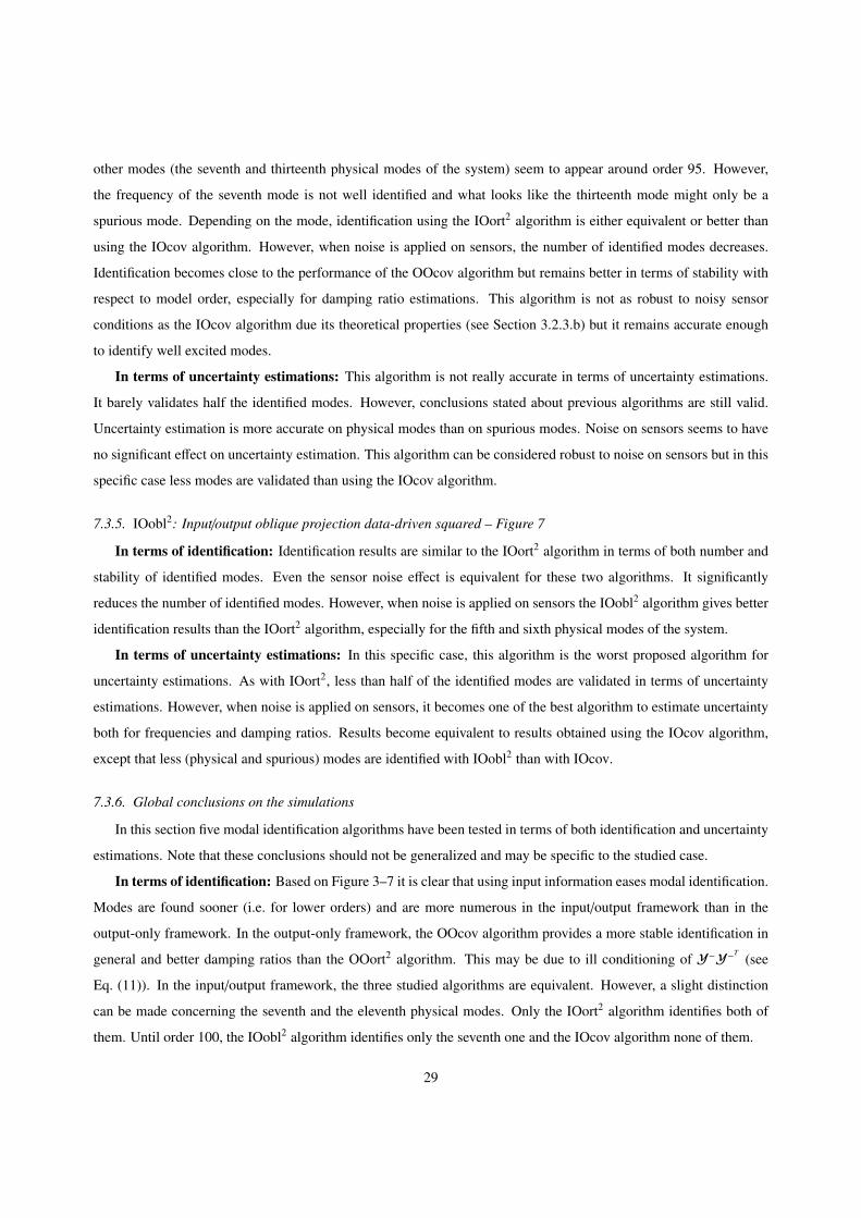
other modes (the seventh and thirteenth physical modes of the system) seem to appear around order 95. However,

the frequency of the seventh mode is not well identified and what looks like the thirteenth mode might only be a

spurious mode. Depending on the mode, identification using the IOort2 algorithm is either equivalent or better than

using the IOcov algorithm. However, when noise is applied on sensors, the number of identified modes decreases.

Identification becomes close to the performance of the OOcov algorithm but remains better in terms of stability with

respect to model order, especially for damping ratio estimations. This algorithm is not as robust to noisy sensor

conditions as the IOcov algorithm due its theoretical properties (see Section 3.2.3.b) but it remains accurate enough

to identify well excited modes.

In terms of uncertainty estimations: This algorithm is not really accurate in terms of uncertainty estimations.

It barely validates half the identified modes. However, conclusions stated about previous algorithms are still valid.

Uncertainty estimation is more accurate on physical modes than on spurious modes. Noise on sensors seems to have

no significant effect on uncertainty estimation. This algorithm can be considered robust to noise on sensors but in this

specific case less modes are validated than using the IOcov algorithm.

7.3.5. IOobl2: Input/output oblique projection data-driven squared – Figure 7

In terms of identification: Identification results are similar to the IOort2 algorithm in terms of both number and

stability of identified modes. Even the sensor noise effect is equivalent for these two algorithms. It significantly

reduces the number of identified modes. However, when noise is applied on sensors the IOobl2 algorithm gives better

identification results than the IOort2 algorithm, especially for the fifth and sixth physical modes of the system.

In terms of uncertainty estimations: In this specific case, this algorithm is the worst proposed algorithm for

uncertainty estimations. As with IOort2, less than half of the identified modes are validated in terms of uncertainty

estimations. However, when noise is applied on sensors, it becomes one of the best algorithm to estimate uncertainty

both for frequencies and damping ratios. Results become equivalent to results obtained using the IOcov algorithm,

except that less (physical and spurious) modes are identified with IOobl2 than with IOcov.

7.3.6. Global conclusions on the simulations

In this section five modal identification algorithms have been tested in terms of both identification and uncertainty

estimations. Note that these conclusions should not be generalized and may be specific to the studied case.

In terms of identification: Based on Figure 3–7 it is clear that using input information eases modal identification.

Modes are found sooner (i.e. for lower orders) and are more numerous in the input/output framework than in the

output-only framework. In the output-only framework, the OOcov algorithm provides a more stable identification in

general and better damping ratios than the OOort2 algorithm. This may be due to ill conditioning of Y−Y−T

(see

Eq. (11)). In the input/output framework, the three studied algorithms are equivalent. However, a slight distinction

can be made concerning the seventh and the eleventh physical modes. Only the IOort2 algorithm identifies both of

them. Until order 100, the IOobl2 algorithm identifies only the seventh one and the IOcov algorithm none of them.

29

0.3 0.4 0.5 0.6 0.7 0.8 0.9 1

10

20

30

40

50

60

70

80

90

100Case 1 − Algorithm OIsqobl : Frequencies

Mod

el o

rder


mod

elor

der


0.3 0.4 0.5 0.6 0.7 0.8 0.9 1

10

20

30

40

50

60

70

80

90

100Case 2 − Algorithm OIsqobl : Frequencies

Mod

el o

rder

Normalized natural frequencynormalized frequencym

odel

orde

r(b) Normalized frequencies – with noise on sensors

0 10 20 30 40 50 60 70 80 90 100

10

20

30

40

50

60

70

80

90

100Case 1 − Algorithm OIsqobl : Damping

Mod

el o

rder

./..damping ratio

mod

elor

der


0 10 20 30 40 50 60 70 80 90 100

10

20

30

40

50

60

70

80

90

100Case 2 − Algorithm OIsqobl : Damping

Mod

el o

rder

./..damping ratio

mod

elor

der


Figure 7: IOobl2 – Monte Carlo stabilization charts with success test values for orders 1 to 100

Concerning noise on sensors effect, it was shown that it strongly depends on the algorithm. Remind that the

presented results are an average of stable mode estimates for different identifications. Based on that, noise has no

effect on the IOcov algorithm and almost no effect on the OOcov algorithm. It reduces the number of modes and

improves their stability when using OOort2, IOort2 and IOobl2.

In terms of uncertainty estimations: Concerning the use of input information, it seems to have no clear effect on

uncertainty estimations. Validations are not better in the input/output framework than in the output-only framework.

Both the OOort2 and IOcov algorithms provide much more validated uncertainty estimations than OOcov, IOort2

and IOobl2. The OOcov algorithm is the only studied algorithm which is not robust to noise on sensors. Noise

has absolutely no influence on uncertainty estimated by the IOcov algorithm. It has no clear impact when using

30

0.5 0.55 0.6 0.65 0.7 0.75 0.8 0.85 0.9 0.95 1

5

10

15

20

25

30

35

40

45

50

55

60

Mod

el o

rder

Normalized natural frequency

ossss

o sf ss ss sf sf ss sf sf o ss f ss f s os s s ss s s ss s sos f o s os s f s fs s s s ss f d s os s s s ss s f s ss s s s ss s s s fs f s s ss s s s ss ff f s ss sf s s ss o s s s ss s s s s ss d s f o s ss o f s o s ss s s s s s ss s s s f s ss s s s s s sf f s s s s ss s s f f s ss f s s s s ss s s s s s sf f s s f s ss s s s f s ss s s s f s ss s s s f s ss s s s s s ss s s s s s ss s s s s s ss s s s s s ss s s s s s ss s s s f s ss s so s s s ss s sf s s s ss s ss s s s s

Case 1 − Algorithm OOcov : Frequencies

normalized frequency

mod

elor

der

0.5 0.55 0.6 0.65 0.7 0.75 0.8 0.85 0.9 0.95 1

5

10

15

20

25

30

35

40

45

50

55

60

Mod

el o

rder


ossss

o sf ss ss sf sf ss sf sf o ss f ss f ss s ss s ss s ss f ss s o ss s ss f o s os s s s ss s f s ss s s s ss s s s fs f s s ss s s s ss f f s ss s s s ss s s s ss ss o o s os o f s o s ss s s s s s ss s s s f s ss s s s s s sf f s s s s ss s s f f s ss f s s s s ss s s s s s sf f s s f s ss s s s f s ss s s s f s ss s s s f s ss s s s s s ss s s s s s ss s s s s s ss s s s s s ss s s s s s ss s s s f s ss s s s s ss o so s s s ss s ss s s s s

Case 1 − Algorithm OOcov : Frequencies

normalized frequencym

odel

orde

r

Figure 8: OOcov: Output-only covariance-driven – stabilization charts of normalized frequencies (left: full, right: cleaned)

either OOort2 or IOort2. Finally, noise on sensors makes IOobl2 the best proposed algorithm in terms of uncertainty

estimations.

8. Application to real data from in-flight vibration tests

After validation on Ns = 200 simulations, the five considered algorithms are used to compute identifications with

uncertainty estimations based on real measured data. These data have been obtained during in-flight vibration tests of

an unnamed aircraft. Known excitations are symmetric white noises performed by both left and right control surfaces

of the aircraft during T = 180 s and sampled at rate Fs = 250 Hz. Responses are obtained by No = 50 sensors along

the aircraft under both the known excitation and in addition unknown external environmental excitations. To estimate

auto- and cross-covariances (see Appendix A), the N = 44,828 time samples of each input and output are divided

into 10 blocks. Estimation results are presented within classical stabilization diagrams added by confidence intervals

( f ±σ f ). Only frequencies are presented. Modes are normalized by the highest displayed frequency value. Estimates

are then plotted from 0 to 1 for the frequency range and for orders from 1 to 60.

It is empirically observed that spurious modes often have higher uncertainty values than physical ones. Confidence

intervals can then be used to clean up stabilization charts by applying a threshold based on uncertainty values. In the

figures, the original uncleaned stabilization diagrams are shown on the left, whereas the cleaned stabilization diagrams

using the uncertainty-based threshold are shown. Thresholds on uncertainties have been set to 0.25 Hz for frequencies

and 100 h for damping ratios. Results are as follows:

• OOcov, Figure 8: Seven modes are clearly identified. An eighth one appears at order 58. There are few spurious

modes. Uncertainty-based clean up is relevant. It removes only spurious or unstable modes. One can observe that

more stable modes have a smaller uncertainty estimation. Moreover, uncertainties are coherent with operationally

31

0.5 0.55 0.6 0.65 0.7 0.75 0.8 0.85 0.9 0.95 1

5

10

15

20

25

30

35

40

45

50

55

60

Mod

el o

rder


dosss

o sf ss ss ss ss sf fs fs ss o ss o fs f ss s ss s ss s fos s d s os s o s os f o s fs s o s os s f s sf f s s ss s s s ss s s s ss f f s ff o o f s ss s s s s ss f f f s ss o f s f f ff f s f s o ss s s f fo fs s s f o f ff f s s o s s os s s s s s s ss s s s s f s ds s s s s f sds s s s s s sfs s s s s s sss s s s s s sss s s s s s sss s s s s s sds s s s s s sss s s s s s ssf f f s f o f ss s s s f f s ss s s s s s s ss f so s s d s ss s sf s s f s s

ss s f s s f f sss f o s s s s s

s s ss s s s f sCase 1 − Algorithm OOsqort : Frequencies


mod

elor

der

0.5 0.55 0.6 0.65 0.7 0.75 0.8 0.85 0.9 0.95 1

5

10

15

20

25

30

35

40

45

50

55

60

Mod

el o

rder


osss

o sf ss ss ss ss sf fs fs ss o ss o fs f ss s ss s ss s fs s ss s ss f o s os s s os s o s sf f s s ss s s s ss s s s ss f f s ff o f s ss s s ss o f s ss f s ff o s f ss s s f fs s s f f of f s s o s ss s s s s s ss s s s s f ss s s s s f ss s s s s s ss s s s s s ss s s s s s ss s s s s s ss s s s s s ss s s s s s ss s s s s s sf f f s f f ss s s s f s ss s s s s s ss f s s s s ss s s s s s

ss s s s o o sss f o s s s s s

s s ss s s s f sCase 1 − Algorithm OOsqort : Frequencies


odel

orde

r

Figure 9: OOort2: Output-only orthogonal projection data-driven squared – stabilization charts of normalized frequencies (left: full, right: cleaned)

0.5 0.55 0.6 0.65 0.7 0.75 0.8 0.85 0.9 0.95 1

5

10

15

20

25

30

35

40

45

50

55

60

Mod

el o

rder


oo

fssssd

s sss

s sss

s ssossfssfs

ss ss oss

s s s os s s s

s ssss oosss sosss sssss sfsss ssss

ssfssssffos

s o s s s ss f s s s s

sssssss sssss

ssssssssf osss

s sofssss s s f f s ss s s s s s ss s s s f s ss s s s s s ss s s s f s ss s s s s s ss s s s s s ss s s s s s ss s s s s s ss s s s s s s

ss s s s s ss s s s f s ss f so s f s ss s sf s s s ss s ss s f s ss s sf s s s ss s ss s s s ss s ss s s s ss s ss s s s ss s ss s s s ss s ss s s s ss s sf s s s ss s ss s s s ss s ss s s s s

Case 1 − Algorithm OIcov : Frequencies


mod

elor

der

0.5 0.55 0.6 0.65 0.7 0.75 0.8 0.85 0.9 0.95 1

5

10

15

20

25

30

35

40

45

50

55

60

Mod

el o

rder


oo

fssssd

s sss

s sss

s ssossfssfs

ss ssss

s s ss s s

ssss osss sosss sssss sfsss ssss

ssfssssffs

s o s s s ss f s s s s

sssssss sssss

ssssssssfsss

s sofssss s s f f s ss s s s s s ss s s s f s ss s s s s s ss s s s f s ss s s s s s ss s s s s s ss s s s s s ss s s s s s ss s s s s s s

ss s s s s ss s s s f s ss f so s f s ss s sf s s s ss s ss s f s ss s sf s s s ss s ss s s s ss s ss s s s ss s ss s s s ss s ss s s s ss s ss s s s ss s sf s s s ss s ss s s s ss s ss s s s s

Case 1 − Algorithm OIcov : Frequencies


mod

elor

der

Figure 10: IOcov: Input/output covariance-driven – stabilization charts of normalized frequencies (left: full, right: cleaned)

observed deviations.

•OOort2, Figure 9: As with the OOcov algorithm, seven modes are clearly identified. However, they are much less

stable with respect to model order. Moreover, this identification contains more spurious modes than the identification

obtained with OOcov. This example shows how useful the uncertainty-based clean up may be.

• IOcov, Figure 10: It is the first presented algorithm using input information. On can observe that modes appear

“sooner” (i.e. for lower orders) when input information is used. Here, modes are also more stable and have smaller

uncertainty values. Only a few spurious modes are identified (only 7 points in the whole stabilization charts). Once

again, as with previous algorithms, one can observe that uncertainty estimates are smaller for more stable modes.

• IOort2, Figure 11: This algorithm gives the worst identification and higher uncertainty values. However it clearly

32

0.5 0.55 0.6 0.65 0.7 0.75 0.8 0.85 0.9 0.95 1

5

10

15

20

25

30

35

40

45

50

55

60

Mod

el o

rder


oo

fsss

o sssss

s sf ss sf s

sss o ss o ss s ss s ss s ss s ss f s os s s os s s ss s s ss s s fs s s os s s ss s s ss s o s os f o s fs s o s fs f f s fs f f s ss s s s fs s s s sf o f f s s

ss f s s fss s f s f

s s s s s fs s s f o s fs f s s s s fs f s s f s fs s s f o s fs s s f s s s

ss s s s s fs s s s s s fs s s s s s ss f s s s s fs s s s s s fs s s s d s fs s s s f s ss s s s s s fs f s s s s f

o s s s s s f ff s f s s f s f

ss so s f s fs s s s s s f

Case 1 − Algorithm OIsqort : Frequencies


mod

elor

der

0.5 0.55 0.6 0.65 0.7 0.75 0.8 0.85 0.9 0.95 1

5

10

15

20

25

30

35

40

45

50

55

60

Mod

el o

rder


oo

fsss

o sssss

s sf ss sf s

sss ss o ss s ss s ss s ss s ss f ss s ss s ss s ss s ss s s os s ss s ss s s os f o s fs s o s fs f f s fs f f s ss s s s fs s s s sf o f f s s

ss f s s fss s f s f

s s s s s fs s s f s fs f s s s fs f s s s fs s s f o s fs s s f s s s

ss s s s fs s s s o s fs s s s ss o s s o s fs s s s s s fs s s s d s fs s s s f ss s s s s s os f s s s s fs s s s s f fs f s s f s f

ss s s f s fs s s s s s

Case 1 − Algorithm OIsqort : Frequencies


odel

orde

r

Figure 11: IOort2: Input/output orthogonal projection data-driven squared – stabilization charts of normalized frequencies (left: full, right: cleaned)

shows as well that the more stable a mode, the smaller its uncertainty estimation.

0.5 0.55 0.6 0.65 0.7 0.75 0.8 0.85 0.9 0.95 1

5

10

15

20

25

30

35

40

45

50

55

60

Mod

el o

rder


oosfs

o so ff ss sf sf ss sf sf o ss f ss f ss s ss s sos s f ss s sss s f ss s o s os s s s ss s f s fs f s s ss s s s ss s s s ss o f f s ss f f s s ss f f f s ss s s s s ss s s f s fs f s s sf fs s s s o s fs f s f o s fs f s f f s ss s s s s s ss s s s s s ss f s f f s ss s s s s s ss s s s s s ss s s s s s ss s s s s s ss s s s s s ss s s s s s ss s s s s s ss s s s s s ss f so s s s ss s ss s s s s

ss s f s s s sss s s s s s sss s s s s s s

s s sf s s s ss f ss s s s ss s ss s s s ss s ss s s s s

Case 1 − Algorithm OIsqobl : Frequencies


mod

elor

der

0.5 0.55 0.6 0.65 0.7 0.75 0.8 0.85 0.9 0.95 1

5

10

15

20

25

30

35

40

45

50

55

60

Mod

el o

rder


osfs

o so ff ss sf sf ss sf sf o ss f ss f ss s ss s ss s ss s ss s ss s o s os s s s ss s f s fs f s s ss s s s ss s s s ss o f f s ss f f s s ss f f s ss o s s s ss s s f s fs f s s ss s s s s os f s f o s fs f s f f s ss s s s s s ss s s s s s ss f s f f s ss s s s s s ss s s s s s ss s s s s s ss s s s s s ss s s s s s ss s s s s s ss s s s s s ss s s s s s ss f s s s s ss s s s s s s

ss s o s s s sss s s s s s sss s s s s s s

s s sf s s s ss f ss s s s ss s ss s s s ss s ss s s s s

Case 1 − Algorithm OIsqobl : Frequencies


mod

elor

der

Figure 12: IOobl2: Input/output oblique projection data-driven squared – stabilization charts of normalized frequencies (left: full, right: cleaned)

• IOobl2, Figure 12: Identification is similar to the IOcov algorithm. In this specific case, these two algorithms

provide the best identification and small uncertainty values.

9. Discussion

In this paper, variance estimates were developed for output-only and input/output system identification schemes

generalizing [27, 28] previously developed for the OOcov (output-only covariance-driven) subspace algorithm. Based

on this method, variance expressions have been developed for OOort2 (output-only orthogonal projection data-driven

33

squared), IOcov (input/output covariance-driven), IOort2 (input/output orthogonal projection data-driven squared) and

IOobl2 (input/output oblique projection data-driven squared) algorithms. Providing also a computation scheme for the

mode shapes, the paper focusses on the estimation of the modal frequencies and damping ratios, which are parameters

of interest for operational modal analysis during in flight tests.

These five modal identification algorithms have been validated in terms of both identification and variance estima-

tions. In this validation, their robustness to sensor noise has also been tested. Finally they have been applied on real

measurements. Besides an academic test case on a mass-spring chain, simulations and real data were provided on an

unnamed aircraft from industrial cases and results have been normalized to allow publication.

The validation of the modal identification algorithms and their variance computation were based on Monte Carlo

simulations. Output-only and input/output algorithms have been compared. In the investigated examples, the number

of identified modes increases and modes appear at lower orders when using input information. Furthermore, the

variance decreases with input information when using the appropriate algorithms. The validation of the variance

computation was equally comparable with or without using inputs. In the academic test case, the results of the variance

computation were close to the respective variances from the Monte Carlo simulations for all algorithms, including the

use of sensor noise. In the industrial test cases, the effect of sensor noise has been shown strongly dependent on the

respective algorithms. For the OOcov algorithm a degradation of both identification and variance estimations could

be observed with sensor noise. For the OOort2 algorithm, it was a slight improvement of both identification in terms

of stability with respect to model order and variance estimations. Sensor noise did not change validation results for

the IOcov algorithm. In terms of identification, impact of noise was similar with IOort2 and IOobl2 algorithms. One

could observe a reduction of the number of identified modes. Only the more stable ones were found again with sensor

noise. However, in terms of uncertainty validation, a huge improvement was observed for the IOobl2 algorithm.

After validation, the considered algorithms have been tested on real-life measured data obtained during in-flight

vibration tests. It appeared that non-physical poles (i.e., spurious modes) have often much higher variance values than

physical ones (real modes of the structure). This allows to use variance estimation to clean up stabilization charts and

then to ease their interpretation during identification. Furthermore, the mode selection from the stabilization diagram

could be supported by the actual computed uncertainty bounds. While different model orders indeed help to reliably

identify the modes, the results show that the model order should not be too high in same cases. There, the results

deteriorate slightly or the uncertainty estimation is less validated for high orders, which might be due to overfitting or

worse conditioning of the involved matrices for (pseudo-)inverting in the subspace methods at high orders.

Concerning the efficiency of the algorithms, it seems that input information eases identification and reduces un-

certainty values. However, if only outputs are available, output-only algorithms give relevant results. If the five

algorithms had to be classified in terms of both identification and uncertainty estimations, their ranking could be as

follows:

IOcov > IOobl2 > OOcov > IOort2 > OOort2

34

This classification has to be taken carefully. It cannot be generalized and it could be specific to the test case.

Recall that the chosen approach for variance computation cannot be used directly on data-driven algorithms. In-

deed, the column dimension of data-driven matrices for subspace identification increases with the number of samples.

Hence, they are not compatible with a sample covariance formulation and the perturbation-based approach from [26–

28] cannot be applied directly. Fortunately, as shown in the current paper, the singular value decomposition properties

ensure that the proposed variance computation scheme for the squared subspace algorithms provides equivalent uncer-

tainty bounds for the pair (A,C) obtained from the data-driven algorithms. Thus, frequency, damping ratio and mode

shape estimates are exactly the same using either data-driven algorithms or their squared counterpart. This allows to

use the proposed scheme on the squared subspace matrices to estimate variances of modal parameters from data-driven

algorithms. Still, the actual implementation of the data-driven algorithms may differ from the direct computation of

the subspace matrices and implies usually computation procedures such as QR decomposition [2], which is a supple-

mentary numerical step before the SVD to obtain the observability matrix. While such a step does not change the

variance expressions thanks to the equivalence of the algorithms, it should be incorporated as in [41]. Furthermore,

the efficient numerical framework for the variance computation of [28] should be applied to the new methods from

this paper. With this framework, computation times for all the methods are less than a minute for a whole stabilization

diagram containing model orders until 100 on a standard desktop computer and hardly differ between the different

subspace methods.

Finally, we recall that the input/output methods in this paper have been derived under the premise that the known

inputs are the realization of a stochastic process. The Monte Carlo simulations have shown that this assumption gives

coherent variance estimates with the methods of this paper. The stochastic properties of the inputs contribute to the

variance estimates of the modal parameters. They do not necessarily mean an increase of the variance estimates of the

modal parameters. Taking them into account is necessary for a correct variance estimation. In particular, it has been

demonstrated in Section 6.2 that the variance is correctly estimated at zero in the case of no unknown inputs and no

sensor noise when taking the stochastic properties of the inputs into account. Neglecting the stochastic properties of

the inputs has led to a variance estimate different from zero in this case.

Deterministic inputs are not considered in this paper. Under a few assumptions for the known inputs such as

persistent excitation [2], quasi-stationarity for deterministic signals such as in [21], and under the assumption of both

known deterministic input and unknown stochastic noise, the current approach would be applicable provided the

uncertainty is derived with respect to the noise only, and as long as auto- and cross-covariances can be defined for the

known input as in [9]. The corresponding variance computation could be handled by the current approach as a special

case, where the variance with respect to the functions of the deterministic and known inputs is taken as zero.

35

10. Conclusion

Modal identification is commonly used in industry in the design process for a structure. The uncertainty infor-

mation related to the identified modal parameters is at least as valuable as the modal parameters themselves in order

to judge their quality and confidence. Moreover, in some highly dangerous and expensive vibration tests (e.g. flutter

tests [43]), uncertainty estimations may be very helpful in terms of both safety and cost reduction. In this paper,

the main results are new expressions for variance estimation for four output-only and input/output subspace-based

modal identification algorithms. It has been shown that considering the stochastic properties of the known input leads

to a correct formulation of the variance estimation scheme. Concerning the considered subspace algorithms, it has

been shown how data-driven algorithms as found in [2, 32] can be related to an equivalent covariance-driven form

yielding identical estimates for the pair (A,C). From this remark, covariance estimates for (A,C) and subsequently

for frequencies, damping ratios and mode shapes were derived. The validation of this approach has been carried out

with Monte Carlo simulations, and it has been applied on real in-flight aircraft data. Further work should include the

variance estimation for the pair (B,D) as well as for the modal mass.

Appendix A. Computation of auto- and cross-covariance functions

Let F be the discrete Fourier transform operator, and let a and b be placeholders for two discrete-time signals

(e.g. u and y, or y and y) whose cross-covariance shall be computed. The signals are divided into nb segments a(k) and

b(k), k = 1, . . . , nb, of equal size (with or without overlap). An apodization window is often applied to these segments

to reduce the leakage effect. Fourier transformations of a(k) and b(k) are given by a(k)F

= F [a(k)] and b(k)F

= F [b(k)].

PSD functions of each segment k between a(k)F

and b(k)F

are then S [a(k),b(k)] = a(k)F

(b(k)F

)∗, where ∗ denotes the conjugate

transpose, and PSD functions of a and b are estimated by averaging as S [a,b]def= 1

nb

∑nbk=1 S [a(k),b(k)]. Finally, cross-

covariance functions are obtained by an inverse Fourier transformation as R[a,b] = F −1[S [a,b]]. An advantage of this

approach for computing cross-covariance functions is the possibility to reduce the frequency band by applying a

rectangular window on the estimation of the power spectral density functions. Note that, due to the linearity of F ,

one can also first apply the Fourier transform to the nb PSD functions and then average these nb cross-covariance

functions to obtain the estimation R[a,b]. Also, an important remark concerns the stochastic properties of S [a,b]. If

a(k) and b(k) are ergodic random processes, a(k)F

and b(k)F

are also ergodic random processes by linearity of the Fourier

transformation. The nb PSD functions S [a(k),b(k)] are nb independent and identically distributed (i.i.d.) ergodic random

processes having the same expectation E[S [a(k),b(k)]] = S [a,b] and same covariance ΣS [a(k) ,b(k) ]= ΣS [a′ ,b′] . Their mean S [a,b]

is an estimate of S [a,b] and, by the CLT, follows a normal distribution with expectation E[S [a,b]] = S [a,b] and covariance

ΣS [a,b]= 1

nbΣS [a′ ,b′ ] .

36

Appendix B. From covariance ofH to the modal parameters

Let H be the subspace matrix corresponding to a chosen subspace algorithm, which is given together with an

estimate of Cov(vec(H)). This covariance is propagated to the observability matrix Γp, then to the system matrices

A and C and finally to the modal parameters, as outlined as follows. Matrix Γp is obtained from an SVD of H in

Eq. (15) as Γp = U1S 1/21 . The sensitivity of Γp is obtained by perturbation as ∆Γp = ∆U1S 1/2

1 + U1∆S 1/21 and finally,

using JΓ,H as detailed in [27, 28],

Cov(vec(Γp)) = E[vec(∆Γp)vec(∆Γp)T

]= JΓ,HCov(vec(H))JT

Γ,H

Then, A and C are obtained from Γp, and perturbations on A an C are obtained by perturbations of the equations in

Section 3.3. Then vec(∆A) = JA,Γvec(∆Γp) and vec(∆C) = JC,Γvec(∆Γp). The covariances of A and C write as

ΣA,C = Cov

vec(A)

vec(C)

=

JA,Γ

JC,Γ

JΓ,HΣHJTΓ,H

[JT

A,Γ JTC,Γ

]where JA,Γ and JC,Γ are detailed in [27, 28]. Covariances of modal parameters are finally as in [27, 28].

Appendix C. Proof of Lemma 6

Deriving the product RaR†

bRc, it follows ∆(RaR†

bRc) = ∆RaR†

bRc +Ra∆(R†b)Rc +RaR†

b∆Rc, and it remains to show

the identity

Ra∆(R†b)Rc = −RaR†

b∆(Rb)R†bRc (C.1)

to conclude the proof. Let the SVD of B be given,

B =

[U1 U2

] S 1 0

0 0

VT

1

VT2

= U1S 1VT1 ,

where S 1 contains all non-zero singular values, and UT1 U1 = I. From the SVD of B it follows the SVD of Rb =

BBT = U1S 21UT

1 and its pseudo-inverse R†b = U1S −21 UT

1 . Both sides of (C.1) are now developed. It holds

Ra∆(R†b)Rc = ABT ∆(BBT )†BCT

= AV1S 1UT1 ∆(U1S −2

1 UT1 )U1S 1VT

1 CT

= AV1S 1UT1

(∆U1S −2

1 UT1 + U1∆S −2

1 UT1 + U1S −2

1 ∆UT1

)U1S 1VT

1 CT

= AV1S 1

(UT

1 ∆U1S −21 − S −2

1 ∆S 21S −2

1 + S −21 ∆UT

1 U1

)S 1VT

1 CT (C.2)

and

−RaR†

b∆(Rb)R†bRc = −A(U1S 1VT1 )T (U1S −2

1 UT1 )∆(U1S 2

1UT1 )(U1S −2

1 UT1 )(U1S 1VT

1 CT )

= AV1S 1S −21 UT

1

(−∆U1S 2

1UT1 − U1∆S 2

1UT1 − U1S 2

1∆UT1

)U1S −2

1 S 1VT1 C

T

= AV1S 1

(−S −2

1 UT1 ∆U1 − S −2

1 ∆S 21S −2

1 − ∆UT1 U1S −2

1

)S 1VT

1 CT . (C.3)

37

Since UT1 U1 = I, it follows ∆UT

1 U1 = −UT1 ∆U1 and hence (C.2) and (C.3) are equivalent. Thus, (C.1) holds, proving

the assertion.

Appendix D. Sensitivity of IOobl2: Input/output orthogonal projection data-driven squared

To derive vec(∆HIOobl2 ) in Eq. (21) withHIOobl2 = Ω1Ω†

2R11Ω†

2ΩT1 and

Ω1 =(Y+/U+⊥

) (W−/U+⊥

)T, Ω2 =

(W−/U+⊥

) (W−/U+⊥

)T, and R11 =W−W−T ,

we first show

∆(Ω1Ω†

2R11) = ∆(Ω1)Ω†2R11 −Ω1Ω†

2∆(Ω2)Ω†2R11 + Ω1Ω†

2∆(R11). (D.1)

First, consider the “noisy” case with the presence of non-zero unmeasured inputs (process noise) u and sensor

noise v. For this case, it has been shown in [44] that the term(W−/U+⊥

)is of full row rank. Hence, Ω2 is invertible

and Eq. (D.1) holds since Ω†

2 = Ω−12 and due to the property ∆(Ω−1

2 ) = −Ω−12 ∆(Ω2)Ω−1

2 .

Second, consider the “no noise” case with no unmeasured inputs and no sensor noise. For this case, it has been

shown in [2, Appendix A.1] that the term(W−/U+⊥

)is indeed rank deficient, but that

(W−/U+⊥

)andW− have the

same column space. Due to this property, Lemma 6 can be applied to show Eq. (D.1).

Hence, Eq. (D.1) holds for both the “noisy” and “no noise” cases. Then, a subsequent relationship for ∆HIOobl2 =

∆(Ω1Ω†

2R11Ω†

2ΩT1 ) is straightforward to show, and the relationship for vec(∆HIOobl2 ) in Eq. (21) follows after vector-

ization and re-ordering, where J(1)H ,R

= JH ,Ω1

J(2)H ,R

= JH ,Ω1J(1)Ω1,R

J(3)H ,R

= JH ,Ω1J(2)Ω1,R

+JH ,Ω2J(2)Ω2,R

J(4)H ,R

= JH ,Ω1J(3)Ω1,R

+JH ,Ω2J(1)Ω2,R

J(5)H ,R

= JH ,Ω2 +JH ,R11

JH ,Ω1 = Ω1Ω

†

2R11Ω†

2 ⊗ IpNo + (IpNo ⊗Ω1Ω†

2R11Ω†

2)PpNo,q(No+Ni)

JH ,Ω2 = −Ω1Ω†

2R11Ω†

2 ⊗Ω1Ω†

2 −Ω1Ω†

2 ⊗Ω1Ω†

2R11Ω†

2

JH ,R11 = Ω1Ω†

2 ⊗Ω1Ω†

2J

(1)Ω1,R

= −R10R†

8 ⊗ IpNo

J(2)Ω1,R

= R10R†

8 ⊗ R4R†

8

J(3)Ω1,R

= −(Iq(No+Ni) ⊗ R4R†

8)Pq(No+Ni),pNi

J(1)Ω2,R

= −R10R†

8 ⊗ Iq(No+Ni) − (Iq(No+Ni) ⊗ R10R†

8)Pq(No+Ni),pNi

J(2)Ω2,R

= R10R†

8 ⊗ R10R†

8

References

[1] W. Heylen, S. Lammens, P. Sas, Modal Analysis Theory and Testing, Katholieke Universiteit Leuven, Belgium, 1998.

[2] P. Van Overschee, B. De Moor, Subspace Identification for Linear Systems: Theory, Implementation, Applications, Kluwer, 1996.

[3] E. Reynders, System identification methods for (operational) modal analysis: review and comparison, Archives of Computational Methods

in Engineering 19 (1) (2012) 51–124.

[4] M. Viberg, Subspace-based methods for the identification of linear time-invariant systems, Automatica 31 (12) (1995) 1835–1851.

38

[5] N. Mastronardi, D. Kressner, V. Sima, P. V. Dooren, S. V. Huffel, A fast algorithm for subspace state-space system identification via exploita-

tion of the displacement structure, Journal of Computational and Applied Mathematics 132 (1) (2001) 71–81.

[6] E. Gandino, S. Marchesiello, Identification of a duffing oscillator under different types of excitation, Mathematical Problems in Engineering

2010.

[7] M. Dohler, L. Mevel, Fast multi-order computation of system matrices in subspace-based system identification, Control Engineering Practice

20 (9) (2012) 882–894.

[8] A. Benveniste, L. Mevel, Nonstationary consistency of subspace methods, IEEE Transactions on Automatic Control 52 (6) (2007) 974–984.

[9] L. Ljung, System identification, Wiley Online Library, 1999.

[10] M. Jansson, B. Wahlberg, A linear regression approach to state-space subspace system identification, Signal Processing 52 (2) (1996) 103–

129.

[11] C. T. Chou, M. Verhaegen, Subspace algorithms for the identification of multivariable dynamic errors-in-variables models, Automatica 33 (10)

(1997) 1857–1869.

[12] T. Gustafsson, Subspace identification using instrumental variable techniques, Automatica 37 (12) (2001) 2005–2010.

[13] E. Gandino, L. Garibaldi, S. Marchesiello, Covariance-driven subspace identification: A complete input–output approach, Journal of Sound

and Vibration 332 (26) (2013) 7000–7017.

[14] B. Peeters, G. De Roeck, Reference-based stochastic subspace identification for output-only modal analysis, Mechanical Systems and Signal

Processing 13 (6) (1999) 855–878.

[15] M. Basseville, L. Mevel, M. Goursat, Statistical model-based damage detection and localization: subspace-based residuals and damage-to-

noise sensitivity ratios, Journal of Sound and Vibration 275 (3) (2004) 769–794.

[16] M. Dohler, L. Mevel, Subspace-based fault detection robust to changes in the noise covariances, Automatica 49 (9) (2013) 2734–2743.

[17] L. Mevel, M. Basseville, A. Benveniste, M. Goursat, Merging sensor data from multiple measurement set-ups for non-stationary subspace-

based modal analysis, Journal of Sound and Vibration 249 (4) (2002) 719–741.

[18] A. Guyader, L. Mevel, Covariance-driven subspace methods: input/output vs. output-only, in: Proceedings of the 21st International Modal

Analysis Conference, Kissimmee, FL, USA, 2003.

[19] L. Mevel, A. Benveniste, M. Basseville, M. Goursat, B. Peeters, H. Van der Auweraer, A. Vecchio, Input/output versus output-only data

processing for structural identificationapplication to in-flight data analysis, Journal of Sound and Vibration 295 (3) (2006) 531–552.

[20] M. Dohler, L. Mevel, Modular subspace-based system identification from multi-setup measurements, IEEE Transactions on Automatic Con-

trol 57 (11) (2012) 2951–2956.

[21] M. Viberg, B. Wahlberg, B. Ottersten, Analysis of state space system identification methods based on instrumental variables and subspace

fitting, Automatica 33 (9) (1997) 1603–1616.

[22] D. Bauer, M. Deistler, W. Scherrer, Consistency and asymptotic normality of some subspace algorithms for systems without observed inputs,

Automatica 35 (7) (1999) 1243–1254.

[23] A. Chiuso, G. Picci, The asymptotic variance of subspace estimates, Journal of Econometrics 118 (1) (2004) 257–291.

[24] D. Bauer, Asymptotic properties of subspace estimators, Automatica 41 (3) (2005) 359–376.

[25] M. Raffy, C. Gontier, Statistical asymptotic error on modal parameters in combined deterministic–stochastic identification algorithm, Me-

chanical Systems and Signal Processing 19 (4) (2005) 714–735.

[26] R. Pintelon, P. Guillaume, J. Schoukens, Uncertainty calculation in (operational) modal analysis, Mechanical Systems and Signal Processing

21 (6) (2007) 2359–2373.

[27] E. Reynders, R. Pintelon, G. De Roeck, Uncertainty bounds on modal parameters obtained from stochastic subspace identification, Mechani-

cal Systems and Signal Processing 22 (4) (2008) 948–969.

[28] M. Dohler, L. Mevel, Efficient multi-order uncertainty computation for stochastic subspace identification, Mechanical Systems and Signal

Processing 38 (2) (2013) 346–366.

[29] M. Dohler, X.-B. Lam, L. Mevel, Uncertainty quantification for modal parameters from stochastic subspace identification on multi-setup

39

measurements, Mechanical Systems and Signal Processing 36 (2) (2013) 562–581.

[30] M. Dohler, F. Hille, L. Mevel, W. Rucker, Structural health monitoring with statistical methods during progressive damage test of S101

Bridge, Engineering Structures 69 (2014) 183–193.

[31] E. Reynders, G. D. Roeck, Reference-based combined deterministic–stochastic subspace identification for experimental and operational

modal analysis, Mechanical Systems and Signal Processing 22 (3) (2008) 617–637.

[32] A. Esna Ashari, L. Mevel, Input-output subspace-based fault detection, in: Proc. 8th IFAC Symposium on fault detection, diagnosis and

safety of technical processes (SAFEPROCESS), Mexico City, Mexico, 2012, pp. 204–209.

[33] M. Verhaegen, Application of a subspace model identification technique to identify lti systems operating in closed-loop, Automatica 29 (4)

(1993) 1027–1040.

[34] P. Van Overschee, B. De Moor, N4SID: Subspace algorithms for the identification of combined deterministic-stochastic systems, Automatica

30 (1) (1994) 75–93.

[35] M. Verhaegen, Identification of the deterministic part of MIMO state space models given in innovations form from input-output data, Auto-

matica 30 (1) (1994) 61–74.

[36] E. Hannan, Multiple time series, Wiley New York, 1970.

[37] G. Golub, C. Van Loan, Matrix computations, 3rd Edition, Johns Hopkins University Press, 1996.

[38] A. Benveniste, J.-J. Fuchs, Single sample modal identification of a nonstationary stochastic process, IEEE Transactions on Automatic Control

AC-30 (1) (1985) 66–74.

[39] G. Casella, R. Berger, Statistical inference, Duxbury Press, 2002.

[40] J. Brewer, Kronecker products and matrix calculus in system theory, IEEE Transactions on Circuits and Systems 25 (9) (1978) 772–781.

[41] M. Dohler, X.-B. Lam, L. Mevel, Multi-order covariance computation for estimates in stochastic subspace identification using QR decompo-

sitions, in: Proc. 19th IFAC World Congress, Cape Town, South Africa, 2014.

[42] W. Gersch, On the achievable accuracy of structural system parameter estimates, Journal of Sound and Vibration 34 (1) (1974) 63–79.

[43] C. R. Pickrel, P. J. White, Flight flutter testing of transport aircraft: in-flight modal analysis, in: Proc. 21st International Modal Analysis

Conference, 2003.

[44] P. Van Overschee, B. De Moor, A unifying theorem for three subspace system identification algorithms, Automatica 31 (12) (1995) 1853–

1864.

40

Variance estimation of modal parameters from …Variance estimation of modal parameters from...

Documents

Transcript of Variance estimation of modal parameters from …Variance estimation of modal parameters from...